Embed Size (px)
Citation preview

The Wealth-Consumption Ratio
The MIT Faculty has made this article openly available. Please share how this access benefits you. Your story matters.
Citation Lustig, H., S. Van Nieuwerburgh, and A. Verdelhan. “The Wealth-Consumption Ratio.” Review of Asset Pricing Studies 3, no. 1 (June1, 2013): 38–94.
As Published http://dx.doi.org/10.1093/rapstu/rat002
Publisher Oxford University Press
Version Author's final manuscript
Citable link http://hdl.handle.net/1721.1/88140
Terms of Use Creative Commons Attribution-Noncommercial-Share Alike
Detailed Terms http://creativecommons.org/licenses/by-nc-sa/4.0/

The Wealth-Consumption Ratio∗
Hanno Lustig
UCLA Anderson and NBER
Stijn Van Nieuwerburgh
NYU Stern, NBER, and CEPR
Adrien Verdelhan
MIT Sloan and NBER
∗Lustig: Department of Finance, UCLA Anderson School of Management, Box 951477, Los Angeles,
CA 90095; [email protected]; Tel: (310) 206-6077; http://www.anderson.ucla.edu/x18962.xml. Van
Nieuwerburgh: Department of Finance, Stern School of Business, New York University, 44W. 4th Street, New
York, NY 10012; [email protected]; Tel: (212) 998-0673; http://www.stern.nyu.edu/~svnieuwe.
Verdelhan: MIT Sloan, [email protected]; http://web.mit.edu/adrienv/www/. The authors would like
to thank Dave Backus, Geert Bekaert, John Campbell, John Cochrane, Ricardo Colacito, Pierre Collin-
Dufresne, Bob Dittmar, Greg Duffee, Darrell Duffie, Robert Goldstein, Lars Peter Hansen, John Heaton,
Dana Kiku, Ralph Koijen, Martin Lettau, Francis Longstaff, Sydney Ludvigson, Thomas Sargent, Kenneth
Singleton, Stanley Zin, and participants of the NYU macro lunch, seminars at Stanford GSB, NYU finance,
BU, the University of Tokyo, LSE, the Bank of England, FGV, MIT Sloan, Purdue, LBS, Baruch, Kellogg,
Chicago GSB, Wharton, and conference participants at the SED in Prague, the CEPR meeting in Gerzensee,
the EFA meeting in Ljubljana, the AFA and AEA meetings in New Orleans, the NBER Asset Pricing meeting
in Cambridge, and the NYU Five Star Conference for comments. This work was supported by the National
Science Foundation [grant number 0550910].
1

Abstract
We derive new estimates of total wealth, the returns on total wealth, and the wealth
effect on consumption. We estimate the prices of aggregate risk from bond yields and
stock returns using a no-arbitrage model. Using these risk prices, we compute total
wealth as the price of a claim to aggregate consumption. We find that U.S. households
have a surprising amount of total wealth, most of it human wealth. This wealth is
much less risky than stock market wealth. Events in long-term bond markets, not
stock markets, drive most total wealth fluctuations. The wealth effect on consumption
is small and varies over time with real interest rates.
JEL codes: E21, G10, G12
2

The total wealth portfolio plays a central role in modern asset pricing theory and macroe-
conomics. Total wealth includes real estate, non-corporate businesses, other financial assets,
durable consumption goods, and human wealth. The objective of this paper is to measure
the amount of total wealth, the amount of human wealth, and the returns on each. The
conventional approach to approximating the return on total wealth is to use the return on
an equity index. Our approach is to measure total wealth as the present discounted value of
a claim to aggregate consumption. The discount factor we use is consistent with observed
stock and bond prices. Our preference-free estimation imposes only the household budget
constraint and no-arbitrage conditions on traded assets. According to our estimates, stock
market wealth is only 1% of total wealth while all non-human wealth only 8%. Moreover,
the returns on the vast majority of total wealth differ markedly from equity returns; they
are much lower on average and have low correlation with equity returns. Thus, our results
challenge the conventional approach.
Our main finding is that households in the United States have a surprising amount of
total wealth, $3.5 million per person in 2011 (in 2005 dollars). Of this, 92% is human wealth,
the discounted value of all future U.S. labor income. Our estimation imputes a value of $1
million to an average career spanning 35 years. The high value of total wealth is reflected in
a high average wealth-consumption ratio of 83, much higher than the average equity price-
dividend ratio of 26. Equivalently, the total wealth portfolio earns a much lower risk premium
of 2.38% per year, compared to an equity risk premium of 6.41%. Total wealth returns are
only half as volatile as equity returns. The lower variability in the wealth-consumption ratio
indicates less predictability in total wealth returns. Unlike stocks, most of the variation in
future expected total wealth returns is variation in future expected risk-free rates, and not
variation in future expected excess returns. The correlation between total wealth returns and
stock returns is only 27%, while the correlation with 5-year government bond returns is 94%.
Thus, the destruction and creation of wealth in the U.S. economy are largely disconnected
from events in the stock market and are related to events in the bond markets instead.
3

Between 1979 and 1981 when real interest rates rose, $318,000 of per capita wealth was
destroyed. Afterwards, as real yields fell, real per capita wealth increased steadily from
$860,000 in 1981 to $3.5 million in 2011. Total U.S. household wealth was hardly affected
by the spectacular declines in the stock market in 1973-1974, 2000-2001, and 2007-2009.
The main message from these results is that equity is quite different from the total wealth
portfolio.
A simple back-of-the-envelope Gordon growth model calculation helps explain the high
wealth-consumption ratio. The discount rate on the consumption claim is 3.51% per year
(a consumption risk premium of 2.38% plus a risk-free rate of 1.49% minus a Jensen term
of 0.37%) and its cash-flow growth rate is 2.31%. The Gordon growth formula delivers the
estimated mean wealth-consumption ratio: 83 = 1/(.0351− .0231).
In addition to the low volatility of aggregate consumption growth innovations, the reason
that total wealth resembles a real bond is that the value of a claim to aggregate risky
consumption is similar to that of a claim whose cash flows grow deterministically at the
average consumption growth rate. The latter occurs because innovations to current and
future consumption growth carry a small market price of risk according to our calculations.
This is not a foregone conclusion because the market prices of risk are estimated to be
consistent with observed stock and bond prices. The finding that current consumption
growth innovations are assigned a small price is not a complete surprise. That is the equity
premium puzzle. But, we also know that traded asset prices predict future consumption
growth. This opens up the possibility that shocks to future consumption demand a high
risk compensation. A key finding of our work is that this channel is not strong enough to
generate a consumption risk premium that resembles anything like the equity risk premium.
Discounting consumption at a low rate of return implies that the present discounted value
of the stream (total wealth) is high, arguably higher than commonly believed.
Our methodology also produces new estimates of the marginal propensity to consume
out of wealth. We find that the U.S. consumer spent only 0.76 cents out of the last dollar
4
of wealth, on average over our sample period. The marginal propensity to consume tracks
interest rates: It peaks in 1981 at 1.4 cents per dollar and bottoms out in 2010 at 0.6 cents
per dollar. The 50% drop in the marginal propensity to consume out of wealth occurred
because the newly created wealth between 1981 and 2010 reflected almost exclusively lower
discount rates rather than higher future consumption growth. We estimate that all variation
in the wealth-consumption ratio is due to variation in discount rates.
A key assumption in the paper is that stock and bond returns span all priced sources of
risk. We verify that our unspanned consumption growth innovations are essentially acyclical
and serially uncorrelated. In addition, we check whether the pricing of consumption inno-
vations that are not spanned by innovations to bond yields or stock returns can overturn
our results. Even if we allow for unspanned priced risk that delivers Sharpe ratios equal to
four times the observed Sharpe ratio on stocks, the consumption risk premium remains 2.5
percentage points below the equity risk premium. In the Online Appendix, we show that our
valuation procedure is appropriate even in an economy with heterogeneous agents who face
uninsurable labor income risk, borrowing constraints, and limited asset market participation.
To derive our wealth estimates, we use a vector auto-regression (VAR) model for the state
variables as in Campbell (1991, 1993, 1996). We combine the estimated state dynamics with
a no-arbitrage model for the stochastic discount factor (SDF). As in Duffie and Kan (1996),
Dai and Singleton (2000), and Ang and Piazzesi (2003), the log SDF is affine in innovations
to the state vector while market prices of aggregate risk are affine in the same state vector.
We estimate the market prices of risk by matching salient features of nominal bond yields,
equity returns and price-dividend ratios, and expected returns on factor-mimicking portfolios,
linear combinations of stock portfolios that have the highest correlations with consumption
and labor income growth. This approach is similar to that in Bekaert, Engstrom, and Xing
(2009), Bekaert, Engstrom, and Grenadier (2010), and Lettau and Wachter (2011), who use
affine models to match features of stocks and bonds. By using precisely-measured stock and
bond price data, our approach avoids using data on housing, durable, and private business
5

wealth from the Flow of Funds. These wealth variables are often measured at book values
and with substantial error.
Our approach also avoids making arbitrary assumptions on the expected rate of return
(discount rate) of human wealth, which is unobserved. In earlier work, Campbell (1993),
Shiller (1995), Jagannathan and Wang (1996), and Lettau and Ludvigson (2001a, 2001b) all
make particular, and very different, assumptions on the expected rate of return on human
wealth. In a precursor paper, Lustig and Van Nieuwerburgh (2008) back out human wealth
returns to match properties of consumption data. Bansal, Kiku, Shaliastovich, and Yaron
(2012) emphasize the role of macro-economic volatility in a related exercise. Using market
prices of risk inferred from traded assets, we obtain a new estimate of expected human wealth
returns that fits none of the previously proposed models. We estimate human wealth to be
92% of total wealth. This estimate is consistent with Mayers (1972), who first pointed out
that human capital forms a major part of the aggregate capital stock in advanced economies,
and with Jorgenson and Fraumeni (1989), who also calculate a 90% human wealth share.
Our result is also consistent with the share of human wealth obtained by Palacios (2011) in
a calibrated version of his dynamic general equilibrium production model.
Our results differ from earlier attempts to measure the wealth-consumption ratio and the
return to total wealth. Lettau and Ludvigson (2001a, 2001b) estimate cay, a measure of
the inverse wealth-consumption ratio. Their wealth-consumption ratio has a correlation of
24% with our series. Alvarez and Jermann (2004) do not allow for time-varying risk premia
and measure total wealth returns as a linear combination of equity portfolio returns. They
estimate a smaller consumption risk premium of 0.2%, and hence a much higher average
wealth-consumption ratio.
Our paper connects to the literature that studies the valuation of an asset for which one
only observes the dividend growth and not the price. The retirement and social security
literature studies related questions when it values claims to future labor income (e.g. De
Jong 2008, Geanakoplos and Zeldes 2010, Novy-Marx and Rauh 2011).
6

Our paper also contributes to the large literature on measuring the propensity to consume
out of wealth. The seminal work of Modigliani (1971) suggests that a one dollar increase
in wealth leads to a five-percent increase in consumption. Similar estimates appear in text-
books, models used by central banks, and in monetary and fiscal policy debates [see Poterba
(2000) for a survey]. A wealth effect of five cents on the dollar implies a wealth-consumption
ratio that is four times lower than our estimates, or equivalently, a consumption risk premium
as high as the equity risk premium. Our first contribution to this literature is to propose
a wealth effect on consumption that is much smaller than previously thought. Second, we
are the first to provide an estimate consistent with the budget constraint and no-arbitrage
restrictions.1 Third, we find that the dynamics of this wealth effect relate to the bond mar-
ket rather than stock market dynamics. This would explain the modest contraction in total
wealth and aggregate consumption in response to the large stock market wealth destruction
of 1973-1974 (e.g. Hall 2001). Our results are consistent with Bernanke and Gertler’s (2001)
suggestion that inflation-targeting central banks should ignore movements in asset values
that do not influence aggregate demand. We find that traded assets amount to a relatively
small share of total wealth. As a result, their price fluctuations do not affect much consumer
spending, the largest component of aggregate demand.
Finally, our work contributes to the consumption-based asset pricing literature. It offers
a new set of moments to evaluate their empirical performance. Too often, such models
are evaluated on their implications for equity returns. But the models’ primitives are the
preferences and the dynamics of aggregate consumption growth. Moments of returns on the
consumption claim are the most primitive asset pricing moments and should be the most
informative for testing these models. In contrast, the dividend growth dynamics of stocks
can be altered without affecting equilibrium allocations or prices of traded assets other than
stocks; modeling them entails more degrees of freedom. This paper carries out a comparison
1Ludvigson and Steindel (1999) and Lettau and Ludvigson (2004) start from the household budget con-straint but do not impose the absence of arbitrage, and assume a constant price-dividend ratio on humanwealth.
7

of two leading endowment economy models: the external habit model of Campbell and
Cochrane (1999) and the long-run risk model of Bansal and Yaron (2004). Our work also
has implications for production-based asset pricing models. As Kaltenbrunner and Lochstoer
(2010) point out, such models usually generate the prediction that the claim to dividends
is less risky than the claim to consumption. Our results indicate that this is counterfactual
and that stocks are special. Modeling realistic dividend dynamics (by introducing labor
income frictions, operational leverage, or financial leverage) is necessary to reconcile the low
consumption risk premium with the high equity risk premium.
The rest of the paper is organized as follows. Section 1 describes our measurement
approach conceptually. Section 2 shows how we estimate the risk price parameters and
Section 3 describes the results from that estimation. Section 4 investigates what features of
the model are responsible for which results and investigates an annual instead of a quarterly
version of our model. Section 5 studies the economic implications of our measurement
exercise for the cost of consumption risk and the propensity to consume out of wealth. It
also shows that our conclusions remain valid when there is priced unspanned consumption
risk. Section 6 compares the properties of the wealth consumption ratio in the long-run risk
and external habit models to the ones we estimate in the data. Finally, Section 7 concludes.
An Online Appendix describes our data, presents proofs, details the robustness checks, and
shows that our valuation approach remains valid in an incomplete markets model.
1 Measuring theWealth-Consumption Ratio in the Data
Section 1.1 describes the framework for estimating the wealth-consumption ratio and the
return on total wealth. Section 1.2 presents two methodologies to compute the wealth-
consumption ratio.
8

1.1 Model
The model consists of a state evolution equation and a stochastic discount factor.
1.1.1 State evolution equation
We assume that the N × 1 vector of state variables follows a Gaussian first-order VAR:
zt = Ψzt−1 + Σ12 εt, (1)
with εt ∼ i.i.d.N (0, I) and Ψ is a N ×N matrix. The vector z is demeaned. The covariance
matrix of the innovations is Σ; the model is homoscedastic. We use a Cholesky decomposition
of the covariance matrix, Σ = Σ12Σ
12′, which has non-zero elements only on and below the
diagonal. We discuss the elements of the state vector in detail below. Among other elements,
the state zt contains real aggregate consumption growth, the nominal short-term interest
rate, and inflation. Denote consumption growth by ∆ct = µc + e′czt, where µc denotes the
unconditional mean consumption growth rate and the N × 1 vector ec is the column of a
N ×N identity matrix that corresponds to the position of ∆c in the state vector. Likewise,
the nominal 1-quarter rate is y$t (1) = y$0(1)+ e′ynzt, where y$0(1) is the unconditional average
and eyn the selector vector. Similarly, πt = π0 + e′πzt is the (log) inflation rate between t− 1
and t. All lowercase letters denote logs. The next section contains details on the estimation
of the VAR and Appendix A describes the data sources and definitions in detail.
1.1.2 Stochastic discount factor
We specify a stochastic discount factor (SDF) familiar from the no-arbitrage term structure
literature, following Ang and Piazzesi (2003). The nominal pricing kernel M$t+1 = exp(m$
t+1)
is conditionally log-normal:
m$t+1 = −y$t (1)−
1
2Λ′
tΛt − Λ′tεt+1. (2)
9

The real pricing kernel is Mt+1 = exp(mt+1) = exp(m$t+1 + πt+1); it is also conditionally
Gaussian.2 The innovations in the vector εt+1 are associated with a N × 1 market price of
risk vector Λt of the affine form:
Λt = Λ0 + Λ1zt,
The N × 1 vector Λ0 collects the average prices of risk while the N ×N matrix Λ1 governs
the time variation in risk premia.
1.2 The wealth-consumption ratio
We explore two methods to measure the wealth-consumption ratio. The first one uses con-
sumption strips and avoids any approximation while the second approach builds on the
Campbell (1991) approximation of log returns.
1.2.1 Consumption strips
A consumption strip of maturity τ pays realized consumption at period τ , and nothing in the
other periods. Under a no-bubble constraint on total wealth, the wealth-consumption ratio
is the sum of the price-dividend ratios on consumption strips of all horizons (Wachter 2005):
Wt
Ct= ewct =
∞∑
τ=0
P ct (τ), (3)
where P ct (τ) denotes the price of a τ period consumption strip divided by the current con-
sumption. Appendix B proves that the log price-dividend ratio on consumption strips are
affine in the state vector and shows how to compute them recursively.
If consumption growth were unpredictable and its innovations carried a zero risk price,
then consumption strips would be priced like real zero-coupon bonds.3 The consumption
2Note that the consumption-CAPM is a special case of this, where mt+1 = log β − αµc − αηt+1 and ηt+1
denotes the innovation to real consumption growth and α the coefficient of relative risk aversion.3First, if aggregate consumption growth is unpredictable, i.e., e′
cΨ = 0, then innovations to future con-
sumption growth are not priced. Second, if prices of current consumption risk are zero, i.e., e′cΣ
1
2Λ1 = 0 and
e′cΣ
1
2Λ0 = 0, then innovations to current consumption are not priced.
10

strips’ dividend-price ratios would equal yields on real bonds (with the coupon adjusted for
growth µc). In this special case, all variation in the wealth-consumption ratio would be
traced back to the real yield curve.
1.2.2 Total wealth returns
Consumption strips allow for an exact definition of the wealth-consumption ratio, but they
call for the estimation of an infinite sum of bond prices. A second approximate method
delivers both a more practical and elegant definition of the wealth-consumption ratio. In
our empirical work, we check that both methods deliver similar results.
In our exponential-Gaussian setting, the log wealth-consumption ratio is an affine func-
tion of the state variables. To show this result, we start from the aggregate budget constraint:
Wt+1 = Rct+1(Wt − Ct). (4)
The beginning-of-period (or cum-dividend) total wealth Wt that is not spent on aggregate
consumption Ct earns a gross return Rct+1 and leads to beginning-of-next-period total wealth
Wt+1. The return on a claim to aggregate consumption, the total wealth return, can be
written as:
Rct+1 =
Wt+1
Wt − Ct=
Ct+1
Ct
WCt+1
WCt − 1.
We use the Campbell (1991) approximation of the log total wealth return rct = log(Rct)
around the long-run average log wealth-consumption ratio Ac0 ≡ E[wt − ct],
4
rct+1 ≃ κc0 +∆ct+1 + wct+1 − κc
1wct. (5)
The linearization constants κc0 and κc
1 are non-linear functions of the unconditional mean
4Throughout, variables with a subscript zero denote unconditional averages.
11

wealth-consumption ratio Ac0:
κc1 =
eAc0
eAc0 − 1
> 1 and κc0 = − log
(eA
c0 − 1
)+
eAc0
eAc0 − 1
Ac0. (6)
Proposition 1. The log wealth-consumption ratio is approximately a linear function of the
(demeaned) state vector zt:
wct ≃ Ac0 + Ac′
1 zt,
where the mean log wealth-consumption ratio Ac0 is a scalar and Ac
1 is the N × 1 vector,
which jointly solve:
0 = κc0 + (1− κc
1)Ac0 + µc − y0(1) +
1
2(ec + Ac
1)′Σ(ec + Ac
1)− (ec + Ac1)
′Σ12
(Λ0 − Σ
12′eπ
)(7)
0 = (ec + eπ + Ac1)
′Ψ− κc1A
c′1 − e′yn − (ec + eπ + Ac
1)′Σ
12Λ1. (8)
The proof in appendix B conjectures an affine function for the log wealth-consumption
ratio, imposes the Euler equation for the log total wealth return, and solves for the coefficients
of the affine function as verification of the conjecture. The resulting expression for wct is an
approximation only because it relies on the log-linear approximation of returns in equation
(5). This log-linearization is the only approximation in our procedure. Once we estimate
the market prices of risk Λ0 and Λ1 below, equations (7) and (8) allow us to solve for the
mean log wealth-consumption ratio (Ac0) and its dependence on the state (Ac
1).5
5Equations (7) and (8) form a system of N +1 non-linear equations in N +1 unknowns. It is a non-linearsystem because of equation (6), but is well-behaved and can easily be solved numerically.
12

1.2.3 Consumption risk premium
Proposition 1 and the total wealth return definition in (5) jointly imply the following log
total wealth return:
rct+1 = rc0 + [(ec + Ac1)
′Ψ− κc1A
c′1 ] zt + (e′c + Ac′
1 )Σ12 εt+1, (9)
rc0 = κc0 + (1− κc
1)Ac0 + µc, (10)
where equation (10) defines the unconditional mean total wealth return rc0. The consumption
risk premium, the expected log return on total wealth in excess of the log real risk-free rate
yt(1) corrected for a Jensen term, follows from the Euler equation Et[Mt+1Rct+1] = 1:
Et
[rc,et+1
]≡ Et
[rct+1 − yt(1)
]+
1
2Vt[r
ct+1] = −Covt
[rct+1, mt+1
](11)
= (ec + Ac1)
′Σ12
(Λ0 − Σ
12′eπ
)+ (ec + Ac
1)′Σ
12Λ1zt.
The first term on the last line is the average consumption risk premium. This is a key object
of interest, which measures how risky total wealth is. The second (mean-zero) term governs
the time variation in the consumption risk premium.
1.2.4 Growth conditions
Given the no-bubble constraint, there is an approximate link between the coefficients in
the affine expression of the wealth-consumption ratio and the coefficients of the strip price-
dividend ratios P ct (τ) = exp(Ac(τ) +Bc(τ)′zt):
exp(Ac0) ≃
∞∑
τ=0
exp(Ac(τ)) and exp(Ac1) ≃
∞∑
τ=0
exp(Bc(τ)). (12)
A necessary condition for this first sum to converge and hence produce a finite average
wealth-consumption ratio is that the consumption strip risk premia are positive and large
13

enough in the limit (as τ → ∞):
(ec +Bc(∞))′ Σ12
(Λ0 − Σ
12 eπ
)> µc − y0(1) +
1
2(ec +Bc(∞))′ Σ (ec +Bc(∞)) .
We refer to this inequality as the growth condition. Because average real consumption growth
µc exceeds the average real short rate y0(1) in the data, the right-hand side of the inequality
is positive. When all the risk prices in Λ0 are zero, this condition is obviously violated. It
implies a lower bound for the consumption risk premium.
1.3 Human wealth
The same way we priced a claim to aggregate consumption, we price a claim to aggregate
labor income. Human wealth is the present value of the latter claim. We impose that the
conditional Euler equation for human wealth returns is satisfied and obtain a log price-
dividend ratio, which is also approximately affine in the state: pdlt = Al0 + Al
1zt. (See
Proposition 2 in Online Appendix B.1.) By the same token, the conditional risk premium
on the labor income claim is affine in the state vector (see equation B.5 in Online Appendix
B.1).
2 Estimating the Market Prices of Risk
In order to recover the dynamics of the wealth-consumption ratio and of the return on wealth,
we need to estimate the market prices of risk Λ0 and Λ1. This section details our estimation
procedure. Section 2.1 describes the state vector. Section 2.2 lists the additional restrictions
we impose on our framework. Section 2.3 describes the estimation technique.
To implement the model, we need to take a stance on what observables describe the
aggregate dynamics of the economy. The de minimis state vector contains the nominal
short rate, realized inflation, and the cash flow growth dynamics of the two cash flows this
paper sets out to price: consumption and labor income. In this section, we lay out our
14
benchmark model, which contains substantially richer state dynamics than contained in
these four variables. The richness stems from a desire to infer the market prices of risk
from a model that accurately prices the bonds of various maturities, the equity market,
and that takes into account some cross-sectional variation across stocks. Section 4 explores
special cases of the benchmark model, with fewer state variables, in order to understand
what elements are crucial for our main findings.
2.1 Benchmark state vector
Our benchmark state vector is:
zt = [CPt, y$t (1), πt, y
$t (20)− y$t (1), pd
mt , r
mt , r
fmpct , rfmpy
t ,∆ct,∆lt]′.
The first four elements represent the bond market variables in the state, the next four
represent the stock market variables, the last two variables represent the cash flows. The
state contains in order of appearance: the Cochrane and Piazzesi (2005) factor (CP ), the
nominal short rate (yield on a 3-month Treasury bill), realized inflation, the spread between
the yield on a 5-year Treasury note and a 3-month Treasury bill, the price-dividend ratio
on the CRSP stock market, the real return on the CRSP stock market, the real return on
a factor-mimicking portfolio for consumption growth, the real return on a factor-mimicking
portfolio for labor income growth, real per capita consumption growth, and real per capita
labor income growth. We recall that lower-case letters denote natural logarithms. This
state vector is observed at quarterly frequency from 1952.I until 2011.IV (240 observations).
In a robustness check, we also consider annual data from 1952 to 2011. The Cholesky
decomposition of the residual covariance matrix, Σ = Σ12Σ
12′, allows us to interpret the shock
to each state variable as the sum of the shocks to all the preceding state variables and an
own shock that is orthogonal to all previous shocks. Consumption and labor income growth
are ordered after the bond and stock variables because we use the prices of risk associated
15
with the first eight innovations to value the consumption and labor income claims.
The goal of our exercise is to price claims to aggregate consumption and labor income
using as much information as possible from traded assets. Thus, the choice of state variables
is motivated by a desire to capture all important dynamics of bond and stock prices. Many of
the state variables have a long tradition in finance as predictors of stock and bond returns.6
2.1.1 Expected consumption growth
Equally important is a rich specification of the cash flows we want to price: consump-
tion and labor income growth. First, our state vector includes variables like interest rates
(Harvey 1988), the price-dividend ratio, and the slope of the yield curve (Ang, Piazzesi, and
Wei 2006) that have been shown to forecast future consumption growth. The predictability
of future consumption growth by stock and bond prices whose own shocks carry non-zero
prices of risk results in a risk premium to future consumption growth innovations and thus
to create a wedge between the risky and the trend consumption claims. Having richly spec-
ified expected consumption growth dynamics alleviates the concern that the model misses
important (priced) shocks to expected consumption growth. Second, the modest correlation
(29%) of the aggregate stock market portfolio with consumption growth motivates us to use
additional information from the cross-section of stocks to learn more about contemporane-
ous shocks to consumption and labor income claims. We use the 25 size- and value-portfolio
returns to form a consumption growth factor-mimicking portfolio (FMP) and a labor income
growth FMP. The consumption (labor income) growth FMP has a 36% (36%) correlation
with actual consumption. Pricing these FMP well alleviates the concern that our model
misses important shocks to current consumption innovations.
Our state variables zt explain 29% of variation in ∆ct+1. The volatility of annualized
expected consumption growth is 0.49%, more than one-third of the volatility of realized
6For example, Ferson and Harvey (1991) study the yield spread, the short rate, and consumption growthas predictors of stocks, while Cochrane and Piazzesi (2005) emphasize the importance of the CP factor topredict bond returns.
16

consumption growth, while the first-order autocorrelation of expected consumption growth
is 0.70 in quarterly data. This shows non-trivial consumption growth predictability, in line
with the literature. Figure 1 plots the (annualized) one-quarter-ahead expected consump-
tion growth series implied by our VAR. The shaded areas are NBER recessions. Expected
consumption growth experiences the largest declines during the Great Recession of 2007.IV-
2009.II, the 1953.II-1954.II recession, the 1957.III-1958.II recession, the 1973.IV-1975.I reces-
sion, the double-dip NBER recession from 1980.I to 1982.IV, and somewhat smaller declines
during the less severe 1960.II-1961.I, 1990.III-1991.I, and 2001.I-2001.IV recessions. Hence,
the innovations to expected consumption growth are highly cyclical. That cyclical risk,
alongside the long-run risk in expected consumption growth implied by the VAR, should
be priced in asset markets. Finally, most of the cyclical variation in consumption growth
is captured by traded asset returns. The correlation of unspanned (orthogonal) consump-
tion growth with the NBER dummy is only -0.01 and not statistically different from zero.
Moreover, these unspanned innovations are essentially uncorrelated over time; the first-order
autocorrelation is -0.05.
Figure 1: Consumption growth predictability
Perce
nt per
year
Expected Consumption Growth
1960 1970 1980 1990 2000 2010−2
−1
0
1
2
3
4
5
The figure plots (annualized) expected consumption growth at quarterly frequency, as implied by the VAR model: Et [∆ct+1] =µc + I′cΨzt, where zt is the N-dimensional state vector.
17

2.2 Restrictions
With ten state variables and time-varying prices of risk, our model has many parameters.
On the one hand, the richness offers the possibility to accurately describe bond and equity
prices without having to resort to latent state variables. On the other hand, there is the risk
of over-fitting the data. To guard against this risk and to obtain stable estimates, we impose
restrictions on our benchmark estimation.
We start by imposing restrictions on the dynamics of the state variable, that is, in the
companion matrix Ψ. Only the bond market variables – first block of four – govern the
dynamics of the nominal term structure; Ψ11 below is a 4 × 4 matrix of non-zero elements.
For example, this structure allows for the CP factor to predict future bond yields, or for
the short-term yield and inflation to move together. It also imposes that stock returns, the
price-dividend ratio on stocks, or the factor-mimicking portfolio returns do not predict future
yields or bond returns; Ψ12 is a 4 × 4 matrix of zeroes. The second block of Ψ describes
the dynamics of the log price-dividend ratio and log return on the aggregate stock market,
which we assume depends on their own lags, as well as the lagged bond market variables.
The elements Ψ21 and Ψ22 are 2×4 and 2×2 matrices of non-zero elements. This allows for
aggregate stock return predictability by the short rate, the yield spread, inflation, the CP
factor, the price-dividend ratio, and its own lag, all of which have been shown in the empirical
asset pricing literature. The FMP returns in the third block have the same predictability
structure as the aggregate stock return, so that Ψ31 and Ψ32 are 2× 4 and 2× 2 matrices of
non-zero elements. In our benchmark model, consumption and labor income growth do not
predict future bond and stock market variables; Ψ14, Ψ24, and Ψ34 are all matrices of zeroes.
Finally, the VAR structure allows for rich cash flow dynamics: expected consumption growth
depends on the first nine state variables and expected labor income growth depends on all
lagged state variables; Ψ41, Ψ42, and Ψ43 are 2 × 4, 2 × 2, and 2 × 2 matrices of non-zero
elements, and Ψ44 is a 2 × 2 matrix with one zero in the upper-right corner. In sum, our
18

benchmark Ψ matrix has the following block-diagonal structure:
Ψ =
Ψ11 0 0 0
Ψ21 Ψ22 0 0
Ψ31 Ψ32 0 0
Ψ41 Ψ42 Ψ43 Ψ44
.
Section 4 also explores various alternative restrictions on Ψ. These do not materially alter
the dynamics of the estimated wealth-consumption ratio. We estimate Ψ by OLS, equation-
by-equation, and we form each innovation as follows zt+1(·) − Ψ(·, :)zt. We compute their
(full rank) covariance matrix Σ.
The zero restrictions on Ψ imply zero restrictions on the corresponding elements of the
market price of risk dynamics in Λ1. For example, the assumption that the stock return and
the price-dividend ratio on the stock market do not predict the bond variables implies that
the market prices of risk for the bond market shocks cannot fluctuate with the stock market
return or the price-dividend ratio. The entries of Λ1 in the first four rows and the fifth and
sixth column must be zero. Likewise, because the last four variables in the VAR do not affect
expected stock and FMP returns, the prices of stock market risk cannot depend on the last
four state variables. Finally, under our assumption that all sources of aggregate uncertainty
are spanned by the innovations to the traded assets (the first eight shocks), the part of the
shocks to consumption growth and labor income growth that is orthogonal to the bond and
stock innovations is not priced. We relax this assumption in section 5.3. Thus, Λ1,41, Λ1,42,
Λ1,43, and Λ1,44 are zero matrices. This leads to the following structure for Λ1:
Λ1 =
Λ1,11 0 0 0
Λ1,21 Λ1,22 0 0
Λ1,31 Λ1,32 0 0
0 0 0 0
.
19

We impose corresponding zero restrictions on the mean risk premia in the vector Λ0: Λ0 =
[Λ0,1, Λ0,2, Λ0,3 0]′, where Λ0,1 is 4× 1, and Λ0,2 and Λ0,3 are 2× 1 vectors.
The matrix Λ1,11 contains the bond risk prices, Λ1,21 and Λ1,22 contain the aggregate stock
risk prices, and Λ1,31 and Λ1,32 contain the risk prices on the FMP of aggregate consumption
and labor income growth. While all zeroes in Ψ lead to zeroes in Λ1 in the corresponding
entries, the converse is not true. That is, not all entries of the matrices Λ1,11, Λ1,21, Λ1,22,
Λ1,31, and Λ1,32 must be non-zero even though the corresponding elements of Ψ all are non-
zero. Whenever we have a choice of which market price of risk parameters to estimate, we
follow a simple rule: we associate non-zero risk prices with traded assets instead of non-
traded variables. In particular, we set the rows corresponding to the prices of CP risk,
inflation risk, and pdm risk equal to zero because these are not traded assets, while the rows
corresponding to the short rate, the yield spread, the stock market return, and the FMP
returns are non-zero. Our final specification has five non-zero elements in Λ0 and 26 in Λ1
(two rows of four and three rows of six). This specification is rich enough for the model to
match the time-series of the traded asset prices that are part of the state vector.
The structure we impose on Ψ and on the market prices of risk is not overly restric-
tive. A Campbell-Shiller decomposition of the wealth-consumption ratio into an expected
future consumption growth component (∆cHt ) and an expected future total wealth returns
component (rHt ), detailed in Appendix B, delivers the following expressions:
∆cHt = e′cΨ(κc1I −Ψ)−1zt and rHt = [(ec + Ac
1)′Ψ− κc
1Ac′1 ] (κ
c1I −Ψ)−1zt.
Despite the restrictions on Ψ and Λt, both the cash flow component and the discount rate
component depend on all state variables. In the case of ∆cHt , this is because expected
consumption growth depends on all lagged stock and bond variables in the state. In the case
of rHt , there is additional dependence through Ac1, which itself is a function of the first nine
state variables. The cash flow component does not directly depend on the risk prices (other
20

than through κc1), while the discount rate component depends on all risk prices of stocks and
bonds through Ac1. This flexibility implies that our model can theoretically accommodate a
large consumption risk premium. This happens when the covariances between consumption
growth and the other aggregate shocks are large and/or when the unconditional risk prices
in Λ0 are sufficiently large. In fact, in our estimation, we choose Λ0 large enough to match
the equity premium. A low estimate of the consumption risk premium and hence a high
wealth-consumption ratio are not a foregone conclusion.
2.3 Estimation
We estimate Λ0 and Λ1 from the moments of bond yields and stock returns. We relegate a
detailed discussion of the estimation strategy to Appendix B. While all moments pin down
all market price of risk estimates jointly, it is useful to organize the discussion as if the
estimation proceeded in four steps. These steps can be interpreted as delivering good initial
guesses from which to start the final estimation.
The model delivers a nominal (and real) term structure where bond yields are affine
functions of the state variables. In a first step, we estimate the risk prices in the bond
market block Λ0,1 and Λ1,11 by matching the time series for the short rate, the slope of the
yield curve, and the CP risk factor. Because of the block diagonal structure, we can estimate
these risk prices separately. In a second step, we estimate the risk prices in the stock market
block Λ0,2, Λ1,21, and Λ1,22 jointly with the bond risk prices, taking the estimates from the
first step as starting values. Here, we impose that the model delivers expected excess stock
returns similar to the VAR. In a third step, we estimate the FMP risk prices in the factor-
mimicking portfolio block Λ0,3, Λ1,31, and Λ1,32 taking as given the bond and stock risk prices.
Again, we impose that the risk premia on the FMP coincide between the VAR and the SDF
model. The stock and bond moments used in the first three steps exactly identify the 5
elements of Λ0 and the 26 elements of Λ1. In other words, given the structure of Ψ, they are
all strictly necessary to match the levels and dynamics of bond yields and stock returns.
21

For theoretical as well as for reasons of fit, we impose several additional constraints.
We obtain these constraints from matching additional nominal yields, imposing the present-
value relationship for stocks, imposing a human wealth share between zero and one, and
imposing the growth condition on the consumption claim. To avoid over-parametrization,
we choose not to let these constraints identify additional market price of risk parameters.
We re-estimate all 5 parameters in Λ0 and all 26 parameters in Λ1 in a final fourth step
where we impose the constraints, starting from the third-step estimates. Our final estimates
for the market prices of risk from the last-stage estimation are listed at the end of Appendix
B alongside the VAR parameter estimates. The online Appendix B provides more detail on
the over-identifying restrictions.
3 Estimation Results
We first verify that the model does an adequate job describing the quarterly dynamics of the
bond yields and stock returns. We then study the variations in the total wealth and human
wealth. In the interest of space, we present auxiliary figures in the Appendix.
3.1 Model fit for bonds and stocks
Our model fits the nominal term structure of interest rates reasonably well (Figure B.1).
We match the 3-month yield exactly. For the 5-year yield, which is part of the state vector
through the yield spread, the average pricing error is -1 basis point (bp) per year. The
annualized standard deviation of the pricing error is only 33 bps, and the root mean squared
error (RMSE) is 33 bps. For the other four maturities, the mean annual pricing errors range
from -7 bps to +62 bps, the volatility of the pricing errors range from 33 bps to 58 bps, and
the RMSE from 33 bps to 65 bps.7 While these pricing errors are somewhat higher than the
ones produced by term-structure models, our model has no latent state variables and only
7Note that the largest errors occur on the 20-year yield, which is unavailable between 1986.IV and 1993.II.The standard deviation and RMSE on the 10-year yield are only half as big as on the 20-year yield.
22

two term structure factors (two priced sources of risk that we associate with the second and
fourth shocks). It also captures the level and dynamics of long-term bond yields well, a part
of the term structure rarely investigated, but important for our purposes of evaluation of
a long-duration consumption claim. On the dynamics, the annual volatility of the nominal
yield on the 5-year bond is 1.40% in the data and 1.35% in the model.
The model also does a good job of capturing the bond risk premium dynamics. The
model produces a nice fit between the Cochrane-Piazzesi factor, a measure of the 1-year
nominal bond risk premium, in model and data (see right panel of Figure B.2). The annual
mean pricing error is -15 bps and standard deviation of the pricing error is 70 bps. The 5-
year nominal bond risk premium, defined as the difference between the 5-year yield and the
average expected future short-term yield averaged over the next five years, is also matched
closely by the model (left panel of Figure B.2). The long-term and short-term bond risk
premia have a correlation of 74%. Thus, our model is able to capture the substantial variation
in bond risk premia in the data. This is important because the bond risk premium turns
out to constitute a major part of the consumption risk premium and of the marginal cost of
consumption fluctuations.
The model also manages to capture the dynamics of stock returns quite well. The model
matches the equity risk premium that arises from the VAR structure (bottom panel of Figure
B.3). The average equity risk premium (including Jensen term) is 6.41% per annum in the
data, and 6.41% in the model. Its annual volatility is 3.31% in the data and 3.25% the
model. The model, in which the price-dividend ratio reflects the present discounted value
of future dividends, replicates the price-dividend ratio in the data quarter by quarter (top
panel of Figure B.3).
As in Ang, Bekaert, and Wei (2008), the long-term nominal risk premium on a 5-year
bond is the sum of a real rate risk premium (defined the same way for real bonds as for
nominal bonds) and the inflation risk premium. The right panel of Figure B.4 decomposes
this long-term bond risk premium (solid line) into a real rate risk premium (dashed line)
23
and an inflation risk premium (dotted line). The real rate risk premium becomes gradually
more important at longer horizons. The left panel of Figure B.4 decomposes the 5-year yield
into the real 5-year yield (which itself consists of the expected real short rate plus the real
rate risk premium), expected inflation over the next 5-years, and the 5-year inflation risk
premium. The inflationary period in the late 1970s-early 1980s was accompanied by high
inflation expectations and an increase in the inflation risk premium, but also by a substantial
increase in the 5-year real yield.8 Separately identifying real rate risk and inflation risk based
on nominal term structure data alone is challenging.9 We do not have long enough data for
real bond yields, but stocks are real assets that contain information about the term structure
of real rates. They can help with the identification. For example, high long real yields in
the late 1970s-early 1980s lower the price-dividend ratio on the stock market stock, which
indeed was low in the late 1970s-early 1980s (top panel of Figure B.3). High nominal yields
combined with high price-dividend ratios would have suggested low real yields instead.
Average real yields range from 1.49% per year for 1-quarter real bonds to 2.87% per
year for 20-year real bonds. Despite the short history of Treasury Inflation Indexed Bonds,
potential liquidity issues early in the sample, and the dislocation in the TIPS market/rich
pricing of nominal Treasuries (Longstaff, Fleckenstein, and Lustig 2010), it is nevertheless
informative to compare model-implied real bond yields to observed real yields. Despite the
fact that these real yields were not used in estimation, Figure 2 shows that the fit over the
common sample is reasonably good both in terms of levels and dynamics.
Finally, the model matches the expected returns on the consumption and labor income
growth FMP very well (Figure B.6). The annual risk premium on the consumption growth
FMP is 1.08% in the data and model, with volatilities of 1.59% and 1.54%. Likewise, the
8Inflation expectations in our VAR model have a correlation of 76% with inflation expectations from theSurvey of Professional Forecasters (SPF) over the common sample 1981-2011. The 1-quarter ahead inflationforecast error series for the SPF and the VAR have a correlation of 79%. Realized inflation fell sharply inthe first quarter of 1981. Neither the professional forecasters nor the VAR anticipated this decline, leadingto a high realized real yield. The VAR expectations caught up more quickly than the SPF expectations, butby the end of 1981, both inflation expectations were identical.
9Many standard term structure models have a likelihood function with two local maxima with respect tothe persistence parameters of expected inflation and the real rate.
24
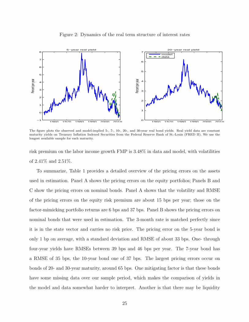
Figure 2: Dynamics of the real term structure of interest rates
1960 1970 1980 1990 2000 2010−1
0
1
2
3
4
5
6
7
8
Perce
nt per y
ear
5−year real yield
1960 1970 1980 1990 2000 20100
1
2
3
4
5
6
7
Perce
nt per y
ear
20−year real yield
modeldata
The figure plots the observed and model-implied 5-, 7-, 10-, 20-, and 30-year real bond yields. Real yield data are constantmaturity yields on Treasury Inflation Indexed Securities from the Federal Reserve Bank of St.-Louis (FRED II). We use thelongest available sample for each maturity.
risk premium on the labor income growth FMP is 3.48% in data and model, with volatilities
of 2.41% and 2.51%.
To summarize, Table 1 provides a detailed overview of the pricing errors on the assets
used in estimation. Panel A shows the pricing errors on the equity portfolios; Panels B and
C show the pricing errors on nominal bonds. Panel A shows that the volatility and RMSE
of the pricing errors on the equity risk premium are about 15 bps per year; those on the
factor-mimicking portfolio returns are 6 bps and 37 bps. Panel B shows the pricing errors on
nominal bonds that were used in estimation. The 3-month rate is matched perfectly since
it is in the state vector and carries no risk price. The pricing error on the 5-year bond is
only 1 bp on average, with a standard deviation and RMSE of about 33 bps. One- through
four-year yields have RMSEs between 39 bps and 46 bps per year. The 7-year bond has
a RMSE of 35 bps, the 10-year bond one of 37 bps. The largest pricing errors occur on
bonds of 20- and 30-year maturity, around 65 bps. One mitigating factor is that these bonds
have some missing data over our sample period, which makes the comparison of yields in
the model and data somewhat harder to interpret. Another is that there may be liquidity
25
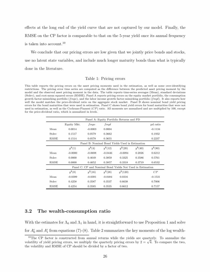
effects at the long end of the yield curve that are not captured by our model. Finally, the
RMSE on the CP factor is comparable to that on the 5-year yield once its annual frequency
is taken into account.10
We conclude that our pricing errors are low given that we jointly price bonds and stocks,
use no latent state variables, and include much longer maturity bonds than what is typically
done in the literature.
Table 1: Pricing errors
This table reports the pricing errors on the asset pricing moments used in the estimation, as well as some over-identifyingrestrictions. The pricing error time series are computed as the difference between the predicted asset pricing moment by themodel and the observed asset pricing moment in the data. The table reports time-series averages (Mean), standard deviations(Stdev), and root-mean squared errors (RMSE). Panel A reports pricing errors on the equity market portfolio, the consumptiongrowth factor-mimicking portfolio (fmpc), and the labor income growth factor-mimicking portfolio (fmpl). It also reports howwell the model matches the price-dividend ratio on the aggregate stock market. Panel B shows nominal bond yield pricingerrors for the bond maturities that were used in estimation. Panel C shows bond yield errors for bond maturities that were notused in estimation, as well as the Cochrane-Piazzesi (CP ) ratio. All moments are annualized and are multiplied by 100, exceptfor the price-dividend ratio, which is annualized in levels.
Panel A: Equity Portfolio Returns and PD
Equity Mkt. fmpc fmpl pd ratio
Mean 0.0014 -0.0003 0.0004 -0.1134
Stdev 0.1517 0.0579 0.3662 0.1932
RMSE 0.1514 0.0578 0.3655 0.2237
Panel B: Nominal Bond Yields Used in Estimation
y$(1) y$(4) y$(12) y$(20) y$(40) y$(80)
Mean -0.0000 -0.0698 -0.0446 -0.0094 0.2026 0.6212
Stdev 0.0000 0.4649 0.3859 0.3325 0.3586 0.5761
RMSE 0.0000 0.4652 0.3857 0.3318 0.3719 0.6532
Panel C: CP and Nominal Bond Yields Not Used in Estimation
y$(8) y$(16) y$(28) y$(120) CP
Mean -0.0399 -0.0391 -0.0484 0.0316 -0.1531
Stdev 0.4258 0.3587 0.3537 0.6638 0.7006
RMSE 0.4254 0.3585 0.3535 0.6612 0.7157
3.2 The wealth-consumption ratio
With the estimates for Λ0 and Λ1 in hand, it is straightforward to use Proposition 1 and solve
for Ac0 and Ac
1 from equations (7)-(8). Table 2 summarizes the key moments of the log wealth-
10The CP factor is constructed from annual returns while the yields are quarterly. To annualize thevolatility of yield pricing errors, we multiply the quarterly pricing errors by 2 =
√4. To compare the two,
the volatility and RMSE of CP should be divided by a factor of two.
26

consumption ratio obtained in quarterly data in column 3. The numbers in parentheses
are small sample bootstrap standard errors, computed using the procedure described in
Appendix B.9.
3.2.1 Comparison to stocks
We can directly compare the moments of the wealth-consumption ratio with those of the
price-dividend ratio on equity. The wc ratio has an annualized volatility of 19% in the data,
considerably lower than the 29% volatility of the pdm ratio. The wc ratio in the data is
a persistent process; its 1-quarter (4-quarter) serial correlation is .97 (.87). This is similar
to the .94 (.77) serial correlation of pdm. The annual volatility of changes in the wealth
consumption ratio is 4.51%, and because of the low volatility of aggregate consumption
growth changes, this translates into a volatility of the total wealth return on the same order
of magnitude (4.59%). The corresponding annual volatility of 9.2% is about half the 17.2%
volatility of stock returns. The change in the wc ratio and the total wealth return have
weak autocorrelation, suggesting that total wealth returns are hard to forecast by their own
lags. The correlation between the (quarterly) total wealth return and consumption growth
is mildly positive (.21).
How risky is total wealth compared to equity? According to our estimation, the con-
sumption risk premium (calculated from equation 11) is 60 bps per quarter or 2.38% per
year. This results in a mean wealth-consumption ratio of 5.81 in logs (Ac0), or 83 in annual
levels (expAc0− log(4)). The consumption risk premium is only one-third as big as the eq-
uity risk premium of 6.41%. Correspondingly, the wealth-consumption ratio is much higher
than the price-dividend ratio on equity: 83 versus 26. A simple back-of-the-envelope Gordon
growth model calculation sheds light on the mean of the wealth-consumption ratio. The
discount rate on the consumption claim is 3.51% per year (a consumption risk premium of
2.38% plus a risk-free rate of 1.49% minus a Jensen term of 0.37%) and its cash-flow growth
rate is 2.31%: 83 = 1/(.0351− .0231). The standard errors on the moments of the wealth-
27
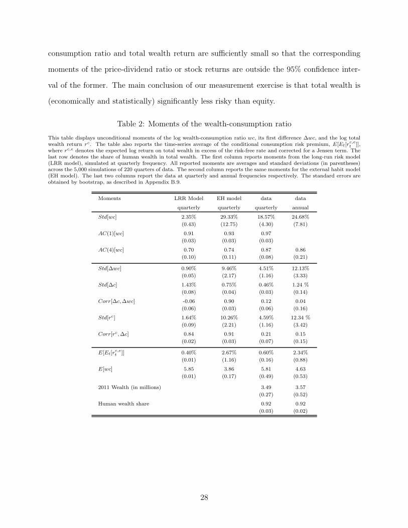
consumption ratio and total wealth return are sufficiently small so that the corresponding
moments of the price-dividend ratio or stock returns are outside the 95% confidence inter-
val of the former. The main conclusion of our measurement exercise is that total wealth is
(economically and statistically) significantly less risky than equity.
Table 2: Moments of the wealth-consumption ratio
This table displays unconditional moments of the log wealth-consumption ratio wc, its first difference ∆wc, and the log totalwealth return rc. The table also reports the time-series average of the conditional consumption risk premium, E[Et[r
c,et ]],
where rc,e denotes the expected log return on total wealth in excess of the risk-free rate and corrected for a Jensen term. Thelast row denotes the share of human wealth in total wealth. The first column reports moments from the long-run risk model(LRR model), simulated at quarterly frequency. All reported moments are averages and standard deviations (in parentheses)across the 5,000 simulations of 220 quarters of data. The second column reports the same moments for the external habit model(EH model). The last two columns report the data at quarterly and annual frequencies respectively. The standard errors areobtained by bootstrap, as described in Appendix B.9.
Moments LRR Model EH model data data
quarterly quarterly quarterly annual
Std[wc] 2.35% 29.33% 18.57% 24.68%
(0.43) (12.75) (4.30) (7.81)
AC(1)[wc] 0.91 0.93 0.97
(0.03) (0.03) (0.03)
AC(4)[wc] 0.70 0.74 0.87 0.86
(0.10) (0.11) (0.08) (0.21)
Std[∆wc] 0.90% 9.46% 4.51% 12.13%
(0.05) (2.17) (1.16) (3.33)
Std[∆c] 1.43% 0.75% 0.46% 1.24 %
(0.08) (0.04) (0.03) (0.14)
Corr[∆c,∆wc] -0.06 0.90 0.12 0.04
(0.06) (0.03) (0.06) (0.16)
Std[rc] 1.64% 10.26% 4.59% 12.34 %
(0.09) (2.21) (1.16) (3.42)
Corr[rc,∆c] 0.84 0.91 0.21 0.15
(0.02) (0.03) (0.07) (0.15)
E[Et[rc,et ]] 0.40% 2.67% 0.60% 2.34%
(0.01) (1.16) (0.16) (0.88)
E[wc] 5.85 3.86 5.81 4.63
(0.01) (0.17) (0.49) (0.53)
2011 Wealth (in millions) 3.49 3.57
(0.27) (0.52)
Human wealth share 0.92 0.92
(0.03) (0.02)
28

3.2.2 Comparison to claim to trend consumption
The claim to trend consumption is the second benchmark for the risky consumption claim.
Table 3 reports the same moments as Table 2 but for a claim to deterministically growing
consumption. We estimate a risk premium on the trend claim of 64 bps per quarter or 2.58%
per annum. The difference with the consumption risk premium is 4 bps per quarter and not
statistically different from zero. Because the claims to risky and to trend consumption differ
only in terms of their consumption cash flow risk, the small difference in risk premia shows
that the market assigns essentially zero compensation to current consumption innovations.
This is the result of two offsetting forces. One the one hand, quarterly consumption inno-
vations are positively correlated to market equity and consumption FMP portfolio shocks,
both of which carry a positive price of risk. This equity exposure adds to the consumption
risk premium. On the other hand, quarterly consumption innovations hedge both shocks to
the level (second orthogonalized shock) and the slope (fourth orthogonalized shock) of the
term structure. Consumption innovations are positively correlated with level innovations,
which carry a negative risk price, and they are negatively correlated with slope shocks, which
carry a positive risk price. Both of these term structure exposures lower the consumption
risk premium. Put differently, the claim to trend consumption has a higher exposure to
interest rate shocks than the claim to risky consumption because of the interest rate hedging
benefits of the latter. Exposure to stock market risk (almost) offsets the lower bond market
risk exposure so that the two claims end up with nearly the same risk premium.
3.2.3 Dividend and high-volatility consumption claim
The different volatility of the consumption and dividend claims cannot account for the dif-
ference between the average consumption and equity risk premium, but it can help to un-
derstand the difference in their dynamics. We price a claim to “high-volatility consumption”
with cash flow growth given by µc+ ae′cΨzt+ ae′cΣ12εt+1, where the scalar a = 5.5 makes the
unconditional variance equal to that of the dividend claim. The annual mean risk premium
29
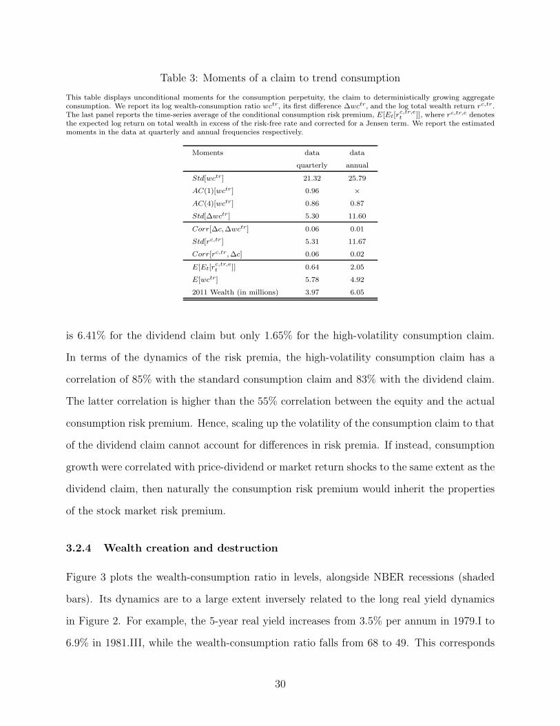
Table 3: Moments of a claim to trend consumption
This table displays unconditional moments for the consumption perpetuity, the claim to deterministically growing aggregateconsumption. We report its log wealth-consumption ratio wctr, its first difference ∆wctr, and the log total wealth return rc,tr.The last panel reports the time-series average of the conditional consumption risk premium, E[Et[r
c,tr,et ]], where rc,tr,e denotes
the expected log return on total wealth in excess of the risk-free rate and corrected for a Jensen term. We report the estimatedmoments in the data at quarterly and annual frequencies respectively.
Moments data data
quarterly annual
Std[wctr] 21.32 25.79
AC(1)[wctr] 0.96 ×
AC(4)[wctr] 0.86 0.87
Std[∆wctr] 5.30 11.60
Corr[∆c,∆wctr] 0.06 0.01
Std[rc,tr] 5.31 11.67
Corr[rc,tr,∆c] 0.06 0.02
E[Et[rc,tr,et ]] 0.64 2.05
E[wctr] 5.78 4.92
2011 Wealth (in millions) 3.97 6.05
is 6.41% for the dividend claim but only 1.65% for the high-volatility consumption claim.
In terms of the dynamics of the risk premia, the high-volatility consumption claim has a
correlation of 85% with the standard consumption claim and 83% with the dividend claim.
The latter correlation is higher than the 55% correlation between the equity and the actual
consumption risk premium. Hence, scaling up the volatility of the consumption claim to that
of the dividend claim cannot account for differences in risk premia. If instead, consumption
growth were correlated with price-dividend or market return shocks to the same extent as the
dividend claim, then naturally the consumption risk premium would inherit the properties
of the stock market risk premium.
3.2.4 Wealth creation and destruction
Figure 3 plots the wealth-consumption ratio in levels, alongside NBER recessions (shaded
bars). Its dynamics are to a large extent inversely related to the long real yield dynamics
in Figure 2. For example, the 5-year real yield increases from 3.5% per annum in 1979.I to
6.9% in 1981.III, while the wealth-consumption ratio falls from 68 to 49. This corresponds
30
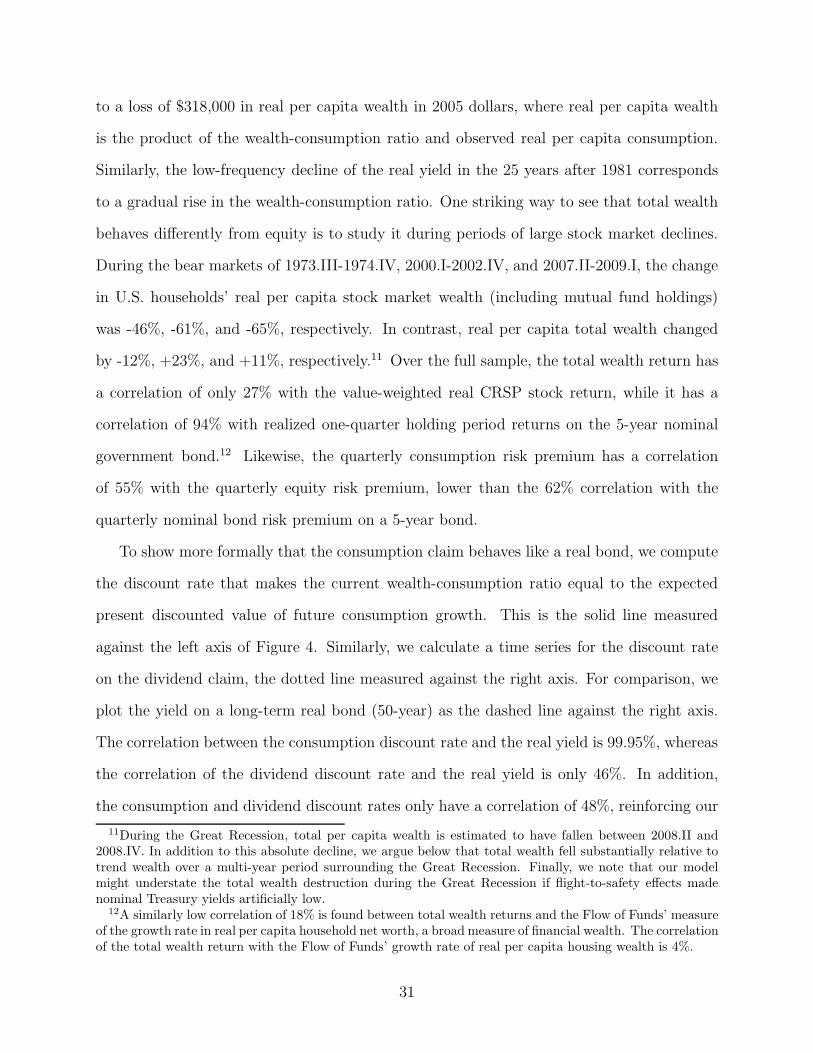
to a loss of $318,000 in real per capita wealth in 2005 dollars, where real per capita wealth
is the product of the wealth-consumption ratio and observed real per capita consumption.
Similarly, the low-frequency decline of the real yield in the 25 years after 1981 corresponds
to a gradual rise in the wealth-consumption ratio. One striking way to see that total wealth
behaves differently from equity is to study it during periods of large stock market declines.
During the bear markets of 1973.III-1974.IV, 2000.I-2002.IV, and 2007.II-2009.I, the change
in U.S. households’ real per capita stock market wealth (including mutual fund holdings)
was -46%, -61%, and -65%, respectively. In contrast, real per capita total wealth changed
by -12%, +23%, and +11%, respectively.11 Over the full sample, the total wealth return has
a correlation of only 27% with the value-weighted real CRSP stock return, while it has a
correlation of 94% with realized one-quarter holding period returns on the 5-year nominal
government bond.12 Likewise, the quarterly consumption risk premium has a correlation
of 55% with the quarterly equity risk premium, lower than the 62% correlation with the
quarterly nominal bond risk premium on a 5-year bond.
To show more formally that the consumption claim behaves like a real bond, we compute
the discount rate that makes the current wealth-consumption ratio equal to the expected
present discounted value of future consumption growth. This is the solid line measured
against the left axis of Figure 4. Similarly, we calculate a time series for the discount rate
on the dividend claim, the dotted line measured against the right axis. For comparison, we
plot the yield on a long-term real bond (50-year) as the dashed line against the right axis.
The correlation between the consumption discount rate and the real yield is 99.95%, whereas
the correlation of the dividend discount rate and the real yield is only 46%. In addition,
the consumption and dividend discount rates only have a correlation of 48%, reinforcing our
11During the Great Recession, total per capita wealth is estimated to have fallen between 2008.II and2008.IV. In addition to this absolute decline, we argue below that total wealth fell substantially relative totrend wealth over a multi-year period surrounding the Great Recession. Finally, we note that our modelmight understate the total wealth destruction during the Great Recession if flight-to-safety effects madenominal Treasury yields artificially low.
12A similarly low correlation of 18% is found between total wealth returns and the Flow of Funds’ measureof the growth rate in real per capita household net worth, a broad measure of financial wealth. The correlationof the total wealth return with the Flow of Funds’ growth rate of real per capita housing wealth is 4%.
31
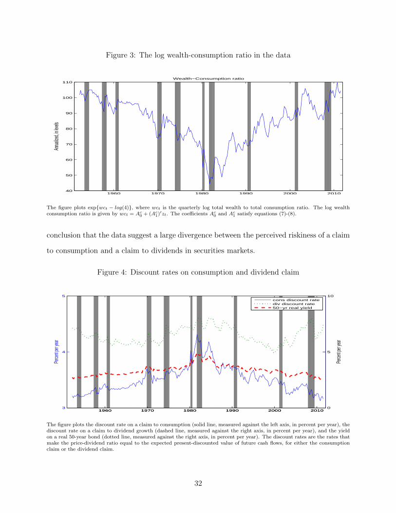
Figure 3: The log wealth-consumption ratio in the data
Wealth−Consumption ratio
Annua
lized, i
n level
s
1960 1970 1980 1990 2000 201040
50
60
70
80
90
100
110
The figure plots expwct − log(4), where wct is the quarterly log total wealth to total consumption ratio. The log wealthconsumption ratio is given by wct = Ac
0 + (Ac1)
′zt. The coefficients Ac0 and Ac
1 satisfy equations (7)-(8).
conclusion that the data suggest a large divergence between the perceived riskiness of a claim
to consumption and a claim to dividends in securities markets.
Figure 4: Discount rates on consumption and dividend claim
Perce
nt pe
r yea
r
1960 1970 1980 1990 2000 20103
4
5
1960 1970 1980 1990 2000 20100
5
10
Perce
nt pe
r yea
r
cons discount ratediv discount rate50−yr real yield
The figure plots the discount rate on a claim to consumption (solid line, measured against the left axis, in percent per year), thediscount rate on a claim to dividend growth (dashed line, measured against the right axis, in percent per year), and the yieldon a real 50-year bond (dotted line, measured against the right axis, in percent per year). The discount rates are the rates thatmake the price-dividend ratio equal to the expected present-discounted value of future cash flows, for either the consumptionclaim or the dividend claim.
32
A second way of showing that the consumption claim is bond-like is to study yields on
consumption strips. We decompose the yield on the period-τ strip into two components.
The first component is the yield on a security that pays a certain cash flow (1 + µc)τ .
The underlying security is a real perpetuity with a cash flow that grows at a deterministic
consumption growth rate, µc. The second component is the yield on a security that pays off
Cτ/C0 − (1 + µc)τ ; it captures pure consumption cash flow risk. Appendix B.4 shows that
the log price-dividend ratios on the consumption strips are approximately affine in the state,
and details how to compute the yield on its two components. In our model, consumption
strip yields are mostly comprised of a compensation for variation in real rates (labeled “real
bond yield -µc” in Figure B.5), not consumption cash flow risk (labeled “yccr”). Other than
at short horizons, the consumption cash flow risk security has a yield that is approximately
zero.
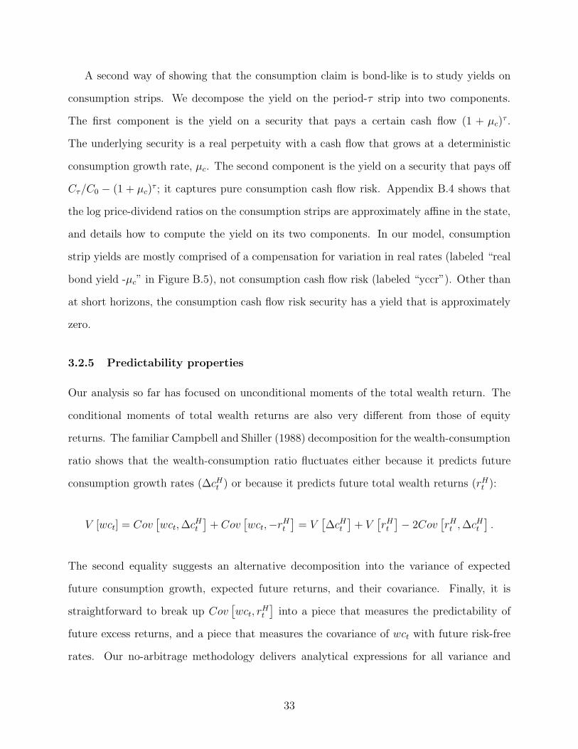
3.2.5 Predictability properties
Our analysis so far has focused on unconditional moments of the total wealth return. The
conditional moments of total wealth returns are also very different from those of equity
returns. The familiar Campbell and Shiller (1988) decomposition for the wealth-consumption
ratio shows that the wealth-consumption ratio fluctuates either because it predicts future
consumption growth rates (∆cHt ) or because it predicts future total wealth returns (rHt ):
V [wct] = Cov[wct,∆cHt
]+ Cov
[wct,−rHt
]= V
[∆cHt
]+ V
[rHt
]− 2Cov
[rHt ,∆cHt
].
The second equality suggests an alternative decomposition into the variance of expected
future consumption growth, expected future returns, and their covariance. Finally, it is
straightforward to break up Cov[wct, r
Ht
]into a piece that measures the predictability of
future excess returns, and a piece that measures the covariance of wct with future risk-free
rates. Our no-arbitrage methodology delivers analytical expressions for all variance and
33

covariance terms (See Appendix B). Table 4 reports the complete variance decomposition of
the wc and pdm ratios into the three variance terms and the three covariances (top panel)
and into the three covariance terms (bottom panel), under our benchmark calibration.
We draw four main empirical conclusions. First, the mild variability of the wc ratio im-
plies only mild total wealth return predictability. This is in contrast with the high variability
(and predictability) of pdm. Second, 104.9% of the variability in wc is due to covariation
with future total wealth returns, while the remaining -4.9% is due to covariation with future
consumption growth. Hence, the wealth-consumption ratio predicts future returns (discount
rates), not future consumption growth rates (cash flows). Using the second variance decom-
position, the variability of future returns is 111.5%, the variability of future consumption
growth is 1.7% and their covariance is -13.2% of the total variance of wc. This variance
decomposition is similar to the one for equity. Third, 77.5% of the 104.9% covariance with
returns is due to covariance with future risk-free rates, and the remaining 27.4% is due to co-
variance with future excess returns. The wealth-consumption ratio therefore mostly predicts
future variation in interest rates, not in risk premia. The exact opposite holds for equity: the
bulk of the predictability of the pdm ratio for future stock returns is predictability of excess
returns (50.4% out of 66.5%). Fourth, though modest in both cases, variation in expected
future cash-flow growth is more important for the equity claim than for the consumption
claim. In sum, the conditional asset pricing moments also reveal interesting differences be-
tween equity and total wealth. Again, they point to the strong link between the consumption
claim return and interest rates.
3.3 Human wealth returns
Our estimates indicate that the bulk of total wealth is human wealth. The human wealth
share fluctuates between 86% and 99%, with an average of 92% (see last row of Table 2).
Interestingly, Jorgenson and Fraumeni (1989) calculates a similar 90% human wealth share.
The average price-dividend ratios on human wealth is slightly above the one on total wealth
34

Table 4: Variance decomposition wealth-consumption ratio
The first column reports the benchmark wc ratio decomposition; all numbers are multiplied by 100. The second columnexpresses the numbers of the first column as a percentage of the total variability of the wc ratio. The third and fourth columnsare the decomposition of the pdm ratio in actual values (times 100) and in percent, respectively. For these last two columns, itis understood that the notation ∆cHt refers to expected future dividend growth rates.
Moments V [wc] V [pdm]
×100 in % ×100 in %
V[
∆cHt]
0.06 1.65 1.11 13.63
V[
rpHt]
0.71 20.45 3.29 40.33
V[
rfHt
]
2.46 71.39 1.93 23.65
−2Cov[
∆cHt , rpHt]
−0.20 −5.71 3.05 37.43
−2Cov[
∆cHt , rfHt
]
−0.26 −7.47 0.18 2.15
2Cov[
rpHt , rfHt
]
0.68 19.69 −1.40 −17.18
Cov[
∆cHt , wct]
−0.17 −4.94 2.73 33.41
−Cov[
rpHt , wct]
0.95 27.44 4.12 50.45
−Cov[
rfHt , wct
]
2.67 77.50 1.32 16.13
(93 vs. 83 in annual levels). The risk premium on human wealth is very similar to the one
for total wealth (2.31 vs. 2.38% per year). The price-dividend ratios and risk premia on
human wealth and total wealth have a 99.87% (99.95%) correlation.
Existing approaches to measuring total wealth make ad hoc assumptions about expected
human wealth returns. Campbell (1996) assumes that expected human wealth returns are
equal to expected returns on financial assets. This is a natural benchmark when financial
wealth is a claim to a constant fraction of aggregate consumption. Shiller (1995) models
a constant discount rate on human wealth. Jagannathan and Wang (1996) assume that
expected returns on human wealth equal the expected labor income growth rate; the resulting
price-dividend ratio on human wealth is constant. The construction of cay in Lettau and
Ludvigson (2001a) makes that same assumption. Our approach avoids having to make
arbitrary assumptions on unobserved human wealth returns.13
Our estimation results indicate that expected excess human wealth returns have an annual
volatility of 2.9%. This is substantially higher than the volatility of expected labor income
growth (0.6%), but lower than that of the expected excess returns on equity (3.3%). Lastly,
13These models can be thought of as special cases of ours, imposing additional restrictions on the marketprices of risk Λ0 and Λ1. Our work rejects these additional assumptions.
35

average (real) human wealth returns (3.8%) are much lower than (real) equity returns (7.9%),
but higher than (real) labor income growth (2.3%) and the (real) short rate (1.5%).
How much human wealth do our estimates imply? In real 2005 dollars, total per capita
wealth increased from $0.87 million to $3.49 million between 1952 and 2011. The thick solid
line in the left panel of Figure 5 shows the time series. Of this, $3.2 million was human
wealth in 2011 (dashed line in left panel), while the remainder is non-human wealth (solid
line in right panel). To judge whether this is a reasonable number, we compute the fraction
of human wealth that accrues in the first 35 years.14 In 2011, this implies a human wealth
value of $1.04 million per capita (dashed line in the right panel). This amount is the price of
a 35-year annuity with a cash flow of $38,268 that grows at the average labor income growth
rate of 2.31% and is discounted at the average real rate of return on human wealth of 3.81%.
This model-implied annual income of $38,268 compares to U.S. per capital labor income of
$24,337 at the end of 2011. Another reference point for the “first 35 years” human wealth
number is per capita residential home equity from the Flow of Funds. In 2011, home equity
is a factor 51 smaller than human wealth. Unlike the massive destruction of home equity,
human wealth has grown substantially over the last five years and is the main driver behind
the overall wealth accumulation.15
Finally, we compare non-human wealth, the difference between our estimates for total
and for human wealth, with the Flow of Funds series for household net worth. The latter
is the sum of equity, bonds, housing wealth, durable wealth, private business wealth, and
pension and life insurance wealth minus mortgage and credit card debt. Our non-human
wealth series is on average 3.3 times the Flow of Funds series. This ratio varies over time:
it is 10.1 at the beginning and 1.7 at the end of the sample, and it reaches a low of 0.46
in 1975. We chose not to use the Flow of Funds net worth data in our estimation because
14This fraction is the price of the first 140 quarterly labor income strips divided by the price of all laborincome strips. The labor income strip prices are computed just like the consumption strip prices. On average,35% of human wealth pertains to the first 35 years.
15The destruction of housing wealth has been linked to a reversal of a financial market liberalization incredit markets by Favilukis, Ludvigson, and Van Nieuwerburgh (2011). This increased risk premia morethan offsets the large fall in real rates during the Great Recession.
36
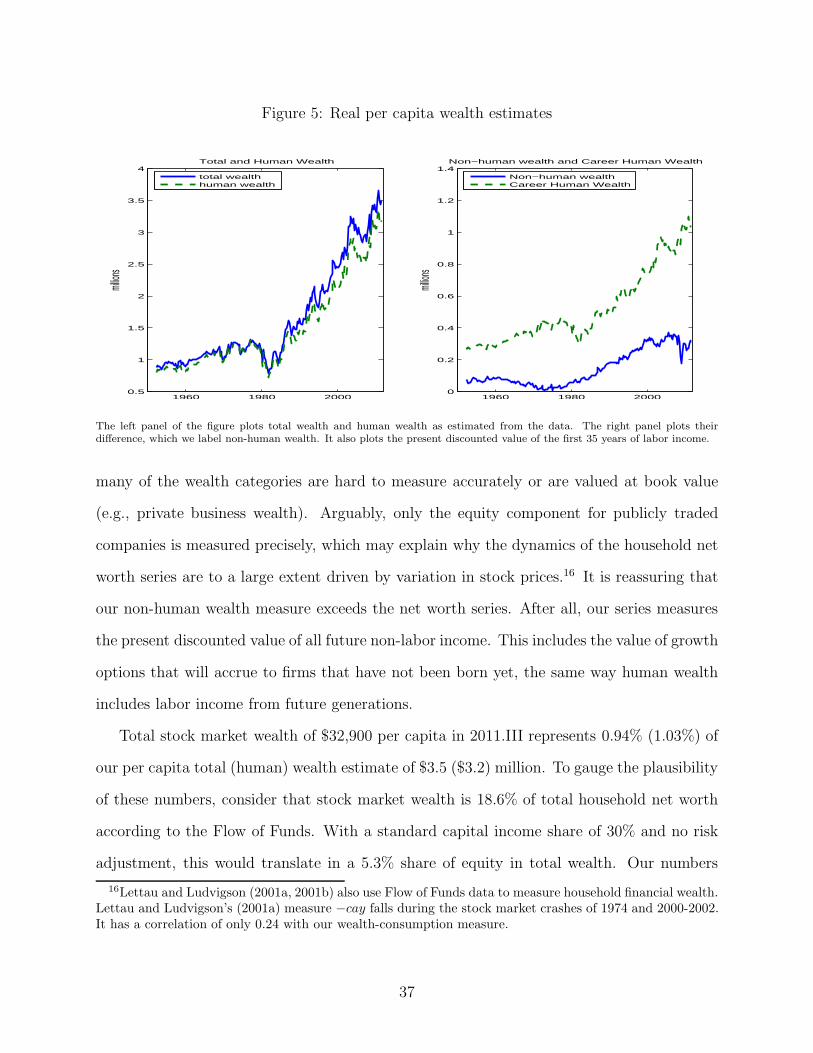
Figure 5: Real per capita wealth estimates
1960 1980 20000.5
1
1.5
2
2.5
3
3.5
4
million
s
Total and Human Wealth
total wealthhuman wealth
1960 1980 20000
0.2
0.4
0.6
0.8
1
1.2
1.4
million
s
Non−human wealth and Career Human Wealth
Non−human wealthCareer Human Wealth
The left panel of the figure plots total wealth and human wealth as estimated from the data. The right panel plots theirdifference, which we label non-human wealth. It also plots the present discounted value of the first 35 years of labor income.
many of the wealth categories are hard to measure accurately or are valued at book value
(e.g., private business wealth). Arguably, only the equity component for publicly traded
companies is measured precisely, which may explain why the dynamics of the household net
worth series are to a large extent driven by variation in stock prices.16 It is reassuring that
our non-human wealth measure exceeds the net worth series. After all, our series measures
the present discounted value of all future non-labor income. This includes the value of growth
options that will accrue to firms that have not been born yet, the same way human wealth
includes labor income from future generations.
Total stock market wealth of $32,900 per capita in 2011.III represents 0.94% (1.03%) of
our per capita total (human) wealth estimate of $3.5 ($3.2) million. To gauge the plausibility
of these numbers, consider that stock market wealth is 18.6% of total household net worth
according to the Flow of Funds. With a standard capital income share of 30% and no risk
adjustment, this would translate in a 5.3% share of equity in total wealth. Our numbers
16Lettau and Ludvigson (2001a, 2001b) also use Flow of Funds data to measure household financial wealth.Lettau and Ludvigson’s (2001a) measure −cay falls during the stock market crashes of 1974 and 2000-2002.It has a correlation of only 0.24 with our wealth-consumption measure.
37

are lower because we find that human wealth is substantially less risky than stock market
wealth, requiring labor income cash flows to be discounted substantially less than equity
dividends.
4 Robustness
4.1 Smaller models
The results of our estimation exercise are robust to different specifications of the law of
motion for the state z. Appendix C.1 considers five alternative models that have fewer state
variables than our benchmark exercise and lists the goodness-of-fit for each of these. The
variations are selected to give insight into what drives our main result. For brevity, we
discuss only the main findings here.
The simplest model (labeled Model 2 in the Appendix C.1) has a simplified term structure
and deliberately ignores any equity moments. Despite its simplicity, it generates a reasonably
good fit to the nominal bond yields, and even to the nominal bond risk premium. It implies
a lower consumption risk premium of 2.11% per year (compared to 2.38% in the benchmark)
and thus a higher mean wealth-consumption ratio of 113 (vs. 83). The wealth-consumption
ratios have a correlation of 99% because the term structure fit of the simple model is com-
parable to that of the benchmark model. The marginal cost of consumption fluctuations,
which averages 36.2%, is substantially higher than in the benchmark model (average of -
2.4%), and the two have a time series correlation of only 63%. The reason for the higher cost
of consumption fluctuations is that there is more consumption cash flow risk in this simple
model. Instead of hedging it as in the benchmark model, consumption cash flow risk adds
interest rate exposure, which increases the consumption risk premium, ceteris paribus. The
lower bond risk premium more than offsets the higher consumption risk so that the overall
consumption risk premium ends up lower than in the benchmark. This model illustrates
that the inverse relationship between real rates and the wealth consumption ratio as well as
38

the low consumption risk premium and high wealth-consumption ratio are generic features
that arise even in a very simple model. But, because it does not price stock-based moments
(by construction), the question is whether or not the low consumption risk premium is the
result of ignoring important sources of risk when pricing the consumption claim. To dispel
this possibility, we consider both bond- and stock-based moments in our benchmark model.
We consider another simple model (labeled Model 3) that prices aggregate equity mo-
ments well but that has only a one-factor term structure. This model has a much worse fit
for bond yields, but a similar mean consumption risk premium of 2.24% and mean wealth-
consumption ratio of 96. The volatility of the wc ratio is lower at 14% and the time series
correlation with the wc ratio of the benchmark is 93.0%, the lowest among all alternative
models we consider. The consumption risk premium only has a correlation of 67% with that
in the benchmark (68% with Model 2), again the lowest among the alternatives. Clearly
consumption risk premium dynamics are substantially affected by giving up on a reasonably
fitting term structure model.
Combining the two simple models results in a better fit (Model 4) but otherwise similar
results. When we add the CP factor to the state and the estimation (Model 5), results change
meaningfully. In particular, the hedging benefits of consumption cash flows can be traced
back to adding the CP factor. The addition of CP results in a large drop of the consumption
risk premium from 53% in Model 4 to -2% in Model 5, on average. The addition of CP
also forces the model to match the 1-year bond risk premium more closely, at the expense
of the long-term bond risk premia and yields. The 20-year nominal bond yield in Model
5, for example, is 27 bps higher than that in Model 4 without CP, translating into a lower
wealth-consumption ratio. The final model is one without CP but with the factor-mimicking
portfolios. That model looks similar to Model 4, except that there is more consumption cash
flow risk priced and the cost of consumption fluctuations is higher.
In sum, the wealth-consumption dynamics are very similar across models and are largely
driven by the similar dynamics of real yields. Insisting on matching the 1-year bond risk
39

premium (the CP factor), leads to consumption that carries a much lower price of risk and
results in higher long-term mean yield estimates. These two effects result in a lower mean
cost of consumption fluctuations, and have offsetting effects on the mean wealth-consumption
ratio. Without the CP factor, our results would indicate a consumption risk premium that
was lower still and a mean wealth-consumption ratio that was higher still, further reinforcing
our conclusions.
4.2 Simpler VAR dynamics
A second set of robustness exercises explores changes to our benchmark results when we
simplify the VAR dynamics. Appendix C.2 explores four different sets of additional zero
restrictions on the matrix Ψ. In particular, we zero out either all non-significant elements of
Ψ, only the non-significant elements in the stock market block, only those in the FMP block,
or only those in the consumption and labor income block. The dynamics of the resulting
wealth-consumption ratios and consumption risk premia are extremely highly correlated
(above 99%) across our benchmark model and these four variations, in large part because
expected consumption growth dynamics and real yield dynamics are so highly correlated.
The cost of consumption fluctuations also have correlations across models above 90% with
the benchmark model. The main difference is in the average wealth-consumption ratio and
risk premia across models rather than in the dynamics. In the last model with the restricted
consumption and labor growth dynamics, we have the lowest mean wealth-consumption ratio
among all models, at 62, and the highest consumption risk premium at 2.94% per year. The
latter remains well below the observed equity risk premium of 6.41%, so that our main
conclusions are unaffected.
In a last robustness exercise (section C.3), we relax the block-diagonal nature of the
Ψ matrix and allow the bond market dynamics in the first four equations of the VAR to
depend on the lagged stock market variables (next four elements). We find qualitatively and
quantitatively similar results to our benchmark case.
40

4.3 Annual estimation
We repeat our analysis at annual frequency. The annual exercise is useful because annual
VAR dynamics may be able to capture lower-frequency correlations between consumption
growth and traded asset prices than the quarterly results.17
The model structure and estimation procedure are identical, except that the short rate
is now the one-year constant maturity bond yield. We find that annual consumption growth
has a significantly positive covariance with stock returns (t-stat is 3.15), which contributes
to a better spanning of annual consumption growth risk by the traded assets than in the
quarterly model. Indeed, our state variables in zt explain 50% of variation in annual ∆ct+1,
compared to 29% in our benchmark quarterly exercise.
The main results from the annual estimation, which are listed in the last column of Table
2, are similar to those of the quarterly model. The consumption risk premium is nearly
identical at 2.34% (vs. 2.38%). The mean wealth-consumption ratio is 103 compared to an
annualized number of 83 in the benchmark results. The dynamics of the wealth-consumption
ratio still mirror those of long-term real bond yields. Our main message that the consumption
claim is much less risky than equity remains unaffected. The human wealth share is 92%,
just as in the quarterly benchmark.
The main difference with the quarterly results is a much higher marginal cost of con-
sumption fluctuations. The latter is 34% on average in the annual model compared to the
quarterly model where we found a small negative cost. The high cost arises because the risk
premium of the trend consumption claim is substantially lower than that of the risky claim
(2.05% vs. 2.34%), leading to a much higher mean trend wealth-consumption ratio (Table
3). The difference with the quarterly results can be traced back to differences in annual ver-
sus quarterly consumption dynamics. In annual data, consumption innovations have strong
negative correlation with the level (second orthogonal) shock and a less negative correlation
17While it would be interesting to go back to the Great Depression, the necessary bond yield data are notavailable prior to 1953, so that the annual sample spans the same 1952-2011 period as our quarterly sample.
41
with the slope (fourth orthogonal) shock. Both exposures increase the consumption risk
premium above that in the quarterly model. Basically, consumption cash flow shocks no
longer hedge interest rate risk but rather contribute to the interest rate risk that is already
present through the discount rate (the same risk the consumption trend is also exposed to).
Despite the mean differences, the dynamics of the cost of consumption fluctuations are sim-
ilar between annual and quarterly models. The annual series also shows a large destruction
of wealth relative to trend during the Great Recession. These dynamics results from similar
interest rate behavior and from similar deviations of consumption from its trend.
5 Cost of Consumption Risk, Wealth Effects, and Non-
Traded Risk
In this section, we explore the economic implications of our measurement exercise. Section
5.1 links the wealth-consumption ratio to the cost of aggregate consumption risk and Section
5.2 links it to the propensity to consume out of wealth. Section 5.3 relaxes the spanning
assumption and proposes bounds on the non-traded consumption risk premium in our model.
5.1 Cost of consumption risk
The computation of the wealth-consumption ratio implies an estimate of the marginal welfare
cost of aggregate consumption growth risk, a central object of interest in this paper. Alvarez
and Jermann (2004) define the marginal cost of consumption uncertainty by how much
consumption the representative agent would be willing to give up at the margin in order
to eliminate some consumption uncertainty.18 Since our approach is preference-free, our
18The literature on the costs of consumption fluctuations starts with Lucas (1987), who defines the total
cost of aggregate consumption risk Ω as the fraction of consumption the consumer is willing to give up inorder to get rid of consumption uncertainty: U
((1 + Ω(α))Cactual
)= U
((1− α)Ctrend + αCactual
), where
α=0. Alvarez and Jermann (2004) define the marginal cost of business cycles as the derivative of this costevaluated at zero, i.e., Ω′(0). While the total cost can only be computed by specifying preferences, themarginal cost can be backed out directly from traded asset prices.
42

marginal cost calculation applies to the entire class of representative agent dynamic asset
pricing models.
Eliminating exposure to aggregate consumption growth risk is achieved by selling a claim
to stochastically growing aggregate consumption and buying a claim to deterministically
growing aggregate consumption. Denote trend consumption by Ctrt . The marginal cost
of consumption uncertainty, t, is defined as the ratio of the price of a claim to trend
consumption (without cash-flow risk) to the price of a claim to consumption with cash-flow
risk minus one:
t =W tr
t
Wt
− 1 =WCtr
t
WCt
Ctrt
Ct
− 1 = ewctrt +ctrt +wct−ct − 1, (13)
where wctr denotes the log price-dividend ratio on the claim to trend consumption, a per-
petuity with cash-flows that grow deterministically at the average real consumption growth
rate, µc. The latter is approximately affine in the state variables: wctrt ≃ Atr0 + Atr′
1 zt (see
Appendix B for a derivation). The risk premium on a claim to trend consumption is not
zero but it approximately equals the risk premium on the real perpetuity:
Et
[rtr,et+1
]≡ Et
[rtrt+1 − yt(1)
]+
1
2Vt[r
trt+1] ≃ Atr′
1 Σ12
(Λ0 − Σ
12′eπ
)+ Atr′
1 Σ12Λ1zt. (14)
The marginal cost of business cycles is zero, on average, when innovations to current and
future consumption growth jointly carry a zero price of risk, so that wct ≈ wctrt . Even in
the latter case, the marginal cost of consumption fluctuations will fluctuate because realized
consumption is at times above and at times below trend.
Figure 6 shows the cost of consumption fluctuations () in our benchmark model. It
breaks down this cost into the ratio of the wealth-consumption ratios of the trend claim to
that of the risky consumption claim and the ratio of trend consumption to consumption (see
equation 13). The average cost of consumption fluctuations is slightly negative, consistent
with the slightly lower consumption risk premium arising from the hedging properties of
43

consumption discussed above.
Figure 6: Cost of consumption fluctuations
Cos
t of C
onsu
mpt
ion
Fluc
tuat
ions
− In
Per
cent
1960 1970 1980 1990 2000 2010−20
0
20
1960 1970 1980 1990 2000 20100.8
1
1.2
Rat
ios
Cost of Consumption FluctuationsWC trend/WCC trend/C
The figure plots the marginal cost of consumption fluctuations t =W tr
t
Wt
− 1 =WCtr
t
WCt
Ctr
t
Ct
− 1 against the left axis (solid line).
It also plots the two ratio termsWCtr
t
WCt
(dotted line) andCtr
t
Ct
(dashed line) that constitute t.
More interesting than the mean is the substantial amount of variation in the marginal
cost. At the end of the sample, the cost of consumption fluctuations skyrockets. This
happens because consumption is far below trend and because the ultra-low interest rates
result in a much higher trend WC ratio than risky WC ratio (recall the former’s greater
interest rate sensitivity). In other words, total wealth falls far below trend during the Great
Recession. Thus, relative to trend, our model implies a large wealth destruction during the
Great Recession.
44

5.2 Propensity to consume out of wealth
A large literature studies households’ average and marginal propensities to consume out
of wealth. To the best of our knowledge, ours is the first estimator of these propensities
that is consistent with both the budget constraint and no-arbitrage pricing of stock and
bond prices. Specifically, the consumption-wealth ratio evaluated at the sample average
state vector, exp (−Ac0), is a no-arbitrage estimate of the average propensity to consume out
of total wealth. We also obtain the marginal propensity to consume out of total wealth:
(1+ e′cAc1)
−1 exp (− (Ac0 + Ac′
1 zt)).19 The dynamics of the marginal cost of consumption fluc-
tuations vary directly with the consumption-wealth ratio.
The average propensity to consume out of total wealth in our benchmark estimation is 1.2
cents for every dollar of wealth (= 1/83). The marginal propensity to consume out of (the
last dollar increase in) total wealth is 0.75 cents. Our estimates for the marginal propensity
are at the low end of the range of numbers in the literature (Poterba 2000).20 In contrast, if
the consumption claim was priced like equity, the average propensity to consume would be
much higher: 3.9 cents (1/26) out of every dollar. Such a number is in the ballpark of the 5
cent estimate that is suggested by Modigliani (1971) and a large literature that follows it.
There is considerable variation in the marginal propensity to consume. It peaks at 1.40
cents per dollar in 1981.IV, when real interest rates peak, and it bottoms out at 0.57 cents
in 2010.IV, when real interest rates bottom out. The 50% decline in the propensity to
consume occurs despite the massive wealth creation over the 1981 to 2010 period. The logic
of the budget constraint imposes that the propensity to consume must drop when expected
total wealth returns drop. The latter are highly correlated with real interest rates, which
19In the literature, the marginal propensity to consume is the slope coefficient a1 in the following regression:∆ct+1 = a0 + a1∆wt+1 + ǫt+1. From our estimates, we can back out the implied marginal propensity toconsume as follows: a−1
1 = ∂(∆wt+1)/∂(∆ct+1) = ∂(∆wct+1 +∆ct+1)/∂(∆ct+1) = ∂(∆wct+1)/∂(∆ct+1) +1 = e′
cAc
1 + 1. We multiply a1 = (e′cAc
1 + 1)−1 by the consumption-wealth ratio to get an expression of themarginal propensity to consume out of wealth in levels (cents per dollars).
20In part this is because we consider total wealth, the infinite present discounted value of all future laborand dividend income. If we were to limit ourselves to a 35-year “career” for labor income, the marginalpropensity to consume would be three times higher at 2.3 cents per last dollar of career human wealth.
45

fall substantially over this period. Our estimated decline is consistent with Ludvigson and
Steindel (1999), who report a large drop in the marginal propensity to consume out of stock
market wealth after 1986.
Time variation in the wealth-consumption ratio implies that the wealth effect decreases
during periods of abnormal total wealth creation, while it increases during periods of ab-
normal total wealth destruction. Previously, Poterba (2000) and others had speculated that
consumers may respond more strongly to wealth destruction than creation. Moreover, macro-
economists have long been puzzled by the dramatic destruction of capital in 1973 and 1974,
inferred from the stock market’s steep decline s (e.g. Hall 2001). Our findings suggest these
events in the stock market only had a minor impact on total U.S. wealth, and are consistent
with Hobijn and Jovanovic’s (2001) account of this episode.
5.3 Non-traded consumption risk
So far we have assumed that all aggregate shocks are spanned by stock and bond prices.
This assumption is satisfied in all structural dynamic asset pricing models that we are aware
of. Even in incomplete markets models, asset prices will reflect changes in the income or
wealth distribution (e.g. Constantinides and Duffie 1996).
In the absence of spanning, it is impossible to conclusively bound the wealth-consumption
ratio, except by writing down a fully specified general equilibrium model. However, it is
possible to put reasonable bounds on the non-traded consumption risk premium in our model.
In particular, we relax our assumption that traded assets span all aggregate shocks by freeing
up the 9th element of Λ0, the risk price of the non-traded consumption growth shock that is
orthogonal to the eight traded asset shocks. Table 5 reports the consumption risk premium
(Column 2), the average wealth-consumption ratio (Column 3), the maximum conditional
Sharpe ratio (Column 4,) and the Sharpe ratio on a one-period ahead consumption strip
(Column 5) for different values of the price of non-traded consumption risk, governed by
the 9th-element of Λ0 (Column 1). This parameter does not affect the prices of any traded
46

assets, so this exercise does not change any of the model’s implications for observables.21
The first row in Table 5 reports our benchmark case in which the non-traded consumption
risk is not priced. The consumption risk premium is 2.38% per annum, the maximum Sharpe
ratio is 0.6, and the conditional Sharpe ratio on the one-period ahead consumption strip is .06.
Increasing Λ0(9) increases the consumption risk premium, lowers the wealth-consumption
ratio, and increases the Sharpe ratio on the consumption strip. How far should we increase
Λ0(9)? A first answer is to bound the maximal Sharpe ratio (stdt[mt+1]). Cochrane and
Saa-Requejo (2000) and Alvarez and Jermann (2004) choose a “good deal” bound of one,
which they argue is high because it is twice the 0.5 Sharpe ratio on equities in the data.22
Since we work with quarterly log returns, the Sharpe ratio on equities is only 0.19, and that
same good deal bound of one is more than twice as conservative. This bound is reached
for Λ0(9) around 0.8, and implies a consumption risk premium of 3.91% per annum and an
average wealth-consumption ratio of 36. Even then, the consumption risk premium is still
2.5% short of the equity premium, so that our conclusion that total wealth has different
risk-return characteristics than equity remains valid. In order to match the equity premium
by increasing the price of non-traded consumption risk, we would need an increase in the
maximum Sharpe ratio to twice the good-deal bound or ten times the Sharpe ratio on equity.
This does not seem reasonable for two reasons. First, such non-traded risk would certainly
differ across households and would beg the question of why no market exists to share this risk.
Second, a high risk premium on total consumption would imply a low wealth-consumption
ratio, which in turn would suggest an extremely high marginal cost of business cycles.
A second answer would be to evaluate the Sharpe ratios on the consumption strip return
21Freeing up Λ0(9) also affects the risk premium and price-dividend ratio on human wealth, in quantita-tively similar ways. We also experimented with freeing up the price of risk on the shock to labor incomegrowth that is orthogonal to all previous shocks, including the aggregate consumption growth shock. In-creasing this Λ0(10) has no effect on the consumption risk premium and the wealth-consumption ratio. Itonly affects the risk premium on human wealth. Quantitatively, the effects are similar to those presented inTable 5. The same is true when we simultaneously increase Λ0(9) and Λ0(10).
22In related work, Bernardo and Ledoit (2000) bound the gain-loss ratio, which summarizes the attrac-tiveness of a zero-price portfolio. It is equivalent to a restriction on admissible pricing kernels, precludingthe existence of arbitrage and approximate arbitrage opportunities.
47

in Column 5. When we set Λ0(9) to 0.1, this Sharpe ratio doubles compared to Λ0(9) = 0,
i.e., the implied price of non-traded consumption cash flow risk is much higher than that of
traded consumption cash flow risk on a per unit of risk basis. Allowing the consumption
strip to have the same Sharpe ratio as equity (0.19), would imply a value for Λ0(9) around
0.10. At this value, the consumption risk premium is only about 0.2% per year higher than
in our benchmark case. At Λ0(9) = 0.8, the conditional Sharpe ratio on the consumption
strip is 0.8, four times higher than the Sharpe ratio on equity and 13 times higher than the
Sharpe ratio on the traded consumption strip.
Table 5: Non-traded consumption risk
The first column reports the market price of risk Λ0(9) that is associated with the innovation to consumption growth thatis orthogonal to all innovations to the preceding stock and bond innovations. The second column reports the consumptionrisk premium. The third column reports the average wealth/consumption ratio. The fourth column is the maximum Sharperatio computed as
√
Λ′
0Λ0. The last column shows the conditional Sharpe ratio on a one-period ahead consumption strip:(
e′cΣ1/2Λ0
)
/√
e′cΣ1/2Σ1/2′ec.
Λ0(9) cons. risk premium E[WC] stdt(mt+1) SR on strips
0 2.38% 85 0.58 0.06
0.05 2.48% 78 0.58 0.10
0.10 2.57% 73 0.59 0.15
0.50 3.33% 46 0.77 0.52
0.80 3.91% 36 0.99 0.80
1.00 4.30% 31 1.16 0.98
1.50 5.29% 24 1.61 1.45
2.00 6.30% 19 2.08 1.91
3.00 8.35% 14 3.06 2.84
Finally, Appendix D shows that our methodology for pricing aggregate consumption and
labor income claims remains valid if the data are generated from an economy inhabited by
heterogeneous agents who face idiosyncratic labor income risk, which they cannot perfectly
insure away and who may face binding borrowing or asset market participation constraints.
48

6 Structural Models
We end the paper with a short comparison of our results to those implied by leading asset
pricing models.23 We focus on the long-run risk (LRR) model of Bansal and Yaron (2004)
and the external habit (EH) model of Campbell and Cochrane (1999), each of which has
received an enormous amount of attention in the modern asset pricing literature. Just like
in the affine model we estimated, the log wealth-consumption ratio is linear in the state
variables in each of these two models. We do not attempt to formally test the two models,
only to point out their implications for the wealth-consumption ratio.24 Interestingly, they
have quite different implications for the wealth-consumption ratio. We refer the reader to the
NBER working paper version of our work for a detailed derivation of the wealth-consumption
ratios in these two models and a description of our simulations. We present our main findings
in Columns 1 and 2 of Table 2.
The LRR model produces a wc ratio that matches many features of the data. It is high
on average and not very volatile. For the standard calibration of the LRR model, the mean
annual wealth-consumption ratio is 87, very close to our estimate in the data (eAc,LRR0 −log(4)).
The high wc ratio corresponds to a low consumption risk premium of 1.6% per year. The
volatility of the wc ratio is low at 2.35% and so is the volatility of the change in the wealth-
consumption ratio. Both are somewhat lower than our estimates. The persistence of the
model’s state variables induces substantial persistence in the wc ratio: its auto-correlation
coefficient is 0.91 (0.70) at the 1-quarter (4-quarter) horizon. The log total wealth return
has a volatility of 1.64% per quarter in the LRR model. Low autocorrelation in ∆wc and
∆c generates low autocorrelation in total wealth returns. Our main conclusion is that, just
as in the data, total wealth is much less risky than equity in the LRR model.
The benchmark EH model has almost the opposite implications for the wealth-consumption
23A comprehensive discussion appears in the NBER working paper version of this paper.24The LRR and EH models are not nested by our model. Their state displays heteroscedasticity, which
translates into market prices of risk Λt that are affine in the square root of the state. Our model hasconditionally homoscedastic state dynamics and linear market prices of risk, but more shocks and thereforericher market price of risk dynamics.
49

ratio. First, the wc ratio is volatile in the EH model: it has a standard deviation of 29.3%,
which is 27 (11) percentage points higher than in the LRR model (in the data). The wealth-
consumption ratio inherits a high volatility and persistence from the surplus consumption
ratio. The change in the wc ratio has a volatility of 9.46%, much higher than that of
consumption growth. The high volatility of ∆wc ratio translates into a highly volatile to-
tal wealth return (10.26% per quarter). As in the LRR model, the total wealth return is
strongly positively correlated with consumption growth. In the EH model, this happens
because most of the action in the total wealth return comes from changes in the wc ratio.
The latter are highly positively correlated with consumption growth, in contrast with the
LRR model. Most importantly, the consumption risk premium is high because total wealth
is risky; the quarterly consumption risk premium is 267 bps, which translates into 10.7% per
year. The high consumption risk premium implies a low annual mean wealth-consumption
ratio of 12. In the EH model, the properties of total wealth returns are similar to those of
equity returns. The equity risk premium is only 1.2 times higher than the consumption risk
premium and the volatility of the pdm ratio is only 1.2 times higher than the volatility of the
wc ratio. For comparison, in the LRR model, these ratios are 3.5 and 6 and in the data they
are 2.7 and 1.5, respectively. The EH model essentially equates the riskiness of total wealth
and equity, and as a result, it overstates the representative agent’s aversion to consumption
risk.
In contrast to the LRR model, the EH model asserts that all variability in returns arises
from variability in risk premia. Since there is no consumption growth predictability, 100%
of the variability of wc is variability of the discount rate component. The same is true for
stocks. A key strength of the EH model is its ability to generate a lot of variability in
expected equity returns, all of which comes from the discount rate channel. The flip side
is that the same mechanism generates too much variability in expected excess total wealth
returns. Finally, the EH model implies that almost all the covariance with future returns
comes from covariance with future excess returns, not future risk-free rates. In the total
50

wealth data, there is evidence for substantial risk-free rate predictability.
In sum, the two leading asset pricing models have very different implications for the
wealth consumption ratio, despite the fact that they both match unconditional equity return
moments. In the LRR model, as in the data, the consumption claim looks more like a bond,
whereas in the EH model it looks more like a stock. The properties of the wealth-consumption
ratio could serve as useful, indeed primitive, asset pricing moments that structural asset
pricing models should aim to match.
7 Conclusion
We develop a new methodology for estimating the wealth-consumption ratio in the data,
based on no-arbitrage conditions that are familiar from the term structure literature. Our
method combines restrictions on stocks and bonds in a novel way, because we are pricing a
claim that a priori has bond-like and stock-like features. We find that a claim to aggregate
consumption is much less risky than a claim to aggregate dividends: the consumption risk
premium is only one-third of the equity risk premium. This suggests that the stand-in
households’ portfolio is much less risky than what one would conclude from studying the
equity component of that portfolio. The consumption claim looks much more like a real
bond than like a stock.
51

References
Alvarez, F., and U. Jermann, 2004, “Using Asset Prices to Measure the Cost of Business
Cycles.,” Journal of Political Economy, 112(6), 1223–1255.
Ang, A., G. Bekaert, and M. Wei, 2008, “The Term Structure of Real Rates and Expected
Inflation,” Journal of Finance, 63 (2), 797–849.
Ang, A., and J. Liu, 2007, “Risk, Return, and Dividends,” Journal of Financial Economics,
85, 1–38.
Ang, A., and M. Piazzesi, 2003, “A No-Arbitrage Vector Autoregression of Term Structure
Dynamics with Macroeconomic and Latent Variables,” Journal of Monetary Economics,
50, 745–787.
Ang, A., M. Piazzesi, and M. Wei, 2006, “What does the Yield Curve Tell us about GDP
Growth?,” Journal of Econometrics, 131, 359–403.
Bansal, R., D. Kiku, I. Shaliastovich, and A. Yaron, 2012, “Volatility, the Macroeconomy
and Asset Prices,” Working Paper.
Bansal, R., and A. Yaron, 2004, “Risks for the Long Run: A Potential Resolution of Asset
Prizing Puzzles,” The Journal of Finance, 59, 1481–1509.
Bekaert, G., E. Engstrom, and S. Grenadier, 2010, “Stock and Bond Returns with Moody
Investors,” Journal of Empirical Finance, 17 (5), 867–894.
Bekaert, G., E. Engstrom, and Y. Xing, 2009, “Risk, Uncertainty and Asset Prices,” Journal
of Financial Economics, 91, 59–82.
Bernanke, B. S., and M. Gertler, 2001, “Should Central Banks Respond to Movements in
Asset Prices?,” American Economic Review, Papers and Proceedings, 91 (2), 25357.
52

Bernardo, A. E., and O. Ledoit, 2000, “Gain, Loss and Asset Pricing,” Journal of Political
Economy, 108 (1), 144–172.
Binsbergen, J., and R. Koijen, 2010, “Predictive Regressions: A Present-Value Approach,”
Journal of Finance, 65 (4), 1439–1471.
Boudoukh, J., R. Michaely, M. Richardson, and M. Roberts, 2007, “On the Importance of
Measuring Payout Yield: Implications for Empirical Asset Pricing,” Journal of Finance,
62 (2), 877–915.
Campbell, J. Y., 1991, “A Variance Decomposition for Stock Returns,” Economic Journal,
101, 157–179.
, 1993, “Intertemporal Asset Pricing Without Consumption Data,” American Eco-
nomic Review, 83(3), 487–511.
, 1996, “Understanding Risk and Return,” The Journal of Political Economy, 104(2),
298–345.
Campbell, J. Y., and J. H. Cochrane, 1999, “By Force of Habit: A Consumption-Based
Explanation of Aggregate Stock Market Behavior,” Journal of Political Economy, 107(2),
205–251.
Campbell, J. Y., and R. J. Shiller, 1988, “The Dividend-Price Ratio and Expectations of
Future Dividends and Discount Factors,” Review of Financial Studies, 1, 195–227.
Chien, Y., H. Cole, and H. Lustig, 2011, “Macro Implications of Household Finance,” Review
of Economic Studies, 78 (1), 199–234.
Cochrane, J. H., and M. Piazzesi, 2005, “Bond Risk Premia,” American Economic Review,
95, 138–160.
Cochrane, J. H., and J. Saa-Requejo, 2000, “Beyond Arbitrage: ’Good deal’ asset price
bounds in incomplete markets,” Journal of Political Economy, 108, 79–119.
53
Constantinides, G. M., and D. Duffie, 1996, “Asset Pricing with Heterogeneous Consumers,”
Journal of Political Economy, 104, 219–240.
Cuoco, D., and H. He, 2001, “Dynamic Equilibrium in Infinite Dimensional Economies with
Incomplete Financial Markets,” Annals of Economics and Finance, 2, 265–296.
Dai, Q., and K. J. Singleton, 2000, “Specification Analysis of Affine Term Structure Models,”
Journal of Finance, 55, 1943–1978.
De Jong, F., 2008, “Valuation of pension liabilities in incomplete markets,” Journal of Pen-
sion Economics and Finance, 7, 277–294.
Duffie, D., and R. Kan, 1996, “A Yield Factor Model of Interest Rates,” Mathematical
Finance, 6, 379–406.
Fama, E. F., and K. R. French, 1992, “The Cross-Section of Expected Returns,” Journal of
Finance, 47, 427–465.
Favilukis, J., S. Ludvigson, and S. Van Nieuwerburgh, 2011, “Macroeconomic Implications
of Housing Wealth, Housing Finance, and Limited Risk Sharing in General Equilibrium,”
Working Paper New York University.
Ferson, W. E., and C. R. Harvey, 1991, “The Variation of Economic Risk Premiums,”
Journal of Political Economy, 99, 385–415.
Geanakoplos, J., and S. P. Zeldes, 2010, “Market Valuation of Accrued Social Security Ben-
efits,” in Measuring and Managing Federal Financial Risk, ed. by D. J. Lucas. University
of Chicago Press, pp. 213–233.
Hall, R. E., 2001, “The Stock Market and Capital Accumulation,” American Economic
Review, 91, 1185–1202.
Harvey, C. R., 1988, “The Real Term Structure and Consumption Growth,” Journal of
Financial Economics, 22, 305–333.
54
Hobijn, B., and B. Jovanovic, 2001, “The Information-Technology Revolution and the Stock
Market: Evidence,” American Economic Review, 91(5), 1203–1220.
Jagannathan, R., and Z. Wang, 1996, “The Conditional CAPM and the Cross-Section of
Expected Returns,” Journal of Finance, 51, 3–54.
Jorgenson, D. M., and B. Fraumeni, 1989, “The Accumulation of Human and Non-Human
Capital,” in The Measurement of Saving, Investment and Wealth, ed. by R. Lipsey, and
H. Tice. University of Chicago press, University of Chicago, pp. 227–282.
Kaltenbrunner, G., and L. Lochstoer, 2010, “Long-Run Risk through Consumption Smooth-
ing,” Review of Financial Studies, 23 (8), 3190–3224.
Krueger, D., and H. Lustig, 2009, “When is Market Incompleteness Irrelevant for the Price
of Aggregate Risk?,” Journal of Economic Theory, 145, 1–41.
Lettau, M., and S. C. Ludvigson, 2001a, “Consumption, Aggregate Wealth and Expected
Stock Returns,” The Journal of Finance, 56(3), 815–849.
, 2001b, “Resurrecting the (C)CAPM: A Cross-Sectional Test When Risk Premia
Are Time-Varying,” The Journal of Political Economy, 109(6), 1238–1287.
, 2004, “Understanding Trend and Cycle in Asset Values: Reevaluating the Wealth
Effect on Consumption,” American Economic Review, 94(1), 276–299.
, 2005, “Expected Returns and Expected Dividend Growth,” Journal of Financial
Economics, 76, 583–626.
Lettau, M., and S. Van Nieuwerburgh, 2008, “Reconciling the Return Predictability Evi-
dence,” Review of Financial Studies, 21(4), 1607–1652.
Lettau, M., and J. Wachter, 2011, “The Term Structures of Equity and Interest Rates,”
Journal of Financial Economics, 101 (1), 90–113.
55
Longstaff, F. A., M. Fleckenstein, and H. Lustig, 2010, “Why Does the Treasury Issue TIPS?
The TIPS-Treasury Bond Puzzle.,” NBER Working Paper No. 16358.
Lucas, R., 1987, Models of Business Cycles. London: Blackwell.
Ludvigson, S., and C. Steindel, 1999, “How Important is the Stock Market Effect on Con-
sumption?,” Federal Reserve Bank of New York Economic Policy Review, 5(2), 29–52.
Lustig, H., 2007, “The Wealth Distribution and Aggregate Risk,” Mimeo, University of
California at Los Angeles.
Lustig, H., and S. Van Nieuwerburgh, 2007, “Can Housing Collateral Explain Long-Run
Swings in Asset Returns?,” Working Paper NYU Stern and UCLA.
, 2008, “The Returns on Human Capital: Good News on Wall Street is Bad News
on Main Street,” Review of Financial Studies, 21(5), 2097–2137.
Mayers, D., 1972, “Nonmarketable Assets in Capital Market Equilibrium,” in Studies in the
Theory of Capital Markets, ed. by M. C. Jensen. Praeger Publishers Inc., New York, pp.
223–248.
Modigliani, F., 1971, “Consumer Spending and Monetary Policy: The Linkages,” Federal
Reserve Bank of Boston Conference Series, 5, 9–84.
Novy-Marx, R., and J. D. Rauh, 2011, “Public Pension Promises: How Big Are They and
What Are They Worth?,” Journal of Finance, 66 (4), 1211–1249.
Palacios, M., 2011, “Human Capital as an Asset Class: Implications From a General Equi-
librium Model,” Working Paper Vanderbilt University.
Poterba, J., 2000, “Stock Market Wealth and Consumption,” Journal of Economic Perspec-
tives, 14(2), 99–118.
56

Shiller, R. J., 1995, “Aggregate Income Risks and Hedging Mechanisms,” Quarterly Review
of Economics and Finance, 35 (2), 119–152.
Wachter, J., 2005, “Solving Models with External Habit,” Finance Research Letters, 2, 210–
226.
57

A Appendix: Data
Our data are quarterly and span the period 1952.I-2011.IV. They are compiled from the
most recent data available. In robustness analysis, we also consider data sampled at annual
frequency for 1952-2011.
A.1 Macroeconomic series
A.1.1 Labor income
Labor income is computed from NIPA Table 2.1 as wage and salary disbursements (line 3)
+ employer contributions for employee pension and insurance funds (line 7) + government
social benefits to persons (line 17) - contributions for government social insurance (line 24) +
employer contributions for government social insurance (line 8) - labor taxes. As in Lettau
and Ludvigson (2001a), labor taxes are defined by imputing a share of personal current
taxes (line 25) to labor income, with the share calculated as the ratio of wage and salary
disbursements to the sum of wage and salary disbursements, proprietors’ income (line 9), and
rental income of persons with capital consumption adjustment (line 12), personal interest
income (line 14) and personal dividend income (line 15). The series is seasonally-adjusted
at annual rates (SAAR), and we divide it by 4. Because the net worth of non-corporate
business and owners’ equity in farm business is part of financial wealth, it cannot also be
part of human wealth. Consequently, labor income excludes proprietors’ income.
A.1.2 Consumption
Non-housing consumption consists of non-housing, non-durable consumption and non-housing
durable consumption. Consumption data are taken from Table 2.3.5. from the Bureau of
Economic Analysis’ National Income and Product Accounts (BEA, NIPA). Non-housing,
non-durable consumption is measured as the sum of non-durable goods (line 6) + services
(line 13) - housing services (line 14).
58

Non-housing durable consumption is unobserved and must be constructed. From the
BEA, we observe durable expenditures. The value of the durables (Flow of Funds, see below)
at the end of two consecutive quarters and the durable expenditures allows us to measure the
implicit depreciation rate that entered in the Flow of Funds’ calculation. We average that
depreciation rate over the sample; it is δ=5.19% per quarter. We apply that depreciation
rate to the value of the durable stock at the beginning of the current period (= measured as
the end of the previous quarter) to get a time-series of this period’s durable consumption.
We use housing services consumption (BEA, NIPA, Table 2.3.5, line 14) as the dividend
stream from housing wealth. The BEA measures rent for renters and imputes a rent for
owners. These series are SAAR, so we divide them by 4 to get quarterly values.
Total consumption is the sum of non-housing non-durable, non-housing durable, and
housing consumption.
A.1.3 Population and deflation
Throughout, we use the disposable personal income deflator from the BEA (Table 2.1, im-
plied by lines 36 and 37), as well as the BEA’s population series (line 38).
A.2 Financial series
A.2.1 Stock market return
We use value-weighted quarterly returns (NYSE, AMEX, and NASDAQ) from CRSP as our
measure of the stock market return. In constructing the dividend-price ratio, we use the
repurchase-yield adjustment advocated by Boudoukh, Michaely, Richardson, and Roberts
(2007). We add the dividends over the current and past three quarters in order to avoid
seasonality in dividend data.
59

A.2.2 Additional cross-sectional stock returns
In the formation of the factor-mimicking portfolios, we use the 25 size and value equity
portfolio returns from Kenneth French. We form log real quarterly returns.
A.2.3 Bond yields
We use the nominal yield on a 3-month Treasury bill from Fama (CRSP file) as our measure
of the risk-free rate. We also use the yield spread between a 5-year Treasury note and a 3-
month Treasury bill as a return predictor. The 5-year yield is obtained from the Fama-Bliss
data (CRSP file). The same Fama-Bliss yields of maturities 1, 2, 3, 4, and 5 years are used
to form annual forward rates and to form 1-year excess returns in the Cochrane-Piazzesi
excess bond return regression.
In addition to the -month and 5-year bond yields that enter through the state variables,
we use nominal bond yields at 1-, 3-, 10-, and 20-year maturities as additional moments to
match. For the 1- and 3-year maturities, we use Fama-Bliss data. For the 10- and 20-year
maturities, we use yield data from the Federal Reserve Bank of Saint Louis (FRED II). For
the latter, we construct the spread with the 5-year yield from FRED. The 10- and 20-year
yields we use in estimation are the sum of the 5-year Fama-Bliss yield and the 10-5 and 20-5
yield spread from FRED. This is to adjust for any level differences in the 5-year yield between
the two data sources. The 20-year yield data are missing from 1987.I until 1993.III. The
estimation can handle these missing observations because it minimizes the sum of squared
differences between model-implied and observed yields, where the sum is only taken over
available dates.
In order to plot the average yield curve in Figures C.2 and C.5, and only for this purpose,
we also use the 7-5 year and the 30-5 year spread from FRED II. We add them to the 5-year
yield from Fama-Bliss to form the 7-year and 30-year yield series. Since the 7-year yield
data are missing from 1953.4-1969.6, we use spline interpolation (using the 1-, 2-, 5-, 10-,
and 20-year yields) to fill in the missing data. The 30-year bond yield data are missing
60

from 1953.4-1977.1 and from 2002.3-2006.1. We use the 20-year yield in those periods as a
proxy. In the period where the 20-year yield is absent, we use the 30-year yield data in that
period as a proxy. The resulting average 5-year yield is 5.83% per annum (straight from
Fama-Bliss), the average 7-year yield is 6.00%, 10-year yield is 6.15%, 20-year is 6.36%, and
the average 30-year yield is 6.32%.
A.2.4 Cochrane and Piazzesi’s (2005) factor
Cochrane and Piazzesi (2005) show that a linear combination of forward rates is a powerful
predictor of one-year excess bond returns. Following their procedure, we construct 1- through
5-year forward rates from our quarterly nominal yield data, as well as one-year excess returns
on 2- through 5-year nominal bonds. We regress the average of the 2- through 5-year excess
returns on a constant, the 1-year yield, and the 2- through 5-year forward rates. The
regression coefficients display a tent-shaped function, very similar to the one reported in
Cochrane and Piazzesi (2005). The state variable CPt is the fitted value of this regression.
A.2.5 Factor-mimicking portfolios
We regress real per capita consumption growth on a constant and the returns on the 25
size and value portfolios (Fama and French 1992). We then form the FMP return series
as the product of the 25 estimated loadings and the 25 portfolio return time series. In the
estimation, we impose that the FMP weights sum to one and that none of the weights are
greater than one in absolute value. We follow the same procedure for the labor income growth
FMP. The consumption (labor income) growth FMP has a 35.84% (36.01%) correlation with
consumption (labor income) growth. These two FMP returns have a mutual correlation of
71.35%. The FMP returns are lower on average than the stock return (2.34% and 3.94% vs.
6.47% per annum) and are less volatile (7.07% and 14.53% vs. 17.20% volatility per annum).
61

B Appendix: No-Arbitrage Model
B.1 Proof of proposition 1
Proof. To find Ac0 and Ac
1, we need to solve the Euler equation for a claim to aggregate
consumption. This Euler equation can either be thought of as the Euler equation that uses
the nominal log SDF m$t+1 to price the nominal total wealth return πt+1 + rct+1 or the real
log SDF m$t+1 + πt+1 to price the real return rct+1:
1 = Et[expm$t+1 + πt+1 + rct+1]
= Et[exp−y$t (1)−1
2Λ′
tΛt − Λ′tεt+1 + π0 + e′πzt+1 + µc + e′czt+1 + Ac
0 + Ac′1 zt+1 + κc
0 − κc1 (A
c0 + Ac′
1 zt)
= exp−y$0(1) + π0 − e′ynzt −1
2Λ′
tΛt + e′πΨzt + κc0 + (1− κc
1)Ac0 + µc − κc
1Ac′1 zt + (e′c + Ac′
1 ) Ψzt ×
Et
[exp−Λ′
tεt+1 + (ec + eπ + Ac1)
′Σ12 εt+1
].
First, note that because of log-normality of εt+1, the last line equals:
exp
1
2
(Λ′
tΛt + (ec + eπ + Ac1)
′Σ(ec + eπ + Ac1)
′ − 2(ec + eπ + Ac1)
′Σ12Λt
).
Substituting in for the expectation, as well as for the affine expression for Λt, we get:
1 = exp−y$0(1) + π0 − e′ynzt + κc0 + (1− κc
1)Ac0 + µc − κc
1Ac′1 zt + (ec + eπ + Ac
1)′Ψzt ×
exp12(ec + eπ + Ac
1)′Σ(ec + eπ + Ac
1)− (ec + eπ + Ac1)
′Σ12 (Λ0 + Λ1zt).
Taking logs on both sides, an collecting the constant terms and the terms in z, we obtain
62

the following:
0 = −y$0(1) + π0 + κc0 + (1− κc
1)Ac0 + µc +
1
2(ec + eπ + Ac
1)′Σ(ec + eπ + Ac
1)− (ec + eπ + Ac1)
′Σ12Λ0+
−e′yn − κc1A
c′1 + (ec + eπ + Ac
1)′Ψ− (ec + eπ + Ac
1)′Σ
12Λ1zt.
This equality needs to hold for all zt. This is a system of N+1 equations in N+1 unknowns:
0 = −y$0(1) + π0 + κc0 + (1− κc
1)Ac0 + µc +
1
2(ec + eπ + Ac
1)′Σ(ec + eπ + Ac
1)
−(ec + eπ + Ac1)
′Σ12Λ0. (B.1)
0 = (ec + eπ + Ac1)
′Ψ− κc1A
c′1 − e′yn − (ec + eπ + Ac
1)′Σ
12Λ1. (B.2)
The real short yield yt(1), or risk-free rate, satisfies Et[expmt+1 + yt(1)] = 1. Solving
out this Euler equation, we get:
yt(1) = y$t (1)−Et[πt+1]−1
2e′πΣeπ + e′πΣ
12Λt
= y0(1) +[e′yn − e′πΨ+ e′πΣ
12Λ1
]zt. (B.3)
y0(1) ≡ y$0(1)− π0 −1
2e′πΣeπ + e′πΣ
12Λ0. (B.4)
The real short yield is the nominal short yield minus expected inflation minus a Jensen
adjustment minus the inflation risk premium. Using the expression (B.4) for y0(1) in equation
(B.1) delivers equation (7) in the main text.
Proposition 2. The log price-dividend ratio on human wealth is a linear function of the
(demeaned) state vector zt
pdlt = Al0 + Al
1zt
63

where the following recursions pin down Al0 and Al
1:
0 = κl0 + (1− κl
1)Al0 + µl − y0(1) +
1
2(e′∆l + Al′
1)Σ(e∆l + Al1)− (e′∆l + Al′
1)Σ12
(Λ0 − Σ
12′eπ
),
0 =(e∆l + eπ + Al
1
)′Ψ− κl
1Al′1 − e′yn − (e∆l + eπ + Al
1)′Σ
12Λ1.
The proof is identical to the proof of Proposition 1, and obtains by replacing µc by µl
and the selector vector ec by e∆l. The linearization constants κl0 and κl
1 relate to Al0 through
the analog of equation (6).
The conditional risk premium on the labor income claim is affine in the state vector and
given by:
Et
[rl,et+1
]= (e∆l + Al
1)′Σ
12
(Λ0 − Σ
12′eπ
)+ (e∆l + Al
1)′Σ
12Λ1zt.
We use µl to denote unconditional labor income growth and e∆l selects labor income growth
in the VAR.
B.2 Nominal and real term structure
Proposition 3. Nominal bond yields are affine in the state vector:
y$t (τ) = −A$(τ)
τ− B$(τ)′
τzt,
where the coefficients A$(τ) and B$(τ) satisfy the following recursions:
A$(τ + 1) = −y$0(1) + A$(τ) +1
2
(B$(τ)
)′Σ(B$(τ)
)−
(B$(τ)
)′Σ
12Λ0, (B.5)
(B$(τ + 1)
)′=
(B$(τ)
)′Ψ− e′yn −
(B$(τ)
)′Σ
12Λ1, (B.6)
initialized at A$(0) = 0 and B$(0) = 0.
Proof. We conjecture that the t + 1-price of a τ -period bond is exponentially affine in the
64

state:
log(P $t+1(τ)) = A$(τ) +
(B$(τ)
)′zt+1
and solve for the coefficients A$(τ+1) and B$(τ+1) in the process of verifying this conjecture
using the Euler equation:
P $t (τ + 1) = Et[expm$
t+1 + log(P $t+1(τ)
)]
= Et[exp−y$t (1)−1
2Λ′
tΛt − Λ′tεt+1 + A$(τ) +
(B$(τ)
)′zt+1]
= exp−y$0(1)− e′ynzt −1
2Λ′
tΛt + A$(τ) +(B$(τ)
)′Ψzt ×
Et
[exp−Λ′
tεt+1 +(B$(τ)
)′Σ
12εt+1
].
We use the log-normality of εt+1 and substitute for the affine expression for Λt to get:
P $t (τ + 1) = exp
−y$0(1)− e′ynzt + A$(τ) +
(B$(τ)
)′Ψzt +
1
2
(B$(τ)
)′Σ(B$(τ)
)
−(B$(τ)
)′Σ
12 (Λ0 + Λ1zt)
.
Taking logs and collecting terms, we obtain a linear equation for log(pt(τ + 1)):
log(P $t (τ + 1)
)= A$(τ + 1) +
(B$(τ + 1)
)′zt,
where A$(τ + 1) satisfies (B.5) and B$(τ + 1) satisfies (B.6). The relationship between log
bond prices and bond yields is given by − log(P $t (τ)
)/τ = y$t (τ).
Real bond yields, yt(τ), denoted without the $ superscript, are affine as well with coeffi-
cients that follow similar recursions:
A(τ + 1) = −y0(1) + A(τ) +1
2(B(τ))′ Σ (B(τ))− (B(τ))′ Σ
12
(Λ0 − Σ
12′eπ
), (B.7)
(B(τ + 1))′ = (eπ +B(τ))′ Ψ− e′yn − (eπ +B(τ))′ Σ12Λ1. (B.8)
65

For τ = 1, we recover the expression for the risk-free rate in (B.3)-(B.4).
B.3 Dividend strips
We define the return on equity as Rmt+1 =
Pmt+1+Dm
t+1
Pmt
, where Pmt is the end-of-period price on
the equity market. A log-linearization delivers:
rmt+1 = κm0 +∆dmt+1 + κm
1 pdmt+1 − pdmt . (B.9)
The unconditional mean stock return is rm0 = κm0 + (κm
1 − 1)Am0 + µm, where Am
0 = E[pdmt ]
is the unconditional average log price-dividend ratio on equity and µm = E[∆dmt ] is the un-
conditional mean dividend growth rate. The linearization constants κm0 and κm
1 are different
from the other wealth concepts because the timing of the return is different:
κm1 =
eAm0
eAm0 + 1
< 1 and κm0 = log
(eA
m0 + 1
)− eA
m0
eAm0 + 1
Am0 . (B.10)
Even though these constants arise from a linearization, we define log dividend growth so that
the return equation holds exactly, given the CRSP series for rmt , pdmt . Our state vector
z contains the (demeaned) return on the stock market, rmt+1 − rm0 , and the (demeaned) log
price-dividend ratio pdm − Am0 . The definition of log equity returns allows us to back out
dividend growth:
∆dmt+1 = µm +[(erm − κm
1 epd)′Ψ+ e′pd
]zt + (erm − κm
1 epd)′ Σ
12εt+1.
µm = rm0 − κm0 + Am
0 (1− κm1 ).
Proposition 4. Log price-dividend ratios on dividend strips are affine in the state vector:
pdt (τ) = Am(τ) +Bm′(τ)zt,
66

where the coefficients Am(τ) and Bm(τ) follow recursions:
Am(τ + 1) = Am(τ) + µm − y0(1) +1
2(erm − κm
1 epdm +Bc(τ))′ Σ (erm − κm1 epdm +Bm(τ))
− (erm − κm1 epdm +Bm(τ))′ Σ
12
(Λ0 − Σ
12 eπ
), (B.11)
Bm(τ + 1)′ = (erm − κm1 epdm + eπ +Bm(τ))′ Ψ+ e′pdm − e′yn
− (erm − κm1 epdm + eπ + Bm(τ))′Σ
12Λ1, (B.12)
initialized at Am(0) = 0 and Bm(0) = 0.
Proof. We conjecture that the log t + 1-price of a τ -period strip, scaled by the dividend in
period t + 1, is affine in the state:
pdt+1(τ) = log(P dt+1(τ)
)= Am(τ) +Bm(τ)′zt+1
and solve for the coefficients Am(τ + 1) and Bm(τ + 1) in the process of verifying this
conjecture using the Euler equation:
P dt (τ + 1) = Et[expm$
t+1 + πt+1 +∆dmt+1 + log(pmt+1(τ)
)]
= Et[exp−y$t (1)−1
2Λ′
tΛt − Λ′tεt+1 + π0 + e′πzt+1 +∆dmt+1 + Am(τ) +Bm(τ)′zt+1]
= exp−y$0(1)− e′ynzt −1
2Λ′
tΛt + π0 + e′πΨzt + µm +[(erm − κm
1 epd)′Ψ+ e′pd
]zt + Am(τ) +
Bm(τ)′Ψzt × Et
[exp−Λ′
tεt+1 + (erm − κm1 epd + eπ +Bm(τ))′ Σ
12εt+1
].
We use the log-normality of εt+1 and substitute for the affine expression for Λt to get:
P dt (τ + 1) = exp−y$0(1)− e′ynzt + π0 + µm + Am(τ) +
[(erm − κm
1 epd + eπ +Bm(τ))′ Ψ+ e′pd]zt +
1
2(erm − κm
1 epd + eπ +Bm(τ))′ Σ (erm − κm1 epd + eπ +Bm(τ))
− (erm − κm1 epd + eπ +Bm(τ))′ Σ
12 (Λ0 + Λ1zt)
67

Taking logs and collecting terms, we obtain a log-linear expression for pdt (τ + 1):
pdt (τ + 1) = Am(τ + 1) +Bm(τ + 1)′zt,
where:
Am(τ + 1) = Am(τ) + µm − y$0(1) + π0 +1
2(erm − κm
1 epd + eπ +Bc(τ))′ Σ (erm − κm1 epd + eπ +Bm(τ))
− (erm − κm1 epd + eπ +Bm(τ))′ Σ
12Λ0,
Bm(τ + 1)′ = (erm − κm1 epd + eπ +Bm(τ))′ Ψ+ e′pd − e′yn − (erm − κm
1 epd + eπ +Bm(τ))′ Σ12Λ1.
We recover the recursions in (B.11) and (B.12) after using equation (B.4).
B.4 Consumption strips
Proposition 5. Log price-dividend ratios on consumption strips are affine in the state
vector:
pct(τ) = Ac(τ) +Bc′(τ)zt,
where the coefficients Ac(τ) and Bc(τ) follow recursions:
Ac(τ + 1) = Ac(τ) + µc − y0(1) +1
2(ec +Bc(τ))′ Σ (ec +Bc(τ))− (ec +Bc(τ))′ Σ
12
(Λ0 − Σ
12 eπ
),
Bc(τ + 1)′ = (ec + eπ +Bc(τ))′ Ψ− e′yn − (ec + eπ +Bc(τ))′ Σ12Λ1.
initialized at Ac(0) = 0 and Bc(0) = 0.
The proof is analogous to that of Proposition 4. The proposition implies that Bc(∞)′ =
(ec + eπ +Bc(∞))′ Ψ− e′yn − (ec + eπ +Bc(∞))′ Σ12Λ1.
If we set µc to zero and eliminate ec from the above recursions, then they collapse to
those that govern the coefficients for the log price of real zero coupon bonds in equations
(B.7) and (B.8).
68

We can decompose the yield on a τ -period consumption strip from Proposition 5, yct (τ) =
−pct(τ)/τ , into the yield on a τ -period real coupon bond, with coupon adjusted for determin-
istic consumption growth, plus the yield on the consumption cash-flow risk security yccrt (τ):
yct (τ) = (yt(τ)− µc) + yccrt (τ).
The former can be thought of as the period-τ coupon yield on a real perpetuity with cash-
flows that grow at a deterministic rate µc, while the latter captures the cash-flow risk in the
consumption claim. We have that yccrt (τ) = −pccrt (τ)/τ . Since the log price-dividend ratio
of the consumption strips and the log real bond prices are both affine, so is the log price-
dividend ratio of the consumption cash-flow risk security: log pccrt (τ) = Accr(τ) + Bccr(τ)zt.
It is easy to show that its coefficients follow the recursions:
Accr(τ + 1) = Accr(τ) +1
2(ec +Bccr(τ))′ Σ (ec +Bccr(τ)) + (ec +Bccr(τ))′ ΣB(τ)
− (ec +Bccr(τ))′ Σ12
(Λ0 − Σ
12 eπ
),
Bccr(τ + 1)′ = (ec +Bccr(τ))′ Ψ− (ec +Bccr(τ))′ Σ12Λ1.
B.5 Trend consumption
Proposition 6. The log price-dividend ratio on a claim to trend consumption is approxi-
mately a linear function of the (demeaned) state vector zt
wctrt ≃ Atr0 + Atr′
1 zt,
where the mean Atr0 is a scalar and Atr
1 is the N × 1 vector which jointly solve:
0 = κtr0 + (1− κtr
1 )Atr0 + µc − y0(1) +
1
2(Atr
1 )′Σ(Atr
1 )− (Atr1 )
′Σ12
(Λ0 − Σ
12′eπ
)(B.13)
0 = (eπ + Ac1)
′Ψ− κc1A
tr′1 − e′yn − (eπ + Atr
1 )′Σ
12Λ1. (B.14)
69

The linearization constants κtr1 and κtr
2 are defined analogously to equation (6). The
derivation is analogous to that of the wealth-consumption ratio and results from setting
ec = 0 in Proposition 1.
B.6 Campbell-Shiller variance decomposition
By iterating forward on the total wealth return equation (5), we can link the log wealth-
consumption ratio at time t to expected future total wealth returns and consumption growth
rates:
wct = κc0
H∑
j=1
(κc1)
−j +
H∑
j=1
(κc1)
−j ∆ct+j −H∑
j=1
(κc1)
−j rct+j + (κc1)
−H wct+H . (B.15)
Because this expression holds both ex-ante and ex-post, one is allowed to add the expectation
sign on the right-hand side. Imposing the transversality condition as H → ∞ kills the last
term, and delivers the familiar Campbell and Shiller (1988) decomposition for the price-
dividend ratio of the consumption claim:
wct =κc0
κc1 − 1
+Et
[∞∑
j=1
(κc1)
−j ∆ct+j
]−Et
[∞∑
j=1
(κc1)
−j rt+j
]=
κc0
κc1 − 1
+∆cHt − rHt , (B.16)
where the second equality follows from the definitions:
∆cHt ≡ Et
[∞∑
j=1
(κc1)
−j ∆ct+j
]= e′cΨ(κc
1I −Ψ)−1zt, (B.17)
rHt ≡ Et
[∞∑
j=1
(κc1)
−j rt+j
]= [(ec + Ac
1)′Ψ− κc
1Ac′1 ] (κ
c1I −Ψ)−1zt, (B.18)
where I is the N ×N identity matrix. The first equation for the cash-flow component ∆cHt
follows from the VAR dynamics, while the second equation for the discount rate component
rHt follows from Proposition 1 and the definition of the total wealth return equation (5).
Using expressions (B.18) and (B.17) and the log-linearity of the wealth-consumption
70

ratio, we obtain analytical expressions for the following variance and covariance terms:
V [wct] = Ac′1ΩA
c1, (B.19)
Cov[wct,∆cHt
]= Ac′
1Ω(κc1I −Ψ′)−1Ψ′ec, (B.20)
Cov[wct,−rHt
]= Ac′
1Ω[Ac
1 − (κc1I −Ψ)−1Ψ′e′c
], (B.21)
V[∆cHt
]= e′cΨ(κc
1I −Ψ)−1Ω(κc1I −Ψ′)−1Ψ′ec, (B.22)
V[rHt
]= [(e′c + Ac′
1 )Ψ− κc1A
c′1 ] (κ
c1I −Ψ)−1Ω(κc
1I −Ψ′)−1 [Ψ′(ec + Ac1)− κc
1Ac1] ,(B.23)
Cov[rHt ,∆cHt
]= [(e′c + Ac′
1 )Ψ− κc1A
c′1 ] (κ
c1I −Ψ)−1Ω(κc
1I −Ψ′)−1Ψ′ec. (B.24)
where Ω = E[z′tzt] is the second moment matrix of the state zt.
B.7 Estimation
B.7.1 Block 1: bonds
The first four elements in the state, the Cochrane-Piazzesi factor, the nominal 3-month T-
bill yield, the inflation rate, and the yield spread (5-year T-bond minus the 3-month T-bill
yield), govern the term structure of interest rates. In contrast to most of the term structure
literature, all factors are observable. The price of a τ -period nominal zero-coupon bond
satisfies:
P $t (τ) = Et
[em
$t+1+logP $
t+1(τ−1)].
This defines a recursion with P $t (0) = 1. The corresponding bond yield is y$t (τ) = − log(P $
t (τ))/τ .
Bond yields in this class of models are an affine function of the state: y$t (τ) = −A$(τ)τ
−B$(τ)′
τzt.
Appendix B.2 formally states and proves this result and provides the recursions for A$(τ)
and B$(τ) in equations (B.5) and (B.6). Given the block-diagonal structure of Λ1 and Ψ,
only the risk prices in Λ0,1 and Λ1,11 affect the yield loadings. That is why, in a first step,
we can estimate the bond block separately from the stock block. We do so by matching the
time series for the short rate, the slope of the yield curve, and the CP risk factor.
71

First, we impose that the model prices the 1-quarter and the 20-quarter nominal bond
correctly. The condition A$(1) = −y$0(1) guarantees that the 1-quarter nominal yield is
priced correctly on average, and the condition B$(1) = −eyn guarantees that the nominal
short rate dynamics are identical to those in the data. The short rate and the yield spread
are in the state, which implies the following expression for the 20-quarter bond yields:
y$t (20) = y$0(20) + (e′yn + e′spr)zt.
Matching the 20-quarter yield implies two sets of parameter restrictions:
−1
20A$(20) = y$0(20), (B.25)
−1
20
(B$(20)
)′= (eyn + espr)
′. (B.26)
Equation (B.25) imposes that the model matches the unconditional expectation of the 5-year
nominal yield y$0(20). This provides one restriction on Λ0; it identifies its second element.
To match the dynamics of the 5-year yield, we need to free up one row in the bond block
of the risk price matrix Λ1,11; we choose to identify the second row in Λ1,11. We impose the
restrictions (B.25) and (B.26) by minimizing the summed square distance between model-
implied and actual yields.
Second, we match the time-series of the CP risk factor (CP0+ e′cpzt) in order to replicate
the dynamics of bond risk premia in the data. We follow the exact same procedure to
construct the CP factor in the model as in the data, using the model-implied yields to
construct forward rates. By matching the mean of the factor in model and data, we can
identify one additional element of Λ0; we choose the fourth element. By matching the
dynamics of the CP factor, we can identify four more elements in Λ1,11, one in each of the
first four columns; we identify the fourth row in Λ1,11. We impose the restriction that the
CP factor is equal in the model and data by minimizing their summed squared distance.
We now have identified two elements (rows) in Λ0,1 (in Λ1,11). The first and third elements
72

(rows) in Λ0,1 (in Λ1,11) are zero.
B.7.2 Block 2: stocks
In the second step, we turn to the estimation of the risk price parameters in Λ1,21 and Λ1,22.
We do so by imposing that the model prices excess stock returns correctly; we minimize the
summed squared distance between VAR- and SDF-implied excess returns:
EV ARt [rm,e
t+1] = rm0 − y0(1) +1
2e′rmΣerm +
((erm + eπ)
′ Ψ− e′yn)zt,
ESDFt [rm,e
t+1] = e′rmΣ12
(Λ0 − Σ
12′eπ
)+ (erm + eπ)
′ Σ12Λ1zt,
where rm0 is the unconditional mean stock return and erm selects the stock return in the VAR.
Matching the unconditional equity risk premium in model and data identifies one additional
element in Λ0; we choose the sixth element (the second element of Λ0,2). Matching the risk
premium dynamics allows us to identify the second row in Λ1,21 (4 elements) and the second
row in Λ1,22 (2 more elements). Choosing to identify the sixth element (row) of Λ0 (Λ1)
instead of the fifth row is an innocuous choice. But it is more natural to associate the prices
of risk with the traded stock return rather than with the non-traded price-dividend ratio.
These six elements in Λ1,21 and Λ1,22 must all be non-zero because expected returns in the
VAR depend on the first six state variables. The first element of Λ0,2 and the first rows of
Λ1,21 and Λ1,22 are zero.
B.7.3 Block 3: factor-mimicking portfolios
In addition, we impose that the risk premia on the FMP coincide between the VAR and
the SDF model. As is the case for the aggregate stock return, this implies one additional
73

restriction on Λ0 and N additional restrictions on Λ1:
EV ARt [rfmp,e
t+1 ] = rfmp0 − y0(1) +
1
2e′fmpΣefmp +
((efmp + eπ)
′Ψ− e′yn)zt,
ESDFt [rfmp,e
t+1 ] = e′fmpΣ12
(Λ0 − Σ
12′eπ
)+ (efmp + eπ)
′Σ12Λ1zt,
where rfmp0 is the unconditional average FMP return. There are two sets of such restrictions:
one set for the consumption growth and one set for the labor income growth FMP. Matching
average expected FMP returns and their dynamics identifies both elements of Λ0,3. Matching
the risk premium dynamics allows us to identify both rows of in Λ1,31 (4 elements) and Λ1,32
(4 more elements).
B.7.4 Over-identifying restrictions in detail
Additional Nominal Yields We minimize the squared distance between the observed
and model-implied yields on nominal bonds of maturities 1, 3, 10, and 20 years. These
additional restrictions help improve the model’s ability to price distant cash flows. This
is important given that the dynamics of the wealth-consumption ratio will turn out to be
largely driven by the behavior of long yields. We impose several other restrictions that
force the term structure to be well-behaved at long horizons. None of these additional term
structure constraints, however, are binding at the optimum.25
Consumption and Dividend Strips While we imposed that expected excess equity
returns coincide between the VAR and the SDF model, we have not yet imposed that the
return on stocks reflects cash flow risk in the equity market. To do so, we require that
the price-dividend ratio in the model, which is the expected present discounted value of all
25We impose that the average nominal and real yields at maturities 200, 500, 1,000, and 2,500 quarters arepositive, that the average nominal yield is above the average real yield at these same maturities, and thatthe nominal and real yield curves flatten out. The last constraint is imposed by penalizing the algorithm forchoosing a 500-200 quarter yield spread that is above 3% per year and a 2,500-500 quarter yield spread thatis above 2% per year. Together, they guarantee that the infinite sums we have to compute are well-behaved.
74
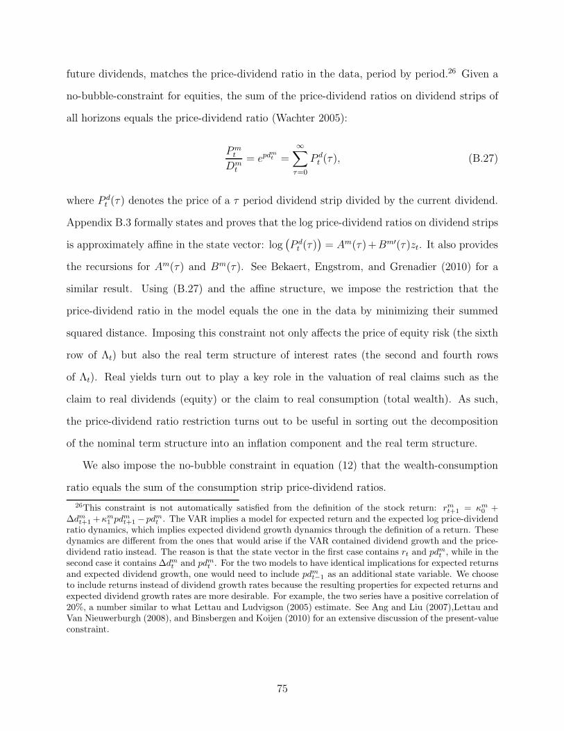
future dividends, matches the price-dividend ratio in the data, period by period.26 Given a
no-bubble-constraint for equities, the sum of the price-dividend ratios on dividend strips of
all horizons equals the price-dividend ratio (Wachter 2005):
Pmt
Dmt
= epdmt =
∞∑
τ=0
P dt (τ), (B.27)
where P dt (τ) denotes the price of a τ period dividend strip divided by the current dividend.
Appendix B.3 formally states and proves that the log price-dividend ratios on dividend strips
is approximately affine in the state vector: log(P dt (τ)
)= Am(τ)+Bm′(τ)zt. It also provides
the recursions for Am(τ) and Bm(τ). See Bekaert, Engstrom, and Grenadier (2010) for a
similar result. Using (B.27) and the affine structure, we impose the restriction that the
price-dividend ratio in the model equals the one in the data by minimizing their summed
squared distance. Imposing this constraint not only affects the price of equity risk (the sixth
row of Λt) but also the real term structure of interest rates (the second and fourth rows
of Λt). Real yields turn out to play a key role in the valuation of real claims such as the
claim to real dividends (equity) or the claim to real consumption (total wealth). As such,
the price-dividend ratio restriction turns out to be useful in sorting out the decomposition
of the nominal term structure into an inflation component and the real term structure.
We also impose the no-bubble constraint in equation (12) that the wealth-consumption
ratio equals the sum of the consumption strip price-dividend ratios.
26This constraint is not automatically satisfied from the definition of the stock return: rmt+1 = κm
0 +∆dmt+1 +κm
1 pdmt+1 − pdmt . The VAR implies a model for expected return and the expected log price-dividendratio dynamics, which implies expected dividend growth dynamics through the definition of a return. Thesedynamics are different from the ones that would arise if the VAR contained dividend growth and the price-dividend ratio instead. The reason is that the state vector in the first case contains rt and pdm
t, while in the
second case it contains ∆dmt
and pdmt. For the two models to have identical implications for expected returns
and expected dividend growth, one would need to include pdmt−1 as an additional state variable. We chooseto include returns instead of dividend growth rates because the resulting properties for expected returns andexpected dividend growth rates are more desirable. For example, the two series have a positive correlation of20%, a number similar to what Lettau and Ludvigson (2005) estimate. See Ang and Liu (2007),Lettau andVan Nieuwerburgh (2008), and Binsbergen and Koijen (2010) for an extensive discussion of the present-valueconstraint.
75

Human Wealth Share We define the labor income share, list, as the ratio of aggregate
labor income to aggregate consumption. It is 0.826 on average in our sample. The human
wealth share is the ratio of human wealth to total wealth; it is a function of the labor income
share and the price-dividend ratios on human and total wealth: hwst = listepd
lt−1
ewct−1. We
impose on the estimation that hwst lies between 0 and 1 at each time t. At the optimum,
this constraint is satisfied.27
B.8 Point estimates
Below, we report the point estimates for the VAR companion matrix Ψ, the Cholesky de-
composition of the covariance matrix Σ.5 (multiplied by 100), and the market price of risk
parameters Λ0 and Λ1 for our benchmark specification. We recall that the market price of risk
parameter matrix Λ1 pre-multiplies the state zt, which has a (non-standardized) covariance
matrix Ω.
Ψ =
0.5429 0.7650 -0.3922 0.9475 0 0 0 0 0 0
-0.0605 0.9893 0.0751 0.4266 0 0 0 0 0 0
-0.0519 0.1669 0.7020 0.1496 0 0 0 0 0 0
0.0734 -0.0752 0.0094 0.4123 0 0 0 0 0 0
0.4109 -0.2856 -2.3795 -3.0151 0.9345 -0.0003 0 0 0 0
0.1036 0.3773 -2.0304 0.9121 -0.0434 0.0992 0 0 0 0
0.0006 0.4722 -1.1454 -0.1641 -0.0086 0.0728 0 0 0 0
0.2124 0.2100 -0.5441 -0.5424 0.0030 0.1258 0 0 0 0
-0.0048 0.1020 -0.0414 0.3583 0.0029 -0.0006 -0.0044 0.0071 0.3708 0
0.0456 -0.0441 -0.0940 -0.1228 0.0032 -0.0063 0.0322 -0.0162 0.5856 -0.1223
27We impose that aggregate labor income grows at the same rate as aggregate consumption (µl = µc).We rescale the level of consumption to end up with the same average labor income share (after imposingµl = µc) as in the data (before rescaling).
76
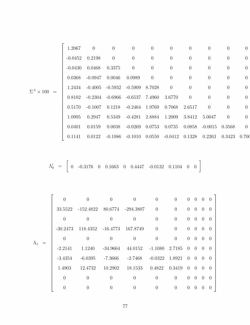
Σ.5 × 100 =
1.2067 0 0 0 0 0 0 0 0 0
-0.0452 0.2198 0 0 0 0 0 0 0 0
-0.0430 0.0468 0.3375 0 0 0 0 0 0 0
0.0368 -0.0947 0.0046 0.0989 0 0 0 0 0 0
1.2434 -0.4005 -0.5932 -0.5909 8.7028 0 0 0 0 0
0.8102 -0.2304 -0.6966 -0.6537 7.4960 3.6770 0 0 0 0
0.5170 -0.1007 0.1218 -0.2464 1.9769 0.7068 2.6517 0 0 0
1.0995 0.2947 0.5349 -0.4281 2.8884 1.2009 3.8412 5.0047 0 0
0.0401 0.0159 0.0038 -0.0269 0.0753 0.0735 0.0858 -0.0015 0.3568 0
0.1141 0.0122 -0.1086 -0.1010 0.0550 -0.0412 0.1328 0.2263 0.3423 0.7007
Λ′0 =
[0 -0.3176 0 0.1663 0 0.4447 -0.0132 0.1104 0 0
]
Λ1 =
0 0 0 0 0 0 0 0 0 0
33.5522 -152.4822 80.6774 -294.3807 0 0 0 0 0 0
0 0 0 0 0 0 0 0 0 0
-30.2473 118.4352 -16.4773 167.8749 0 0 0 0 0 0
0 0 0 0 0 0 0 0 0 0
-2.2141 1.1240 -34.9664 44.0152 -1.1080 2.7185 0 0 0 0
-3.4354 -6.0395 -7.3666 -2.7468 -0.0322 1.8921 0 0 0 0
1.4903 12.4732 10.2902 18.1533 0.4822 0.3419 0 0 0 0
0 0 0 0 0 0 0 0 0 0
0 0 0 0 0 0 0 0 0 0
77

We compute OLS standard errors for the elements of Ψ and report the coefficients with
a t-stat greater than 1.98 in bold. Bootstrap standard errors on the market price of risk
parameters are available upon request. They are derived as part of the method explained in
Appendix B.9.
The implied point estimates for Ac1 are given by:
Ac1 =
-0.5191
-25.8220
1.8370
-26.0851
0.0854
-0.0067
-0.0070
0.0113
0.5866
0
while the implied point estimate for the constant is Ac0 = 5.8082.
B.9 Bootstrap standard errors
We obtain standard errors on the moments of the estimated wealth-consumption ratio by
bootstrap. More precisely, we conduct two bootstrap exercises leading to two sets of standard
errors. In each exercise, we draw with replacement from the VAR innovations εt. We draw
row-by-row in order to preserve the cross-correlation structure between the state innovations
(Step 1). Given the point estimates for Ψ and Σ as well as the mean vector µ, we recursively
reconstruct the state vector (Step 2). We then re-estimate the mean vector, companion
matrix, and innovation covariance matrix (Step 3). With the new state vector and the new
VAR parameters in hand, we re-estimate the market price of risk parameters in Λ0 and
78
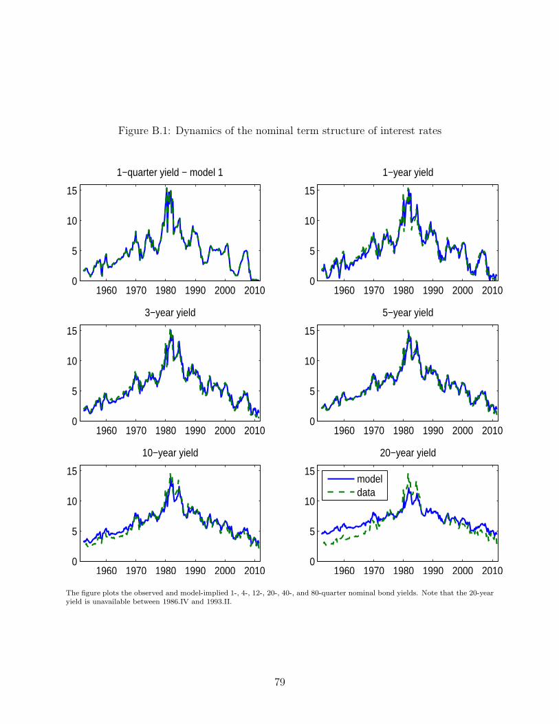
Figure B.1: Dynamics of the nominal term structure of interest rates
1960 1970 1980 1990 2000 20100
5
10
15
1−quarter yield − model 1
1960 1970 1980 1990 2000 20100
5
10
15
1−year yield
1960 1970 1980 1990 2000 20100
5
10
15
3−year yield
1960 1970 1980 1990 2000 20100
5
10
15
5−year yield
1960 1970 1980 1990 2000 20100
5
10
15
10−year yield
1960 1970 1980 1990 2000 20100
5
10
15
20−year yield
modeldata
The figure plots the observed and model-implied 1-, 4-, 12-, 20-, 40-, and 80-quarter nominal bond yields. Note that the 20-yearyield is unavailable between 1986.IV and 1993.II.
79

Figure B.2: Nominal bond risk premia
1940 1960 1980 2000 2020−2
−1
0
1
2
3
4
5
Perce
nt per y
ear
5−yr Risk Premium on 5−yr Nominal Bond
modeldata
1940 1960 1980 2000 2020−8
−6
−4
−2
0
2
4
6
8
Perce
nt per y
ear
Cochrane−Piazzesi factor
modeldata
The left panel plots the 5-year nominal bond risk premium on a 5-year nominal bond in model and data. It is defined as thedifference between the nominal 5-year yield and the expected future 1-quarter yield averaged over the next 5 years. It representsthe return on a strategy that buys and holds a 5-year bond until maturity and finances this purchase by rolling over a 1-quarterbond for 5 years. The right panel plots the Cochrane-Piazzesi factor in model and data. It is a linear combination of theone-year nominal yield and 2- through 5-year forward rates. This linear combination is a good predictor of the one-quarterbond risk premium.
Λ1 (Step 4). Just as in the main estimation, we use 2,500 quarters to approximate the
infinite-horizon sums in the strip price-dividend ratio calculations. We limit the estimation
in Step 4 to 500 function evaluations for computational reasons. In some of the bootstrap
iterations, the optimization in Step 4 does not find a feasible solution. This happens, for
example when no parameter choices keep the human wealth share less than 100% or the
consumption or labor income claim finite. We discard these bootstrap iterations. These new
market price of risk parameters deliver a new wealth-consumption ratio time series (Step 5).
With the bootstrap time series for consumption growth and the wealth-consumption ratio,
we can form all the moments in Table 2. We repeat this procedure 1,000 times and report
the standard deviation across the bootstrap iterations. We conduct two variations on the
above algorithm. Each bootstrap exercise takes about 12 hours to compute on an 8-processor
computer. The more conservative standard errors from the second bootstrap exercise are
the ones reported in Table 2.
In the first exercise, we only consider sampling uncertainty in the last four elements
80
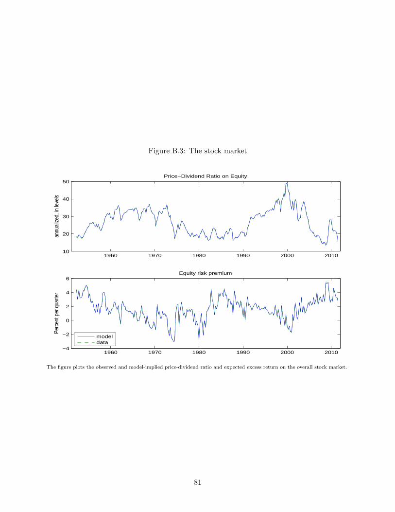
Figure B.3: The stock market
1960 1970 1980 1990 2000 201010
20
30
40
50Price−Dividend Ratio on Equity
annu
alize
d, in
leve
ls
1960 1970 1980 1990 2000 2010−4
−2
0
2
4
6
Perc
ent p
er q
uarte
r
Equity risk premium
modeldata
The figure plots the observed and model-implied price-dividend ratio and expected excess return on the overall stock market.
81

Figure B.4: Decomposing the 5-year nominal yield
1940 1960 1980 2000 2020−2
0
2
4
6
8
10
12
14
16
Percen
t per ye
ar
Decomposing Nominal Yield on 5−Year Bond
ynomyrealexp inflIRP
0 50 100 150−0.5
0
0.5
1
1.5
2
2.5Term structure of nominal bond risk premia
quarters
Percen
t per ye
ar
nominalrealinflation
The left panel decomposes the 5-year yield into the real 5-year yield, expected inflation over the next 5-years, and the inflationrisk premium. The right panel decomposes the average nominal bond risk premium into the average real rate risk premium andinflation risk premium for maturities ranging from 1 to 120 quarters. The nominal (real) bond risk premium at maturity τ isdefined as the nominal (real) τ -quarter yield minus the average expected future nominal (real) 1-quarter yield over the next τquarters. The τ -quarter inflation risk premium, labeled as IRP, is the difference between the τ -quarter nominal and real riskpremia.
Figure B.5: Decomposing the yield on a consumption strip
0 100 200 300 400 500 600 700 800 900 1000−1
−0.5
0
0.5
1
1.5Decomposing consumption strip yields
Perce
nt pe
r yea
r
maturity in quarters
cons strip yieldreal bond yield − mu
c
yccr
The figure decomposes the yield on a consumption strip of maturity τ , which goes from 1 to 1,000 quarters, into a real bondyield minus deterministic consumption growth on the one hand and the yield on a security that only carries the consumptioncash flow risk on the other hand. See B.4 for a detailed discussion of this decomposition.
82
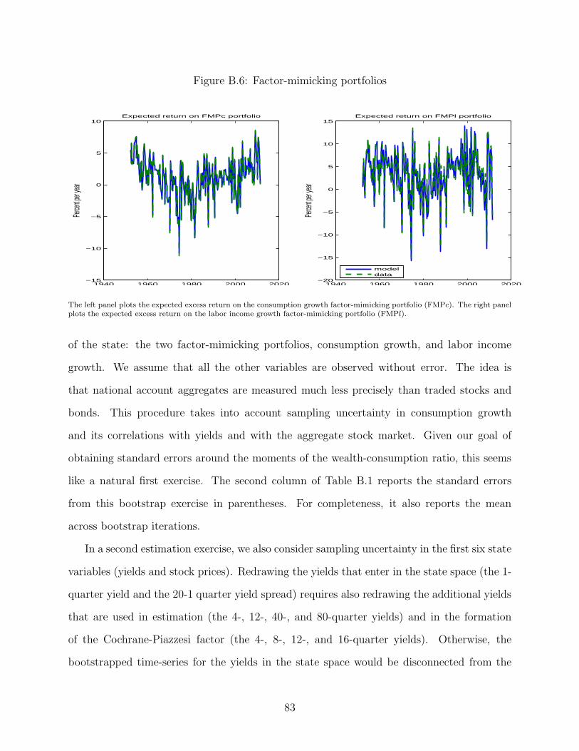
Figure B.6: Factor-mimicking portfolios
1940 1960 1980 2000 2020−15
−10
−5
0
5
10
Perce
nt per y
ear
Expected return on FMPc portfolio
1940 1960 1980 2000 2020−20
−15
−10
−5
0
5
10
15
Perce
nt per y
ear
Expected return on FMPl portfolio
modeldata
The left panel plots the expected excess return on the consumption growth factor-mimicking portfolio (FMPc). The right panelplots the expected excess return on the labor income growth factor-mimicking portfolio (FMPl).
of the state: the two factor-mimicking portfolios, consumption growth, and labor income
growth. We assume that all the other variables are observed without error. The idea is
that national account aggregates are measured much less precisely than traded stocks and
bonds. This procedure takes into account sampling uncertainty in consumption growth
and its correlations with yields and with the aggregate stock market. Given our goal of
obtaining standard errors around the moments of the wealth-consumption ratio, this seems
like a natural first exercise. The second column of Table B.1 reports the standard errors
from this bootstrap exercise in parentheses. For completeness, it also reports the mean
across bootstrap iterations.
In a second estimation exercise, we also consider sampling uncertainty in the first six state
variables (yields and stock prices). Redrawing the yields that enter in the state space (the 1-
quarter yield and the 20-1 quarter yield spread) requires also redrawing the additional yields
that are used in estimation (the 4-, 12-, 40-, and 80-quarter yields) and in the formation
of the Cochrane-Piazzesi factor (the 4-, 8-, 12-, and 16-quarter yields). Otherwise, the
bootstrapped time-series for the yields in the state space would be disconnected from the
83
other yields. For this second exercise, we augment the VAR with the following yield spreads:
4-20, 8-20, 12-20, 16-20, 40-20, and 80-20 quarter yield spreads. We let these spreads depend
on their own lag and on the lagged 1-quarter yield. Additional dependence on the lagged 20-1
quarter yield makes little difference. In Step 1, we draw from the yield spreads-augmented
VAR innovations. This allows us to take into account the cross-dependencies between all
the yields in the yield curve. In addition to recursively rebuilding the state variables in
Step 2, we also rebuild the six yield spreads. With the bootstrapped yields, we reconstruct
the forward rates, 1-year excess bond returns, re-estimate the excess bond return regression,
and re-construct the Cochrane-Piazzesi factor. Steps 3 through 5 are the same as in the
first exercise. One additional complication arises because the bootstrapped yields often turn
negative for one or more periods. Since negative nominal yields never happen in the data
and make no economic sense, we discard these bootstrap iterations. We redraw from the
VAR innovations until we have 1,000 bootstrap samples with strictly positive yields at all
maturities. This is akin to a rejection-sampling procedure. One drawback is that there is
an upward bias in the yield curve. The average 1-quarter yield is 0.8% per annum higher
in the bootstrap sample than in the data. This translates in a small downward bias in the
average wealth consumption ratio: the average log wealth-consumption ratio is 0.17 lower
in the bootstrap than in the data. The third column of Table B.1 reports the standard
errors from this bootstrap exercise in parentheses. As expected, the standard errors from
the second bootstrap exercise are somewhat bigger. However, their difference is small.
84

Table B.1: Bootstrap standard errors
This table displays bootstrap standard errors on the unconditional moments of the log wealth-consumption ratio wc, its firstdifference ∆wc, and the log total wealth return rc. The last but one row reports the time-series average of the conditionalconsumption risk premium, E[Et[r
c,et ]], where rc,e denotes the expected log return on total wealth in excess of the risk-free
rate and corrected for a Jensen term. The second and third columns report the results from two bootstrap exercises, describedabove. The table reports the mean and standard deviation (in parentheses) across 1,000 bootstrap iterations.
Moments Bootstrap 1 Bootstrap 2
Std[wc] 16.26% 15.24%
(3.39) (4.30)
AC(1)[wc] 0.95 0.93
(0.00) (0.03)
AC(4)[wc] 0.83 0.74
(0.01) (0.08)
Std[∆wc] 4.86% 5.07%
(0.98) (1.16)
Std[∆c] 0.44% 0.44%
(0.03) (0.03)
Corr[∆c,∆wc] .02 .12
(0.06) 0.06)
Std[rc] 4.90% 5.16%
(2.21) (1.16)
Corr[rc,∆c] .12 .21
(0.07) (0.07)
E[Et[rc,et ]] .46% 0.53%
(0.11) (0.16)
E[wc] 6.29 5.69
(0.48) (0.49)
2006 Wealth (in millions) 2.65 2.52
(0.32) (0.27)
hws 0.86 0.86
boot std (0.03) (0.03)
85

Online Appendix for “The Wealth-Consumption Ratio”
NOT FOR PUBLICATION
C Appendix: Robustness
The results of our estimation exercise are robust to different specifications of the state vector
z and restrictions on the benchmark law of motion for the state z. We compare ten models
to gain insight into what part of the model structure drives which result.
Model 1 is the benchmark model from the paper. It has the ten elements in the VAR
and the companion matrix Ψ, as specified in equation (1) of the paper. Models 2 through 6
simplify the benchmark model, starting from two minimal models, and gradually building up
to the benchmark model. Models 7 through 10 have the same state space as the benchmark
Model 1, but simplify the dynamics of the state space, i.e., Ψ. These variations are selected
to give insight into what drives our main result, as well as to verify the robustness of our
results.
Table C.1 summarizes the goodness-of-fit of all ten models; each column refers to a
model. The first ten rows report the root mean-squared pricing errors (RMSE) on ten key
asset pricing moments the model is trying to fit. We estimate the market price of risk by
minimizing a function of these RMSEs. The last four rows express the goodness fit of the
models, as well as a log difference with the benchmark model. The first comparison is based
on the simple average RMSE (labeled SM). The second comparison is based on a weighted
average RMSE (labeled WM), where the weights reflect the importance of each moment in
the optimization routine. It shows that the benchmark Model 1 has the best fit of all the
models we consider, justifying its label.
We now turn to a detailed discussion of these models and what they teach us about the
wealth-consumption ratio.
1

C.1 Simpler models
C.1.1 Model 2
The simplest model we consider, Model 2, only contains the short rate (nominal 1-quarter
bond yield), inflation, the yield spread (20-quarter minus 1-quarter yield), consumption
growth, and labor income growth (in that order). It strips out from the state the CP factor,
the PD ratio on the stock market, the excess return on the stock market, and the factor-
mimicking portfolios for consumption growth and labor income growth (computed from the
cross-section of stocks). Model 2 is the most basic model that still allows us to price the
claims to aggregate consumption and labor income. Inflation is necessary to go from nominal
to real pricing kernels and yields. The term structure with two maturities in the state vector
is quite basic. The model purposely ignores all equity moments.
Consistent with the logic explained in the estimation section of the paper, we estimate
two elements in the constant market price of risk vector Λ0 and the two corresponding rows
(of three elements each) in the matrix Λ1, which governs the time variation in prices of risk.
These are the first and third elements corresponding to the short rate and the yield spread.
This is the minimal structure needed to provide a reasonably good fit to the term structure
of interest rates. The model also does a surprisingly good job at matching the dynamics of
the 5-year nominal bond risk premium and a decent job at matching the dynamics of the CP
factor. Because the CP factor, a linear combination of 1- through 5-year yields, is not in the
state, the model implicitly puts less weight on matching that part of the term structure and
instead pays more attention to matching the long end of the yield curve. This results in a
lower estimate for the 20-year nominal yields than in Model 1 (6.74% in Model 2 vs. 6.85%
in Model 1), bringing it closer to the data (6.23%). The model-implied 20-year real yield is
correspondingly lower (2.49% in Model 2 vs. 2.87% in Model 1). Similarly, the annualized
risk premium (average excess return over a 1-period bond yield) on a (hypothetical) 50-year
real bond is 1.29% in Model 2 vs. 1.84% in Model 1.
2

Model 2 clearly illustrates our main conclusion: that the real term structure of interest
rates is the key determinant of the wealth-consumption ratio. The lower long-term real
yields in Model 2 translate into a higher mean wealth-consumption ratio : 113 versus 83
in Model 1. The average consumption risk premium, the excess return on the claim to
aggregate consumption, is 2.11% in Model 2 versus 2.38% in Model 1. While the mean
levels differ, the dynamics of the WC ratio in Model 2 are nearly identical to that in Model
1: their correlation is 99.03% and the volatilities are nearly identical (18.9% versus 18.6%).
The correlation between the consumption risk premia in the two model is 97.6%. The main
reason for the similar dynamics in wealth-consumption ratios and consumption risk premia
is that long-term real yields comove strongly: the 20-year real yields have a time series
correlation of 99.86%.
Offsetting the strong real yield correlation is the fact that the cash flow risk in the
consumption claim (as opposed to the real rate risk) is priced somewhat differently in Model
2 than in Model 1. Because the state vectors differ, expected consumption growth dynamics
differ for Models 1 to 6. And innovations to future consumption growth are priced differently
across models. For example, the yield on a claim to the risky part of aggregate consumption
50 years from now is about zero in Model 1. This implies that the entire yield on the 50-
year consumption strip (trend growth plus risky fluctuations around that trend) equals the
yield on a 50-year coupon bond (with cash flow adjusted for trend consumption growth).
In contrast, the risky 50-year consumption strip has a yield that is 20 basis points above
that on the corresponding real bond in Model 2, implying substantially more cash-flow
risk. The reason for this difference is that real bond yields and yields on the risky part of
the consumption strip are strongly negatively correlated in Model 1 and strongly positively
correlated in Model 2. Hence, the cash flow risk of the consumption claim actually hedges the
real rate risk in Model 1 while the exposures go in the same direction in Model 2. The extra
consumption cash flow risk in Model 2 translates in a higher consumption risk premium,
ceteris paribus. These differences in consumption cash flow risk show up clearly in the form
3

of higher costs of consumption fluctuations in Model 2. However, the much lower bond risk
premium more than offsets the higher consumption cash flow risk so that the consumption
risk premium still ends up lower than in the benchmark Model 1.
In summary, Model 2 is simple and generates results that are qualitatively and quanti-
tatively similar to our benchmark results. But, by construction, Model 2 does an awful job
at pricing the stock-based moments. This immediately raises the question of whether the
low consumption risk premium and high wealth-consumption ratio are the result of ignoring
important sources of risk when pricing the consumption claim. To dispel this possibility, we
consider both bond- and stock-based moments in our benchmark model.
C.1.2 Model 3
To understand the role of equity-based moments better, we propose Model 3, which focusses
on fitting the equity return and the price-dividend ratio on the stock market while ignoring
the bond-based moments. The state vector contains the short rate, inflation, the PD ratio
on the stock market, the excess return on the stock market, consumption growth, and labor
income growth (in that order). It strips out from the state the CP factor, the yield spread,
and the factor-mimicking portfolios for consumption growth and labor income growth. This
is the minimal model that enables us to fit the aggregate stock market facts.
We estimate two elements in Λ0 and six elements in Λ1, associated with the short rate
and the excess return on equity (2 in row 1 and 4 in the equity row, consistent with the
structure of full model). Because it implies a one-factor structure for the nominal yield curve,
it does substantially worse than Models 1 and 2 in fitting the term structure of yields of all
maturities, as well as the CP factor; see Table C.1. The model implies an annual 20-year real
yield of 2.66%, a 50-year real bond risk premium of 1.50%, a consumption risk premium of
2.24%, and a mean wealth-consumption ratio of 96. These numbers are in between those of
Model 1 and Model 2. Hence, a model that is substantially less rich on the term structure side
but fits the equity excess return and price-dividend series very well generates qualitatively
4

similar conclusions, at least with respect to the mean wealth-consumption ratio and the
associated consumption risk premium.
The dynamics of the wealth-consumption ratio do differ somewhat from those of the
benchmark model. The volatility of the WC ratio is lower at 14% and the time series
correlation with the WC ratio of Model 1 is 93.0%, which is the lowest among all alternative
models we consider. There are episodes in the sample where this results in the WC ratio of
Model 3 going up when the WC ratio of all other models goes down. The reason for the gap
is that, while the long-term real yield is still highly correlated with that in Model 1 (91.7%),
the consumption risk premium is much less so (67.1%). The low correlation between the
consumption risk premium in Models 2 and 3 (68.8%) shows that emphasizing the pricing
of risk in the stock market at the expense of the risk pricing in the bond market makes a
tangible difference. In particular, Model 3 fails completely at capturing the dynamics of the
nominal bond risk premium as described by the CP factor. This has implications for the
cost of consumption fluctuations.
C.1.3 Model 4
Model 4 combines Models 2 and 3. The state vector contains the short rate, inflation, the
yield spread, the PD ratio, the excess return on the stock market, consumption growth, and
labor income growth (in that order). It leaves out the CP factor and the factor-mimicking
portfolios for consumption growth and labor income growth. Model 4 adds a second term
structure factor to Model 3. Alternatively, it adds the aggregate stock market moments to
Model 2. Model 4 generates small bond pricing and stock pricing errors, but to sizeable
pricing errors on CP and the factor-mimicking portfolio returns. Naturally, model 4 fits
better than either Models 2 or 3, but the log difference in simple (weighted) average pricing
errors is still 62% (54%) with the benchmark Model 1. See Table C.1. In terms of the
long-term real yield and bond risk premia, Model 4 is very close to Model 2. In terms of the
consumption risk premium, it is close to Model 3. The mean wealth-consumption ratio is 96
5

in Model 4, similar to the 83 average in Model 1. The wealth-consumption ratios in Models
1 and 4 have a correlation of 99.85%.
Like Model 3, Model 4 implies a positive correlation between real bond prices and the
prices on the consumption strip with only cash flow risk; in Model 4 that correlation is higher
still. This results in a substantial risk premium for the consumption strip of about 30 bps at
50-year horizon. The mean cost of consumption fluctuations is 52.9% for Model 4 (compared
to 36.2% for Model 2 and 16.2% for Model 3).
C.1.4 Model 5
In Model 5, we add back the CP factor to the state vector of Model 4. This is the full model,
except without the two factor-mimicking portfolio returns in the state. This model results
in a substantially better fit for the CP factor. In order to fit the CP factor better, the model
focuses more on the 1- to 5-year bond yields and less on the long end of the term structure.
The result is higher model-implied nominal and real long-term bond yields. The 20-year
nominal (real) yield is 7.01% (2.99%), the highest among all models. The 50-year real bond
risk premium is 2.05% per year. The mean wealth-consumption ratio is 69 compared to 96
in Model 4 (and 83 in Model 1). The wealth-consumption ratios in Models 1 and 5 have a
correlation of 99.97%.
Going from Model 4 to Model 5, there is a dramatic change in the consumption cash flow
risk. In Model 5, the prices of strips that pay the risky part of aggregate consumption and
the prices of real bonds are strongly negatively correlated, so that the cash flow part of the
consumption strip hedges the real rate risk in these strips. This lowers the risk premium and
the overall yield on the consumption claim. It is the low consumption cash flow risk that
is responsible for the lower cost of consumption fluctuations in Model 5 (-1.8%), relative
to Model 4 (52.9%). The higher consumption risk premium of 2.67% is therefore solely
attributable to the higher real yields and bond risk premia, not to higher consumption cash
flow risk.
6

C.1.5 Model 6
In Model 6, we add back the two factor-mimicking portfolios in the state but leave out the CP
factor. Naturally, this results in a substantially better fit for the factor-mimicking portfolios
at the expense of the fit for the CP factor. The bond pricing is similar to that in Models 2
and 4 with relatively low long-term rates and real bond risk premia, a low consumption risk
premium, and a high mean wealth-consumption ratio (115). The factor-mimicking portfolios
add priced sources of equity risk, which add to the riskiness of the consumption claim. Adding
the factor-mimicking portfolios (going from Model 4 to Model 6) substantially increases the
mean cost of consumption fluctuations from 52.9% in Model 4 to 68.1% in Model 6. Despite
the additional consumption cash flow risk, the overall consumption risk premium is lower in
Model 6 than in Model 4 because the real bond risk premium is lower.
C.1.6 Summary
Figure C.1 shows the wealth-consumption ratio for the benchmark Model 1 and the five sim-
pler (and sequentially more complex) models. They show that the wealth-consumption ratios
are highly correlated across models, with all numbers lying between 91.23% and 99.98%. If
we exclude Model 3, the correlation is never below 98%. The high comovement is largely
driven by the high comovement in the real yield curve across models. For example, the real
20-year yield across all six models varies between 91.68% and 99.97%. Again, the lowest cor-
relation comes from Model 3; all other models have real yield correlations in excess of 99%.
Since all models price the short-term bond perfectly, and because one factor accounts for a
lot of the comovement across bonds of various maturities, that conclusion is not surprising.
The main difference between models, therefore, is in the level rather than the dynamics
of the wealth-consumption ratio. The average varies from 69 in Model 5 to 115 in Model
6. As discussed above, this difference is largely accounted for by differences in the mean
(real) yield curve, which is plotted in Figure C.2. The long-term real yield is highest in
Models 1 and 5, the only two that contain the CP factor. Including the CP factor forces the
7
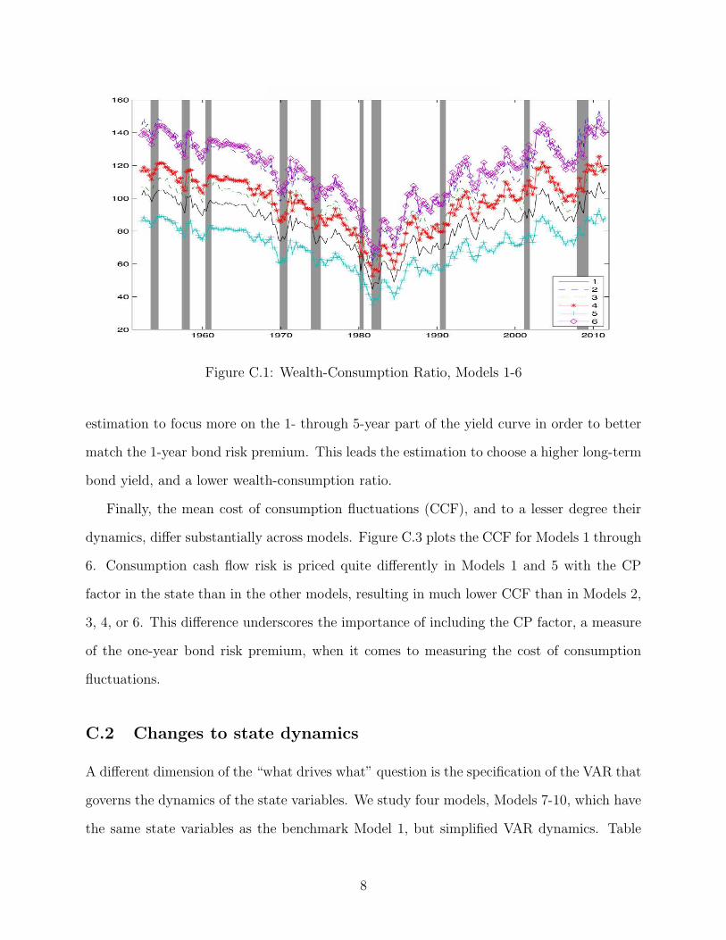
Figure C.1: Wealth-Consumption Ratio, Models 1-6
estimation to focus more on the 1- through 5-year part of the yield curve in order to better
match the 1-year bond risk premium. This leads the estimation to choose a higher long-term
bond yield, and a lower wealth-consumption ratio.
Finally, the mean cost of consumption fluctuations (CCF), and to a lesser degree their
dynamics, differ substantially across models. Figure C.3 plots the CCF for Models 1 through
6. Consumption cash flow risk is priced quite differently in Models 1 and 5 with the CP
factor in the state than in the other models, resulting in much lower CCF than in Models 2,
3, 4, or 6. This difference underscores the importance of including the CP factor, a measure
of the one-year bond risk premium, when it comes to measuring the cost of consumption
fluctuations.
C.2 Changes to state dynamics
A different dimension of the “what drives what” question is the specification of the VAR that
governs the dynamics of the state variables. We study four models, Models 7-10, which have
the same state variables as the benchmark Model 1, but simplified VAR dynamics. Table
8

Figure C.2: Average Yield Curve, Models 1-6
Figure C.3: Cost of Consumption Fluctuations, Models 1-6
9
C.1 lists the asset pricing errors of these models in its four last columns.
C.2.1 Model 7
In Model 7, we zero out all non-significant elements of the Ψ matrix. This leads to only two
zeros in the 4× 4 bond block. However, the pd ratio only loads on its own lag, and expected
stock returns are only significantly predicted by the lagged pd ratio. The factor-mimicking
portfolio returns depend on the lagged excess stock return, and the FMP for consumption
growth additionally on lagged inflation. The consumption growth rate is predicted signifi-
cantly by the yield spread, the pd ratio, and its own lag. Labor income growth is predicted
only by lagged consumption growth. After imposing these zero restrictions, we re-estimate
the constrained companion matrix.
Despite the substantial changes to the state vector’s dynamics, we find similar results.
The wealth-consumption ratio in Model 7 has a correlation of 99.98% with that in Model
1. The model-implied 20-year real yields are essentially perfectly correlated because the
dynamics of the bond block did not change much. The average long-term real yield and real
bond risk premium are higher, though, which results in a lower mean wealth-consumption
ratio (67 in Model 7 vs. 83 in Model 1) and a higher consumption risk premium (2.74%
vs. 2.38%). Some of the increase in the consumption risk premium is due to a higher
reward for consumption cash flow risk. The reason is that the prices of risky consumption
cash flow strips are less negatively correlated with real bond prices than in the benchmark
model. The higher consumption cash flow risk leads to a cost of consumption fluctuations
that is slightly higher on average (4.0% compared to -2.4% in Model 1). While expected
consumption growth in Model 7 still has a high correlation of 96.3% with that in Model 1,
that small difference is sufficient to lead to noticeable differences in the consumption cash
flow risk premium and the cost of consumption fluctuations.
10

C.2.2 Models 8 and 9
In Model 8, we only zero out only the elements in the pd and stock return equation that are
not significant. In Model 9, we zero out only the elements in the factor-mimicking portfolio
return equations that are not significant. In both cases, this leads to very minor changes
to the benchmark results because the term structure implications of Models 1, 8, and 9 are
nearly identical and the expected consumption growth dynamics are identical.
C.2.3 Model 10
In Model 10, we only zero out the elements in the consumption and labor income growth
equations that are not significant. This model is similar to Model 7, which clarifies that the
change in results between Model 1 and 7 is largely due to the changed consumption and
labor income growth dynamics. In Model 10, we have the lowest mean wealth-consumption
ratio among all models, at 62, and the highest consumption risk premium at 2.94% per year.
The cost of consumption fluctuations is 9.9% on average.
C.2.4 Summary
Figure C.4 shows the wealth-consumption ratio for the benchmark Model 1 and the four
simpler models in terms of VAR dynamics, Models 7-10. They show that the wealth-
consumption ratios are highly correlated across models, with all numbers lying between
99.62% and 99.99%. The high comovement is largely driven by the high comovement in
the real yield curve across models and the high correlation in expected consumption growth
dynamics. For example, the real 20-year yield across the five models is nearly perfect.
The main difference between models, therefore, is in the level rather than the dynamics
of the wealth-consumption ratio. The average varies from 62 in Model 10 to 87 in Model
9. As discussed above, this small difference is largely accounted for by small differences in
the mean (real) yield curve, which is plotted in Figure C.5. Despite these differences, the
mean wealth-consumption ratios of all 10 models (ranging from 62 to 115) are all more than
11

Figure C.4: Wealth-Consumption ratio Models 1 and 7-10
double the mean price-dividend ratio on stocks, which is 26 in our sample.
The range across all 10 models for the consumption risk premium is between 52 bps
and 74 bps per quarter or between 2.07% for Model 6 and 2.94% for Model 10 per year. It
deserves emphasis that even the highest value, implies a consumption risk premium less than
half as big as the mean equity risk premium of 6.4%. Also, the narrow range of estimates
(87 basis points per year) is testimony to the robustness of our results.
Figure C.6 shows that the cost of consumption fluctuations is much less affected by
zeroing out elements of the VAR dynamics, compared to changing the elements in the state
vector itself.
C.3 Changing bond market dynamics
In a last robustness exercise, we relax the block-diagonal nature of the Ψ matrix and allow
the bond market dynamics in the first four equations of the VAR to depend on the lagged
stock market variables (next four elements). Based on a first-stage equation-by-equation
12
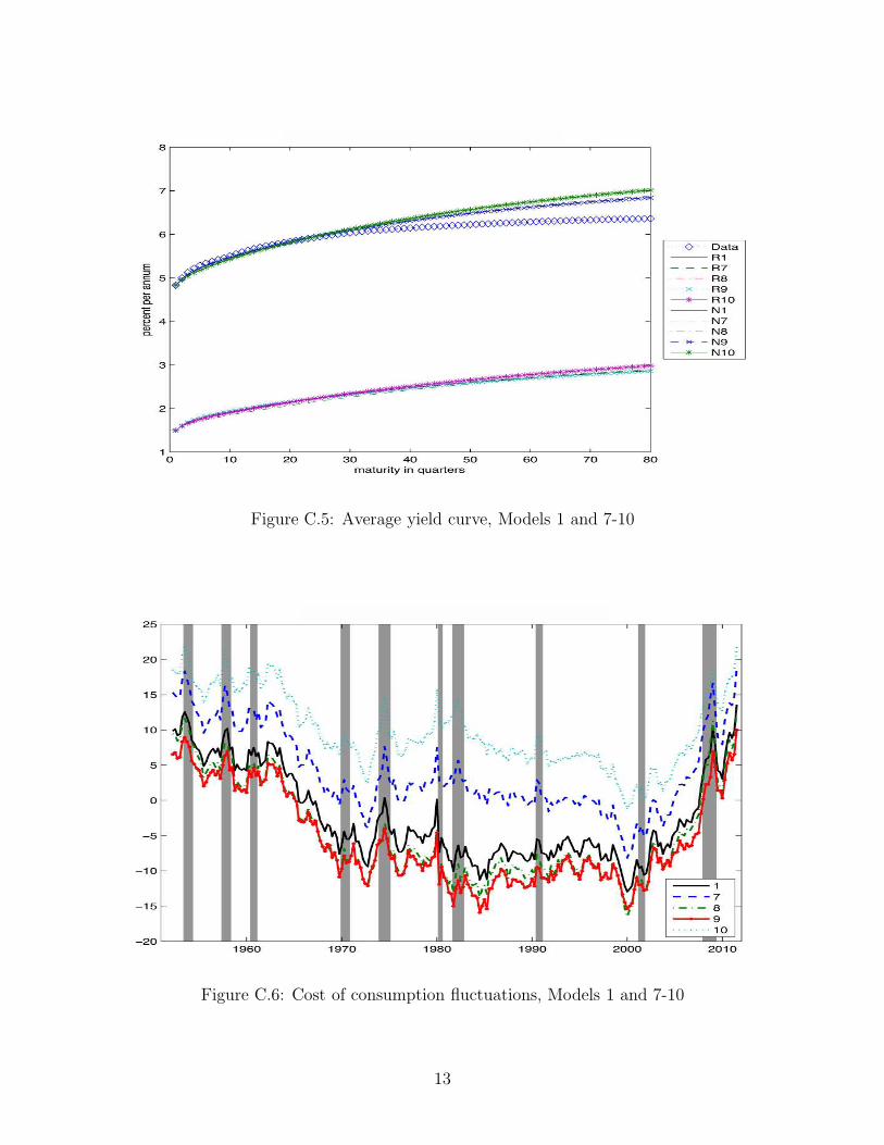
Figure C.5: Average yield curve, Models 1 and 7-10
Figure C.6: Cost of consumption fluctuations, Models 1 and 7-10
13
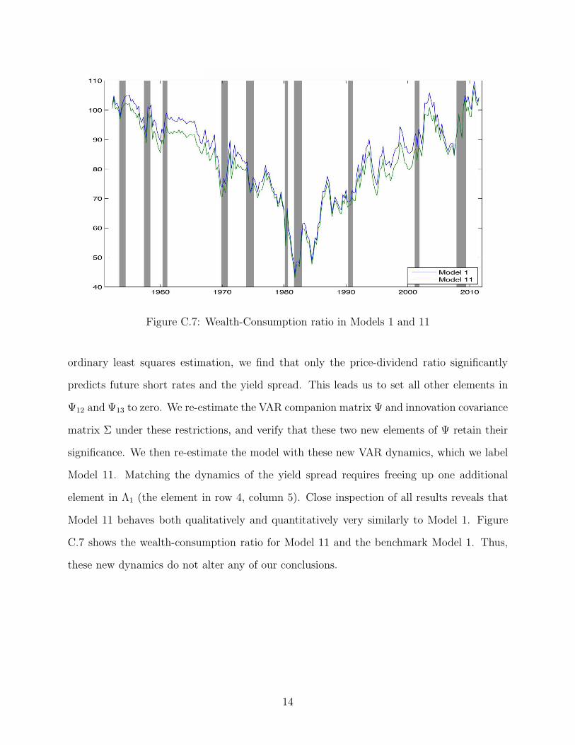
Figure C.7: Wealth-Consumption ratio in Models 1 and 11
ordinary least squares estimation, we find that only the price-dividend ratio significantly
predicts future short rates and the yield spread. This leads us to set all other elements in
Ψ12 and Ψ13 to zero. We re-estimate the VAR companion matrix Ψ and innovation covariance
matrix Σ under these restrictions, and verify that these two new elements of Ψ retain their
significance. We then re-estimate the model with these new VAR dynamics, which we label
Model 11. Matching the dynamics of the yield spread requires freeing up one additional
element in Λ1 (the element in row 4, column 5). Close inspection of all results reveals that
Model 11 behaves both qualitatively and quantitatively very similarly to Model 1. Figure
C.7 shows the wealth-consumption ratio for Model 11 and the benchmark Model 1. Thus,
these new dynamics do not alter any of our conclusions.
14
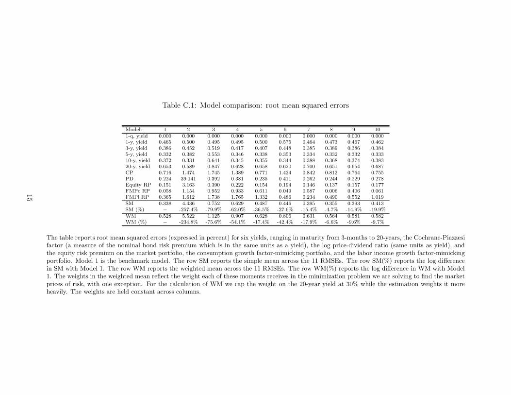
Table C.1: Model comparison: root mean squared errors
Model: 1 2 3 4 5 6 7 8 9 101-q, yield 0.000 0.000 0.000 0.000 0.000 0.000 0.000 0.000 0.000 0.0001-y, yield 0.465 0.500 0.495 0.495 0.500 0.575 0.464 0.473 0.467 0.4623-y, yield 0.386 0.452 0.519 0.417 0.407 0.448 0.385 0.389 0.386 0.3845-y, yield 0.332 0.382 0.553 0.346 0.338 0.353 0.334 0.332 0.332 0.33310-y, yield 0.372 0.331 0.641 0.345 0.355 0.344 0.388 0.368 0.374 0.38320-y, yield 0.653 0.589 0.847 0.628 0.658 0.620 0.700 0.651 0.654 0.687CP 0.716 1.474 1.745 1.389 0.771 1.424 0.842 0.812 0.764 0.755PD 0.224 39.141 0.392 0.381 0.235 0.411 0.262 0.244 0.229 0.278Equity RP 0.151 3.163 0.390 0.222 0.154 0.194 0.146 0.137 0.157 0.177FMPc RP 0.058 1.154 0.952 0.933 0.611 0.049 0.587 0.006 0.406 0.061FMPl RP 0.365 1.612 1.738 1.765 1.332 0.486 0.234 0.490 0.552 1.019SM 0.338 4.436 0.752 0.629 0.487 0.446 0.395 0.355 0.393 0.413SM (%) − -257.4% -79.9% -62.0% -36.5% -27.6% -15.4% -4.7% -14.9% -19.9%WM 0.528 5.522 1.125 0.907 0.628 0.806 0.631 0.564 0.581 0.582WM (%) − -234.8% -75.6% -54.1% -17.4% -42.4% -17.9% -6.6% -9.6% -9.7%
The table reports root mean squared errors (expressed in percent) for six yields, ranging in maturity from 3-months to 20-years, the Cochrane-Piazzesifactor (a measure of the nominal bond risk premium which is in the same units as a yield), the log price-dividend ratio (same units as yield), andthe equity risk premium on the market portfolio, the consumption growth factor-mimicking portfolio, and the labor income growth factor-mimickingportfolio. Model 1 is the benchmark model. The row SM reports the simple mean across the 11 RMSEs. The row SM(%) reports the log differencein SM with Model 1. The row WM reports the weighted mean across the 11 RMSEs. The row WM(%) reports the log difference in WM with Model1. The weights in the weighted mean reflect the weight each of these moments receives in the minimization problem we are solving to find the marketprices of risk, with one exception. For the calculation of WM we cap the weight on the 20-year yield at 30% while the estimation weights it moreheavily. The weights are held constant across columns.
15

D Appendix: Consumption and Labor Income Claims
in Incomplete Markets Models
An important question is whether our methodology for pricing aggregate consumption and
labor income claims remains valid if the data are generated from a world with heterogeneous
agents who face idiosyncratic labor income risk that they cannot perfectly insure away and
who may face binding borrowing or asset market participation constraints. We argue that
our methodology remains valid in such environments, as long as households have access to
at least a savings account. We show here how to compute total and human wealth into
such models. In order to make this point as clearly as possible, we first consider an economy
without aggregate risk, in which a risk-free bond is the sole financial asset. We then generalize
our result by adding aggregate uncertainty and more assets.
D.1 Model without aggregate risk
The first economy we consider is a standard Bewley model. Agents are ex-ante identical,
but ex-post heterogeneous because they are hit by idiosyncratic labor income shocks. In-
complete markets prevents sharing this risk. We consider an economy with a unit measure
of households. Each household lives forever and maximizes its expected utility:
E∞∑
t=0
βtu(ct),
where c and β denote the household’s consumption and subjective time discount factor.
Households receive stochastic labor income ηt ∈ Γ. We assume that the endowment space is
finite and Markovian. We denote by π(η′|η) the transition matrix from state η to state η′.
Π(η) denotes the stationary distribution of η. Since there are many households, the law of
large numbers applies and Π(η) corresponds to the fraction of households with endowment
y.
16

We abstract from aggregate uncertainty: the aggregate endowment η is constant over
time. If markets were complete, households would be able to fully insure away their labor
income risk, and their consumption would be constant. Here, we assume that markets are
incomplete. Households have only access to a savings account, with interest rate r. They
can also borrow, up to a limited amount b. The budget and borrowing constraints are:
a′ = η + (1 + r)a− c, (D.1)
a′ ≥ −b, (D.2)
where a and a′ correspond to the household’s wealth today and next period.
We focus on a stationary equilibrium where aggregate quantity and prices are constant
over time. The agent is characterized by a state vector (a, η). To solve for the steady-state
of this economy, we first look at each household’s Bellman equation given the interest rate
r. We then solve for the equilibrium interest rate.
The Bellman equation is:
v(a, η) = Maxu(c) + β∑
η′
π(η′|η)v(a′, η′),
subject to the budget and borrowing constraints in equations D.1 and D.2. The borrowing
constraint may bind. Let µ denote the Lagrange multiplier on the borrowing constraint.
The Bellman equation becomes:
v(a, η) = Maxu(η + (1 + r)a− a′) + β∑
η′
π(η′|η)v(a′, η′) + µ(a′ + b).
17

The first-order and envelope conditions are thus:
u′(c) = β∑
η′
π(η′|η)∂v(a′, η′)
∂a′+ µ,
∂v(a)
∂a= u′(c)(1 + r),
µ(a′ + b) = 0.
The Euler equation is:
u′(c) ≥ Eβ(1 + r)u′(c′),
with equality if a′ > −b. This means that, for a given η, if the household holds enough “cash
in hand,” e.g., if η + (1 + r)a is high enough, then the household’s standard Euler equation
is satisfied. On the other hand, if the “cash in hand” is too low, a′ = −b, the Euler equation
is not satisfied and the borrowing constraint depresses current consumption.
Denote by Φ the joint cross-sectional distribution of assets and endowments: Φ(a, η).
The interest rate r is determined using the household’s equilibrium conditions derived above,
along with market clearing conditions on the bond and goods markets:
∫ ∫c(a, η)Φ(da, dη) =
∫ηΠ(dη),
∫ ∫a′(a, η)Φ(da, dη) = 0.
Household’s consumption and savings choices determine next period’s distribution of assets
and endowments Φ′: the policy function a′(a, η) implies a law of motion for Φ. Let the
transition function Q((a, η), (A,Γ)) describe the probability and mass of households in state
(a, η) now that will end up in (a′, η′) ∈ (A,Γ) next period. The law of motion of Φ(a, η) is
thus:
Φ′(A,Γ) =
∫ ∫Q((a, η), (A,Γ)Φ(da, dη).
We focus on a stationary equilibrium so that Φ′(A,Γ) = Φ(A,Γ) for all (A,Γ). As a result,
18

the equilibrium interest rate r depends on the entire cross-sectional distribution of assets and
endowments: r(Φ(A,Γ)). As we have seen, for some agents, the Euler equation is not satisfied
and they are borrowing-constrained. This information is encoded in the aggregate state Φ
and thus impacts the level of the risk-free rate. Borrowing constraints and heterogeneity
matter.
Nevertheless, we can still easily compute total and human wealth in this economy. The
budget constraint holds the key. Starting from at+1 = ηt + (1+ r)at − ct, we iterate in order
to obtain:
at =∞∑
n=1
(1
1 + r)n[ct+n − ηt+n].
To derive this result, we assume that the usual transversality condition (or no-Ponzi condi-
tion) holds: limn→∞( 11+r
)nat+n = 0. Note that in our stationary example, the interest rate
is constant. Below, we can generalize our results to economies where the aggregate state Φ
and thus r evolve over time.
Taking expectations on both side of the inter-temporal budget constraint leads to the
definition of total and human wealth:
Total Wealth =
∞∑
n=1
Et[(1
1 + r)nct+n],
Human Wealth =∞∑
n=1
Et[(1
1 + r)nηt+n].
Aggregate total wealth and aggregate human wealth are the sums of these objects across
individuals.
Two important points should be noted. First, our definition of total wealth and human
wealth derives from each agent’s budget constraint so that wealth estimates are consistent
with future consumption. Second, even if some agents are borrowing constrained in this
highly incomplete economy, the risk-free rate is the right way to discount future labor income
and consumption streams. Incompleteness gets reflected in the risk-free rate itself (Krueger
19
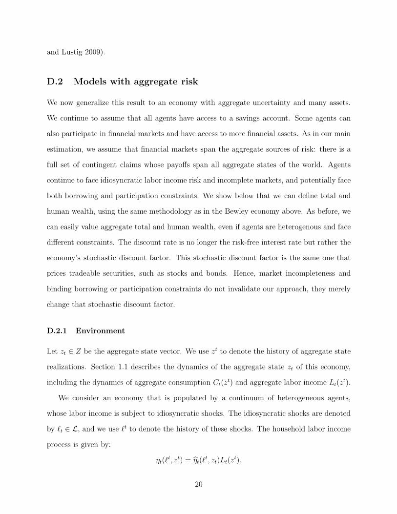
and Lustig 2009).
D.2 Models with aggregate risk
We now generalize this result to an economy with aggregate uncertainty and many assets.
We continue to assume that all agents have access to a savings account. Some agents can
also participate in financial markets and have access to more financial assets. As in our main
estimation, we assume that financial markets span the aggregate sources of risk: there is a
full set of contingent claims whose payoffs span all aggregate states of the world. Agents
continue to face idiosyncratic labor income risk and incomplete markets, and potentially face
both borrowing and participation constraints. We show below that we can define total and
human wealth, using the same methodology as in the Bewley economy above. As before, we
can easily value aggregate total and human wealth, even if agents are heterogenous and face
different constraints. The discount rate is no longer the risk-free interest rate but rather the
economy’s stochastic discount factor. This stochastic discount factor is the same one that
prices tradeable securities, such as stocks and bonds. Hence, market incompleteness and
binding borrowing or participation constraints do not invalidate our approach, they merely
change that stochastic discount factor.
D.2.1 Environment
Let zt ∈ Z be the aggregate state vector. We use zt to denote the history of aggregate state
realizations. Section 1.1 describes the dynamics of the aggregate state zt of this economy,
including the dynamics of aggregate consumption Ct(zt) and aggregate labor income Lt(z
t).
We consider an economy that is populated by a continuum of heterogeneous agents,
whose labor income is subject to idiosyncratic shocks. The idiosyncratic shocks are denoted
by ℓt ∈ L, and we use ℓt to denote the history of these shocks. The household labor income
process is given by:
ηt(ℓt, zt) = ηt(ℓ
t, zt)Lt(zt).
20

Let Φt(zt) denote the distribution of household histories ℓt conditional on being in aggregate
node zt. The labor income shares η aggregate to one:
∫ηt(ℓ
t, zt)dΦt(zt) = 1.
D.2.2 Trading in securities markets
A non-zero measure of these households can trade bonds and stocks in securities markets
that open every period. These households are in partition 1. We assume that the returns of
these securities span Z. In other words, the payoff space is RZ×t in each period t. Households
in partition 2 can only trade one-period riskless discount bonds (a cash account). We use Aj
to denote the menu of traded assets for households in segment j ∈ 1, 2. However, none of
these households can insure directly against idiosyncratic shocks ℓt to their labor income by
selling a claim to their labor income or by trading contingent claims on these idiosyncratic
shocks.
D.2.3 Law of one price
We assume free portfolio formation, at least for some households, and the law of one price.
There exists a unique pricing kernel Πt in the payoff space. Since there is a non-zero measure
of households that trade assets that span zt, it only depends on the aggregate shocks zt.
Formally, this pricing kernel is the projection of any candidate pricing kernel on the space
of traded payoffs X t = RZ×t:
Πt
Πt−1= proj(Mt|RZ×t).
We let Pt be the arbitrage-free price of an asset with payoffs Dit:
P it = Et
∞∑
τ=t
Πτ
Πt
Diτ , (D.3)
for any non-negative stochastic dividend process Dit that is measurable w.r.t zt.
21

Household Problem We adopted the approach of Cuoco and He (2001). We let agents
trade a full set of Arrow securities (contingent on both aggregate and idiosyncratic shock
histories), but impose measurability restrictions on the positions in these securities.
After collecting their labor income and their payoffs from the Arrow securities, households
buy consumption in spot markets and take Arrow positions at+1(ℓt+1, zt+1) in the securities
markets subject to a standard budget constraint:
ct + Et
[Πt+1
Πtat(ℓ
t+1, zt+1)
]+
∑
j∈Aj
P jt s
jt+1 ≤ θt,
where s denotes the shares in a security j that is in the trading set of that agent. In the
second term on the left-hand side, the expectations operator arises because we sum across all
states of nature tomorrow and weight the price of each of the corresponding Arrow securities
by the probability of that state arising. Wealth evolves according to:
θt+1 = at(ℓt+1, zt+1) + ηt+1 +
∑
j∈Aj
[P jt+1 +Dj
t+1
]sjt ,
subject to a measurability constraint:
at(ℓt+1, zt+1) is measurable w.r.t. Aj
t(ℓt+1, zt+1), j ∈ 1, 2,
and subject to a generic borrowing or solvency constraint:
at(ℓt+1, zt+1) ≥ Bt(ℓ
t, zt).
These measurability constraints limit the dependence of total household financial wealth
on (zt+1, ℓt+1). For example, for those households in partition 2 that only trade a risk-free
bond, A2t (ℓ
t+1, zt+1) = (ℓt, zt), because their net wealth can only depend on the history of
aggregate and idiosyncratic states up until t. The households in partition 1, who do trade
22

in stock and bond markets, can have net wealth that additionally depends on the aggregate
state at time t + 1: A1t (ℓ
t+1, zt+1) = (ℓt, zt+1).
D.2.4 Pricing of household human wealth
In the absence of arbitrage opportunities, we can eliminate trade in actual securities, and
the budget constraint reduces to:
ct + Et
[Πt+1
Πt
at(ℓt+1, zt+1)
]≤ at−1(ℓ
t, zt) + ηt.
By forward substitution of at(ℓt+1, zt+1) in the budget constraint, and by imposing the
transversality condition on household net wealth:
limt→∞
Πtat(ℓt, zt) = 0,
it becomes apparent that the expression for financial wealth is :
at−1(ℓt, zt) = Et
[∞∑
τ=t
Πτ
Πt(cτ (ℓ
τ , zτ )− ητ (ℓτ , zτ ))
]
= Et
[∞∑
τ=t
Πτ
Πt
cτ (ℓτ , zτ )
]−Et
[∞∑
τ=t
Πτ
Πt
ητ (ℓτ , zτ )
].
The equation states that non-human wealth (on the left) equals the present discounted value
of consumption (total wealth) minus the present discounted value of labor income (human
wealth). The value of a claim to c − y is uniquely pinned down, because the object on the
left-hand side is traded financial wealth.
D.2.5 Pricing of aggregate human wealth
Let Φ0 denote the measure at time 0 over the history of idiosyncratic shocks. The (shadow)
price of a claim to aggregate labor income at time 0 is given by the aggregation of the
23
valuation of the household labor income streams:
∫E0
[∞∑
t=0
Πt
Π0
(ct(ℓ
t, zt)Ct(zt)− ηt(ℓ
t, zt)Lt(zt))]dΦ0
= E0
[∞∑
t=0
Πt
Π0
∫ (ct(ℓ
t, zt)dΦt(zt)Ct(z
t)− ηt(ℓt, zt)dΦt(z
t)Lt(zt))],
= E0
[∞∑
t=0
Πt
Π0[Ct(z
t)− Lt(zt)]
],
where we have used the fact that the pricing kernel Πt does not depend on the idiosyncratic
shocks, the labor income shares integrate to one∫ηt(ℓ
t, zt)dΦt(zt) = 1, and the consumption
shares integrate to one∫ct(ℓ
t, zt)dΦt(zt) = 1, in which Φt(z
t) is the distribution of household
histories ℓt conditional on being in aggregate node zt.
Under the maintained assumption that the traded assets span aggregate uncertainty,
this implies that aggregate human wealth is the present discounted value of aggregate labor
income and that total wealth is the present discounted value of aggregate consumption, and
that the discounting is done with the projection of the SDF on the space of traded payoff
space. Put differently, the discount factor is the same one that prices tradeable securities,
such as stocks and bonds. This result follows directly from aggregating households’ budget
constraints. The result obtains despite the fact that human wealth is non-tradeable in this
model, and therefore, markets are incomplete.
Since the above argument only relied on iterating forward on the budget constraint,
we did not need to know the exact form of the equilibrium SDF. Chien, Cole, and Lustig
(2011) show that the SDF in this environment depends on the evolution of the wealth
distribution over time. More precisely, for each agent, one needs to keep track of a cumulative
Lagrange multiplier, which changes whenever the measurability constraints or the borrowing
constraints bind. One cross-sectional moment of these cumulative multipliers suffices to
keep track of how the wealth distribution affects asset prices. Because of the law of large
numbers, those moments only depend on the aggregate history zt. Similar aggregation results
24

are derived in Constantinides and Duffie (1996) and in the limited commitment models of
Lustig (2007) and Lustig and Van Nieuwerburgh (2007). To sum up, in the presence of
heterogeneous agents who cannot trade idiosyncratic labor income risk, there is an additional
source of aggregate risk that captures the evolution of the wealth distribution. However, asset
prices will fully reflect that source of aggregate risk so that our procedure remains valid in
such a world.
D.2.6 No spanning
If the traded payoffs do not span the aggregate shocks, then the preceding argument still
goes through for the projection of the candidate SDF on the space of traded payoffs:
Π∗t
Π∗t−1
= proj (Mt|Xt) .
We can still price the aggregate consumption and labor income claims using Π∗. In this case,
the part of non-traded payoffs that is orthogonal to the traded payoffs, may be priced:
Et
[(Ct+1 − proj
(Ct+1|X t+1
))Π∗
t+1
]6= 0,
Et
[(Yt+1 − proj
(Yt+1|X t+1
))Π∗
t+1
]6= 0,
where we assume that X includes a constant so that the residuals are mean zero. In the
main text, we compute good-deal bounds.
25