CMPO Working Paper Series No. 04/097

CMPO is funded by the Leverhulme Trust.

The Wage Scar from Youth Unemployment

Paul Gregg1

and Emma Tominey2

1CEP, LSE; CMPO and Department of Economics, The University of Bristol 2CMPO, The University of Bristol

February 2004

Abstract In this paper we utilise the National Child Development Survey to analyse the impact of unemployment during youth upon the wage of individuals up to twenty years later. We find a large and significant wage penalty, even after controlling for educational achievement, region of residence and a wealth of family and individual specific characteristics. We employ an instrumental variables technique to ensure that our results are not driven unobserved individual heterogeneity. Our estimates are robust to the test, indicating that the relationship estimated between youth unemployment and the wage in later life is a causal relationship. Our results suggest a scar from early unemployment in the magnitude of 12% to 15% at age 42. However, this penalty is lower, at 8% to 10%, if individuals avoid repeat incidence of unemployment. Keywords: Youth Unemployment, Scarring, Cost of Job Loss JEL Classification: J31, J64

Acknowledgements We would like to thank the Leverhulme Trust for financial and participants at a CMPO internal seminar for comments and suggestions. The usual disclaimers apply. Thanks to the Dynamic Approach to Europe's Unemployment Programme (DAEUP) of the EU for funding. Address for Correspondence Department of Economics University of Bristol 12 Priory Road Bristol BS8 1TN P.Gregg@bristol.ac.uk

1

1. Introduction

Whilst a spell of unemployment will generate a direct loss of income, studies examining

the full cost of job loss show that a period of unemployment imposes disadvantages

individuals above and beyond this direct cost. For example, Jacobson et al (1993) provide

evidence of a wage loss associated with displacement from employment which

commences up to three years prior to the date of displacement and is still evident five

years following. Furthermore, according to Huff Stevens (1997), in the post-displacement

period a person is made much more vulnerable to repeated incidence of unemployment.

Stewart (2000), suggests that low pay and higher incidence of job loss are correlated to

create a low-pay-no-pay cycle; whereby individuals located low down on the income

distribution face a relatively high risk of becoming unemployed. This combined with the

widening gap between pre- and post- displacement wages in the UK (Nickell et al. 2002)

results in long lasting negative effects from a spell of unemployment. The deterioration of

labour market prospects stemming directly from an initial spell of unemployment is

sometimes termed a ‘scar’; and can come in the form of either higher unemployment or a

lower subsequent wage or a combination of both.

There are potential policy implications related to evidence of scarring. Whilst the lowest

exit rates from unemployment fall upon older, less educated individuals, intervention

may be better directed towards the youth, if the evidence suggests that unemployment

imposes a substantial scar upon individuals, which they carry for much of their future

labour market experience. As with the old adage, ‘prevention is better than cure’, the

prevention of extended periods of unemployment as individuals gain their first footholds

in the labour market may reduce these long-lasting disadvantages. However, an

econometric problem exists whereby the fixed individual characteristics which make

someone prone to unemployment as a youth, will also drive later unemployment and poor

wages. Further, these characteristics may well be poorly observed in conventional

databases or difficult to observe at all, such as motivation, self-confidence and

expectations. Consequently, the relationship between early unemployment and later

outcomes may not be causal but reflect heterogeneity. If this is the case, policy aimed at

reducing the incidence or duration of unemployment will be misdirected and the vast

2

inequalities in life chances will remain.

We use the National Child Development Survey (NCDS) database to explore evidence of

scarring in the form of persistently lower wages from a person’s youth unemployment

experience. We look at how these scars evolve in terms of the initial impact on wages and

subsequent recovery and the countervailing impact of repeat incidence of job loss from

entry into the labour market up to age 42. Hence, the relationship between youth

unemployment and the cumulative history from age 23 to 42 is explored. The NCDS has

an expanse of information on factors often unobservable in other data, such as the cohort

members ability (literacy, numeracy and intelligence tests) and detailed family

background, as well as information upon their educational, occupational and economic

achievements during their lifetime. However there exists an evaluation problem. Any

relationship we observe between youth unemployment and the subsequent wage may not

be causal. If unobservable characteristics of cohort members drive early unemployment

experiences and the later wages, our results will be biased upwards. Therefore to ensure

the estimated relationship is truly causal we employ the Instrumental Variables technique.

The unemployment rate prevalent locally for individuals aged 16 is employed to

instrument youth unemployment in the wage equation for individuals aged 33. The

intuition is that at such a young age, the individuals have little autonomy over their area

of residence, thus the personal characteristics of the individuals are removed from the

equation. Further, the local rate of unemployment certainly plays a role in determining

experiences of unemployment. We conclude that unobserved heterogeneity does not

create a bias. Thus our evaluation of the scarring effect of youth unemployment does

estimate the true relationship.

The research in this paper concludes that youth unemployment does indeed impose a

wage scar upon individuals, in the magnitude of 12% to 15% at age 42. However, this

penalty is lower, at 8% to 10%, if individuals avoid repeat incidence of unemployment.

The structure of the analysis of the wage scar from youth unemployment is as follows.

The literature surrounding this topic is evaluated in section 2. Section 3 details the data

set employed to tackle the issue at hand. The methodology adopted is described in section

3

4. The results are analysed in section 5 with relevant tables. Following from this, section

6 concludes and discusses the current labour market policies and the scope for future

policies, based upon these results.

2. Existing literature

It is obvious that a period of job loss reduces a persons current income. However the

detriment may be much longer lasting if unemployment carries a scar. Scarring is a

causal link between unemployment history and a negative future experience in the labour

market. The literature on the effects from scarring are highlights a twofold impact;

damaging the individual’s future employment prospects and/or lowering their subsequent

earnings; effects which potentially may last for the individual’s entire remaining working

lifetime.

A number of economic theories can predict scarring. Following the intuition of Becker

(1975), although general skills raise a worker’s marginal productivity in all different

firms and sectors, firm specific skills are non-transferable and thus increase the worker’s

marginal productivity only in the firm providing the investment. A consequence of

unemployment is the depreciation of general skills and the loss of firm specific skills.

The worker will therefore receive a wage lower on return to the labour market than that

received prior to the spell of unemployment. However, re-entry into the labour market

will initiate further accumulation of human capital and hence, as long as there are

diminishing returns to extra tenure, the scarring effects will only be temporary.

In standard unemployment Search Theory, unemployment that is a consequence of an

inappropriate match between the employer and employee will have a positive effect on

subsequent wages. Durations of unemployment are used for job search and thus improve

the likelihood of a good employer-employee match in subsequent jobs. However

Pissarides (1994) extends these models to include on-the-job search and here, with

dispersion in firm productivity, low quality firms recruit the unemployed but lose them to

better paying higher productivity firms. Displacement from a good job means a high

probability of return to a lower quality one and hence a cost-of-job loss. Part of these

4

costs will be permanent if the worker remains in the low wage sector to retain firm

specific human capital which would be lost on a switch to a better paying firm. Theories

of dynamic monopsony would create similar predictions (see Manning 2003 for a

discussion).

In a similar vein, if the employer ex-ante has imperfect information on the workers

quality, they will rationally seek more information ex-post to observe worker potential.

This leads to an initially lower wage on entry into a job. By observing the worker over

time to improve their knowledge of the worker’s productivity, information is revealed to

the firm but diffuses to other firms through actions from the employer, such as promoting

or firing the employee. Unemployment is then an example of a negative signal, which

carries a stigma effect as employers pick up on actions of other employers and view

unemployed job seekers as having lower average quality to employed job seekers.

Accordingly, unemployment will scar a worker throughout their entire future labour

market experience unless they can successfully signal their true quality.

Over the past decade, empirical economic studies have sought identification of the

scarring effect from unemployment by observing wages in the periods immediately

preceding and following the spell for workers where the displacement can be reasonably

thought to be exogenous to their quality. Rhum (1991) finds significant and negative

long-term effects on wages from periods spent in unemployment. Workers displaced at

the time of observation were more than twice as likely to have 25% lower wages and

experience on average 6 times more weeks out of work. Rhum also compares a control

group of non-displaced workers to a group of displaced workers in the three years prior to

displacement and four years following and finds that, whilst in the long run the

employment disadvantage diminishes, the wage penalty was large and persistent.

Jacobson et al (1993) contribute to the identification of the cost of job loss by detecting

an earnings loss three years prior to displacement using administrative records from

Pennsylvania. At the date of displacement there will be a dramatic drop, followed by a

quick recovery and 5 years after displacement, individuals had 25% lower earnings,

5

compared to non-displaced workers. Stevens (1997) also suggests that much of the cost

of job loss is permanent. Thus in order to prevent underestimating the scar it is necessary

to consider the full cost of job loss from unemployment. Stevens identifies multiple job

loss as a key driving force behind the permanent scarring effects of unemployment,

stating that if individuals can avoid falling into unemployment more than once, they will

face a good chance of recovery.

The UK literature explores the effects of unemployment more generally rather than

focusing on workers displaced in a major layoff, but show similar findings. Nickel et al.

(2002) report for the UK that the cost of job loss rose through the 1980s as wage

inequality grew. They also explore the impact of repeated job loss and suggest that repeat

job loss results in smaller wage penalties approximately half of that of the first incidence.

Arulampalam (2001) uses longitudinal data from the British Household Panel Survey

(BHPS) and support the findings that the cost of job loss are long-term and that second or

subsequent interruptions are less harmful than the first. Gregory and Jukes (2001) utilise

the combined information from two longitudinal datasets: New Earnings Survey Panel

Dataset (NESPD) and Joint Unemployment and Vacancies Operating System (JUVOS).

Their results suggest that the impact effect of job loss is short lived but the effect of

duration in the unemployment spell persist and are also strong in a second spell. Borland

et al. (2002) show that when a worker displaced from their job finds a new job during the

notice period of redundancy, therefore experiencing no unemployment, do not suffer

these wage falls.

Looking in particular at the scar imposed upon an individual from youth unemployment,

Gregory and Jukes explore variation across age groups and suggest that the impact effect

is more marked with older workers but the duration effects are more substantial for the

young. Gregg (2001) uses NCDS to analyse scarring in terms of future employment

prospects. Specifically Gregg asks whether the cumulated unemployment experience up

to the age of 23 drives unemployment in subsequent years. NCDS provides a wealth of

information on individuals and despite controlling for many observable characteristics of

individuals, Gregg identified persistent effects from youth unemployment. In addition,

6

an Instrumental Variables technique identifies whether this relationship is causal or

resulting from unobserved heterogeneity. The results, suggesting that no bias was

detected, lead to the conclusion that unemployment does causally scar individuals in

terms of their future employment.

A general consensus between these authors is that an unemployment spell consistently

imposes a wage scar upon individuals that persist. However, these studies rarely follow

individuals for more than 5 years or so. Although multiple spells of unemployment harm

individuals, results indicate that the first spell carries the most significant scar but the

impact of longer durations apply to all spells. Stevens (1997) suggests that a substantial

part of the reason for persistent effects is that repeat incidence inhibits wage recovery and

Gregg (2001) suggest that a spell of unemployment causally increases the likelihood of

repeat job loss or multiple spells. This present paper is closest in spirit to Stevens in that

we use the NCDS to track the impact of youth unemployment on earnings up to age 42,

thus we look for adverse effects from unemployment after 19 to 26 years and we explore

how such penalties diminish over that period and the role for further unemployment in

preventing recovery.

3. Data set

To show the impact that youth unemployment has upon an individual’s future experience

in the labour market, we utilise the National Child Development Survey (NCDS), a

longitudinal birth cohort pane l dataset. The NCDS children were those born in the week

3-9 March, 1958 living in Great Britain. Information was collected on the cohorts on

characteristics including gender, race, region of birth and whether the parents are

married. Subsequently, infor mation has been collected on these cohorts at ages 7 (1965),

11 (1969), 16 (1974), 23 (1981), 33 (1991) and 42 (1999/2000); creating what

approximates to a half-life time history of the individuals.

During the survey, information was gathered not only from the individuals themselves.

The parents were interviewed on topics such as their expectations and aspirations for

their child’s educational and employment prospects, their smoking, working and personal

7

relationship habits and the child’s health. Levels of financial difficulty were assessed and

anxiety traits of the children recorded, for instance whether the child experienced

depression or wet the bed. Further, the child’s ability is observed through a substantial

number of tests administered to the children, including drawing and copying, reading,

comprehension, mathematics and non-verbal reasoning (akin to IQ). Finally, details of

the cohort members as adults was collected at ages 23, 33 and 42 adding insight into the

individual’s record of crime, their family statistics (number of children, divorce) and their

educational and employment histories.

4. Methodology

Our interest lies in the extent to which youth unemployment scars an individual in terms

of their subsequent wage. Youth unemployment is defined as a period of unemployment

covering the ages 16-23, i.e. as the cohort members are first able to enter the labour

market. Individuals pursuing further education into their twenties will not provide a

representative picture of youth experience in the labour market, thus the sample is limited

to individuals with an employment history lasting more than 24 months between age 16

and 23. We attempt to identify the non-linear relationship between youth unemployment

and the subsequent wage, grouping the youth unemployment experience into six

categories: zero months, 1 – 2 months, 3 – 4 months, 5 – 6 months, 7 – 12 months and

13+ months. We analyse the wage scar for those with youth unemployment relative to

the counterfactual group experiencing no youth unemployment. The dependent variable

of the tests is the natural log of the wage reported by the cohort members: we analyse this

at three periods in their life, age 23, 33 and 42. The analysis of the wage scar at each

stage requires a sample constraint that we examine only those reporting a wage at the

relevant age 1.

The data from NCDS is combined with information on region of residence and ward level

unemployment rates from Census data in 1971 and 1991, for the purpose of employing

the Instrumental Variables technique to test for potential heterogeneity manifested in the

1 A summary of characteristics for individuals reporting a wage at different periods of observation is given in Appendix A.1

8

data.

Heterogeneity

We aim to examine the scar from unemployment experience before the age of 23 upon

the subsequent wage received up to the age of 42. Any unobserved heterogeneity

remaining in the results which is correlated with both unemployment and wages will

create an upward bias to the estimates of the impact of preceding unemployment.

Formally, individual i's wage experience at time t (Wit) is a function of their

unemployment experience up to the age of 23 (Uit -1), heterogeneity (Zit) and an error term

(Eit).

Wit = Uit -1 + Zit + Eit (1)

Heterogeneity is a set of non-time varying observable characteristics of the individual i

(Ai) including gender, family background and child ability and unobservable

characteristics (Bi), which may capture expectations, aspirations or self -confidence, and

an error term (ξit).

Zit = Ai + Bi + ξit (2)

The consequence of failure to take account of heterogeneity is the belief of a strong

relationship between unemployment and subsequent wages when, in truth it is not the

experience of unemployment per se that results in lower wages, but the unobserved

heterogeneity. This will result in either an omitted variable bias, or a violation of the

OLS assumption that the coefficient Uit -1 is correlated with the error term2. Subsequently

OLS estimation of Uit -1 will be biased. Therefore the assessment of the wage scar created

from youth unemployment is a two stage task: First, identify the relationship between

months of unemployment experienced before the age of 23 and the individual’s

subsequent wage. Second, examine whether this relationship is causal; a prerequisite for

scarring.

2 i.e. that correlation(Uit-1, Eit) = 0

9

Controlling for heterogeneity

Utilising NCDS

The plethora of information contained in NCDS is certainly an advantage in the task of

isolating a causal relationship between youth unemployment and the subsequent wage.

Firstly, it is possible to include variables into the model to account for educational

achievement and region of residence between 16-33 (reported at 16, 22 and 33). These

additions are a necessity in any reliable wage equation; an individual’s wage is at least in

part driven by educational attainment and, with variations in levels of employment across

regions and therefore variations in wages, it is vital to control for region. Although we

can condition on gender we choose to estimate the scar separately as the experience of

males and females within the labour market is often very different. Tracing a cohort

through various stages of their lives means that it is not possible to include age as an

explanatory variable of the model.

Obtaining information on the variables noted so far – months spent unemployed,

educational attainment and region – is relatively straight forward. However, the crucial

advantage of NCDS is the information on variables that are often unobservable, such as

school attendance, ability and childhood deprivation. These variables, although usually

unmeasured, certainly have the potential to inf luence the individual’s experience within

the labour market later in life. We limit the analysis to those variables thought influential

to the economic experience of the cohort. Thus, following Gregg (2001), we define a

group of variables specific to the individual’s family background and a group of variables

pertinent to the individual.

The family background characteristics include whether the parents stayed on at school

past age 16 (which could proxy ambitions or expectations of the parent and child), if the

cohort member is non-white, whether the child was exposed to financial deprivation or

put into care of the local authority and the income received by the household at age 16.

The individual specific variables incorporate negative anxiety traits at age 7 (for example

depression), low school attendance (truancy), sickness, scores on various school tests, for

example vocabulary IQ and mathematics (which proxy for ability) and whether the child

10

ever had educational special needs. If the individual and family specific characteristics

are creating an omitted variable bias in the relationship between youth unemployment

and subsequent wages, the coefficient of unemployment will fall with the introduction of

these background variables.

Econometric techniques

However detailed the set of child and family information available, one or more

important background characteristic may have been excluded from the dataset or badly

measured. Therefore it is necessary to further control for the unobserved heterogeneity,

through econometric techniques. Three main methods are generally adopted in the

scarring or cost-of-job-loss literature.

Difference-in-difference

A target group is exposed to a policy change aimed eliminating any potential scar from

unemployment by preventing its occurrence. The results of the group are recorded and

compared to a benchmark group not affected by job loss, conditional on observed

characteristics. The pre-displacement (or unemployment spell) wage should capture any

unobserved characteristics that influence wages so that the change in the wage compared

across affected and unaffected groups is net of such unobserved differences. Nickell et al.

(2002) and Gregory and Jukes (2001) opted for the difference-in-difference to separate

heterogeneity from true scarring. However, if the reason for job loss was due to the pre-

unemployment wage being too high as a result of a poor match, then even this estimate

will be biased. Hence the cost-of-job loss literature tends to include in the sample cases

where the displacement can reasonably be thought to be exogenous, for instance where a

plant has closed or had mass layoffs. Here the event is plausibly exogenous to the worker

quality. Unfortunately such data is not available for the UK.

Assume functional form

A number of studies estimating structural dependence in unemployment (reviewed by

Machin and Manning, 1999) attempt to separate dependence from heterogeneity by

making assumptions about the likely distribution of such heterogeneity. Lancaster (1990)

11

states that this method requires certain heroic assumptions regarding the parametric

specification of heterogeneity. However, such assumptions about the functional form of

the model may lead to misspecification, if they are incorrect. Indeed, Heckman and

Borjas (1980) argue that, although the a priori assumptions are necessary for empirical

investigations into scarring, “In most cases, such assumptions usually cannot be justified

by an appeal to economic theory.”

Instrumental variables

For the Instrumental Variables technique it is necessary to identify as an instrument some

variable which drives the unemployment experience - the endogenous factor - but which

is exogenous to the individual themselves. If it is true that the characteristics which drive

youth unemployment also drive low wages, rather than (or as well as) the experience of

unemployment per se acting as the driving force, then the instrument must capture the

effect of these characteristics. This will ensure that any results we observe, in terms of

the relationship between unemployment and wages, is causal. Heckman and Borjas

(1980) cite the Instrumental Variables method as advantageous and accordingly it is the

technique adopted in this study. A criticism of the instrumental variables technique is the

difficulty in identifying a valid instrument. However, with the nature and expanse of the

longitudinal data available, identifying an instrument is simplified. With impetus from

Gregg (2001), the unemployment rate prevalent locally for individuals aged 16 is

employed to instrument youth unemployment in the wage equation for individuals aged

33. The intuition is that at such a young age, the individuals have little autonomy over

their area of residence, thus the personal characteristics of the individuals are removed

from the equation. Further, the local rate of unemployment certainly plays a role in

determining experiences of unemployment.

The local rate of unemployment when the individuals are aged 33 is included as an

endogenous variable. Individuals are sorted into areas, which crudely can be classified

into high and low income areas according to their earnings. Furthermore, the impact of

recessions of 1980’s and 1990’s upon regions of the UK was not evenly distributed

geographically. Thus to remove any correlation between unemployment after youth and

12

the instrument (as individuals may not have moved far away), local unemployment rates

in 1991 are controlled for. Consequently, local labour market conditions when the

individuals were aged 16 will not directly impact upon later unemployment conditional

upon local unemployment rates in 1991, except through scarring. A criticism of using the

local rate of unemployment or area of residence at age 16 is that rather than removing the

influence of heterogeneity from the equation, heterogeneity is just pushed back a

generation, as parents have an impact upon where the child lives as they enter the labour

market. Consequently it must be noted that there is a risk of the parents’ heterogeneity

creating a residual bias in the results but, as there is less than complete intergenerational

immobility in life chances, then the bias should be reduced.

5. Results

Summary of NCDS data

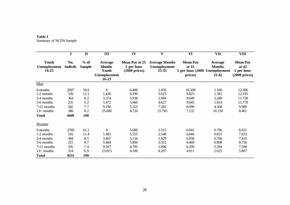
Table 1 describes the characteristics of the NCDS dataset, distinguishing between males

and females. The cohort members have been grouped into six categories, depending

upon the number of months spent unemployed between the age of 16-23: zero months, 1-

2 months, 3-4 months, 5-6 months, 7-12 months and 13+ months. The vast majority of

individuals – approximately 60% - experience no unemployment during their youth,

whilst of the remaining 40%, 11-12% reported being unemployed for only approximately

1½ months. However, one fifth of the sample individuals are subjected to 5+ months of

unemployment during their youth, with the hardest hit 8% clocking up some 26 months

unemployment as youths on average. There is an easily identifiable correlation between

unemployment during youth and in the subsequent decade (column V), although between

ages 33-42 (column VII) even the individuals with extensive youth unemployment are

rarely unemployed. This may, in part, reflect the fact that the period of 1991 to 2000 was

characterised by a sustained upswing.

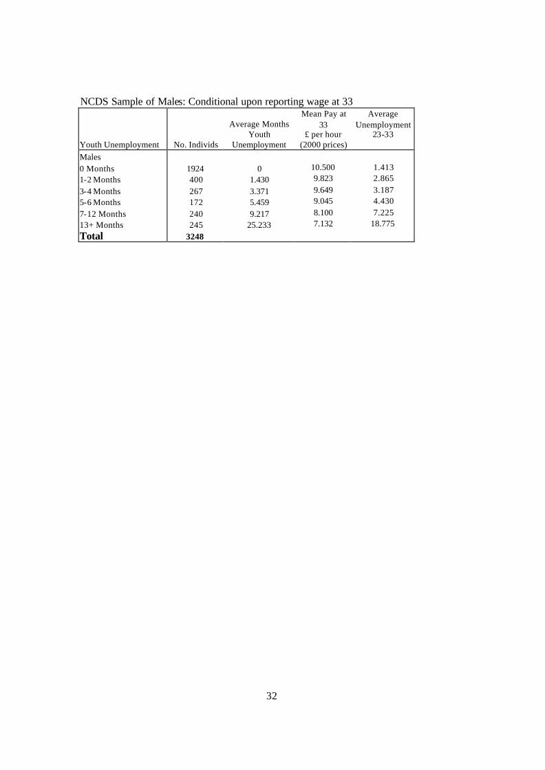
Immediately obvious from columns IV, VI and VIII is the trend for the mean wage of the

cohort to decline as youth unemployment accrues. Men carrying the worst history from

their youth labour market experience will be paid £4.00 per hour less twenty years later, a

30% penalty, compared to men with no youth unemployment. The wage gap is large for

13

men whether the wage is measured at age 23, 33 and 42. For women the penalty is

approximately £2.00 per hour at age 42 and is consistently slightly lower compared to

women with no youth unemployment than for men.

Wage scar at 23

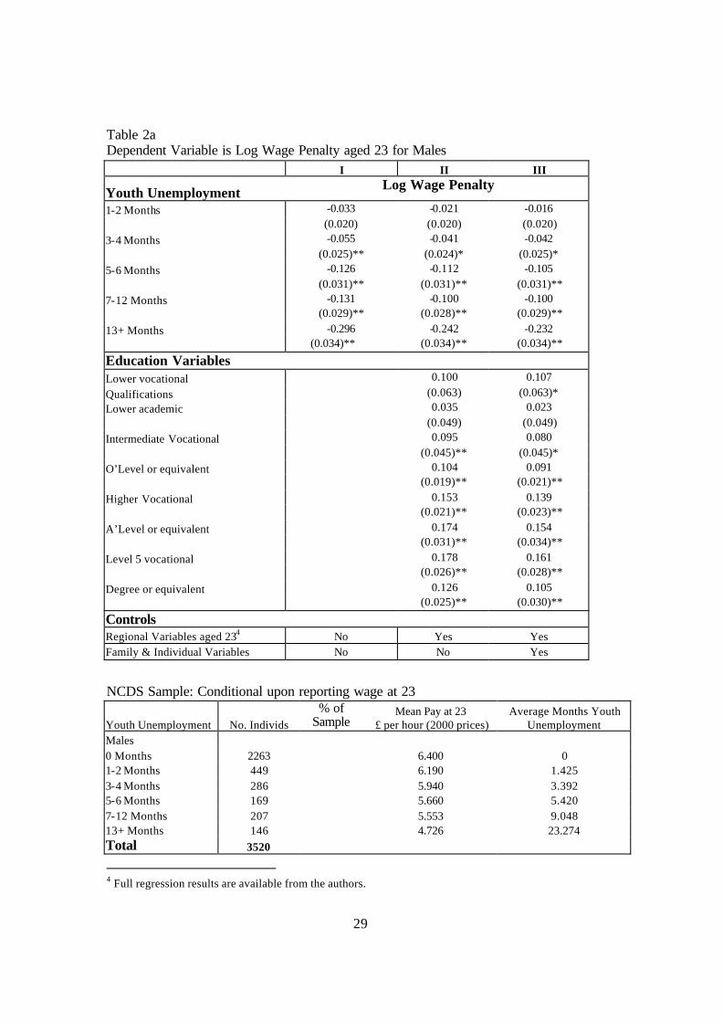
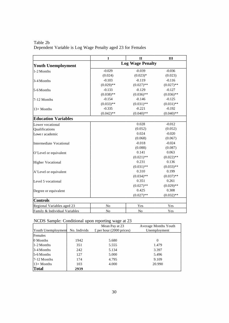
Tables 2a and b report the log wage scar at 23 for men and women respectively. Cohort

members are included in the analysis only if they report a wage at 23; details of the

restricted sample are given beneath the regression results. Almost 1,000 men and 1,500

women have been dropped from the sample, changing the composition so that individuals

with no history of youth unemployment have a somewhat greater representation and

those with 13+ months have almost half as much prevalence than in the whole sample.

Looking at column I, a large raw wage gap at 23 is evident between those experiencing

5+ months of unemployment compared to those with no or very little youth

unemployment. In the worst case scenario, compared to an individual with no youth

unemployment, a history of 13+ months of unemployment between the age of 16-23 is

associated with an average reduction in earnings of a 23 year old male by almost 30%

and the earnings of a 23 year old female by 35%.

Accounting for observable heterogeneity

Introducing controls for background characteristics in turn will identify the contribution

of each towards the wage gap at 23, revealing the upward bias omission these

background characteristics creates.

Education and region of residence at 23

Educational attainment is associated with different earning capacities, regardless of an

employment history. Relatively poorly qualified individuals achieve lower paid jobs and

tend to experience more unemployment. In addition, regions with higher unemployment

tend to have lower wages. Inclusion of controls for region and education are thus vital

initial conditions when calculating the impact of unemployment upon wages. It should,

however, be noted that at age 23, the returns to educational qualificat ions are not yet fully

14

apparent and the regional wage gaps are not strongly related to unemployment

differences. Column II of Tables 2a and b shows youth unemployment on the whole to

be less severe than the previous results suggested once education and region is taken into

account. Inclusion of region of residence does not change the scar a great deal. The

implied effect of 7-12 months unemployment on wages is reduced by just 3% for men

and 1% for women. The damaging consequence of 13+ months unemployment during

youth is reduced by just 5% for males and by over 10% for women once the educational

heterogeneity of the individuals is taken into account. These relatively small adjustments

probably reflect a muted educational premia among such a young cohort. Workers with

higher vocational qualifications or above are earning only between 13-18% if they are

men, although the wage premia of women at 23 is larger.

Family and individual specific characteristics

Whilst educational returns are low at age 23, it may be that other factors, correlated with

youth unemployment, are driving the observed variation in wages. The most obvious

candidates are ability unmeasured by qualifications and dimensions of parental

background. The NCDS unusually allows a serious attempt to control for many of these

characteristics. The ability of each individual, the aspirations of parents as to the

individual’s achievements, the parental involvement in raising the individual and the

physical and mental health of the individual, all of which are potential driving forces of

an individual’s earnings capacity can be controlled for. Column III of Table 2a and b

report that inclusion of a wealth of detail capturing the family and individual

heterogeneity does little to alter the wage scar reported above. Youth unemployment

experience appears to be one of biggest drivers of wage rates at age 23.

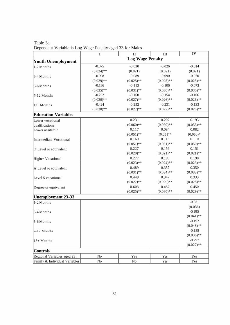
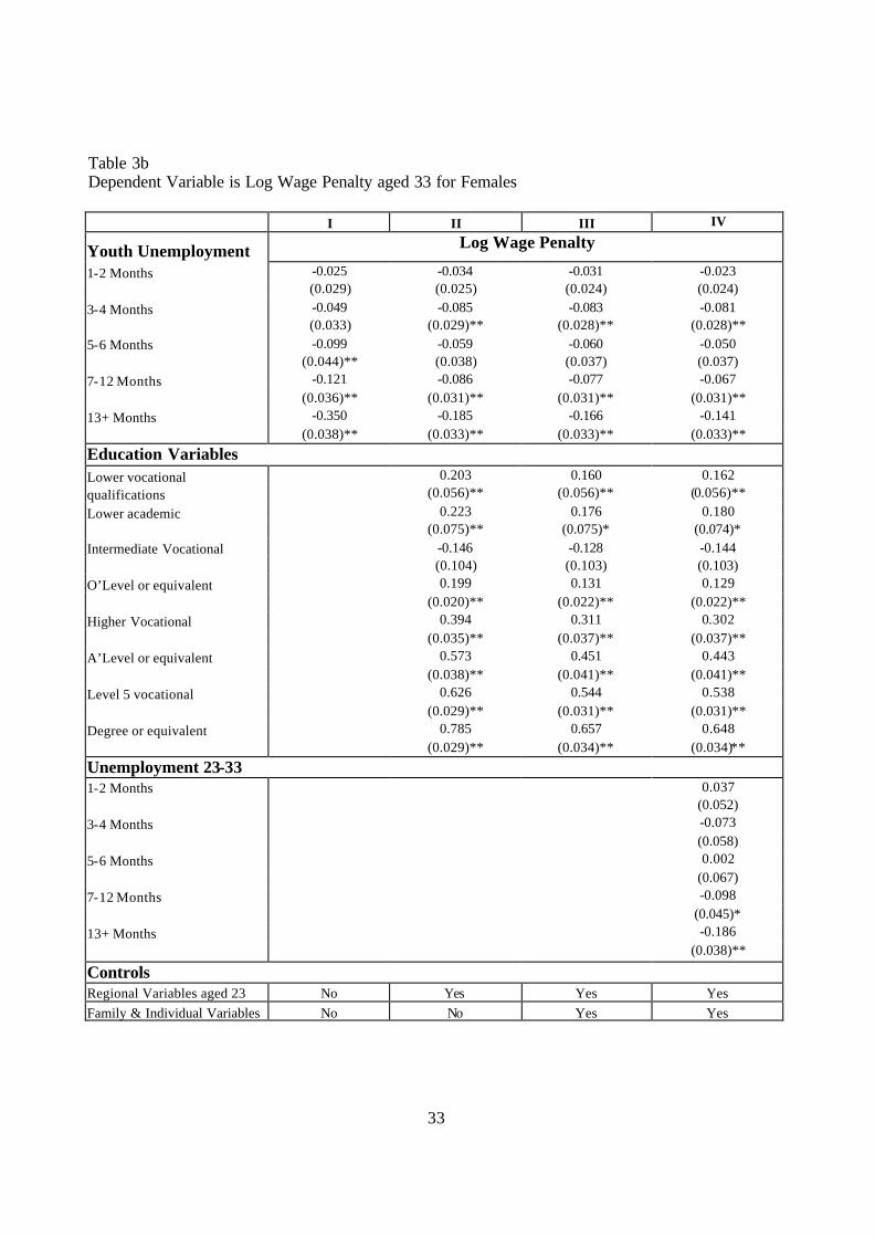
The wage scar at 33

The next stage of analysis steps ten years further into the individual’s lives, looking for

evidence of the wage scar evident at age 33. Tables 3a-3c detail the results which

evaluate the wage scar at age 33 and analyse how the scar changes between the age of 23

and 33. To analyse the scar present at age 33 it is necessary to restrict the sample of

evaluation to those reporting a wage at 33. The restriction excludes approximately 2,400

15

cohort members from the full sample, however the proportion of individuals within the

different classifications of youth unemployment is fairly similar to the original sample.

By age 33, the raw log wage penalty for males at every category of youth unemployment,

reported in column 1 has intensified relative to a full employment experience, compared

to ten years previously. It is broadly similar for women. Focusing upon the worst case

scenario, for a male reporting a history of 13+ months of youth unemployment, over the

years 23-33 the wage penalty has increased by over 10% to 42%.

Conditioning upon educational achievement and region of residence becomes much more

important as returns to education rise with age. The results in column II shows that

obtaining a degree will increase the wage at 33 by 60% for males and by nearly 80% for

females. In column II, we compare two individuals with an identical educational

background, inhabiting the same area but with a different labour market experience

during their youth. At age 33 we will still observe wage rates which have diverged for

these individuals. The wage of males tends to be lower by up to 25% at 33 and the

women’s by 18% among those with over a year worth of youth unemployment compared

to the individual with no youth unemployment. For men with 5 to 12 months

unemployment wages are 11-16% lower and 6-9% for women. Column III displays

results when controlling for family and individual specific cha racteristics. Again the log

wage penalty for experiencing some youth unemployment declines once these

characteristics were controlled for, but only marginally. Thus two males or females

identical in terms of their level of education, their region of residence, their parent’s

education and their IQ, literacy and numeracy test scores etc., will on average have an

earnings gap of 23% and 16% respectively resulting from a year of youth unemployment

for one individual. The conditional estimates of the wage penalty associated with youth

unemployment are now very similar at ages 23 and 33. This suggests little or no progress

in mitigating the impact of youth unemployment over the decade.

Column IV of Tables 3a and b introduce controls for unemployment experience between

the ages of 23 and 33. This conditions out the extent to which youth unemployment

16

experience is correlated with unemployment experience as young adults. It also

incorporates the repeat incidence of job loss - found to be important in the work of Gregg

(2001) and Stevens (1997) - into the true cost of job loss. Hence the counterfactual now

is the wage penalty associated with no youth unemployment given similar subsequent

unemployment experience. The wage penalties here associated with youth unemployment

are substantially lower for men but changes little for women as the persistence in patterns

of unemployment are much less prolific for women. The males within our sample

experiencing 3 to 6 months unemployment as youths but no extra unemployment after

age 23 have wage penalties of the order of 7%. For 7+ months the penalty increases to 11

to 13%. The penalties conditional on unemployment experience are now similar for men

and women. There is evidence of earnings recovery among those experiencing substantial

youth unemployment, if they avoid further exposure to unemployment. However, those

unemployed for more than 6 months as youths and again between age 23- 33 suffer very

large wage penalties. This finding raises a question about when the wage difference is

first evident. If lower ability or motivation is observed by employers but not picked up in

the data, then the wage at 23 may be lower for individuals who go on to experience

extensive later unemployment. Evidence to the contrary would suggest that lower paid

jobs are less stable and have scarring effects of their own, as suggested by Stewart

(2000).

We separate individuals experiencing at least 6 months of youth unemployment into two

groups: those in full employment in the decade following youth and those with some

unemployment (at least 3 months). There was no significant difference in the wage at 23

for the two groups of individuals3. Yet a person experiencing 7+ months of

unemployment between 23 and 33 has wages at 33 that are 16-30% lower for men and

10-19% lower for women. So those workers who go on to experience adult

unemployment had an insignificantly different wage at age 23 relative to other workers

with similar pre-23 characteristics but no later unemployment. This suggests that it is the

unemployment experience that induces scarring, rather than ability, unobserved by the

3 Coefficient for men with youth unemployment and some later unemployment was 0.0426 (0.0476). For women the coefficient was –0.0844 (0.0614).

17

researcher but apparent to employers, that drives down the wage received later in life.

Playing catch up

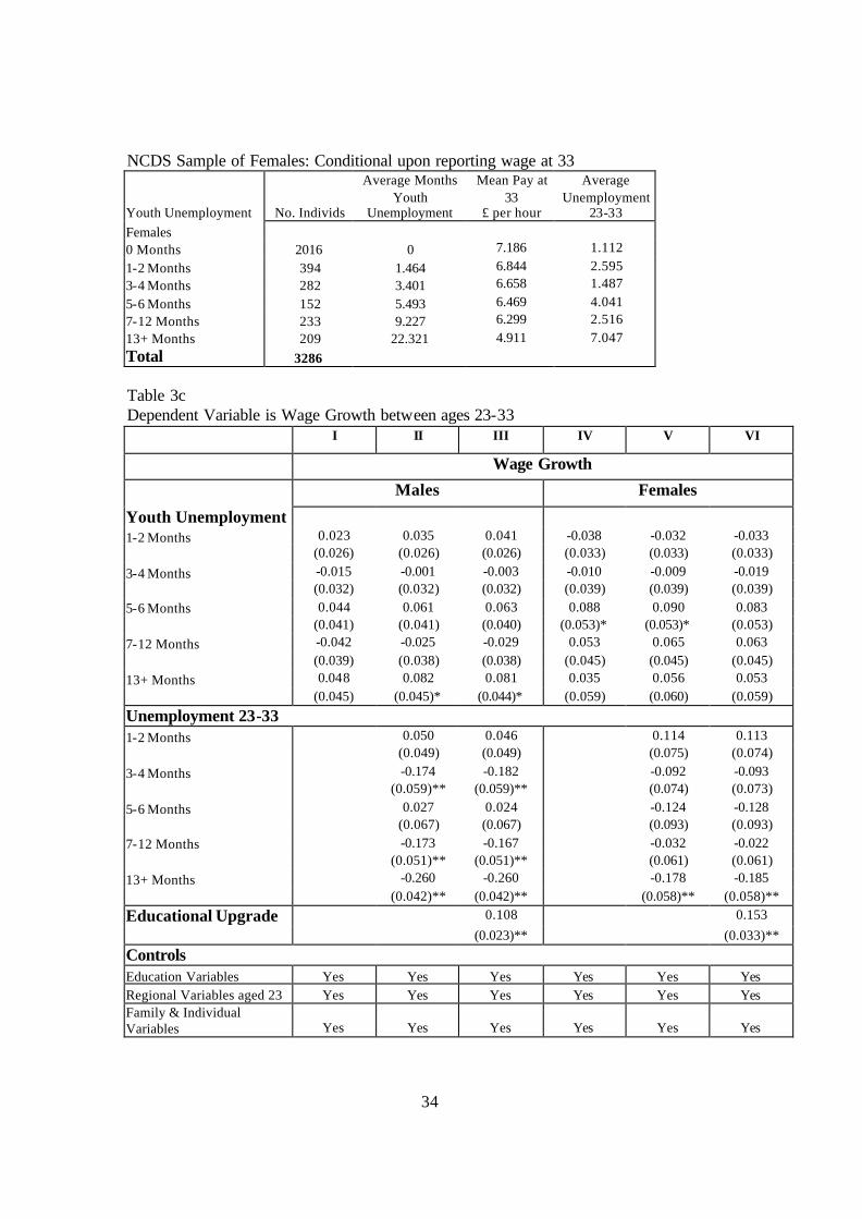
Table 3c explores the dynamics of the wage penalty between ages 23 and 33. This

requires both wages at 23 and 33 to be observed. This further restricts the sample,

especially among those with a substantial history of youth unemployment, as their wage

is less likely to be observed at 23. The wage growth equation differs from comparing the

wage gap level at 23 and 33 to the extent that those missing a wage at 23 can appear in

the wage equation at 33 and vice versa. So to explore the impact of this selection we

included a dummy variable which equals one if individuals report a wage at 23 and 0

otherwise into the equation for wages at 33 and a similar dummy for reporting a wage at

33 in the age 23 wage equation. This tests whether the sample population being dropped

by moving to a wage growth equation differs from the residual populations. Perhaps

unsurprisingly both sets of terms are positive. Men and women with an observed wage at

23 and at 33 have wages that are nearly 7-8% higher for given other characteristics at age

23, hence low wage jobs are generally less stable. Women reporting a wage at age 23 will

tend to receive a wage at 33 which is 15% higher for given characteristics. For men the

effect is smaller, at around 4%, however once we condition upon unemployment

experience between ages 23 and 33 the effect disappears.

The individuals not reporting a wage at either 23 or 33 are those spending relatively more

time unemployed as youths. The consequence in terms of selection in the wage growth

equation is that the picture of earnings progression for the high youth unemployment

groups will be altered by the selection criteria. For men, the bias of focusing analysis on

those reporting wages at both 23 and 33 results in the wage growth of those with

substantial youth unemployment being somewhat exaggerated. This is because the bias

is stronger at 23 than 33. For women, the picture is reversed.

Columns I and IV of Table 3c show the correlations between wage growth and youth

unemployment conditioning for education, region of residence and the family and

individual characteristics of the cohort members, for men and women respectively. The

18

results match implications of the above results that there is no significant catch-up for

individuals with a substantial amount of youth unemployment. Columns II and V control

for repeat unemployment between the age of 23 and 33 and suggest that there is wage

recovery among men experiencing over a year of youth unemployment. Pooling those

with 5+ months unemployment improves the precision of the estimated wage growth and

suggests modest recovery of around 5% for those who go on to experience little or no

further unemployment. These results again show how the common pattern of exposure to

further substantial unemployment continues to damage individuals with substantial youth

unemployment and on average prevents recovery among men. For women repeat

exposure is less of an issue.

Also utilising the NCDS, Gregg and Machin (2000) found that there are significant wage

returns from late achievement of educational qualifications. 18% of males and 12% of

females from our sample improve their educational achievement between 23-33 and

columns III and VI of Table 3c shows that a wage improvement of 11% for men and 15%

for women can be attributed to late educational development. The educat ional upgrade

variable was interacted with long-term youth unemployment (defined as a spell greater

than 4 months) and included into the previous equation to isolate any difference in the

ability to "catch up" for the more disadvantaged individuals. The size of the effect for

both genders is small and insignificant, indicating that regardless of an individual’s

employment experience in their early years of labour market activity, late educational

developers can improve their earnings potential. Thus there is a chance of weakening the

scar from youth unemployment through returning to education. However, such upgrading

is neither more common among those experiencing a lot of youth unemployment – the

target group – nor does it fully compensate for the loss of earnings resulting from the

youth unemployment.

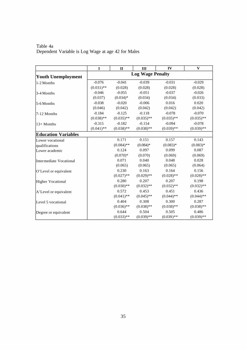
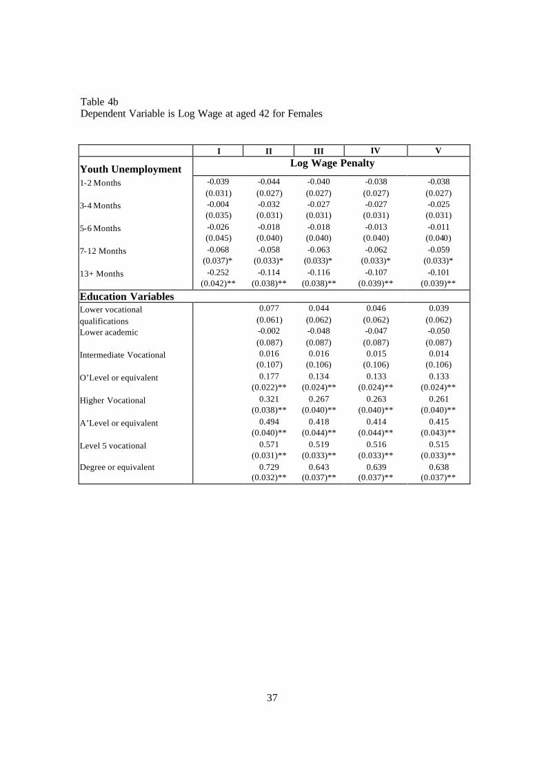
The wage scar at 42

More than twenty years after an event of unemployment has occurred, does the negative

impact remain? Tables 4a and 4b report the results for wages at age 42. The sample is

restricted to include those who report a wage at 42. Compared to the scar prevailing at

19

age 33, the raw wage penalty from youth unemployment observed when individuals are

aged 42 has weakened slightly. 13+ months of youth unemployment is associated with a

raw wage gap of approximately 30% at age 23 for men, which increases to 42% by age

33 and falls back to 32% by age 42. The overall picture seems slightly different for

women, whereby the wage penalty at age 23 is 34%, increasing marginally to 35% at 33,

but by age 42 falls to 25%. Education accounts for a large amount of the wage gap at 42,

as column II of Table 4a and b show: qualification to degree standard pushes wages up by

around 65-70%, relative to no qualifications. Column III adds family and individual

specific characteristics into the equation, with the intent of isolating the detriment from

youth unemployment upon the wage at 42, regardless of the individual themselves. The

fall in the log wage penalty is approximately 2% for males with an experience of youth

unemployment over 7 months, but is very small for females. These conditional estimates

of the wage penalty at age 42 are now much lower than at age 23 or 33. For males the

conditional wage gap, for over a year of unemployment before the age of 23, is 23% at

age 23 and 33 but just 15% at age 42. The pattern for shorter youth unemployment (3-12

months) shows similar shrinkage in the wage penalty. For women, the reduction in these

penalties is even more marked. For both men and women, only youth unemployment

over 6 months statistically is significantly negatively related to wages at age 42.

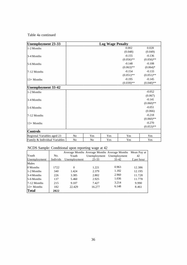
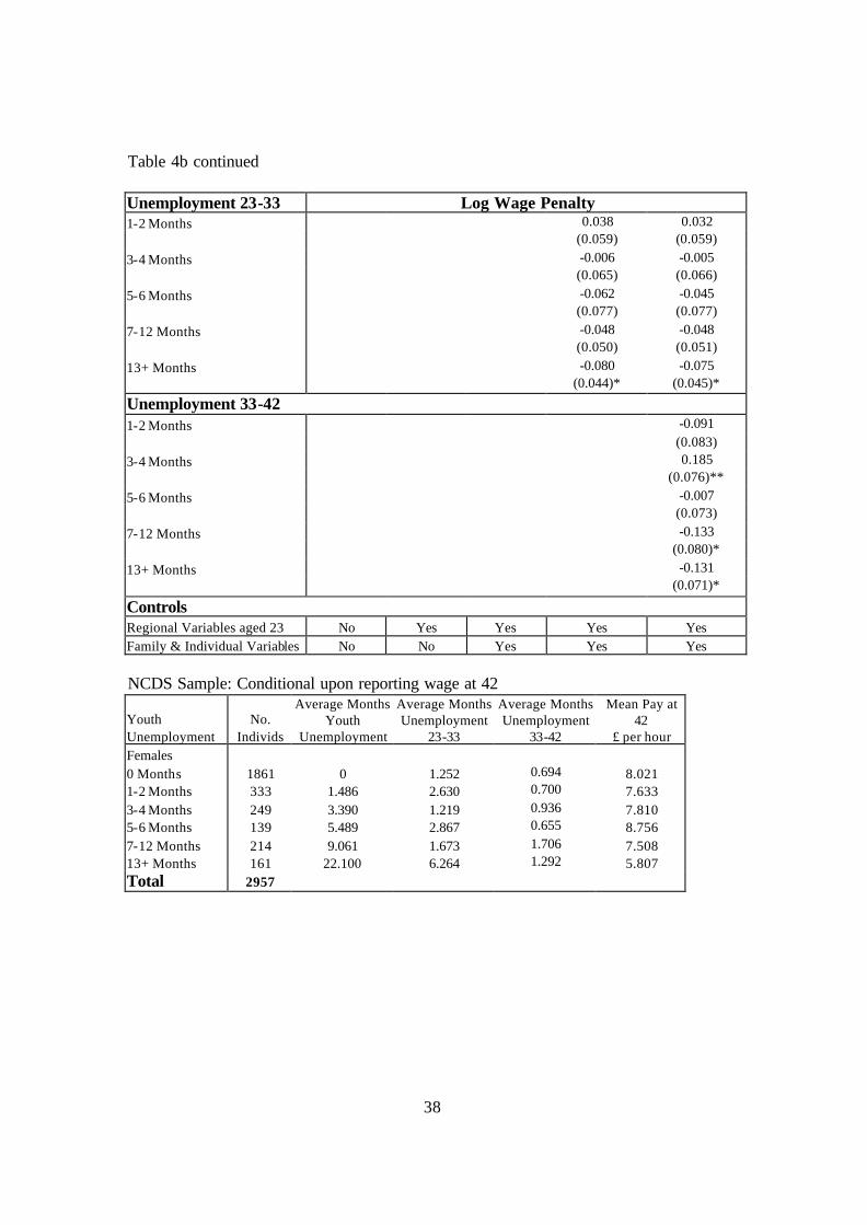
Again, it is informative to differentiate between the persistence of the wage penalty

derived through repeat exposure to unemployment and that which persists even with

continuous employment. In Tables 4a and b, columns IV and V display the scar at 42

controlling for unemployment exposure between ages 23 and 33 and then 33 to 42

additively. For men and women, long term youth unemployment of over 6 months

damages the wage at 42 even if they remain out of unemployment after the age of 23. The

magnitude of the permanent wage scar is modest at just 6-10% and the results remain

statistically significant. Intervening spells of unemployment are more important for men

than women and although repeat exposure after age 33 is important for wages,

conditioning on later unemployment exposure does not affect the magnitude of the wage

penalty associated with youth unemployment. That is, for men, once unemployment

experience between the ages of 23 and 33 is conditioned upon, further unemployment

20

experience is uncorrelated with youth unemployment patterns. As shown in Table 1 there

is a far more muted relationship between youth unemployment and that experienced after

age 33. Thus the persistence effect of unemployment dies out if a worker can avoid a

further spell for 10 years or so. However, they are still left with a wage scar. The direct

impact of recent unemployment on earnings is strong throughout such that over a year

worth of cumulated unemployment experiencing in the preceding 8 to 10 years

(depending upon the period) reduces wages by around 30% for men and 15-20% for

women.

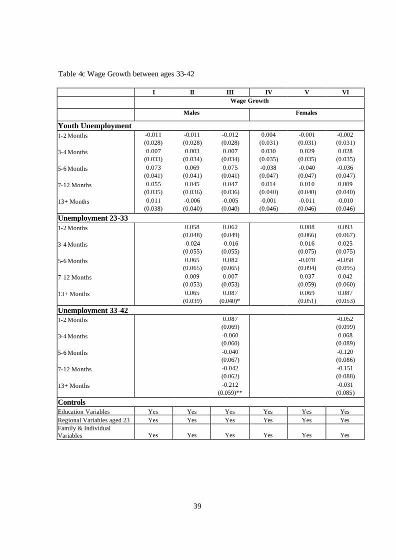
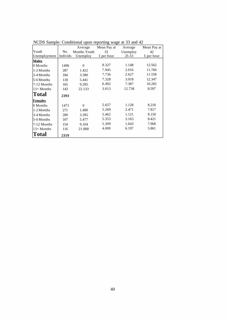
Table 4c analyses the wage growth prevalent between the age of 33 and 42. The sample

includes individuals reporting a wage at 33 and 42. Again this involves a change in

sample selection and we explore if this makes any difference by including a dummy

variable for not reporting a wage at 33 in the age 42 equation. The samples reporting both

wages have on average higher wages than those missing one or the other. Those reporting

a wage at 33 have wages at 42, which are 10% higher than for those that did not after

conditioning on other characteristics. Likewise, those reporting a wage at 42 had wages at

33 that were 7-8% higher than those that did not. There were no differences across gender

in these patterns. Hence the bias in growth appears small.

The coefficients reported in column I and IV show the relationship between wage growth

and youth unemployment, once education, region of residence, family and individual

characteristics have been controlled for, for men and women. The wage recovery is now

far less marked, with men experiencing 5+ months unemployment pre-23 showing

recovery of around 7%. The results for women are effectively zero. Columns II and V

further control for unemployment between 23-33 and columns III and VI control for

unemployment in the following decade. Evident from the table is that there is little

relative wage growth in the past two decades. Here it makes little difference whether

later unemployment is conditioned on. To summarise, the recovery of wages among

those experiencing 5+ months youth unemployment mainly occurs by age 33 unless it is

interrupted for some by repeat bursts of unemployment. Even so the recovery is partial

some twenty years later, suggesting a near permanent wage scar.

21

Further accounting for unobservable heterogeneity

Unobserved individual characteristics

In the results presented above the wage penalty associated with youth unemployment is

sharply reduced once education and region are conditioned on. However, further

conditioning on a wealth of individual ability and family background measures makes

only a modest further reduction in the relationship between youth unemployment and

wages. On one hand, this result might signify that we are capturing the major cross-

correlates between youth unemployment and wages leaving no residual bias from

unobserved heterogeneity and thus isolating the pure scarring effect. However, there may

be other variables which determine the hourly wage which are correlated with youth

unemployment and thus continue to cloud the observed scarring effect. The results

presented above show that wages at 23 do not differ significantly between those who go

on to experience more than 3 months further unemployment after age 23 and those who

have little or no further unemployment, after conditioning on observed characteristics.

Hence employers of cohort members at age 23 are not observing and rewarding some

ability component unobserved to the researcher, which is correlated with the revealed

future unemployment experience. This suggests that the large conditional wage penalties

at age 33, or indeed 42, associated with unemployment in the preceding decade were

unobservable to employers at 23 (or 33 for wages at 42). However, there may still be

concerns that youth unemployment experience reflects some unobserved ability factor

and that the persistent wage penalty reflects this unobserved ability rather than

unemployment per se.

Therefore we extended the current analysis by adopting an instrumental variables (IV)

approach to analyse the impact of youth unemployment upon the wage at 33. The

instrument is the local area (ward level) unemployment rate prevalent as the cohort

members can first enter the labour market at age 16. The intuition for the decision is that

at 16, the individual cohort members are unlikely to have chosen the area within which

they live. However the local unemployment rate certainly drives the labour market

experience of the individual; thus an exogenous source of variation in youth

22

unemployment experience can be captured by the instrument, allowing accurate

calculation of the true scarring effect. A strong instrument must drive wages whilst

remaining exogenous to the individual themselves. A likelihood ratio tests confirms the

strength of the instrument in driving youth unemployment: statistically the instrument is a

strong predictor of the endogenous variable.

To avoid the requirement of non-linear instruments, a linear model is adopted, where the

effect of one month of youth unemployment upon the natural log of the hourly wage

reported at age 33 is evaluated. In addition, there maybe a concern that some people will

not have left their home area by age 33 or have moved nearby. So we also condition on

ward level unemployment at age 33, to make sure our instrument is not capturing

persistence in residence. This disaggregated data on unemployment is not available at age

42 and hence we only focus on cohort members at age 33 for the IV estimation. Table 5

reports the results from an estimation controlling for education, region of residence,

family and individual effects. One month of unemployment will reduce a male

individual’s wage at 33 by 0.8% and will reduce a female individual’s wage at 33 by

0.7%, conditional on education level, measures of family background and ability and

ward level unemployment at age 33 from the 1991 Census. The application of the IV

technique does change the coefficients; the estimated impact of months of youth

unemployment upon the subsequent wage rises slightly, although the results are not

largely different from the OLS estimates. If heterogeneity was creating a bias in the

results and pushing up the perceived scarring effect from youth unemployment, the IV

technique should cause the impact of unemployment upon wages to fall. Even if the

instrument is capturing unobserved parental characteristics that have sorted families into

more deprived areas, as we condition on a lot of family and parental factors, then the bias

should still be reduced through the IV approach and the coefficient fall. Intergenerational

transmission produces far less than a complete replication across generations (see

Dearden et al. 1997).

One simple interpretation for the change could be that the inclusion of an instrument

creates ‘wobble’ in the coefficient on youth unemployment, which is never significantly

23

different from the un-instrumented coefficient. In other words, there is no economic

explanation for the observed movement of the coefficient. Alternatively an error could

lie in the assumption necessary for ease of calculation, of a linear relationship between

the hourly wage and months of youth unemployment. Although we explored this by

capping the months of unemployment at different levels between 25 and 50, the pattern

of results was unaffected. A third plausible explanation is that the instrument reflects

neighbourhood effects which influence youth’s unobserved characteristics and impact

upon both earnings and employment opportunities for youths. We cannot test for this

here, but given the assumption that the local employment conditions when youths first

enter the labour market affect youth’s early unemployment experiences in a way that is

exogenous to the unobserved characteristics of the individual, then the importance of the

results is that the instrumentation does not reduce the magnitude of the results –

suggesting that the wage penalty identified is accurate. Therefore we can conclude that

there are no substantive biases to our estimates of the scarring effects of youth

unemployment from unobserved heterogeneity.

6. Conclusion

There is a plethora of empirical evidence to suggest that a spell of unemployment harms

an individual’s labour market outcomes, both in terms of future employment prospects

and in terms of wages. We contribute to these studies by examining the consequence of

youth unemployment upon the cumulative wage experience up to twenty years later. We

look at the mechanisms by which youth unemployment translates into labour market

outcomes, in order to identify true potential for policy intervention. Our findings are that

youth unemployment imposes a sizeable wage scar upon both males and females at age

23 followed by substantial recovery over the next ten years, but only if the individual can

avoid further spells of unemployment after age 23. A modest residual wage scar of

around 8% persists up to twenty years later even for those who have no further

unemployment experience. Those with extensive youth unemployment are at higher risk

of further unemployment through to age 33 and this inhibits wage recovery. However

there was no further relationship between youth unemployment and unemployment

reported after age 33. The results suggest therefore that wages recovery slowly and

24

incompletely after a substantive bout of youth unemployment. Further, subsequent

exposure to unemployment retards this recovery process. So interventions to reduce the

exposure of young adults to substantive periods of unemployment could if successful

have substantial returns in terms of the individual’s lifetime earnings and could represent

a good investment.

25

BIBLIOGRAPHY

Abraham, K. G. and Farber, H. S. (1987). ‘Job duration, seniority and earnings’, American Economic Review, vol. 77(3), pp. 278-97. Abbring, J., van den Berg, G., Cautier, P. A., Lomwel, A. G. C., van Ours, J. C. and Rhum, C. J. (1998). ‘Displaced workers in the United States and the Netherlands’, in (P. Khun, eds) Losing Work, Moving On: International Perspectives on Worker Displacement. W. E. Upjohn Institute for Employment Research, forthcoming. Ackum, S. (1991). ‘Youth unemployment, labour market programs and subsequent earnings’, Scandinavian Journal of Economics, vol. 93(4), pp. 531-43. Albaek, K., van Audenrobe, M. and Browning, M. (1999). ‘Employment protection and the consequences for displaced workers: a comparison of Belgium and Denmark’, in (P. Khun, eds) Losing Work, Moving On: International Perspectives on Worker Displacement. W. E. Upjohn Institute for Employment Research, forthcoming. Altonji, J. G. and Shaktoko, R. A. (1987). ‘Do wages rise with job seniority?’, Review of Economic Studies, vol. 54(3), pp. 437-59. Altonji, J. G. and Williams, N. (1997). ‘Do wages rise with job seniority? A reassessment’, mimeo, paper presented at the Society of Labour Economists meeting held in Washington DC. Arulampalam, W. (2001). ‘Is unemployment really scarring? Effects of unemployment experiences on wages’, Economic Journal, vol. 111(475), pp. 585-606. Arulampalam, W., Booth, A. and Taylor, M. (2000). ‘Unemployment persistence’, Oxford Economic Papers, vol. 52, pp. 24-50. Arulampalam, W., Gregg, P. and Gregory, M. (2001). ‘Unemployment scarring’, Economic Journal, vol. 111(475), pp. 577-84. Ashenfelter, O. and Zimmerman, D. J. (1997). ‘Estimates of the return to schooling from sibling data: fathers, sons and brothers’, The Review of Economics and Statistics, vol. 79(1), pp. 1-9. Becker, G. S. (1975). Human Capital: A Theoretical and Empirical Analysis with Special Reference to Education, 2nd Edition, New York: NBER with Columbia University Press. Belzil, C. (1995). ‘Unemployment duration stigma and re-employment earnings’, Canadian Journal of Economics, vol. 28(3), pp. 568-85. Bender, S., Dustmann, C., Margolis, D. and Meghir, C. (1999). ‘Worker displacement in France and Germany’, IFS Working Paper, W99/14.

26

Borland, J. Gregg, P. Knight, J. And Wadsworth, J. (2002) They Get Knocked Down. Do they Get Up Again? Displaced Workers in Britain and Australia prepared for CILN conference on Displaced Workers, Burlington, Sept 1998. in Kuhn, P. (ed) Losing Work, Moving On: Worker Displacement in an International Context. Michigan, Upjohn Institute Davidson, R. and MacKinnon, J. G. (1993). Estimation and Inference in Econometrics, Oxford University Press. Dearden, L., Machin, S. and Reed, H. (1997), 'Intergenerational Mobility in Britain', Economic Journal, vol. 107(440), pp. 47-66. Dolton, P. and O’Neill, D. (1996). ‘Unemployment duration and the Restart effect: some experimental evidence’, Economic Journal, vol. 106(435), pp. 387-400. Farber, H. (1993). ‘The incidence and cost of job loss: 1982-91’, Brookings Papers on Economic Activity, pp. 73-132. Jacobson, L., LaLonde, R. and Sullivan, D. (1993). ‘Earnings losses of displaced workers’, American Economic Review, vol. 83, pp. 685-709. Gregg, P. (2001). ‘The impact of youth unemployment on adult employment in the NCDS’, Economic Journal, vol. 111(475), pp. 623-53. Gregg, P. and Machin, S. (2000). ‘Child development and success or failure in the youth labour market’ in (D. Blanchflower and R. Freemam, eds) Youth Unemployment and Joblessness in Advanced Countries, NBER Comparative Labour Market Series, Chicago: University of Chicago Press. Gregory, M. and Jukes, R. (2001). ‘Unemployment and subsequent earnings: estimating scarring among British men 1984-94’, Economic Journal, vol. 111(475), pp. 607-25. Heckman, J. and Borjas, G. (1980). ‘Does unemployment cause future unemployment? Definitions, questions and answers from a continuous time model of heterogeneity and state dependence’, Economica, vol. 47, pp. 247-83. Lockwood, B. (1991). ‘Information externalities in the labour market and the duration of unemployment’, Review of Economic Studies, vol. 58(4), pp. 733-53. Manning, A. (2000). ‘Pretty vacant: recruitment in low wage labour markets’, Oxford Bulletin of Economics and Statistics, vol. 62(SI), pp. 747-70. Manning, A. (2003) Monopsony in Motion, Princeton University Press, Princeton.

27

Mincer, J. (1974). Schooling, Experience and Earnings, New York: NBER with Columbia University Press. Narendranathan, W. and Elias, P. (1993). ‘Influences of past history on the incidence of youth unemployment: empirical findings for the UK’, Oxford Bulletin of Economics and Statistics, vol. 55(2), pp. 161-85. Nickell, S., Jones, P. and Quintini, G. (2002). ‘A picture of job insecurity facing British men’, Economic Journal vol. 112(476), pp. 1-27. Pissarides, C. , (1994). 'Search unemployment with on-the-job search', Review of Economic Studies, vol. 61, pp. 457-75. Rhum, C. J. (1991). ‘Are workers permanently scarred by job displacement?’, American Economic Review, vol. 81(1), pp. 319-24. Sianesi, B. and van Reenen, J. (2002). ‘The returns to education: a review of the empirical macro-economic literature’, IFS Working Papers, W02/05. Spence, M. (1973). ‘Job market signalling’, Quarterly Journal of Economics, vol. 87, no. 3, pp. 355-374. Stevens, A. H. (1997). ‘Persistent effects of job displacement: the importance of multiple job losses’, Journal of Labor Economics, vol. 15(1), pp. 165-88. Stewart , M. B. (2000). ‘The inter-related dynamics of unemployment and low pay’, University of Warwick, mimeo. Swaim, P. and Podgursky, M. (1991). ‘The distribution of economic losses among displaced workers: a replication’, Journal of Human Resources, vol. 26(4), Fall, pp. 742-55. Topel, R. (1991). ‘Specific capital, mobility and wages: wages rise with job seniority’, Journal of Political Economy, vol. 99(1), pp. 145-76.

28

Table 1 Summary of NCDS Sample

I II III IV V VI VII VIII

Youth Unemployment

16-23

No. Indivds

% of Sample

Average Months Youth

Unemployment 16-23

Mean Pay at 23 £ per hour

(2000 prices)

Average Months Unemployment

23-33

Mean Pay at 33

£ per hour (2000 prices)

Average Months

Unemployment 33-42

Mean Pay at 42

£ per hour (2000 prices)

Men

0 months 2607 58.6 0 6.400 1.450 10.500 1.160 12.386 1-2 months 539 12.1 1.430 6.190 3.023 9.823 1.581 12.195 3-4 months 364 8.2 3.374 5.938 2.984 9.649 3.280 11.728 5-6 months 231 5.2 5.472 5.660 4.627 9.045 1.814 11.778 7-12 months 342 7.7 9.190 5.553 7.285 8.090 4.368 9.989 13+ months 366 8.2 25.680 4.726 21.745 7.132 10.150 8.461 Total 4449 100

Women

0 months 2769 61.1 0 5.680 1.315 6.841 0.786 8.021 1-2 months 516 11.4 1.483 5.555 2.548 6.844 0.831 7.633 3-4 months 384 8.5 3.401 5.134 1.829 6.658 0.766 7.810 5-6 months 215 4.7 5.484 5.000 3.352 6.469 0.898 8.756 7-12 months 335 7.4 9.167 4.795 2.896 6.299 2.284 7.508 13+ months 314 6.9 23.815 4.100 8.207 4.911 2.025 5.807 Total 4533 100

29

Table 2a Dependent Variable is Log Wage Penalty aged 23 for Males I II III

Youth Unemployment Log Wage Penalty

1-2 Months -0.033 -0.021 -0.016 (0.020) (0.020) (0.020) 3-4 Months -0.055 -0.041 -0.042 (0.025)** (0.024)* (0.025)* 5-6 Months -0.126 -0.112 -0.105 (0.031)** (0.031)** (0.031)** 7-12 Months -0.131 -0.100 -0.100 (0.029)** (0.028)** (0.029)** 13+ Months -0.296 -0.242 -0.232 (0.034)** (0.034)** (0.034)**

Education Variables

Lower vocational 0.100 0.107 Qualifications (0.063) (0.063)* Lower academic 0.035 0.023 (0.049) (0.049) Intermediate Vocational 0.095 0.080 (0.045)** (0.045)* O’Level or equivalent 0.104 0.091 (0.019)** (0.021)** Higher Vocational 0.153 0.139 (0.021)** (0.023)** A’Level or equivalent 0.174 0.154 (0.031)** (0.034)** Level 5 vocational 0.178 0.161 (0.026)** (0.028)** Degree or equivalent 0.126 0.105 (0.025)** (0.030)**

Controls Regional Variables aged 234 No Yes Yes Family & Individual Variables No No Yes

NCDS Sample: Conditional upon reporting wage at 23

Youth Unemployment No. Individs % of

Sample Mean Pay at 23

£ per hour (2000 prices) Average Months Youth

Unemployment Males 0 Months 2263 6.400 0 1-2 Months 449 6.190 1.425 3-4 Months 286 5.940 3.392 5-6 Months 169 5.660 5.420 7-12 Months 207 5.553 9.048 13+ Months 146 4.726 23.274 Total 3520

4 Full regression results are available from the authors.

30

Table 2b Dependent Variable is Log Wage Penalty aged 23 for Females I II III

Youth Unemployment Log Wage Penalty

1-2 Months -0.029 -0.039 -0.036 (0.024) (0.023)* (0.023) 3-4 Months -0.103 -0.119 -0.116 (0.029)** (0.027)** (0.027)** 5-6 Months -0.133 -0.129 -0.127 (0.038)** (0.036)** (0.036)** 7-12 Months -0.154 -0.146 -0.125 (0.033)** (0.031)** (0.031)** 13+ Months -0.335 -0.221 -0.192 (0.042)** (0.040)** (0.040)** Education Variables

Lower vocational 0.028 -0.012 Qualifications (0.052) (0.052) Lowe r academic 0.024 -0.020 (0.068) (0.067) Intermediate Vocational -0.018 -0.024 (0.088) (0.087) O’Level or equivalent 0.141 0.063 (0.021)** (0.022)** Higher Vocational 0.231 0.136 (0.031)** (0.033)** A’Level or equivalent 0.310 0.199 (0.034)** (0.037)** Level 5 vocational 0.351 0.261 (0.027)** (0.029)** Degree or equivalent 0.425 0.308 (0.027)** (0.032)** Controls Regional Variables aged 23 No Yes Yes Family & Individual Variables No No Yes NCDS Sample: Conditional upon reporting wage at 23

Youth Unemployment No. Individs Mean Pay at 23

£ per hour (2000 prices) Average Months Youth

Unemployment Females 0 Months 1942 5.680 0 1-2 Months 351 5.555 1.479 3-4 Months 242 5.134 3.397 5-6 Months 127 5.000 5.496 7-12 Months 174 4.795 9.109 13+ Months 103 4.000 20.990 Total 2939

31

Table 3a Dependent Variable is Log Wage Penalty aged 33 for Males I II III IV

Youth Unemployment Log Wage Penalty

1-2 Months -0.075 -0.030 -0.026 -0.014 (0.024)** (0.021) (0.021) (0.021) 3-4 Months -0.098 -0.089 -0.090 -0.070 (0.029)** (0.025)** (0.025)** (0.025)** 5-6 Months -0.136 -0.113 -0.106 -0.073 (0.035)** (0.031)** (0.030)** (0.030)** 7-12 Months -0.252 -0.160 -0.154 -0.106 (0.030)** (0.027)** (0.026)** (0.026)** 13+ Months -0.424 -0.252 -0.231 -0.133 (0.030)** (0.027)** (0.027)** (0.028)**

Education Variables Lower vocational 0.231 0.207 0.193 qualifications (0.060)** (0.059)** (0.058)** Lower academic 0.117 0.084 0.082 (0.051)** (0.051)* (0.050)* Intermediate Vocational 0.160 0.115 0.110 (0.051)** (0.051)** (0.050)** O’Level or equivalent 0.227 0.156 0.151 (0.020)** (0.021)** (0.021)** Higher Vocational 0.277 0.199 0.190 (0.023)** (0.024)** (0.023)** A’Level or equivalent 0.489 0.357 0.350 (0.031)** (0.034)** (0.033)** Level 5 vocational 0.448 0.347 0.333 (0.027)** (0.029)** (0.028)** Degree or equivalent 0.603 0.457 0.450 (0.025)** (0.030)** (0.029)**

Unemployment 23-33

1-2 Months -0.031 (0.036) 3-4 Months -0.185 (0.041)** 5-6 Months -0.192 (0.048)** 7-12 Months -0.158 (0.036)** 13+ Months -0.297 (0.027)**

Controls

Regional Variables aged 23 No Yes Yes Yes Family & Individual Variables No No Yes Yes

32

NCDS Sample of Males: Conditional upon reporting wage at 33

Youth Unemployment No. Individs

Average Months Youth

Unemployment

Mean Pay at 33

£ per hour (2000 prices)

Average Unemployment

23-33

Males 0 Months 1924 0 10.500 1.413 1-2 Months 400 1.430 9.823 2.865 3-4 Months 267 3.371 9.649 3.187 5-6 Months 172 5.459 9.045 4.430 7-12 Months 240 9.217 8.100 7.225 13+ Months 245 25.233 7.132 18.775 Total 3248

33

Table 3b Dependent Variable is Log Wage Penalty aged 33 for Females I II III IV

Youth Unemployment Log Wage Penalty

1-2 Months -0.025 -0.034 -0.031 -0.023 (0.029) (0.025) (0.024) (0.024) 3-4 Months -0.049 -0.085 -0.083 -0.081 (0.033) (0.029)** (0.028)** (0.028)** 5-6 Months -0.099 -0.059 -0.060 -0.050 (0.044)** (0.038) (0.037) (0.037) 7-12 Months -0.121 -0.086 -0.077 -0.067 (0.036)** (0.031)** (0.031)** (0.031)** 13+ Months -0.350 -0.185 -0.166 -0.141 (0.038)** (0.033)** (0.033)** (0.033)** Education Variables

Lower vocational 0.203 0.160 0.162 qualifications (0.056)** (0.056)** (0.056)** Lower academic 0.223 0.176 0.180 (0.075)** (0.075)* (0.074)* Intermediate Vocational -0.146 -0.128 -0.144 (0.104) (0.103) (0.103) O’Level or equivalent 0.199 0.131 0.129 (0.020)** (0.022)** (0.022)** Higher Vocational 0.394 0.311 0.302 (0.035)** (0.037)** (0.037)** A’Level or equivalent 0.573 0.451 0.443 (0.038)** (0.041)** (0.041)** Level 5 vocational 0.626 0.544 0.538 (0.029)** (0.031)** (0.031)** Degree or equivalent 0.785 0.657 0.648 (0.029)** (0.034)** (0.034)** Unemployment 23-33

1-2 Months 0.037 (0.052) 3-4 Months -0.073 (0.058) 5-6 Months 0.002 (0.067) 7-12 Months -0.098 (0.045)* 13+ Months -0.186 (0.038)**

Controls

Regional Variables aged 23 No Yes Yes Yes Family & Individual Variables No No Yes Yes

34

NCDS Sample of Females: Conditional upon reporting wage at 33

Youth Unemployment No. Individs

Average Months Youth

Unemployment

Mean Pay at 33

£ per hour

Average Unemployment

23-33 Females 0 Months 2016 0 7.186 1.112 1-2 Months 394 1.464 6.844 2.595 3-4 Months 282 3.401 6.658 1.487 5-6 Months 152 5.493 6.469 4.041 7-12 Months 233 9.227 6.299 2.516 13+ Months 209 22.321 4.911 7.047 Total 3286

Table 3c Dependent Variable is Wage Growth between ages 23-33

I II III IV V VI

Wage Growth

Males Females

Youth Unemployment

1-2 Months 0.023 0.035 0.041 -0.038 -0.032 -0.033 (0.026) (0.026) (0.026) (0.033) (0.033) (0.033) 3-4 Months -0.015 -0.001 -0.003 -0.010 -0.009 -0.019 (0.032) (0.032) (0.032) (0.039) (0.039) (0.039) 5-6 Months 0.044 0.061 0.063 0.088 0.090 0.083 (0.041) (0.041) (0.040) (0.053)* (0.053)* (0.053) 7-12 Months -0.042 -0.025 -0.029 0.053 0.065 0.063 (0.039) (0.038) (0.038) (0.045) (0.045) (0.045) 13+ Months 0.048 0.082 0.081 0.035 0.056 0.053 (0.045) (0.045)* (0.044)* (0.059) (0.060) (0.059) Unemployment 23-33

1-2 Months 0.050 0.046 0.114 0.113 (0.049) (0.049) (0.075) (0.074) 3-4 Months -0.174 -0.182 -0.092 -0.093 (0.059)** (0.059)** (0.074) (0.073) 5-6 Months 0.027 0.024 -0.124 -0.128 (0.067) (0.067) (0.093) (0.093) 7-12 Months -0.173 -0.167 -0.032 -0.022 (0.051)** (0.051)** (0.061) (0.061) 13+ Months -0.260 -0.260 -0.178 -0.185 (0.042)** (0.042)** (0.058)** (0.058)** Educational Upgrade 0.108 0.153

(0.023)** (0.033)** Controls

Education Variables Yes Yes Yes Yes Yes Yes Regional Variables aged 23 Yes Yes Yes Yes Yes Yes Family & Individual Variables Yes Yes Yes Yes Yes Yes

35

Table 4a Dependent Variable is Log Wage at age 42 for Males I II III IV V

Youth Unemployment Log Wage Penalty

1-2 Months -0.076 -0.041 -0.039 -0.031 -0.029 (0.031)** (0.028) (0.028) (0.028) (0.028) 3-4 Months -0.046 -0.055 -0.051 -0.037 -0.026 (0.037) (0.034)* (0.034) (0.034) (0.033) 5-6 Months -0.038 -0.020 -0.006 0.016 0.020 (0.046) (0.042) (0.042) (0.042) (0.042) 7-12 Months -0.184 -0.125 -0.118 -0.078 -0.070 (0.038)** (0.035)** (0.035)** (0.035)** (0.035)** 13+ Months -0.315 -0.182 -0.154 -0.094 -0.078 (0.041)** (0.038)** (0.038)** (0.039)** (0.039)**

Education Variables

Lower vocational 0.171 0.151 0.157 0.143 qualifications (0.084)** (0.084)* (0.083)* (0.083)* Lower academic 0.124 0.097 0.099 0.087 (0.070)* (0.070) (0.069) (0.069) Intermediate Vocational 0.071 0.040 0.048 0.028 (0.065) (0.065) (0.065) (0.064) O’Level or equivalent 0.230 0.163 0.164 0.156 (0.027)** (0.029)** (0.028)** (0.028)** Higher Vocational 0.280 0.207 0.207 0.198 (0.030)** (0.032)** (0.032)** (0.032)** A’Level or equivalent 0.572 0.453 0.451 0.436 (0.041)** (0.045)** (0.044)** (0.044)** Level 5 vocational 0.404 0.308 0.300 0.287 (0.036)** (0.038)** (0.038)** (0.038)** Degree or equivalent 0.644 0.504 0.505 0.486 (0.033)** (0.039)** (0.039)** (0.039)**

36

Table 4a continued Unemployment 23-33 Log Wage Penalty 1-2 Months 0.002 0.028 (0.048) (0.049) 3-4 Months -0.155 -0.136 (0.056)** (0.056)** 5-6 Months -0.148 -0.108 (0.063)** (0.064)* 7-12 Months -0.154 -0.133 (0.051)** (0.051)** 13+ Months -0.195 -0.145 (0.039)** (0.040)**

Unemployment 33-42

1-2 Months -0.052 (0.067) 3-4 Months -0.141 (0.060)** 5-6 Months -0.051 (0.066) 7-12 Months -0.218 (0.060)** 13+ Months -0.270 (0.053)**

Controls

Regional Variables aged 23 No Yes Yes Yes Yes Family & Individual Variables No No Yes Yes Yes NCDS Sample: Conditional upon reporting wage at 42

Youth Unemployment

No. Individs

Average Months Youth

Unemployment

Average Months Unemployment

23-33

Average Months Unemployment

33-42

Mean Pay at 42

£ per hour Males 0 Months 1722 0 1.221 0.963 12.386 1-2 Months 340 1.424 2.379 1.182 12.195 3-4 Months 226 3.385 2.802 2.960 11.728 5-6 Months 137 5.460 2.925 1.036 11.778 7-12 Months 215 9.107 7.427 3.214 9.990 13+ Months 182 22.429 16.277 6.148 8.461 Total 2822

37

Table 4b Dependent Variable is Log Wage at aged 42 for Females I II III IV V

Youth Unemployment Log Wage Penalty

1-2 Months -0.039 -0.044 -0.040 -0.038 -0.038 (0.031) (0.027) (0.027) (0.027) (0.027) 3-4 Months -0.004 -0.032 -0.027 -0.027 -0.025 (0.035) (0.031) (0.031) (0.031) (0.031) 5-6 Months -0.026 -0.018 -0.018 -0.013 -0.011 (0.045) (0.040) (0.040) (0.040) (0.040) 7-12 Months -0.068 -0.058 -0.063 -0.062 -0.059 (0.037)* (0.033)* (0.033)* (0.033)* (0.033)* 13+ Months -0.252 -0.114 -0.116 -0.107 -0.101 (0.042)** (0.038)** (0.038)** (0.039)** (0.039)**

Education Variables

Lower vocational 0.077 0.044 0.046 0.039 qualifications (0.061) (0.062) (0.062) (0.062) Lower academic -0.002 -0.048 -0.047 -0.050 (0.087) (0.087) (0.087) (0.087) Intermediate Vocational 0.016 0.016 0.015 0.014 (0.107) (0.106) (0.106) (0.106) O’Level or equivalent 0.177 0.134 0.133 0.133 (0.022)** (0.024)** (0.024)** (0.024)** Higher Vocational 0.321 0.267 0.263 0.261 (0.038)** (0.040)** (0.040)** (0.040)** A’Level or equivalent 0.494 0.418 0.414 0.415 (0.040)** (0.044)** (0.044)** (0.043)** Level 5 vocational 0.571 0.519 0.516 0.515 (0.031)** (0.033)** (0.033)** (0.033)** Degree or equivalent 0.729 0.643 0.639 0.638 (0.032)** (0.037)** (0.037)** (0.037)**

38

Table 4b continued Unemployment 23-33 Log Wage Penalty 1-2 Months 0.038 0.032 (0.059) (0.059) 3-4 Months -0.006 -0.005 (0.065) (0.066) 5-6 Months -0.062 -0.045 (0.077) (0.077) 7-12 Months -0.048 -0.048 (0.050) (0.051) 13+ Months -0.080 -0.075 (0.044)* (0.045)*

Unemployment 33-42

1-2 Months -0.091 (0.083) 3-4 Months 0.185 (0.076)** 5-6 Months -0.007 (0.073) 7-12 Months -0.133 (0.080)* 13+ Months -0.131 (0.071)*

Controls

Regional Variables aged 23 No Yes Yes Yes Yes Family & Individual Variables No No Yes Yes Yes NCDS Sample: Conditional upon reporting wage at 42

Youth Unemployment

No. Individs

Average Months Youth

Unemployment

Average Months Unemployment

23-33

Average Months Unemployment

33-42

Mean Pay at 42

£ per hour Females 0 Months 1861 0 1.252 0.694 8.021 1-2 Months 333 1.486 2.630 0.700 7.633 3-4 Months 249 3.390 1.219 0.936 7.810 5-6 Months 139 5.489 2.867 0.655 8.756 7-12 Months 214 9.061 1.673 1.706 7.508 13+ Months 161 22.100 6.264 1.292 5.807 Total 2957

39

Table 4c Wage Growth between ages 33-42 I II III IV V VI

Wage Growth

Males Females

Youth Unemployment 1-2 Months -0.011 -0.011 -0.012 0.004 -0.001 -0.002 (0.028) (0.028) (0.028) (0.031) (0.031) (0.031) 3-4 Months 0.007 0.003 0.007 0.030 0.029 0.028 (0.033) (0.034) (0.034) (0.035) (0.035) (0.035) 5-6 Months 0.073 0.069 0.075 -0.038 -0.040 -0.036 (0.041) (0.041) (0.041) (0.047) (0.047) (0.047) 7-12 Months 0.055 0.045 0.047 0.014 0.010 0.009 (0.035) (0.036) (0.036) (0.040) (0.040) (0.040) 13+ Months 0.011 -0.006 -0.005 -0.001 -0.011 -0.010 (0.038) (0.040) (0.040) (0.046) (0.046) (0.046)

Unemployment 23-33 1-2 Months 0.058 0.062 0.088 0.093 (0.048) (0.049) (0.066) (0.067) 3-4 Months -0.024 -0.016 0.016 0.025 (0.055) (0.055) (0.075) (0.075) 5-6 Months 0.065 0.082 -0.078 -0.058 (0.065) (0.065) (0.094) (0.095) 7-12 Months 0.009 0.007 0.037 0.042 (0.053) (0.053) (0.059) (0.060) 13+ Months 0.065 0.087 0.069 0.087 (0.039) (0.040)* (0.051) (0.053)

Unemployment 33-42 1-2 Months 0.087 -0.052 (0.069) (0.099) 3-4 Months -0.060 0.068 (0.060) (0.089) 5-6 Months -0.040 -0.120 (0.067) (0.086) 7-12 Months -0.042 -0.151 (0.062) (0.088) 13+ Months -0.212 -0.031 (0.059)** (0.085)

Controls Education Variables Yes Yes Yes Yes Yes Yes Regional Variables aged 23 Yes Yes Yes Yes Yes Yes Family & Individual Variables Yes Yes Yes Yes Yes Yes

40

NCDS Sample: Conditional upon reporting wage at 33 and 42

Youth Unemployment

No. Individs

Average Months Youth

Unemploy

Mean Pay at 33

£ per hour

Average Unemploy

23-33

Mean Pay at 42

£ per hour Males 0 Months 1496 0 8.327 1.148 12.562 1-2 Months 287 1.422 7.945 2.016 11.760 3-4 Months 184 3.380 7.736 2.627 11.558 5-6 Months 118 5.441 7.328 3.018 12.347 7-12 Months 165 9.285 6.492 7.387 10.282 13+ Months 143 22.133 3.013 12.738 8.597

Total 2393

Females 0 Months 1471 0 5.657 1.128 8.218 1-2 Months 271 1.480 5.269 2.471 7.817 3-4 Months 200 3.395 5.462 1.121 8.150 5-6 Months 107 5.477 5.353 3.163 8.421 7-12 Months 154 9.104 5.309 1.643 7.968 13+ Months 116 21.888 4.000 6.197 5.861

Total 2319

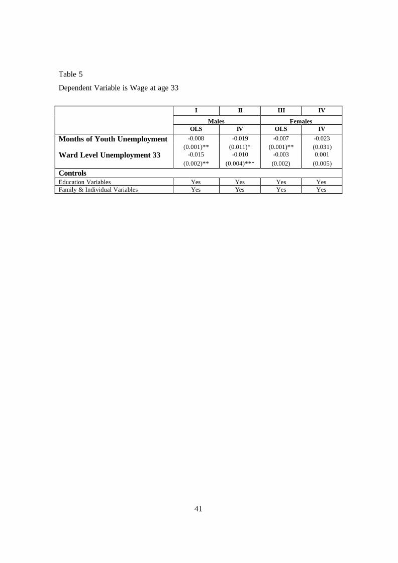
41

Table 5

Dependent Variable is Wage at age 33

I II III IV

Males Females OLS IV OLS IV

Months of Youth Unemployment -0.008 -0.019 -0.007 -0.023 (0.001)** (0.011)* (0.001)** (0.031) Ward Level Unemployment 33 -0.015 -0.010 -0.003 0.001 (0.002)** (0.004)*** (0.002) (0.005)

Controls Education Variables Yes Yes Yes Yes Family & Individual Variables Yes Yes Yes Yes

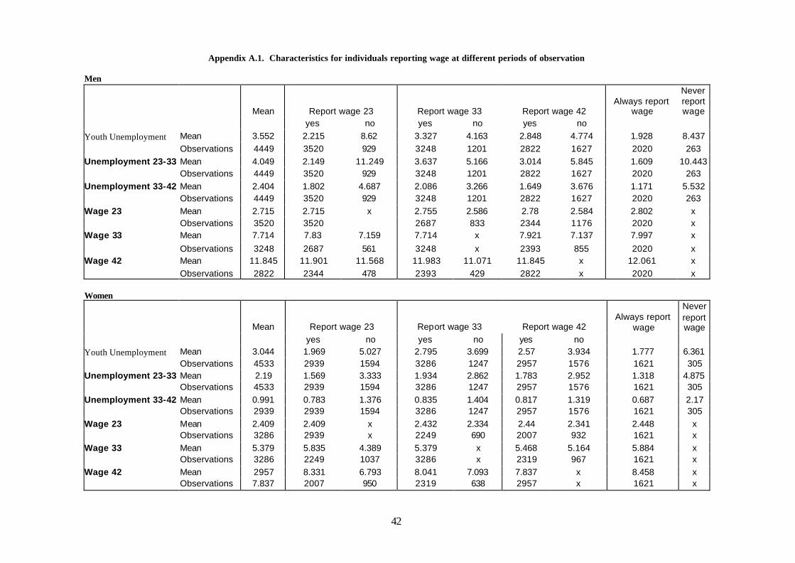
42

Appendix A.1. Characteristics for individuals reporting wage at different periods of observation

Men

Mean Report wage 23 Report wage 33 Report wage 42 Always report

wage

Never report wage

yes no yes no yes no Youth Unemployment Mean 3.552 2.215 8.62 3.327 4.163 2.848 4.774 1.928 8.437 Observations 4449 3520 929 3248 1201 2822 1627 2020 263 Unemployment 23-33 Mean 4.049 2.149 11.249 3.637 5.166 3.014 5.845 1.609 10.443 Observations 4449 3520 929 3248 1201 2822 1627 2020 263 Unemployment 33-42 Mean 2.404 1.802 4.687 2.086 3.266 1.649 3.676 1.171 5.532 Observations 4449 3520 929 3248 1201 2822 1627 2020 263 Wage 23 Mean 2.715 2.715 x 2.755 2.586 2.78 2.584 2.802 x Observations 3520 3520 2687 833 2344 1176 2020 x Wage 33 Mean 7.714 7.83 7.159 7.714 x 7.921 7.137 7.997 x Observations 3248 2687 561 3248 x 2393 855 2020 x Wage 42 Mean 11.845 11.901 11.568 11.983 11.071 11.845 x 12.061 x Observations 2822 2344 478 2393 429 2822 x 2020 x

Women

Mean Report wage 23 Report wage 33 Report wage 42 Always report

wage

Never report wage

yes no yes no yes no Youth Unemployment Mean 3.044 1.969 5.027 2.795 3.699 2.57 3.934 1.777 6.361 Observations 4533 2939 1594 3286 1247 2957 1576 1621 305 Unemployment 23-33 Mean 2.19 1.569 3.333 1.934 2.862 1.783 2.952 1.318 4.875 Observations 4533 2939 1594 3286 1247 2957 1576 1621 305 Unemployment 33-42 Mean 0.991 0.783 1.376 0.835 1.404 0.817 1.319 0.687 2.17 Observations 2939 2939 1594 3286 1247 2957 1576 1621 305 Wage 23 Mean 2.409 2.409 x 2.432 2.334 2.44 2.341 2.448 x Observations 3286 2939 x 2249 690 2007 932 1621 x Wage 33 Mean 5.379 5.835 4.389 5.379 x 5.468 5.164 5.884 x Observations 3286 2249 1037 3286 x 2319 967 1621 x Wage 42 Mean 2957 8.331 6.793 8.041 7.093 7.837 x 8.458 x Observations 7.837 2007 950 2319 638 2957 x 1621 x

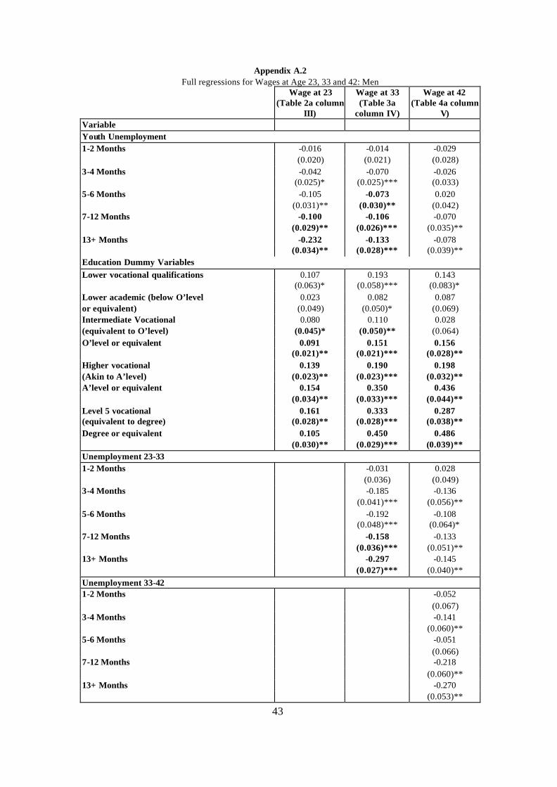
43

Appendix A.2 Full regressions for Wages at Age 23, 33 and 42: Men

Wage at 23 (Table 2a column

III)

Wage at 33 (Table 3a

column IV)

Wage at 42 (Table 4a column

V) Variable Youth Unemployment 1-2 Months -0.016 -0.014 -0.029

(0.020) (0.021) (0.028) 3-4 Months -0.042 -0.070 -0.026

(0.025)* (0.025)*** (0.033) 5-6 Months -0.105 -0.073 0.020

(0.031)** (0.030)** (0.042) 7-12 Months -0.100 -0.106 -0.070

(0.029)** (0.026)*** (0.035)** 13+ Months -0.232 -0.133 -0.078

(0.034)** (0.028)*** (0.039)** Education Dummy Variables Lower vocational qualifications 0.107 0.193 0.143

(0.063)* (0.058)*** (0.083)* Lower academic (below O’level 0.023 0.082 0.087 or equivalent) (0.049) (0.050)* (0.069) Intermediate Vocational 0.080 0.110 0.028 (equivalent to O’level) (0.045)* (0.050)** (0.064) O’level or equivalent 0.091 0.151 0.156

(0.021)** (0.021)*** (0.028)** Higher vocational 0.139 0.190 0.198 (Akin to A’level) (0.023)** (0.023)*** (0.032)** A’level or equivalent 0.154 0.350 0.436

(0.034)** (0.033)*** (0.044)** Level 5 vocational 0.161 0.333 0.287 (equivalent to degree) (0.028)** (0.028)*** (0.038)** Degree or equivalent 0.105 0.450 0.486 (0.030)** (0.029)*** (0.039)** Unemployment 23-33 1-2 Months -0.031 0.028

(0.036) (0.049) 3-4 Months -0.185 -0.136

(0.041)*** (0.056)** 5-6 Months -0.192 -0.108

(0.048)*** (0.064)* 7-12 Months -0.158 -0.133

(0.036)*** (0.051)** 13+ Months -0.297 -0.145 (0.027)*** (0.040)** Unemployment 33-42 1-2 Months -0.052

(0.067) 3-4 Months -0.141

(0.060)** 5-6 Months -0.051

(0.066) 7-12 Months -0.218

(0.060)** 13+ Months -0.270 (0.053)**

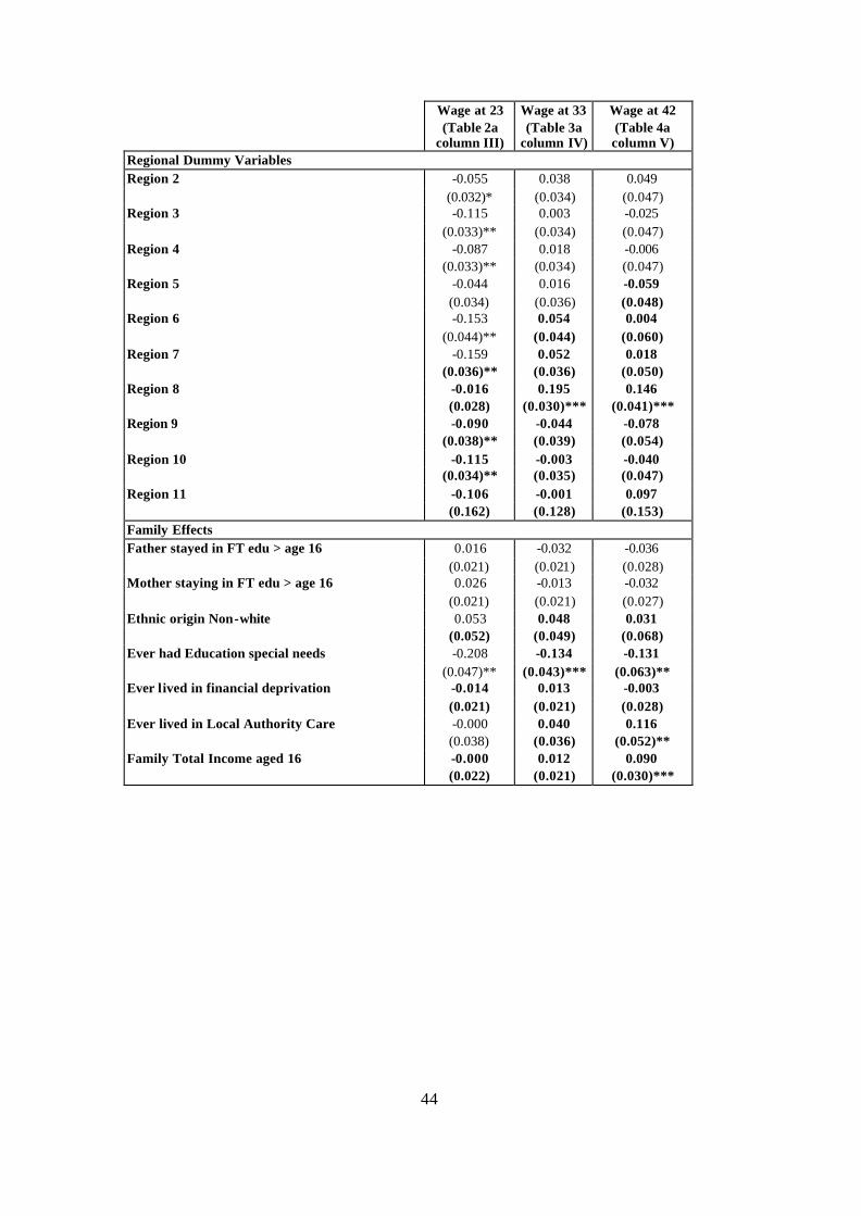
44

Wage at 23 (Table 2a

column III)

Wage at 33 (Table 3a

column IV)

Wage at 42 (Table 4a column V)

Regional Dummy Variables Region 2 -0.055 0.038 0.049

(0.032)* (0.034) (0.047) Region 3 -0.115 0.003 -0.025

(0.033)** (0.034) (0.047) Region 4 -0.087 0.018 -0.006

(0.033)** (0.034) (0.047) Region 5 -0.044 0.016 -0.059

(0.034) (0.036) (0.048) Region 6 -0.153 0.054 0.004

(0.044)** (0.044) (0.060) Region 7 -0.159 0.052 0.018

(0.036)** (0.036) (0.050) Region 8 -0.016 0.195 0.146

(0.028) (0.030)*** (0.041)*** Region 9 -0.090 -0.044 -0.078

(0.038)** (0.039) (0.054) Region 10 -0.115 -0.003 -0.040

(0.034)** (0.035) (0.047) Region 11 -0.106 -0.001 0.097

(0.162) (0.128) (0.153) Family Effects Father stayed in FT edu > age 16 0.016 -0.032 -0.036

(0.021) (0.021) (0.028) Mother staying in FT edu > age 16 0.026 -0.013 -0.032

(0.021) (0.021) (0.027) Ethnic origin Non-white 0.053 0.048 0.031

(0.052) (0.049) (0.068) Ever had Education special needs -0.208 -0.134 -0.131

(0.047)** (0.043)*** (0.063)** Ever lived in financial deprivation -0.014 0.013 -0.003

(0.021) (0.021) (0.028) Ever lived in Local Authority Care -0.000 0.040 0.116

(0.038) (0.036) (0.052)** Family Total Income aged 16 -0.000 0.012 0.090

(0.022) (0.021) (0.030)***

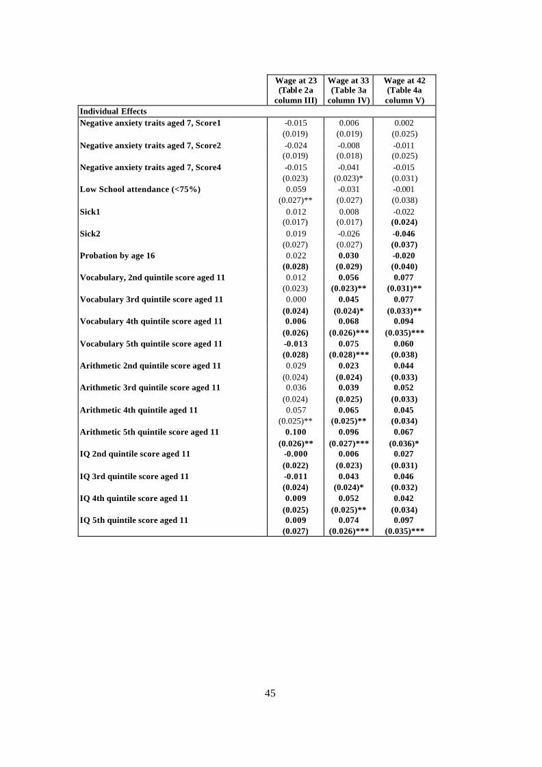
45

Wage at 23

(Table 2a column III)

Wage at 33 (Table 3a

column IV)

Wage at 42 (Table 4a column V)

Individual Effects Negative anxiety traits aged 7, Score1 -0.015 0.006 0.002

(0.019) (0.019) (0.025) Negative anxiety traits aged 7, Score2 -0.024 -0.008 -0.011

(0.019) (0.018) (0.025) Negative anxiety traits aged 7, Score4 -0.015 -0.041 -0.015

(0.023) (0.023)* (0.031) Low School attendance (<75%) 0.059 -0.031 -0.001

(0.027)** (0.027) (0.038) Sick1 0.012 0.008 -0.022

(0.017) (0.017) (0.024) Sick2 0.019 -0.026 -0.046

(0.027) (0.027) (0.037) Probation by age 16 0.022 0.030 -0.020

(0.028) (0.029) (0.040) Vocabulary, 2nd quintile score aged 11 0.012 0.056 0.077

(0.023) (0.023)** (0.031)** Vocabulary 3rd quintile score aged 11 0.000 0.045 0.077

(0.024) (0.024)* (0.033)** Vocabulary 4th quintile score aged 11 0.006 0.068 0.094

(0.026) (0.026)*** (0.035)*** Vocabulary 5th quintile score aged 11 -0.013 0.075 0.060

(0.028) (0.028)*** (0.038) Arithmetic 2nd quintile score aged 11 0.029 0.023 0.044

(0.024) (0.024) (0.033) Arithmetic 3rd quintile score aged 11 0.036 0.039 0.052

(0.024) (0.025) (0.033) Arithmetic 4th quintile aged 11 0.057 0.065 0.045

(0.025)** (0.025)** (0.034) Arithmetic 5th quintile score aged 11 0.100 0.096 0.067

(0.026)** (0.027)*** (0.036)* IQ 2nd quintile score aged 11 -0.000 0.006 0.027

(0.022) (0.023) (0.031) IQ 3rd quintile score aged 11 -0.011 0.043 0.046

(0.024) (0.024)* (0.032) IQ 4th quintile score aged 11 0.009 0.052 0.042

(0.025) (0.025)** (0.034) IQ 5th quintile score aged 11 0.009 0.074 0.097

(0.027) (0.026)*** (0.035)***

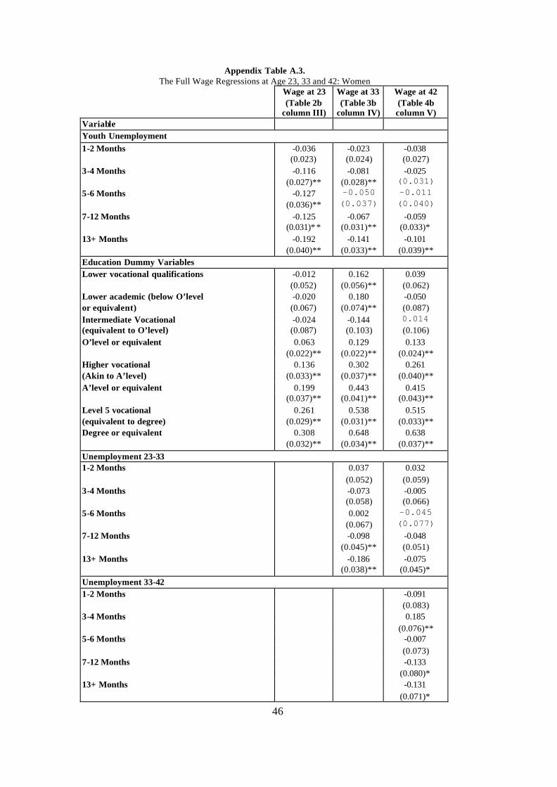
46

Appendix Table A.3. The Full Wage Regressions at Age 23, 33 and 42: Women

Wage at 23 (Table 2b

column III)

Wage at 33 (Table 3b

column IV)

Wage at 42 (Table 4b column V)

Variable Youth Unemployment 1-2 Months -0.036 -0.023 -0.038

(0.023) (0.024) (0.027) 3-4 Months -0.116 -0.081 -0.025

(0.027)** (0.028)** (0.031) 5-6 Months -0.127 -0.050 -0.011

(0.036)** (0.037) (0.040) 7-12 Months -0.125 -0.067 -0.059

(0.031)* * (0.031)** (0.033)* 13+ Months -0.192 -0.141 -0.101

(0.040)** (0.033)** (0.039)** Education Dummy Variables Lower vocational qualifications -0.012 0.162 0.039

(0.052) (0.056)** (0.062) Lower academic (below O’level -0.020 0.180 -0.050 or equivalent) (0.067) (0.074)** (0.087) Intermediate Vocational -0.024 -0.144 0.014 (equivalent to O’level) (0.087) (0.103) (0.106) O’level or equivalent 0.063 0.129 0.133

(0.022)** (0.022)** (0.024)** Higher vocational 0.136 0.302 0.261 (Akin to A’level) (0.033)** (0.037)** (0.040)** A’level or equivalent 0.199 0.443 0.415

(0.037)** (0.041)** (0.043)** Level 5 vocational 0.261 0.538 0.515 (equivalent to degree) (0.029)** (0.031)** (0.033)** Degree or equivalent 0.308 0.648 0.638 (0.032)** (0.034)** (0.037)** Unemployment 23-33 1-2 Months 0.037 0.032

(0.052) (0.059) 3-4 Months -0.073 -0.005

(0.058) (0.066) 5-6 Months 0.002 -0.045

(0.067) (0.077) 7-12 Months -0.098 -0.048

(0.045)** (0.051) 13+ Months -0.186 -0.075 (0.038)** (0.045)* Unemployment 33-42 1-2 Months -0.091

(0.083) 3-4 Months 0.185

(0.076)** 5-6 Months -0.007

(0.073) 7-12 Months -0.133

(0.080)* 13+ Months -0.131 (0.071)*

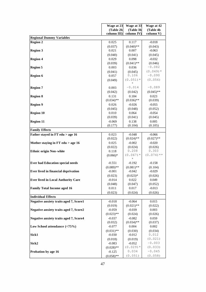
47

Wage at 23 (Table 2b

column III)

Wage at 33 (Table 3b

column IV)

Wage at 42 (Table 4b column V)

Regional Dummy Variables Region 2 0.025 0.117 -0.018

(0.037) (0.040)** (0.043) Region 3 0.021 0.007 -0.063

(0.040) (0.041) (0.045) Region 4 0.029 0.098 -0.032

(0.039) (0.041)** (0.046) Region 5 0.003 0.036 -0.082

(0.041) (0.045) (0.049)* Region 6 0.057 0.106 -0.090

(0.049) (0.051)**

(0.056)

Region 7 0.003 -0.014 -0.089 (0.042) (0.042) (0.045)**

Region 8 0.131 0.184 0.023 (0.034)** (0.036)** (0.039)

Region 9 0.026 -0.026 -0.055 (0.045) (0.048) (0.052)

Region 10 0.010 0.064 -0.054 (0.039) (0.041) (0.045)

Region 11 -0.069 0.138 0.005 (0.177) (0.104) (0.105)

Family Effects Father stayed in FT edu > age 16 0.023 -0.048 -0.066

(0.022) (0.024)** (0.027)** Mother staying in FT edu > age 16 0.025 -0.002 -0.020

(0.022) (0.024) (0.026) Ethnic origin Non-white 0.118 0.208 0.303

(0.066)* (0.067)**

(0.074)**

Ever had Education special needs -0.551 -0.192 -0.158 (0.089)** (0.081)** (0.104)

Ever lived in financial deprivation -0.001 -0.042 -0.029 (0.023) (0.023)* (0.026)

Ever lived in Local Authority Care -0.014 0.022 0.049 (0.048) (0.047) (0.052)

Family Total Income aged 16 0.011 0.017 -0.013 (0.023) (0.024) (0.026)

Individual Effects Negative anxiety traits aged 7, Score1 -0.018 -0.064 0.015

(0.019) (0.021)** (0.022) Negative anxiety traits aged 7, Score2 -0.059 -0.039 0.003

(0.023)** (0.024) (0.026) Negative anxiety traits aged 7, Score4 -0.037 -0.082 0.059

(0.032) (0.034)** (0.037) Low School attendance (<75%) -0.077 0.004 0.002

(0.031)** (0.030) (0.034) Sick1 -0.030 -0.012 0.012

(0.018) (0.019) (0.021) Sick2 -0.083 -0.052 -0.003

(0.028)** (0.029)* (0.033) Probation by age 16 -0.125 0.034 -0.045

(0.058)** (0.051) (0.058)

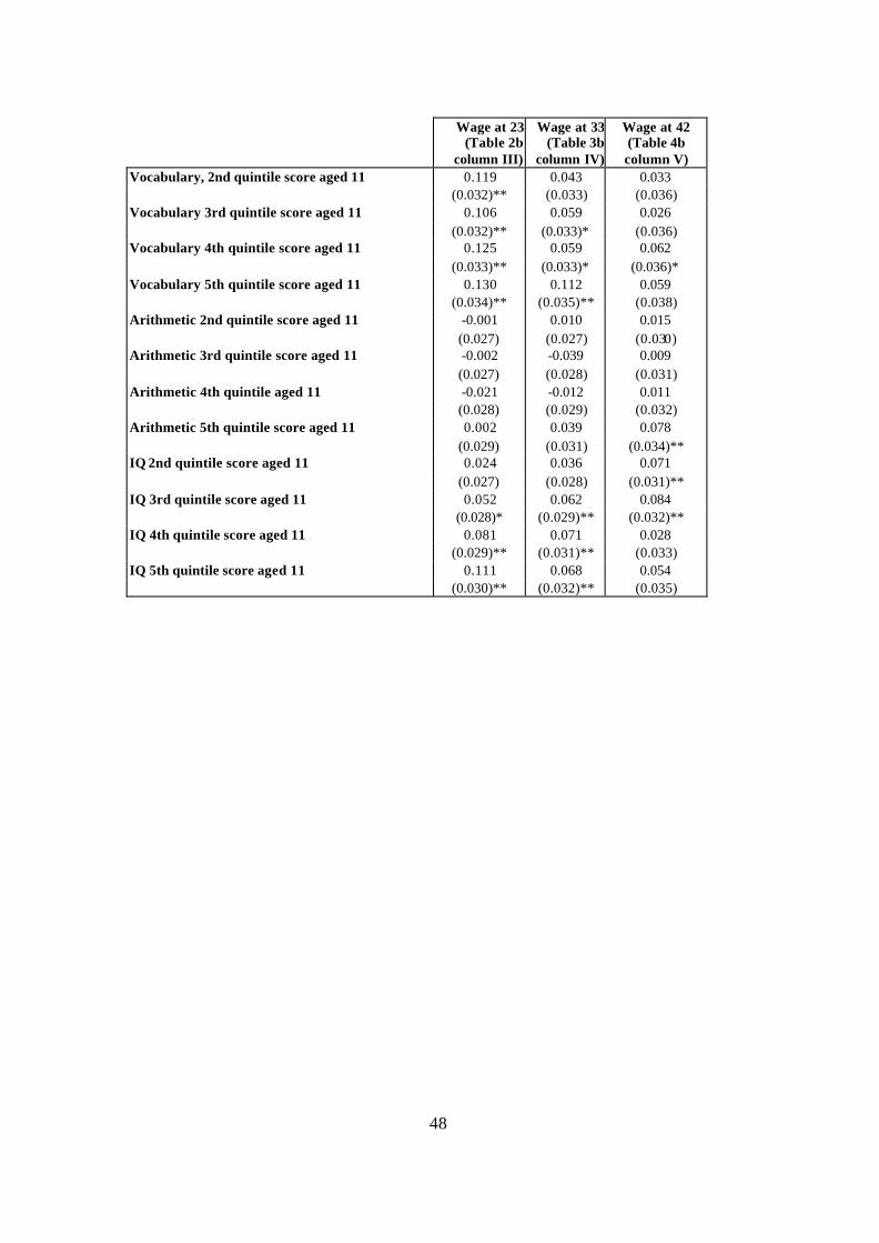
48

Wage at 23

(Table 2b column III)

Wage at 33 (Table 3b

column IV)

Wage at 42 (Table 4b column V)

Vocabulary, 2nd quintile score aged 11 0.119 0.043 0.033 (0.032)** (0.033) (0.036)

Vocabulary 3rd quintile score aged 11 0.106 0.059 0.026 (0.032)** (0.033)* (0.036)

Vocabulary 4th quintile score aged 11 0.125 0.059 0.062 (0.033)** (0.033)* (0.036)*

Vocabulary 5th quintile score aged 11 0.130 0.112 0.059 (0.034)** (0.035)** (0.038)

Arithmetic 2nd quintile score aged 11 -0.001 0.010 0.015 (0.027) (0.027) (0.030)

Arithmetic 3rd quintile score aged 11 -0.002 -0.039 0.009 (0.027) (0.028) (0.031)

Arithmetic 4th quintile aged 11 -0.021 -0.012 0.011 (0.028) (0.029) (0.032)

Arithmetic 5th quintile score aged 11 0.002 0.039 0.078 (0.029) (0.031) (0.034)**

IQ 2nd quintile score aged 11 0.024 0.036 0.071 (0.027) (0.028) (0.031)**

IQ 3rd quintile score aged 11 0.052 0.062 0.084 (0.028)* (0.029)** (0.032)**

IQ 4th quintile score aged 11 0.081 0.071 0.028 (0.029)** (0.031)** (0.033)

IQ 5th quintile score aged 11 0.111 0.068 0.054 (0.030)** (0.032)** (0.035)