Embed Size (px)
Citation preview
1
The Vulcan Project: High resolution fossil fuel combustion CO2 emission fluxes for the United States
Kevin R. Gurney, Daniel L. Mendoza, Yuyu Zhou, Chris Miller, Sarath Geethakumar
Department of Earth and Atmospheric Sciences/Department of Agronomy, Purdue University, 550 Stadium Mall Drive, West Lafayette, IN 47907
Marc L. Fischer, Stephanie de la Rue du Can Atmospheric Science Department, Environmental Energy Technologies Division,
Lawrence Berkeley National Laboratory, 90K-125, Berkeley, CA 94720
ABSTRACT Quantification of fossil fuel CO2 emissions at fine space and time resolution is emerging as a critical need in carbon cycle and climate change research. As atmospheric CO2 measurements expand with the advent of a dedicated remote sensing platform and denser in situ measurements, the ability to close the carbon budget at spatial scales of ~100 km2 and daily timescales requires fossil fuel CO2 inventories at commensurate resolution. Additionally, the growing interest in U.S. climate change policy measures are best served by emissions that are tied to the driving processes in space and time. Here we introduce the Vulcan inventory, a new data product that has quantified fossil fuel CO2 emissions for the U.S. at spatial scales less than 100 km2 and temporal scales as small as hours. This data product, completed for the year 2002, includes detail on combustion technology and forty-eight fuel types through all sectors of the U.S. economy. The Vulcan inventory is built from the decades of local/regional air pollution monitoring and complements these data with census, traffic, and digital road datasets. The Vulcan inventory shows excellent agreement with national-level Department of Energy inventories, in spite of the different approach taken by the DOE to quantify U.S. fossil fuel CO2 emissions. Comparison to the 1°x1° fossil fuel CO2 inventory used widely by the carbon cycle and climate change community prior to the construction of the Vulcan inventory, highlights the space/time biases inherent in the population-based approach. New research has begun on a pilot study in which emissions are allocated in space down to the individual building level and utilizing hourly data-driven traffic flow. The Vulcan effort can be seen as a key component of a national assessment and verification system for greenhouse gas emissions and emissions mitigation. Process-level infrastructure will not only deliver decision support on GHG mitigation and verification, but can deliver multiple benefits such as energy planning, local decision support, public outreach, and industrial cost savings.
2
INTRODUCTION Improving the quantitative understanding of the global carbon cycle has emerged as a central element in advancing our understanding of climate change and climate change projections, not to mention deepening our understanding of ecosystem level biogeochemical principles (1). Recent research has highlighted the importance of feedbacks between climate change and carbon uptake in the oceans and land, emphasizing the considerable spread in projected CO2 due to uncertainties in surface-atmosphere exchange (2). The single largest net flux of carbon between the surface and the atmosphere is that due to the combustion of fossil fuels and cement production, recently estimated at 8.4 GtC/year for the year 2006 (3). More importantly, quantitative assessment of biotic exchange on land and exchange with the oceans relies critically on the accuracy of both the incremental change of CO2 in the Earth’s atmosphere and the fossil fuel carbon flux from the surface. This is due to the fact that the surface-atmosphere exchange, particularly that between the terrestrial biosphere and the atmosphere, is commonly solved as the residual in large-scale budget assessments (4). Fossil fuel CO2 inventories began as an accounting exercise based on the production/consumption of fossil fuels at the national scale (5). In most cases, little sub-national allocation of the emissions was performed because the initial purpose – understanding 20th century global climate change – required little sub-national information. Thus, the most common spatiotemporal distribution of fossil fuel CO2 emissions occurred at an annual timescale and at the national spatial scale. Starting in the 1980s, research was begun to further subdivide these emissions into finer spatial and temporal scales (6). By the beginning of the 21st century, fossil fuel CO2 emissions had been produced which were resolved globally, at the 1° x 1° spatial scale and most commonly at an annual time scale (7,8). This sub-national downscaling in space, however, was achieved through a spatial proxy such as population density statistics. The most recent work, prior to the results reported here, has quantified emissions at the scale of U.S. states/monthly (9-13) with two studies estimating and analyzing CO2 fluxes from the power production sector down to the facility level (14, 15). In the last decade, there has been a growing need, from both the science and policymaking communities, for quantification of the complete fossil fuel CO2 emissions at space and time scales finer than what has been produced thus far (16, 17), Carbon cycle science requires more accurate and more finely resolved quantification due to downscaling of carbon budget and inverse approaches, which use space/time patterns of atmospheric CO2 to infer exchange of carbon with the oceans and the terrestrial biosphere (18). These scientific needs have contributed to the planned launch of the Orbiting Carbon Observatory (OCO), which will measure the column concentration of atmospheric CO2 with individual sample footprints of 2.9 km2 and a 10.3 km wide field of view (19). The policymaking community in the U.S. has also recognized the need for accurate, highly resolved CO2 emissions due to the emerging requirements of proposed carbon trading systems or sectoral emissions caps (20).
To answer this growing need for better resolution, accuracy and linkage to the underlying emission drivers, research was begun on the Vulcan project. This paper serves as the first
3
complete description of the methods and results emerging from this effort in which U.S., process-driven, fuel-specific, fossil fuel CO2 emissions were quantified at scales finer than 100 km2/hourly for the year 2002. We present the data sources and methods used to quantify fossil fuel CO2 and the techniques used to perform spatial and temporal allocation. We quantify the results across a number of different dataset dimensions and compare these results to inventories built at coarser scales. Lastly, we describe the implications for carbon cycle science by quantifying the differences between the Vulcan inventory and the widely-used predecessor inventory in terms of atmospheric CO2 concentrations. BODY Methods Data sources
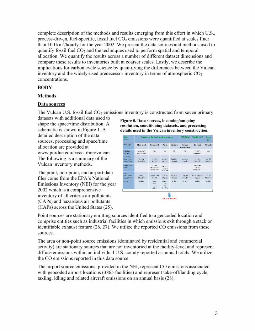
The Vulcan U.S. fossil fuel CO2 emissions inventory is constructed from seven primary datasets with additional data used to shape the space/time distribution. A schematic is shown in Figure 1. A detailed description of the data sources, processing and space/time allocation are provided at www.purdue.edu/eas/carbon/vulcan. The following is a summary of the Vulcan inventory methods.
The point, non-point, and airport data files come from the EPA’s National Emissions Inventory (NEI) for the year 2002 which is a comprehensive inventory of all criteria air pollutants (CAPs) and hazardous air pollutants (HAPs) across the United States (25). Point sources are stationary emitting sources identified to a geocoded location and comprise entities such as industrial facilities in which emissions exit through a stack or identifiable exhaust feature (26, 27). We utilize the reported CO emissions from these sources. The area or non-point source emissions (dominated by residential and commercial activity) are stationary sources that are not inventoried at the facility-level and represent diffuse emissions within an individual U.S. county reported as annual totals. We utilize the CO emissions reported in this data source. The airport source emissions, provided in the NEI, represent CO emissions associated with geocoded airport locations (3865 facilities) and represent take-off/landing cycle, taxiing, idling and related aircraft emissions on an annual basis (28).
Figure 0. Data sources, incoming/outgoing resolution, conditioning datasets, and processing details used in the Vulcan inventory construction.
4
Emissions due to aircraft, beyond the takeoff/landing cycle and emissions captured in the NEI airport database, are taken directly from the Aero2K aircraft CO2 emissions inventory, defined on a three-dimensional 1°x1° degree grid (29).
Because of the reliability of direct CO2 monitoring, continuous stack monitoring data provided through the DOE/EIA and the EPA Clean Air Market Division (CAMD) Emission Tracking System/Continuous Emissions Monitoring (ETS/CEM) for electrical generating units (EGUs)†, are utilized (15).
The onroad mobile emissions are based on a combination of county-level data and standard internal combustion engine stochiometry. The county-level data comes from the National Mobile Inventory Model (NMIM) County Database (NCD) for 2002 which quantifies the vehicle miles traveled in a county by month, specific to vehicle class and road type (30). The Mobile6.2 combustion emissions model is used to generate CO2 emission factors on a per mile basis given inputs such as fleet information, temperature, fuel type, and vehicle speed (31, 32). Nonroad emissions are structured similarly to the onroad mobile emissions data and consist of mobile sources that do not travel on designated roadways. These data, retrieved from the NMIM NCD, have a space/time resolution of county/month and are reported as activity (number of hour/month vehicle runs), population and a CO2 emission factor specific to vehicle class (28, 33).
Emissions calculation For datasets that do not directly provide CO2 emissions, CO and CO2 emission factors are used. These factors are specific to the combustion process and the 48 fuels tracked in the Vulcan system. CO emission factors are often supplied in the incoming datasets but are often missing or inconsistent with independent data. In many cases, therefore, standard emission factor databases are used to assign values to each combustion technology/fuel combination‡ (34, 25). Where standard factors are not available, default emission factors are used. Emission factors for CO2 are based on the fuel carbon content and assume a gross calorific value or high heating value, as this is the convention most commonly used in the U.S. and Canada (36).
The basic process by which CO2 emissions are created is as follows: (1)
where C, is the emitted amount of carbon, PE is the equivalent amount of uncontrolled criteria pollutant emissions (CO emissions), p is the combustion process (e.g. industrial 10 MMBTU boiler, industrial gasoline reciprocating turbine), f is the fuel type (e.g. natural gas or bituminous coal), PF is the emission factor associated with the criteria
† United States Environmental Protection Agency, Clean Air Markets – Data and Maps, http://camddataandmaps.epa.gov/gdm/index.cfm, accessed June 10, 2008.
‡ Technology Transfer Network Clearinghouse for Inventories & Emissions Factor, WebFIRE, December 2005, http://cfpub.epa.gov/oarweb/index.cfm?action=fire.main, accessed 06/10/08.
5
pollutant, and CF is the emission factor associated with CO2. Percent oxidation level is embedded in the CO2 emission factor.
Spatial/temporal downscaling For those data sources that are not geocoded (mobile and non-point sources), allocation of emissions in space is performed through the use of additional datasets. Downscaling of the residential and commercial emissions in addition to the small amount of industrial sector emissions reported in the non-point NEI files are performed through use of census tract-level spatial surrogates prepared by the EPA (37).
Onroad emissions are also spatially downscaled from the county level by allocating the hourly/county/road/vehicle-specific CO2 emissions onto roadways using a GIS road atlas§. The monthly/county/road/vehicle-specific CO2 emissions are further subdivided in time using Weight In Motion (WIM) data obtained from the San Jose Valley traffic department (38). Temporal downscaling to monthly time increments increments by state for the residential and commercial sector was performed for the non-point data sources by state and sector. Data on state-level, sector-based natural gas delivered to consumers from the DOE/EIA (39) was used to construct monthly fractions for the year 2002. In order to facilitate atmospheric transport modeling, all of these emission sources are placed onto a common 10 km x 10 km grid. Geocoded sources are evenly spread across the resident grid cell while onroad sources are broken at the edges of the grid cells and summed into the cells to which they belong. Non-point sources are downscaled from the Census tract to 10 km via area-based weighting.
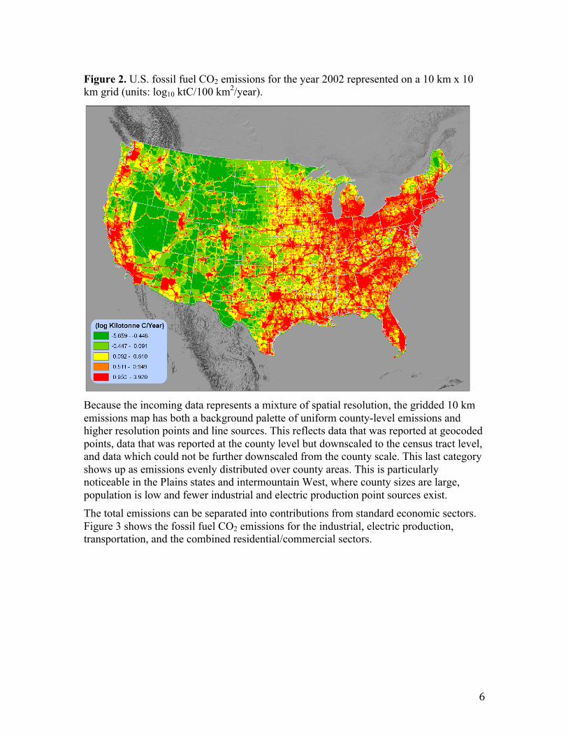
Results and discussion Figure 2 shows the total 2002 U.S. fossil fuel CO2 emissions, represented on a 10 km x 10 km grid. Emissions are most readily associated with population centers but interstate highways and concentrations of industrial activity are also evident.
§ A collection of spatial data for use in GIS‐based applications. Washington, D.C.: The Bureau. worldcat.org/oclc/52933703&referer=one_hit
6
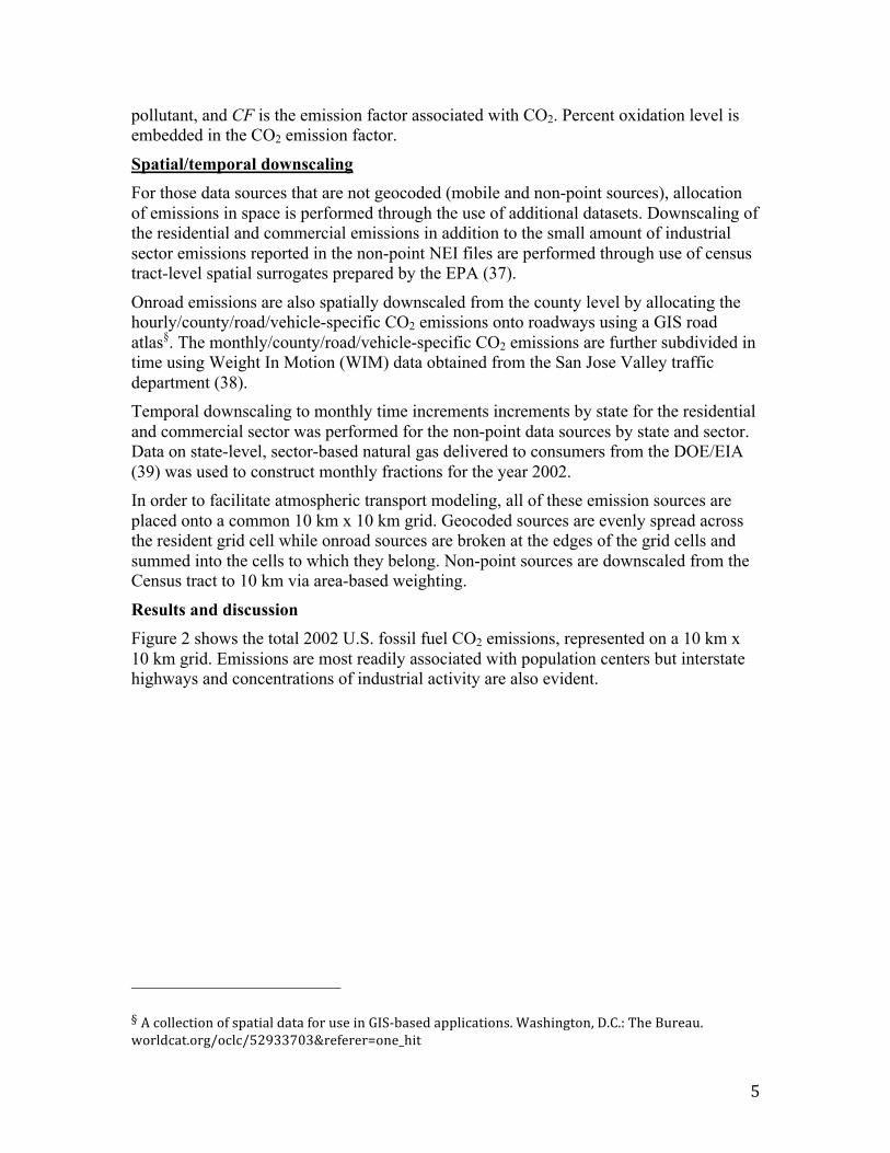
Figure 2. U.S. fossil fuel CO2 emissions for the year 2002 represented on a 10 km x 10 km grid (units: log10 ktC/100 km2/year).
Because the incoming data represents a mixture of spatial resolution, the gridded 10 km emissions map has both a background palette of uniform county-level emissions and higher resolution points and line sources. This reflects data that was reported at geocoded points, data that was reported at the county level but downscaled to the census tract level, and data which could not be further downscaled from the county scale. This last category shows up as emissions evenly distributed over county areas. This is particularly noticeable in the Plains states and intermountain West, where county sizes are large, population is low and fewer industrial and electric production point sources exist. The total emissions can be separated into contributions from standard economic sectors. Figure 3 shows the fossil fuel CO2 emissions for the industrial, electric production, transportation, and the combined residential/commercial sectors.
7
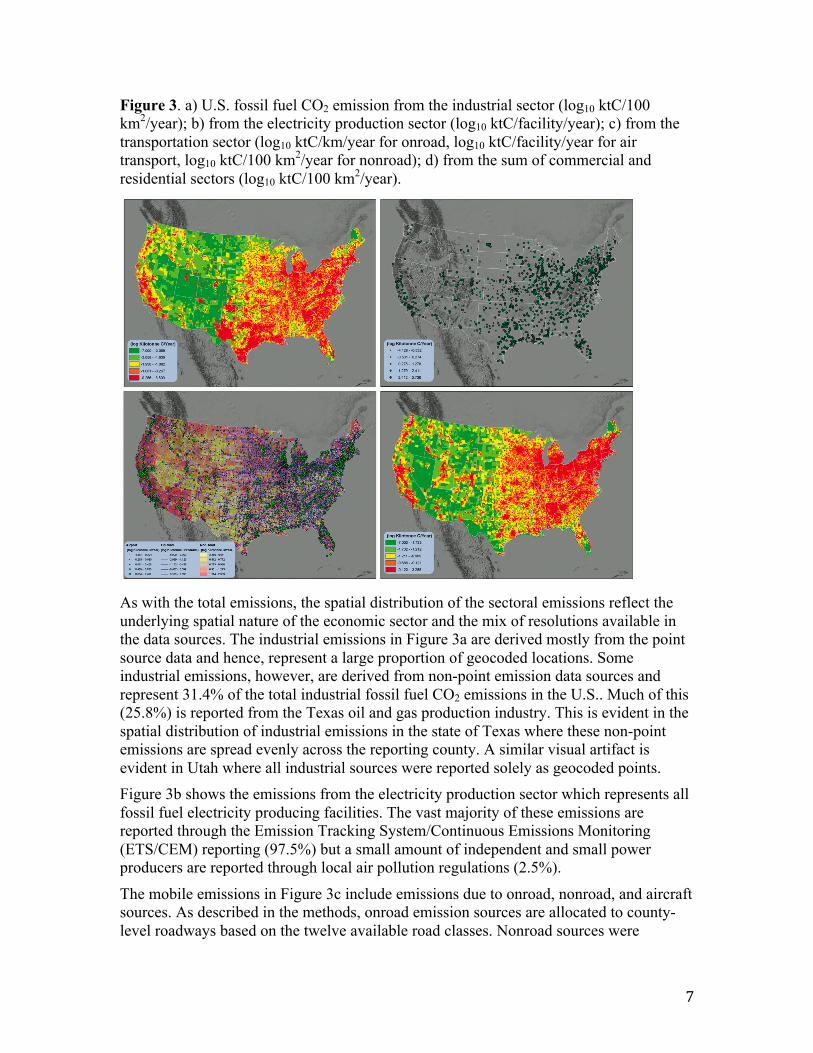
Figure 3. a) U.S. fossil fuel CO2 emission from the industrial sector (log10 ktC/100 km2/year); b) from the electricity production sector (log10 ktC/facility/year); c) from the transportation sector (log10 ktC/km/year for onroad, log10 ktC/facility/year for air transport, log10 ktC/100 km2/year for nonroad); d) from the sum of commercial and residential sectors (log10 ktC/100 km2/year).
As with the total emissions, the spatial distribution of the sectoral emissions reflect the underlying spatial nature of the economic sector and the mix of resolutions available in the data sources. The industrial emissions in Figure 3a are derived mostly from the point source data and hence, represent a large proportion of geocoded locations. Some industrial emissions, however, are derived from non-point emission data sources and represent 31.4% of the total industrial fossil fuel CO2 emissions in the U.S.. Much of this (25.8%) is reported from the Texas oil and gas production industry. This is evident in the spatial distribution of industrial emissions in the state of Texas where these non-point emissions are spread evenly across the reporting county. A similar visual artifact is evident in Utah where all industrial sources were reported solely as geocoded points. Figure 3b shows the emissions from the electricity production sector which represents all fossil fuel electricity producing facilities. The vast majority of these emissions are reported through the Emission Tracking System/Continuous Emissions Monitoring (ETS/CEM) reporting (97.5%) but a small amount of independent and small power producers are reported through local air pollution regulations (2.5%).
The mobile emissions in Figure 3c include emissions due to onroad, nonroad, and aircraft sources. As described in the methods, onroad emission sources are allocated to county-level roadways based on the twelve available road classes. Nonroad sources were
8
distributed evenly throughout the reporting county and aircraft sources (landing/takeoff and airborne) are allocated to geocoded airport locations. Onroad emissions are the dominant source within the mobile sector, representing 79.4% of the total, followed by aircraft emissions (11.8%) and nonroad emissions (8.8%). Both the density of urban onroad emissions and the presence of interstate travel are evident in Figure 3c as is the importance of airport emissions.
Figure 3d represents the sum of residential and commercial emissions. Both emission sectors follow population density with the residential sector somewhat less concentrated in population centers than commercial emissions. This is likely due to the fact that commercial buildings and businesses are more tightly related to urban development and employee density whereas residential structures are more dispersed into the suburban and exurban landscape.
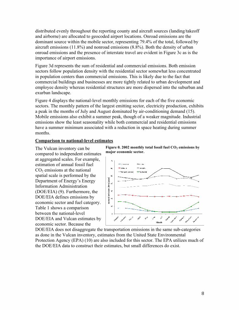
Figure 4 displays the national-level monthly emissions for each of the five economic sectors. The monthly pattern of the largest emitting sector, electricity production, exhibits a peak in the months of July and August dominated by air-conditioning demand (15). Mobile emissions also exhibit a summer peak, though of a weaker magnitude. Industrial emissions show the least seasonality while both commercial and residential emissions have a summer minimum associated with a reduction in space heating during summer months. Comparison to national-level estimates
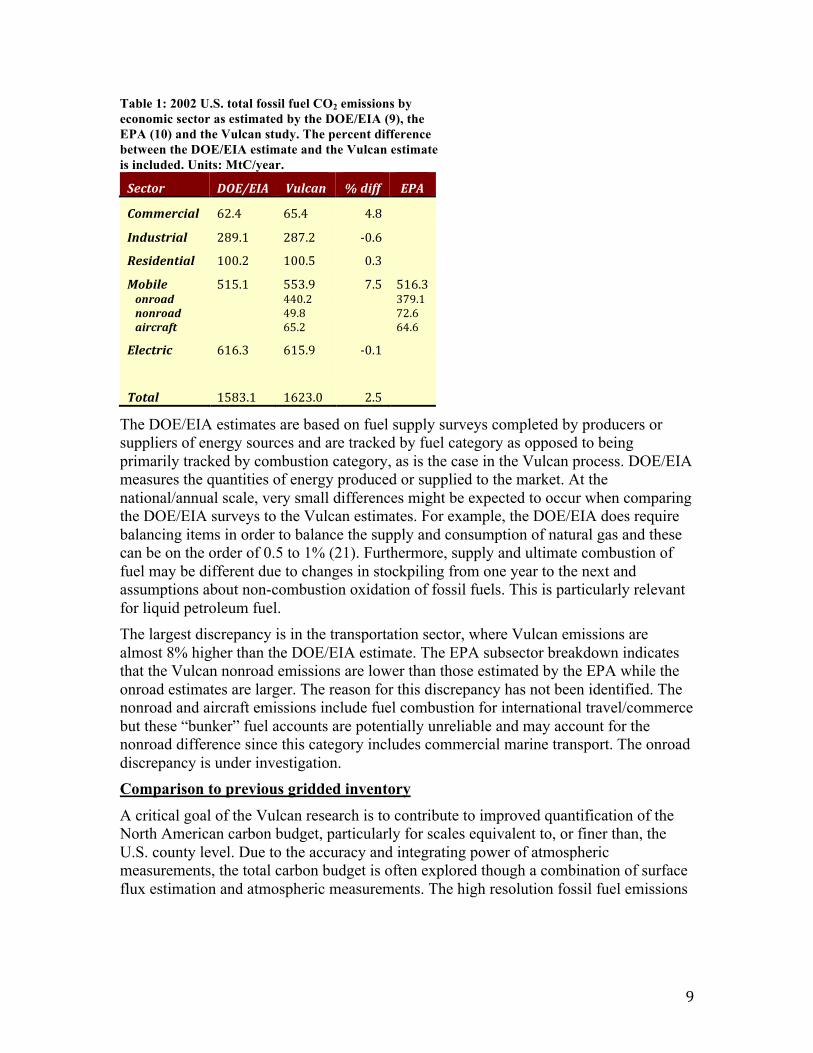
The Vulcan inventory can be compared to independent estimates at aggregated scales. For example, estimation of annual fossil fuel CO2 emissions at the national spatial scale is performed by the Department of Energy’s Energy Information Administration (DOE/EIA) (9). Furthermore, the DOE/EIA defines emissions by economic sector and fuel category. Table 1 shows a comparison between the national-level DOE/EIA and Vulcan estimates by economic sector. Because the DOE/EIA does not disaggregate the transportation emissions in the same sub-categories as done in the Vulcan inventory, estimates from the United State Environmental Protection Agency (EPA) (10) are also included for this sector. The EPA utilizes much of the DOE/EIA data to construct their estimates, but small differences do exist.
Figure 0. 2002 monthly total fossil fuel CO2 emissions by major economic sector.
9
Table 1: 2002 U.S. total fossil fuel CO2 emissions by economic sector as estimated by the DOE/EIA (9), the EPA (10) and the Vulcan study. The percent difference between the DOE/EIA estimate and the Vulcan estimate is included. Units: MtC/year.
Sector DOE/EIA Vulcan % diff EPA
Commercial 62.4 65.4 4.8
Industrial 289.1 287.2 ‐0.6
Residential 100.2 100.5 0.3
Mobile 515.1 553.9 7.5 516.3 onroad 440.2 379.1 nonroad 49.8 72.6 aircraft 65.2 64.6
Electric 616.3 615.9 ‐0.1
Total 1583.1 1623.0 2.5
The DOE/EIA estimates are based on fuel supply surveys completed by producers or suppliers of energy sources and are tracked by fuel category as opposed to being primarily tracked by combustion category, as is the case in the Vulcan process. DOE/EIA measures the quantities of energy produced or supplied to the market. At the national/annual scale, very small differences might be expected to occur when comparing the DOE/EIA surveys to the Vulcan estimates. For example, the DOE/EIA does require balancing items in order to balance the supply and consumption of natural gas and these can be on the order of 0.5 to 1% (21). Furthermore, supply and ultimate combustion of fuel may be different due to changes in stockpiling from one year to the next and assumptions about non-combustion oxidation of fossil fuels. This is particularly relevant for liquid petroleum fuel. The largest discrepancy is in the transportation sector, where Vulcan emissions are almost 8% higher than the DOE/EIA estimate. The EPA subsector breakdown indicates that the Vulcan nonroad emissions are lower than those estimated by the EPA while the onroad estimates are larger. The reason for this discrepancy has not been identified. The nonroad and aircraft emissions include fuel combustion for international travel/commerce but these “bunker” fuel accounts are potentially unreliable and may account for the nonroad difference since this category includes commercial marine transport. The onroad discrepancy is under investigation. Comparison to previous gridded inventory
A critical goal of the Vulcan research is to contribute to improved quantification of the North American carbon budget, particularly for scales equivalent to, or finer than, the U.S. county level. Due to the accuracy and integrating power of atmospheric measurements, the total carbon budget is often explored though a combination of surface flux estimation and atmospheric measurements. The high resolution fossil fuel emissions
10
data product, generated by Antoinette Brenkert†, widely used in carbon cycle studies, was a 1°x1° emissions product based on 1995 national-level fossil fuel consumption combined with population density (7, 8).
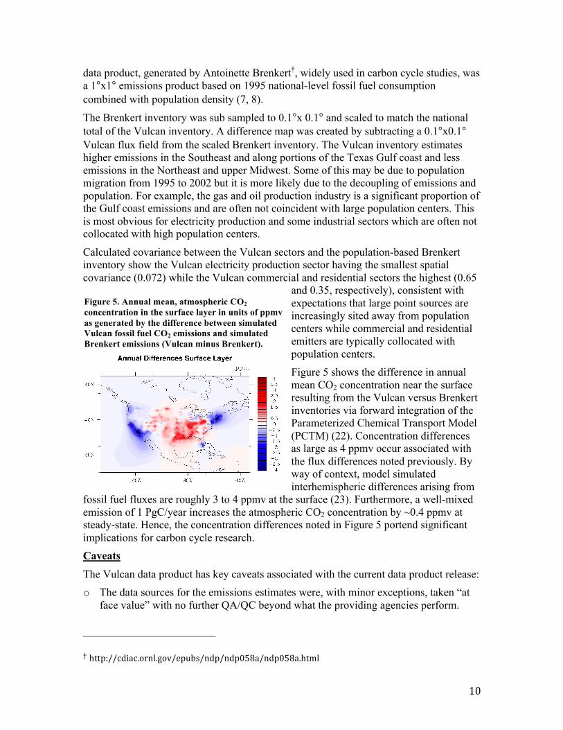
The Brenkert inventory was sub sampled to 0.1°x 0.1° and scaled to match the national total of the Vulcan inventory. A difference map was created by subtracting a 0.1°x0.1° Vulcan flux field from the scaled Brenkert inventory. The Vulcan inventory estimates higher emissions in the Southeast and along portions of the Texas Gulf coast and less emissions in the Northeast and upper Midwest. Some of this may be due to population migration from 1995 to 2002 but it is more likely due to the decoupling of emissions and population. For example, the gas and oil production industry is a significant proportion of the Gulf coast emissions and are often not coincident with large population centers. This is most obvious for electricity production and some industrial sectors which are often not collocated with high population centers.
Calculated covariance between the Vulcan sectors and the population-based Brenkert inventory show the Vulcan electricity production sector having the smallest spatial covariance (0.072) while the Vulcan commercial and residential sectors the highest (0.65
and 0.35, respectively), consistent with expectations that large point sources are increasingly sited away from population centers while commercial and residential emitters are typically collocated with population centers. Figure 5 shows the difference in annual mean CO2 concentration near the surface resulting from the Vulcan versus Brenkert inventories via forward integration of the Parameterized Chemical Transport Model (PCTM) (22). Concentration differences as large as 4 ppmv occur associated with the flux differences noted previously. By way of context, model simulated interhemispheric differences arising from
fossil fuel fluxes are roughly 3 to 4 ppmv at the surface (23). Furthermore, a well-mixed emission of 1 PgC/year increases the atmospheric CO2 concentration by ~0.4 ppmv at steady-state. Hence, the concentration differences noted in Figure 5 portend significant implications for carbon cycle research. Caveats
The Vulcan data product has key caveats associated with the current data product release: o The data sources for the emissions estimates were, with minor exceptions, taken “at
face value” with no further QA/QC beyond what the providing agencies perform.
† http://cdiac.ornl.gov/epubs/ndp/ndp058a/ndp058a.html
Figure 5. Annual mean, atmospheric CO2 concentration in the surface layer in units of ppmv as generated by the difference between simulated Vulcan fossil fuel CO2 emissions and simulated Brenkert emissions (Vulcan minus Brenkert).
11
o In terms of introduced uncertainty, assignment of non-CO2 pollutant emission factors contain the greatest amount of uncertainty and unaccounted for variability. Though formal uncertainty associated with the non-CO2 pollutant emission factors has not been presented here, extensive uncertainty and sensitivity analysis is underway and will accompany future releases of the Vulcan data product.
o The downscaling of the non-point sources relies on the use of building square footage. Other predictive factors not considered in the sub-county downscaling would be variables such as building age, occupancy, and non-space heating share of fuel use, .
o The sub-monthly temporal downscaling of the mobile emissions remains limited in terms of capturing true spatial variability.
o The 48 fuels tracked in the Vulcan inventory are represented by U.S.-average heat contents, carbon contents and carbon fraction oxidized. This overlooks potential spatial and temporal variation in these parameters.
Implications The Vulcan inventory has wide-ranging implications for carbon cycle and climate change research and utility for national legislation on climate change and energy policy. As the largest net land-atmosphere flux, fossil fuel CO2 plays a key role in atmospheric CO2 inversions, widely used to identify and understand the net terrestrial flux. Space/time biases in the fossil fuel flux are directly aliased into the net terrestrial flux in these studies (4). As inversion studies move to smaller space/time scales, the fossil fuel CO2 flux must be accurately quantified at smaller space/time scales. This is particularly true as remotely sensed CO2 observations become available (19). The Vulcan inventory also paves the way for incorporation of much finer, process-driven emissions into integrated assessment studies which currently utilize spatially coarse emission projections driven from indirect measures such as population and economic growth. Finally, the Vulcan inventory can provide a carbon trading system with a single, science-driven inventory platform. This could widen the scale and sectoral detail for carbon trading. It could also offer a method by which progress in emissions mitigation can be tracked and performance confirmed. This last point is crucial in that currently there is no systematic way to evaluate the progress of mitigation measures, an essential component of assessing and judging success as the U.S. constructs legislative measures on climate change mitigation.
An opportunity exists to build an assessment and verification system for greenhouse gases that incorporates inventory and accounting rules and data collection with measurement of greenhouse gases in the atmosphere. In order for atmospheric measurements to provide evaluation of inventories, emissions must be placed accurately in space and time and do so at scales that approximate atmospheric measurement footprints. With the advent of remote sensing strategies to measure greenhouse gases and the continued growth in high frequency in situ and aircraft measurements, these footprints are approach areas on the order of 10s of km2.
12
Furthermore, a process-based or relationship driven model-data system that tracks greenhouse gas precursor materials and processes through the economic system to the point of emission offers a variety of value-added benefits over a simple inventory. For example, tracking fossil fuel from the point at which it enters the U.S. economy in raw form through processing, transport and combustion offers the opportunity for scenario development. “What-if” questions such as fuel switching, technology change, and conservation can be posed and simulated in order to arrive at physically consistent conclusions. This offers a powerful platform for local decision support in greenhouse gas mitigation. The addition of multiple data streams in order to support such a process-driven system actually improves emissions uncertainty by leveraging far more information from related datasets. A process-based model-data system would not only provide assessment and verification of greenhouse gas emissions, but offers a platform for a variety of other scientific disciplines such as energy analysis, sociology, urban policy and development, transportation studies, etc. Online visualization and the potential for interaction offers the opportunity for local knowledge to be incorporated into a model-data system which both builds space/time accuracy and is a powerful engagement and outreach tool. Near-term research direction Future research direction for the Vulcan Project includes quantifying Canada and Mexico in order to complete the entire North American inventory. Work has also begun on comparison to recently-completed state/month level inventories built from fuel sales and supply (13, 9). The 10 km x 10 km Vulcan inventory for each of the sectoral contributions has recently been placed within the Google Earth platform and further work is planned to provide more of the detail within the complete Vulcan data product such as a “native” resolution product (geocoded points, roads, etc) and combustion category and fuel types.
Moving the Vulcan emissions estimate beyond the year 2002 will also be accomplished in the near-term. First, the incorporation of NEI datasets from 1999 and 2005 will be accomplished. Then, years in between these data releases will be estimated through the use of DOE EIA fuel data.
Work has recently been proposed to accomplish a global fossil fuel CO2 inventory and this will include both in situ and remote-sensing datasets and an assimilation system. This will not attain the space/time resolution of the Vulcan inventory but will significantly improve the curent estimates that are constrained at the national/annual level only.
Finally, research has begun on building a fossil fuel CO2 inventory at the scale of individual buildings in near real-time through a combination of in-situ measurements, remote sensing, and energy systems modeling. This project, called “Hestia” is currently utilizing the city of Indianapolis as a first pilot location and is complemented by airborne CO2 flux measurement campaigns from low-flying light aircraft (24). CONCLUSIONS The Vulcan inventory quantifies all fossil fuel CO2 emissions from the United States at spatial scales below the county level and temporal scales below the monthly level. Constructed in order to support carbon cycle science research in North America, it relies
13
on a series of datasets from the EPA, DOE, US Census, and DOT. These initial datasets are further conditioned to place the emissions in space and time and manipulated to produce. The Vulcan inventory, completed for the year 2002, includes detail on combustion technology and all fuel types through all sectors of the U.S. economy. The Vulcan inventory shows excellent agreement with national-level Department of Energy inventories, in spite of the different approach taken by the DOE to quantify U.S. fossil fuel CO2 emissions. Comparison to the 1°x1° fossil fuel CO2 inventory used widely by the carbon cycle and climate change community prior to the construction of the Vulcan inventory, highlights the space/time biases inherent in the population-based approach. New research has begun on a pilot study in which emissions are allocated in space down to the individual building level and utilizing hourly data-driven traffic flow. Near-term goals for the Vulcan project are to include Canada and Mexico, and attempt a coarser-resolution inventory at the global scale. The Vulcan effort can be seen as a key component of a national assessment and verification system for greenhouse gas emissions and emissions mitigation. Process-level infrastructure will not only deliver decision support on GHG mitigation and verification, but can deliver multiple benefits such as energy planning, local decision support, public outreach, and industrial cost savings.

14
Acknowledgements
Support for the Vulcan research provided by grant NASA, grant Carbon/04-0325-0167 and DOE grant DE-AC02-05CH11231. Computational support provided by the Rosen Center for Advanced Computing (Broc Seib and William Ansley) and the Envision Center (Bedrich Benes and Nathan Andrysco). Thanks to Simon Ilyushchenko of Google Inc., Dennis Ojima and Steve Knox of Colorado State university and the CO2FFEE group for helpful discussion and input.
15
References 1. Denman, K.L. et al. (2007), Couplings Between Changes in the Climate System and
Biogeochemistry in Climate Change 2007, The Physical Science Basis, contribution of Working Group I to the Fourth Assessment Report of the IPCC.
2. Friedlingstein, P., et al. (2006), Climate-Carbon Cycle Feedback Analysis: Results from the C4MIP Model Intercomparison, J. Climate, 19: 3337-3353.
3. Canadell, J.G., et al. (2007), Contributions to accelerating atmospheric CO2 growth from economic activity, carbon intensity, and efficiency of natural sinks, PNAS, 104 (47): 18866-18870.
4. Gurney, K.R., Y.H. Chen, T. Maki, S.R. Kawa, A. Andrews, Z. Zhu (2005), Sensitivity of Atmospheric CO2 Inversion to Seasonal and Interannual Variations in Fossil Fuel Emissions, J. Geophys. Res. 110 (D10): 10308-10321.
5. Marland, G., R.M. Rotty, and N.L. Treat (1985), CO2 from fossil fuel burning: global distribution of emissions, Tellus, 37B: 243-258.
6. Rotty, R. (1983), Distribution of and changes in industrial carbon dioxide production, J. Geophys. Res., 88 (C2): 1301-1308.
7. Andres, R.J. Marland, G., Fung, I. and E. Matthews (1996), A 1 x 1 distribution of carbon dioxide emissions from fossil fuel consumption and cement manufacture, 1950-1990, Glob. Biogeochem. Cyc., 10: 419-429.
8. Olivier, J.G.J. et al. (1999), Sectoral emission inventories of greenhouse gases for 1990 on a per country basis as well as on 1 x 1. Environmental Science & Policy, 2: 241-264.
9. Department of Energy/Energy Information Administration (2007), Emission of Greenhouse Gases in the United States 2006, Energy Information Administration, Office of Integrated Analysis and Forecasting, U.S. Department of Energy, Washington, DC 20585, DOE/EIA-0573.
10. United States Environmental Protection Agency (2008), Inventory of U.S. Greenhouse Gas Emissions and Sinks: 1990-2006, U.S. Environmental Protection Agency, Washington, DC 20460.
11. Blasing, T.J., C.T. Broniak, and G. Marland (2005), State-by-state carbon dioxide emissions from fossil fuel use in the United States 1960-2000, Mitig. Adap. Strat. Glob. Change, 10: 659-674.
12. Blasing, T.J., C.T. Broniak, and G. Marland (2005), The annual cycle of fossil-fuel carbon dioxide emissions in the United States, Tellus, 57B: 107-115.
13. Gregg, J.S. and R.J. Andres (2008), A method for estimating the temporal and spatial patterns of carbon dioxide emissions from national fossil-fuel consumption, Tellus, 60B: 1-10.
14. Ackerman, K. V., and E. T. Sundquist (2008), Comparison of two U.S. power-plant carbon dioxide emissions data sets, Environ. Sci. Technol., 42: 5688–5693.
15. Petron, G., P. Tans, G. Frost, D. Chao, and M. Trainer (2008), High resolution emissions of CO2 from power generation in the USA, J. Geophys. Res., 113: doi:10.1029/2007/JG000602.
16. Gurney, K.R. et al. (2007), Research needs for process-driven, finely resolved fossil fuel carbon dioxide emissions, EOS Trans., 88 (49): 542-543.
17. Denning, A.S. et al. (2005), Science Implementation Strategy for the North American Carbon Program. Report of the NACP Implementation Strategy Group of the U.S.
16
Carbon Cycle Interagency Working Group. Washington, DC: U.S. Carbon Cycle Science Program, 68 pp.
18. Gurney, K.R., et al. (2002), Towards robust regional estimates of CO2 sources and sinks using atmospheric transport models, Nature, 415: 626-630.
19. Crisp, D. et al. (2004) The Orbiting Carbon Observatory (OCO) Mission. Advances in Space Research, 34(4): 700-709.
20. Lieberman, J. and M. Warner (2007), America’s Climate Security Act of 2007, S.2191, 110th Congress, U.S. Senate.
21. Department of Energy/Energy Information Administration (2007), Natural Gas Annual 2006, Energy Information Administration, Office of Oil and Gas, U.S. Department of Energy, Washington, DC 20585, DOE/EIA-0131.
22. Kawa, S. R., D. J. Erickson III, S. Pawson, and Z. Zhu (2004), Global CO2 transport simulations using meteorological data from the NASA data assimilation system, J. Geophys. Res., 109 (D18312): doi:10.1029/2004JD004554.
23. Denning, A.S., I.Y. Fung, and D. Randall (1995), Latitudinal gradient of atmospheric CO2 due to seasonal exchange with land biota, Nature 376: 240–243.
24. Ross, K., P. Shepson, B. Stirm, A. Karion, C. Sweeney, and K. Gurney (2009), Aircraft-Based Measurements of the Carbon Footprint of Indianapolis, in prep
25. United States Environmental Protection Agency (2005), Emissions Inventory Guidance for Implementation of Ozone and Particulate Matter National Ambient Air Quality Standards (NAAQS and Regional Haze Regulations), Emissions Inventory Group, Emissions, Monitoring and Analysis Division, Office of Air Quality Planning and Standards, U.S. Environmental Protection Agency, Research Triangle Park, NC 27711, EPA-454/R-05-001.
26. United States Environmental Protection Agency (2006), Documentation for the Final 2002 Point Source National Emissions Inventory, Emission Inventory and Analysis Group, Air Quality and Anlysis Division, U.S. Environmental Protection Agency, Research Triangle Park, NC 27711, February 10.
27. Eastern Research Group, Inc (2001), Introduction to Stationary Point Source Emissions Inventory Development, Volume II, Chapter 1, prepared for: Point Sources Committee, Emission Inventory Improvement Program, May.
28. United States Environmental Protection Agency (2005), Documentation for Aircraft, Commercial Marine Vessel, Locomotive, and Other Nonroad Components of the National Emissions Inventory, Volume I – Methodology, Emission Factor and Inventory Group (D205-01), Emissions, Monitoring and Analysis Division, U.S. Environmental Protection Agency, Research Triangle Park, North Carolina 27711, EPA Contract No.: 68-D-02-063, September.
29. Eyers, C.J., et al. (2004), AERO2k Global Aviation Emissions Inventories for 2002 and 2025, Center for Air Transport and the Environment, QINETIQ/04/01113, December.
30. United States Environmental Protection Agency (2005) Office of Transportation and Air Quality, EPA’s National Mobile Inventory Model (NMIM), A consolidated emissions modeling system for MOBILE6 and NONROAD, Assesssment and Standards Division, Office of Transportation and Air Quality, U.S. Environmental Protection Agency, EPA420-R-05-024, December.

17
31. United States Environmental Protection Agency (2001), Fleet Characterization Data for MOBILE6: Development and Use of Age Distributions, Average Annual Mileage Accumulation Rates, and Projected Vehicle Counts for Use in MOBILE6, United States Environmental Protection Agency, EPA420-R-01-047, September.
32. Harrigton, W. (1998), A Behavioral Analysis of EPA’s MOBILE Emission Factor Model, Discussion Paper 98-47, Resources for the Future, September, Washington DC.
33. United States Environmental Protection Agency (2005), User’s Guide for the Final NONROAD2005 Model, Assessment and Standards, Division Office of Transportation and Air Quality U.S. Environmental Protection Agency, December.
34. United States Environmental Protection Agency (1997), Procedures for Preparing Emission Factor Documents, Office of Air Quality Planning and Standards, Office of Air and Radiation, U.S. Environmental Protection Agency, Research Triangle Park, NC 27711, November, EPA-454/R-95-015 Revised.
35. United States Environmental Protection Agency (2006), Draft Detailed Procedures for Preparing Emissions Factors, U.S. Environmental Protection Agency, Office of Air Quality Planning and Standards, Emissions Monitoring and Analysis Division, Emissions Factors and Policy Applications Group, Research Triangle Park, NC 27711, June 29.
36. URS (2003), Greenhouse Gas Emission Factor Review, Final Technical Memorandum, URS Corporation, Austin, Texas, February 3.
37. DynTel (2002) Spatial Allocation Information Improvements, Technical Memorandum, Review of Existing Data Sources, Work Order 25.6, January 18.
38. Marr, L. C., D. R. Black and R. A. Harley (2002), Formation of photochemical air pollution in central California - 1. Development of a revised motor vehicle emission inventory, J. Geophys. Res.-A. 107 (D5-D6): 4047-4056.
39. Department of Energy/Energy Information Administration (2003), Natural Gas Monthly February 2003, Energy Information Administration, Office of Oil and Gas, U.S. Department of Energy, Washington, DC 20585.