Embed Size (px)
Citation preview
Florida State University Libraries
Electronic Theses, Treatises and Dissertations The Graduate School
2012
The Volumetric Absorption Solar CollectorPhilibert Girurugwiro
Follow this and additional works at the FSU Digital Library. For more information, please contact [email protected]
THE FLORIDA STATE UNIVERSITY
COLLEGE OF ENGINEERING
THE VOLUMETRIC ABSORPTION SOLAR COLLECTOR
By
PHILIBERT GIRURUGWIRO
A Thesis submitted to the Department of Mechanical Engineering
in partial fulfillment of the requirements for the degree of
Master of Science
Degree Awarded: Spring Semester, 2012
ii
Philibert Girurugwiro defended this thesis on March 28, 2012.
The members of the supervisory committee were:
Juan Carlos Ordonez
Professor Directing Thesis
Anjaneyulu Krothapalli
Committee Member
Patrick Hollis
Committee Member
The Graduate School has verified and approved the above-named committee members, and
certifies that the thesis has been approved in accordance with university requirements.

iii
To my sisters Henriette, Flash, Lilian
iv
ACKNOWLEDGEMENTS
I would like to acknowledge Dr. Juan Carlos Ordonez for his guidance and understanding
throughout my graduate studies and for making this thesis work as enjoyable as can be. I would
also like to acknowledge Dr. Alejandro Rivera-Alvarez whose insight and collaboration made
this work possible. I am also grateful for Dr. Anjaneyulu Krothapalli and Dr. Patrick Hollis for
gracefully accepting to be members of my thesis committee.
I would like to acknowledge the William Kerr Institute for Intercultural Education and
Dialogue Initiative, the Florida State University’s Department of Mechanical Engineering, the
Southern Scholarship Foundation at Florida State University and the Ministry of Education of
the Government of Rwanda for their steady financial support.
I would like to acknowledge my families for their constant emotional and spiritual support
and encouragement.
Finally, I would like to acknowledge my friends and my colleagues who have been an
incredible resource for knowledge and advice throughout my education.
Philibert Girurugwiro
v
TABLE OF CONTENTS
LIST OF TABLES ...................................................................................................................... vii
LIST OF FIGURES .................................................................................................................... viii
ABSTRACT ................................................................................................................................ ix
1 INTRODUCTION AND MOTIVATION ................................................................................. 1
2 HISTORY AND REVIEW OF SOLAR ENERGY TECHNOLOGIES ........................................ 4
2.1 History of Solar Energy ................................................................................................... 4
2.2 Viability of Solar Energy ................................................................................................. 6
2.3 Solar Energy Technologies .............................................................................................. 8
2.3.1 Flat Plate Collectors ................................................................................................ 8
2.3.2 Parabolic Trough Collectors ....................................................................................10
2.3.3 Evacuated Tube Collectors ......................................................................................12
3 THE VOLUMETRIC ABSORPTION SOLAR COLLECTOR: THEORETICAL ANALYSIS ......14
3.1 Introduction ..................................................................................................................14
3.2 Heat Transfer Analysis ...................................................................................................15
3.2.1 Temperature Distribution ........................................................................................19
3.2.2 Exergy Output .......................................................................................................22
3.2.3 Maximization of Extracted energy ............................................................................24
3.3 Improving the performance of the VASC .........................................................................25
3.3.1 Optimizing System’s Parameters ..............................................................................26
3.3.2 Heat transfer analysis of a VASC without lateral heat losses ........................................29
4 THE VOLUMETRIC ABSORPTION SOLAR COLLECTOR: EXPERIMENTAL ANALYSIS ...35
4.1 Introduction ..................................................................................................................35
4.2 Determination of the extinction coefficient .......................................................................35
4.3 Determination of the temperature distribution and maximum temperature ............................40
4.4 Experimental Results and Discussion ...............................................................................42
5 LOCATING POTENTIAL APPLICATIONS OF THE VOLUMETRIC ABSORPTION SOLAR
COLLECTOR .............................................................................................................................48
5.1 Introduction ..................................................................................................................48
5.2 Heat transfer analysis of a VASC-FPC system ..................................................................49
5.2.1 The efficiency of the system ....................................................................................50
5.2.2 Comparison between a FPC and a VASC-FPC ...........................................................53
vi
5.3 Locating materials .........................................................................................................58
6 CONCLUSIONS AND RECOMMENDATIONS ....................................................................60
APPENDIX A .............................................................................................................................62
OPTICAL GLASSES FROM SCHOTT .....................................................................................62
OPTICAL GLASSES: HOYA OPTICS ......................................................................................65
REFERENCES ...........................................................................................................................66
BIOGRAPHICAL SKETCH .........................................................................................................68
vii
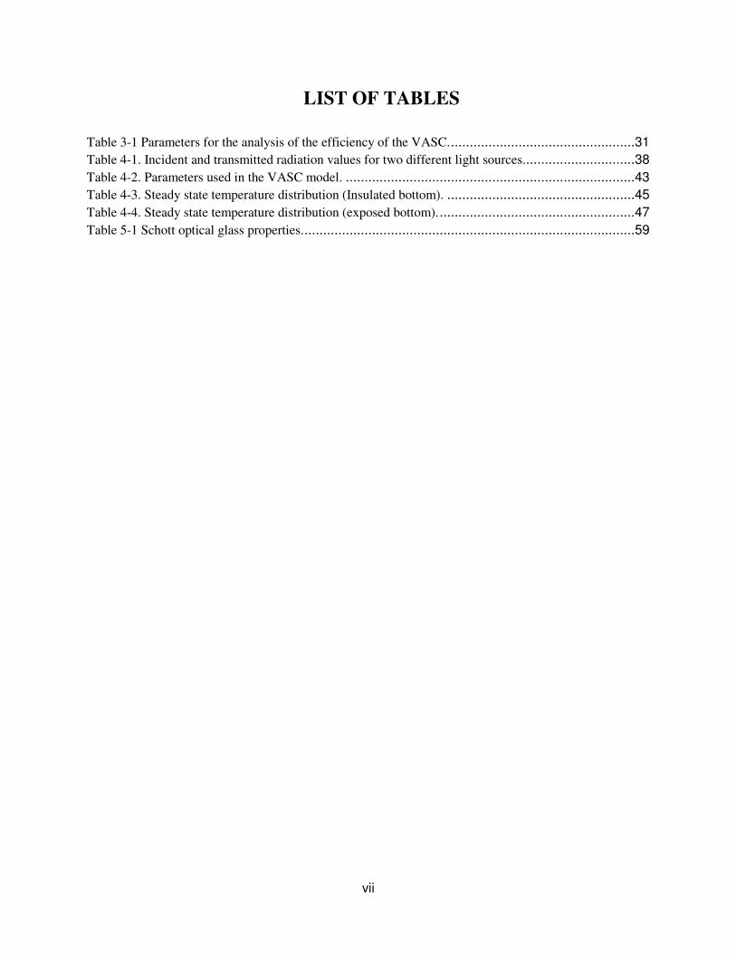
LIST OF TABLES
Table 3-1 Parameters for the analysis of the efficiency of the VASC. .................................................31
Table 4-1. Incident and transmitted radiation values for two different light sources. .............................38
Table 4-2. Parameters used in the VASC model. .............................................................................43
Table 4-3. Steady state temperature distribution (Insulated bottom). ..................................................45
Table 4-4. Steady state temperature distribution (exposed bottom). ....................................................47
Table 5-1 Schott optical glass properties. ........................................................................................59
viii
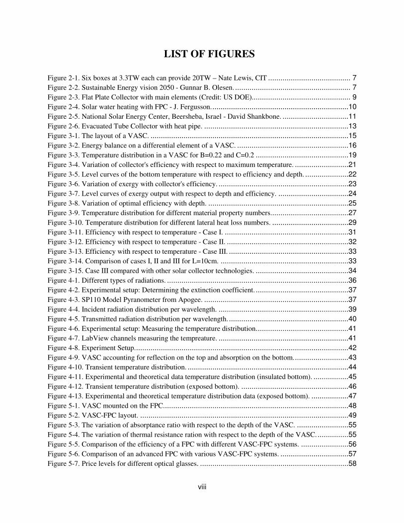
LIST OF FIGURES
Figure 2-1. Six boxes at 3.3TW each can provide 20TW – Nate Lewis, CIT ........................................ 7
Figure 2-2. Sustainable Energy vision 2050 - Gunnar B. Olesen. ........................................................ 7
Figure 2-3. Flat Plate Collector with main elements (Credit: US DOE). ............................................... 9
Figure 2-4. Solar water heating with FPC - J. Fergusson. ..................................................................10
Figure 2-5. National Solar Energy Center, Beersheba, Israel - David Shankbone. ................................11
Figure 2-6. Evacuated Tube Collector with heat pipe. ......................................................................13
Figure 3-1. The layout of a VASC. ................................................................................................15
Figure 3-2. Energy balance on a differential element of a VASC. ......................................................16
Figure 3-3. Temperature distribution in a VASC for B=0.22 and C=0.2 .............................................19
Figure 3-4. Variation of collector's efficiency with respect to maximum temperature. ..........................21
Figure 3-5. Level curves of the bottom temperature with respect to efficiency and depth. .....................22
Figure 3-6. Variation of exergy with collector's efficiency. ...............................................................23
Figure 3-7. Level curves of exergy output with respect to depth and efficiency. ..................................24
Figure 3-8. Variation of optimal efficiency with depth. ....................................................................25
Figure 3-9. Temperature distribution for different material property numbers. .....................................27
Figure 3-10. Temperature distribution for different lateral heat loss numbers. .....................................29
Figure 3-11. Efficiency with respect to temperature - Case I. ............................................................31
Figure 3-12. Efficiency with respect to temperature - Case II. ...........................................................32
Figure 3-13. Efficiency with respect to temperature - Case III. ..........................................................33
Figure 3-14. Comparison of cases I, II and III for L=10cm. ..............................................................33
Figure 3-15. Case III compared with other solar collector technologies. .............................................34
Figure 4-1. Different types of radiations. ........................................................................................36
Figure 4-2. Experimental setup: Determining the extinction coefficient. .............................................37
Figure 4-3. SP110 Model Pyranometer from Apogee. ......................................................................37
Figure 4-4. Incident radiation distribution per wavelength. ...............................................................39
Figure 4-5. Transmitted radiation distribution per wavelength. ..........................................................40
Figure 4-6. Experimental setup: Measuring the temperature distribution. ............................................41
Figure 4-7. LabView channels measuring the tempreature. ...............................................................41
Figure 4-8. Experiment Setup. .......................................................................................................42
Figure 4-9. VASC accounting for reflection on the top and absorption on the bottom. ..........................43
Figure 4-10. Transient temperature distribution. ..............................................................................44
Figure 4-11. Experimental and theoretical data temperature distribution (insulated bottom). .................45
Figure 4-12. Transient temperature distribution (exposed bottom). ....................................................46
Figure 4-13. Experimental and theoretical temperature distribution data (exposed bottom). ..................47
Figure 5-1. VASC mounted on the FPC. .........................................................................................48
Figure 5-2. VASC-FPC layout. .....................................................................................................49
Figure 5-3. The variation of absorptance ratio with respect to the depth of the VASC. .........................55
Figure 5-4. The variation of thermal resistance ration with respect to the depth of the VASC. ...............55
Figure 5-5. Comparison of the efficiency of a FPC with different VASC-FPC systems. .......................56
Figure 5-6. Comparison of an advanced FPC with various VASC-FPC systems. .................................57
Figure 5-7. Price levels for different optical glasses. ........................................................................58
ix
ABSTRACT
In a continuing effort to advance the use of solar energy and to improve the efficiency of
existing technologies, a new type of solar energy collector is presented. This method builds upon
the principles of a natural phenomenon found in solar ponds and the principles of common flat
plate collector (FPC). This type of collector, made out of a semitransparent material, was given
the name of a Volumetric Absorption Solar Collector.
A model for a Volumetric Absorption Solar Collector (VASC) accounting for lateral heat
losses has been developed and it has been experimentally validated. The model can be used to
determine the collector performance, assuming one-dimensional heat conduction and steady state
operating conditions. It is based on several dimensionless numbers, each of them having a clear
physical significance and playing a key role in the analysis of the collector. Preliminary results
suggest that with a radiation of 1000 W/m2, it is possible to obtain temperatures above 100oC
using a glass rod collector of 15 cm diameter and 15 cm length while extracting 200 W/m2.
The use of a VASC in conjunction with a FPC is one of the feasible applications of the
VASC. This joint system was analyzed and the results showed the possibility of increasing the
efficiency of a common FPC by a factor of 3 for temperatures around 100oC. Other potential
applications as well as suggestions to improve the performance of the VASC are also presented
in this work.
1
CHAPTER ONE
1 INTRODUCTION AND MOTIVATION
Energy has always been one of the world’s most important and valuable commodities.
This is all the more evident as energy is becoming an integral part of people’s everyday lives.
The availability of modern day energy allows the use of the increase of the level of comfort in
homes through heating, ventilation and air conditioning, and the access to medical care. In
addition, agriculture, construction, transportation, computing, telecommunications, and many
other essential activities would not be possible without access to energy. Undoubtedly, energy is
not just an accessory, it is essential in order to survive. Today, this statement is more applicable
than it has ever been due to several reasons that will be presented in detail below such as the
increase in energy needs, unsure security of supply and its economic consequences and the
general concern about climate change.
According to The World Energy Outlook 2009 [1], the global energy demand grew by
66% over the past 30 years. An increase of this scale or higher should be expected for the
forthcoming years. The global population is expected to grow to almost 9 billion by the year of
2030 and the standards of living for many people in developing countries are expected to
increase. The industrial development itself is expected to grow even faster than ever and, in
addition, an increasing shortage of fresh water will call for energy-intensive desalination plants,
and in the longer term hydrogen production for transport purposes will need large amounts of
electricity and/or high temperature heat. All of these events will lead to increased energy
consumption overall and in particular a doubling of electricity consumptions by the year of 2030
[1].
The security of supply and its consequences to the economy is another factor that make
energy the world’s most controversial and prestigious commodity. In the winter of 1973, the
Egyptian army raged the Suez Canal, causing an international oil supply crisis, and for the first
time oil proved itself to be a threatening weapon. Immediately after, the prices of crude oil were
raised by 70% by the Organizations of Petroleum Exporting Countries (OPEC) [2]. This incident

2
led countries to realize how vulnerable they are to interrupted deliveries of traditional fossil fuels
and their ever increasing prices. Historical data proves that there is a close relationship between
the availability of energy resources and the health of economic activities. This is confirmed by
the lack of vibrant economies in the developing nations of the world, which is mainly due to the
lack or misuse of energy resources. Since the fossil fuels reserves are exhaustible, the price of
these fuels will continue to increase as the reserves are decreased. It can be expected that at one
point the fossil fuels will be unaffordable, which will have a significant negative impact on world
economies.
Finally, increased awareness of environmental problems such as acid rain, stratospheric
ozone depletion, and the global climate change has led decision makers, media and the public to
realize that the use of fossil fuels, which contribute most to these environmental problems, must
be reduced and replaced by low-emission or zero-emission sources of energy. The daily
consumption of oil is estimated at 85 million barrels today but expected to increase to 123
million barrels per day by the year of 2025[3]. With this increase of consumption, it can be
expected that the pollution will be much greater. In light of this, it is critical that an immediate
plan of action be taken to counter these environmental problems and to insure a sustainable
development, which is a development that meets the needs of the present without compromising
the ability of future generations to meet their own needs, and to insure a sustainable planet,
which is an environment free of life threatening pollution.
Policies must be put in place to ensure that energy consumption to satisfy today’s needs
does not affect tomorrow’s generation access to the energy resources. One of the ways this can
be done is by improving the efficiency of today’s energy consuming equipment and to adopt
what is now known as the ‘fifth fuel’[4]. The fifth fuel is another word for conservation, energy
efficiency, energy productivity or energy ingenuity. It is indeed a fuel that has a long term impact
on the overall fuel consumption. The other four fuels are coal, petroleum, nuclear and alternative
energy. However, it should be pointed out that the adoption of the fifth fuel requires intensive
studies, investment in research and in educating energy consumers. Another way to achieve
economic and environmental sustainability is to increase the use of clean alternative sources of
energy, the most promising of which is solar energy.
Different technologies have been developed over the years to harness the energy from the
sun. Most of this energy is used for heating applications, water desalination, and electricity
3
production. This work proposes a method of collecting solar energy using a semitransparent solid
medium that was given the name of Volumetric Absorption Solar Collector (VASC) [5]. In this
work, a model of the VASC has been developed and experimentally validated. The model is
based on several dimensionless numbers, each of them having a clear physical significance and
playing a key role in the analysis of the collector and the determination of the collector’s
performance. Before presenting the model and results, it is useful to review some of the existing
solar energy collection technologies, and the development of solar energy throughout history.
4
CHAPTER TWO
2 HISTORY AND REVIEW OF SOLAR ENERGY
TECHNOLOGIES
2.1 History of Solar Energy
The idea of harnessing energy from the sun in order to perform useful work has been
around since prehistory. The first recorded attempt to use solar energy was by the Greek
philosopher Socrates (470-399) who might have taught how to correctly orient dwellings in order
to have houses which were cool in summer and warm in winter; this is recorded in Socrates
memorabilia by Xenophon [6]. Legend also has it that in the year of 212 B.C. the physicist
Archimedes attempted to develop a method to burn the Roman fleet by using a concave mirror to
reflect all the incoming radiation on one ship. Whether or not the Greek scientist’s attempt
actually succeeded is a subject of controversy. It is also suggested that in ancient Mesopotamia,
the priests may have used highly polished bowls as parabolic mirrors to ignite fires on the altar.
What is certain is that around the year of 1000 AD, the work of the Egyptian mathematician Ibn
al-Haytham (965-1039AD) in optics catapulted the developments in concave mirrors (burning
mirrors). Around the year of 1515 AD, the Italian artist and scientist Leornardo Da Vinci
proposed to build a large 6.5-kilometer diameter concave mirror to focus the sunlight and
provide enough heat for commercial enterprises. The focal point was located at a distance of 4
meters. He conducted experiments to validate his design using large silver-vanished concave
mirrors [7].
In the late 1700, Germans were able to build large focusing mirrors that were used to
burn objects at a distance of 10 meters. The mirrors had the capacity of focusing the sun rays to
an area of less than 30 square centimeters. The focused rays had enough heat to melt Copper ores
in seconds [7].
5
Solar energy technologies saw major advances in the late 19th century and early 20th
century. In 1878, Augustin Mouchot presented a solar device at the Universal Exposition in
Paris. He had built a prototype a decade before that led Napoleon III to fund his project. This
device had a form of a cone with a total reflecting surface area of 5 m2. A boiler was placed
along the axis of the device and provided steam to drive a 0.5 hp engine at 80 rpm.
In 1880, John Ericsson built an engine to run on solar heat. The driving force from the pistons
could push the flywheel at the speed of 400 rpm [7].
The largest solar undertaking in the early 20th century was accomplished by Frank
Shuman in 1914, in Egypt by building the largest pumping plant in the world. This solar-
powered plant produced approximately 45kW continuously for a 5 hour period. It was
abandoned due to the immediate availability of cheaper fuel. His original plan was to build
50,000 km2 in the Sahara desert. If today’s technology was to be used, this surface could provide
as much as 2.5 TW of electricity [7].
The years that followed, the world of energy was dominated by fossil fuel until the year
of 1975 when a subtle rebirth of solar energy was experienced. In the summer of 1975, President
Jimmy Carter held the first ever press conference on the rooftop of the White House. At this
occasion, a new solar heating system, worth $28,000, was inaugurated. President Carter made it
clear that the system would pay of itself in less than a decade. He made a promise that the United
States would get 20 percent of its total energy needs from solar by the end of the 20th century and
also promised to spend $1B to get it started. In the year of 1980, President Carter lost his
reelection campaign to Ronald Reagan who ended all of Carter’s solar energy promises. In the
year of 2009, solar energy constituted less than 1.5 percent of the U.S. energy supply; no
advances had been made since the Carter’s times [8].
Today, more than any other time in history, leaders worldwide have started to realize the
inevitable need to put more effort in developing solar energy technologies along with other
renewable sources of energy. President Barack Obama, in his effort to promote the renewable
sources of energy, has said that “the nation that leads the world in creating new energy sources
will be the nation that leads the twenty-first-century global economy.” And in his most recent
state of the union address, he highlighted his energy vision when he said: “I will not run away
from the hope of renewable energies”. President Hu Jintao of China also said that “China must
seize the preemptive opportunities in the new round of the global energy revolution,” also
6
referring to the rise of renewable energies [8]. The European Union has a 20 percent renewable
energy goal by the year of 2020 and Germany in particular has set a new target to increase the
renewables’s share of electricity from 17 percent to 35 percent by the year of 2020. Also
referring to the renewables, David Cameron of Great Britain has promised the most dramatic
change in Britain’s energy policy. From these statements from the world’s most prominent
leaders, it is fair to say that the train of renewable energies has left the station [8].
2.2 Viability of Solar Energy
It’s common to wonder if the solar energy could ever be enough to satisfy all the global
energy needs. To remove all doubt, it may be useful to present some of the facts regarding the
sun. The sun is a large sphere located 1.5x10¹¹ meters away from the earth with a diameter of
1.39x10⁹ meters. The overall temperature of the sun is estimated at 5762 K, although it get as
high as 40x106 K at the sun’s core [9]. The sun radiates its energy in all directions and only a
small portion of it is intercepted by the earth. Even though this portion is small, estimated at
1.7x10¹⁴ kW, 30 minutes of solar radiation befalling the earth contains the same amount of
energy equal to the world energy demand for one year [9]. Nate Lewis of the California Institute
of Technology proved that there is enough radiation from the sun to meet all energy needs on
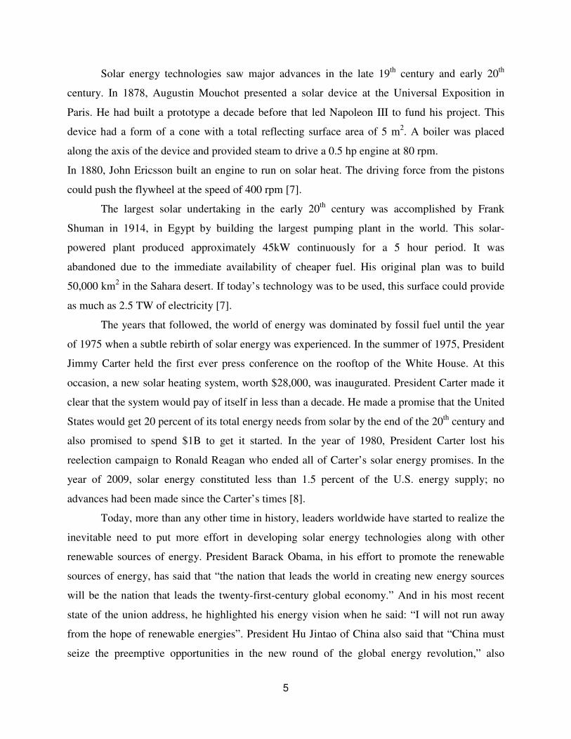
planet earth, which are estimated at 2 kW per person [10]. By selecting 6 rectangular spaces on
earth with a high solar radiation like those shown in figure 2-1, which are mostly deserts and
unexploited, and applying a conversion efficiency of 10%, it is possible to collect as much as 20
TW of electrical power, which is enough to satisfy the energy needs of 10 billion people, the
projected world population in the year of 2050.
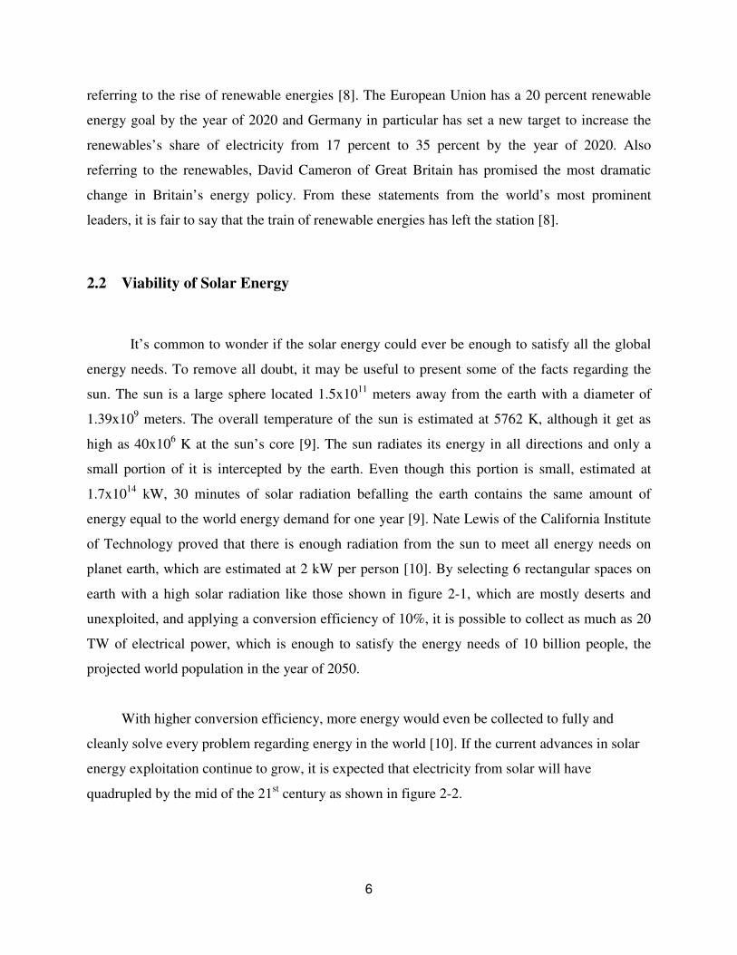
With higher conversion efficiency, more energy would even be collected to fully and
cleanly solve every problem regarding energy in the world [10]. If the current advances in solar
energy exploitation continue to grow, it is expected that electricity from solar will have
quadrupled by the mid of the 21st century as shown in figure 2-2.
7
Figure 2-1. Six boxes at 3.3TW each can provide 20TW – Nate Lewis, CIT
Figure 2-2. Sustainable Energy vision 2050 - Gunnar B. Olesen.
8
2.3 Solar Energy Technologies
In the recent years, solar power technology has seen important improvements, both in
solar heating technologies and solar photovoltaic technologies. This discussion will mainly focus
on solar heating technologies. There are two criterions commonly used to classify solar heating
technologies: the solar radiation received per surface area of the collector distinguishes
concentrating collectors from non-concentrating collectors; the tracking of the sun distinguishes
stationary collectors from sun-tracking collectors. Non-concentrating collectors only absorb solar
radiation that is intercepted by their surface area. Examples of these include flat plate collectors,
evacuated tube collectors, solar fences, etc. Concentrating collectors receive solar radiation and
redirect it on a point-focus to heat a working fluid. The working fluid, also known as the
transport medium, which can be water, oil or air runs through the collector and receives the
energy accumulated in the collector. This energy is then transported to a thermal energy storage
for later use or can be directly used for water heating or space heating applications and several
other applications. Examples of this category include parabolic trough systems, parabolic dish,
power towers, etc… [11]. Both concentrating and non-concentrating collectors can either be
stationary or sun-tracking.
The list of solar heating technologies is long. Each technology has also been a subject to
important improvements over the years. This brief discussion will highlight three of the major
solar heating technologies, namely flat plate collectors (FPC), parabolic trough collectors (PTC)
and evacuated tube collectors (ETC). Also presented, is a discussion of another unpopular but
important solar heat collecting technology, the solar pond, which is closely related to the VASC
presented in this work.
2.3.1 Flat Plate Collectors
Flat plate collectors are a very widely used type of collectors. They are mostly used for
low temperature applications up to 100oC. Recent advances have been made in improving
insulation materials and special coatings that allow FPCs to reach temperatures of 200oC or
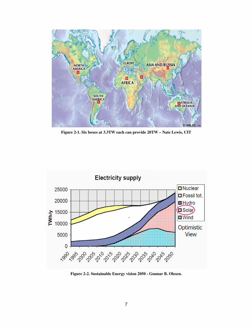
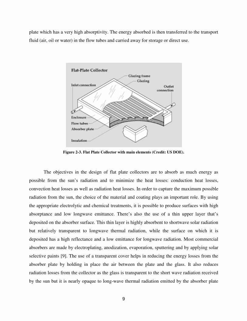
higher. The main parts of a FPC include the flow tubes, the absorber plate and glazing (figure 2-
3). Solar radiation passes through the semitransparent cover and is absorbed by the absorber
9
plate which has a very high absorptivity. The energy absorbed is then transferred to the transport
fluid (air, oil or water) in the flow tubes and carried away for storage or direct use.
Figure 2-3. Flat Plate Collector with main elements (Credit: US DOE).
The objectives in the design of flat plate collectors are to absorb as much energy as
possible from the sun’s radiation and to minimize the heat losses: conduction heat losses,
convection heat losses as well as radiation heat losses. In order to capture the maximum possible
radiation from the sun, the choice of the material and coating plays an important role. By using
the appropriate electrolytic and chemical treatments, it is possible to produce surfaces with high
absorptance and low longwave emittance. There’s also the use of a thin upper layer that’s
deposited on the absorber surface. This thin layer is highly absorbent to shortwave solar radiation
but relatively transparent to longwave thermal radiation, while the surface on which it is
deposited has a high reflectance and a low emittance for longwave radiation. Most commercial
absorbers are made by electroplating, anodization, evaporation, sputtering and by applying solar
selective paints [9]. The use of a transparent cover helps in reducing the energy losses from the
absorber plate by holding in place the air between the plate and the glass. It also reduces
radiation losses from the collector as the glass is transparent to the short wave radiation received
by the sun but it is nearly opaque to long-wave thermal radiation emitted by the absorber plate
10
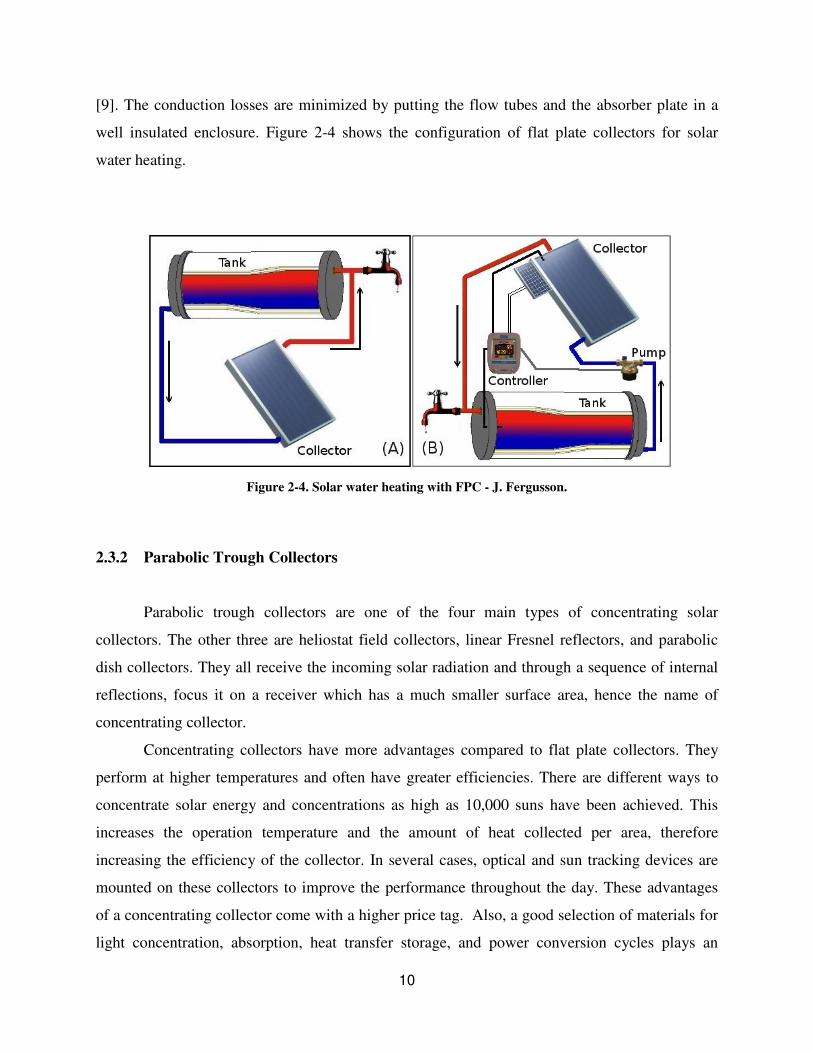
[9]. The conduction losses are minimized by putting the flow tubes and the absorber plate in a
well insulated enclosure. Figure 2-4 shows the configuration of flat plate collectors for solar
water heating.
Figure 2-4. Solar water heating with FPC - J. Fergusson.
2.3.2 Parabolic Trough Collectors
Parabolic trough collectors are one of the four main types of concentrating solar
collectors. The other three are heliostat field collectors, linear Fresnel reflectors, and parabolic
dish collectors. They all receive the incoming solar radiation and through a sequence of internal
reflections, focus it on a receiver which has a much smaller surface area, hence the name of
concentrating collector.
Concentrating collectors have more advantages compared to flat plate collectors. They
perform at higher temperatures and often have greater efficiencies. There are different ways to
concentrate solar energy and concentrations as high as 10,000 suns have been achieved. This
increases the operation temperature and the amount of heat collected per area, therefore
increasing the efficiency of the collector. In several cases, optical and sun tracking devices are
mounted on these collectors to improve the performance throughout the day. These advantages
of a concentrating collector come with a higher price tag. Also, a good selection of materials for
light concentration, absorption, heat transfer storage, and power conversion cycles plays an
11
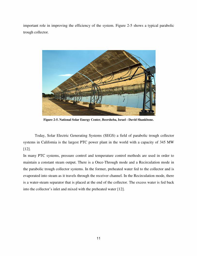
important role in improving the efficiency of the system. Figure 2-5 shows a typical parabolic
trough collector.
Figure 2-5. National Solar Energy Center, Beersheba, Israel - David Shankbone.
Today, Solar Electric Generating Systems (SEGS) a field of parabolic trough collector
systems in California is the largest PTC power plant in the world with a capacity of 345 MW
[12].
In many PTC systems, pressure control and temperature control methods are used in order to
maintain a constant steam output. There is a Once-Through mode and a Recirculation mode in
the parabolic trough collector systems. In the former, preheated water fed to the collector and is
evaporated into steam as it travels through the receiver channel. In the Recirculation mode, there
is a water-steam separator that is placed at the end of the collector. The excess water is fed back
into the collector’s inlet and mixed with the preheated water [12].
12
2.3.3 Evacuated Tube Collectors
The evacuated tube solar collector (ETC) technology is another popular solar energy
collecting technology. In fact, in some areas of the globe, the ETC technology dominates the
industry of solar water heating. When compared to flat plate collectors, ETC have a better
thermal efficiency at temperatures above 80°C [13]. The ETC also presents the advantage of a
much steadier efficiency as the temperature increases. It has experimentally been shown that
when the average temperature is increased from 50 to 90°C, the efficiency of the ETC only
decreased from 60 to 50% [14]. This allows for the use of ETC for high temperature
applications, such as power generation at a small expense of the thermal efficiency. He W. et al
have proposed to use the ETC in conjunction with thermoelectric modules to produce electricity
in addition to heating water [15].
There are two types of evacuated tube collectors: single-phase evacuated tube collectors
and two-phase evacuated tube collectors. The evacuated tube designed for single-phase is made
of two concentric borosilicate glass tubes sealed at one end. The space between the two tubes is
evacuated to minimize the conduction and convection losses. Radiation heat losses are
minimized by a selective coating applied to the outer surface of the inner tube. This coating also
contributes to the maximization of heat absorption. The heat absorbed by the inner tube warms
up the water (working fluid) which develops a buoyant flow up the tube and is displaced by an
inflow of cold water from the storage [16].
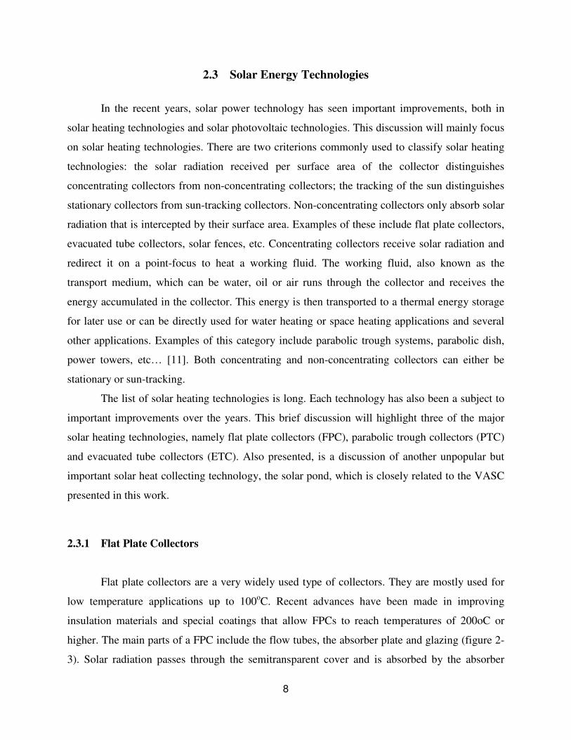
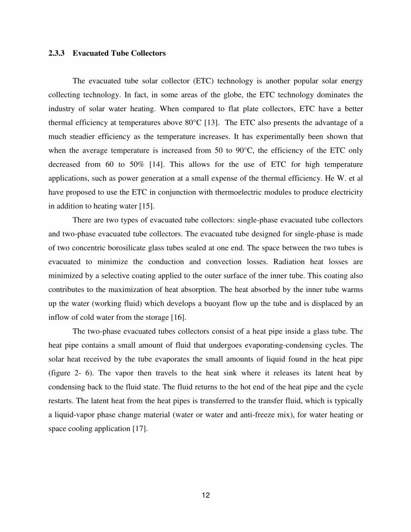
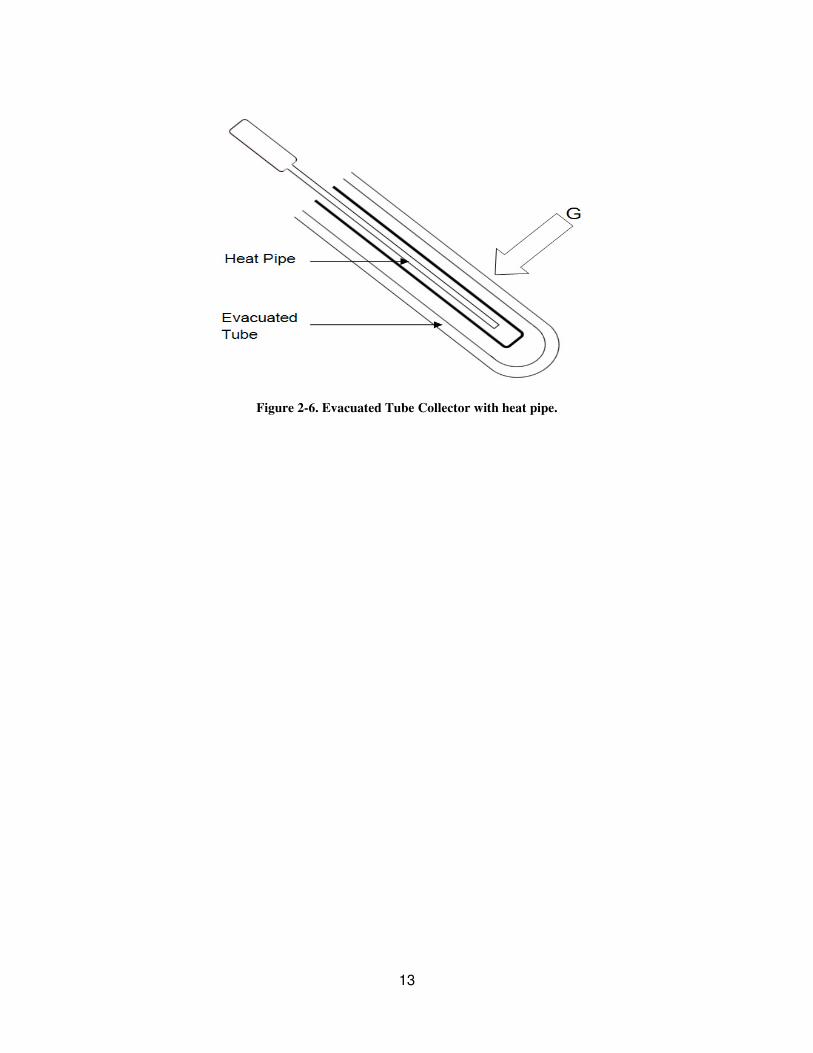
The two-phase evacuated tubes collectors consist of a heat pipe inside a glass tube. The
heat pipe contains a small amount of fluid that undergoes evaporating-condensing cycles. The
solar heat received by the tube evaporates the small amounts of liquid found in the heat pipe
(figure 2- 6). The vapor then travels to the heat sink where it releases its latent heat by
condensing back to the fluid state. The fluid returns to the hot end of the heat pipe and the cycle
restarts. The latent heat from the heat pipes is transferred to the transfer fluid, which is typically
a liquid-vapor phase change material (water or water and anti-freeze mix), for water heating or
space cooling application [17].
13
Figure 2-6. Evacuated Tube Collector with heat pipe.
14
CHAPTER THREE
3 THE VOLUMETRIC ABSORPTION SOLAR COLLECTOR:
THEORETICAL ANALYSIS
3.1 Introduction
A Volumetric Solar Absorption (VASC) is a semitransparent solid medium used to
collect and store solar radiation and deliver it as heat transfer [18-20]. Several factors influence
the temperatures that can be reached within the VASC. These factors vary from the amount of
solar radiation received to the size of the collector and the collector’s material properties. Some
VASC might have physical limitations regarding the maximum temperatures they can withstand.
This work will focus on a solid semitransparent material. The solid material has a higher
melting point and presents an advantage over liquid material for high temperature applications.
The physics of a VASC have been studied and model has been derived and implemented. The
model contains several dimensionless parameters, each of which has a clear physical
significance. The objective of this work is to determine which of these factors are critical to the
performance of the collector and ways in which the performance can be improved by varying the
dimensionless numbers.
This work is a continuation of a previous analysis of VASC model that did not take into
account lateral heat losses [18]. A perfectly insulated VASC provides the maximum achievable
temperatures in the collector and can therefore be used for comparison purposes. In practice,
even with the most efficient insulation, there are still heat losses on the sides of the collector.
This new model takes into account and studies the effect of these losses.
15
3.2 Heat Transfer Analysis
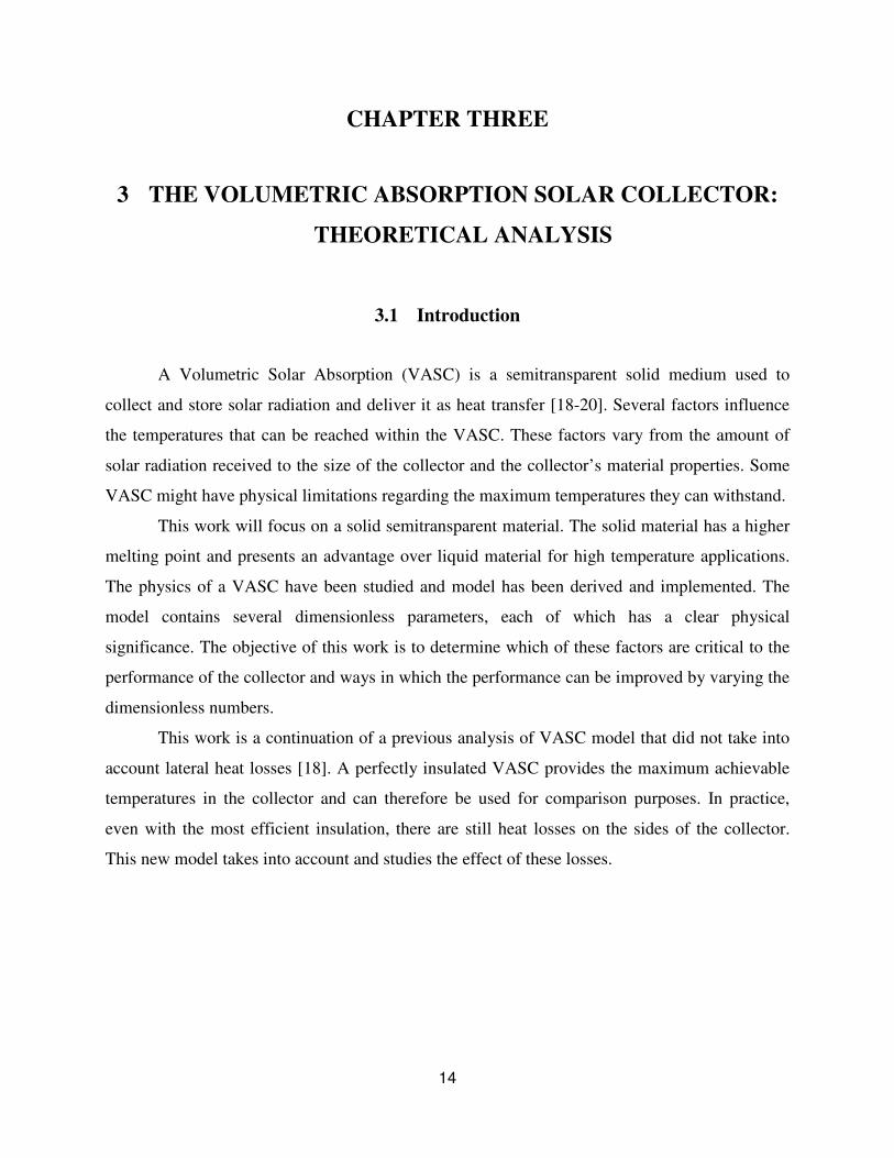
The VASC studied in this paper has a cylindrical form and is made out of a
semitransparent solid material such as glass or acrylic. The lateral surface of the cylinder is
covered by an insulating material. The top surface is exposed to incident solar radiation and the
energy is extracted from the bottom surface. Figure 3-1 shows a schematic of the VASC.
Figure 3-1. The layout of a VASC.
This model assumes steady state conditions, one dimensional heat conduction and
constant properties. It also takes into consideration lateral heat losses due to convection.
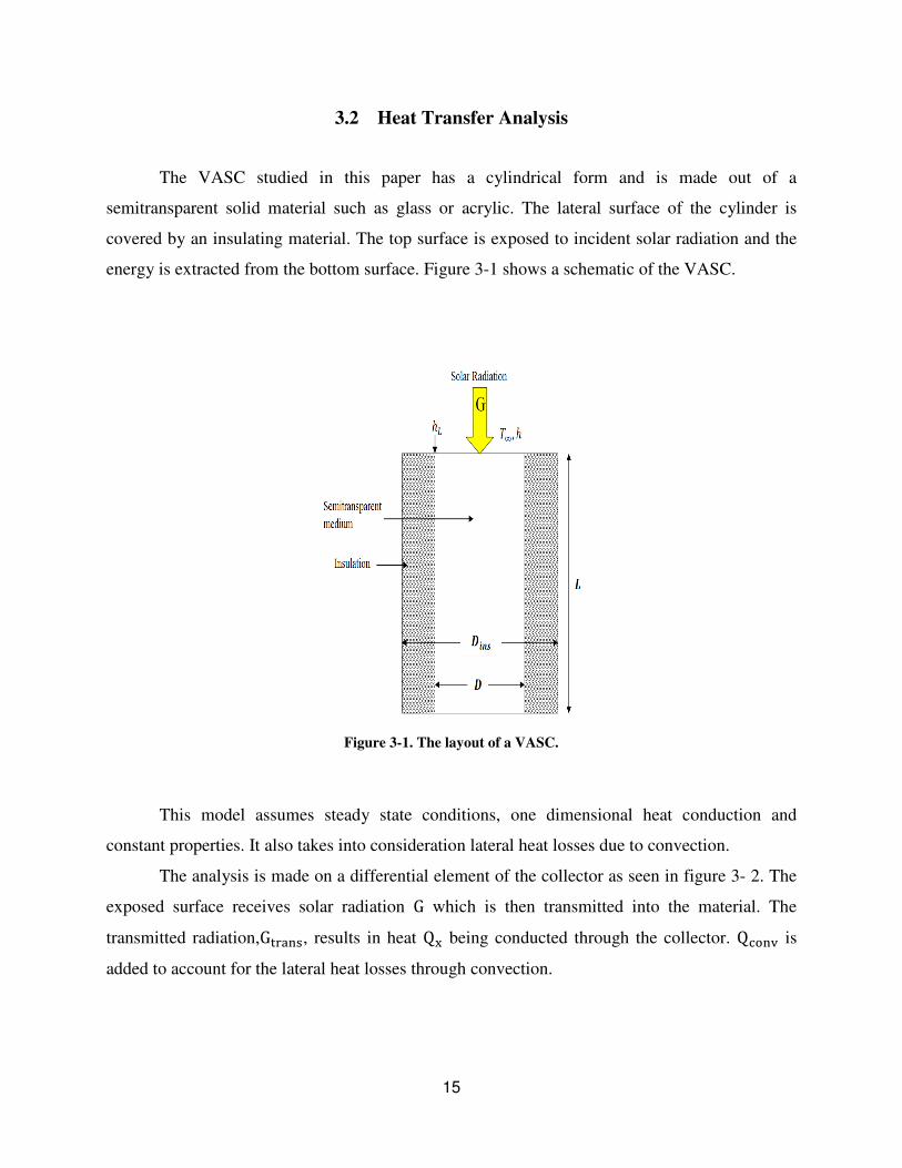
The analysis is made on a differential element of the collector as seen in figure 3- 2. The
exposed surface receives solar radiation G which is then transmitted into the material. The
transmitted radiation,G�����, results in heat Q� being conducted through the collector. Q�� is
added to account for the lateral heat losses through convection.
16
Figure 3-2. Energy balance on a differential element of a VASC.
Using the law of conservation of energy we obtain
� �� � � AT ������ � � Q�� � 0 (3-1)
Applying the Fourier’s law of conduction,
Q� � �kA� � � (3-2)
Newton’s law of cooling
Q�� � h�A��T � T∞� (3-3)
and the Beer’s law of transmissivity [21],
G����� � Q e"�� (3-4)
Equation 3-1 becomes
$� �$ % � �& e"�� � '()& *+ �T � T∞� � 0 (3-5)
17
where Q is the incident solar radiation, T is the temperature of the collector, k is the thermal
conductivity of the material, � is the material’s extinction coefficient, h� is the convection
coefficient between the material and the insulation, A� � πD- 4⁄ is the top area of the collector,
and P � πD is the perimeter.
The convection coefficient h� can be determined from the knowledge of the effective thermal
resistance R between the collector and the external medium.
R � ln4DinsD 72πkinsL % 1hAins � 1hLAL (3-6)
Rearranging (3-6), the equivalent convection coefficient is
h� � ;<(�=<>��< ?
$@>�� A <B<>�� (3-7)
where D and DC�� are the diameters of the collector and insulation respectively, kC�� is the
thermal conductivity of the insulation material, h is the convection coefficient with the external
medium.
Eq. 3-5 can be written in a non-dimensional form by dividing it by T∞�-
$θ �D$ % Ae"�D � C-�θ� 1� � 0 (3-8)
where
xD � �x (Dimensionless position) (3-9)
θ � ��∞ (Dimensionless temperature) (3-10)
A � � �&�∞ (Material property number) (3-11)
18
C- � G'(&H�$ (Lateral heat loss number) (3-12)
Eq. 3-8 is a second order ordinary differential equation with the general solution
θ � K;eJ�D % K-e"J�D � *;"J$ e"�D % 1 (3-13)
The constants K; and K- are determined by applying the appropriate boundary conditions. For
this particular case, the boundary conditions are known at xD � 0 and xD � �L.
At xD � 0, dθdxD � AB �θ� 1�
where
B � Q hT∞ (Heat loss number) (3-14)
At xD � �L
dθdxD � AOe�xP � ηR
η � QQ (Efficiency) (3-15)
Q is the energy extracted at the bottom. The efficiency η is the ratio between the extracted energy
and the incident solar radiation. The more energy extracted the greater the efficiency and the
lower the temperature of a VASC.
Applying these boundary conditions, the constants K; and K- are
K; � A�BC%A�Se�µLU C21�C2V%ηW�AC�A%B�e�µLC= 11�C2?
C�BC�A�e�µCL�C�BC%A�eµLC (3-16a)
19
K- � A�BC�A�Se�µLU C21�C2V%ηW�AC�A%B�eµLC= 11�C2?
C�BC�A�e�µLC�C�BC%A�eµLC (3-16b)
By replacing x with L in equation 3-9, a new dimensionless variable ε � �L can be
defined, called the dimensionless depth. Replacing xD with ε in equation 3-13, the resulting
equation represents the temperature of the collector’s bottom and is given by the following
identity
θX � K;eJY % K-e"JY � *;"J$ e"Y % 1 (3-17)
3.2.1 Temperature Distribution
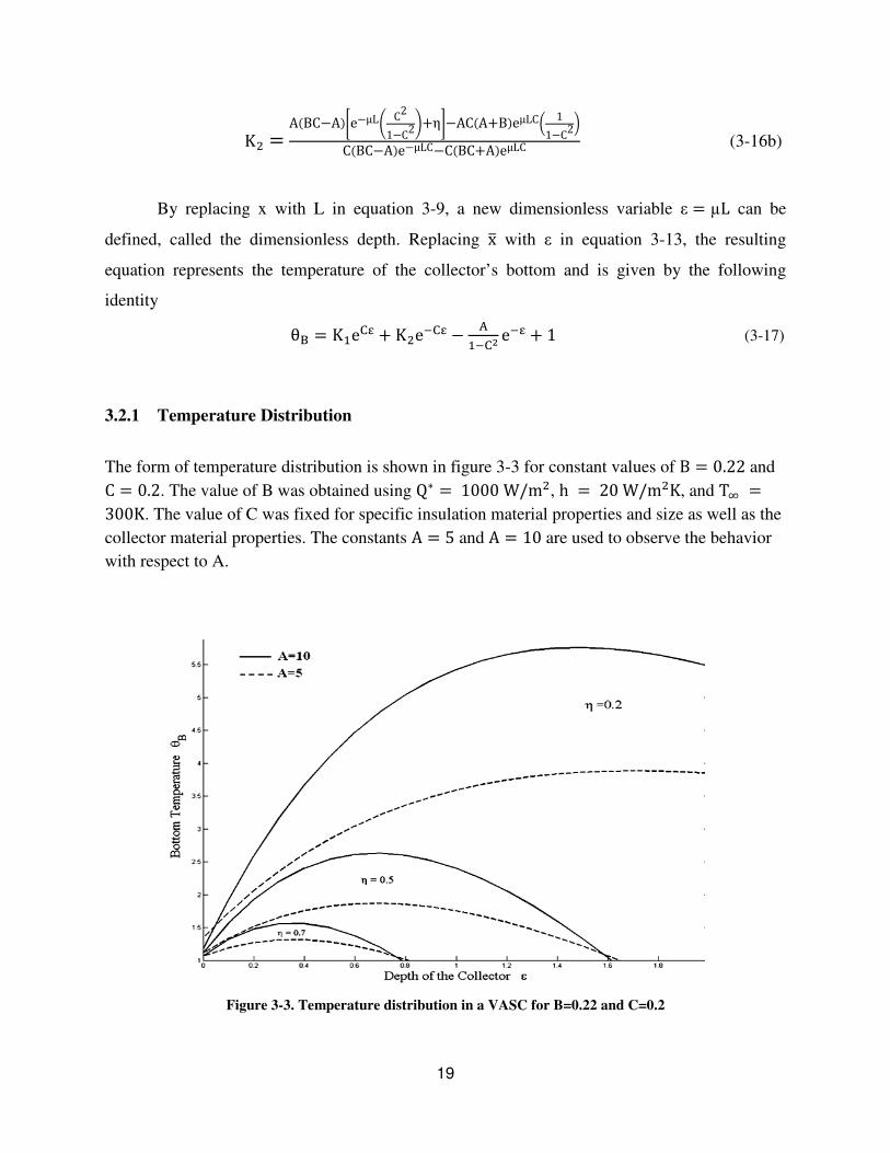
The form of temperature distribution is shown in figure 3-3 for constant values of B � 0.22 and C � 0.2. The value of B was obtained using Q � 1000 W/m-, h � 20 W/m-K, and T̂ �300K. The value of C was fixed for specific insulation material properties and size as well as the
collector material properties. The constants A � 5 and A � 10 are used to observe the behavior
with respect to A.
Figure 3-3. Temperature distribution in a VASC for B=0.22 and C=0.2
20
Figure 3-3 illustrates the variation of the collector temperature as a function of the
position (or the collector’s bottom temperature as a function of depth) for different efficiencies
and material property number. For each combination of efficiency and the group A there is a
maximum temperature. The value of ε at which θ reaches one represents the maximum depth for
which the collector can operate at the given efficiency. Observe that the maximum depth is
independent from A but is strongly dependent on the efficiency. For higher efficiencies, the
maximum depth is smaller. The depth at which the bottom temperature reaches its maximum
value also depends on the efficiency. For a constant A, the higher the efficiency the smaller the
depth needed to reach this temperature. It is also possible to see that for a constant depth, the
higher temperatures are reached with the lower efficiencies, meaning that the lesser the heat
extracted by the user the higher the temperature distribution of the collector. It may be useful to
point out that the form of this temperature distribution matches the form of the popular
volumetric solar receivers [9].
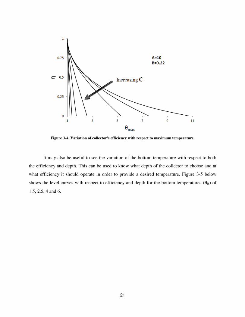
It is also important to study the effects of lateral heat losses. The material properties and
size of the collector and insulation play an important role in the determination of the lateral heat
losses. All of these properties are embodied in one non-dimensional heat loss number called C.
Small values of C result in reduced amounts of heat losses, and as shown in figure 3-4, the
maximum temperatures that can be achieved for given efficiencies get smaller as the value of C
gets bigger. In the following chapter, an analysis will be done on collectors for which the C value
is reduced to zero.
21
Figure 3-4. Variation of collector's efficiency with respect to maximum temperature.
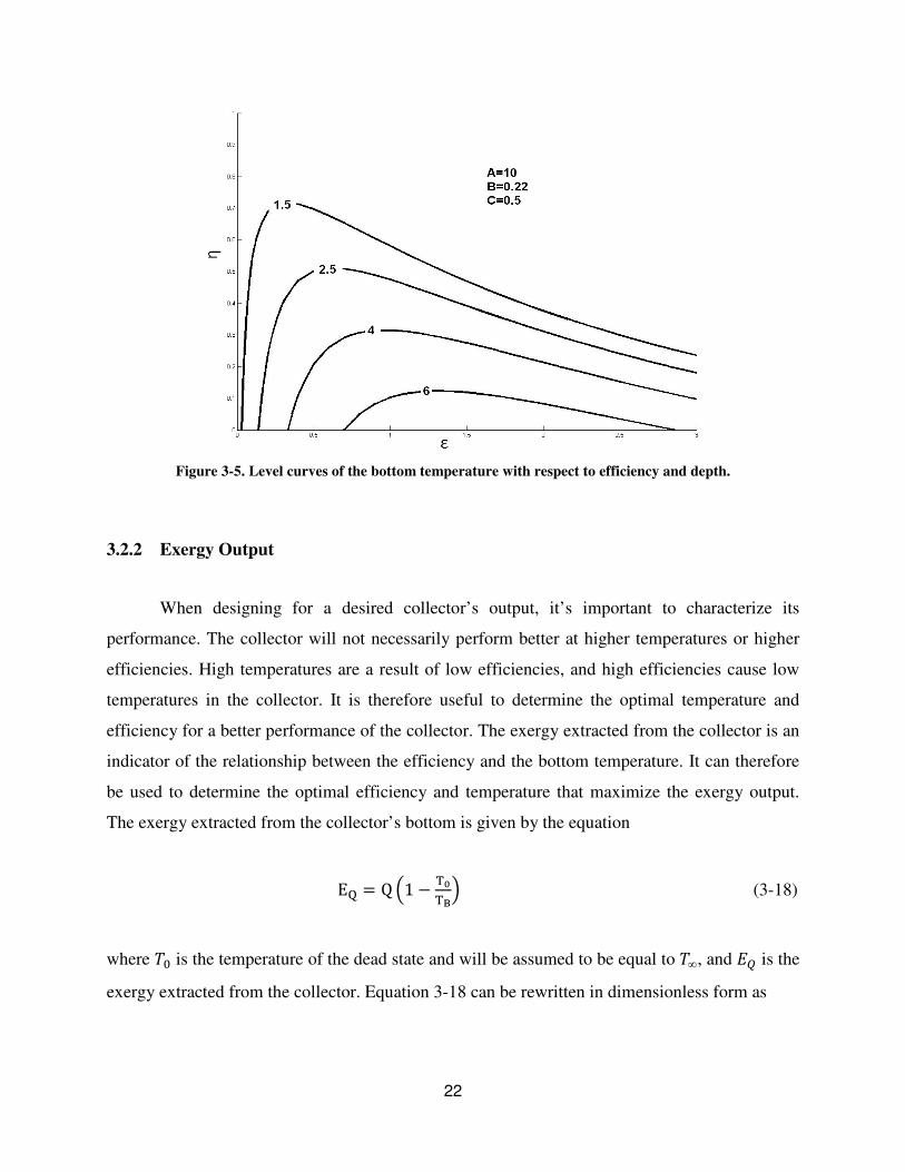
It may also be useful to see the variation of the bottom temperature with respect to both
the efficiency and depth. This can be used to know what depth of the collector to choose and at
what efficiency it should operate in order to provide a desired temperature. Figure 3-5 below
shows the level curves with respect to efficiency and depth for the bottom temperatures (θB) of
1.5, 2.5, 4 and 6.
22
Figure 3-5. Level curves of the bottom temperature with respect to efficiency and depth.
3.2.2 Exergy Output
When designing for a desired collector’s output, it’s important to characterize its
performance. The collector will not necessarily perform better at higher temperatures or higher
efficiencies. High temperatures are a result of low efficiencies, and high efficiencies cause low
temperatures in the collector. It is therefore useful to determine the optimal temperature and
efficiency for a better performance of the collector. The exergy extracted from the collector is an
indicator of the relationship between the efficiency and the bottom temperature. It can therefore
be used to determine the optimal efficiency and temperature that maximize the exergy output.
The exergy extracted from the collector’s bottom is given by the equation
E� � Q 41 � �b�c7 (3-18)
where de is the temperature of the dead state and will be assumed to be equal to d∞, and fg is the
exergy extracted from the collector. Equation 3-18 can be rewritten in dimensionless form as
23
Ξ � η 41 � ;θc7 (3-19)
where
Ξ � hi� (3-20)
j is the exergy output number and symbolizes the exergy extracted from the collector’s bottom
in a dimensionless form. It represents the fraction of the solar energy that is available to be
transformed into work. It is a function of A, B, C, k and l.
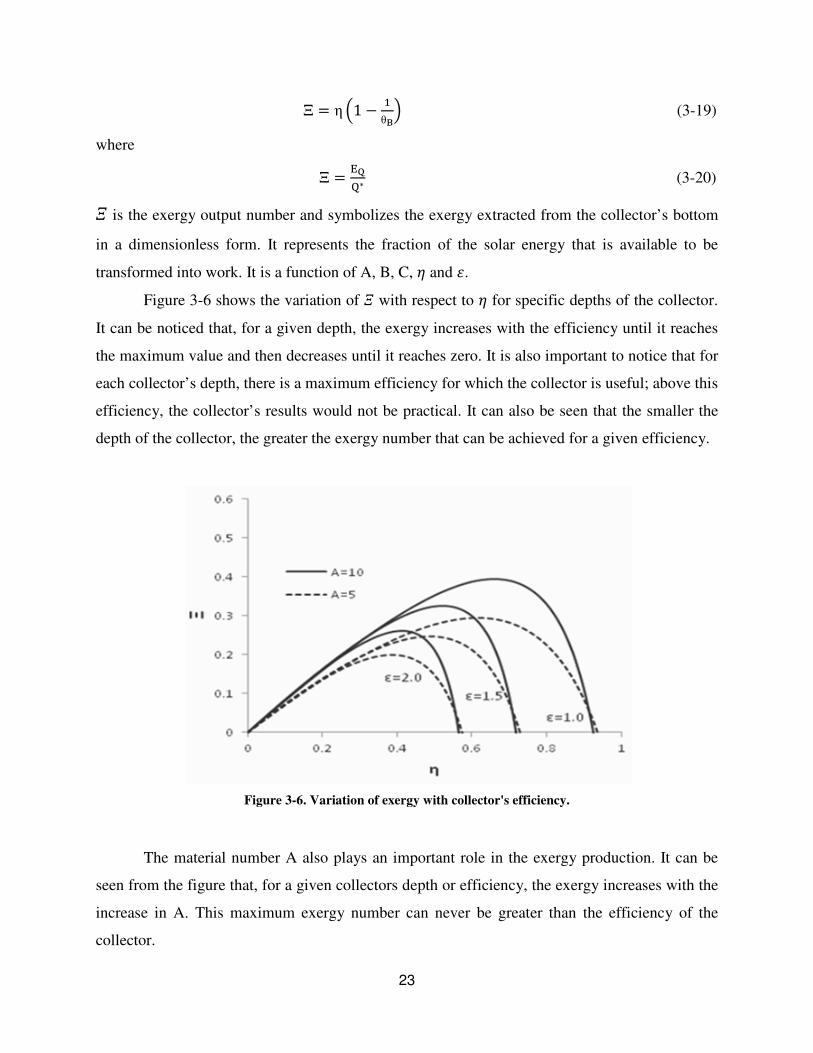
Figure 3-6 shows the variation of j with respect to k for specific depths of the collector.
It can be noticed that, for a given depth, the exergy increases with the efficiency until it reaches
the maximum value and then decreases until it reaches zero. It is also important to notice that for
each collector’s depth, there is a maximum efficiency for which the collector is useful; above this
efficiency, the collector’s results would not be practical. It can also be seen that the smaller the
depth of the collector, the greater the exergy number that can be achieved for a given efficiency.
Figure 3-6. Variation of exergy with collector's efficiency.
The material number A also plays an important role in the exergy production. It can be
seen from the figure that, for a given collectors depth or efficiency, the exergy increases with the
increase in A. This maximum exergy number can never be greater than the efficiency of the
collector.
24
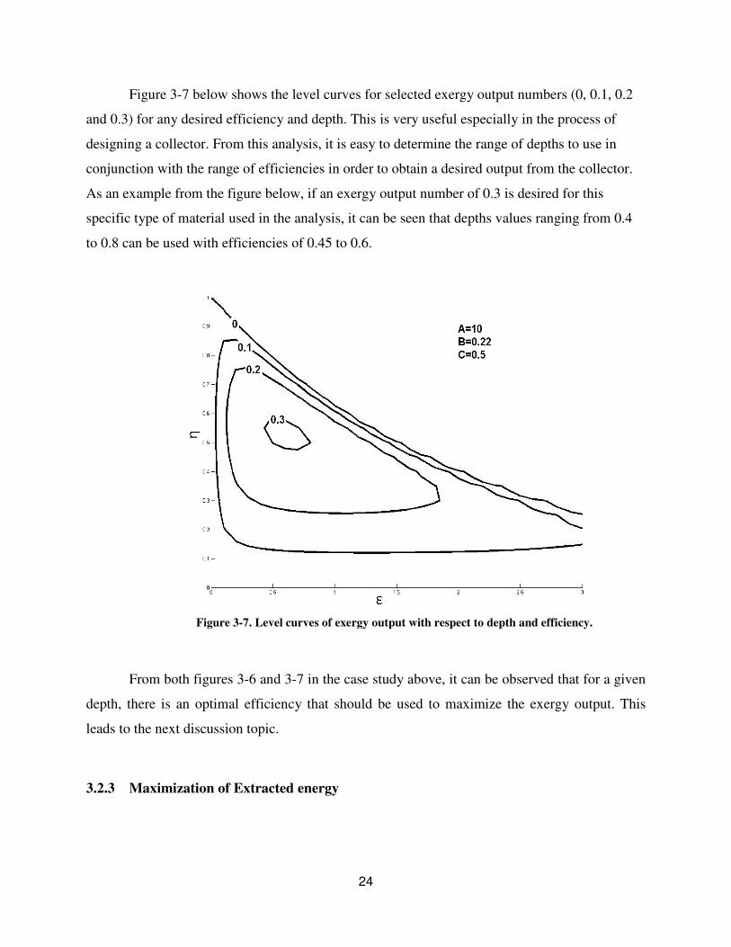
Figure 3-7 below shows the level curves for selected exergy output numbers (0, 0.1, 0.2
and 0.3) for any desired efficiency and depth. This is very useful especially in the process of
designing a collector. From this analysis, it is easy to determine the range of depths to use in
conjunction with the range of efficiencies in order to obtain a desired output from the collector.
As an example from the figure below, if an exergy output number of 0.3 is desired for this
specific type of material used in the analysis, it can be seen that depths values ranging from 0.4
to 0.8 can be used with efficiencies of 0.45 to 0.6.
Figure 3-7. Level curves of exergy output with respect to depth and efficiency.
From both figures 3-6 and 3-7 in the case study above, it can be observed that for a given
depth, there is an optimal efficiency that should be used to maximize the exergy output. This
leads to the next discussion topic.
3.2.3 Maximization of Extracted energy
25
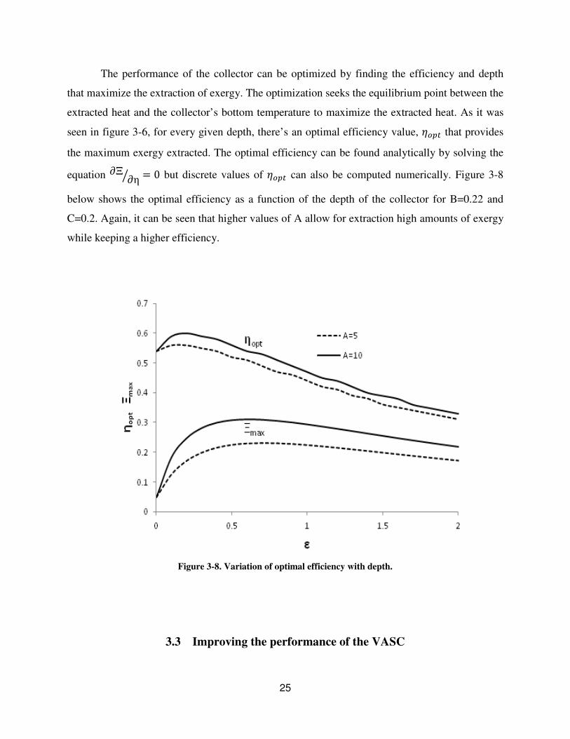
The performance of the collector can be optimized by finding the efficiency and depth
that maximize the extraction of exergy. The optimization seeks the equilibrium point between the
extracted heat and the collector’s bottom temperature to maximize the extracted heat. As it was
seen in figure 3-6, for every given depth, there’s an optimal efficiency value, kmno that provides
the maximum exergy extracted. The optimal efficiency can be found analytically by solving the
equation ∂Ξ ∂ηq � 0 but discrete values of kmno can also be computed numerically. Figure 3-8
below shows the optimal efficiency as a function of the depth of the collector for B=0.22 and
C=0.2. Again, it can be seen that higher values of A allow for extraction high amounts of exergy
while keeping a higher efficiency.
Figure 3-8. Variation of optimal efficiency with depth.
3.3 Improving the performance of the VASC
26
3.3.1 Optimizing System’s Parameters
It has been shown that a number of factors play key roles in the performance of a
volumetric absorption solar collector. The most important of these factors are: the dimensionless
number A, which is a material property number, the dimensionless number B, which is a heat
loss number and the dimensionless number C, which is a lateral heat losses number.
� The material property number, A (Eq. 3-11)
r � s tud̂
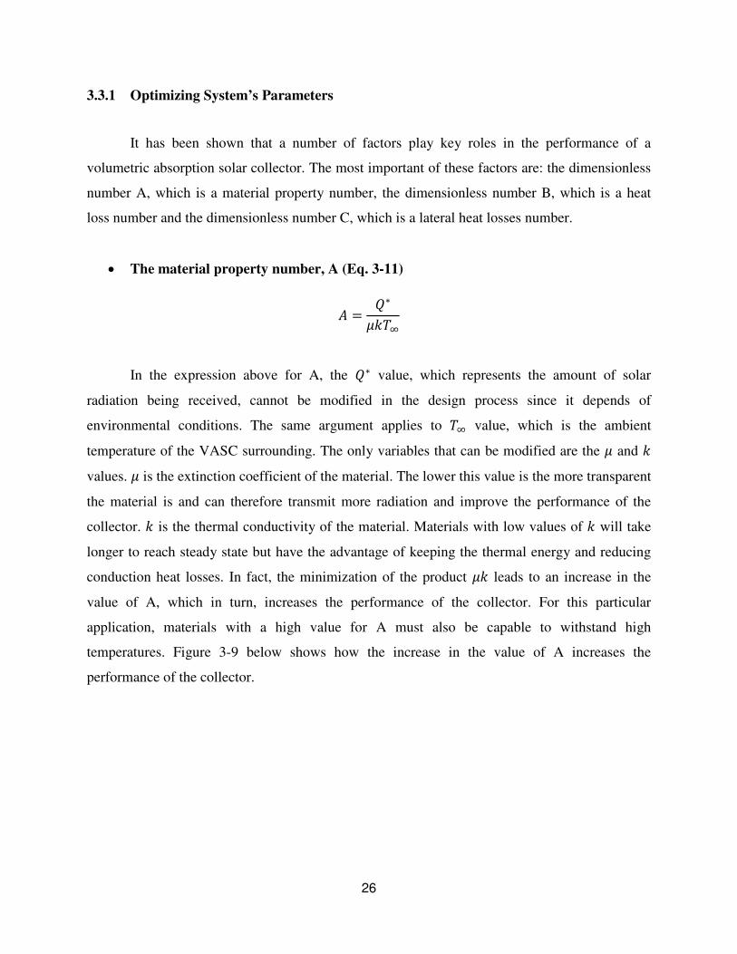
In the expression above for A, the s value, which represents the amount of solar
radiation being received, cannot be modified in the design process since it depends of
environmental conditions. The same argument applies to d̂ value, which is the ambient
temperature of the VASC surrounding. The only variables that can be modified are the t and u
values. t is the extinction coefficient of the material. The lower this value is the more transparent
the material is and can therefore transmit more radiation and improve the performance of the
collector. u is the thermal conductivity of the material. Materials with low values of u will take
longer to reach steady state but have the advantage of keeping the thermal energy and reducing
conduction heat losses. In fact, the minimization of the product tu leads to an increase in the
value of A, which in turn, increases the performance of the collector. For this particular
application, materials with a high value for A must also be capable to withstand high
temperatures. Figure 3-9 below shows how the increase in the value of A increases the
performance of the collector.
27
Figure 3-9. Temperature distribution for different material property numbers.
� The heat loss number B (Eq. 3-14)
v � s wd̂
This heat loss number does not play a major role in the optimization of the performance
of the volumetric absorption solar collector. The solar radiation and ambient temperature cannot
be freely modified in the design since they depend on the weather conditions. The convection
coefficient can be altered to reduce the heat losses but it would require additional energy to
increase the convection coefficient.
28
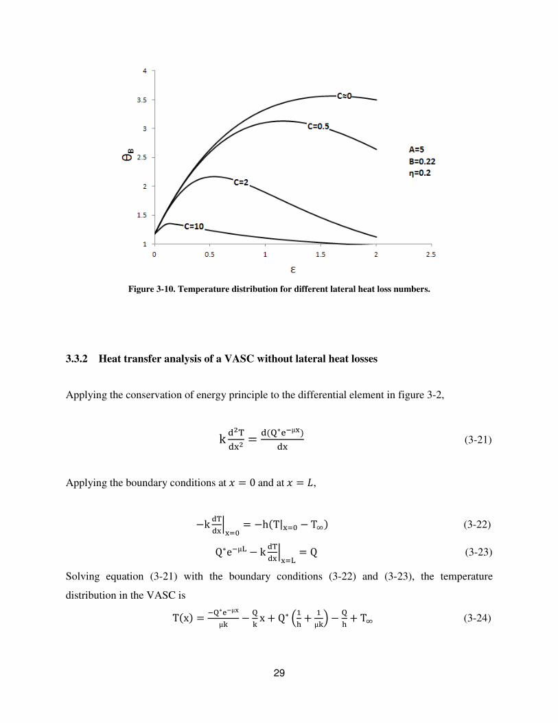
� The lateral heat loss number C (Eq. 3-12)
C � x 4h�kD�-
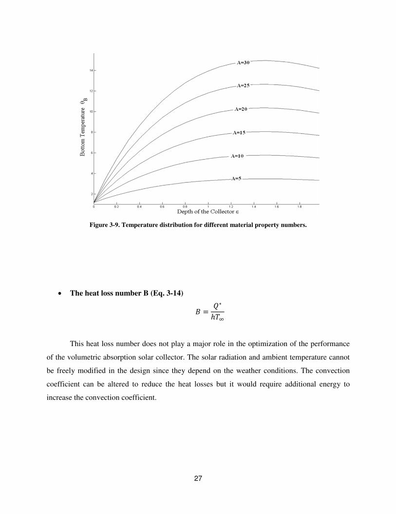
This work studied a cylindrical VASC with a diameter D. It was shown that the increase
in the value of C results in the increase of the lateral heat losses which negatively affect the
performance of the collector. Therefore, it is important to design a VASC that has the minimum
possible value of C. From the expression above (Eq. 3-12), it can be seen that the C value could
be minimized by increasing the values of k, µ and D or decreasing the value of hL. However,
choosing materials with high values of k and µ is not an option since this will lower the value of
A and negatively affect the performance. Therefore, only D, the diameter of the collector, and hL
can be manipulated. hL represents the convection coefficient between the collector and the
surrounding. The value of hL depends heavily on the quality and size of material chosen for
insulation as shown in equation 3-12. If the insulation material has a low thermal conductivity
and a large diameter, the h�value will be reduced. The advantage of a large diameter for a VASC
is two-fold: the larger the diameter is the more surface area and therefore more radiation is
collected; the second advantage is that for larger diameters, the values of C are increasingly
lower, which means that less heat is lost through the lateral surfaces of the collector. Figure 3-10
shows the variation of the collector’s bottom temperature with respect to the depth of the
collector for C y 0, C � 0.5, C � 2 and for C � 10. From the figure, it can be seen that lower
values of C lead to less heat losses and result in higher temperatures of the collector.
29
Figure 3-10. Temperature distribution for different lateral heat loss numbers.
3.3.2 Heat transfer analysis of a VASC without lateral heat losses
Applying the conservation of energy principle to the differential element in figure 3-2,
k $� �$ � �� z{µ�� � (3-21)
Applying the boundary conditions at | � 0 and at | � },
~ �k � ����e � �h�~T|��e � T̂ � (3-22) Q e"µ� � k ~ � ����� � Q (3-23)
Solving equation (3-21) with the boundary conditions (3-22) and (3-23), the temperature
distribution in the VASC is
T�x� � "� z{µ�µ& � �& x % Q 4;' % ;µ&7 � �' % T̂ (3-24)
30
which, in dimensionless form, can be written as
θ � A�1 � ηx� � e��� % B�1 � η� (3-25)
And the temperature at the bottom of the collector (| � }) is
θX � A�1 � ηε � eY� % B�1 � η� (3-26)
Equation 3-26 can be rearranged to find the efficiency of a VASC as a function of the material
property number, A, heat loss number, B, dimensionless depth number ε and the bottom
temperature of the collector ��
η � *"*z�AX*YAX � ;*YAX �θX � 1� � �� (3-27)
With careful selection of parameters, the dimensionless number C can be driven to almost
zero. When the C value is approximately equal to zero, the effects of lateral heat losses are
minimized or reduced to zero, resulting in the optimum performance of the collector: higher
temperatures can be reached at high efficiencies. The following analysis studies the performance
of the collector without lateral heat losses. The efficiency with respect to the temperature for
different depths of the collector is presented for three different cases. The first case assumes
normal operating conditions, with the sun providing radiation at 1000 W/m2 and at an ambient
temperature of 300 K, with a low quality glass material such as the one used in the experimental
analysis section. The second case tries to maintain the same operating conditions but uses a
better quality of glass for this application. A glass material is considered high quality if the
product of its coefficient of conduction, u, and its extinction coefficient, μ, is very small. The
third case seeks to improve the performance of the collector by using a good quality glass
material and reducing the convection heat losses by installing a glass cover on top of the
collector, which lowers the value of w. Below is a summary of the three cases in a table.
31
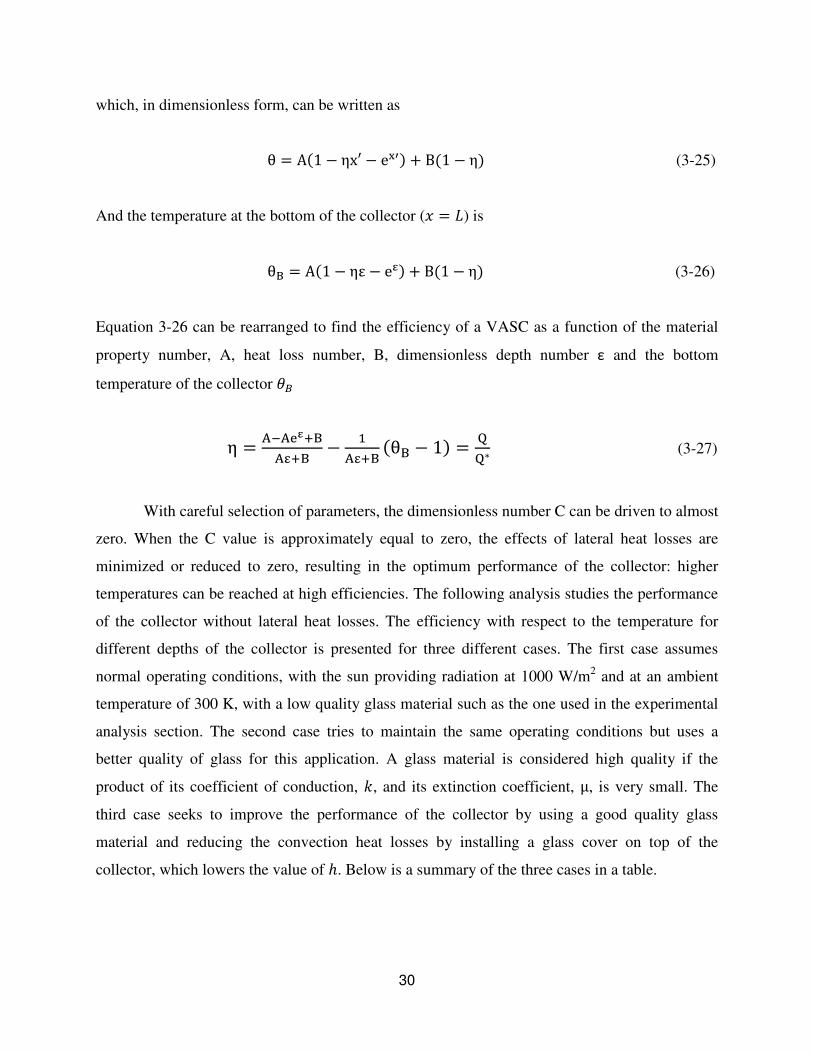
Table 3-1 Parameters for the analysis of the efficiency of the VASC.
Q* Tinf µk h
(W/m2) (K) (W/m2K) (W/m2K)
Case I 1000 300 5 20
Case II 1000 300 1.25 20
Case III 1000 300 1.25 5
Figure 3-11. Efficiency with respect to temperature - Case I.
From figure 3-11, if a VASC with a depth of 10 centimeters is considered, and under the
conditions stated in case 1, temperatures of around 100oC can be reached with an efficiency of
20%. It can also be noticed from the same figure that thinner VASCs reach higher efficiencies
for low temperature applications but the efficiency decreases fast with the increase of
temperature. VASC with a bigger depth have a lower but relatively steady efficiency and are
more practical for higher temperature applications.
0
0.2
0.4
0.6
0.8
1
0 50 100 150 200
η
T-Tinf
L = 0.01 m
L = 0.05 m
L = 0.1 m
L = 0.5 m
L = 0.3 m
32
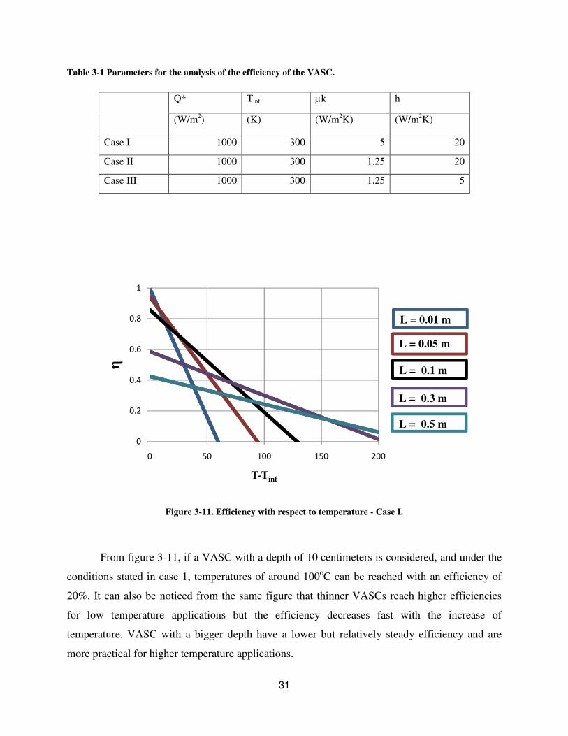
Figure 3-12. Efficiency with respect to temperature - Case II.
For case 2 (figure 3-12), the same VASC of 10 centimeters reaches the temperatures of
around 100oC with a much bigger efficiency of 60%. It’s very clear that minimizing the product
μu improves dramatically the performance of the collector. In this particular case, a 200%
increase in efficiency was achieved by reducing the value of μu to 25%. Like in the previous
case (case 1), it can be seen that the thicker the VASC is the steadier the efficiency and the better
the performance at high temperatures.
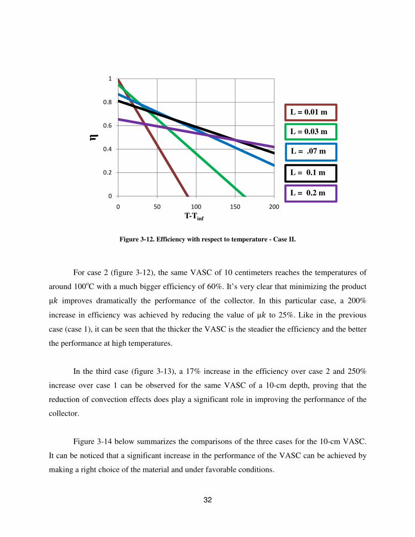
In the third case (figure 3-13), a 17% increase in the efficiency over case 2 and 250%
increase over case 1 can be observed for the same VASC of a 10-cm depth, proving that the
reduction of convection effects does play a significant role in improving the performance of the
collector.
Figure 3-14 below summarizes the comparisons of the three cases for the 10-cm VASC.
It can be noticed that a significant increase in the performance of the VASC can be achieved by
making a right choice of the material and under favorable conditions.
0
0.2
0.4
0.6
0.8
1
0 50 100 150 200
η
T-Tinf
L = 0.01 m
L = 0.03 m
L = .07 m
L = 0.1 m
L = 0.2 m
33
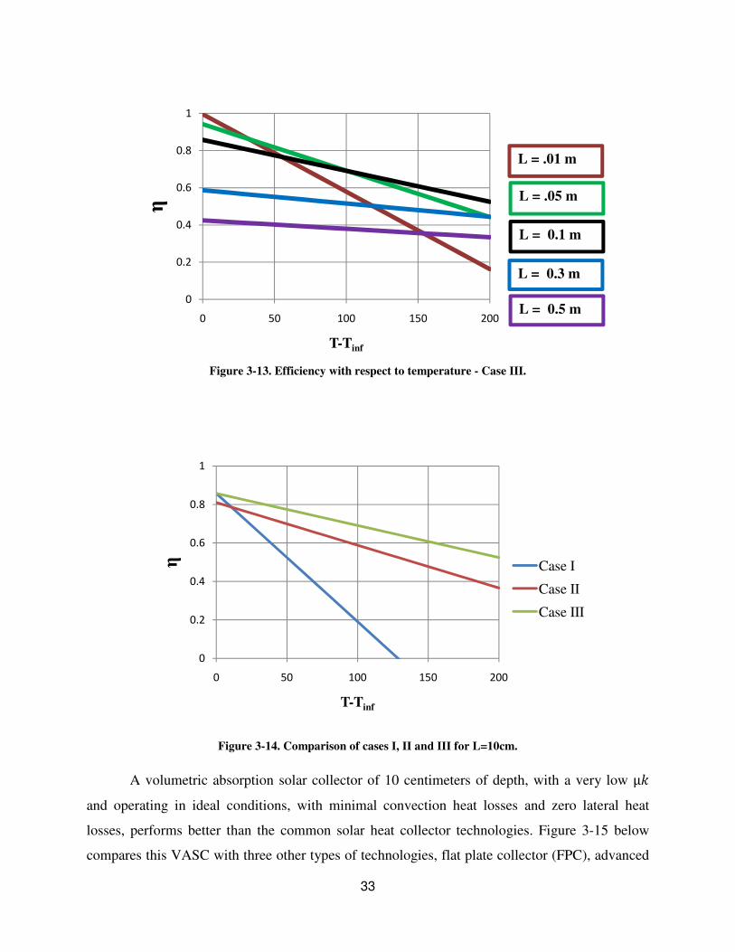
Figure 3-13. Efficiency with respect to temperature - Case III.
Figure 3-14. Comparison of cases I, II and III for L=10cm.
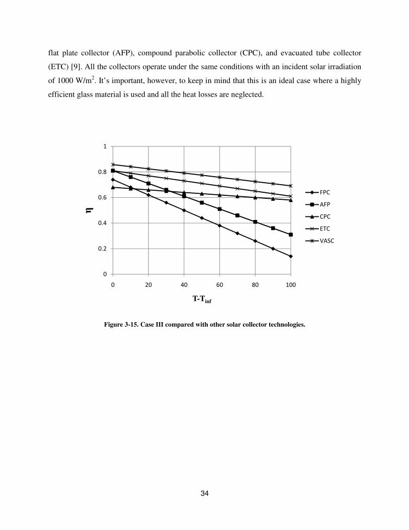
A volumetric absorption solar collector of 10 centimeters of depth, with a very low μu
and operating in ideal conditions, with minimal convection heat losses and zero lateral heat
losses, performs better than the common solar heat collector technologies. Figure 3-15 below
compares this VASC with three other types of technologies, flat plate collector (FPC), advanced
0
0.2
0.4
0.6
0.8
1
0 50 100 150 200
η
T-Tinf
L = .01 m
L = .05 m
L = 0.1 m
L = 0.3 m
L = 0.5 m
0
0.2
0.4
0.6
0.8
1
0 50 100 150 200
η
T-Tinf
Case I
Case II
Case III
34
flat plate collector (AFP), compound parabolic collector (CPC), and evacuated tube collector
(ETC) [9]. All the collectors operate under the same conditions with an incident solar irradiation
of 1000 W/m2. It’s important, however, to keep in mind that this is an ideal case where a highly
efficient glass material is used and all the heat losses are neglected.
Figure 3-15. Case III compared with other solar collector technologies.
0
0.2
0.4
0.6
0.8
1
0 20 40 60 80 100
η
T-Tinf
FPC
AFP
CPC
ETC
VASC
35
CHAPTER FOUR
4 THE VOLUMETRIC ABSORPTION SOLAR COLLECTOR:
EXPERIMENTAL ANALYSIS
4.1 Introduction
In order to validate the model discussed above, a series of laboratory experiments were
set up using a semitransparent material. The choice for the material was a one foot long
Borosilicate Glass rod with 1.2 inch diameter. This material was chosen due to its off-the-counter
availability in retail stores and relatively cheap cost. It also comes with the manufacturer’s
estimated thermodynamic properties such as the coefficient of thermal conductivity, the melting
point and the specific heat capacity. Experiments were carried out to determine two main
quantities: the extinction coefficient of the material and the temperature distribution. The top
surface of the rod was exposed to a light source in such a way that the radiation is normal to the
surface. Incident radiation was measured at the top surface of the rod and transmitted radiation
was measured at the bottom of the rod. To measure the temperature, six calibrated high precision
thermistors were uniformly attached to the cylinder to measure the temperature. A Labview
program was used to record temperature data from the thermistors. In this experimental setup,
precaution was taken to minimize the energy losses in the lateral surface of the cylinder and
fiberglass was used to achieve this insulation. The experimental results were found to be only
within a 2% difference with the theoretical prediction.
4.2 Determination of the extinction coefficient
The surface of the borosilicate cylinder was exposed to a light source. It is important to
note that this radiation hitting the surface has spectral as well as directional distribution
determined by ���, �, ��. This quantity is defined as the rate at which radiant energy of
wavelength � is incident from the (�, � ) direction, per unit area of the intercepting surface
36
normal to this direction, per unit solid angle about this direction, and per unit wavelength interval
�� about � [21].
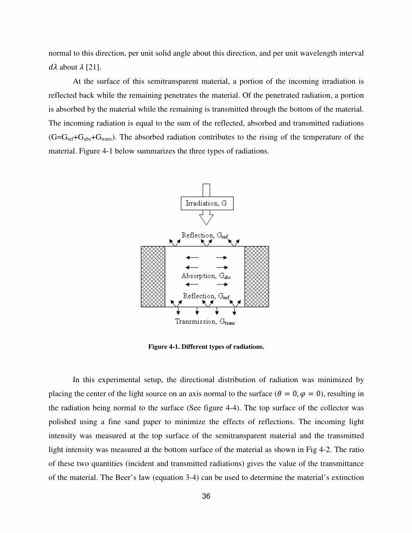
At the surface of this semitransparent material, a portion of the incoming irradiation is
reflected back while the remaining penetrates the material. Of the penetrated radiation, a portion
is absorbed by the material while the remaining is transmitted through the bottom of the material.
The incoming radiation is equal to the sum of the reflected, absorbed and transmitted radiations
(G=Gref+Gabs+Gtrans). The absorbed radiation contributes to the rising of the temperature of the
material. Figure 4-1 below summarizes the three types of radiations.
Figure 4-1. Different types of radiations.
In this experimental setup, the directional distribution of radiation was minimized by
placing the center of the light source on an axis normal to the surface (� � 0, � � 0), resulting in
the radiation being normal to the surface (See figure 4-4). The top surface of the collector was
polished using a fine sand paper to minimize the effects of reflections. The incoming light
intensity was measured at the top surface of the semitransparent material and the transmitted
light intensity was measured at the bottom surface of the material as shown in Fig 4-2. The ratio
of these two quantities (incident and transmitted radiations) gives the value of the transmittance
of the material. The Beer’s law (equation 3-4) can be used to determine the material’s extinction
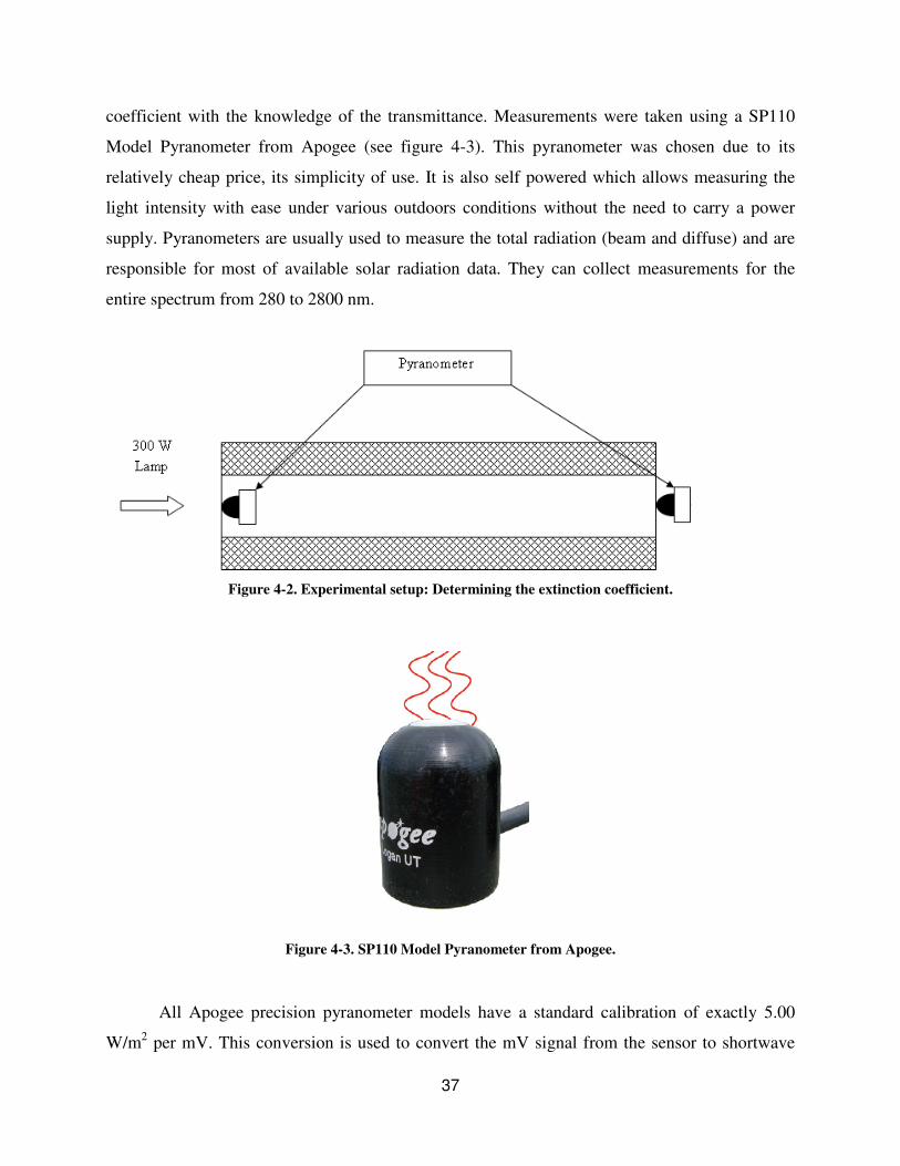
37
coefficient with the knowledge of the transmittance. Measurements were taken using a SP110
Model Pyranometer from Apogee (see figure 4-3). This pyranometer was chosen due to its
relatively cheap price, its simplicity of use. It is also self powered which allows measuring the
light intensity with ease under various outdoors conditions without the need to carry a power
supply. Pyranometers are usually used to measure the total radiation (beam and diffuse) and are
responsible for most of available solar radiation data. They can collect measurements for the
entire spectrum from 280 to 2800 nm.
Figure 4-2. Experimental setup: Determining the extinction coefficient.
Figure 4-3. SP110 Model Pyranometer from Apogee.
All Apogee precision pyranometer models have a standard calibration of exactly 5.00
W/m2 per mV. This conversion is used to convert the mV signal from the sensor to shortwave
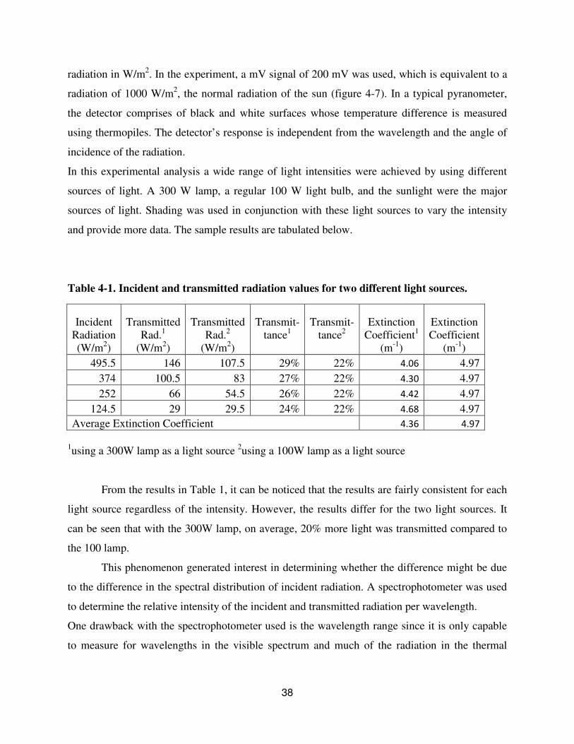
38
radiation in W/m2. In the experiment, a mV signal of 200 mV was used, which is equivalent to a
radiation of 1000 W/m2, the normal radiation of the sun (figure 4-7). In a typical pyranometer,
the detector comprises of black and white surfaces whose temperature difference is measured
using thermopiles. The detector’s response is independent from the wavelength and the angle of
incidence of the radiation.
In this experimental analysis a wide range of light intensities were achieved by using different
sources of light. A 300 W lamp, a regular 100 W light bulb, and the sunlight were the major
sources of light. Shading was used in conjunction with these light sources to vary the intensity
and provide more data. The sample results are tabulated below.
Table 4-1. Incident and transmitted radiation values for two different light sources.
Incident Radiation (W/m2)
Transmitted Rad.1
(W/m2)
Transmitted Rad.2
(W/m2)
Transmit-tance1
Transmit-tance2
Extinction Coefficient1
(m-1)
Extinction Coefficient
(m-1)
495.5 146 107.5 29% 22% 4.06 4.97
374 100.5 83 27% 22% 4.30 4.97
252 66 54.5 26% 22% 4.42 4.97
124.5 29 29.5 24% 22% 4.68 4.97
Average Extinction Coefficient 4.36 4.97
1using a 300W lamp as a light source 2using a 100W lamp as a light source
From the results in Table 1, it can be noticed that the results are fairly consistent for each
light source regardless of the intensity. However, the results differ for the two light sources. It
can be seen that with the 300W lamp, on average, 20% more light was transmitted compared to
the 100 lamp.
This phenomenon generated interest in determining whether the difference might be due
to the difference in the spectral distribution of incident radiation. A spectrophotometer was used
to determine the relative intensity of the incident and transmitted radiation per wavelength.
One drawback with the spectrophotometer used is the wavelength range since it is only capable
to measure for wavelengths in the visible spectrum and much of the radiation in the thermal
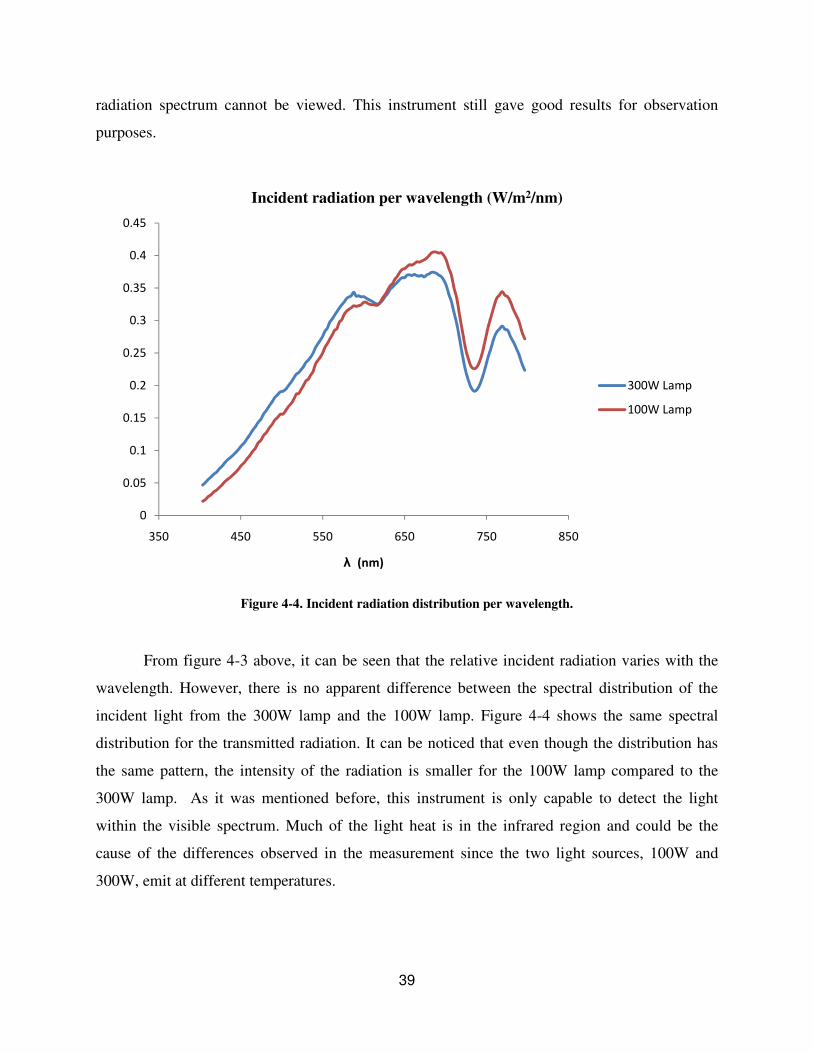
39
radiation spectrum cannot be viewed. This instrument still gave good results for observation
purposes.
Figure 4-4. Incident radiation distribution per wavelength.
From figure 4-3 above, it can be seen that the relative incident radiation varies with the
wavelength. However, there is no apparent difference between the spectral distribution of the
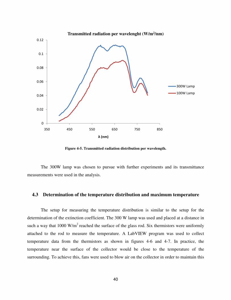
incident light from the 300W lamp and the 100W lamp. Figure 4-4 shows the same spectral
distribution for the transmitted radiation. It can be noticed that even though the distribution has
the same pattern, the intensity of the radiation is smaller for the 100W lamp compared to the
300W lamp. As it was mentioned before, this instrument is only capable to detect the light
within the visible spectrum. Much of the light heat is in the infrared region and could be the
cause of the differences observed in the measurement since the two light sources, 100W and
300W, emit at different temperatures.
0
0.05
0.1
0.15
0.2
0.25
0.3
0.35
0.4
0.45
350 450 550 650 750 850
λ (nm)
Incident radiation per wavelength (W/m2/nm)
300W Lamp
100W Lamp
40
Figure 4-5. Transmitted radiation distribution per wavelength.
The 300W lamp was chosen to pursue with further experiments and its transmittance
measurements were used in the analysis.
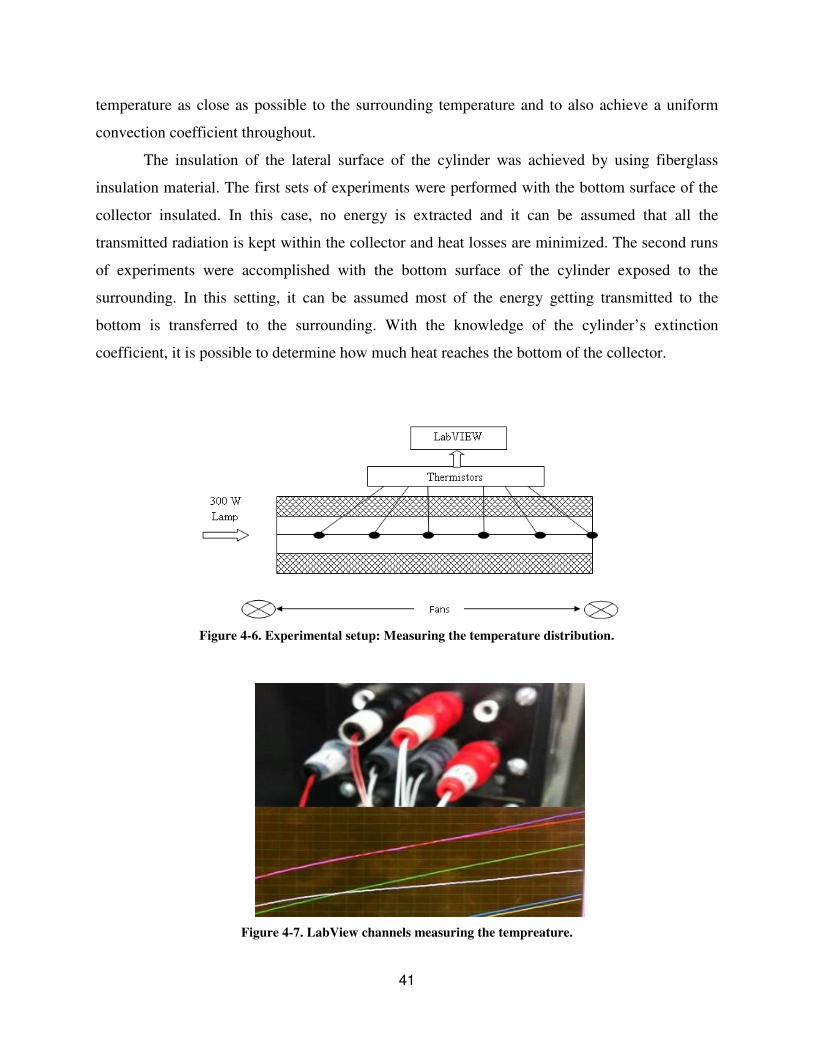
4.3 Determination of the temperature distribution and maximum temperature
The setup for measuring the temperature distribution is similar to the setup for the
determination of the extinction coefficient. The 300 W lamp was used and placed at a distance in
such a way that 1000 W/m2 reached the surface of the glass rod. Six thermistors were uniformly
attached to the rod to measure the temperature. A LabVIEW program was used to collect
temperature data from the thermistors as shown in figures 4-6 and 4-7. In practice, the
temperature near the surface of the collector would be close to the temperature of the
surrounding. To achieve this, fans were used to blow air on the collector in order to maintain this
0
0.02
0.04
0.06
0.08
0.1
0.12
350 450 550 650 750 850
λ (nm)
Transmitted radiation per wavelenght (W/m2/nm)
300W Lamp
100W Lamp
41
temperature as close as possible to the surrounding temperature and to also achieve a uniform
convection coefficient throughout.
The insulation of the lateral surface of the cylinder was achieved by using fiberglass
insulation material. The first sets of experiments were performed with the bottom surface of the
collector insulated. In this case, no energy is extracted and it can be assumed that all the
transmitted radiation is kept within the collector and heat losses are minimized. The second runs
of experiments were accomplished with the bottom surface of the cylinder exposed to the
surrounding. In this setting, it can be assumed most of the energy getting transmitted to the
bottom is transferred to the surrounding. With the knowledge of the cylinder’s extinction
coefficient, it is possible to determine how much heat reaches the bottom of the collector.
Figure 4-6. Experimental setup: Measuring the temperature distribution.
Figure 4-7. LabView channels measuring the tempreature.
42
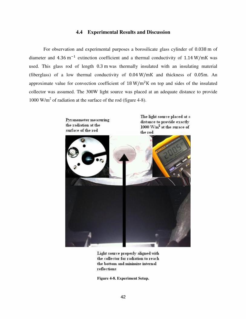
4.4 Experimental Results and Discussion
For observation and experimental purposes a borosilicate glass cylinder of 0.038 m of
diameter and 4.36 m"; extinction coefficient and a thermal conductivity of 1.14 W/mK was
used. This glass rod of length 0.3 m was thermally insulated with an insulating material
(fiberglass) of a low thermal conductivity of 0.04 W/mK and thickness of 0.05m. An
approximate value for convection coefficient of 18 W/m-K on top and sides of the insulated
collector was assumed. The 300W light source was placed at an adequate distance to provide
1000 W/m2 of radiation at the surface of the rod (figure 4-8).
Figure 4-8. Experiment Setup.
43
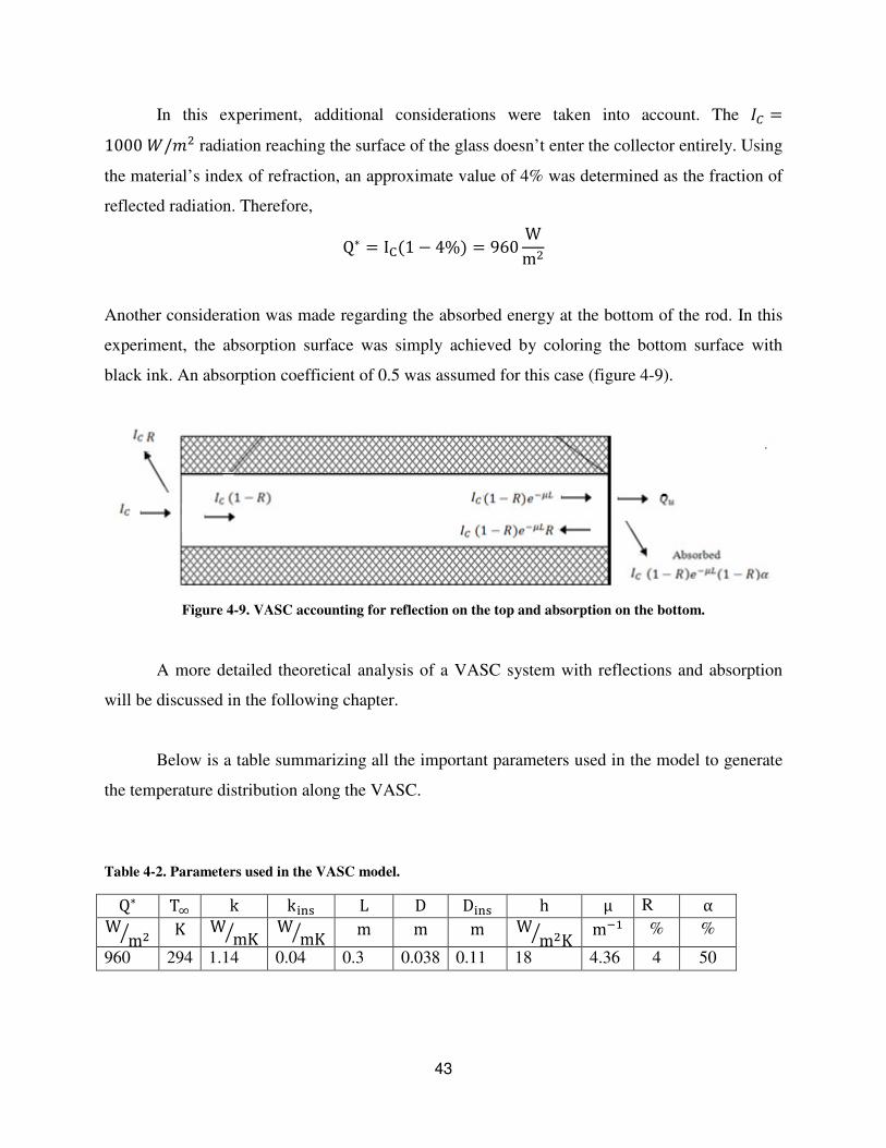
In this experiment, additional considerations were taken into account. The �� �1000 �/�- radiation reaching the surface of the glass doesn’t enter the collector entirely. Using
the material’s index of refraction, an approximate value of 4% was determined as the fraction of
reflected radiation. Therefore,
Q � IJ�1 � 4%� � 960 Wm-
Another consideration was made regarding the absorbed energy at the bottom of the rod. In this
experiment, the absorption surface was simply achieved by coloring the bottom surface with
black ink. An absorption coefficient of 0.5 was assumed for this case (figure 4-9).
Figure 4-9. VASC accounting for reflection on the top and absorption on the bottom.
A more detailed theoretical analysis of a VASC system with reflections and absorption
will be discussed in the following chapter.
Below is a table summarizing all the important parameters used in the model to generate
the temperature distribution along the VASC.
Table 4-2. Parameters used in the VASC model.
Q T̂ k kC�� L D DC�� h µ R α W m-q K W mKq W mKq m m m W m-Kq m"; % %
960 294 1.14 0.04 0.3 0.038 0.11 18 4.36 4 50
44
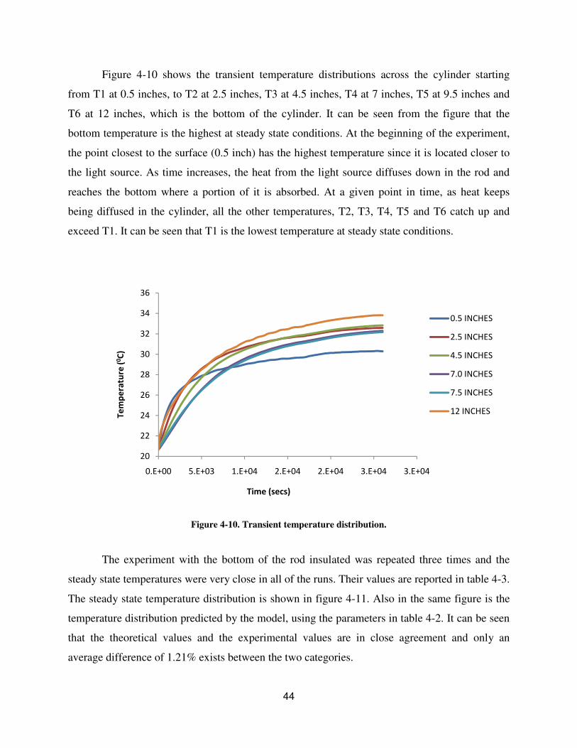
Figure 4-10 shows the transient temperature distributions across the cylinder starting
from T1 at 0.5 inches, to T2 at 2.5 inches, T3 at 4.5 inches, T4 at 7 inches, T5 at 9.5 inches and
T6 at 12 inches, which is the bottom of the cylinder. It can be seen from the figure that the
bottom temperature is the highest at steady state conditions. At the beginning of the experiment,
the point closest to the surface (0.5 inch) has the highest temperature since it is located closer to
the light source. As time increases, the heat from the light source diffuses down in the rod and
reaches the bottom where a portion of it is absorbed. At a given point in time, as heat keeps
being diffused in the cylinder, all the other temperatures, T2, T3, T4, T5 and T6 catch up and
exceed T1. It can be seen that T1 is the lowest temperature at steady state conditions.
Figure 4-10. Transient temperature distribution.
The experiment with the bottom of the rod insulated was repeated three times and the
steady state temperatures were very close in all of the runs. Their values are reported in table 4-3.
The steady state temperature distribution is shown in figure 4-11. Also in the same figure is the
temperature distribution predicted by the model, using the parameters in table 4-2. It can be seen
that the theoretical values and the experimental values are in close agreement and only an
average difference of 1.21% exists between the two categories.
20
22
24
26
28
30
32
34
36
0.E+00 5.E+03 1.E+04 2.E+04 2.E+04 3.E+04 3.E+04
Te
mp
era
ture
(0C
)
Time (secs)
0.5 INCHES
2.5 INCHES
4.5 INCHES
7.0 INCHES
7.5 INCHES
12 INCHES
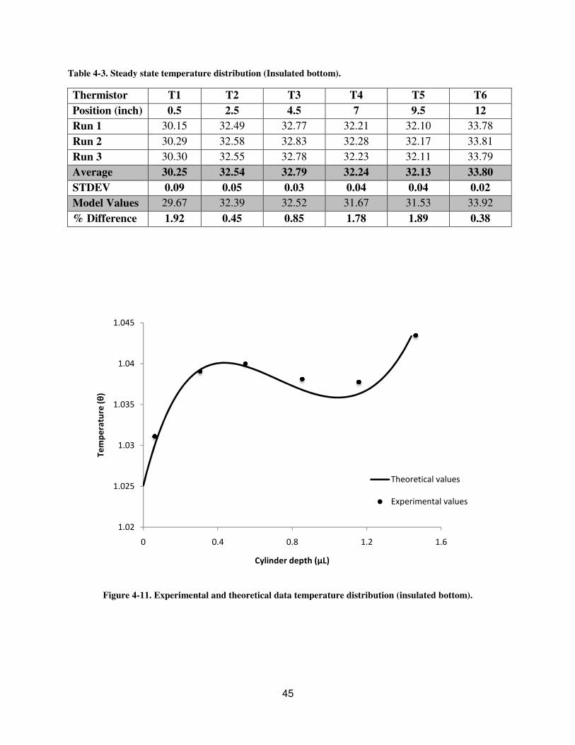
Table 4-3. Steady state temperature d
Thermistor T1
Position (inch) 0.5
Run 1 30.15
Run 2 30.29
Run 3 30.30
Average 30.25
STDEV 0.09
Model Values 29.67
% Difference 1.92
Figure 4-11. Experimental an
1.02
1.025
1.03
1.035
1.04
1.045
0 0.4
Te
mp
era
ture
(θ
)
45
e distribution (Insulated bottom).
T2 T3 T4 T5
2.5 4.5 7 9.5
32.49 32.77 32.21 32.10
32.58 32.83 32.28 32.17
32.55 32.78 32.23 32.11
32.54 32.79 32.24 32.13
0.05 0.03 0.04 0.04
32.39 32.52 31.67 31.53
0.45 0.85 1.78 1.89
l and theoretical data temperature distribution (insulated
0.4 0.8 1.2
Cylinder depth (μL)
Theoretical
Experiment
T6
12
10 33.78
17 33.81
11 33.79
13 33.80
0.02
53 33.92
0.38
ted bottom).
1.6
ical values
ental values
46
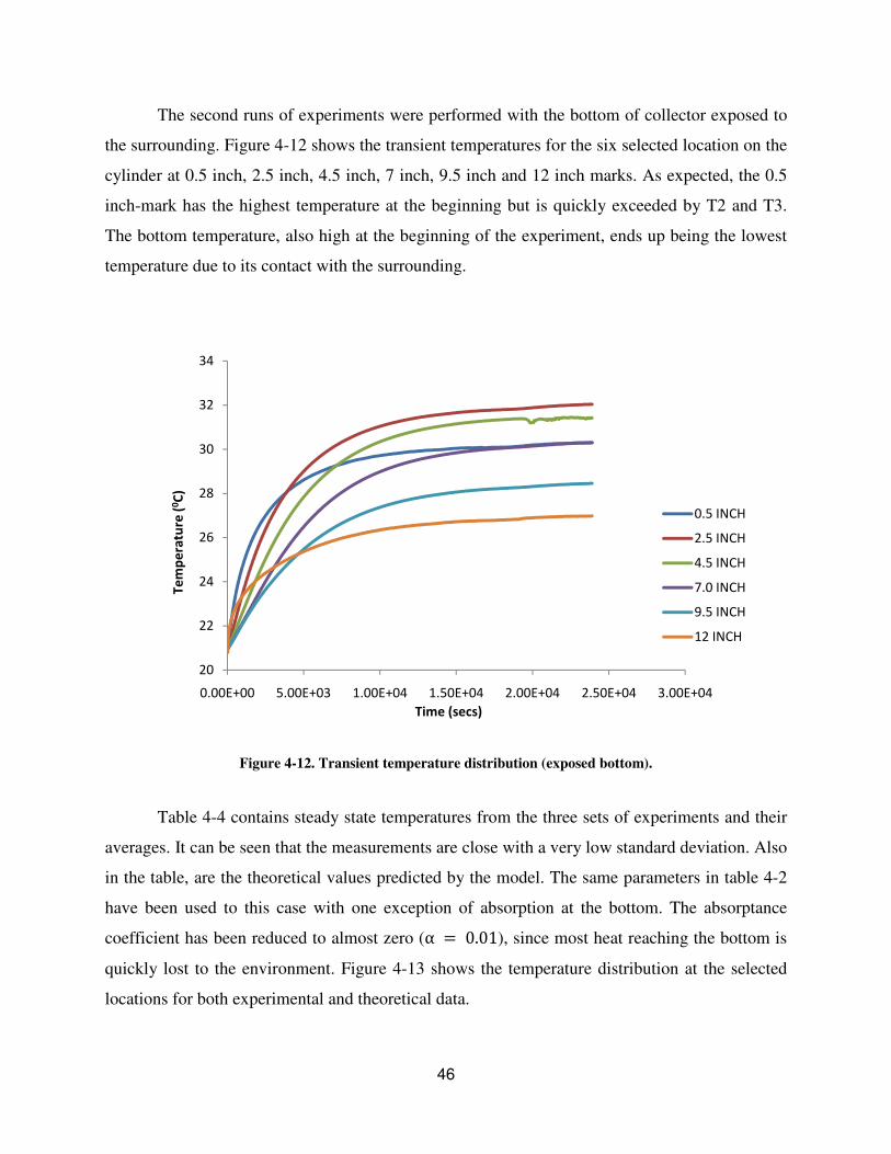
The second runs of experiments were performed with the bottom of collector exposed to
the surrounding. Figure 4-12 shows the transient temperatures for the six selected location on the
cylinder at 0.5 inch, 2.5 inch, 4.5 inch, 7 inch, 9.5 inch and 12 inch marks. As expected, the 0.5
inch-mark has the highest temperature at the beginning but is quickly exceeded by T2 and T3.
The bottom temperature, also high at the beginning of the experiment, ends up being the lowest
temperature due to its contact with the surrounding.
Figure 4-12. Transient temperature distribution (exposed bottom).
Table 4-4 contains steady state temperatures from the three sets of experiments and their
averages. It can be seen that the measurements are close with a very low standard deviation. Also
in the table, are the theoretical values predicted by the model. The same parameters in table 4-2
have been used to this case with one exception of absorption at the bottom. The absorptance
coefficient has been reduced to almost zero (α � 0.01), since most heat reaching the bottom is
quickly lost to the environment. Figure 4-13 shows the temperature distribution at the selected
locations for both experimental and theoretical data.
20
22
24
26
28
30
32
34
0.00E+00 5.00E+03 1.00E+04 1.50E+04 2.00E+04 2.50E+04 3.00E+04
Te
mp
era
ture
(0C
)
Time (secs)
0.5 INCH
2.5 INCH
4.5 INCH
7.0 INCH
9.5 INCH
12 INCH
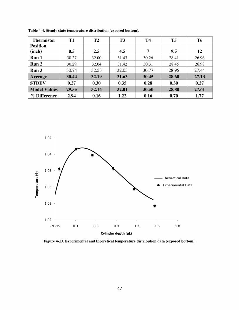
Table 4-4. Steady state temperature d
Thermistor T1
Position
(inch) 0.5
Run 1 30.27
Run 2 30.29
Run 3 30.74
Average 30.44
STDEV 0.27
Model Values 29.55
% Difference 2.94
Figure 4-13. Experimental a
1.02
1.02
1.03
1.03
1.04
1.04
-2E-15 0.3
Te
mp
era
ture
(θ
)
47
e distribution (exposed bottom).
T2 T3 T4 T5
2.5 4.5 7 9.5
32.00 31.43 30.26 28.41
32.04 31.42 30.31 28.45
32.53 32.03 30.77 28.95
32.19 31.63 30.45 28.60
0.30 0.35 0.28 0.30
32.14 32.01 30.50 28.80
0.16 1.22 0.16 0.70
l and theoretical temperature distribution data (exposed
0.6 0.9 1.2 1.5 1.8
Cylinder depth (μL)
Theoretical
Experiment
T6
12
26.96
26.98
95 27.44
60 27.13
0.27
80 27.61
1.77
ed bottom).
1.8
tical Data
ental Data
48
CHAPTER FIVE
5 LOCATING POTENTIAL APPLICATIONS OF THE
VOLUMETRIC ABSORPTION SOLAR COLLECTOR
5.1 Introduction
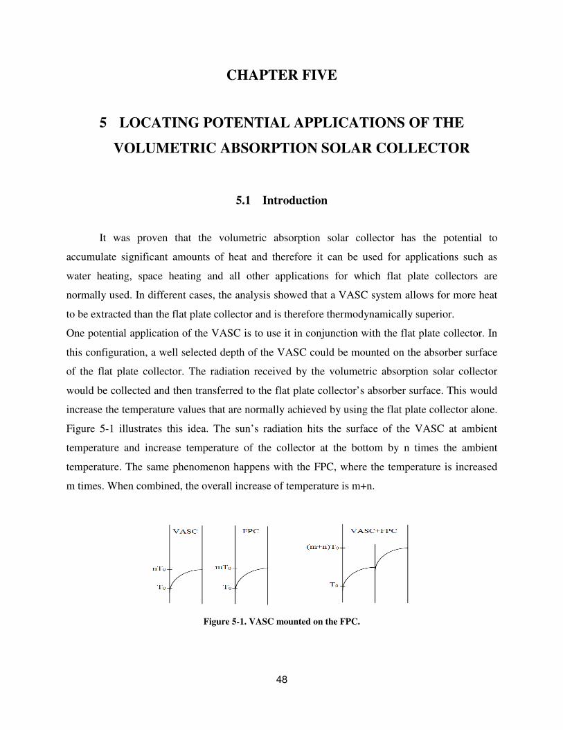
It was proven that the volumetric absorption solar collector has the potential to
accumulate significant amounts of heat and therefore it can be used for applications such as
water heating, space heating and all other applications for which flat plate collectors are
normally used. In different cases, the analysis showed that a VASC system allows for more heat
to be extracted than the flat plate collector and is therefore thermodynamically superior.
One potential application of the VASC is to use it in conjunction with the flat plate collector. In
this configuration, a well selected depth of the VASC could be mounted on the absorber surface
of the flat plate collector. The radiation received by the volumetric absorption solar collector
would be collected and then transferred to the flat plate collector’s absorber surface. This would
increase the temperature values that are normally achieved by using the flat plate collector alone.
Figure 5-1 illustrates this idea. The sun’s radiation hits the surface of the VASC at ambient
temperature and increase temperature of the collector at the bottom by n times the ambient
temperature. The same phenomenon happens with the FPC, where the temperature is increased
m times. When combined, the overall increase of temperature is m+n.
Figure 5-1. VASC mounted on the FPC.
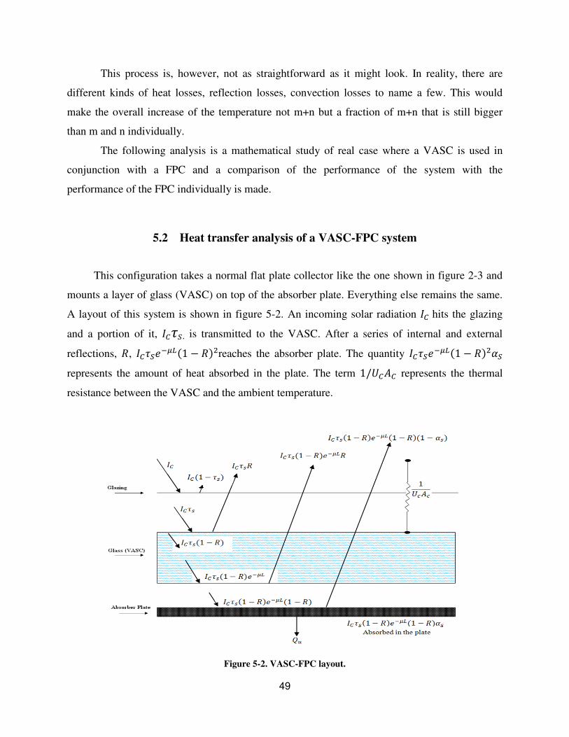
49
This process is, however, not as straightforward as it might look. In reality, there are
different kinds of heat losses, reflection losses, convection losses to name a few. This would
make the overall increase of the temperature not m+n but a fraction of m+n that is still bigger
than m and n individually.
The following analysis is a mathematical study of real case where a VASC is used in
conjunction with a FPC and a comparison of the performance of the system with the
performance of the FPC individually is made.
5.2 Heat transfer analysis of a VASC-FPC system
This configuration takes a normal flat plate collector like the one shown in figure 2-3 and
mounts a layer of glass (VASC) on top of the absorber plate. Everything else remains the same.
A layout of this system is shown in figure 5-2. An incoming solar radiation �� hits the glazing
and a portion of it, ���� , is transmitted to the VASC. After a series of internal and external
reflections, �, �����"���1 � ��-reaches the absorber plate. The quantity �����"���1 � ��-��
represents the amount of heat absorbed in the plate. The term 1/��r� represents the thermal
resistance between the VASC and the ambient temperature.
Figure 5-2. VASC-FPC layout.
50
Applying the conservation of energy principle to the VASC, we get
k $� �$ � ��� ��;"¡�z{µ�� � (5-1)
where Ic is the incident radiation hitting the glazing surface, τs is the reflection coefficient and R
is the reflected radiation. This is similar to equation 3-21, with Q* = Ic τs(1-R)
Applying the boundary conditions at | � 0 and at | � },
~ �k � ����e � �U�~T|��e � T̂ � (5-2)
IJτ��1 � R�e"µ��1 � R�α� � k ~ � ����� � Q¤ (5-3)
where Uc is the equivalent convection coefficient between the glass material and the ambient,
and αs is the absorptance of the glass. These boundary conditions are similar to the ones found in
equations 3-22 and 3-23.
The equation can be solved to arrive at the final form of the heat conducted in the absorber plate,
which is
Q � Q¤ % Q e"µ��1 � α��1 � R�� (5-4)
where Q is the total heat reaching the bottom of the glass, Q* is the radiation entering the glass
material, and Qu is the heat extracted and ready to be used.
5.2.1 The efficiency of the system
For the VASC component of the system,
η � �� � �¥A� z{µ(O;"¦��;"¡�R� (5-5)
51
The overall efficiency of the system VASC-FPC is the ratio between the energy extracted from
the absorber plate Qu and the incident radiation that hits the top surface Ic
η���"§¨ � �¥�� � �¥� τ��1 � R� (5-6)
Combining equations 5-5 and 5-6 with equation 3-27, the overall efficiency of a combined
VASC-FPC as a function of the temperature difference can be found to be
η���"§¨ � τ��1 � R� ©*"*z�AX*YAX � e"YO1 � α��1 � R�Rª � ��;"¡��*YAX��« �TB � T∞� (5-7)
The equation 5-7 is a straight line in the k � d plane.
If the effects of reflections are disregarded and the ε value is set to ε=0, the above equation is
reduced to
秨 � τ�α� � ®��� �TB � T∞� (5-8)
which is the normal equation for the efficiency as a function of the temperature difference
between the plate and the ambient for a common flat plate collector [22].
The efficiency can also be expressed in terms of fixed losses (FL) and variable losses (VL) as
follows:
η � 1 � F� � V� (5-9)
For a common flat plate collector
F� � 1 � τ�α� (5-9a)
±²� V� � ®��� �TX � T̂ � (5-9b)
52
And for the VASC-FPC system
F� � 1 � τ��1 � R� ©*"*z�AX*YAX � e"YO1 � α��1 � R�Rª (5-9c)
±²� V� � ��;"¡��*YAX��« �TX � T̂ � (5-9d)
Finally, the efficiency can be expressed in terms of the temperature difference between the fluid
entering the collector and the ambient temperature, as it is usually done for the flat plate
collectors. The FL and VL values become:
For a common flat plate collector, the fixed losses and variable losses become
F� � 1 � F¡τ�α� (5-9e)
±²� V� � ³´®��� OT§,C� � T̂ R (5-9f)
And for the VASC-FPC system
F� � 1 � F¡τ��1 � R� ©*"*z�AX*YAX � e"YO1 � α��1 � R�Rª (5-9g)
±²� V� � ³´ ��;"¡��*YAX��« OT§,C� � T̂ R (5-9h)
where Tf,in is the temperature of the fluid entering the plate and FR is the heat removal factor.
The equation resulting from 5-9, 5-9e and 5-9f
η � 1 � �1 � F¡τ�α�� � ³´®��� OT§,C� � T̂ R (5-9i)
is known as the Hottel-Whillier-Bliss equation [22], which is the equation for the efficiency of a
flat plate collector in terms of fixed losses and variable losses and temperature difference
between the fluid and ambient.
53
5.2.2 Comparison between a FPC and a VASC-FPC
The comparison between the performances of the two systems can be based on their
efficiencies. But these efficiencies depend on the fixed losses and variable losses. Comparing
fixed losses and variable losses can give an idea of how the two systems perform.
Comparing fixed losses
From equations 5-9e and 5-9g, αs,eq can be defined as the equivalent absorptance of the VASC-
FPC system, therefore
α�,zµ � �1 � R� ©*"*z�AX*YAX � e"YO1 � α��1 � R�Rª (5-10)
Making substitution and rearranging the equation above, the equivalent absorptance can also be
written as
α�,zµ � α��1 � R�e"µ� % ;"¡4µ(µ¶A ·̧�7 ©4 ;µ& % ;®�7 �1 � e"µ�� � �& e"µ�ª (5-11)
And the ratio, ¹, between the equivalent absorptance of the VASC-FPC system, αs,eq, and the
absorptance of the common FPC, αs, can be determined
γ � ¦�,»¼¦� � �1 � R�e"µ� % ;"¡¦�4µ(µ¶A ·̧�7 U4 ;µ& % ;®�7 �1 � e"µ�� � �& e"µ�V (5-12)
If γ is greater than 1, then more energy is absorbed by the VASC-FPC system’s absorber plate
than the FPC alone, which increases the amount of heat delivered to the end user, Qu.
If this is the case, the VASC-FPC system has a better performance compared to the FPC in terms
of the fixed losses. If ¹ is less than 1, the VASC-FPC performance is poorer compared to FPC
alone in terms of the fixed losses.
54
Comparing variable losses
From equations 5-9h and 5-9f, Uc,eq can be defined as the equivalent Uc for the VASC-FPC
system, therefore
³´®�,»¼�½ � ³´ ��;"¡��*YAX��« (5-13)
Rearranging the equation above and making substitutions, the equivalent thermal resistance of
the overall VASC-FPC system is
;®�,»¼ � �& % ;®� (5-14)
The ratio, ρ, between the equivalent resistance of the combined system and the flat plate
collector alone is
;®�,»¼ ;®�¾ � ρ � 1 % µ�µ& U (5-15)
If ρ is greater than 1, the VASC-FPC thermal resistance is higher, which reduces the amount of
variable heat losses of the system and increases the overall performance. And if ρ is less than 1,
the VASC-FPC system is poorer than FPC in terms of variable losses.
The figures 5-3 and 5-4 show the variation of the ratios γ (figure 5-3) and ρ (figure 5-4)
with respect to the depth of the collector, for different types of glasses (µk) and for fixed
�� � 7.5 �/�-Á , � � 4% , and �� � 95%
It can be seen from figure 5-3 that the ratio γ is always less than 1 for the all the given glass
materials. This means that the fixed losses are larger for the VASC-FPC system compared to the
FPC alone. This puts the combined VASC-FPC system at a competitive disadvantage in
comparison to the common flat plate collector.
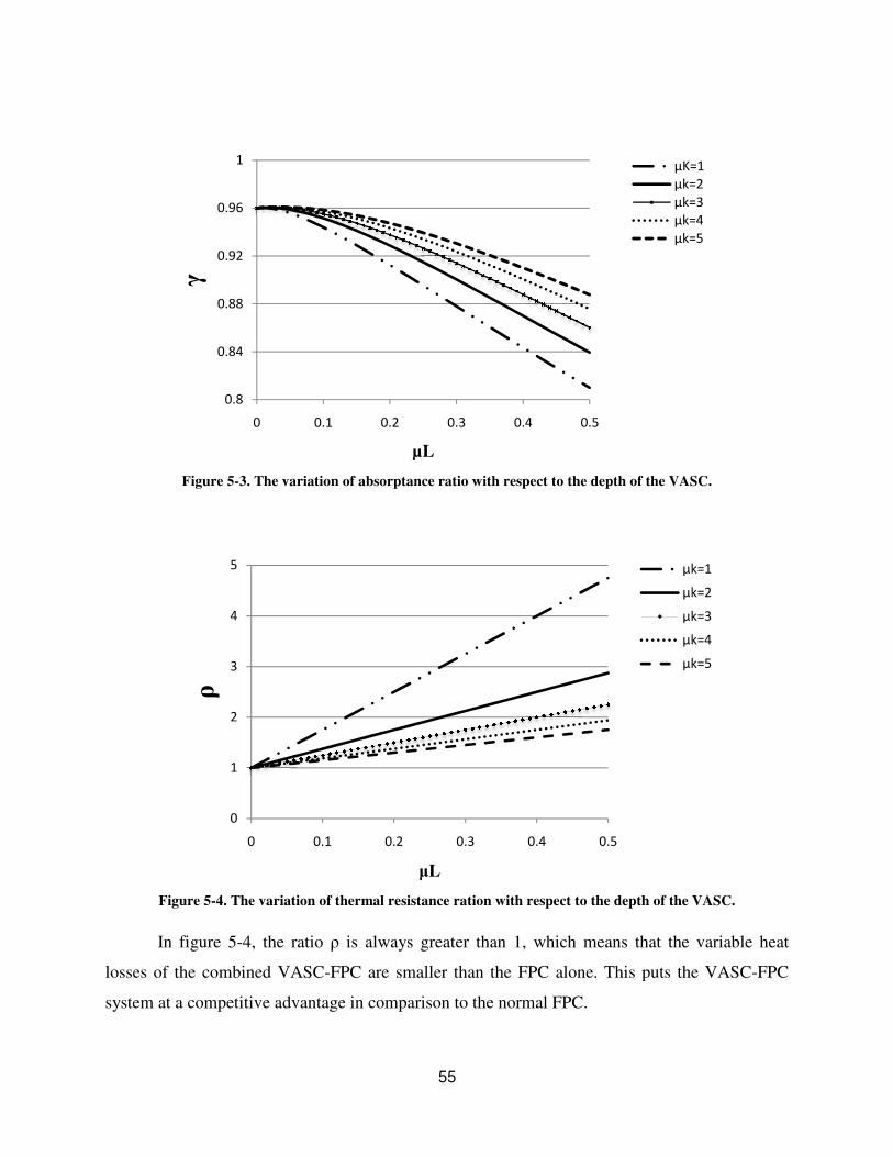
Figure 5-3. The variation
Figure 5-4. The variation of t
In figure 5-4, the ratio ρ
losses of the combined VASC-F
system at a competitive advantag
0.8
0.84
0.88
0.92
0.96
1
0 0.1
γ
0
1
2
3
4
5
0 0.1
ρ
55
on of absorptance ratio with respect to the depth of the V
f thermal resistance ration with respect to the depth of t
ρ is always greater than 1, which means that t
FPC are smaller than the FPC alone. This puts
tage in comparison to the normal FPC.
0.2 0.3 0.4 0.5
µL
0.2 0.3 0.4 0.5
�L
e VASC.
f the VASC.
t the variable heat
ts the VASC-FPC
µK=1
µk=2
µk=3
µk=4
µk=5
μk=1
μk=2
μk=3
μk=4
μk=5
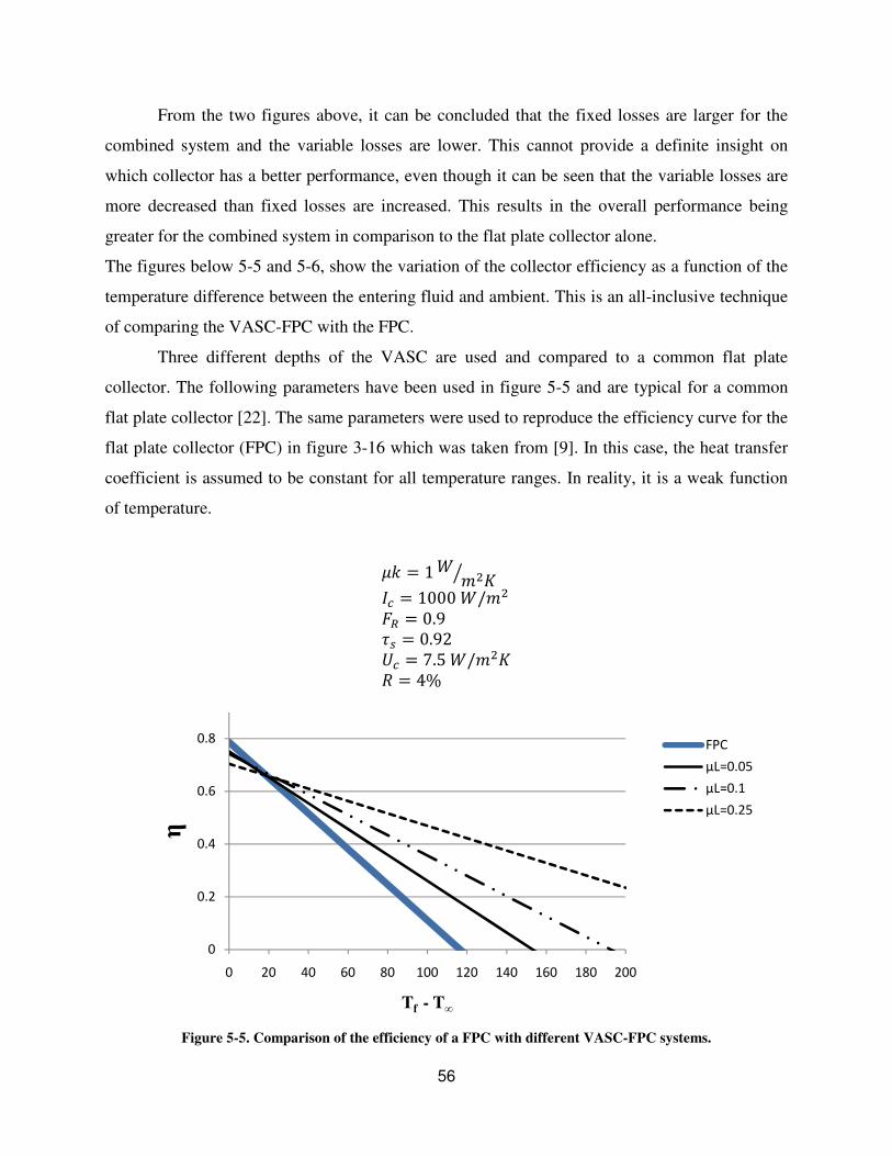
56
From the two figures above, it can be concluded that the fixed losses are larger for the
combined system and the variable losses are lower. This cannot provide a definite insight on
which collector has a better performance, even though it can be seen that the variable losses are
more decreased than fixed losses are increased. This results in the overall performance being
greater for the combined system in comparison to the flat plate collector alone.
The figures below 5-5 and 5-6, show the variation of the collector efficiency as a function of the
temperature difference between the entering fluid and ambient. This is an all-inclusive technique
of comparing the VASC-FPC with the FPC.
Three different depths of the VASC are used and compared to a common flat plate
collector. The following parameters have been used in figure 5-5 and are typical for a common
flat plate collector [22]. The same parameters were used to reproduce the efficiency curve for the
flat plate collector (FPC) in figure 3-16 which was taken from [9]. In this case, the heat transfer
coefficient is assumed to be constant for all temperature ranges. In reality, it is a weak function
of temperature.
tu � 1 � �-Áq � � 1000 �/�- ÃÄ � 0.9 �Å � 0.92 � � 7.5 �/�-Á � � 4%
Figure 5-5. Comparison of the efficiency of a FPC with different VASC-FPC systems.
0
0.2
0.4
0.6
0.8
0 20 40 60 80 100 120 140 160 180 200
η
Tf - T∞
FPC
μL=0.05
μL=0.1
μL=0.25
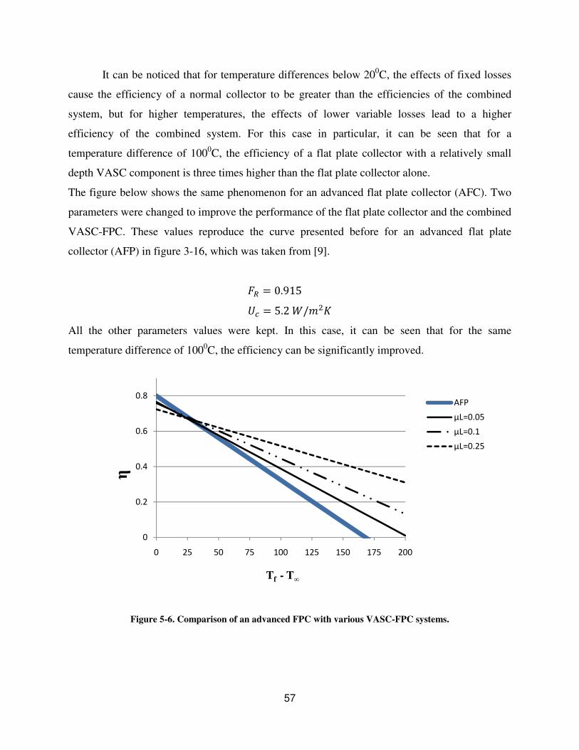
57
It can be noticed that for temperature differences below 200C, the effects of fixed losses
cause the efficiency of a normal collector to be greater than the efficiencies of the combined
system, but for higher temperatures, the effects of lower variable losses lead to a higher
efficiency of the combined system. For this case in particular, it can be seen that for a
temperature difference of 1000C, the efficiency of a flat plate collector with a relatively small
depth VASC component is three times higher than the flat plate collector alone.
The figure below shows the same phenomenon for an advanced flat plate collector (AFC). Two
parameters were changed to improve the performance of the flat plate collector and the combined
VASC-FPC. These values reproduce the curve presented before for an advanced flat plate
collector (AFP) in figure 3-16, which was taken from [9].
ÃÄ � 0.915 � � 5.2 �/�-Á
All the other parameters values were kept. In this case, it can be seen that for the same
temperature difference of 1000C, the efficiency can be significantly improved.
Figure 5-6. Comparison of an advanced FPC with various VASC-FPC systems.
0
0.2
0.4
0.6
0.8
0 25 50 75 100 125 150 175 200
η
Tf - T∞
AFP
µL=0.05
µL=0.1
µL=0.25
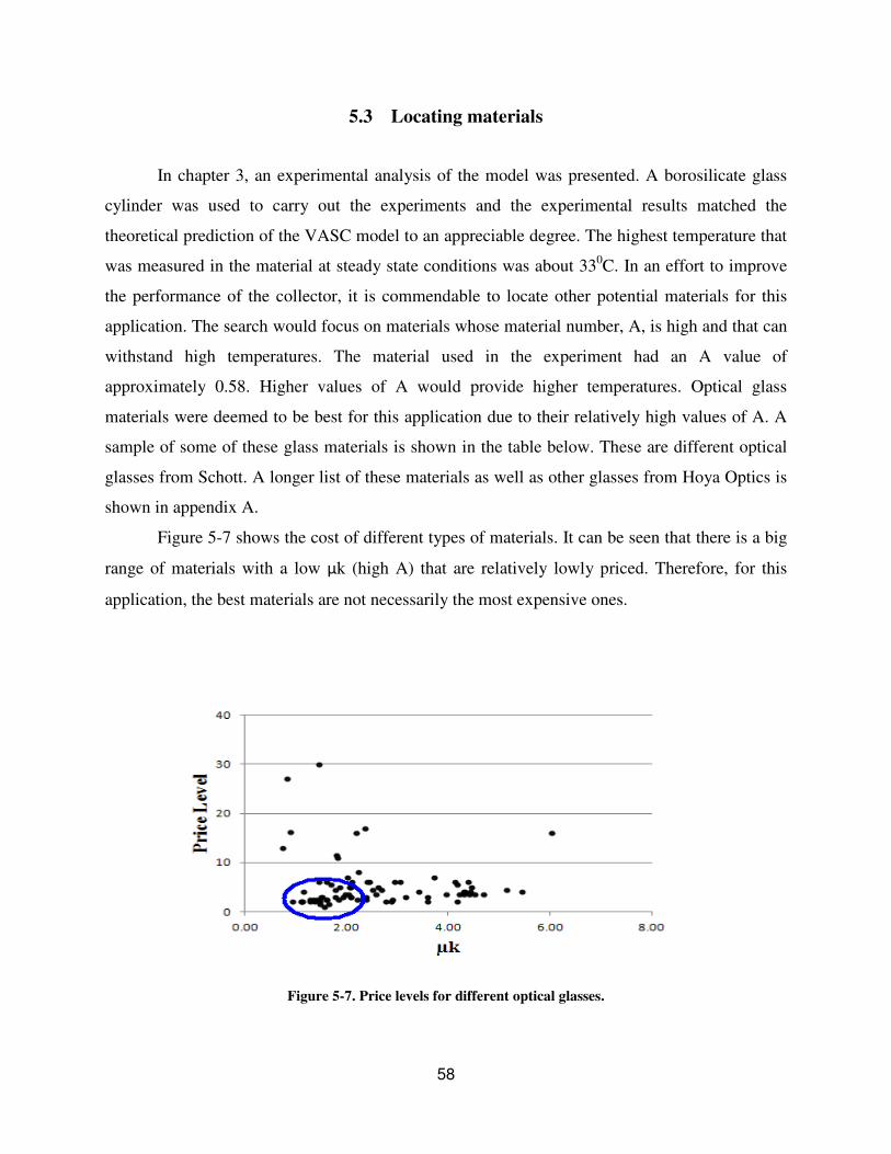
58
5.3 Locating materials
In chapter 3, an experimental analysis of the model was presented. A borosilicate glass
cylinder was used to carry out the experiments and the experimental results matched the
theoretical prediction of the VASC model to an appreciable degree. The highest temperature that
was measured in the material at steady state conditions was about 330C. In an effort to improve
the performance of the collector, it is commendable to locate other potential materials for this
application. The search would focus on materials whose material number, A, is high and that can
withstand high temperatures. The material used in the experiment had an A value of
approximately 0.58. Higher values of A would provide higher temperatures. Optical glass
materials were deemed to be best for this application due to their relatively high values of A. A
sample of some of these glass materials is shown in the table below. These are different optical
glasses from Schott. A longer list of these materials as well as other glasses from Hoya Optics is
shown in appendix A.
Figure 5-7 shows the cost of different types of materials. It can be seen that there is a big
range of materials with a low µk (high A) that are relatively lowly priced. Therefore, for this
application, the best materials are not necessarily the most expensive ones.
Figure 5-7. Price levels for different optical glasses.
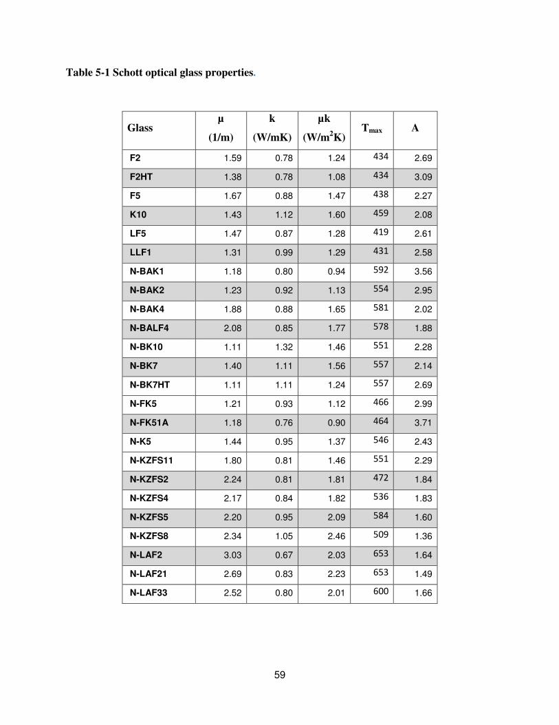
59
Table 5-1 Schott optical glass properties.
Glass µ
(1/m)
k
(W/mK)
µk
(W/m2K)
Tmax A
F2 1.59 0.78 1.24 434 2.69
F2HT 1.38 0.78 1.08 434 3.09
F5 1.67 0.88 1.47 438 2.27
K10 1.43 1.12 1.60 459 2.08
LF5 1.47 0.87 1.28 419 2.61
LLF1 1.31 0.99 1.29 431 2.58
N-BAK1 1.18 0.80 0.94 592 3.56
N-BAK2 1.23 0.92 1.13 554 2.95
N-BAK4 1.88 0.88 1.65 581 2.02
N-BALF4 2.08 0.85 1.77 578 1.88
N-BK10 1.11 1.32 1.46 551 2.28
N-BK7 1.40 1.11 1.56 557 2.14
N-BK7HT 1.11 1.11 1.24 557 2.69
N-FK5 1.21 0.93 1.12 466 2.99
N-FK51A 1.18 0.76 0.90 464 3.71
N-K5 1.44 0.95 1.37 546 2.43
N-KZFS11 1.80 0.81 1.46 551 2.29
N-KZFS2 2.24 0.81 1.81 472 1.84
N-KZFS4 2.17 0.84 1.82 536 1.83
N-KZFS5 2.20 0.95 2.09 584 1.60
N-KZFS8 2.34 1.05 2.46 509 1.36
N-LAF2 3.03 0.67 2.03 653 1.64
N-LAF21 2.69 0.83 2.23 653 1.49
N-LAF33 2.52 0.80 2.01 600 1.66
60
CHAPTER SIX
6 CONCLUSIONS AND RECOMMENDATIONS
The development of solar energy technologies is on a fast track. Today, more than any
other time in history, the potential for the use of solar energy in everyday applications has gained
a lot of attention. A large number of energy companies, even fossil fuel companies, are putting a
lot of effort in developing renewable energy technologies. The BP oil company has one of the
most advanced solar panel. The GE Company is also known to develop solar energy collection
and storage technologies. More solar power plants are being built in California, Spain and around
the world. Irrefutably, there is no turning back from the promise and pursuit of renewable
energies, particularly solar energy.
This work presented a system that would help increase the performance of existing solar
energy collecting technologies. The Volumetric Absorption Solar Collector is based on the same
phenomenon that exists in solar ponds and is governed by the physics of a flat plate collector.
However, the VASC system is thermodynamically superior to both the solar pond and the flat
plate collector, since it has the ability to provide more heat.
A model of the VASC was developed and used to predict the performance of the
collector under different conditions. This model was validated through experimental analysis
using a small semitransparent material, the borosilicate glass. This glass material had a material
number, A, of 0.58. It was shown that the performance of a VASC heavily depends on the value
of A. The higher the value of A is, the greater the collector. Increasing the value of A has
constraints, however, given by the physical properties of the material. Some materials with a
high A value may not be able to handle the temperatures that can be reached during the
application. An ideal medium would be the one with a high transparency, low conductivity and a
high temperature allowance.
One of the potential applications of the volumetric absorption solar collector was
presented and analyzed mathematically. It involved the combination of a VASC with a flat plate
collector. The theoretical analysis showed that the combined system would slightly increase
fixed losses but strongly decrease variable losses, therefore have a greater overall performance.
61
The increase in fixed losses had a negative impact on the combined system for the very low
temperature applications but as the temperature gets higher, this impact was nullified. The
application of a VASC to flat plate collectors is not to be confused with FPC with multiple
covers. When this is done, a significant amount of radiation, 8% per glazing, is lost through
reflection and reradiation. With one thick semitransparent material, the reflective losses are
minimized and the overall performance is improved.
Finally, different materials available on the market deemed to have a good performance
for this application were presented, along with their relative cost. It was found that the best of the
chosen materials are not necessarily the most expensive for this particular application, which
puts the VASC system at a competitive advantage in terms of economics.
In the future, it is suggested that an experimental analysis be done on the VASC-FPC
system that was proposed and analyzed in this work. From the theoretical analysis, it was shown
that for temperatures of approximately 1000C, the combined system can perform at efficiencies
as high as 4 times the efficiency of a normal flat plate collector alone. It would be useful to prove
this assertion through experimental analysis.
The next suggestion for future work is to locate other potential applications for the
volumetric absorption solar collector. Examples of such include the use of the VASC as a
volumetric solar energy receiver for compound parabolic collectors. A theoretical analysis of the
performance of the combined system as well as an experimental analysis would be beneficial.
Even though a wide range of materials were presented, it is suggested that future work on this
topic tries to determine the best material for this application. This would be the material with a
high thermodynamic stability (high transformation temperature), high transmissivity in order to
allow more solar radiation to pass through, and a low thermal conductivity in order to keep much
of the energy received and reduce conduction heat losses.
Finally, it is suggested that a comprehensive economical analysis be done for a VASC
system or a VASC-FPC system or any other application that uses the VASC. This would help
make an informed conclusion about the economic viability of the collector and whether the
added manufacturing costs of this collector are offset by its thermodynamic superiority.
***ENDS***
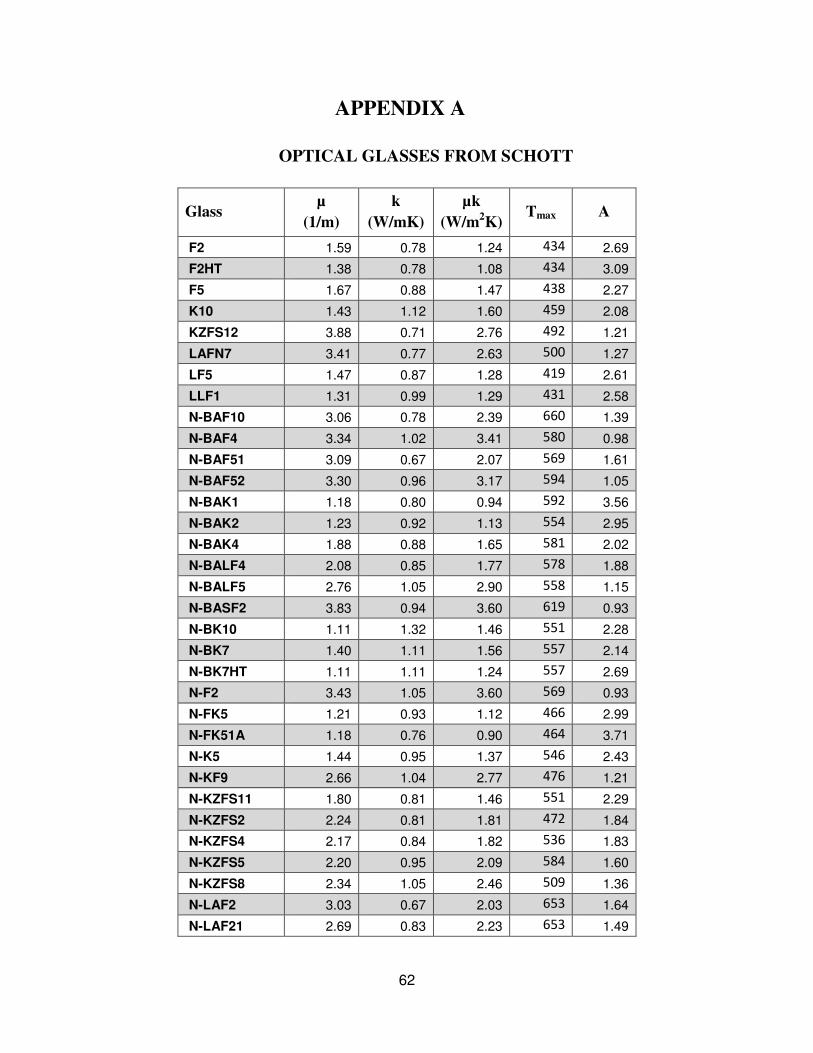
62
APPENDIX A
OPTICAL GLASSES FROM SCHOTT
Glass µ
(1/m)
k
(W/mK)
µk
(W/m2K)
Tmax A
F2 1.59 0.78 1.24 434 2.69
F2HT 1.38 0.78 1.08 434 3.09
F5 1.67 0.88 1.47 438 2.27
K10 1.43 1.12 1.60 459 2.08
KZFS12 3.88 0.71 2.76 492 1.21
LAFN7 3.41 0.77 2.63 500 1.27
LF5 1.47 0.87 1.28 419 2.61
LLF1 1.31 0.99 1.29 431 2.58
N-BAF10 3.06 0.78 2.39 660 1.39
N-BAF4 3.34 1.02 3.41 580 0.98
N-BAF51 3.09 0.67 2.07 569 1.61
N-BAF52 3.30 0.96 3.17 594 1.05
N-BAK1 1.18 0.80 0.94 592 3.56
N-BAK2 1.23 0.92 1.13 554 2.95
N-BAK4 1.88 0.88 1.65 581 2.02
N-BALF4 2.08 0.85 1.77 578 1.88
N-BALF5 2.76 1.05 2.90 558 1.15
N-BASF2 3.83 0.94 3.60 619 0.93
N-BK10 1.11 1.32 1.46 551 2.28
N-BK7 1.40 1.11 1.56 557 2.14
N-BK7HT 1.11 1.11 1.24 557 2.69
N-F2 3.43 1.05 3.60 569 0.93
N-FK5 1.21 0.93 1.12 466 2.99
N-FK51A 1.18 0.76 0.90 464 3.71
N-K5 1.44 0.95 1.37 546 2.43
N-KF9 2.66 1.04 2.77 476 1.21
N-KZFS11 1.80 0.81 1.46 551 2.29
N-KZFS2 2.24 0.81 1.81 472 1.84
N-KZFS4 2.17 0.84 1.82 536 1.83
N-KZFS5 2.20 0.95 2.09 584 1.60
N-KZFS8 2.34 1.05 2.46 509 1.36
N-LAF2 3.03 0.67 2.03 653 1.64
N-LAF21 2.69 0.83 2.23 653 1.49
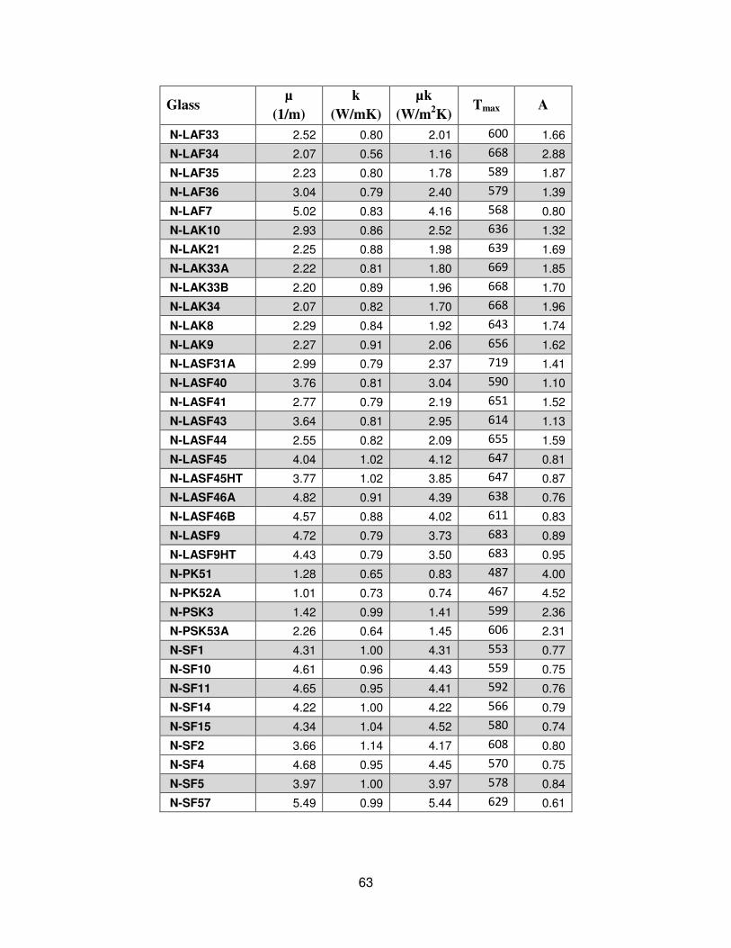
63
Glass µ
(1/m)
k
(W/mK)
µk
(W/m2K)
Tmax A
N-LAF33 2.52 0.80 2.01 600 1.66
N-LAF34 2.07 0.56 1.16 668 2.88
N-LAF35 2.23 0.80 1.78 589 1.87
N-LAF36 3.04 0.79 2.40 579 1.39
N-LAF7 5.02 0.83 4.16 568 0.80
N-LAK10 2.93 0.86 2.52 636 1.32
N-LAK21 2.25 0.88 1.98 639 1.69
N-LAK33A 2.22 0.81 1.80 669 1.85
N-LAK33B 2.20 0.89 1.96 668 1.70
N-LAK34 2.07 0.82 1.70 668 1.96
N-LAK8 2.29 0.84 1.92 643 1.74
N-LAK9 2.27 0.91 2.06 656 1.62
N-LASF31A 2.99 0.79 2.37 719 1.41
N-LASF40 3.76 0.81 3.04 590 1.10
N-LASF41 2.77 0.79 2.19 651 1.52
N-LASF43 3.64 0.81 2.95 614 1.13
N-LASF44 2.55 0.82 2.09 655 1.59
N-LASF45 4.04 1.02 4.12 647 0.81
N-LASF45HT 3.77 1.02 3.85 647 0.87
N-LASF46A 4.82 0.91 4.39 638 0.76
N-LASF46B 4.57 0.88 4.02 611 0.83
N-LASF9 4.72 0.79 3.73 683 0.89
N-LASF9HT 4.43 0.79 3.50 683 0.95
N-PK51 1.28 0.65 0.83 487 4.00
N-PK52A 1.01 0.73 0.74 467 4.52
N-PSK3 1.42 0.99 1.41 599 2.36
N-PSK53A 2.26 0.64 1.45 606 2.31
N-SF1 4.31 1.00 4.31 553 0.77
N-SF10 4.61 0.96 4.43 559 0.75
N-SF11 4.65 0.95 4.41 592 0.76
N-SF14 4.22 1.00 4.22 566 0.79
N-SF15 4.34 1.04 4.52 580 0.74
N-SF2 3.66 1.14 4.17 608 0.80
N-SF4 4.68 0.95 4.45 570 0.75
N-SF5 3.97 1.00 3.97 578 0.84
N-SF57 5.49 0.99 5.44 629 0.61
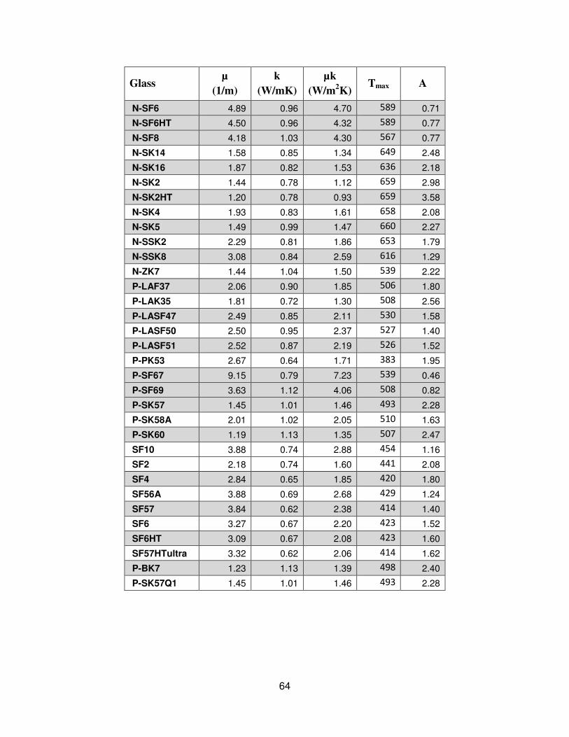
64
Glass µ
(1/m)
k
(W/mK)
µk
(W/m2K)
Tmax A
N-SF6 4.89 0.96 4.70 589 0.71
N-SF6HT 4.50 0.96 4.32 589 0.77
N-SF8 4.18 1.03 4.30 567 0.77
N-SK14 1.58 0.85 1.34 649 2.48
N-SK16 1.87 0.82 1.53 636 2.18
N-SK2 1.44 0.78 1.12 659 2.98
N-SK2HT 1.20 0.78 0.93 659 3.58
N-SK4 1.93 0.83 1.61 658 2.08
N-SK5 1.49 0.99 1.47 660 2.27
N-SSK2 2.29 0.81 1.86 653 1.79
N-SSK8 3.08 0.84 2.59 616 1.29
N-ZK7 1.44 1.04 1.50 539 2.22
P-LAF37 2.06 0.90 1.85 506 1.80
P-LAK35 1.81 0.72 1.30 508 2.56
P-LASF47 2.49 0.85 2.11 530 1.58
P-LASF50 2.50 0.95 2.37 527 1.40
P-LASF51 2.52 0.87 2.19 526 1.52
P-PK53 2.67 0.64 1.71 383 1.95
P-SF67 9.15 0.79 7.23 539 0.46
P-SF69 3.63 1.12 4.06 508 0.82
P-SK57 1.45 1.01 1.46 493 2.28
P-SK58A 2.01 1.02 2.05 510 1.63
P-SK60 1.19 1.13 1.35 507 2.47
SF10 3.88 0.74 2.88 454 1.16
SF2 2.18 0.74 1.60 441 2.08
SF4 2.84 0.65 1.85 420 1.80
SF56A 3.88 0.69 2.68 429 1.24
SF57 3.84 0.62 2.38 414 1.40
SF6 3.27 0.67 2.20 423 1.52
SF6HT 3.09 0.67 2.08 423 1.60
SF57HTultra 3.32 0.62 2.06 414 1.62
P-BK7 1.23 1.13 1.39 498 2.40
P-SK57Q1 1.45 1.01 1.46 493 2.28
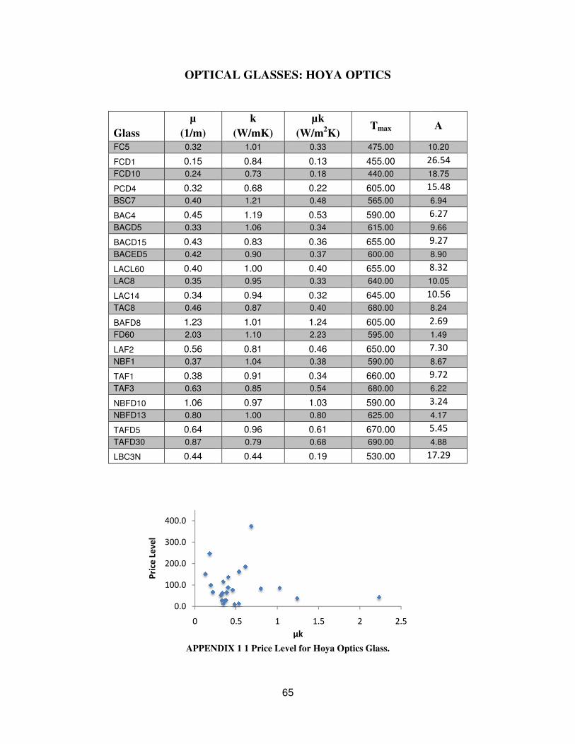
OPTIC
Glass
µ
(1/m)
FC5 0.32
FCD1 0.15
FCD10 0.24
PCD4 0.32
BSC7 0.40
BAC4 0.45
BACD5 0.33
BACD15 0.43
BACED5 0.42
LACL60 0.40
LAC8 0.35
LAC14 0.34
TAC8 0.46
BAFD8 1.23
FD60 2.03
LAF2 0.56
NBF1 0.37
TAF1 0.38
TAF3 0.63
NBFD10 1.06
NBFD13 0.80
TAFD5 0.64
TAFD30 0.87
LBC3N 0.44
APPEN
0.0
100.0
200.0
300.0
400.0
0
Pri
ce L
ev
el
65
ICAL GLASSES: HOYA OPTICS
k
(W/mK)
µk
(W/m2K)
Tmax
1.01 0.33 475.00 1
0.84 0.13 455.00 26
0.73 0.18 440.00 1
0.68 0.22 605.00 15
1.21 0.48 565.00
1.19 0.53 590.00 6.
1.06 0.34 615.00
0.83 0.36 655.00 9.
0.90 0.37 600.00
1.00 0.40 655.00 8.
0.95 0.33 640.00 1
0.94 0.32 645.00 10
0.87 0.40 680.00
1.01 1.24 605.00 2.
1.10 2.23 595.00
0.81 0.46 650.00 7.
1.04 0.38 590.00
0.91 0.34 660.00 9.
0.85 0.54 680.00
0.97 1.03 590.00 3.
1.00 0.80 625.00
0.96 0.61 670.00 5.
0.79 0.68 690.00
0.44 0.19 530.00 17
NDIX 1 1 Price Level for Hoya Optics Glass.
0.5 1 1.5 2 2.5
µk
A
10.20
26.54
18.75
15.48
6.94
6.27
9.66
9.27
8.90
8.32
10.05
10.56
8.24
2.69
1.49
7.30
8.67
9.72
6.22
3.24
4.17
5.45
4.88
17.29
66
REFERENCES
1. World Energy Outlook 2009 Edition, 2009, from http://www.iea.org/weo/2009.asp
2. Barsky, R.; Kilian, L.. 2010, "Oil and the Macroeconomy Since the 1970s," CEPR
Discussion Paper No. 4496 1001: pp. 48109–1220
3. Making Better Energy Choices, n.d, from www.worldwatch.org
4. The Fifth Fuel, n.d., from www.thefifthfuel.com
5. Rivera-Alvarez, A., Londono-Hurtado, A., 2003, “Maximization of Energy Output from Volumetric Absorption Solar Collector,” Journal of Solar Engineering, 125, pp. 83-87
6. Xenophon, 2010, “The Memorable Thoughts of Socrates,” Indo-European Publishing
7. History of Solar, n.d., from http://www1.eere.energy.gov/solar/pdfs/solar_timeline.pdf
8. Yergin, D.,2011, Energy, Security, and the Remaking of the Modern World, The Penguins Press, New York 2011
9. Kalogirou, S.A., 2004, “Solar thermal collectors and applications,” Progress in Energy and Combustion Science, 30 (3), pp. 231–295
10. Smalley, R.E., 2005, “Future Global Energy Prosperity: The Terawatt Challenge,” MRS Bulleting, 30, pp. 412-417
11. Wang, R.Z., Zhai, X.Q., 2010, “Development of solar thermal technologies in China,” Energy, 35 (11), pp. 4407–4416
12. Barlev, D., Vidu, R., Stroeve, P., 2011, “Innovation in concentrated solar power,” Solar Energy Materials and Solar Cells, 95 , pp. 2703–2725
13. Tang, R., Gao, W., Yu, Y., Chen, H., 2009, “Optimal tilt-angles of all-glass evacuated tube solar collectors,” Energy, 34 (9) , pp. 1387–1395
14. Zambolin, E., Del, D., 2010, “Experimental analysis of thermal performance of flat plate and evacuated tube solar collectors in stationary standard and daily conditions,” Solar Energy, 84 (8) , pp. 1382–1396
15. He,W., Su, Y., Wang, Y.Q., Riffat, S.B., Ji,J., 2012, “A study on incorporation of thermoelectric modules with evacuated-tube heat-pipe solar collectors,”, Renewable Energy, 37(1), pp. 142–149
67
16. Chow, T., Dong, Z., Chan, L., Fong, K., Bai, Y., 2011, “Performance evaluation of evacuated tube solar domestic hot water systems in Hong Kong,” Energy and Buildings 43(12), pp. 3467–3474
17. Mahjouri, F., 2011, “Vacuum Tube Liquid-Vapor (Heat-Pipe) Collectors,” http://www.thermomax.com/Downloads/Vacuum%20Tube%20Paper.pdf, Consultado el 10 de Enero.
18. Avila-Marin, A.L., “Volumetric Receivers in Solar Thermal Power Plants with Central Receiver System Technology: A review,” Solar Energy, 85 (2011), pp. 891-910
19. Kribus, A., Ries, H., Spirkl, W., “Inherent Limitation of Volumetric Solar Receivers,” ASME Journal of Solar Energy Engineering, 118, pp. 151-155, 1996.
20. Fend, T., “High Porosity Materials as Volumetric Receivers for Solar Energetics,” Optica Applicata, Vol. XL, No.2, 2010.
21. Incropera, F. P., and DeWitt, D. P., 1996, Fundamentals of Heat and Mass Transfer, 4th Edition, Wiley.
22. Goswami, D. Y., Kreith, F., and Kreider, J. F., 1999, Principles of Solar Engineering, Taylor
and Francis, Philadelphia, PA.
68
BIOGRAPHICAL SKETCH
Philibert Girurugwiro, a native of Rwanda, was born on 12/12/1985 and grew up during
the most violet and tumultuous period of his country’s history. As a refugee in Tanzania, he had
to suspend his education. When he returned home, he completed high school and received a
national award for outstanding performance in science. In 2006, Phil received a Rwandan
Presidential Scholarship to study in the United States. He enrolled at Oklahoma Christian
University, majoring in mechanical engineering. In 2008, he returned home to work in the
energy sector of the Rwandan Ministry of Infrastructure. There he quickly discerned the potential
value of renewable energy to his country’s development. After receiving his BS in engineering
from Oklahoma Christian University in 2010, Phil entered FSU’s Masters Program in
Mechanical Engineering with an emphasis on sustainable energy. At FSU, he also became a
fellow of William Kerr Institute of Intercultural Education and Dialogue. He hopes to acquire the
necessary skills with which to contribute to the advancement of his country’s economy by
reducing its high level of energy dependence.