The Visual Perception of Variation in Data Displays Visual Perception of Variation in Data Displays Stephen Few

Copyright © 2016 Stephen Few, Perceptual Edge Page 1 of 15

Human visual perception has evolved a heightened sensitivity to variation—differences. Our ability to spot even subtle differences between objects in our field of vision, such as between the contours and colors of leaves and that of a tiger crouching behind them, helped set us on the path to evolutionary high ground. Visual perception occurs in the visual cortex of the brain and does so immediately and preattentively, prior to conscious awareness. Approximately 30 separate processes, each designed to perceive a different characteristic of objects that we see in the world (position, size, shape, color, angle, etc.), occur simultaneously in the visual cortex. It is from these individual preattentive attributes of perception that the objects that we see with our eyes are constructed as images in our mind’s eye.

We display quantitative data so that we can examine two characteristics of that data: variation and relationships. In variation we see how values differ from one another and the meaningful patterns formed by those differences across entire sets of values. In relationships between variables we discover how they behave relative to one another, often to understand how they affect one another.

When we display quantitative data, we must design those displays for human perception and cognition. Our designs succeed or fail to the degree that they are aligned with the abilities of human perception and cognition. In this article, I’ll focus on the perceptual aspects of design that affect our ability to examine variation. When we understand visual perception, we can design displays to intentionally tap into preattentive visual processes in ways that can be easily and rapidly perceived. This lays the foundation on which understanding can be built.

The Nature of VariationWhen we attempt to make sense of quantitative data, more than anything else we examine its variation. Quantitative data exhibits several types of variation, such as variation through time or variation in the distribution of values from lowest to highest. We refer to an element of data that varies as a variable. There are two fundamental types of variables: quantitative and categorical.

Quantitative Variables

Quantitative variables are expressed as numbers. Although numbers can be used to express non-quantitative variables, such as a customer number, when numbers can be manipulated mathematically, such as by summing them or finding their average, they are quantitative. Another common name for a quantitative variable is a measure. This is because the quantities express something that has been measured, such as sales in dollars or a person’s height in inches. Quantitative variables describe how much there is of something.

Measures vary along a quantitative range. For example, people’s ages vary from 0—the moment of birth—to a maximum of 100 or so, with a few long-lived exceptions.

Categorical Variables

Categorical variables are qualitative rather than quantitative. They describe what something is, such as what product, what country, or what color. In the realm of information technology, especially data warehousing and business intelligence, another common name for a categorical variable is a dimension. Like quantitative variables, categorical variables consist of values, but the values are qualitative. Because the term value, as ordinarily used, suggests something that is quantitative, I often refer to categorical values as items instead.

The Visual Perception of Variation in Data Displays

Stephen Few, Perceptual EdgeVisual Business Intelligence Newsletter

October/November/December 2016

http://www.perceptualedge.com

http://www.perceptualedge.com/newsletter.php


A categorical variable consists of items that are particular to that category. For example, a category named department in a particular organization might consist of the items sales, marketing, operations, information systems, human resources, and administration.

Examining Quantitative Variation: Two PerspectivesIn the realm of quantitative data analysis (a.k.a., statistical analysis), unlike qualitative analysis, we consider quantitative values even when we’re comparing categorical items. For example, we might want to compare departments to one another based on expenses or the number of employees in each. How we examine quantitative variation depends on the nature of the variable and what we’re trying to understand. At the most fundamental level, we either examine a variable’s overall pattern of variation or differences among individual values. This distinction is important, for it often determines how we design the display. Some data visualizations make it easy to see and compare overall patterns among an entire set of values and others make it easy to see and compare individual values. The two data visualizations below of the same time-series values illustrate this difference:

0

100,000

200,000

300,000

400,000

500,000

600,000

Nov Dec Jan Feb Mar Apr May Jun Jul Aug Sep Oct

Actual vs. Budgeted ExpensesPrevious 12 Months (as of Nov. 1, 2016)

0

100,000

200,000

300,000

400,000

500,000

600,000


Actual vs. Budgeted ExpensesPrevious 12 Months (as of Nov. 1, 2016)

USD

USD

The line graph makes the overall patterns of change easy to see and compare. The bar graph does not support these tasks well at all, but it makes it easy to compare individual actual and budgeted expenses in particular months.

Preattentive Visual Attributes and the Display of VariationSeveral preattentive attributes of visual perception can potentially play a role in displaying data variation on a screen or printed page. Their roles differ, however, in degree and effectiveness. The following is a list of the


preattentive attributes that are most useful, organized into four types: form, color, location, and motion.

Attributes of Form

• Length

• Width

• Area

• Shape

• Angle

• Orientation

• Enclosure

• Blur

Attributes of Color

• Hue

• Lightness

• Saturation

• Intensity

Attributes of Location

• 2-D position

• Spatial grouping

Attributes of Motion

• 2-D direction of motion

• Speed of motion

Before describing their uses for displaying variation, let me clarify what they are.

Length Objects can vary along three dimensions: length, width, and depth. For our purposes, length refers to the primary dimension in which an object varies. For example, in a vertical bar graph, variation along the vertical dimension (a.k.a., height) represents length, but in a horizontal bar graph, variation along the horizontal dimension represents length.

Width Width refers variation along the secondary dimension. For example, in a vertical bar graph, variation along the horizontal dimension represents width, but in a horizontal bar graph, variation along the vertical dimension represents width.

Area 2-D objects that vary along both dimensions (i.e., length and width) are perceived as variations in area, the combination of length and width, rather than independently as length and width.

Shape The forms of objects are their shapes. In graphs, we almost always use simple shapes, such as circles, rectangles, triangles, and lines. Objects can have complex shapes, but their complexity is rarely useful for encoding data because it is too difficult to interpret.

Angle When two lines or two flat surfaces intersect, an angle is formed. The most common occurrence of angles in graphs are formed by slices of a pie chart where they radiate out from the center.


Orientation The direction in which a line or flat surface extends vertically through space (e.g., upwards from left to right, downwards from left to right, or relatively flat from left to right, and to what degree). Slope is sometimes identified as a separate attribute from orientation, but perceptually it is merely orientation in the context of a horizontal baseline. For example, in a line graph, which has a horizontal axis called the X axis, the slope of a line is its orientation relative to the X axis.

Enclosure The presence or absence of a container around data. Enclosure is usually created using a line to form a border around data or using fill color in background to do this.

Blur The clarity vs. fuzziness of a visual image.Hue What we usually think of by the term color. In this context, hue is what we ordinarily mean

by a specific color (red, green, blue, yellow, orange, etc.)Lightness Variation in a color’s brightness, from light to dark.Saturation Variation in a color’s colorfulness, from a lowly-saturated, gray-like version of a color to a

highly-saturated, vibrant version.Intensity Variation in a combination of lightness and saturation, which are perceived integrally, rather

than separately. By combining these two attributes of color, greater perceptual distinctions along a series of colors can be discerned.

2-D position The location of an object on a flat surface, which can be specified as a particular vertical and horizontal position. Cartesian coordinates—encoding locations in relation to a quantitative scale along the X axis and a quantitative scale along the Y axis—are used in graphs to specify 2-D locations.

Spatial grouping The sense that objects form a group based on proximity to one another.2-D direction of motion

The direction in which an object moves on a flat, 2-D plane.

Speed of motion

The speed at which an object moves, regardless of direction.

Perhaps you noticed that 3-D position does not appear in this list. This is intentional. Scientists who study visual perception sometimes refer to human vision as being two and a half dimensional rather than three dimensional. They do this to make the point that our perception of depth, the third spatial dimension, is not nearly as good as our perception of 2-D position (up and down, right and left). This is because we don’t perceive depth directly, but through a combination of other attributes, including area (larger objects appear closer), blur (clearer objects appear closer), occlusion (objects that appear in front of others appear closer), and stereoscopic vision (differences in the view of each eye that vary by distance). Because depth perception doesn’t work very well, it is usually best to avoid its use in data displays. This is especially true when displaying data on a flat surface, such as a screen or a piece of paper, which are limited to two dimensions. Creating the pseudo-appearance of depth on a flat surface uses visual tricks rather than actually varying the distance of objects from the viewer.

Even though all of the attributes in this list can play a role in the display of variation, not all of them can be intentionally applied when designing a data display. For example, in a scatterplot, the fact that a few data points are clustered near one another to form a spatial grouping is meaningful, but it exists because the values are close to one another, not because they were intentionally placed near one another. Some attributes are particularly useful for representing quantitative values and some for associating values with particular categorical items.

Attributes for Encoding Quantitative Values

We perceive attributes that vary along a continuum from less to more, such as length, size, and color intensity, in a quantitative manner. All of the attributes that appear in the list above vary continuously, except for enclosure, which either exists or doesn’t. Just because an attribute varies continuously does not necessarily


mean that we perceive it as ranging from less to more. Hue, for example, varies along a continuum of color measured as frequencies of visible light but we do not naturally perceive some hues as quantitatively greater in value than others. Instead, we merely perceive them as different from one another. Although spatial grouping varies continuously in the sense that groupings can seem more or less dense, this attribute cannot readily be assigned to objects to encode quantitative values.

The attributes that appear in the list below can all be intentionally used to encode quantitative values, but to varying levels of effectiveness:

Attributes of Form

• Length

• Width

• Area

• Angle

• Slope (i.e., orientation in the context of a horizontal baseline formed by the X axis of a graph)

• Blur

Attributes of Color

• Lightness

• Saturation

• Intensity


• 2-D position

Attributes of Motion

• 2-D direction of motion

• Speed of motion

To some extent, the effectiveness of these attributes for encoding quantitative information can be ranked. William Cleveland and John McGill investigated this back in 1985 in a landmark study titled “Graphical Perception and Graphical Methods for Analyzing Scientific Data.” This research continues to inform our understanding today, although some recent studies have refined our understanding a bit.

For our purposes, there is little practical value in ranking all of these attributes. Let me explain. Two of the attributes—2-D position and length—work far better than the others and are similar in effectiveness. Nevertheless, Cleveland and McGill also ranked the other attributes in the following sequence: angle, slope, area, saturation, and lightness (a.k.a., density). They did not test the effectiveness of color intensity—the combination of lightness and saturation as an integrated attribute—but if they had they would have found that it performs better than either lightness or saturation do individually. In my opinion, the degree to which these less useful attributes differ in effectiveness is not significant enough to rely on a ranking as a guide for design choices. Instead, when neither 2-D position nor length can be used to encode quantitative values and another attribute must be selected, the one that works best is usually determined by the situation rather than minor differences in general effectiveness. For example, in a scatterplot, which represents values as individual points, each encoding two quantitative variables—one as its horizontal position relative to the X axis and the other as


its vertical position relative to the Y axis—if we want to add a third quantitative variable to the display, it usually works best to vary the size of the points in the form of a bubble plot.

Because points in a scatterplot are usually small (e.g., dots), approaches that assign visual attributes to those small objects, such as varying the color intensity of the points, would not work as well because they would be difficult to see, illustrated below.

Cleveland and McGill also included hue in their list, which does not appear in mine, but they placed it dead last because it performed poorly, which wasn’t surprising. We don’t perceive different hues quantitatively, from low


values to high, even though they range along a continuum of frequency values, roughly from 400 nanometers (violet) to 700 nanometers (red). If you’ve memorized the frequency values of particular hues, you could put them in order, but we don’t naturally perceive them in this manner. Instead, we perceive hues as different from one another without a particular order. It is for this reason that hues don’t do a good job of representing quantitative values, which is why I’ve excluded hue from the list entirely.

Attributes for Encoding Categorical Values

Even though most of the preattentive attributes in the original list on page 3 can be used with some success in a graph to associate categorical items with quantitative values, the following are most useful:

Attributes of Form

• Shape

• Enclosure

Attributes of Color

• Hue

• Color intensity


• 2-D position

• Spatial grouping

Most of the time, we associate categorical items with objects in a graph by placing them in distinct locations and labeling them. The four examples below illustrate the way this is typically done.

0

200,000

400,000

600,000

800,000

1,000,000

1,200,000

Marcia Ted Leslie Karen Hector Tony

Revenue by Salesperson

500,000

600,000

700,000

800,000

900,000

1,000,000

1,100,000

Marcia Ted Leslie Karen Hector Tony


0 200,000 400,000 600,000 800,000 1,000,000 1,200,000

Marcia

Ted

Leslie

Karen

Hector

Tony


500,000 600,000 700,000 800,000 900,000 1,000,000 1,100,000

Marcia

Ted

Leslie

Karen

Hector

Tony


U.S. Dollars U.S. Dollars

U.S. Dollars U.S. Dollars


Sometimes categorical associations are made using spatial grouping. In the following scatterplot, because the four categorical items, “high-frequency customers,” “high-frequency customers with unusually small orders,” “low-frequency customers,” and “customers with few, unusually large orders,” are associated with the four quadrants of the graph, each spatial group can easily be labeled.

0

5,000

10,000

15,000

20,000

25,000

30,000

0 5 10 15 20 25 30

Revenue per Customer

(U.S. Dollars)

Orders per Customer

High-frequency customerswith unusally small orders

High-frequency customersCustomers with few,unusually large orders

Low-frequency customers

On rare occasions, borders can be drawn around subsets of values in a graph or fill colors can be placed in the background, serving as enclosures to separate them into discrete categorical groups. Ordinarily, this can only be done effectively when enclosing values that are near one another, forming spatial groups. In the following example, categorical groups of points in a scatterplot were near enough to one another to allow distinct borders to be drawn around them.

150

200

250

300

350

400

450

500

550

600

650

0 5 10 15 20 25 30 35 40 45 50

Avg. NightlyRevenue

(U.S. Dollars)

Total Nights Stayed

The Seaside Shanty B&B - Guests in Loyalty Program

Tiers: Silver Gold Platinum


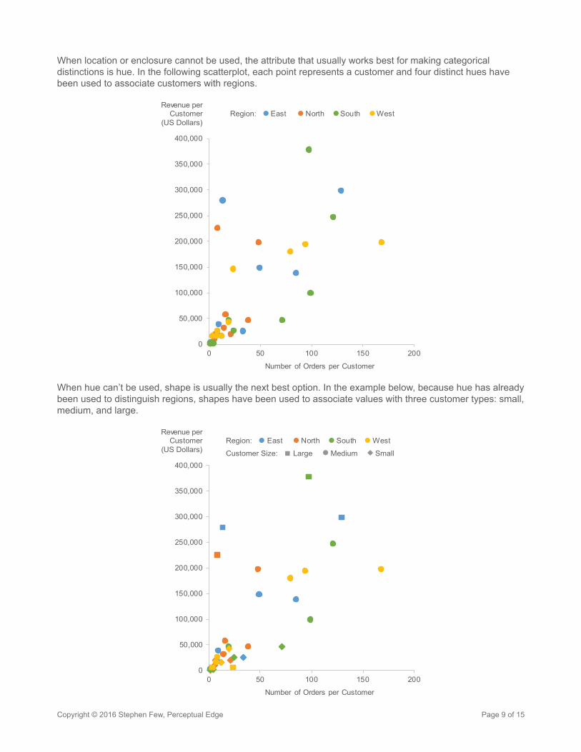
When location or enclosure cannot be used, the attribute that usually works best for making categorical distinctions is hue. In the following scatterplot, each point represents a customer and four distinct hues have been used to associate customers with regions.

0

50,000

100,000

150,000

200,000

250,000

300,000

350,000

400,000

0 50 100 150 200

Number of Orders per Customer

Revenue perCustomer

(US Dollars)Region: SouthNorthEast West

When hue can’t be used, shape is usually the next best option. In the example below, because hue has already been used to distinguish regions, shapes have been used to associate values with three customer types: small, medium, and large.

0

50,000

100,000

150,000

200,000

250,000

300,000

350,000

400,000

0 50 100 150 200


Revenue perCustomer

(US Dollars) Large Medium SmallCustomer Size:

Region: SouthNorthEast West


A good trick to know is that by removing the fill color from objects, leaving only the outlines of their shapes, you can make the shapes easier to discriminate. The example below shows the same data as the one above, but the shapes are now slightly easier to discriminate.

0

50,000

100,000

150,000

200,000

250,000

300,000

350,000

400,000

0 50 100 150 200


Revenue perCustomer

(US Dollars)Region: SouthNorthEast West

Large Medium SmallCustomer Size:

When none of the attributes above can be used, the next best option is usually color intensity, but this only works for up to about five or six intensities. Notice in the graphs below that the set of five color intensities on the left stand out much more clearly as different than the similar set of seven intensities on the right. Color lightness and saturation can be used independently rather than integrated as intensity, but only up to four or five, so intensity is ordinarily the better option.

0

50

100

150

200

250

300

350

400

450

500

0 1 2 3 4 5

YTD Sales(Millions USD)

Avg. Customer Rating

Technology Products by YTD Salesand Avg. Customer Rating

Smartphones Tablets Televisions Desktop PCs Laptops

0

50

100

150

200

250

300

350

400

450

500

0 1 2 3 4 5

YTD Sales(Millions USD)

Avg. Customer Rating

Technology Products by YTD Salesand Avg. Customer Rating

Smartphones TabletsTelevisions Desktop PCsLaptops Digital CamerasSmart Home Products


One slight downside to using color intensity, lightness, or saturation for categorical distinctions is the fact that we naturally perceive them quantitatively—the more intense, dark, or saturated the color, the higher its value—but this meaning isn’t intended when we encode categorical values and can be a bit misleading.

Other attributes can be used for categorical distinctions, such as variations in blur or orientation, but with less effectiveness, so its usually best to save them for situations when better options aren’t available, which is extremely rare.

Visual Objects for Displaying VariationWhen we display quantitative data, we place objects in a graph to represent the values. We associate preattentive visual attributes with those objects to encode their values, both quantitative and categorical. We can display quantitative variation by choosing from a small set of simple objects that encode quantitative values using 2-D position or length, or in a pinch, using area. Rarely do we need any but the following:

• Points: Small circles or polygons that represent values based on their 2-D positon in relation to a quantitative scale along one or both of the axes

• Lines: Typically used to connect a series of 2-D positions to represent a series of values, relative to a quantitative scale along one of the axes

• Rectangles: Usually called bars, and for specific purposes boxes, these vary in length only and represent values based both on their lengths and the 2-D positions of their ends in relation to a quantitative scale along one of the axes

• Areas: Circles or polygons that represent values based on their areas

Technically, in geometry, a point is a dimensionless position in space. In the context of graphs, however, an object without size cannot be seen. For our purposes, therefore, by points we mean small objects that are large enough to be seen with sizes that do not vary. When we assign categorical values to points using colors or shapes, they must be a little larger than would otherwise be necessary to be easily seen and distinguished. Similarly, in geometry a line has only length and position, without width, but in the context of graphs, a line must have some degree of width to be seen.

When points in a graph vary only in 2-D position and not also in area or color, we attend only to their positions. When rectangles vary only in length and not also width, which is conventionally true of bars, we attend only to their lengths and to the positions of their ends. When rectangles vary in both length and width, however, we automatically attend to their areas, not independently to their lengths or widths.

To use objects effectively for quantitative data displays, it’s important that we vary those objects only in ways that correspond to variation in meaning, never gratuitously. When objects vary in color, we look for meaning in that variation. When they vary in hue, we tend to assume the existence of categorical meaning. When they vary in lightness, saturation, or intensity, we tend to assume the existence of quantitative meaning.

When quantitative values are encoded as 2-D positions, and those positions vary vertically, we tend to assume that higher is greater, and when they vary horizontally, we tend to assume that farther to the right is greater. The perception of higher as greater appears to be built into our brains. This might also be true of the perception that farther to the right is greater, but it is more likely that this horizontal perception has been derived from language, which in most cases is written from left to right.

When the positions of objects, either horizontal or vertical, are associated with a categorical scale, our interpretation of those positions switches from quantitative to a categorical association with items along the


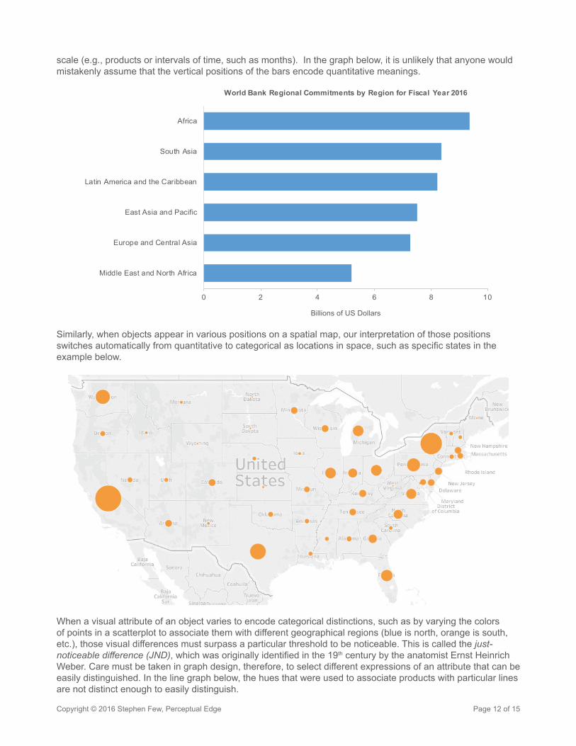
scale (e.g., products or intervals of time, such as months). In the graph below, it is unlikely that anyone would mistakenly assume that the vertical positions of the bars encode quantitative meanings.

0 2 4 6 8 10

Africa

South Asia

Latin America and the Caribbean

East Asia and Pacific

Europe and Central Asia

Middle East and North Africa

Billions of US Dollars

World Bank Regional Commitments by Region for Fiscal Year 2016

Similarly, when objects appear in various positions on a spatial map, our interpretation of those positions switches automatically from quantitative to categorical as locations in space, such as specific states in the example below.

When a visual attribute of an object varies to encode categorical distinctions, such as by varying the colors of points in a scatterplot to associate them with different geographical regions (blue is north, orange is south, etc.), those visual differences must surpass a particular threshold to be noticeable. This is called the just-noticeable difference (JND), which was originally identified in the 19th century by the anatomist Ernst Heinrich Weber. Care must be taken in graph design, therefore, to select different expressions of an attribute that can be easily distinguished. In the line graph below, the hues that were used to associate products with particular lines are not distinct enough to easily distinguish.


3

4

5

6

7


Millions ofUS Dollars

Monthly Men's Shoe Sales by Product NamePrevious 12 Months (as of Nov. 1, 2016)

Kick Me

Honcho

Segall

Rexall Boots

Charles Q's

Boulderdash

Livre

Morado

Maxwell Brown

Excelsior

The graphs that commonly encode values using these objects are illustrated below:

Points Dot plotScatterplot

Lines Line graphFrequency polygon

Rectangles Bar graph (both vertical and horizontal)Box plot (both vertical and horizontal)

Areas Bubble plotBubbles on a mapTreemap

In geospatial displays, quantitative values can be directly assigned to regions of space (e.g., individual states in the United States) without using one of these objects, but by directly filling the regions with colors that vary in intensity (see below). This technique is called a choropleth map.


One other exception to the use of these objects is a heatmap matrix, which is a tabular arrangement that forms rectangular cells at the intersection of each column and row that can be filled with colors of varying intensity to encode quantitative values. In a heatmap matrix, the rectangles do not vary in length or in area to encode quantitative information, but merely serve as placeholders for colors to convey that information.


You might have noticed that areas formed by pie slices were not included in the examples above. This is because pie charts do not display quantitative variation effectively. (For more information on this topic, see the article “Save the Pies for Dessert.”) A few other graphs that you might have encountered were also excluded from the list because they fail to work effectively (e.g., mosaic plots). And finally, a few graphs were excluded from the list, not because they aren’t effective, but because they primarily display relationships among items rather than variation among quantitative values, which falls outside the scope of this article. These include network diagrams and Sankey diagrams.

Final ThoughtsWe can only display quantitative variation effectively if we understand visual perception. Without understanding how humans perceive the world visually, we cannot design displays that work for the human brain. This article does not cover the topic exhaustively. Instead, it provides an introduction to the most important perceptually-based considerations, which can serve as a set of guidelines for design decisions. By following these guidelines, you can display quantitative variation accurately and accessibly. Only after understanding these guidelines through study and practice can you learn to bend them in useful ways.

Discuss this ArticleShare your thoughts about this article by visiting the The Visual Perception of Variation in Data Displays thread in our discussion forum.

About the AuthorStephen Few has worked for over 30 years as an IT innovator, consultant, and teacher. Today, as Principal of the consultancy Perceptual Edge, Stephen focuses on data visualization for analyzing and communicating quantitative business information. He provides training and consulting services, writes the quarterly Visual Business Intelligence Newsletter, and speaks frequently at conferences. He is the author of four books: Show Me the Numbers: Designing Tables and Graphs to Enlighten, Second Edition, Information Dashboard Design: Displaying Data for at-a-Glance Monitoring, Second Edition, Now You See It: Simple Visualization Techniques for Quantitative Analysis, and Signal: Understanding What Matters in a World of Noise. You can learn more about Stephen’s work and access an entire library of articles at www.perceptualedge.com. Between articles, you can read Stephen’s thoughts on the industry in his blog.

http://www.perceptualedge.com/articles/visual_business_intelligence/save_the_pies_for_dessert.pdf

http://www.perceptualedge.com/newsletter.php

http://www.perceptualedge.com/library.php

http://www.perceptualedge.com/blog

http://sfew.websitetoolbox.com/post/the-visual-perception-of-variation-in-data-displays-8315794?pid=1294010341

Documents

The Visual Perception of Variation in Data Displays Visual Perception of Variation in Data Displays Stephen Few