Why Development Levels Differ: The Sources of Differential Economic Growth in a Panel of High and Low Income Countries*

Charles R. Hulten University of Maryland and NBER

and

Anders Isaksson

United Nations Industrial Development Organization (UNIDO) September, 2007

National Bureau of Economic Research Working Paper 13469

(revised)

ABSTRACT: Average income per capita in the countries of the OECD was more than 20 times

larger in 2000 than that of the poorest developing countries. Two general explanations have been

offered to account for the gap: one view stresses the role of the efficiency of production, while a

competing explanation gives primary importance to capital formation. Based on data for 112

countries over the period 1970-2000, we find that differences in the efficiency of production are

the dominant factor accounting for the difference in development levels, and that the gap is likely

to persist under prevailing rates of saving and productivity change.

* The views expressed in the paper are solely those of the authors and do not necessarily reflect the position of UNIDO or any other organization with which the authors are affiliated. We would like to thank the participants at the NBER Summer Institute 2006, as well as Nobuya Haraguchi, for helpful comments and suggestions. Any remaining errors are our own."

1

Why Development Levels Differ: The Sources of Differential Economic Growth in a Panel of High and Low Income Countries

The question of why economic growth differs among countries question has been asked

over and over again, with increasingly better data and ever more sophisticated analytical

techniques.1 However, the answer remains elusive despite the many advances and growing

insights into the problem. Average income per capita in the countries of the OECD was more

than 20 times larger in 2000 than that of the poorest countries of sub-Sahara Africa and

elsewhere, and many of the latter are not only falling behind the world leaders, but have even

regressed in recent years.2 At the same time, other low-income countries have shown the

capacity to make dramatic improvements in income per capita.

Two general explanations have been offered to account for the observed patterns of

growth. One view stresses differences in the efficiency of production are the main source of the

observed gap in output per worker, which is the main source of income per capita. At the heart

of this view is the idea that improvements in technology and the organization of production lead

to higher levels of total factor productivity (TFP) in countries with institutions that support

innovation and promote economic efficiency, along with factors like favorable geography,

1 This question is the organizing theme of the 1998 volume by David Landes “The Wealth and Poverty of Nations.” Landes examines the historical and institutional context of the income disparities that are so apparent today, and describes many of the theories and perceptions that accompanied the emergence of this gap. All research on this issue owes a great debt to the pioneering work of Simon Kuznets, both for his historical insights and for his contributions to the development of the national accounting data that make quantitative analysis possible. The sources-of-growth analysis emerged from this effort, greatly advanced by Solow (1957), and applied international growth by Edward F. Denison (1967) and Maddison (1987). 2 These estimates are based on the country groupings shown in the appendix to this paper, and the data on income per capita in derived from the Penn World Tables (Heston, Summers and Aten, 2002).

2

climate, and political stability. Lower levels of TFP are associated with institutions that inhibit or

retard innovation and the diffusion of technology, or which have unfavorable environmental

factors. In either case, differences in the level of TFP, and not differences in capital formation,

largely explain observed differences in income per capita in this view. 3

A competing explanation reverses this conclusion and gives primary importance to

capital formation. In this paradigm, capital is defined broadly to include human and knowledge

capital, infrastructure systems, as well as the traditional categories of structures and equipment.

TFP differences among countries are thought to be extinguished by the rapid diffusion of

knowledge, and many papers in this branch of the literature then assume that technology is the

same in every country. Some papers also treat technology growth as largely endogenous via

investments in knowledge and human capital, and stress the role of the associated externalities.

To the extent that institutional differences play a role in explaining the income gap, they tend to

be expressed through the rate of capital formation.4

3 See Hall and Jones (1999), Klenow and Rodriguez-Clare (1997), and Easterly and Levine (2001) for recent examples of this approach, and for reviews of the literature. Bosworth and Collins (2003) also provide an extensive survey of recent work in this area, though their own empirical work focuses on rates of growth rather than productivity levels. Contributions to the measurement of international difference in the TFP levels were made by Dowrick and Nguyen (1989), while Färe et al (1994) is an important paper that uses Data Envelopment Analysis to measure technical efficiency (relative to best-practice) among countries. The translog index number approach used in this paper was developed by Jorgenson and Nishimizu (1978), Christensen, Cummings, and Jorgenson (1981), and Caves, Christensen, and Diewert (1982a, 1982b). 4 This literature is somewhat diverse. It includes Mankiw, Romer, and Weil (1992) and the other papers in what Klenow and Rodriguez-Clare (1997) term the “Neoclassical Revival.” See, also, Gollin (2002) for an argument supporting this view. Some of the AK endogenous growth models also fit into this category.

3

The apportionment of the income gap between capital formation and TFP is ultimately an

empirical issue. However, this issue has not proved easy to resolve, in part because of parallel

disputes about which theoretical models of growth are appropriate, the chief protagonists being

endogenous growth theory and neoclassical growth theory. There is also a question of whether it

is differences in the rate of growth of output per worker or the corresponding levels that should

be explained, and, with respect to the latter, the measurement of the TFP gap using Hicksian

versus Harrodian measures of technical change. Not surprisingly, a reading of the literature

reveals that different assumptions and methods give different results, and one goal of this paper

is to examine just how large the difference is for a sample of high and low income countries over

the period 1970 to 2000. Our procedure is to decompose the growth rate of output per worker

into its TFP and capital-deepening components using competing methods, and compare the

results. We follow a similar procedure for the corresponding levels of output per worker, which

we also decompose into TFP and capital-deepening components. We then carry out a similar

decomposition for the Solow steady-state growth model, in order to examine whether the current

gap in output per worker between rich and poor countries is likely to persist into the future given

current parameters and policies, or whether the process of convergence can be expected to

significantly narrow the gap.

The second goal of this paper is to examine the problem of data quality. If there is a

dispute about the size of the TFP gap between rich and poor countries, there can be little doubt

about the corresponding gap in the data quality. Low-income countries tend to have large non-

market sectors for which data are problematic or non-existent, and a market sector with a large

family business component in which labor income can appear as profit. One result is an

implausibly low share of income attributed to labor in national income statistics of some of these

4

countries: labor’s share averages around 30 percent of income in the poorest countries in the

sample of this paper, compared to 50 to 60 percent in the richest. Income shares typically serve

as proxies for the corresponding output elasticities, which in turn are key determinants of the

growth path in most models in the literature (generally, the larger the share of capital, the more

important capital formation is relative to TFP as a source of growth). As a result, many

researchers reject the published data and either estimate the shares using econometric techniques

using the assumption that the shares are constant over time and the same for all countries, or

impose an external estimate of the labor and capital shares, typically around two-thirds and one-

third. These procedures essentially imply that every country has a Cobb-Douglas production

function, which are identical up to a scalar multiple which is associated with the level of TFP

(which is also assumed to be the same for all countries in some formulations). There is a certain

irony in this situation, in view of the debate over the extent to which the variation in output per

worker is due to differences in technology versus differences in capital formation. One objective

of this paper is to reexamine the implications of the two-thirds/one-third share rule and

robustness of the various growth decompositions to changes in this rule.

II. Empirical Growth Modeling

The diverse models in the empirical growth literature share certain common features that

can be used to classify and compare them. One core assumption is that the production

possibilities of an economy can be characterized by a stable aggregate production function (or a

variant of the production function like the cost function or the factor demand equations). Since

many of the differences in the literature can be traced to variations on this theme, we will attempt

to organize the various dimensions of the growth debate using this production framework. Since

5

the discussion is largely about fundamentals, we will use a simple graphical exposition adopted

by Solow in his seminal paper on the sources of growth.

A. The Aggregate Production Function

The aggregate production function relates aggregate output (Y) to total inputs of labor (L)

and capital (K), with allowance for improvements in the productivity of these inputs. This

formulation is so widely used that its implications have become almost invisible in the analysis

of growth. However, it is important to acknowledge that any analysis based on the aggregate

production function asserts, in effect, that the complex technologies of the various firms and

sectors that make up an economy can be summarized accurately by a single functional

representation. The difficulty, here, is that the technical conditions for consistent aggregation are

so restrictive as to be intuitively implausible (see, for, example, Fisher (1965,1969)). Thus, the

use of the aggregate production functions can only be justified as a useful parable for organizing

the data in a way that makes economic sense, and as a framework for interpreting empirical

results. The debate in the literature over which specification of the aggregation production

function is ‘factually’ appropriate for the analysis of cross-national income differences must

therefore be viewed accordingly.

Technical change can be introduced into the aggregate production function in different

ways, but the most common are variants of the model in which the production function is written

as Yt = F(Kt,Lt,t). The time index t allows the production function to shift over time in order to

capture improvements in the efficiency with which the inputs are used, and ‘technical change’ is

conventionally defined as the partial derivative of F(Kt,Lt,t) with respect to t. In the special case

in which technical change augments both input proportionately, the production function has the

6

Hick’s-neutral form Yt = AtF(Kt,Lt). This is the most common form used in empirical growth

accounting, following Solow (1957).

Under the assumption of constant returns to scale, the Hicksian production function can

be expressed in ‘intensive form’ as yt = AtF(kt), with the variables expressed relative to labor: yt

= Yt/Lt and kt = Kt/Lt. This form provides an explicit decomposition of output per worker, yt,

into the two effects of interest, the level of TFP, At , and the capital-deepening effect, F(kt). The

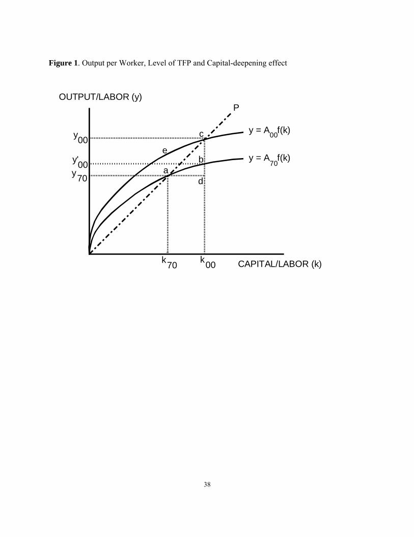
standard graphical representation of the production model is shown in Figure 1. This figure

portrays an economy initially located at the point a on the production function prevailing in that

year (1970 in this example). An increase in the efficiency index, from A70 to A00 in the year

2000, causes the production function to shift upward as in the figure. This is often associated

with the adoption of better technologies over time, but it actually represents a costless

improvement in the effectiveness with which capital and labor are used, and it is more

appropriately characterized as a change in TFP.5

Output gets a further boost, in Figure 1, from an increase in the capital-labor ratio from

k70 to k00. Because of diminishing returns to capital, the production function is shown with a

concave shape. Each increment of capital per worker yields a proportionately smaller increase in

output per worker. With technology held constant, this increase is represented by the move from

point a to point b on the lower A70 branch of the production function. The total change in output

per worker in Figure 1 is from y70 to y00, that is, from point a to point c, and is the sum of the 5 TFP excludes the systematic development of technology paid for by R&D expenditures, but includes the part resulting from R&D externalities, learning, or pure inspiration. In addition, it includes changes in organizational efficiency, and institutional factors such as the legal and regulatory environment, geographic location, political stability, as well as deeper cultural attitudes that affect the work place. It also sweeps in all other factors not explicitly included in measured input: omitted variables like infrastructure capital, variations in the utilization of capital and labor (e.g., unemployment), and measurement errors (for further discussion, see Barro (1999) and Hulten (2001)).

7

capital deepening effect, from point a to point b, and the TFP effect, from point b to point c. The

relative size of these two effects is the point at issue in the capital versus efficiency controversy,

and Figure 1 provides a framework for interpreting and measuring the two effects.

B. Levels versus growth rates

The empirical growth literature provides two ways to implement the intuition of Figure 1,

one based on growth rates (growth accounting) and the other on levels (development

accounting). The answers can be very different, as the following example illustrates. Suppose

that there two economies, A and B, that both start with the same capital-labor ratio, k70.

However, A and B have different levels of output per worker, because they start with different

levels of productive efficiency, that is, Economy A is on the higher of the two production

functions in Figure 1 at point e, and economy B on the lower one at point a. Suppose that, from

this starting point, both economies only grow by capital deepening, which proceeds at the same

rate of growth. They then move along their respective production functions at the same rate, but

neither experiences any growth in productivity (neither function shifts). In this example, the

growth rate in output per worker is due entirely to capital deepening, but all the difference in the

level of output per worker is due to the different level of productive efficiency. Moreover,

economy B may become richer over time, but will never narrow the gap with economy A.

This simple example illustrates the insufficiency of studying comparative growth rates in

isolation from the corresponding levels. Studying comparative levels at a given point in time is

also insufficient, since it cannot indicate the growth dynamics and future prospects of the rich

and poor countries.

8

C. Econometrics versus Nonparametrics

A number of different estimation procedures have been used in empirical growth

analysis. Some studies use an econometric approach in which the production function in Figure

1 is given an explicit functional form and the parameters of that form are estimated.6 Flexible

functional forms like the translog and generalized-Leontieff forms are common in pure

production function studies (or dual cost function and factor demand studies), but are not entirely

suitable for the study of low-income countries, which tend to have both inadequate and

incomplete data. The Cobb-Douglas form Yt = A t Kt" Lt

$ is often used, either explicitly or

implicitly.

Direct estimation of the production function suffers from another well-known problem.

The production function is only one equation in a larger system that determines the evolution of

the system. Kt is determined endogenously in the larger system through the savings/investment

process, and direct estimation can lead to simultaneous equations bias. The use of instrumental

variables is one way to deal with this problem, while another approach is to estimate the reduced

form of the growth system. This second option is the used in Mankiw, Romer, and Weil (1992)

to estimate the parameters of a Cobb-Douglas function indirectly from the reduced form of the

Solow (1956) growth model.

However, both approaches have their drawbacks (e.g., it is difficult to find good

instruments) and nonparametric techniques provide an alternative. The two main alternatives are

the Solow (1957) growth-accounting model and the Data Envelopment Analysis approach,

6 The specification of the error structure of the production function is also an important issue in the growth and production literature. The common approach is to assume an i.i.d. error structure, which is symmetrically distributed around the production function. An alternative approach is to use a one-sided error term, which then allows the error to be associated with departures from the efficiency frontier.

9

although the former (as extended by Jorgenson and Griliches (1967)) is much more widely used

in the growth analysis. The Solow model provides an accounting framework, based on the

Divisia index, in which the growth rate of output per worker (yt) is equal to the growth rate of

capital per worker (kt) weighted by capital’s income share in GDP, plus a residual factor that

accounts for all the remaining growth in yt not explained by the weighted growth of kt.7 Solow

shows that, under the assumption that prices are equal to marginal costs, the income shares are

equal to output elasticities, and the share-weighted growth rate of kt is associated with the

movement along the production function from a to b in Figure 1, i.e., with capital deepening, and

the residual is associated with the shift in the production from b to c. The Solow sources-of-

growth decomposition thus provides a method of resolving the growth rate of yt into the capital-

deepening effect and the TFP effect.

The non-parametric growth accounting approach was extended to the analysis of growth

rate to the analysis of the corresponding levels by Jorgenson and Nishimizu (1978), and

developed by Caves, Christensen, and Diewert (CCD, 1982a). The CCD model is a Törnqvist

index of the level of productivity in each country relative to the average of all countries. It

measures the TFP of any country, relative to the average of all countries, by comparing the

percentage deviation of yt from its international mean with the percentage mean deviation of kt,

weighted by the average of the country’s own income share and the international average.

Because deviations are computed relative the average of all countries, the frame-of-reference

problem implicit in using any one country as the base is avoided. The result is a non-parametric

7 Since accounting data do not come in a continuous time format, the discrete time Törnqvist approximation is typically used in the actual calculations. Growth rates are approximated by the change in the natural logarithms of the variables, weighted by the average income share from one period to the next.

10

decomposition of the relative gap in yt between into its TFP level and capital deepening

components, which complement the sources-of-growth rate analysis.8

D. Hicks versus Harrod neutrality.

The concept of productivity underlying the Solow residual in one in which a given

amount of capital and labor become more productive. The combination k00 Figure 1 yield more

output as a result of the shift in the production function, measured vertically at that capital-labor

ratio. However, like the econometric approach, this non-parametric approach also suffers from a

form of simultaneous equations bias because of the endogeneity of capital. This bias arises from

the fact that a shift in the production function at a given capital-labor ratio leads to an increase in

output per worker and some of this extra output is saved, leading to more output, more saving

and so on. This “induced accumulation effect” is a consequence of TFP growth and should be

attributed to TFP when assessing the importance of productivity change as a driver of growth

(Hulten (1975)).9

The induced accumulation effect can be captured by measuring the shift in the production

function along a constant capital-output ratio, rather than at a constant capital-labor ratio. This

idea, which can be traced back to Harrod (1948), is represented in Figure 1 by the movement

along the pay from the origin (OP) from a to c. It is clear from this figure that all of the growth

in output is accounted for by the shift in the production function, measured along the constant

K/Y ray. However, since the Harrodian gap is measured along a given K/Y ratio, it is not a pure

8 The non-parametric and functional-form approaches are operationally separate, but Diewert (1976) shows that in order for the Törnquist index to be an exact representation of the technology, there must exist an underlying production function of the translog form. This parallels the result by Hulten (1973) that there must be an underlying Hicksian production function in order for the Solow-Jorgenson-Griliches index of TFP to be path independent. 9 See, also, Rymes (1971) and Hulten (1979).

11

measure of the efficiency with which existing resources are used (the normal conception of

productivity). Thus, it does not measure a country’s distance to the best-practice technology

frontier, nor the difference in the technological opportunities separating two countries. It does,

however, measure the consequence of a country’s move to a higher level of technology.

These two approaches measure the shift in a technology along different paths, and can be

implemented for a neoclassical technology of the general form F(Kt,Lt,t), without any special

assumptions about the “neutrality” of the technology. When the shift in the production function

happens to be Hicks neutral, “technical change” augments both marginal products of capital and

labor equally, and the production function has the form Yt = AtF(Kt,Lt). This is the case

assumption in Solow’s 1957 formulation, and it amounts to assuming that the shift in the

technology is invariant to the choice of the capital-labor ratio along which the vertical shift is

measured (e.g., the proportional shift in the production function in Figure 1 is the same the point

a and b). This is the case in which the residual has the property of path independence.

The shift in the production function can also be Harrod neutral (or both, in the Cobb-

Douglas case in which the elasticity of substitution between capital and labor is equal to one). In

this case, Harrodian rate and bias of technical change are evaluated at a constant marginal

product of capital, which, in effect, measures the shift in the production function along the

constant K/Y ratio when the Harrodian bias is zero. 10 This case can be parameterized with a

production function that exhibits labor-augmenting technical change, Yt = F(Kt,atLt).

The Hicksian formation has traditionally been assumed for purposes of measuring the

Solow residual, and the Harrodian approach for steady-state growth theory (though the papers by

10 The essay by Solow (1967) provides a succinct summary of the definitions and interrelations among the various concepts of neutrality and bias, including what subsequently came to be known as Solow neutrality and bias.

12

Klenow and Rodriquez-Care (1997) and Hall and Jones (1999) both apply the Harrodian

convention to TFP measurement, as does Hulten and Nishimizu (1980)). A Solow residual can

be calculated under either assumption, but only with the Hicksian form of neutrality does the

residual retrieve the shift parameter At (given the other assumptions about competition and

returns to scale). When the shift in the production function is Harrod neutral, the Solow

Hicksian residual retrieves the labor-augmenting parameter at when divided by labor’s share of

income. The index formed by dividing TFP by labor’s share is not path independent except in

the Cobb-Douglas case.11 In any case, the analyst has to decide before-hand which form of

neutrality to impose on the problem, which, from the practical standpoint, is a decision about

whether or not to divide the TFP residual by labor’s income share.

This choice has to be made in light of the near certainty that the shift is neither Harrod

nor Hicks neutral (consider the capital-augmenting technical change associated with the

revolution in information technology). Moreover, from the standpoint of measuring the

induced-accumulation effect, no specific form about neutrality is needed.12 This effect can be

captured by measuring the shift in the production function along the K/Y ray through the initial

point (y0, k0), regardless of the assumption about neutrality. Indeed, both the Hicksian and

Harrodian forms of the residual can be computed from the same set of data. The former is useful

11 In the labor-augmenting case, Yt = Kt

" (atLt$), which can be written as Yt = at

$ Kt" Lt

$. The Solow residual is then equal to β time the growth rate of at. The Hicks-neutral form Yt = A t Kt

"

Lt$ gives a Solow residual equal to the growth rate of A t. With the Cobb-Douglas form, labor’s

share of income is constant at β, making both forms path independent. In general, labor’s share is variable, so only the Hicksian form is path independent. 12 For example, if the actual equilibrium point y00 in Figure 1 were to lie somewhere to the right of c, the shift in the Harrodian shift would still be measured along the line P from a to c, regardless of the underlying technology. In this case, the increase in y00 beyond c would be attributed to autonomous capital formation, even though technical change is Harrod-biased.

13

for measuring the “technological distance” between the old and the new levels of technology, in

the sense of the additional output that the old level of factor inputs could produce because of the

new level of technology. This is particularly important for cross-sectional studies comparing

countries at different levels of economic development, where the question of the distance to the

best-practice frontier is highly relevant. The Harrodian approach is useful for addressing the

question of how much of the observed growth in output per worker is the result of the shift in the

technology, inclusive of the induced accumulation effect. Because they address different

questions, neither approach is inherently better than the other.

E. Endogenous Growth

Capital is not the only growth factor that is endogenous. Much of technical innovation is

the result of systematic investments in education and research, and is thus part of overall

(endogenous) capital formation. Moreover, in the framework developed in Lucas (1988) and

Romer (1986), investments in education and research generate spillover externalities. These

externalities may be sufficiently large that growth becomes endogenously self-sustaining,

yielding the “AK” version of the model.

All the growth rate of output is due to capital formation in the pure AK model, and the

sources-of-growth analysis would attribute all of output per worker to capital, both in the rate of

change and the level. However, this presumes that the extent of the externality is known. When

it is not, and this is the normal case when growth-accounting data are derived from observed

market transactions, it is not hard to show that the Solow residual measures the externality

component of capital’s contribution.13 The TFP residual now registers the externality effect, and

14

TFP is reinterpreted accordingly. By implication, differences in the growth rates and levels of

TFP across countries are explained by externalities and driven by capital formation.

F. Steady-State Growth Models

The decompositions discussed thus far provide a backward-looking diagnosis of

economic growth performance and its causes. Past performance is certainly a guide to the

economic future, but it is not sufficient for forecasting the path ahead. It may be the case that a

current income gap exists between two countries, but if they are converging to the same steady-

state level of output per worker, their long-run economic futures will be the same. On the other

hand, if one country is on a higher level of technology than another, both now and in the future,

there will continue to be an income gap despite the convergence of kt to its steady-state path.

To study where countries are heading in the future requires a model that specifies more

that just the production function, since the evolution of capital, labor, and technology must also

be specified. The most fully developed empirical model that fits these requirements is the

Mankiw, Romer, and Weil (1992) – henceforth MRW – model of neoclassical steady-state

growth. MRW start with an augmented version of the Solow (1956) steady-state growth model

and assume that all countries have the same Cobb-Douglas production function. They then solve

the Solow model for its reduced form, which makes steady-state output per worker, y*, a

function of the following variables and parameters: the rate of saving in each country, σi, the

rate of growth in the labor force, ηi, the depreciation of capital, δ, and the Harrodian rate of

13 Barro (1999) analyzes the case where yt = A0kt

γ ktα. The Solow residual is based on the

formulation yt = At ktα, implying that the TFP level index is At = A0kt

γ. In other words, TFP growth is entirely a function of capital formation in a pure endogenous growth situation. Conceptually, the apparent shift in the neoclassical production function is the result of the spillover externality. Endogenous growth theory can therefore be regarded as supplying one rationale for the shift in the production function, a shift that has been termed ‘a measure of our ignorance’ by Abramovitz (1956).

15

technical change, λ. MRW then observe that actual output per worker, yt, converges to the

steady-state value according to an error-correction process that involves the rate of convergence.

They proceed to use their reduced form equation to estimate the Cobb-Douglas output

elasticities, α and β, and the rate of convergence to steady state.

This approach is useful for the current purpose of decomposing steady-state output per

worker into its long-run technology and capital formation components. The left-hand variable,

y*, can be estimated for each country given estimates of σi, ηi, δ, λ, as well as estimates of the

elasticities α and β using income shares. The estimated y* is the level of output per worker

toward which the actual level at any point in time, yt, is converging. Like yt, the estimated y*

must necessarily satisfy the production constraint, y* = A0(k*)α, where k* is the steady-state

value of capital per worker. This permits a simple decomposition of yt into the steady-state level

toward which it is converging, y*, and the gap between the two (which measures the opportunity

for growth due to convergence). Beyond this, the steady-state income gaps between any two

countries, or groups of countries, can be decomposed into a capital-deepening effect and a

Harrodian TFP effect. We carry out both types of level comparison in the empirical section

which follows.

III. Data and Empirics

The various theoretical approaches reviewed in the preceding section present a rich set of

options for empirical work. They also present a challenge, because they offer different views

and competing estimates of the same underlying growth process. We will explore, in this

section, just how much the competing estimates differ. We start with the neoclassical sources-

of-growth model and the Hicksian convention for measuring TFP. This is by far the most

common approach in the empirical growth literature and the one with the largest body of results.

16

A. The Data Sources and Data Problems

The sources-of-growth framework requires times series data on real output, labor input,

capital stocks, and labor’s share of income. These data are constructed for a total of 112

countries over the period 1970-2000. The list of countries, along with selected statistics, is

shown in Table A.1 of the Data Appendix. In order to facilitate comparison, these countries are

grouped into six ‘meta’ countries, mainly based on the World Bank classification by income per

capita (not output per worker, which is highly correlated but not identical). The 40 Low Income

countries are located in Africa, with eight exceptions. The 22 Lower-Middle Income countries

are developing economies spread throughout the world, as are the 17 Upper-Middle Income

countries. The 24 High-Income countries are basically those of the OECD. In addition, we have

constructed two small meta-countries: four “Old Tigers” (Hong Kong, South Korea, Singapore,

and Taiwan), and five “New Tigers” (China, India, Indonesia, Malaysia, and Thailand).

Our principal data source is the Penn World Tables 6.1 (Heston, Summers and Aten,

2002), from which real GDP (chain weighted) and real investment are obtained (both in power

purchasing parity 1996 US dollars), as well as our labor force estimates. Real investment is used

to compute the capital stock in international prices (details of this computation are given in the

Appendix).14,

The PWT data yield the estimates of yt and kt required by the sources-of-growth model.

The final piece of data used in the paper, the country labor income shares, β, can be obtained 14 In the few cases where there were missing end years to the data series we have used the growth rate of real GDP in US$, published in the World Bank’s World Development Indicators 2004, and extrapolated our data based on these. For a more thorough discussion of the data and adjustments made to the data on labor force, we refer the reader to Isaksson (2007).

17

from the United Nations Statistical Yearbook (various issues) and is simply computed as

Compensation to Employees in GDP. As noted in the introduction, these estimates are

suspiciously low, ranging from 0.30 for the Low Income countries to 0.55 in the High Income

(see Figure A.2). As noted in the introduction, this situation undoubtedly reflects an undercount

of the income accruing to labor, especially in Low Income countries where there are many self-

employed and family workers, and many undocumented workers. This has led a number of

researchers to work with an externally imposed estimate of the factor shares, and a labor share of

two-thirds and capital share of one-third is the sometimes employed. There is evidence to

support this assumption (Gollin (2002)), but also evidence against it (Harrison (2002), Bentolila

and Saint-Paul (1999) for the OECD). And, in a recent paper, Rodriguez and Ortega (2006) find

that capital’s income share in manufacturing industry declines by 6.25 percentage points for each

log-point increase in GDP per capita.15 We will not attempt to sort out this issue, but instead

present three sets of sources-of-growth estimates, one set calculated with a two-thirds labor

share, another based on the average measured share, and a third using the Rodriguez-Ortega rule.

B. Sources-of-Growth Estimates

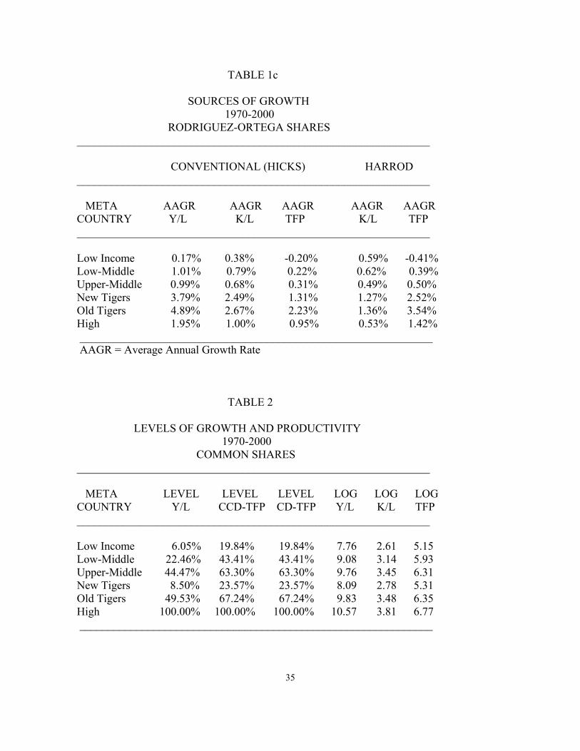
These estimates of the conventional Solow residual are shown in Tables 1a, 1b, and1c,

respectively. The first column of Table 1a, which uses the two thirds/one third share rule as the

basis for comparison, indicates that output per worker grew strongly over the period 1970 to

2000 in the High Income countries, but was close to zero in the Low Income group. The Lower

Middle and Upper Middle Income meta countries display a positive growth experience, but still

15 By contrast, Duffy and Papageorgiou (2000) find that the elasticity of substitution – and hence the labor share – falls as income increases. A recent paper by Goldar (2004) seems to lend support to their finding, as it reports a falling share over time in Indian manufacturing industry, and a low terminal value of just below 0.3 (a value consistent with the national income approach).

18

lag the growth rate of the High Income leader. The Old and New Tigers, on the other hand,

outperformed the leader in terms of growth. However, it is also the case that they started from a

lower level of output per worker.

The second and third columns of Table 1a show the sources-of-growth decomposition of

the growth rate of output per worker into its capital-deepening and TFP components. It is

apparent that capital deepening is the predominant source of growth in the Low, Lower Middle,

and Upper Middle Income countries, and that it accounts for about half of the growth in output

per worker in the High Income. The Tiger countries are the exception to this pattern with TFP as

the main source of growth, but not by a very large margin. These estimate speak directly to the

question posed in Figure 1 about the relative magnitudes of the growth rates associated with the

effects (a to b) and (b to c): capital deepening, not TFP, is the dominant effect in the poorer low-

growth countries, but this changes as the growth rate of output per worker rises. These results

also speak to the debate whether capital deepening or productivity change is the main driver of

growth (the ‘perspiration versus inspiration’ issue, as Krugman (1994) puts it). The estimates of

Table 1a suggest that both perspiration and inspiration have important roles in a successful

program of economic development. The finding that TFP grew rapidly in the (Old) Tigers stands

in stark contrast to Young (1992, 1995), who argued that the contribution of TFP was only a

negligible part of the East Asian miracle, and is more in line with Hsieh (2002).

However, there is an important caveat. A comparison of the Low Income and High

Income cases indicates that nearly sixty percent of the cross-sectional difference in the growth

rate of yt between the high income meta country and the others is due to differences in TFP

growth rates. In other words, capital deepening is the dominant source of growth over time in all

but the most rapidly growing countries, but TFP is a more important factor in explaining cross-

19

sectional differences in growth performance. These results are very consistent with the estimates

of Bosworth and Collins (2003), who use a similar set of assumptions and methods.

The results shown in Table 1b replay Table 1a using the average measured share of labor

income, β, as estimated from the data (see Table 6). Since the share in the sources-of-growth

model is a surrogate for the associated output elasticity, the shift to the measured β greatly

decreases the output elasticity of labor and increases that of capital, thereby giving greater

weight to the growth rate of kt and strengthening the capital-deepening effect. In the case of

Low Income countries, for example, the increase in the capital elasticity is from 0.33 to 0.71, and

the effect of this change is evident in the second and third columns of Table 1b. Capital

deepening is now the overwhelmingly dominant source of growth over time in all the meta

countries, although TFP is a still an important factor in explaining cross-sectional differences in

growth performance, with the exception of the most rapidly growing countries.

The estimates of Table 1c offer a view of the sources of growth that is intermediate

between the fixed 1/3-2/3 shares of Table 1a and the average measured labor shares of Table 1b.

The shares in this case are based on the Rodriguez and Ortega (2006) finding that capital’s

income share in manufacturing industry declines by 6.25 percentage points for each log-point

increase in GDP per capita. We apply this factor to the base value of capital’s share in the High

Income meta country, which we take to be 0.33. Because the Rodriguez-Ortega adjustment

generally increases capital’s weight, capital deepening is now the leading source of growth in

every meta country. However, estimates are much closer to those of Table 1a than 1b, and a

major change occurs only in the New Tiger countries.

These three tables are based on estimates of capital stock derived using PPP price

deflators. However, Bosworth and Collins (2003) warn of the sensitivity of the results to the

20

choice of price deflator. The use of national price deflators does give a somewhat different view

of the problem, and this should be borne in mind when interpreting the results. This is one more

data issue to which more attention needs to be paid. 16

C. The Sources of Development Estimates

Tables 1a, 1b, and 1c approach the analysis of growth by examining the rate of growth of

yt and the fraction explained by capital deepening and TFP. The sources-of-development

analysis examines the parallel issue about the corresponding levels: what fraction of the level of

yt is explained by the level of the capital-deepening effect and the TFP effects, that is, what is the

actual magnitude of the distances (a to b) and (b to c) in Figure 1, and how much of the overall

gap (a to c) do they explain?

Table 2 presents “level” results that differ from the preceding analysis based on growth

rates. The first column of this table, which uses the 1/3-2/3 income share convention, reports the

level of output per worker in the first five meta countries relative to the level of the High Income

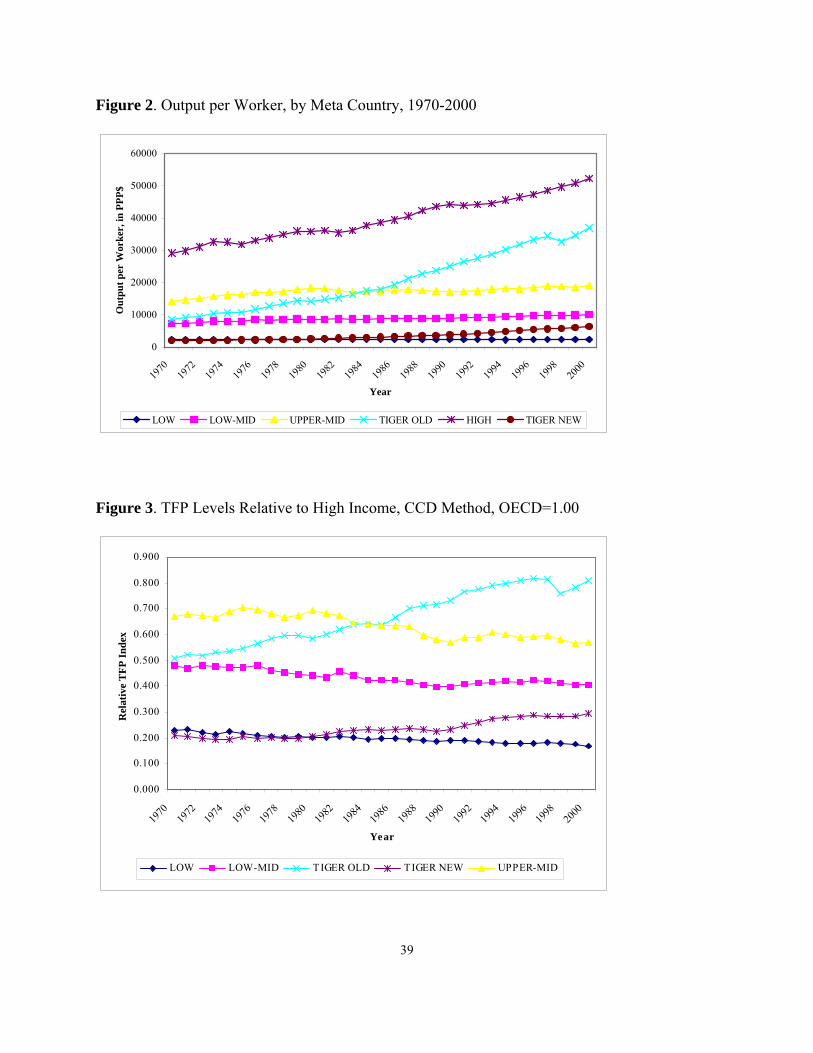
countries, and portrays the same large gap between rich and poor countries seen in Figure 2

(which plots the paths of yt over time for the four largest groups of countries and the Tigers). The

second column of Table 2 shows the relative levels of TFP, based on Caves, Christensen, and

Diewert (1982a). It is clear from this table that the level of TFP in the first five meta countries is 16 Bosworth and Collins (2003) argue that capital goods valued in national prices are a better reflection of the capital costs faced by each country. They show that PPP-based capital stocks estimates have higher growth rates than the corresponding estimates using national prices, and that the former thus lead to an understatement of the TFP performance of poor countries. Our estimates based on national prices obtained from World Development Indicators (World Bank, 2004), for the 83 (out of 112) are shown in Table A2 of the Appendix, for our six meta countries. While Table A2 generally supports the findings of Bosworth and Collins, the differences are not large enough to alter the results based on the more widely accepted PPP approach. The main difference arises in the Low Income meta country, where TFP growth does come to dominate. However, all of the growth rates for this case are quite close to zero. We have therefore opted to use the conventional PPP approach in this paper, but note that this is yet another area where data issues are important.

21

significantly below that of the High Income countries, and, while similar in pattern, are

somewhat more compressed than the relative levels of output per worker. The latter is 16 times

greater in the High Income countries compared to the Low, while the gap in productive

efficiency is ‘only’ a factor of 5. Figure 2 displays the time series trends that correspond to

column 2. It reveals the same general magnitude as the relative TFP estimates of Table 2, and

also indicates that the gap has widened over time for the Low, Lower Middle, and Upper Middle

countries, but that the Tiger countries (Old and New) are narrowing the gap in the relative TFP

level.

The last three columns of Table 2 decompose the level of output per worker into its

capital-deepening and TFP components. Following Easterly and Levine (2001), we assume that

the production function has the simple constant-returns Cobb-Douglas form yt = Atkt(1-β). The

variable At is the basis for growth of TFP in the Solow model, and the level of TFP can be

estimated by computing the ratio yt/kt(1-β). This ‘CD’ index is not necessarily equivalent to the

CCD index, but when the β shares have the same value for each country, and the Cobb-Douglas

index is normalized to the High Income countries, it gives the same values as the CCD index

(thus, the numbers in columns 2 and 3 are identical).

To assess the relative importance of capital deepening and TFP on the level of

(unnormalized) output per worker, the logarithm yt is divided between the logarithms of At and

k t(1-β). This decomposition is shown in the last three columns of Table 2, where it is apparent

that the TFP is the predominant factor explaining the level of output per worker. Moreover, a

little more than half of the cross-sectional variation among countries is explained by the

difference in the level of TFP. This is the disconnect between the growth-rate analysis of Table

1a and the level analysis of Table 2 noted above. For example, TFP growth explains none of the

22

growth rate in output per worker in the Low Income meta country, but the corresponding TFP

level explains 66% of the level of output per worker. For the Lower and Upper Middle meta

countries, these numbers are 40% and 65%, and for the High Income case, they are 49% and

64%. This disconnect is diminished, but not absent, in the high growth Tiger meta countries.

In other words, Table 1a suggests that their growth is propelled more by capital

deepening rather than TFP growth, but Table 2 indicates that the main factor in explaining the

large gap in output per worker is the persistently low levels of TFP in these countries (compare,

also, Figures 2 and 3). Not all of the 67 countries in the Low, Lower Middle, and Upper Middle

income meta groups are subject to this pattern. And, significantly, the Tiger countries display a

convergence toward the High Income case, in both output per worker and in TFP levels, powered

in part by a rapid rate of TFP growth. This pattern suggests that, in the large, successful

development programs are powered by an acceleration in TFP growth relative to that of the High

Income leaders, and that the gap in TFP levels in thereby narrowed. An acceleration in capital

per worker is also an important (albeit lesser) factor. Whether the former drives the latter, as in

the Harrodian view, or vice versa, as in the endogenous growth view, cannot be learned from

sources-of-growth estimates, but whatever the dynamics associated with TFP growth and levels,

the estimates of Tables 1a and 2 assign a centrally important role to measured TFP.

D. Empirical Results from the Harrodian and Endogenous Technology Approaches

The Harrodian version of the growth decomposition is shown in the last two columns of

Tables 1a-1c. In practical terms, Harrodian TFP in column 5 is computed by dividing the

corresponding Hicksian estimate in column 3 by labor’s income share. This procedure results in

a larger effect attributed to productivity, since part of the growth kt (the induced accumulation) is

reassigned to TFP. This result carries over from growth rates to levels, which are not shown,

23

since in the common-share Cobb-Douglas case, the Harrodian levels are a simple power

transformation (based on $) of the Hicksian level estimates of Table 2.

Endogenous growth theory implies a very different sources-of-growth decomposition.

Where the Harrodian approach reallocates the induced-accumulation part of capital formation to

TFP growth, the endogenous growth view reallocates the capital-induced part of TFP growth to

capital formation. In the most extreme form, all of TFP growth is endogenous. If additional

(endogenous growth) columns were added to Tables 1a, 1b, and 1c, with the capital-deepening

effect shown in a sixth column and the TFP effect in a seventh, the new column 6 would equal

the entire growth rate of output per worker, and the column 7 would contain nothing but zeroes.

Since this decomposition is essentially trivial, from an expositional standpoint, it is not included

in the various tables.

IV. The Predictions of Growth Theory

The insights offered in the preceding sections about the growth process and the income

gap are inherently retrospective. They are based on the experience of past decades, but do not

answer to the following question: if past trends persist into the future, will they be enough to lift

a poor nation out of poverty? Are the trends in TFP and capital formation such that the poorest

countries will ultimately converge to the levels achieved by the rich and thereby extinguish the

income gap? These questions are inherently about future outcomes, and the answers require a

fully-specified model of growth that takes into account the full range of factors that determine

the future growth path.

A. Decompositions Based on Growth Models

We have already encountered the two main contenders for this role: the endogenous

growth model and the neoclassical model of steady-state growth. The growth dynamics of the

24

former stress the role the capital formation and, in its AK form, predicts that those countries that

are able to build an initial lead in capital per worker will be able to exploit the advantage and pull

away from the others. This prediction accords well with the pattern seen in Figure 2, and implies

a fairly bleak outlook for the growth of the lower income countries. However, it does not fit well

with the experience of ‘transition’ economies like the Tigers that are able to accelerate growth by

a combination of increased capital formation and more importantly, according to Table 1a, by

even stronger TFP growth.

The neoclassical model, as interpreted by MRW (1992), does allow for some countries to

catch up to the leaders while others stagnate. MRW solve for the reduced form of the Solow

steady-state model when the technology of every country has the same Cobb-Douglas form and

output elasticities. They use the equation for steady-state output per worker, adjusted to allow

convergence to steady-state, to estimate the elasticities. In this paper, we take this equation to

estimate steady-state output per worker for each meta country, y*, by using the ‘two-thirds/one-

third’ rule for the income share as an estimate of the Cobb-Douglas elasticities, and by

estimating the other variables in the reduced form: the investment rate, σ, the rate labor force

growth, η, the rate of depreciation, δ, the Harrodian rate of technical change, λ, and the level of

TFP in the comparison year 2000, A2000.

The MRW model assumes the Cobb-Douglas form with constant returns to scale, so that

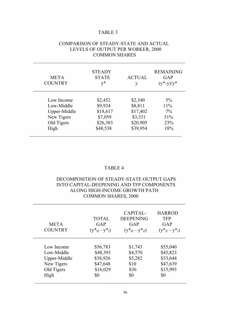
y*t = Atk*t(1-β). The steady-state solution for y* in each of the six meta countries is shown in the

first column of Table 3 for the last year in our sample, 2000. The actual level of output per

worker in 2000 is shown for comparison in the adjacent column. The salient result is that there

is a huge gap in output per worker between the Low and High Income countries (a ratio of 17 to1

in 2000), and this gap is set to persist into the indefinite future. Moreover, this is true even if the

25

Low Income meta country’s rate of productivity growth λ were to improve to the rate prevailing

in the High Income case. In fact, the Low Income country would have to improve the growth rate

of TFP to that of the High Income country just to maintain the year 2000 gap. If the λ’s shown

in last column of Table 1a persist into the future, the gap will widen. Similar remarks apply, to a

lesser extent, for the Lower Middle and Upper Middle Income meta countries. The steady-state

picture is only bright for the Old Tiger countries, whose y*2000 is around one half of the High

Income amount, and whose λ is larger.

The sources of the gap are examined in Table 4, which decomposes the gap between

steady-state output per worker in the rich and poor countries into the separate contributions of

capital-deepening and TFP. This analysis is parallel to the sources-of-development level

decomposition shown in Table 2, but the novelty here is that the decomposition refers to the

long-run equilibrium contributions of the two sources when capital formation is endogenous

(relative to a given rate of saving).

The sources of the income gap are further examined in Table 4. The difference in the

level of steady-state output per worker is in the High Income meta country (H) compared to the

Low Income (L) country is (y*H - y*L), which can be decomposed into two effects. The first is

the gap (yf - y*L), the distance between L’s steady-state y*L and the point yf. on its own

production function that it would attain if it operated with the saving and population growth

parameters of economy H rather than its own parameters. The second component of the

decomposition is the distance between the two production functions, (y*H - yf ), as measured in

the Harrodian way along the high income growth path. The two terms decompose the steady-

state output per worker gap into capital-deepening and efficiency effects based on the saving and

population growth parameters of the high income country.

26

A look at column 1 of Table 4 shows the dollar magnitude of the total gap (y*H - y*L) for

each of the meta countries in the year 2000, while the next columns gives capital-deepening, the

difference (yf - y*L), and technology effects, (y*H - yf). Several conclusions emerge from these

estimates. First, the large gap between the High Income countries and the others evident in

Figure 2 appears to be a long-run situation as long as the basic parameters of growth remain

unchanged (the exception here, as before, is the Tiger countries). Second, the gap in output per

worker is largely explained by the technology gap, not differences in the propensity to

accumulate capital relative to the growing labor force (this is also apparent in the first two

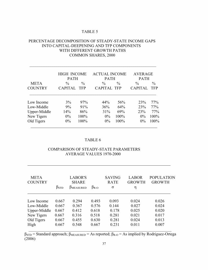
columns of Table 5, which express the Table 4 decomposition in percentage terms). Finally, the

forward-looking role played by TFP is even stronger than the role suggested by Figure 3.

However, this result must be qualified by the fact that the decomposition is not unique.

We could equally decompose the steady-state output per worker gap into capital-deepening and

efficiency effects based on the saving and population growth parameters of the low income

country. The third and fourth columns of Table 5 show the splits for these alternative paths (the

‘Actual Income Path” for each country). The alternative results are quite different, suggesting a

high degree of path dependence, and to arrive at a single index, the average values for the two

cases are shown in the last two columns of the table. The results support the overall conclusion

that the TFP effect is still the most important source for explaining the gap (y*H - y*L), as well as

the conclusion that the gap looks set to persist into the future.

B. Steady-State Sources-of-Growth Rate Estimates

Tables 4 and 5 decompose the steady-state levels of output per worker into its long-run

capital and Harrodian TFP components. For the sake of completeness, we now return to Table

1a and add the sources-of-growth rates decomposition implied by the steady-state framework.

27

The steady-state analogue to Table 1a can be calculated from the basic parameters and estimates

of the steady-state growth, since, along the steady-state path, output per worker, y*, and capital

per worker, k*, grow at the same rate λ. In other words, Harrodian productivity is the sole

driver of the steady-state growth in output per worker in the neoclassical model. Thus, the first

column of a steady-state analogue to Table 1a would record the λ appropriate for each country,

and Harrodian decomposition in the fourth and fifth columns would have the values 0 (for the

capital-deepening effect) and λ (for the TFP effect), since all capital formation is induced

accumulation and is assigned to TFP. This represents the true picture of growth, conditional on

accepting the validity of the experiment with the neoclassical model.

In the steady-state version of the standard sources-of-growth model developed by Solow,

the growth rate of output per worker is y* and the capital-deepening effect is (1- β) k*, and the

TFP effect is the residual y* - (1- β) k*. This implies that the Hicksian decomposition would

record (1- β)λ for the capital effect and βλ for the TFP contribution in an analogue to Table 1.

However, these are not the correct numbers with which to assess the relative contribution of each

effect, and this establishes the fact that the Solow residual growth model, so widely used in

empirical growth theory, is asymptotically biased. Again, this bias is the counterpart of the

simultaneous equations bias arising is econometrics from the endogeneity of capital.

V. Conclusion

Our analysis points to the persistently low levels of technological efficiency as the

proximate source of the gap between the rich and poorer countries. In this, we confirm many

other studies of this issue. We have not attempted to explain the causes of the technology gap,

be they due to institutional and environmental factors, the externalities associated with capital

formation, or whatever. We have chosen, instead, to examine the prior issue of how to measure

28

the gap, and have compared different techniques and assumptions using a common set of data.

This examination has led us to the following conclusions.

First, the conventional analysis of differential growth rates needs to be supplemented by a

parallel analysis of productivity levels. Capital deepening explains more than half of the growth

rate of output per worker in a majority of countries, while TFP explains more than half of the

corresponding gap. Only in the rapid-growth Tiger countries does TFP growth outweigh capital

formation, and then only by a small margin.

Second, the Hicks and Harrod ways of measuring the relative levels of the technology

gap are both relevant, but they are relevant for answering different questions. The former

measures the extra output that could be obtained from the current quantities of capital and labor

by moving to a higher level of TFP, while the latter includes the additional output arising from

the savings generated by the gain in productive efficiency. The latter is larger and is relevant for

understanding the overall impact of TFP, but if the goal is to understand the causes of a low level

of productive efficiency, per se, the Hicksian approach seems better suited to the task.

Third, in the endogenous growth approach, the induced-technology effect appears as a

shift in the production function in the conventional Hicks-Solow measurement framework, so a

positive gap in measured TFP is not inconsistent with the endogenous growth model. Indeed,

endogenous growth effects are among the factors than can be adduced to explain the gap.

Fourth, the measurement procedures used in the literature to measure the income and

technology gaps are inherently backward looking. A large income gap between rich and poor

countries is less of a concern if the growth paths of the two will converge in the future. This can

only be learned from a modeling exercise that endogenizes the growth path, rather than taking

the sources of growth as being exogenously determined as in the Solow residual model. We use

29

the neoclassical model for this purpose, and develop a steady-state decomposition of output per

worker into capital deepening and Harrodian-TFP components. We find that this forward-

looking model predicts that the large gap will not close in the future for most of the developing

countries unless they are able to significantly improve both the growth rates of the capital per

worker and TFP. This conclusion must be tempered by the highly abstract nature of the

neoclassical growth model, but the size of the predicted long-run gaps are suggestive of the

potential magnitude of future income gaps. The steady-state analysis is also useful in pointing

out the existence of an asymptotic bias in the conventional Solow approach to the sources of

growth.

Finally, it is important to emphasize, once again, that there are significant gaps in the

data. The problem is most apparent in the implausibly low labor shares implied by national

accounting data for lower income countries, and the resulting practice of imposing a common

two-thirds share on all countries. The output elasticities of capital and labor, as proxied by the

share, are a key determinant of output growth, and the consequences of using different measures

of the labor share are evident in the estimates of Tables 1a, 1b, and 1c of this paper. It is

intellectually disturbing that our understanding of the growth process should rest on such shaky

data foundations. And, data issues are by no means limited to the problem with measured

income shares. The accuracy of capital measures is also an issue, particularly with the

Bosworth-Collins point about the large difference that arises when national prices are substitutes

for PPP price. It would be well, in closing, to recall the words of Zvi Griliches, who observed:

“We [economists] ourselves do not put enough emphasis on the value of data and data collection in our training of graduate students and in the reward structure of our profession. It is the preparation skill of the chef that catches the professional eye, not the quality of the materials in the meal, or the effort that went into procuring them.” (AER 1994)

30

References Abramovitz, Moses, "Resource and Output Trends in the United States since 1870," American Economic Review, 46, 2, May 1956, 5-23. Barro, Robert J., “Notes on Growth Accounting,” Journal of Economic Growth, 4, June 1999, 119-137. Bentolila, Samuel, and Gilles Saint Paul, “Explaining Movements in the Labor Share,” Contributions to Macroeconomics, Berkeley Electronic Press, vol. 3, 1, 2003, 1103-1115. Bosworth, Barry P., and Susan M. Collins, "The Empirics of Growth: An Update," Brookings Papers on Economic Activity: 2, 2003, 113-206. Caves, Douglas W., Laurits R. Christensen, and W. Erwin Diewert, "Multilateral Comparisons of

Output, Input, and Productivity Using Superlative Index Numbers," Economic Journal, 92, March 1982a, 73-86.

Caves, Douglas W., Laurits R. Christensen, and W. Erwin Diewert, "The Economic Theory of Index Numbers and the Measurement of Input, Output, and Productivity," Econometrica, 50, 6, November 1982b, 1393-1414. Christensen, Laurits R., Diane Cummings, and Dale W. Jorgenson, "Relative Productivity Levels, 1947-1973: An International Comparison," European Economic Review, 16, 1981, 61-94. Denison, Edward F., Why Growth Rates Differ: Postwar Experiences in Nine Western Countries, The Brookings Institution, Washington, D.C., 1967. Diewert, W. Erwin, "Exact and Superlative Index Numbers," Journal of Econometrics, 4, 1976, 115-145. Dowrick Steven and Duc-Tho Nguyen, "OECD Comparative Economic Growth 1950-85:

Catch-up and Convergence," American Economic Review, 79(5), December 1989, 1010-1030.

Duffy, John and Chris Papageorgiou, "A Cross-Country Empirical Investigation of the

Aggregate Production Function Specification,” Journal of Economic Growth, 5(1), 87-120, March 2000.

Easterly, William and Ross Levine, "It's Not Factor Accumulation: Stylized Facts and Growth

Models," World Bank Economic Review, 15, 2, 2001. Fisher, Franklin, "Embodied Technical Change and the Existence of an Aggregate Capital

Stock," Review of Economic Studies, 1965, 326-388.

31

Fisher, Franklin, “The Existence of Aggregate Production Functions.” The Irving Fisher Lecture at the Econometric Society Meetings, Amsterdam, September 1968; Econometrica, Vol. 37, No. 4, October 1969, pp. 553–577. Färe, Rolf, Shawna Grosskopf, Mary Norris, and Zhongyang Zhang, "Productivity Growth,

Technical Progress, and Efficiency Change in Industrialized Countries," American Economic Review, 84, 1, March 1994, 66-83.

Goldar, Bishwanath, “Productivity Trends in Indian Manufacturing in the Pre- and Post-Reform

Periods,” Working Paper No. 137, Indian Council for Research on International Economic Relations, New Delhi, India.

Gollin, Douglas, “Getting Income Shares Right,” Journal of Political Economy, 110(2), 2002, 458-74. Griliches , Zvi, "Productivity, R&D, and the Data Constraint," American Economic Review, 84,

1, March 1994, 1-23. Hall, Robert E. and Charles I. Jones, “Why Do Some Countries Produce So Much More Output Per Worker Than Others?” The Quarterly Journal of Economics 114(1), 1999, 83- 116. Harrison, Ann E., “Has Globalization Eroded Labor’s Share? Some Cross-Country Evidence,” University of California, Berkeley, working paper, October 2002. Heston, Alan, Robert Summers and Bettina Aten, Penn World Table Version 6.1, Center for

International Comparisons at the University of Pennsylvania (CICUP), October 2002. Hsieh, Chang-Tai, “What Explains the Industrial Revolution in East Asia? Evidence from the

Factor Markets, American Economic Review, 92, 3, June 2002, 502-26. Hulten, Charles R., “Divisia Index Numbers,” Econometrica, 41, 6, November 1973, 1017-25. Hulten, Charles R., "Technical Change and the Reproducibility of Capital," American Economic Review, 65, 5, December 1975, 956-965. Hulten, Charles R., "On the 'Importance' of Productivity Change," American Economic Review, 69, 1979, 126-136. Hulten, Charles R., "Total Factor Productivity: A Short Biography," in New Developments in Productivity Analysis, Charles R. Hulten, Edwin R. Dean, and Michael J. Harper, eds., Studies in Income and Wealth, vol. 63, The University of Chicago Press for the National Bureau of Economic Research, Chicago, 2001, 1-47.

32

Hulten, and Charles R. and Mieko Nishimizu, "The Importance of Productivity Change in the Economic Growth of Nine Industrialized Countries," in Lagging Productivity Growth: Causes and Remedies, Shlomo Maital and Noah M. Meltz, eds., Ballinger, Cambridge, Mass., 1980, 85-100. Isaksson, Anders, “World Productivity Database: A Technical Description”, Vienna: UNIDO.

January 2007. Jorgenson, Dale W. and Zvi Griliches, "The Explanation of Productivity Change," Review of Economic Studies, 34, July 1967, 349-83. Jorgenson, Dale W. and Mieko Nishimizu, “U.S. and Japanese Economic Growth, 1952-1974. An International Comparison.” Economic Journal, December, 1978, 707-726. Klenow, Peter, and Andrés Rodriguez-Clare, “The Neoclassical Revival in Growth Economics: Has It Gone Too Far?” In National Bureau of Economic Research Macroeconomics Annual 1997, edited by Ben S. Bernanke and Julio Rotemberg, Cambridge, MA: MIT Press, 1997, 73-103. Krugman, Paul, "The Myth of Asia's Miracle," Foreign Affairs, 73, 6, November/December, 1994, 62-77. Landes, David S., The Wealth and Poverty of Nations: Why Some Countries are So Rich and Some So Poor, W.W. Norton & Company, New York, 1998. Lucas, Robert E. Jr., “On the Mechanics of Economic Development,” Journal of Monetary Economics, 22, 1988, 3-42. Maddison, Angus, "Growth and Slowdown in Advanced Capitalist Economies: Techniques and Quantitative Assessment," Journal of Economic Literature, 25, 2, June 1987, 649-698. Mankiw, N. Gregory, David Romer, and David N. Weil, "Contribution to the Empirics of Economic Growth, Harvard University," The Quarterly Journal of Economics, May 1992, 407-437. Nishimizu, Mieko and Charles Hulten, “The Sources of Japanese Economic Growth, 1955-71,” Review of Economics and Statistics, 60(3), 1978, 351-361. Rodriguez, Francisco and Daniel Ortega, “Are Capital Shares Higher in Poor Countries?

Evidence from Industrial Surveys,” Wesleyan Economics Working Papers, No: 2006-023, 2006.

33

Romer, Paul M., “Increasing Returns and Long-Run Growth,” Journal of Political Economy, 94(5), 1986, 1002-1052. Rymes, Thomas K., On Concepts of Capital and Technical Change, Cambridge Mass., Cambridge University Press, 1971. Solow, Robert M., “A Contribution to the Theory of Economic Growth,” Quarterly Journal of Economics, 70, 1956, February, 65-94. Solow, Robert M., “Technical Change and the Aggregate Production Function,” Review of Economics and Statistics, 39, 1957, 312-320. Solow, Robert M., “Some Recent Developments in the Theory of Production,” in The Theory and Empirical Analysis of Production, Murray Brown, ed., Studies in Income and Wealth, vol. 31, The Columbia University Press for the National Bureau of Economic Research, New York and London, 1967, 25-50. United Nations, National Accounts Statistics: Main Aggregates and Detailed Tables, Department

of Economic and Social Affairs, Statistics Division, United Nations, New York, various years.

Young, Alwyn, "A Tale of Two Cities: Factor Accumulation and Technical Change in Hong Kong and Singapore, In Blanchard, O.J., and S. Fisher, eds., NBER Macroeconomics Annual 1992, Cambridge Mass: MIT Press, 1992, 13-54. Young, Alwyn, “Tyranny of Numbers: Confronting the Statistical Realities of the East Asian Growth Experience,” Quarterly Journal of Economics, August 1995, 641-680.

World Bank, World Development Indicators 2004, World Bank, Washington, DC, 2004.

34

TABLE 1a SOURCES OF GROWTH COMMON SHARES 1970-2000 _________________________________________________________________ CONVENTIONAL (HICKS) HARROD _________________________________________________________________ META AAGR AAGR AAGR AAGR AAGR COUNTRY Y/L K/L TFP K/L TFP __________________________________________________________________ Low Income 0.17% 0.25% -0.07% 0.28% -0.11% Low-Middle 1.01% 0.61% 0.40% 0.41% 0.60% Upper-Middle 0.99% 0.59% 0.40% 0.39% 0.60% New Tigers 3.79% 1.70% 2.09% 0.68% 3.12% Old Tigers 4.89% 2.37% 2.52% 1.13% 3.76% High 1.95% 1.00% 0.95% 0.53% 1.42% _________________________________________________________________ AAGR = Average Annual Growth Rate TABLE 1 b SOURCES OF GROWTH 1970-2000 MEASURED SHARES ______________________________________________________________ CONVENTIONAL (HICKS) HARROD ______________________________________________________________ META AAGR AAGR AAGR AAGR AAGR COUNTRY Y/L K/L TFP K/L TFP ______________________________________________________________ Low Income 0.17% 0.52% -0.35% 1.37% -1.19% Low-Middle 1.01% 1.17% -0.16% 1.45% -0.44% Upper-Middle 0.99% 1.05% -0.06% 1.14% -0.15% New Tigers 3.79% 3.53% 0.26% 2.97% 0.83% Old Tigers 4.89% 3.92% 0.97% 2.76% 2.13% High 1.95% 1.36% 0.58% 0.88% 1.07% ______________________________________________________________ AAGR = Average Annual Growth Rate

35

TABLE 1c SOURCES OF GROWTH 1970-2000 RODRIGUEZ-ORTEGA SHARES ______________________________________________________________ CONVENTIONAL (HICKS) HARROD ______________________________________________________________ META AAGR AAGR AAGR AAGR AAGR COUNTRY Y/L K/L TFP K/L TFP ______________________________________________________________ Low Income 0.17% 0.38% -0.20% 0.59% -0.41% Low-Middle 1.01% 0.79% 0.22% 0.62% 0.39% Upper-Middle 0.99% 0.68% 0.31% 0.49% 0.50% New Tigers 3.79% 2.49% 1.31% 1.27% 2.52% Old Tigers 4.89% 2.67% 2.23% 1.36% 3.54% High 1.95% 1.00% 0.95% 0.53% 1.42% ______________________________________________________________ AAGR = Average Annual Growth Rate TABLE 2 LEVELS OF GROWTH AND PRODUCTIVITY 1970-2000 COMMON SHARES ______________________________________________________________ META LEVEL LEVEL LEVEL LOG LOG LOG COUNTRY Y/L CCD-TFP CD-TFP Y/L K/L TFP ______________________________________________________________ Low Income 6.05% 19.84% 19.84% 7.76 2.61 5.15 Low-Middle 22.46% 43.41% 43.41% 9.08 3.14 5.93 Upper-Middle 44.47% 63.30% 63.30% 9.76 3.45 6.31 New Tigers 8.50% 23.57% 23.57% 8.09 2.78 5.31 Old Tigers 49.53% 67.24% 67.24% 9.83 3.48 6.35 High 100.00% 100.00% 100.00% 10.57 3.81 6.77 ______________________________________________________________

36

TABLE 3 COMPARISON OF STEADY-STATE AND ACTUAL LEVELS OF OUTPUT PER WORKER, 2000 COMMON SHARES ______________________________________________________________ STEADY REMAINING META STATE ACTUAL GAP COUNTRY y* y (y*-y)/y* ______________________________________________________________

Low Income $2,452 $2,340 5% Low-Middle $9,924 $8,811 11%

Upper-Middle $18,617 $17,402 7% New Tigers $7,059 $3,531 51% Old Tigers $26,383 $20,905 23%

High $48,538 $39,954 18% ______________________________________________________________ TABLE 4 DECOMPOSITION OF STEADY-STATE OUTPUT GAPS INTO CAPITAL-DEEPENING AND TFP COMPONENTS ALONG HIGH-INCOME GROWTH PATH COMMON SHARES, 2000 ______________________________________________________________ CAPITAL- HARROD TOTAL DEEPENING TFP META GAP GAP GAP COUNTRY (y*H – y*i) (y*H – y*if) (y*if – y*i) ______________________________________________________________ Low Income $56,783 $1,743 $55,040 Low-Middle $48,393 $4,570 $43,823 Upper-Middle $38,926 $5,282 $33,644 New Tigers $47,648 $10 $47,639

Old Tigers $16,029 $36 $15,993 High $0 $0 $0 ______________________________________________________________

37

TABLE 5 PERCENTAGE DECOMPOSITION OF STEADY-STATE INCOME GAPS INTO CAPITAL-DEEPENING AND TFP COMPONENTS WITH DIFFERENT GROWTH PATHS COMMON SHARES, 2000 ______________________________________________________________ HIGH INCOME ACTUAL INCOME AVERAGE PATH PATH PATH META % % % % % % COUNTRY CAPITAL TFP CAPITAL TFP CAPITAL TFP ______________________________________________________________ Low Income 3% 97% 44% 56% 23% 77% Low-Middle 9% 91% 36% 64% 23% 77% Upper-Middle 14% 86% 31% 69% 23% 77% New Tigers 0% 100% 0% 100% 0% 100% Old Tigers 0% 100% 0% 100% 0% 100% ______________________________________________________________ TABLE 6 COMPARISON OF STEADY-STATE PARAMETERS AVERAGE VALUES 1970-2000 ______________________________________________________________________ META LABOR'S SAVING LABOR POPULATION COUNTRY SHARE RATE GROWTH GROWTH βSTD βMEASURED βR-O σ η ______________________________________________________________________ Low Income 0.667 0.294 0.493 0.093 0.024 0.026 Low-Middle 0.667 0.367 0.576 0.144 0.027 0.024 Upper-Middle 0.667 0.412 0.618 0.178 0.025 0.020 New Tigers 0.667 0.316 0.518 0.281 0.021 0.017 Old Tigers 0.667 0.455 0.630 0.281 0.024 0.013 High 0.667 0.548 0.667 0.231 0.011 0.007 ______________________________________________________________________ βSTD = Standard approach; βMEASURED = As reported; βR-O = As implied by Rodriguez-Ortega (2006)

38

Figure 1. Output per Worker, Level of TFP and Capital-deepening effect

OUTPUT/LABOR (y)

CAPITAL/LABOR (k)

y00

kk

y70

00

ab

c y = A f(k)00

y = A f(k)70

d

70

y'00

P

e

39

Figure 2. Output per Worker, by Meta Country, 1970-2000

Figure 3. TFP Levels Relative to High Income, CCD Method, OECD=1.00

0

10000

20000

30000

40000

50000

60000

1970

1972

1974

1976

1978

1980

1982

1984

1986

1988

1990

1992

1994

1996

1998

2000

Year

Out

put p

er W

orke

r, in

PPP

$

LOW LOW-MID UPPER-MID TIGER OLD HIGH TIGER NEW

0.000

0.100

0.200

0.300

0.400

0.500

0.600

0.700

0.800

0.900

1970

1972

1974

1976

1978

1980

1982

1984

1986

1988

1990

1992

1994

1996

1998

2000

Year

Rel

ativ

e T

FP In

dex

LOW LOW-MID TIGER OLD TIGER NEW UPPER-MID

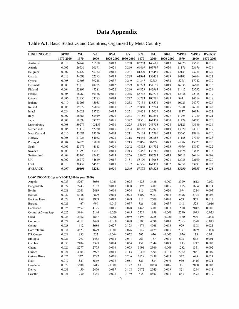
40

Data Appendix Table A.1. Basic Statistics and Countries, Organized by Meta Country HIGH INCOME DPOP Y/L Y/L DY/L I/Y K/L K/L DK/L Y/POP Y/POP DY/POP 1970-2000 1970 2000 1970-2000 1970-2000 1970 2000 1970-2000 1970 2000 1970-2000Australia 0.013 34747 51568 0.013 0.238 86703 148660 0.017 14820 25559 0.018 Austria 0.003 26736 50591 0.021 0.260 66469 169797 0.030 11176 23676 0.024 Belgium 0.002 32427 56752 0.018 0.231 81200 176457 0.025 12143 23781 0.022 Canada 0.012 34692 52295 0.013 0.228 61994 152421 0.029 14102 26904 0.021 Cyprus 0.008 12603 39218 0.037 0.249 34347 92786 0.032 5275 17742 0.039 Denmark 0.003 33218 48255 0.012 0.229 83723 151198 0.019 16038 26608 0.016 Finland 0.004 23899 47281 0.022 0.260 64823 145963 0.026 11412 23792 0.024 France 0.005 28960 49136 0.017 0.246 65718 160775 0.029 12336 22358 0.019 Greece 0.006 21755 33783 0.014 0.247 50713 103785 0.023 8441 14614 0.018 Iceland 0.010 25205 45055 0.019 0.258 77138 138571 0.019 10925 24777 0.026 Ireland 0.008 19079 65054 0.040 0.192 28880 115744 0.045 7260 26381 0.042 Israel 0.024 24021 38762 0.015 0.271 54458 113059 0.024 8837 16954 0.021 Italy 0.002 28883 53949 0.020 0.233 74156 169291 0.027 11294 21780 0.021 Japan 0.007 18098 38737 0.025 0.322 34551 161357 0.050 11474 24675 0.025 Luxembourg 0.008 39277 103133 0.031 0.225 115514 243753 0.024 15121 43989 0.034 Netherlands 0.006 33112 52230 0.015 0.234 84187 152928 0.019 13320 24313 0.019 New Zealand 0.010 35083 39360 0.004 0.211 78165 115780 0.013 13665 18816 0.010 Norway 0.005 27024 54032 0.022 0.318 91446 200385 0.025 11188 27060 0.028 Portugal 0.004 14823 35008 0.028 0.213 25056 96372 0.043 6296 15923 0.030 Spain 0.005 23675 44113 0.020 0.242 47853 134732 0.033 9076 18047 0.022 Sweden 0.003 31990 45453 0.011 0.213 79456 133786 0.017 14828 23635 0.015 Switzerland 0.004 43346 47412 0.003 0.266 129962 192283 0.013 20611 26414 0.008 UK 0.002 26272 44649 0.017 0.181 58109 113065 0.021 12085 22190 0.020 USA 0.010 38432 64537 0.017 0.197 60506 161391 0.032 16351 33293 0.023 AVERAGE 0.007 29108 52211 0.020 0.240 57171 154321 0.033 13290 26595 0.023 LOW INCOME (up to YPOP 3,000 in year 2000) Angola 0.023 5767 3050 -0.021 0.075 4223 3428 -0.007 3329 1612 -0.023 Bangladesh 0.022 2243 3187 0.011 0.098 3193 3707 0.005 1105 1684 0.014 Benin 0.028 2041 2489 0.006 0.074 816 2079 0.030 1094 1214 0.003 Bolivia 0.022 6036 6829 0.004 0.094 8409 9053 0.002 2498 2724 0.003 Burkina Faso 0.022 1159 1939 0.017 0.099 717 2509 0.040 669 957 0.012 Burundi 0.021 1467 990 -0.013 0.057 326 1028 0.037 848 523 -0.016 Cameroon 0.026 2552 4125 0.015 0.078 1445 3981 0.033 1580 2042 0.008 Central African Rep. 0.022 3964 2144 -0.020 0.045 2529 1959 -0.008 2240 1045 -0.025 Chad 0.024 2352 1837 -0.008 0.089 4196 2285 -0.020 1180 909 -0.008 Comoros 0.024 4811 3498 -0.010 0.078 3005 4090 0.010 2353 1578 -0.013 Congo 0.028 1612 3686 0.027 0.173 4476 4968 0.003 929 1808 0.021 Cote d'Ivoire 0.034 4823 4679 -0.001 0.076 3547 4179 0.005 2391 1869 -0.008 DR Congo 0.029 1835 252 -0.064 0.052 702 636 -0.003 1056 118 -0.071 Ethiopia 0.026 1293 1483 0.004 0.041 763 787 0.001 608 635 0.001 Gambia 0.033 2104 2393 0.004 0.064 451 2044 0.049 1113 1217 0.003 Ghana 0.026 2277 2775 0.006 0.073 3091 2360 -0.009 1282 1351 0.002 Guinea 0.021 4304 5977 0.011 0.113 10496 7794 -0.010 2282 2831 0.007 Guinea Bissau 0.027 577 1287 0.026 0.206 2628 2859 0.003 332 688 0.024 Haiti 0.017 1827 5569 0.036 0.051 523 1834 0.040 930 2416 0.031 Honduras 0.029 5608 5415 -0.001 0.127 6318 10234 0.016 1861 2050 0.003 Kenya 0.031 1450 2476 0.017 0.108 2072 2743 0.009 821 1244 0.013 Lesotho 0.021 1730 3365 0.021 0.189 536 10260 0.095 883 1592 0.019

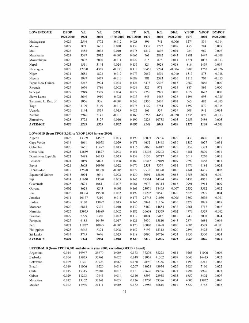
41

LOW INCOME DPOP Y/L Y/L DY/L I/Y K/L K/L DK/L Y/POP Y/POP DY/POP 1970-2000 1970 2000 1970-2000 1970-2000 1970 2000 1970-2000 1970 2000 1970-2000Madagascar 0.026 2546 1772 -0.012 0.028 896 741 -0.006 1274 836 -0.014 Malawi 0.027 871 1631 0.020 0.138 1337 1722 0.008 455 784 0.018 Mali 0.023 1485 2033 0.010 0.075 1812 1896 0.001 784 969 0.007 Mauritania 0.024 3397 2912 -0.005 0.067 761 2892 0.043 1881 1447 -0.008 Mozambique 0.020 2807 2000 -0.011 0.027 615 875 0.011 1571 1037 -0.013 Nepal 0.023 1511 3144 0.024 0.135 824 5028 0.058 816 1459 0.019 Nicaragua 0.028 12280 4367 -0.033 0.117 10451 9274 -0.004 3980 1767 -0.026 Niger 0.031 2653 1823 -0.012 0.073 2052 1501 -0.010 1519 875 -0.018 Nigeria 0.028 1997 1479 -0.010 0.089 781 2383 0.036 1113 707 -0.015 Papua New Guinea 0.023 5247 5924 0.004 0.124 6473 9592 0.013 2862 2866 0.000 Rwanda 0.027 1676 1786 0.002 0.039 325 971 0.035 887 895 0.000 Senegal 0.027 2949 3389 0.004 0.072 2758 2977 0.002 1627 1622 0.000 Sierra Leone 0.021 3649 1910 -0.021 0.033 645 1468 0.026 1496 695 -0.025 Tanzania, U. Rep. of 0.029 1056 938 -0.004 0.243 2356 2405 0.001 565 482 -0.005 Togo 0.026 3109 2149 -0.012 0.078 1129 2784 0.029 1397 870 -0.015 Uganda 0.026 1144 1835 0.015 0.023 161 537 0.039 608 941 0.014 Zambia 0.028 2946 2141 -0.010 0.169 8255 4457 -0.020 1335 892 -0.013 Zimbabwe 0.028 3723 5127 0.010 0.199 9226 10738 0.005 2155 2486 0.005 AVERAGE 0.026 2239 2359 0.002 0.095 2142 2843 0.009 1176 1138 -0.001 LOW-MID (from YPOP 3,001 to YPOP 6,000 in year 2000) Algeria 0.026 13369 14527 0.003 0.190 16093 29706 0.020 3433 4896 0.011 Cape Verde 0.016 4061 10078 0.029 0.171 4652 15448 0.039 1387 4027 0.034 Colombia 0.020 7651 11477 0.013 0.116 7860 16847 0.025 3159 5383 0.017 Costa Rica 0.025 13639 14827 0.003 0.151 13398 26203 0.022 4181 5870 0.011 Dominican Republic 0.021 7488 16173 0.025 0.138 6156 20717 0.039 2018 5270 0.031 Ecuador 0.024 7069 9023 0.008 0.189 16442 22049 0.009 2292 3468 0.013 Egypt 0.021 5603 10970 0.022 0.076 2553 7379 0.034 1970 4184 0.024 El Salvador 0.018 12578 10368 -0.006 0.072 7532 10390 0.010 4141 4435 0.002 Equatorial Guinea 0.015 8094 8641 0.002 0.130 3091 15860 0.053 3758 3604 -0.001 Fiji 0.014 11620 13580 0.005 0.147 19314 24384 0.008 3433 4971 0.012 Guatemala 0.025 8673 10611 0.007 0.081 6972 10314 0.013 2991 3914 0.009 Guyana 0.002 8628 8243 -0.001 0.163 23071 18465 -0.007 2432 3532 0.012 Iran 0.026 18304 19560 0.002 0.197 17202 38541 0.026 5225 5995 0.004 Jamaica 0.011 10177 7310 -0.011 0.173 24743 21030 -0.005 3867 3693 -0.001 Jordan 0.038 8120 13087 0.015 0.146 6841 21156 0.036 2228 3895 0.018 Morocco 0.020 6815 9301 0.010 0.139 5460 14654 0.032 2261 3717 0.016 Namibia 0.025 13955 14689 0.002 0.182 26608 28559 0.002 4770 4529 -0.002 Pakistan 0.027 2729 5360 0.022 0.117 4024 6412 0.015 943 2008 0.024 Paraguay 0.027 6183 10439 0.017 0.121 3930 15810 0.045 2874 4684 0.016 Peru 0.021 11927 10095 -0.005 0.170 26080 25698 0.000 4686 4589 -0.001 Philippines 0.023 6548 8374 0.008 0.152 8197 15312 0.020 2396 3425 0.012 Sri Lanka 0.014 3745 7646 0.023 0.119 2090 10726 0.053 1557 3300 0.024 AVERAGE 0.024 7374 9984 0.010 0.143 8417 15835 0.021 2560 3846 0.013 UPPER-MID (from YPOP 6,001 and above in year 2000, excluding OECD + Israel) Argentina 0.014 19967 25670 0.008 0.173 37276 58223 0.014 9265 11006 0.006 Barbados 0.004 15935 32961 0.023 0.148 31065 41302 0.009 6040 16415 0.032 Botswana 0.029 3126 23926 0.066 0.188 2896 32356 0.078 1193 8241 0.062 Brazil 0.019 11006 19220 0.018 0.207 18028 43954 0.029 3620 7190 0.022 Chile 0.015 15345 25084 0.016 0.151 25676 49286 0.021 4794 9926 0.023 Gabon 0.029 11293 17645 0.014 0.140 8597 23958 0.033 6857 8402 0.007 Mauritius 0.012 13162 32241 0.029 0.126 13700 39386 0.034 4005 13932 0.040 Mexico 0.022 17965 21111 0.005 0.182 27956 46815 0.017 5522 8762 0.015

42

UPPER-MID DPOP Y/L Y/L DY/L I/Y K/L K/L DK/L Y/POP Y/POP DY/POP 1970-2000 1970 2000 1970-2000 1970-2000 1970 2000 1970-2000 1970 2000 1970-2000Panama 0.021 11357 14382 0.008 0.207 17391 37650 0.025 3824 6066 0.015 Seychelles 0.013 8470 23552 0.033 0.149 4934 44543 0.071 4091 10241 0.030 South Africa 0.021 18415 18488 0.000 0.120 23582 25070 0.002 6878 7541 0.003 Syria 0.031 26235 28817 0.003 0.190 34728 14163 -0.029 7542 9193 0.006 Trinidad and Tobago 0.009 19842 25188 0.008 0.106 13058 33090 0.030 6582 11175 0.017 Tunisia 0.020 8573 17124 0.022 0.160 20720 26610 0.008 2568 6776 0.031 Turkey 0.020 8017 14125 0.018 0.162 8040 29528 0.042 3619 6832 0.021 Uruguay 0.006 13579 21150 0.014 0.121 19073 34882 0.019 6131 9622 0.015 Venezuela 0.026 35399 15705 -0.026 0.168 44808 36511 -0.007 10528 6420 -0.016 AVERAGE 0.020 14566 19492 0.009 0.159 22076 40132 0.019 5184 7924 0.014 OLD TIGERS Hong Kong, SAR of China 0.018 15587 51469 0.039 0.249 28329 138086 0.051 6506 26699 0.046 Korea, Republic of 0.012 7676 31239 0.045 0.311 9584 98424 0.075 2716 15876 0.057 Singapore 0.021 15085 50809 0.039 0.454 32892 187383 0.056 5279 28869 0.055 Taiwan, P. of China 0.013 7282 42402 0.057 0.194 6392 78537 0.081 2790 19034 0.062 AVERAGE 0.013 8513 36922 0.048 0.302 11132 102174 0.074 3120 18312 0.059 NEW TIGERS China 0.014 1583 6175 0.044 0.178 1564 10624 0.062 815 3747 0.049 India 0.020 2454 5587 0.027 0.118 2470 6729 0.032 1073 2479 0.027 Indonesia 0.019 2865 7677 0.032 0.146 1635 13772 0.069 1087 3642 0.039 Malaysia 0.025 8377 23994 0.034 0.223 10090 54710 0.055 2884 9919 0.040 Thailand 0.017 3758 11308 0.036 0.309 7486 36890 0.051 1822 6857 0.043 AVERAGE 0.017 2036 6355 0.037 0.195 2052 10587 0.054 966 3367 0.041 Note: The averages have been computed based on the meta-country averages. For example, output per worker in 2000 has been obtained by first summing income and workers separately for a given meta country, thereafter dividing total income with total workers and then dividing this ratio by the number of countries. An alternative way, leading to a slightly different result, is to first compute income per worker for each country, sum the country results and then divide this total by the number of countries. DPOP = Average annual growth rate (AAGR) of population; Y/L = GDP per worker; DY/L = AAGR of GDP per worker; I/Y = Investment share in GDP; K/L = capital-labor ratio; DK/L = AAGR of capital-labor ratio (i.e. capital deepening); Y/POP = GDP per capita; and DY/POP = AAGR of GDP per capita.

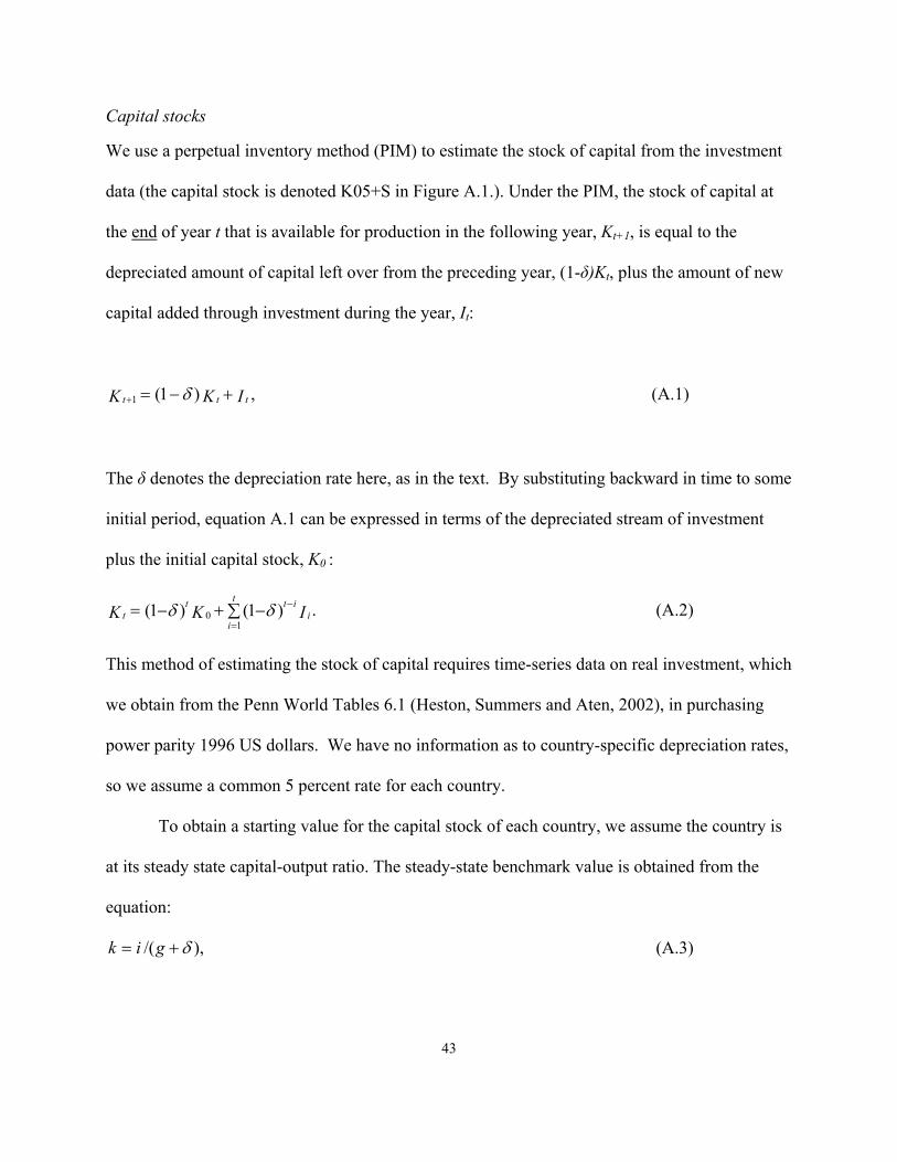
43

Capital stocks

We use a perpetual inventory method (PIM) to estimate the stock of capital from the investment

data (the capital stock is denoted K05+S in Figure A.1.). Under the PIM, the stock of capital at

the end of year t that is available for production in the following year, Kt+1, is equal to the

depreciated amount of capital left over from the preceding year, (1-δ)Kt, plus the amount of new

capital added through investment during the year, It:

,)1(1 IKK ttt +−=+ δ (A.1)

The δ denotes the depreciation rate here, as in the text. By substituting backward in time to some

initial period, equation A.1 can be expressed in terms of the depreciated stream of investment

plus the initial capital stock, K0 :

.)1()1(1

0 IKK i

t

i

ittt ∑ −+−=

=

−δδ (A.2)

This method of estimating the stock of capital requires time-series data on real investment, which

we obtain from the Penn World Tables 6.1 (Heston, Summers and Aten, 2002), in purchasing

power parity 1996 US dollars. We have no information as to country-specific depreciation rates,

so we assume a common 5 percent rate for each country.

To obtain a starting value for the capital stock of each country, we assume the country is

at its steady state capital-output ratio. The steady-state benchmark value is obtained from the

equation:

),/( δ+= gik (A.3)

44

where k = K/Y (i.e. capital-output ratio), g = the growth rate of real Y (i.e. growth of GDP), and i

= I/Y (i.e. investment rate). The steady-state growth of GDP (g) and the investment rate (i),

respectively, are calculated as the annual average over 10 years (1960-1969). Inserting these into

(A.3) gives k and the benchmark is obtained by multiplying k by initial GDP. Thereafter, we add

10 years of investment to the benchmark and this marks the initial capital stock, K0.

We have also investigated the robustness of this procedure against two other

computational methods. The first alternative is to use the steady-state approach discussed above

to compute the initial capital stock, K1970, and thereafter apply the perpetual inventory method to

the remaining years (KS). Our second procedure is to use the perpetual inventory method, but

this time without the steady-state approach to obtaining a benchmark, i.e. the benchmark is zero

in 1960. The accumulation of 10 years of investment is then taken to represent the initial capital

stock in 1970 (K05).

Figure A.1 shows how the three capital stocks actually tend to converge over time and

this leads us to have faith in our choice of calculating capital stock, implying a reasonably high

degree of robustness to our method of estimating the initial level of capital.

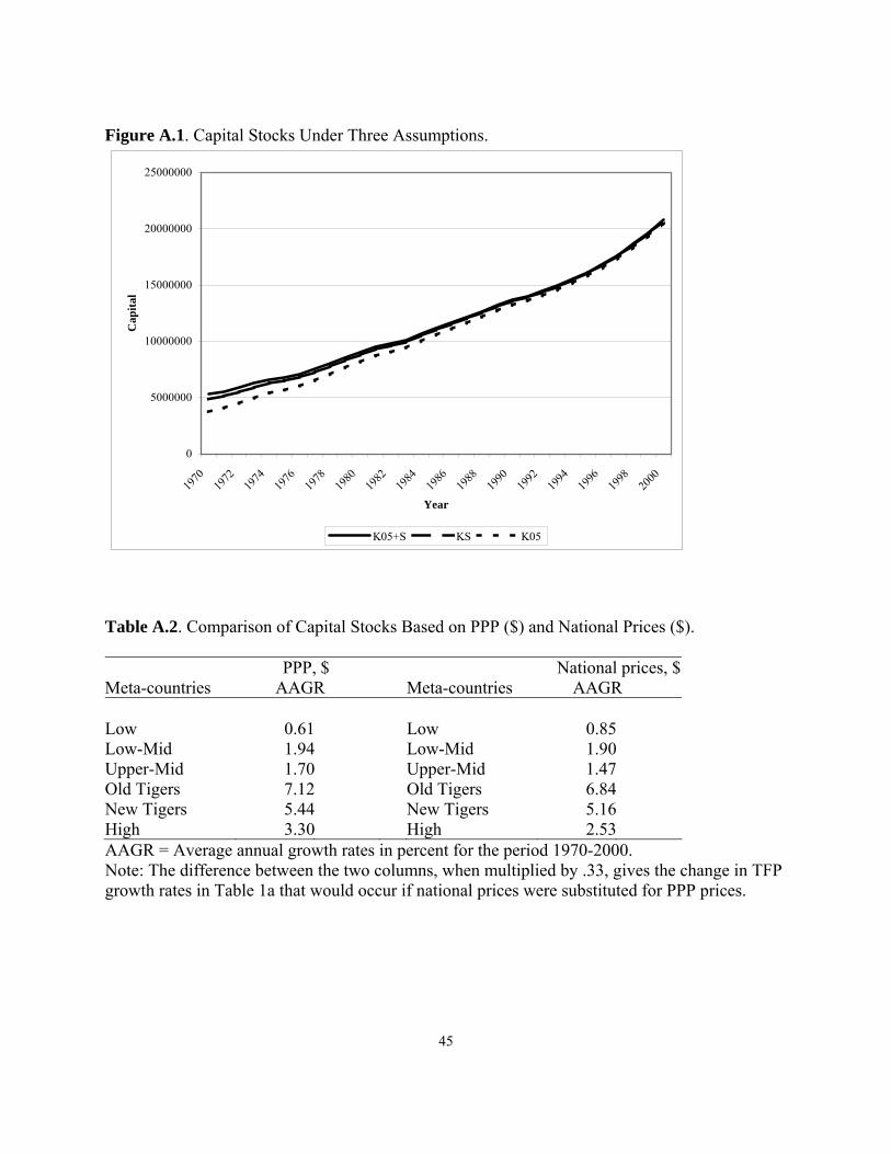
45

Figure A.1. Capital Stocks Under Three Assumptions.

Table A.2. Comparison of Capital Stocks Based on PPP ($) and National Prices ($).

PPP, $ National prices, $ Meta-countries AAGR Meta-countries AAGR Low 0.61 Low 0.85Low-Mid 1.94 Low-Mid 1.90Upper-Mid 1.70 Upper-Mid 1.47Old Tigers 7.12 Old Tigers 6.84New Tigers 5.44 New Tigers 5.16High 3.30 High 2.53AAGR = Average annual growth rates in percent for the period 1970-2000. Note: The difference between the two columns, when multiplied by .33, gives the change in TFP growth rates in Table 1a that would occur if national prices were substituted for PPP prices.

0

5000000

10000000

15000000

20000000

25000000

1970

1972

1974

1976

1978

1980

1982

1984

1986

1988

1990

1992

1994

1996

1998

2000

Year

Cap

ital

K05+S KS K05

46

Labor shares

It is standard in cross-country analysis to assume common labor shares across countries, with a

two-thirds share commonly assigned to labor (Gollin (2002)). However, the labor shares are

calculated from published data reveal very large differences across countries.17 Figure A.2

reveals just how large the differences are, and how far short of the two-thirds share the actual

estimates are. In general, labor shares increase with income level of the meta country, although

they remain fairly constant within meta countries.

Figure A.2. Labor’s Income Share for 6 Meta-Countries

17 Data on labor shares are not available for all countries. The average labor shares are therefore based on meta countries excluding the following countries: HIGH Cyprus; LOW Bangladesh, Comoros, D.R. Congo, Ethiopia, Gambia, Guinea and Nepal; LOW-MID Cape Verde, El Salvador, Equatorial Guinea, Guatemala, Pakistan and Syria; NEW TIGERS Indonesia.

0

0.1

0.2

0.3

0.4

0.5

0.6

0.7

0.8

1970

1971

1972

1973

1974

1975

1976

1977

1978

1979

1980

1981

1982

1983

1984

1985

1986

1987

1988

1989

1990

1991

1992

1993

1994

1995

1996

1997

1998

1999

2000

Year

Lab

or's

shar

e

HIGH-INC LOW LOW-MID UPP-MID OLD TIGERS NEW TIGERS STANDARD