Brigham Young UniversityBYU ScholarsArchive

All Theses and Dissertations

1965-8

The Vibration Response of Laminated OrthotropicPlatesMax E. Waddoups Jr.Brigham Young University - Provo

Follow this and additional works at: https://scholarsarchive.byu.edu/etd

Part of the Mechanical Engineering Commons

This Thesis is brought to you for free and open access by BYU ScholarsArchive. It has been accepted for inclusion in All Theses and Dissertations by anauthorized administrator of BYU ScholarsArchive. For more information, please contact scholarsarchive@byu.edu, ellen_amatangelo@byu.edu.

BYU ScholarsArchive CitationWaddoups, Max E. Jr., "The Vibration Response of Laminated Orthotropic Plates" (1965). All Theses and Dissertations. 7204.https://scholarsarchive.byu.edu/etd/7204

THE VIBRATION RESPONSE OF LAMINATED

ORTHOTROPIC PLATES

A Thesis Presented to the Faculty of

the Department of Mechanical Engineering Brigham Young University

In Partial Fulfillment

of the Requirements for the Degree Master of Science

byMax E. Waddoups, Jr.

August 1965

This thesis, by Max E. Waddoups, Jr., is accepted in its present form by the Department of Mechanical Engineering of Brigham Young University as satisfying the thesis requirements for the degree of Master of Science.

iii

ACKNOWLEDGEMENTS

I would like to express my sincere appreciation to some of the people and organizations who have made this study possible.

First, I would like to thank the Brigham Young University Research Division for the research grant which supported this study. Also, I owe a large debt of grati­tude to the management of Minnesota Mining and Manufacturing Company for the fabrication and later donation of the excellent Scotchplj^ glass reinforced plastic test specimens which were used for the experimental verification of the problem considered,

I would also like to take this opportunity to thank Assistant Professor Joseph C, Free, who originally conceived the study, gave me the opportunity to do the work and then provided advice and council throughout the the execution of the research task.

And finally, I would like to thank Mrs, Marlene Hyte for helping me prepare the manuscript and my wife, Patricia, for her unselfish devotion and support throughout my Graduate School attendance.

I would also

would like

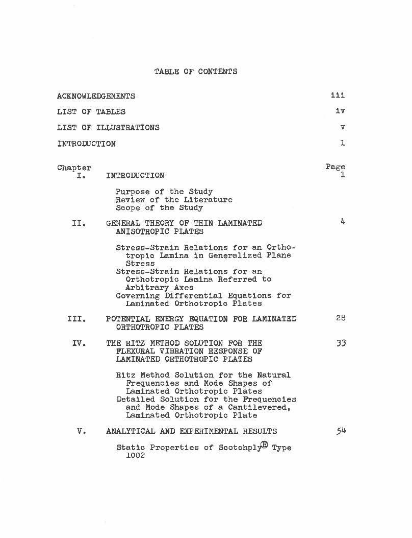
TABLE OF CONTENTS

ACKNOWLEDGEMENTS H iLIST OF TABLES ivLIST OF ILLUSTRATIONS vINTRODUCTION 1

Chapter PageI. INTRODUCTION 1Purpose of the Study- Review of the Literature Scope of the Study

IIo GENERAL THEORY OF THIN LAMINATED ^ANISOTROPIC PLATESStress-Strain Relations for an Ortho­tropic Lamina in Generalized Plane Stress

Stress-Strain Relations for an Orthotropic Lamina Referred to Arbitrary Axes

Governing Differential Equations for Laminated Orthotropic PlatesIII. POTENTIAL ENERGY EQUATION FOR LAMINATED 28

ORTHOTROPIC PLATESIV. THE RITZ METHOD SOLUTION FOR THE 33

FLEXURAL VIBRATION RESPONSE OF LAMINATED ORTHOTROPIC PLATESRitz Method Solution for the Natural

Frequencies and Mode Shapes of Laminated Orthotropic Plates

Detailed Solution for the Frequencies and Mode Shapes of a Cantilevered,Laminated Orthotropic Plate

V. ANALYTICAL AND EXPERIMENTAL RESULTS 5^

Static Properties of Scotchplji® Type 1002

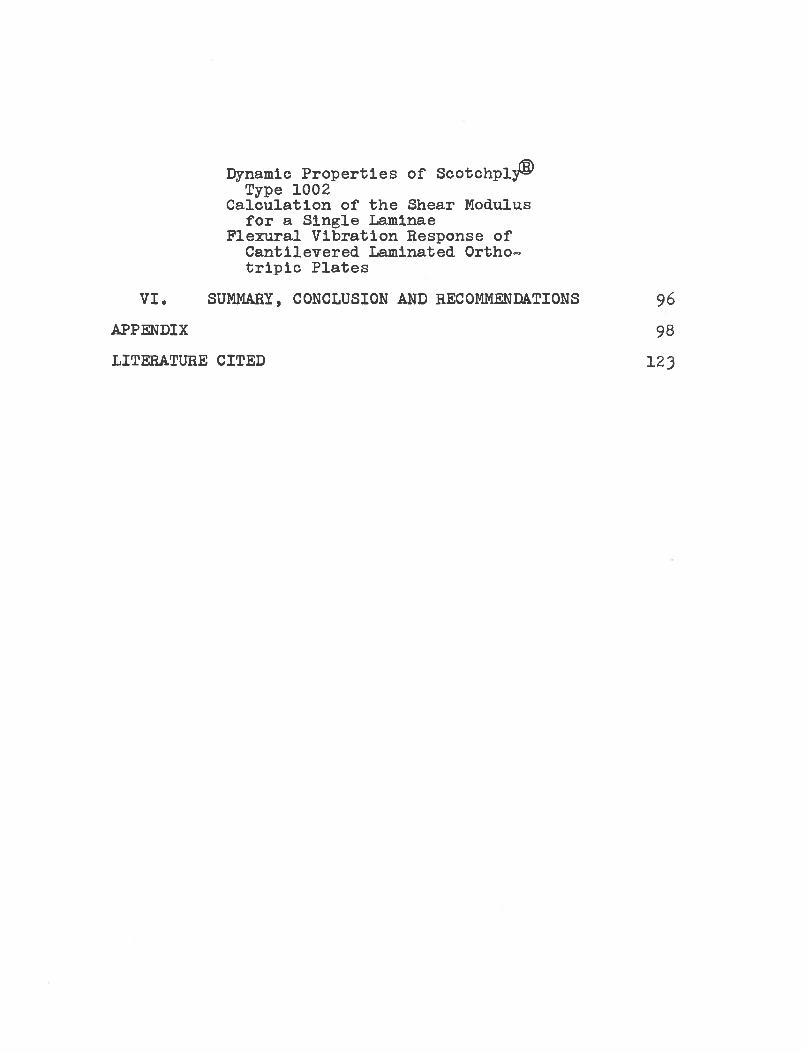
Dynamic Properties of Scotchply®Type 1002 Calculation of the Shear Modulus for a Single Laminae

Flexural Vibration Response of Cantilevered Laminated Ortho- triple Plates

VI. SUMMARY, CONCLUSION AND RECOMMENDATIONS APPENDIXLITERATURE CITED

9698

123

SUMMARY,

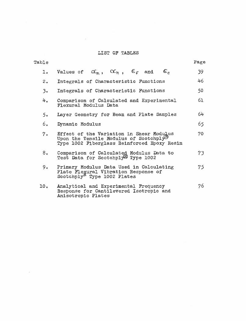
LIST OF TABLESTable Page

1. Values of , GC^ , £f and €c 392. Integrals of Characteristic Functions 463« Integrals of Characteristic Functions 504« Comparison of Calculated and Experimental 6lFlexural Modulus Data5o Layer Geometry for Beam and Plate Samples 646» Dynamic Modulus 657o Effect of the Variation In Shear Modulus 70Upon the Tensile Modulus of Scotchply^

Type 1002 Fiberglass Heinforced Epoxy Resin80 Comparison of Calculated Modulus Data to 73Test Data for Scotchply® Type 10029» Primary Modulus Data Used in Calculating 75Plate Flexural Vibration Response of

ScotchplyH Type 1002 Plates10o Analytical and Experimental Frequency 76

Response for Cantilevered Isotropic and Anisotropic Plates

m

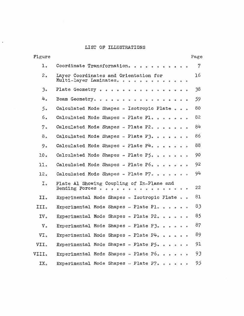
Figure1.20

3«k.

5o6.7.8,9°10 c 11c12 cIo

lieIIIcIV C VcVieVileVIIIc

LIST OF ILLUSTRATIONS

Coordinate Transformation0 » . 0 » » » c c »Layer Coordinates and Orientation for Multi-layer Laminates» o o o e e o e o e o oPlate Geometry o o o o o o o o o o o o o c oBeam Geometry o o o e o o o o o o o c o o o oCalculated Mode Shapes - Isotropic Plate o cCalculated Mode Shapes - Plate Pl» o c o » oCalculated Mode Shapes - Plate P2C » e o c cCalculated Mode Shapes - Plate P3« « » o « »Calculated Mode Shapes - Plate P -0 8 » c » cCalculated Mode Shapes - Plate P5» c c c « oCalculated Mode Shapes - Plate P6« , 0 o » cCalculated Mode Shapes - Plate P7o o o » c °Plate A1 Showing Coupling of In-Plane and Bending Forces o o o o o o o o o o o c o o oExperimental Mode Shapes - Isotropic Plate »Experimental Mode Shapes - Plate Plo o 0 o oExperimental Mode Shapes - Plate P20 » c « »Experimental Mode Shapes - Plate P3° c c <> oExperimental Mode Shapes - Plate P^e » » « oExperimental Mode Shapes - Plate P5° o « o »Experimental Mode Shapes - Plate P6» o o c »Experimental Mode Shapes = Plate P7« » <> o c

Page7

16oc 38 - 59o 80» 82 » 8k 0 86 c 88c 90 o 92 o 9 k

c 22» 81 o 83 . 85c 87 c 89 <, 91. 93c 95IX

CHAPTER I

INTRODUCTION

The behavior of anisotropic materials has been the object of much recent research® The high strength to weight ratio needed by aerospace structures has necessitated the use of exotic, composite materials which generally exhibit anisotropic behavior® These materials cannot be fully utilized unless analytical techniques are used which take maximum advantage of their anisotropic behavior®

The majority of the work now completed is in the area of static behavior of anisotropic materials® There has been extensive work done in the analytical theory of anisotropic plates and shells® A sufficient amount of experimental work has been done to verify the general theory of behavior of anisotropic materials®

Far less consideration has been given to the dynamic response of anisotropic materials® The importance of knowing the dynamic response of a material cannot be minimized® One of the current methods of analysis is to assume the material to be isotropic, solve the dynamic problem and then correlate the analytical dynamic response with experimental data taken with the anisotropic material®

2

The isotropic analysis will yield bounds for the response of the structure but at best it is a crude approximation in many cases„

In cases where the anisotropy of a material is quite strong it can be imperative to know the vibration response before the material can be safely and efficiently utilizedo

Purpose of the StudyThis study was intended to determine the vibration

response of laminated orthotropic plates» The vibration response was to be determined analytically and then verified experimentally0

Review of the LiteratureThe static behavior of anisotropic materials has

been extensively developed in the literature0 Two bookss one In Russian by Lekhnitskii (1) and one in English by Hearmon (2) have been written on the subject of anisotropic elasticity,, A comprehensive treatise covering the basic equations which apply to anisotropic plates and shells has been written by Dong9 Matthlesen9 Plster9 and Taylor(3) o

The forced flexural vibrations of sandwich plates has been analyzed by Yi-Yuan Yu (^)» The forced flexural

3

vibration response of orthotropic plates was determined by Hearmon (5)* Hearmon*s analysis produced a convenient closed form solution for plates which are orthotropic* in both ln-plane and bending loads,, Hearmon has two major assumptions which limit the versatility of his analysis„ First9 all boundaries of the plate have to be either clamped or simply supported,, Second, his analysis is restricted to plates which are orthotropic in bending and in general, plates constructed of ortho­tropic lamina are anistropic in bending„

Scope of the StudyThe analysis will develop, in general, all equations

necessary to determine the forced flexural vibration response of a plate constructed of orthotropic lamina,,Then, because a cantilevered plate is the simplest geometry to test experimentally, the boundary conditions for a cantilevered plate will be applied for the specific solution,,

All pertinent equations and data necessary to correlate the analytical development with the experimental work will be fully developed,.

*A complete definition and discussion of the terms orthotropic and anisotropic may be found in Chapter II, pages 25 and 26„

CHAPTER I I

GENERAL THEORY OF THIN LAMINATED ANISOTROPIC PLATES*

The theory of laminated anisotropic plates presented In this chapter will be restricted to anisotropic plates constructed of laminae which are orthotropic.

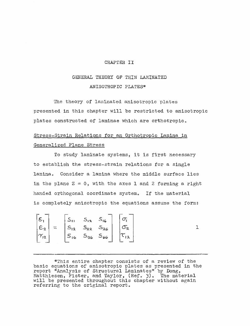
Stress-Strain Relations for an Orthotropic Lamina in Generalized Plane Stress

To study laminate systems, it is first necessary to establish the stress-strain relations for a single lamina. Consider a lamina where the middle surface lies in the plane Z = 0, with the axes 1 and 2 forming a right handed orthogonal coordinate system. If the material is completely anisotropic the equations assume the form:— -— _ —- — -G. •Sii 5, * S lG>

e* — •Si*Kb

__ - «— —1 — —

♦This entire chapter consists of a review of the basic equations of anisotropic plates as presented in the report "Analysis of Structural Laminates" by Dong, Matthiesen, Pister, and Taylor, (Ref. 3)• The material will be presented throughout this chapter without again referring to the original report.

1•Sii 5, * S lG>

■S i a■ Kb ~6><t> ^1*

£.£*'r.*

5

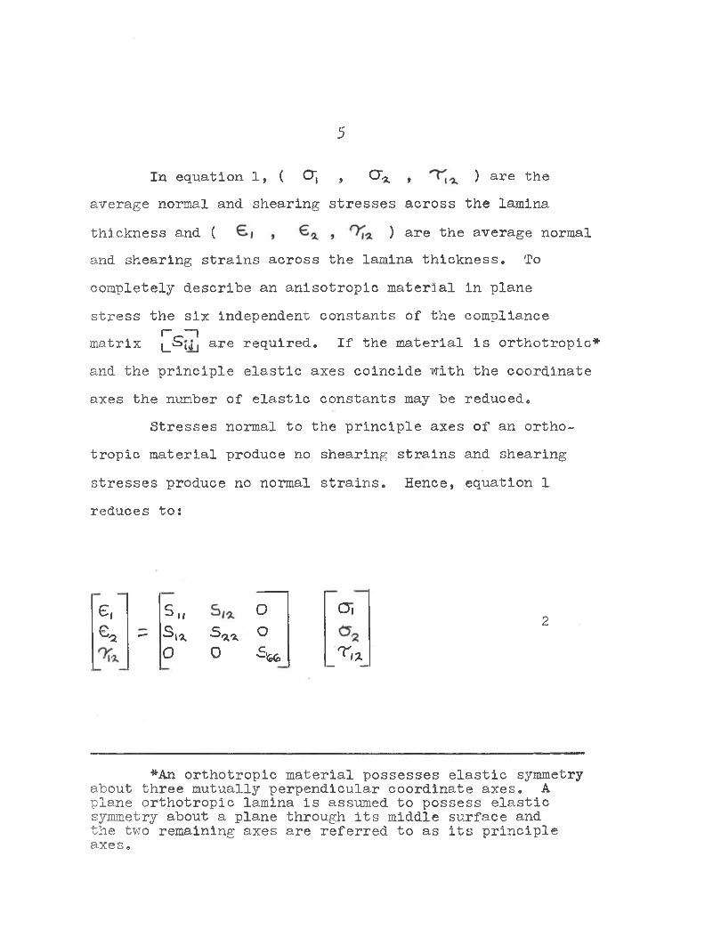
In equation 1, ( O", , CT , ) are theaverage normal and. shearing stresses across the laminathickness and ( ) are the average normaland shearing strains across the lamina thickness. Tocompletely describe an anisotropic material in planestress the six independent constants of the compliance

r — imatrix |_^uj are required. If the material is orthotropic* and the principle elastic axes coincide with the coordinate axes the number of elastic constants may be reduced.

Stresses normal to the principle axes of an ortho­tropic material produce no shearing strains and shearing stresses produce no normal strains. Hence, equation 1 reduces to:

e, s„ o cme* — Si-a.0 ■S** O 0 Ste _r '*_

*An orthotropic material possesses elastic symmetry about three mutually perpendicular coordinate axes. A plane orthotropic lamina is assumed to possess elastic symmetry about a plane through its middle surface and the two remaining axes are referred to as its principle axes.

2O■s** O0 Ste

cm

6

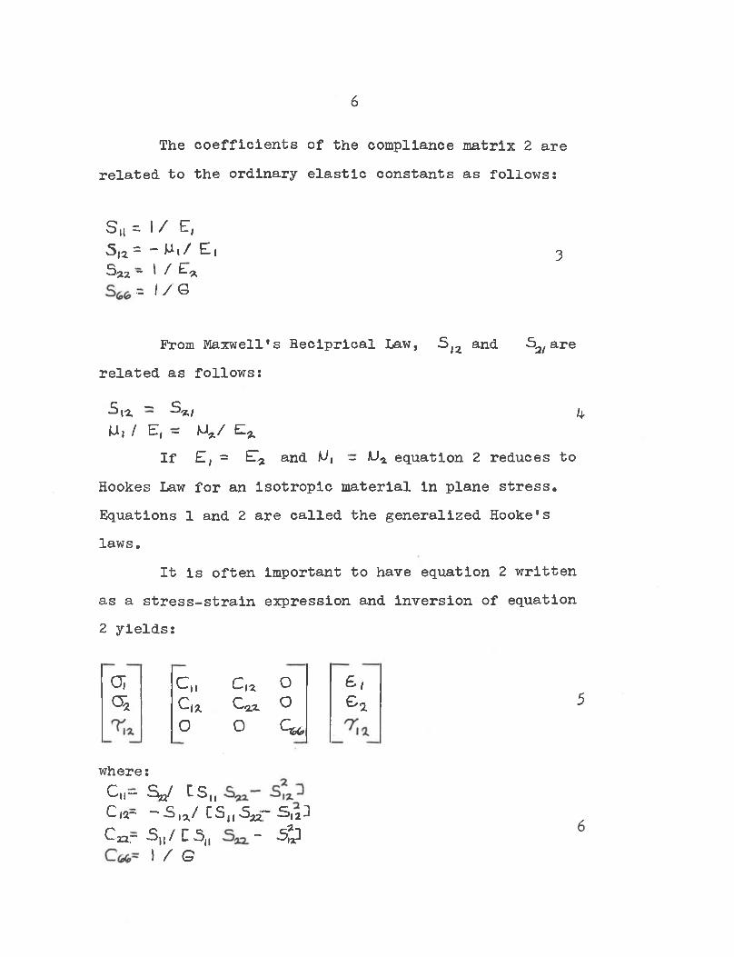
The coefficients of the compliance matrix 2 are related to the ordinary elastic constants as follows:

S„ = 1/ ET,5)2 = - Mi/ Ei 3

3^2 “ / -9.~ I / G

From Maxwell's Reciprlcal Law, S >2 and S2/are related as follows:

•Si-2. ~ S*/ 4U, / E, - M*/ E*

If £, = ET-2 and equation 2 reduces toHookes Law for an isotropic material in plane stress. Equations 1 and 2 are called the generalized Hooke's laws.

It is often important to have equation 2 written as a stress-strain expression and inversion of equation 2 yields:

0 ; C|| C|2 O S tQa. £”02. O e 20 0 Cft,

where:Cii— •Sq/ £S,,Cicr --S,*/ CS(,622“ S,2 Car 5 u/ C 5 (I - 5 ^

1 / G6

5Oicr*

s te 2

iJI - w*

?

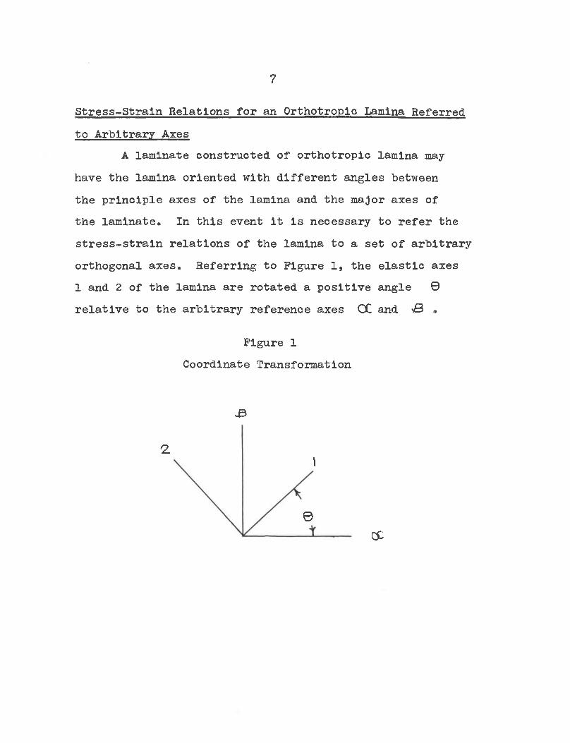
Stress-Strain Relations for an Orthotropic Lamina Referred to Arbitrary Axes

A laminate constructed of orthotropic lamina may- have the lamina oriented with different angles between the principle axes of the lamina and the major axes of the laminate. In this event it is necessary to refer the stress-strain relations of the lamina to a set of arbitrary orthogonal axes. Referring to Figure 1, the elastic axes 1 and 2 of the lamina are rotated a positive angle © relative to the arbitrary reference axes OC and & .

Figure 1 Coordinate Transformation

3

2.

ec©

\

8

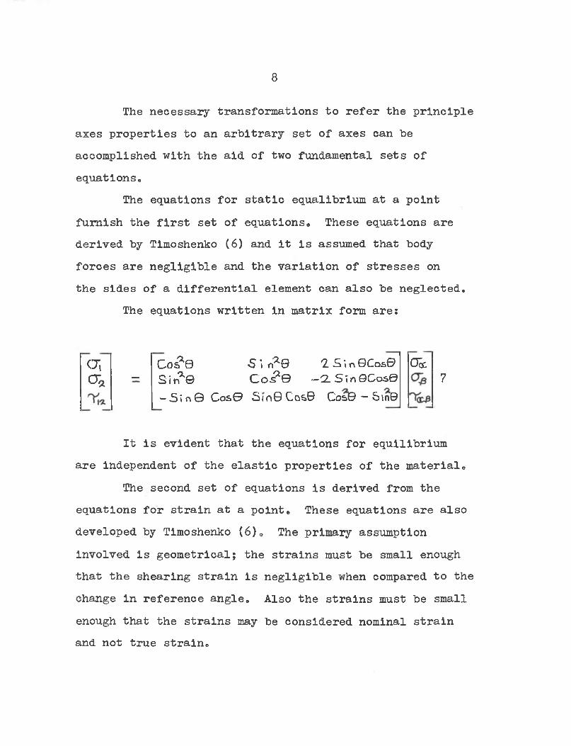
The necessary transformations to refer the principle axes properties to an arbitrary set of axes can be accomplished with the aid of two fundamental sets of equations.

The equations for static equallbrium at a point furnish the first set of equations. These equations are derived by Timoshenko (6) and it is assumed that body forces are negligible and the variation of stresses on the sides of a differential element can also be neglected.

The equations written in matrix form are:

<T, Cosa0 •S i n^B *2 S in QCosO OkO'* — Sin*© C o ^ 0 —2. S in ©Cos©

— S in © Cos© Sir>9 Cos© Cos© - Stn©

It is evident that the equations for equilibrium are independent of the elastic properties of the material.

The second set of equations is derived from the equations for strain at a point. These equations are also developed by Timoshenko (6). The primary assumption involved is geometrical; the strains must be small enough that the shearing strain is negligible when compared to the change in reference angle. Also the strains must be small enough that the strains may be considered nominal strain and not true strain.

7

9

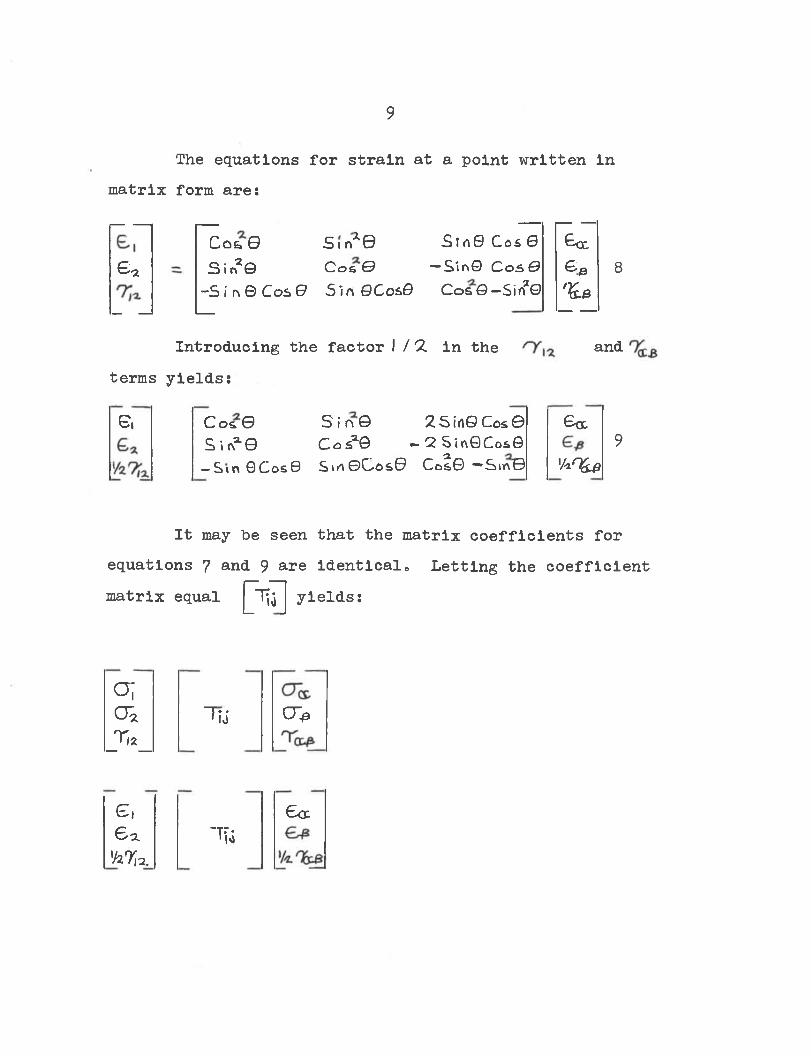
The equations for strain at a point written in matrix form are:— — — — — -

C o & Q SirV2-© S i n0 Cas 0 koce * Sin2© C o b & — SinG C o s 0 e *

—S i r\ © Cos © Sin GCosG Cos©-Sin2© 'S*__ _ __ —

Introducing the factor I / 'Z in the andterms yields:

e. Cos© S in © 25irt© Cos© ©QCSin2-© Cosa0 - 2 SinQCosG-S in 0Cos0 S\n©Cos0 Cal© — Sin© V<L%#

It may he seen that the equations 7 and 9 are identical matrix equal [^Tj yields:

matrix coefficients for 6 Letting the coefficient

o ;CTa

_T/2_T?J o >

G,6 afcr*.

"Tfo£<x

8

9

10

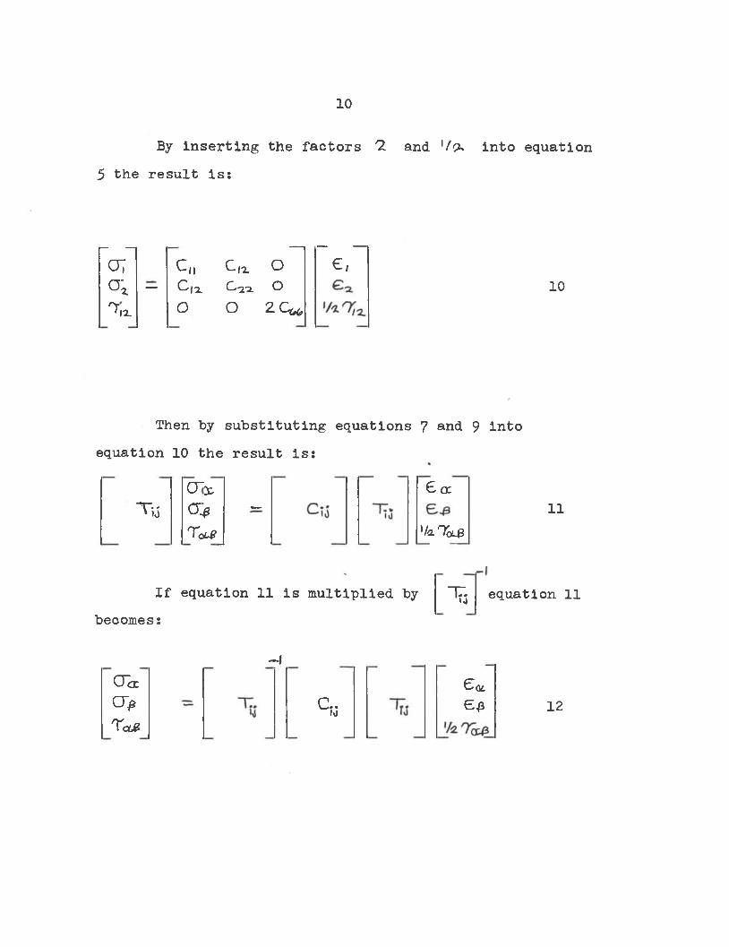
By inserting the factors 'I and '/c into equation 5 the result is:

— — — — --07 c„ C,x O €,Ok — C,a C-xx OTix O o z c «

10

Then by substituting equations 7 and 9 intoequation 10 the result is:

0"x 6 ccOf —raf_ '/xTcxe

11

If equation 11 is multiplied by becomes:

t 3 equation 11

CTocCT>Ted?

12

-I

C..10C qcee

Ttf

11

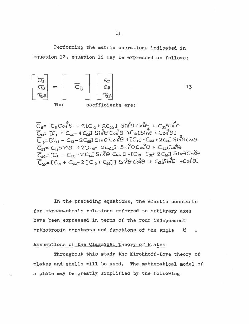
P e r fo r m in g th e m a tr ix o p e r a t io n s in d i c a t e d in

e q u a t io n 1 2 , e q u a t io n 12 may b e e x p r e s s e d a s f o l l o w s :

Cb: £cco# = C-*'--10

The c o e f f i c i e n t s a r e :

C„= C „C o*0 + ^ZCC,a+2C 463 5 7*0 CosQ + C^.Si *0 C«r CC„ + Qq.—4 C^l S '*0 Co*0 vC^^Sln© + Cos&J ^C|4,= CC11 — C|2— Si n0 Co^0 4 r C |o . ~ C 'ZCtf] S(nQ Cos>Q O jjr C „5 i^ e + 2CC,**- 2C 66D SirfeCos^e + CzzCoJe 0*6= CCn - C l2- 2 C^] Sf n 0 Cos 0 +CCiz-C 22+ 2 C ^ ] S 'iaQ Co^ C^CCm* Cnr^lC,Z+C«n SfiBCole + QsCS.rfe +Cotel

In t h e p r e c e d in g e q u a t io n s , t h e e l a s t i c c o n s t a n t s

f o r s t r e s s - s t r a i n r e l a t i o n s r e f e r r e d t o a r b i t r a r y a x e s

h a v e b e e n e x p r e s s e d in te r m s o f t h e fo u r in d e p e n d e n t

o r t h o t r o p ic c o n s t a n t s and f u n c t i o n s o f t h e a n g le 0

A ssu m p tio n s o f t h e C l a s s i c a l T h eory o f P l a t e s

T h rou gh ou t t h i s s tu d y t h e K ir c h h o f f -L o v e t h e o r y o f

p l a t e s and s h e l l s w i l l be u s e d . The m a th e m a tic a l m od el o f

a p l a t e may be g r e a t l y s i m p l i f i e d by t h e f o l l o w i n g

13

12

assumptions; 1. Normals to the undeformed middle surfaceremain normal to the deformed middle surface and suffer no extension,, 2. The thickness of the plate is small in comparison to the lateral dimensions.

It is also assumed that the plate is in a state of generalized plane stress and strains and displacements of second or higher order are neglected in comparison with first order terms.

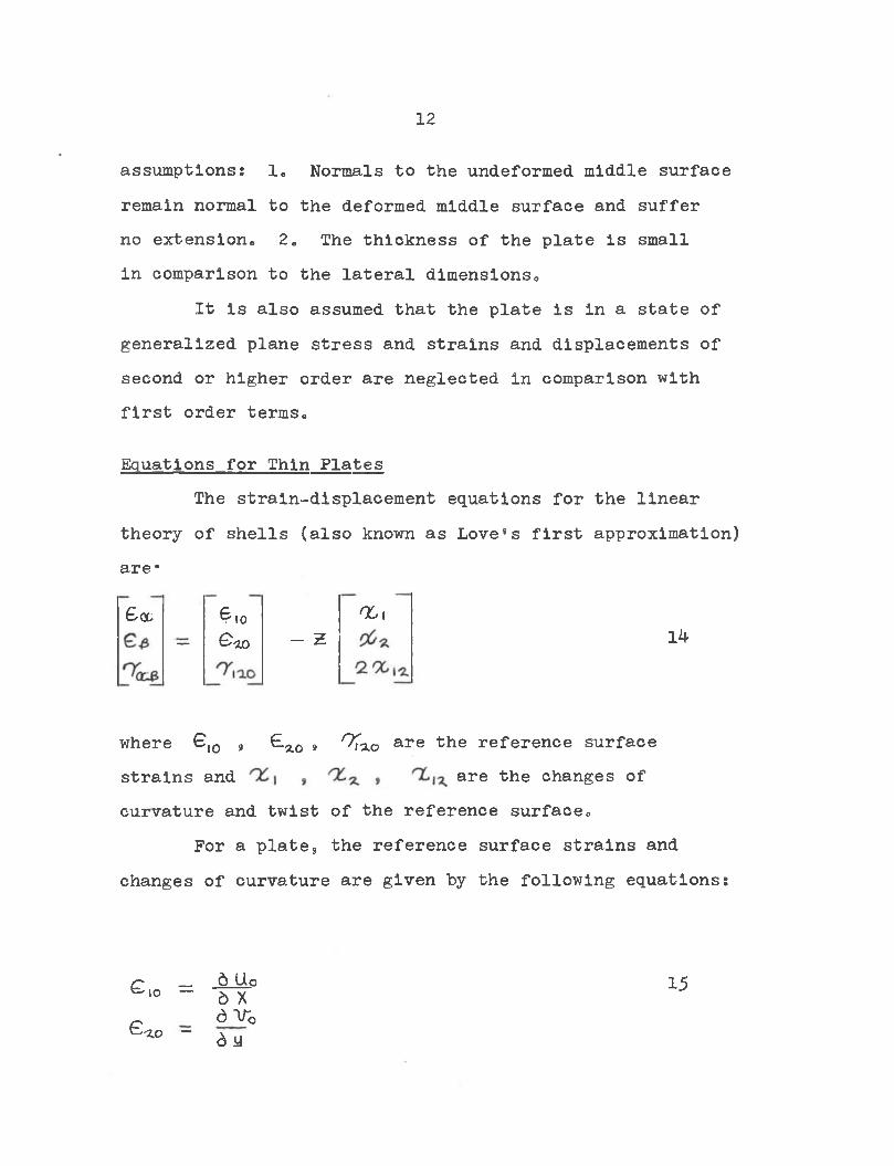
Equations for Thin PlatesThe strain-displacement equations for the linear

theory of shells (also known as Love8s first approximation) are*

G od G 10 no i— G .0 - Z

where 6 |0 , €lzo 9 /?fao are the reference surfacestrains and are the changes ofcurvature and twist of the reference surface.

For a plate9 the reference surface strains and changes of curvature are given by the following equations:

p — 6 Uo^ io — 6 XdirQG-xo - 6 y

15

14

13

^IZO

X ,

x *

X,*

d V c d U 0<a X e>y<y*uja x*d^Wa y2eTiw ax oa

15

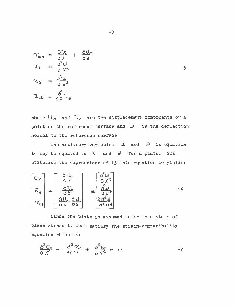
where U.0 and ~l£ are the displacement components of a point on the reference surface and W is the deflection normal to the reference surface.

The arbitrary variables GC and in equation14 may be equated to X and y for a plate. Sub­stituting the expressions of 15 into equation 14 yields:

r da0 1 rex 6 X dX2ea = <5ir0oy

2awdb*

r~ l“=

6U&, 6U0ox oy oxaySince the plate is assumed to be in a state of

plane stress it must satisfy the strain-compatibility equation which is:

_ afrxy _o x2 ax oy d y* ~ o i?

16

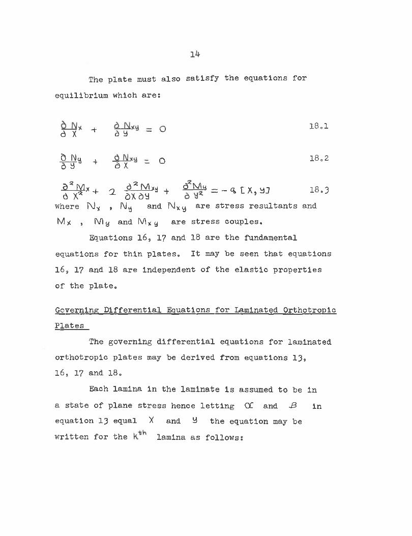
The plate must also satisfy the equations for equilibrium which are:

where iXJ* , My and N Xy are stress resultants and M / , (V\y and fV\x a are stress couples.

Equations l6s 17 and 18 are the fundamental equations for thin plates. It may be seen that equations l69 17 and 18 are independent of the elastic properties of the plate.

Governing Differential Equations for Laminated Orthotropic Plates

The governing differential equations for laminated orthotropic plates may be derived from equations 13s l6j 17 and 18.

Each lamina in the laminate is assumed to be in a state of plane stress hence letting OC and -B in equation 13 equal "X and ^ the equation may be written for the

18.1

O 18.2

18.3

lamina as follows

6 i + ay ~ u

5 IMu .6 y d X

-S-f_Mx i n a^ Myj , 6 My — _ q. [ X Ml6 ^ + 2 dxe>y + ~ ^ LA,yj

15

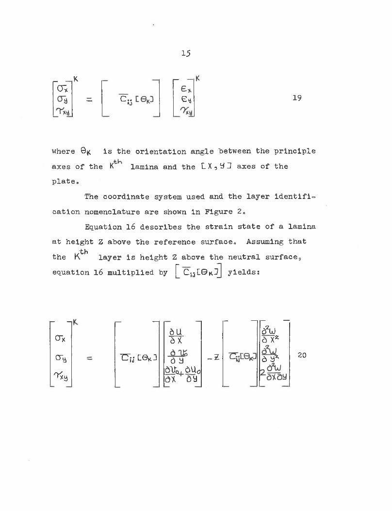
_ K r— —cr*

— C;* €■4

where ©|c Is the orientation angle "between the principle axes of the K lamina and the L X ,'d J axes of the plate.

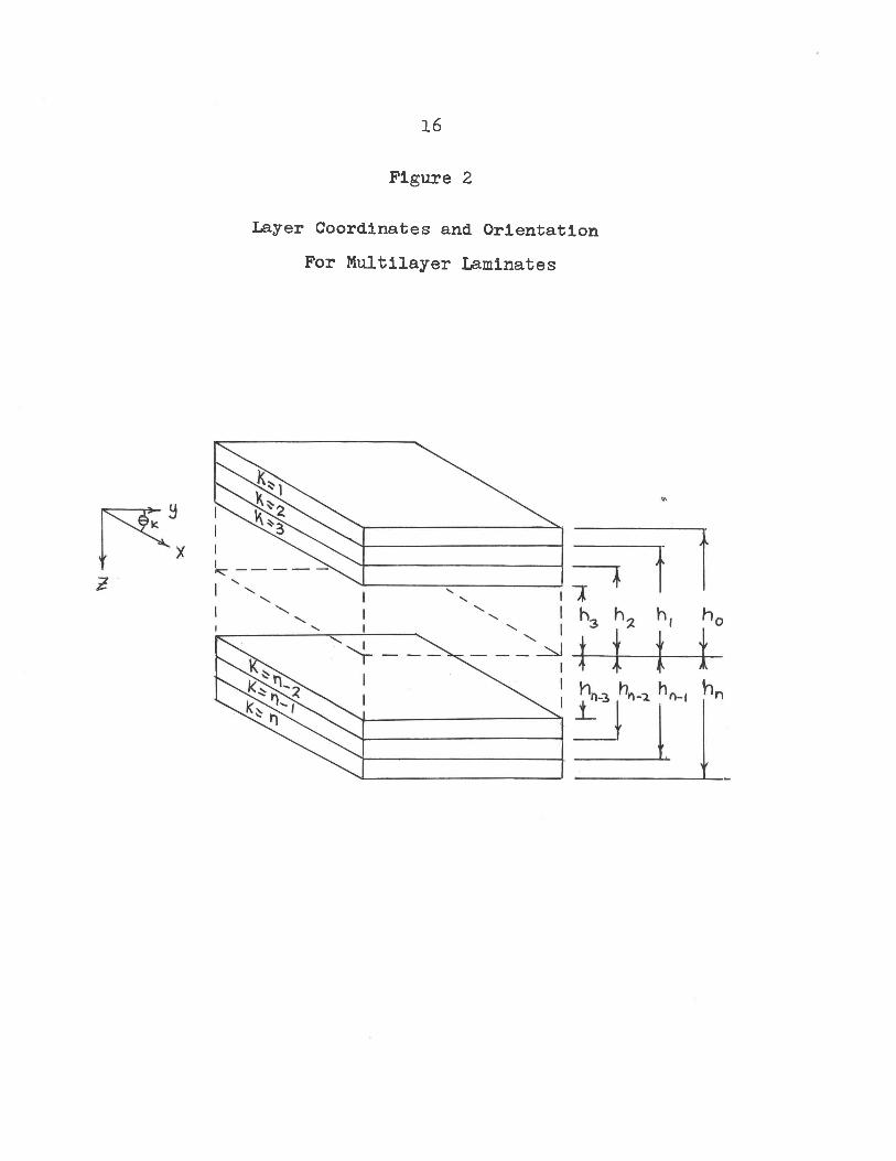
The coordinate system used and the layer identifi­cation nomenclature are shown in Figure 2.

Equation 16 describes the strain state of a laminaat height Z above the reference surface. Assuming that

,/ththe r\ layer is height Z above the neutral surface9 equation 16 multiplied by f C 13L© k ] yields?

i— 1 — — — — - -da dfucr* dX 6 X2

TTfj C©«3 6 y 6 6V0, 6Uodt ©y

19

20_Z<*»^ 3

16

Figure 2

Layer Coordinates and Orientation For Multilayer Laminates

h3 h2 h, h0

<V, hn

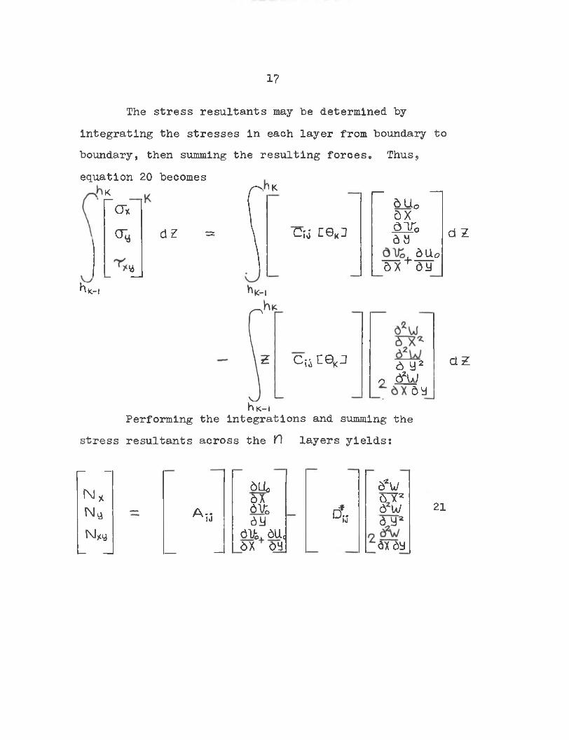
17

The stress resultants may he determined by integrating the stresses in each layer from boundary to boundary, then summing the resulting forces«, Thus, equation 20 becomes

K r ' K — —~CTx 6 U 0

axCTy

“ * \ C r j ceKi] air0aa

au0 a x f ay,1

__1

d Z

c u c e . j 6 y2 o tfy

dy

d Z

h K—iPerforming the integrations and summing the stress resultants across the fi layers yields:

— —N*

— /\ - * 10

_ _ __ _

6Lio6X6Uoay

6V0, 6LLCax ay

d!.Id

a*wa r 26 Wa y 2 ax ay

21

Htc-i

2

N*N yN/y

18

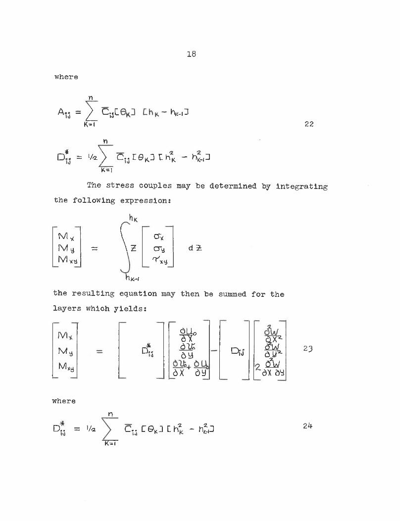
where

nA-* - 2 _ ^13 hie-i3

K=l 22m

D*. = '/« > c..reK3 £>v ~ >\-PK=l

The stress couples may be determined by integrating the following expression:

d i

h«-ithe resulting equation may then be summed for the layers which yields:

M y \ CTyM y = \ z CTyMyy r*'%SA

M-M,M <8

*D.,&dVZay

dx ay

D;'ivJ ay<2 <£wax ay

23

where

D.. = i/«

n

K=iC,. r© Kj Ch* - hjp 24

19

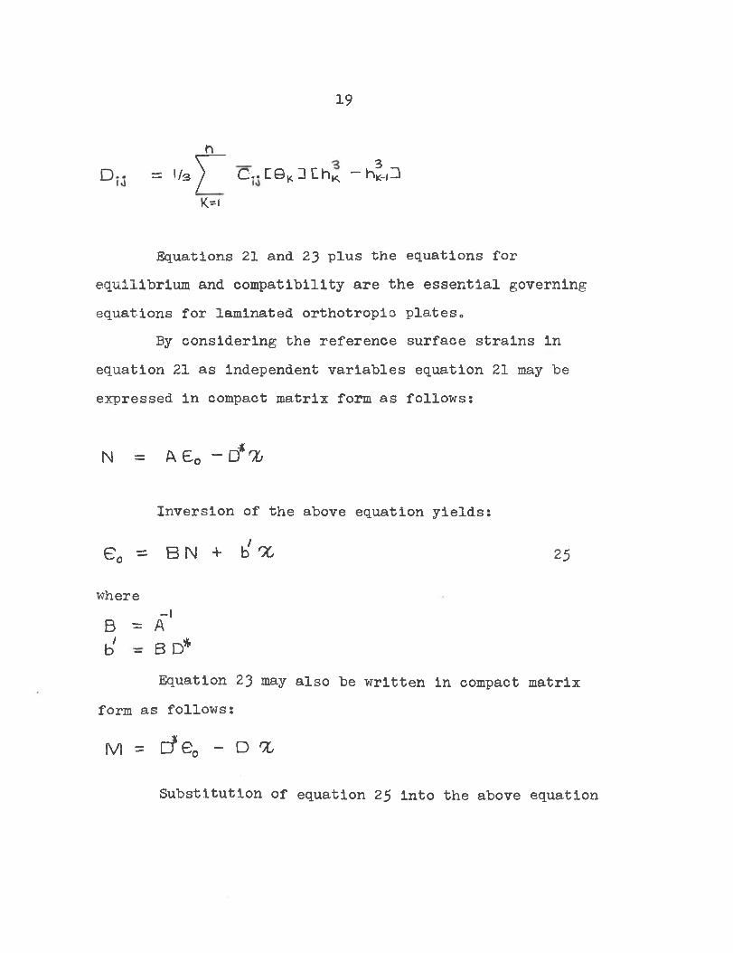
h= 1/3 J C.* C©K II L h * -ht,3

K=i

Equations 21 and 23 plus the equations for equilibrium and compatibility are the essential governing equations for laminated orthotropic plates.

By considering the reference surface strains in equation 21 as independent variables equation 21 may be expressed in compact matrix form as follows:

N = A S0 -0*%

Inversion of the above equation yields:

e0 = B N + b'x 25where

-lB = A b' - B D*

Equation 23 may also be written in compact matrix form as follows:

m = d e c - d ccSubstitution of equation 25 into the above equation

b N + d % 26

20

yields:

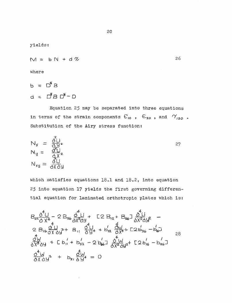
(VI =

where

b ~ D* B

d - D*B D *~ D

Equation 25 may be separated into three equations in terms of the strain components G |0 , £ ao , and Orno . Substitution of the Airy stress function:

NN

N

7dL) S3* d2U?U

“ ax ay

y - y =

27

which satisfies equations 18,1 and 18,2, into equation 25 into equation 17 yields the first governing differen­tial equation for. laminated orthotropic plates which is:

R _ o o d U

B „ 0LJ

B,x + a4u

4awa F a y

,fcax ay~

a x 2ai/

+ b'z |y4+ C2 ba4, -k^P

■(■ E b 11 ■+ b%j Q b^D46 W

ax2 ay2+ E Q b)(j

a4w ax ay + b a4w ,

2/ a y 4 o

28

21

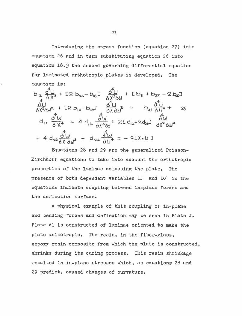
Introducing the stress function (equation 27) into equation 26 and in turn substituting equation 26 into equation 18.3 the second governing differential equation for laminated orthotropic plates is developed. The equation is:

Equations 28 and 29 are the generalized Poisson- Kirchhoff equations to take into account the orthotropic properties of the laminae composing the plate. The presence of both dependent variables U and U/ in the equations indicate coupling between in-plane forces and the deflection surface.

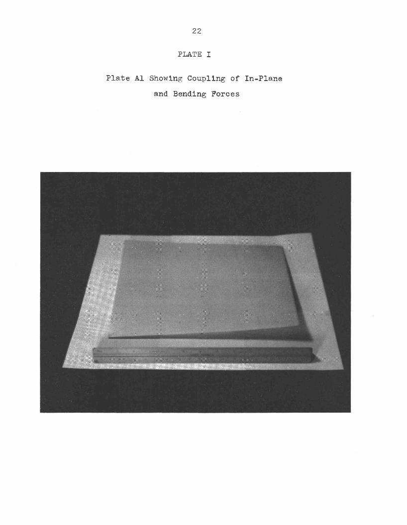
A physical example of this coupling of in-plane and bending forces and deflection may be seen in Plate I. Plate A1 is constructed of laminae oriented to make the plate anisotropic. The resin, in the fiber-glass, expoxy resin composite from which the plate is constructed, shrinks during its curing process. This resin shrinkage resulted in in-plane stresses which, as equations 28 and 29 predict, caused changes of curvature.

22

PLATE I

Plate A1 Showing Coupling of In-Plane and Bending Forces

23

It is beyond the scope of this study to consider the vibration response of anisotropic plates. For certain lamina orientations equations 28 and 29 simplify so that a solution is obtainable.

The first of these specialized orientations produces a homogeneous anisotropic plate. This classification describes a laminated plate made from pairs of the same orthotropic laminae. The laminae are oriented such that one is the same distance above the reference surface as the other is below the reference surface.

The principle axis of both laminae run in the same direction. For this orientation the Dfj vanish and equation 28 and 29 reduce to:

+ H 2 B (2_U 6X*6yz 304

CZDlx+4Dm3 ax* ay* 314A W

q/ix ,yD

24-

Plates of this type are equivalent to homogeneous anisotropic plates. The vibration response of plates of the type described by equations 30 and 31 will be considered in this study.

Further specialization is possible by having the laminae pairs at +4-5° from the major (X 9 y ) axes of the plate. In this case the elastic constants becomes

A„ —

A (fc-Bn - BxlB \<o— B'lCoD /( D 1 -3.

D* - D ig,Equations 30 and 31 become:

B 64U 6*11II y ? + C B ^ 2 ^ 36 U = o dy4

32

4 +D„ + 4 D,6 y + C 2 D (1 + 4 D ^ J

4 D % r i ^ + D" # = - q t x ’a3

46 W 33

Equations 32 and 33 are the equations for a plate which is orthotropic in in-plane effects and anisotropic in bending.

If all of the laminae pairs are oriented parallel

o

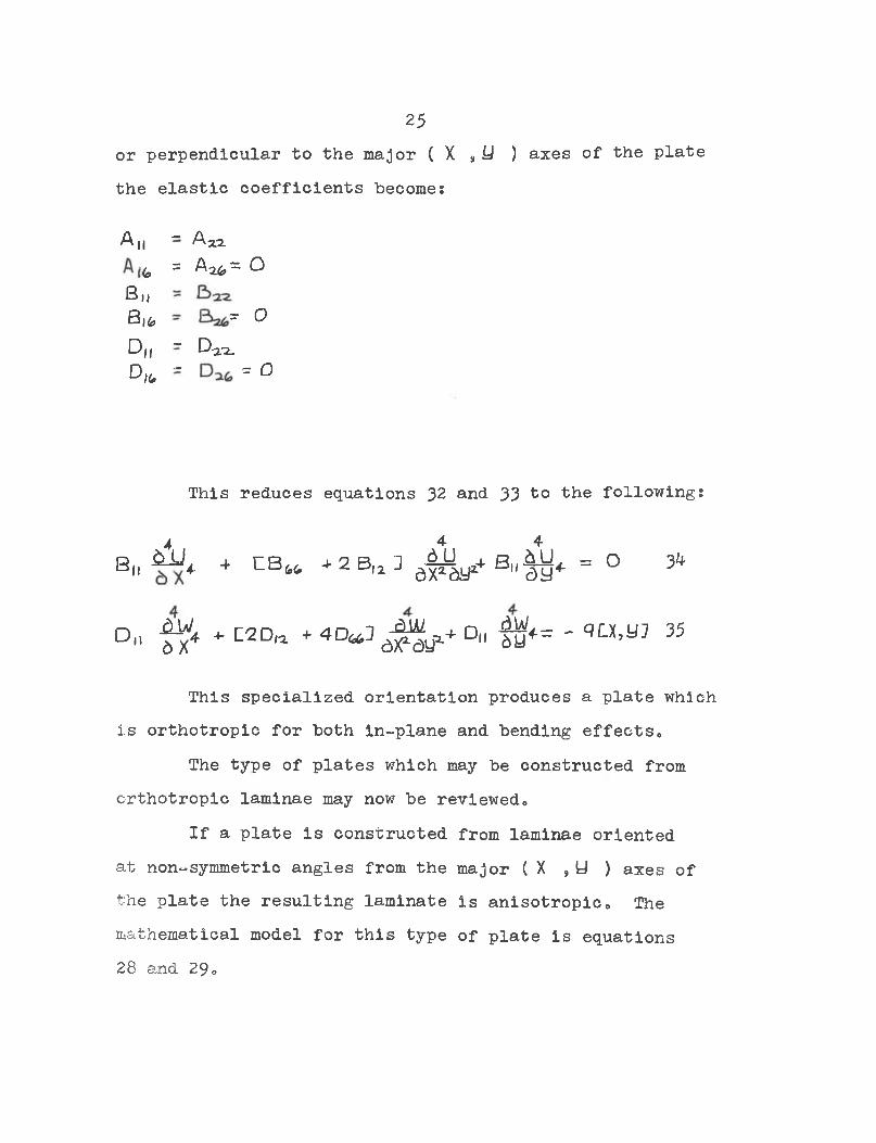
25or perpendicular to the major ( X »U ) axes of the plate the elastic coefficients become:

A h — A xx

(c = A x(o~

B „Bifc

D )( - D-iU.D * —

This reduces equations 32 and 33 to the following:

B„ &><. 4 CB* -*1 2 Bi2 J d B „ ^ = O 34

d„ ^ 4 * l2d,i + 4 c u ] ^ + d„ f^4= - qa,yj 35

This specialized orientation produces a plate which is orthotropic for both in-plane and bending effects.

The type of plates which may be constructed from orthotropic laminae may now be reviewed.

If a plate Is constructed from laminae oriented at non-symmetric angles from the major (X 9 y ) axes of the plate the resulting laminate is anisotropic. The mathematical model for this type of plate is equations 28 and 29»

= o

- 0

~ o

26

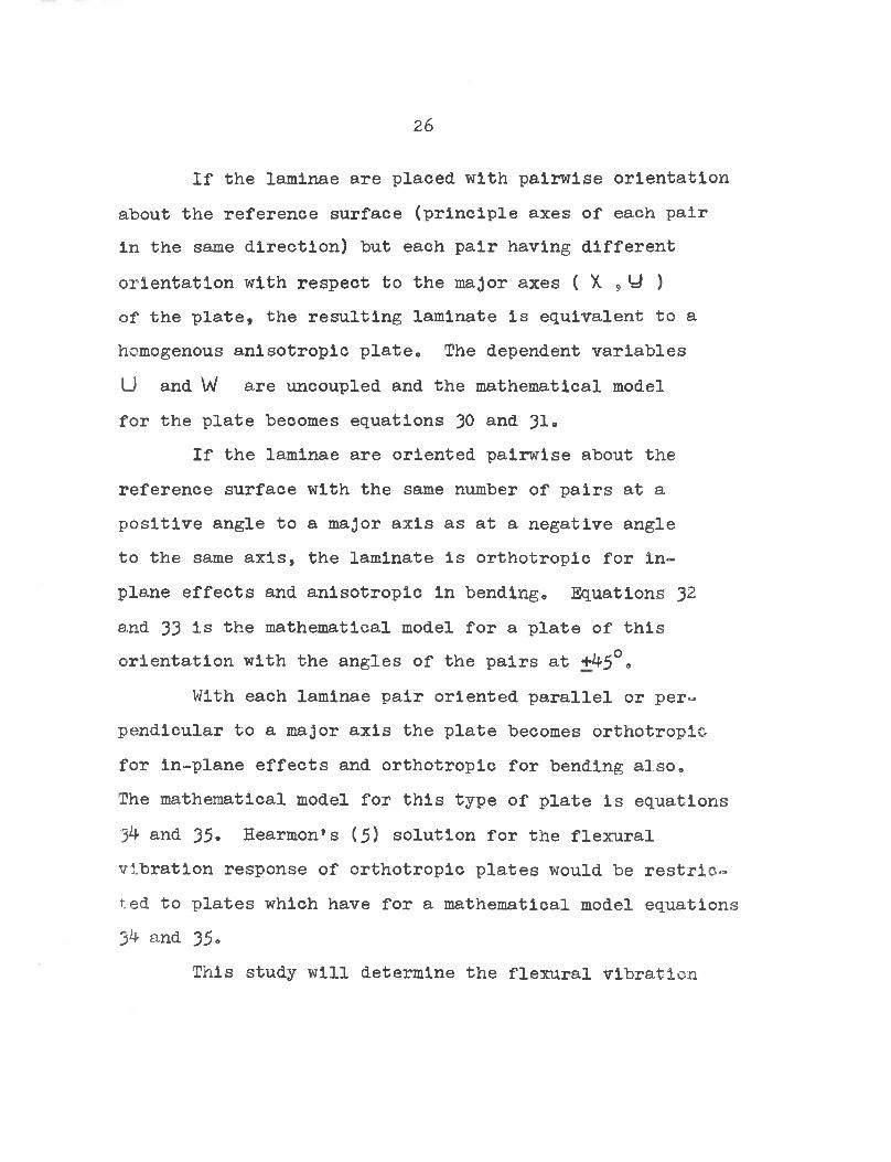
If the laminae are placed with pairwise orientation about the reference surface (principle axes of each pair in the same direction) but each pair having different orientation with respect to the major axes ( X. 9U ) of the plate, the resulting laminate is equivalent to a homogenous anisotropic plate. The dependent variables LJ and W are uncoupled and the mathematical model for the plate becomes equations 30 and 31•

If the laminae are oriented pairwise about the reference surface with the same number of pairs at a positive angle to a major axis as at a negative angle to the same axis, the laminate is orthotropic for in­plane effects and anisotropic in bending. Equations 32 and 33 is the mathematical model for a plate of this orientation with the angles of the pairs at +^5°»

With each laminae pair oriented parallel or per­pendicular to a major axis the plate becomes orthotropic for in-plane effects and orthotropic for bending also.The mathematical model for this type of plate is equations 3^ and 35* Hearmon’s (5) solution for the flexural vibration response of orthotropic plates would be restric­ted to plates which have for a mathematical model equations 3^ and 35.

This study will determine the flexural vibration

2?

response for plates which have for a mathematical model equations 30 and 31* Plates which have for a mathemati­cal model equations 32 and 33» and 33 and are a specialization of those which have equations 30 and 31 for a mathematical model and hence will be included in this study.

3^

CHAPTER III

POTENTIAL ENERGY EQUATION FOR LAMINATED ORTHOTROPIC PLATES

This study will determine the flexural vibration response of laminated orthotropic plates* As outlined at the conclusion of Chapter II the study will be restricted to those plates which are uncoupled in bending and in-plane effects. The mathematical model for this type of plate is equations 30 and 31•

Solution of equations 30 and 31 will not be attempted directly. The Ritz method will be used. The details of this solution technique are found in Chapter IV.

In order to use the Ritz method a potential energy term must be developed for the plate. If it is assumed that the laminae of the plate are pairwise oriented about the reference surface and the principle axes of each lamina in a pair are at the same angle with respect to the major axes of the plate, equation 23 may be expressed as follows:

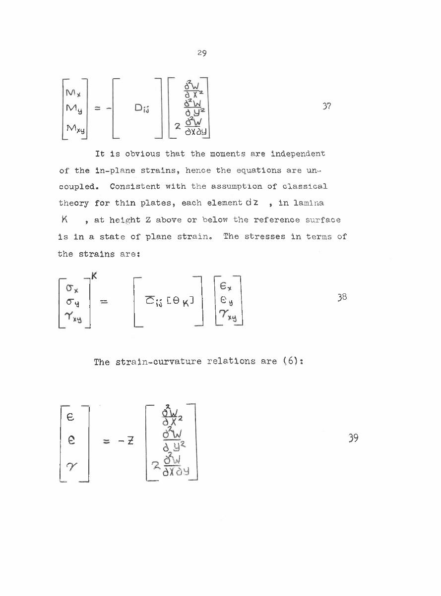
ay ay

It is obvious that the moments are independent of the in-plane strains, hence the equations are un­coupled. Consistent with the assumption of classical theory for thin plates, each element d2 , in lamina K , at height Z above or below the reference surface is in a state of plane strain. The stresses in terms of the strains are:

IS

cr* — c ii c e * } e*

The strain-curvature relations are (6):

0

e

nr-z

3?

38

39

29

M y :Mj<y

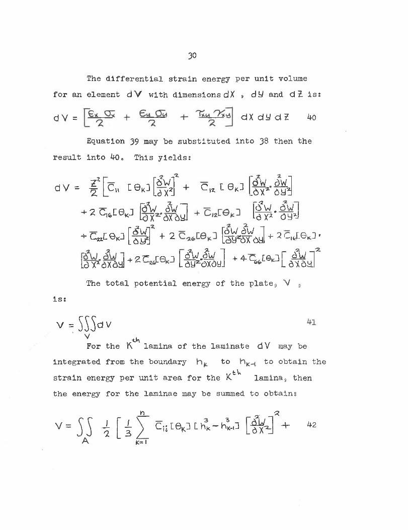
30

The differential strain energy per unit volume for an element d V with dimensions dX » dt/ and d 2. is:

d V = d X d y d 2 40Equation 39 may be substituted Into 38 then the

result into 40„ This yields:

dV= 1 c„ c e K]2 C lfeC0KJ

yT:2Ja w l

"dX dyj

6 W L3X21 + C (ZL 0 k3 ~dw aw

_ax* ayakgw.awlLax2 oy*J

+ c ^ c e ^ [fg] + 2 c ^ c e Ki[ t ^ J + 2 ■

,z r r « 1 i w . l w 1 4. 4 . 0 re 3 r i wLax1 ax ad + Lay^axayJ “6fcl.-2 . _.-2.

Laxay.The total potential energy of the plate9 V

is:

v = 5 ^ d v v <*,For the K. lamina of the laminate dV may be

integrated from the boundary to to obtain thetUstrain energy per unit area for the X. laminas then

the energy for the laminae may be summed to obtain?

JL1

C ISL © ^ LhK~ht.33a- 42

312 C,ateK] C h? - + 2 c l(j:eK ] L ^

6 W £ WLax ax ay.

" i w . - & 1_ax2 ax ay]

C,aC0 3 L I'V - Vv,3 + QaL©k]Chl-h^Hefw.cfw d y 2axay4 2 c^ceK3 t hi- hjf-P [j

r & i w 1 + 2 L hi - Vi,llLe>x2axay] 742 4 2 C l(>CeK 3thl-ht3d \ / . £ w ay2 ax ay

4 C6feC0iJI C h it hi JJ r ^ w TLaxayJ a x d y

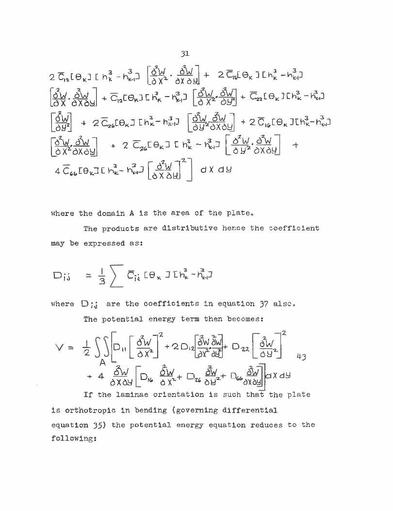
where the domain A is the area of the plate,.The products are distributive hence the coefficient

may be expressed as:

D,-j - 3 ) C;i C0K

where Dfj are the coefficients in equation 3? aXso0 The potential energy term then becomes:

V = -k

A LD iir S w

axa

-,-z+ Q. Dtz aw aw D ix

Svj n aw n aw q Jw 0,6 ax^ a ay"2- <3xay

d Uay^j i3

dX dyaxayIf the laminae orientation is such that the plate

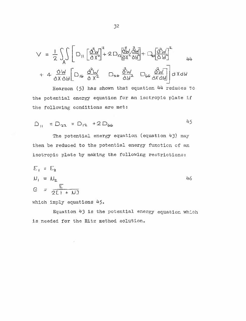
is orthotropic in bending (governing differential equation 35) the potential energy equation reduces to the following:

32

v - i S S

'->1ols 1 __ -z+ 2, D|26w.Sw + Qa aVf

A+. * 6W 1

1 □ cfu D-2.6)Svj n £w~|

^ dXdUJHearmon (5) has shown that equation 44 reduces to

the potential energy equation for an Isotropic plate If the following conditions are met:

D„ = D ^The potential energy equation (equation 43) may

then be reduced to the potential energy function of an isotropic plate by making the following restrictions:

E, = ET*JU, = 46r _ ______' 2L1 + AJUwhich imply equations 45«

Equation 43 is the potential energy equation whichis needed for the Ritz method solution

d X d t /

44

CHAPTER IV

THE RITZ METHOD SOLUTION FOR THE FLEXURAL VIBRATION RESPONSE OF LAMINATED

ORTHOTROPIC PLATES

The method developed by Ritz (7) was chosen to obtain the flexural vibration response of laminated orthotropic plates. Ritz (7) used the method to calculate the frequencies and nodal patterns for an isotropic plate with all four edges free. The technique was used by Xoung (8) to calculate the frequencies and nodal shapes for rectangular isotropic plates with combinations of free and clamped edges. Barton (9) applied the Ritz Method to determine the frequencies and nodal patterns for rectangular and skew cantilevered isotropic plates.

The Ritz Method is an approximate technique; it gives the upper bounds for the natural frequencies and the approximate mode shape for each frequency. The convergence and accuracy of the Ritz Method is discussed by Kantorovich and Krylov (10). The chief disadvantage of the Ritz Method is that the accuracy of the results cannot be determined with certainty.

In general, the restrictions on the type of equation

3^

the Ritz Method may be applied to are few. The method consists of finding an "admissible function" i.e., a function which satisfies the artificial boundary condi­tions, For a plate, the artificial boundary conditions are the slope and deflection boundary conditions, A finite series is formed with the products of arbitrary coefficients and the "admissable function". The solution series is substituted into the differential equation and partial derivitives are taken with respect to each coeffi­cient, This results in as many equations as there are coefficients, hence the arbitrary coefficients may be determined. With the arbitrary coefficients determined the series is then forced to act like a solution to the differential equation. For an "admissible function", Kantorovich and Krylov (10) prove that if an infinite number of terms are taken in the series, the process forces the series to converge and be an exact solution. Unlike Fourier Series solutions the series of admissible functions need not converge. Even though the Ritz Method provides a method for which the solution series need not converge, the difficulty in finding a good "admissible function" makes the technique difficult toapply

35Rltz Method Solution for the Natural Frequencies and Mode Shapes of Laminated Orthotropic Plates.

The first step in solving the problem of the flexural vibration response of laminated orthotropic plates is to determine the governing differential equation*

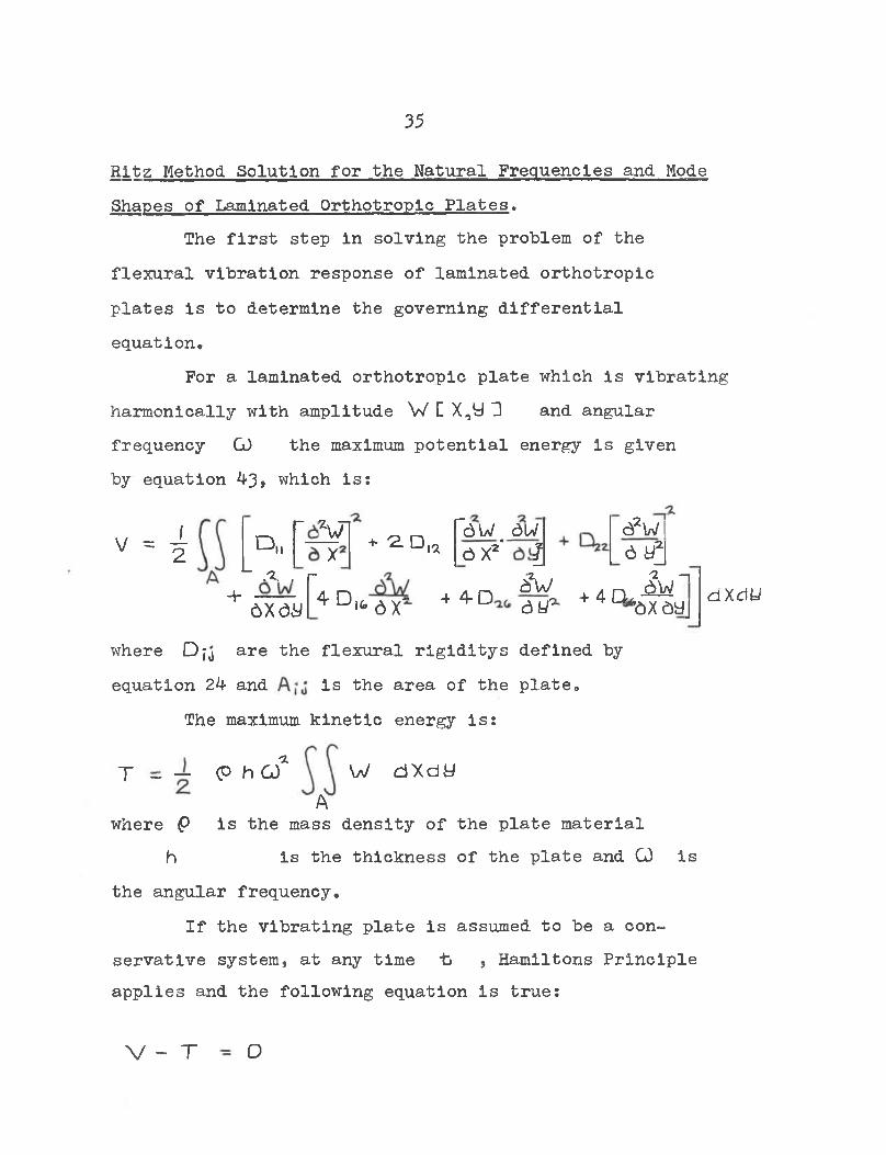
For a laminated orthotropic plate which is vibrating harmonically with amplitude W [ X,t)3 and angular frequency G) the maximum potential energy is given by equation A3, which is:

v - i D m>

*

L ___L A , r-

+ 2. □ n

+ 6X&y ’I* 6X'4Di,

rd W au 6 X2* I

dfw

62W|

4 4-D ay" + 4 CLa y^

2 —im’axayj aXdU

where Djj are the flexural rigiditys defined by equation 2k and is the area of the plate.

The maximum kinetic energy is:

T ~ ~ <P h c f W dXd t/A

where P is the mass density of the plate materialh is the thickness of the plate and G) is

the angular frequency.If the vibrating plate is assumed to be a con­

servative system, at any time tj , Hamiltons Principle applies and the following equation is true:

V - T O

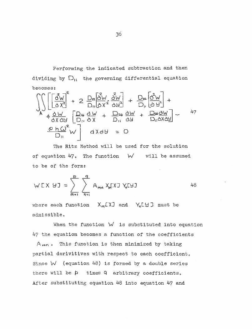
36

Performing the indicated subtraction and then dividing by D lt the governing differential equation becomes:

■r -z -f6 V l \_6 Xj

A 4 6 W£ h G f

D m

+ 2 — nD md W 6 Xno*

|_D„

6 W f 3W_6Xa* ay!;

4 Pqx D„

6aWay' 4

, + _ D ^ a w 1 _ ^7Du ay Dtl6xayJw d X d y - o

The Hitz Method will be used for the solution of equation 47* The function W will be assumed to be of the form:

w c x yu =m* i

Awrt \ f X J XEUJ 48

where each function Xm£XJ and Y„LyD must beadmissible.

When the function W is substituted into equation 47 the equation becomes a function of the coefficients A m n o This function is then minimized by taking

partial derivitives with respect to each coefficient0 Since W (equation 48) is formed by a double series there will be £ times q arbitrary coefficients.After substituting equation 48 into equation 47 and

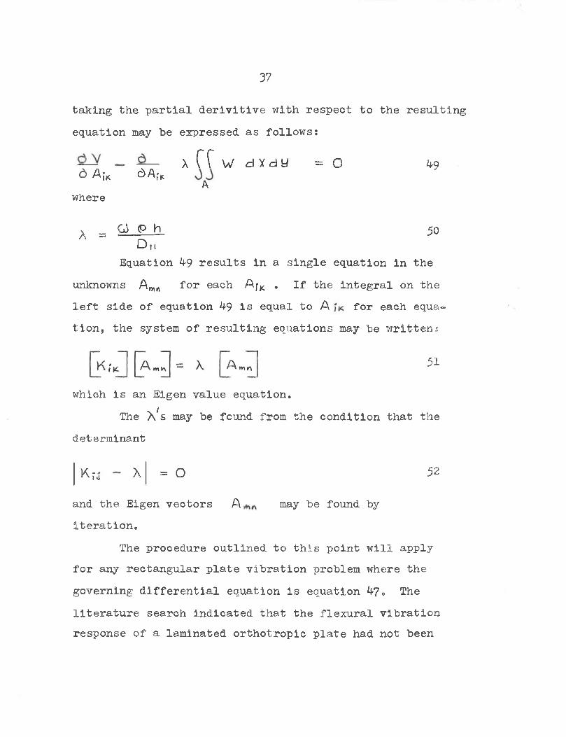
37taking the partial derivitive with respect to the resulting equation may be expressed as follows:

X ( T W d X d y = o 49d A iK 6 A r* Awhere

X = P g-b- 50Dll

Equation 49 results in a single equation in the unknowns A Wrt for each AfK . If the integral on the left side of equation 49 is equal to A for each equa­tion, the system of resulting equations may be written:

which is an Eigen value equation.The X p may be found from the condition that the

determinant

K:wt X = o 52and the Eigen vectors A may be found byiteration.

The procedure outlined to this point will apply for any rectangular plate vibration problem where the governing differential equation is equation 47. The literature search indicated that the flexural vibration response of a laminated orthotropic plate had not been

51

38

analyzed for the case of a cantilevered plate so that solution will be developed in detail.

Detailed Solution for the Frequencies and Mode Shapes of a Cantilevered, Laminated Orthotropic Plate

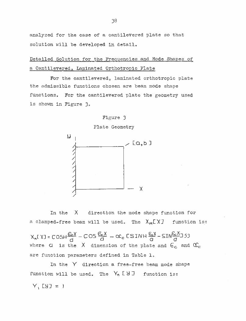
For the cantilevered, laminated orthotropic plate the admissible functions chosen are beam mode shapefunctions. For the cantilevered plate the geometry usedis shown in Figure 3«

Figure 3 Plate Geometry

________ ^ La,bD

— X

In the X direction the mode shape function fora clamped-free beam will be used. The X^CXJ function is:

x„[ TO = COSH--cos -OCcCSINH^- 53where O is the X dimension of the plate and G c and CCc are function parameters defined in Table 1.

In the Y direction a free-free beam mode shape function will be used. The Yn L J function is:

Y, i U J = I

/•///////////

u I

39

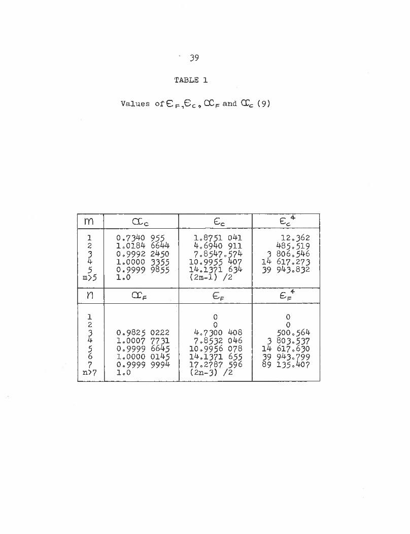
TABLE 1

Values of G P,GC , QCp and QCc (9)

m CCc £c £ 4 °ci 0.7340 955 1.8751 04l 12.3622 lo0l84 6644 4.6940 911 485.5193 0.9992 2450 7c8547.574 3 806.5464 1.0000 3355 10.9955 407 14 617.2735 0.9999 9855 14.1371 634 39 943.832

m>5 1.0 (2m-l) /2n GCF £ P4i 0 02 0 03 0.9825 0222 4.7300 408 500.5644 1.0007 7731 7.8532 046 3 803.5375 0.9999 6645 10.9956 078 14 617.6306 1.0000 0145 14.1371 655 39 943.7997 0.9999 999^ 17.2787 596 89 135.407n>7 1.0 (2n~ 3) /2

40

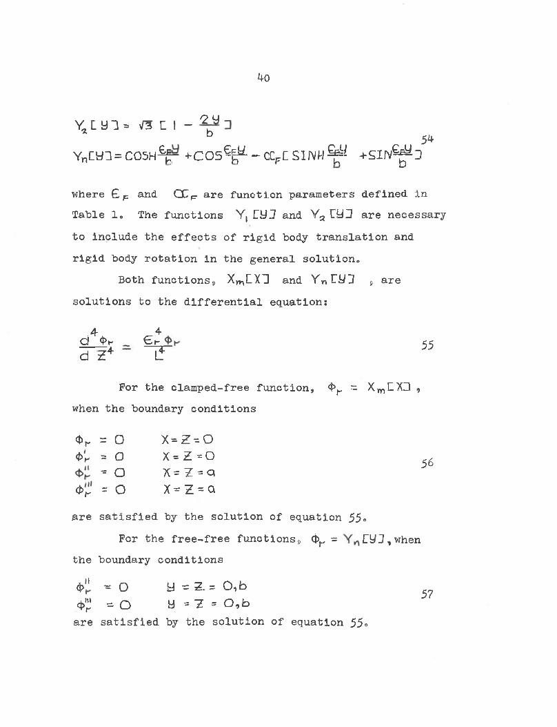
Ya Lyi=: sf3 L \ - 2 y

YnCyi = C05H^- +C05ۤ^-OCfCS1NW%* +SIN^J54

where £ F and CC^ are function parameters defined in Table 1. The functions Y, DJJ and V2 Uyj are necessary to include the effects of rigid body translation and rigid body rotation in the general solution,.

Both functions9 Xm LXTl and YnLUJ 9 are solutions to the differential equation:

d % v d Z+

4Gt-I T 55

For the clamped-free function, <ty = X^LXIl , when the boundary conditions

<*v = O X-Z^OK = O x=z = o

- O X= Z = Q<*V = O X = Z = Qare satisfied by the solution of equation 55„

For the free-free functions9 <j>r = Hyj , when the boundary conditions

4>" * O y = 21= 0,b^ * o y * z » o ,bare satisfied by the solution of equation 55»

57

56

b

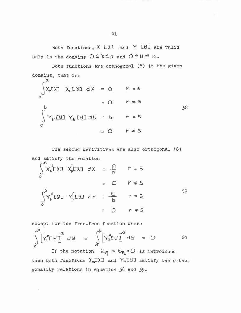
Both functions, X EX1 and V CtJl are valid only In the domains O — X — O and O — y — b,

Both functions are orthogonal (8) in the givendomains, that is:

aXfZXJ XsL X I d X = Q

= O

r rLUJ r s tyj d y = b

= o

K = £

r ^ S

K — £

r ^ S

58

The second derivitives are also orthogonal (8)and satisfy the relation

~o-SX^ZXJ XSLY3 dX = -g -

= ObW^'cyi Y^cyj d y = —o

- o

r - s

r s

r = s

r * S

59

6oexcept for the free-free function where (^° 2 'Z\ [V,llna5] dy -- \ [ v “cy5] dy = oo °

If the notation £p - 0 P = 0 is introducedIthen both functions X^EXl and satisfy the ortho­gonality relations in equation 58 and 59<>

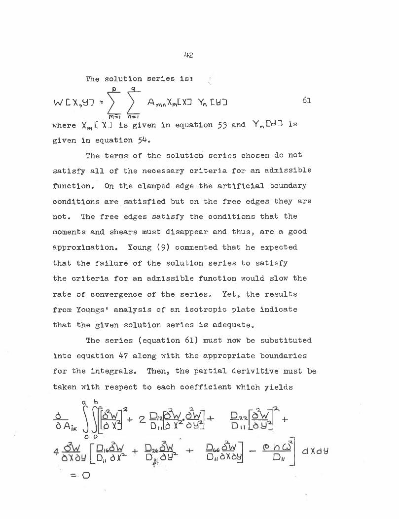
The solution series is:

w c x , y i -m=i n-

A ^ X ^ L X D Yn Eyi 6l

where X^CXH is given in equation 53 and Y^HyD is given in equation 54.

The terms of the solution series chosen do not satisfy all of the necessary criteria for an admissible function. On the clamped edge the artificial boundary conditions are satisfied but on the free edges they are not. The free edges satisfy the conditions that the moments and shears must disappear and thus, are a good approximation. Young (9) commented that he expected that the failure of the solution series to satisfy the criteria for an admissible function would slow the rate of convergence of the series. Yet, the results from Youngs' analysis of an isotropic plate indicate that the given solution series is adequate.

The series (equation 6l) must now be substituted into equation 47 along with the appropriate boundaries for the integrals. Then, the partial derivitive must be taken with respect to each coefficient which yields

a b±=Ln-2. £>W

r a

0 o

D „ 6 f D „ d y ^l— 1 jjjn.-;

^ O

4-

kz

A3

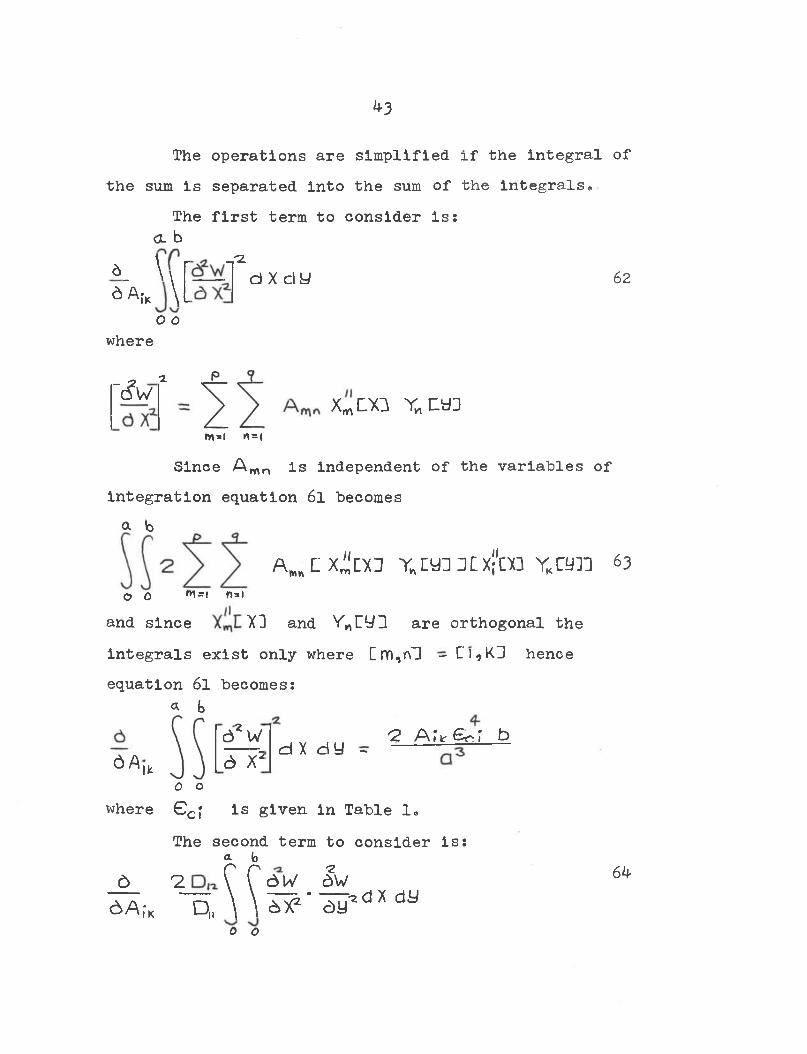
The operations are simplified if the integral of the sum is separated into the sum of the Integrals,

The first term to consider is:a b

6. 1v rd AfK Vo 0where

~C?W■z

-T2.d x ciy 62

X^LX3 Y^LyDrw=l rt = |

Since A mn is independent of the variables of Integration equation 6l becomes a b

il.A ^ C X ^ D O Y^CyiJCX;ra YKry]l 63o o 01=1 n=i

and since X3 and Y^CyH are orthogonal theintegrals exist only where Cm,nil - U),KD hence equation 6l becomes:

« b

6 A I k

d 2 W d X2

<2 A ^ e ^ r b<d X d y ~ --- ------O o

where G cj is given in Table 1.The second term to consider is:

a. fa

6 Z C f div <?W^,-K ^ \ W ‘ ^ d X d a

64

0 o

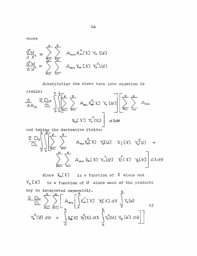
44

where

<fw _6 X'2- 62W _6 ya

A mnxilrXD Y. Ey3

A mn x* lx: yJ'w i

Substituting the above term into equation 64 yields: a .6 2 D(iAj^ D|,

iia^ xjixd y„ ry:

X^LXD Yn I50

S i-rn-i n=i

dxdy

and taking the derivative yields:OL #2 D ,D,

n\

6 o

A„„>c!rx] Y„cyj K;txi Yjy] •+wwi O-i

A m *xmLx: y^ luj xf'nx: YtLy:m-i nm

d X d y

Since X CXl is a function of X alone and Y^LyU is a function of fc/ alone each of the productsmay be integrated separately.

^ f f f AD„ / / A "*Ol-ai r ( 1L 0

Xwtx: X]Lxi dx \ Yjyifa

yScm dy + ^xj;w xfoa dx W ty j yk an dy

6 5

45

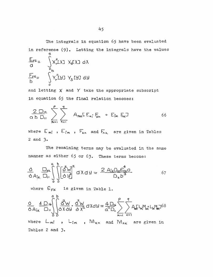
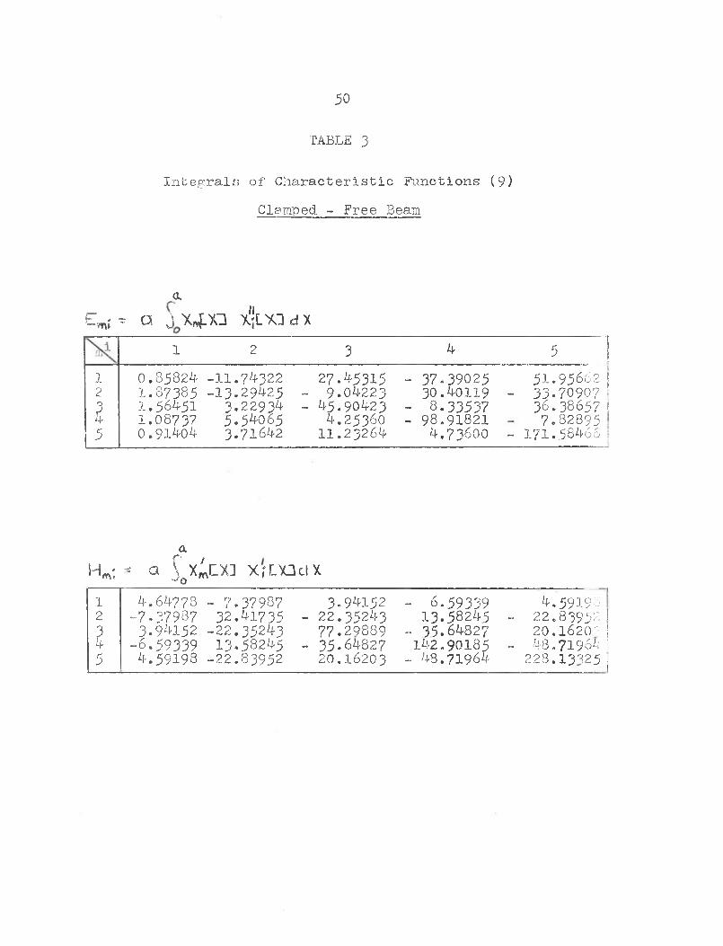
The integrals in equation 65 have been evaluatedin reference (9). Letting the integrals have the values

a.

-|rs= \x|ix3 xsm dX°b^ Y K*ta3 vs ca: dy0

and letting X and Y take the appropriate subscript in equation 65 the final relation becomes:

2 D m. q b Du

rvi— t ft-1A MnL E • Fu L-mi V* •l*ft 66

where E m; , D,*,* , and Fv^ are given in Tables2 and 3«

The remaining terms may be evaluated in the same manner as either 65 or 63. These terms become:

a b r- 2. —a6 W6 a 2 d X d y = - D (lb' 67

O Owhere G FK

a bis given in Table 1,

6_6 A jk,

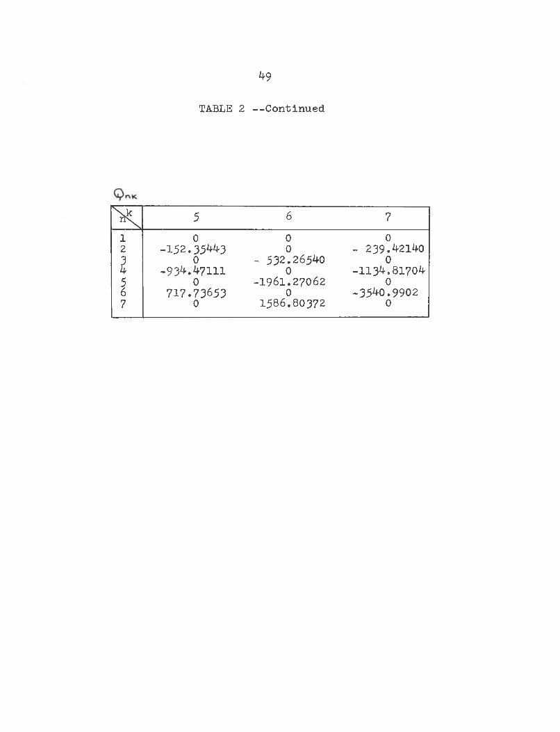
o O rvi=.| ft - >where , Lj^ , IV1 ^ and FV)nfc are given inTables 2 and 3»

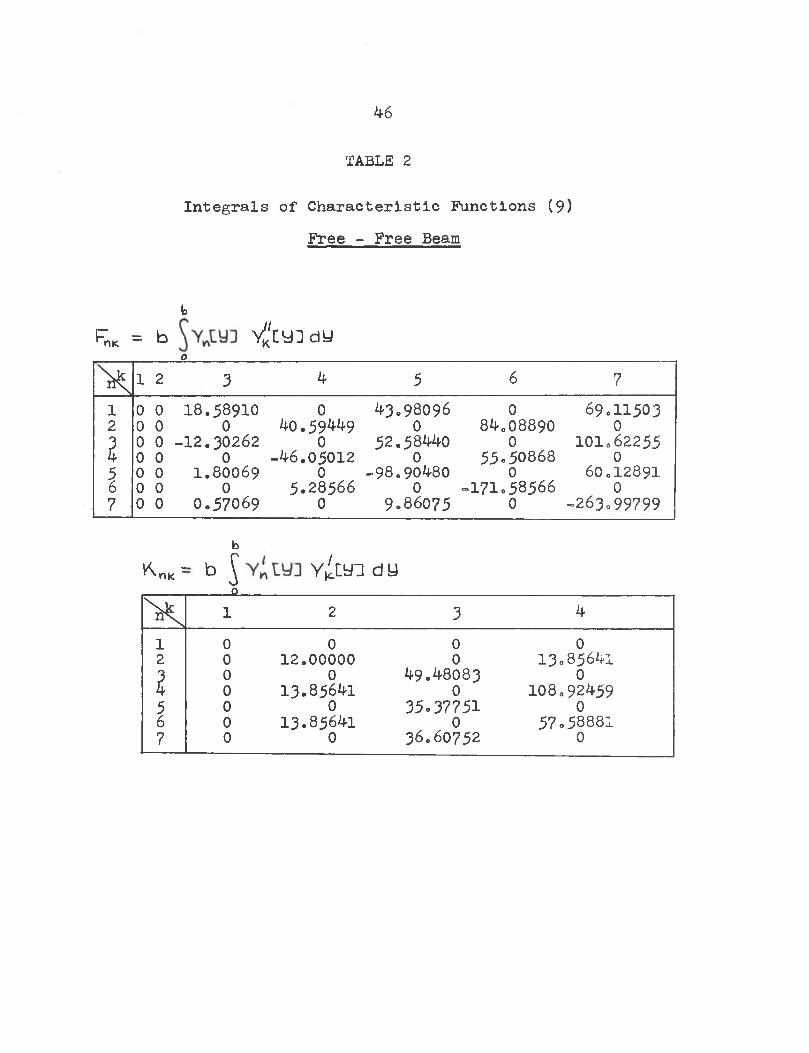
TABLE 2

Integrals of Characteristic Functions (9) Free - Free Beam

kFnK = b V^cyDdy

oX 1 2 3 4 5 6 71 0 0 18.58910 0 43.98096 0 69.115032 0 0 0 40.59449 0 84.08890 03 0 0 -12.30262 0 52.58440 0 101.622554 0 0 0 -46.05012 0 55.50868 05 0 0 1.80069 0 -98.90480 0 60.128916 0 0 0 5.28566 0 -171.58566 07 0 0 0.57069 0 9.86075 0 -263.99799

bV W X0

y^cyi d y

X 1 2 3 41 0 0 0 02 0 12.00000 0 13.856413 0 0 49.48083 04 0 13.85641 0 108.924595 0 0 35.37751 06 0 13.85641 0 57.588817 0 0 36.60752 0

46

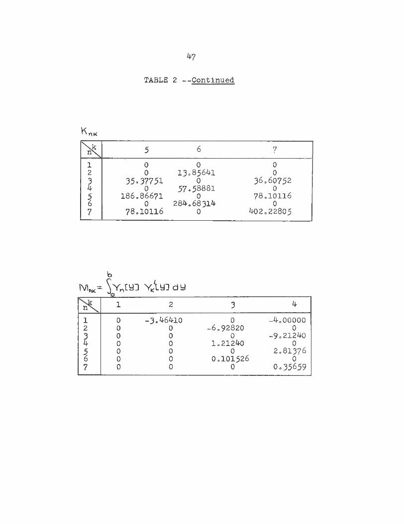
TABLE 2 --Continued

X 5 6 71 0 0 02 0 13.85641 03 35° 37751 0 36.607524 0 57°5888l 05 186.86671 0 78.101166 0 284.68314 07 78.10116 0 402.22805

bNi^= ^ Y ntyi Y^iyi d y

n^\ 1 2 3 41 0 -3.46410 0 -4.000002 0 0 -6.92820 03 0 0 0 -9.212404 0 0 1.21240 05 0 0 0 2.813766 0 0 0.101526 07 0 0 0 0.35659

K„«

b9*k= S y . dd Y “ cyj dy

o

MnK

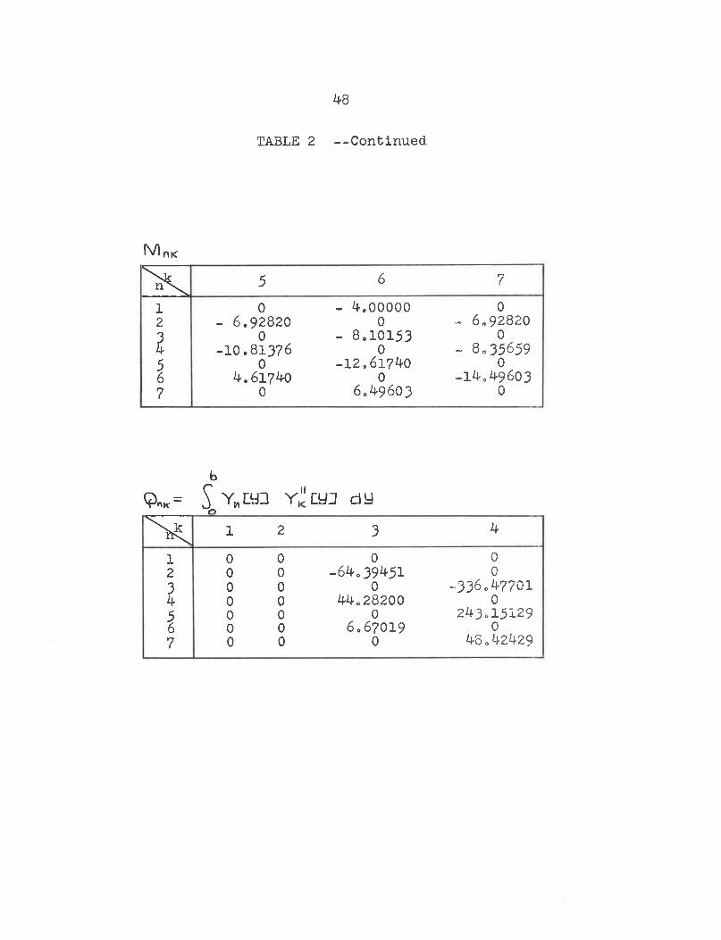
TABLE 2 --Continued.

48

X 5 6 71 0 - 4.00000 02 - 6.92820 0 - 6.928203 0 - 8.10153 04 -10.81376 0 - 8.356595 0 -12,61740 06 4.61740 0 -14.496037 0 6.49603 0

X 1 2 3 4

1 0 0 0 02 0 0 -64,39451 03 0 0 0 -336.477014 0 0 44.28200 05 0 0 0 243.151296 0 0 6.67019 07 0 0 0 48,42429

49

TABLE 2 — Continued

X 5 6 71 0 0 02 -152.35^3 0 - 239.421403 0 - 532.26540 04 -93^7111 0 -1134.817045 0 -1961.27062 06 717.73653 0 -3540.99027 0 1586.80372 0

50

TABLE 3

Integrals of Characteristic Functions (9)Clamped. - Free Beam

a.ew ■= a j x„pa x'jixi d x

l 2 3 4 5 11 0.85824 -11.74322 27.45315 - 37.39025 51.95662 |2 1.87385 -13.29425 - 9.04223 30.40119 - 33.70907 '3 1.56451 3.22934 - 45.90423 - 8.33537 36.38657 14 1.08737 5.54065 4.25360 - 98.91821 7.828955 0.91404 3.71642 11.23264 4.73600 - 171.58466

aHm; = a ^ C X ] XrDQclX1 4.64778 - 7.37987 3.94152 - 6.59339 4.591982 -7.3798? 32.41735 - 22.35243 13.58245 - 22.839522 3.94152 -22.35243 77.29889 ~ 35.64827 20.16203

-6.59339 13.58245 - 35.64827 142.90185 - 48.719665 4.59198 -22.83952 20.16203 - 48.71964 228.13325

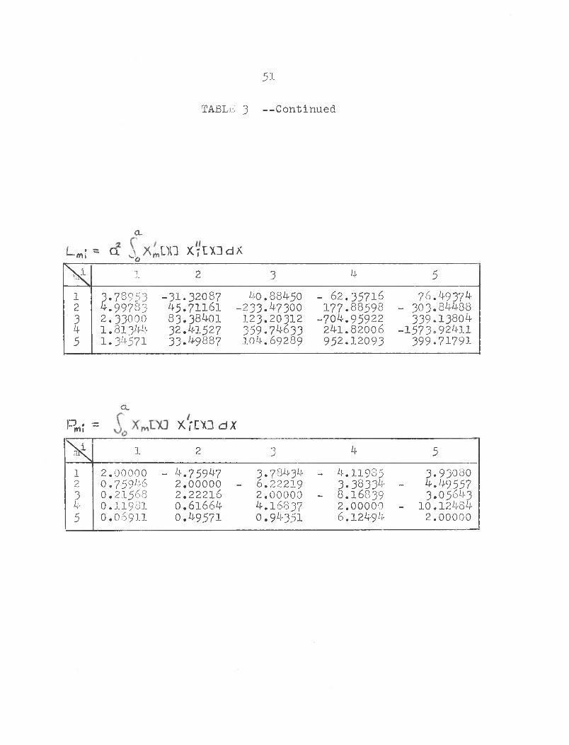
51

TABLE 3 --Continued

aLm; - CL j X*DG XrtXDdX_____ O __X 1 2 3 4 51 3.78953 -31.32087 40.88450 - 62.35716 76.493742 4.99783 45.71161 -233.47300 177.88598 - 303.844883 2.33000 83.38401 123.20312 -704.95922 339.138044 I.8I3EE 32.41527 359.74633 241.82006 -1573.924115 1.3 -571 33.49887 104.69289 952.12093 399.71791

CL

Pm; = XfEXBdXX 1 2 3 4 51 2.00000 - 4.75947 3.78434 - 4.11985 3.930802 0.75946 2.00000 - 6.22219 3.38334 - 4.495573 0.21568 2.22216 2.00000 - 8.16839 3.056434 0.11981 0.61664 4.16837 2.00000 - 10.124845 O.O69II 0.49571 0.94351 6.12494 2.00000

52

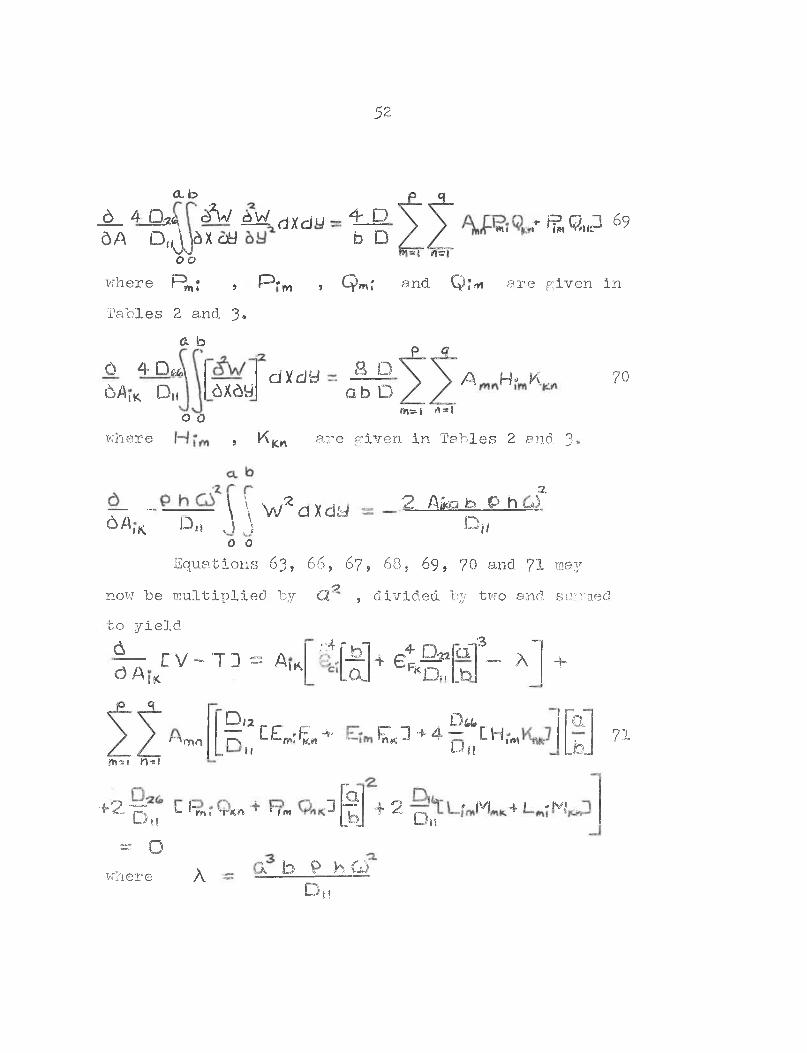
a . b<5 4-O A c^W cb W (-j % d lj A - D5A D (,jjaxcfcl b D

oorfcQ„P 69mi m

where F^,j , P « m , Q w ; and Q;*t are given in

Tables 2 and 3®C. b

0 4* D fy&$ ik Du 6X6y axciy -8 D

o b D /A. H 13 /Ao o m=-i «*•

where , K Kw are given in Tables 2 and 3*

70

— ••• — — \ \ W 2 d X duDu „1 .)■s.

6AiK2 A lka b P h u )

D „0 0

Equations 63, 66, 6 7 , 68, 6 9 , 70 and 71 mayspnow be multiplied by <2 , divided by two and summed

bo yielddd A C V - T 3 = A I K

I K

' ;-4 r bi.OL > e ^ 2On

__3 - 1Cl - A_b

n mn ms* *1«*

+ 2,"^ *- I'mD t|= O

where A

D/a DfctO C £*••: t w ** £« 3 •+ 4 — LH «■*». ! I Ult71

mi 'rKn ' 'fro 1 D # jv/ 4 I «IVjit

k to P H G)D I!

-f

"d_b_

rGtT- + 2!>J

53

For each A equation 71 yields one equation in terms of A mn . This expansion yields an Eigen value equation of the type described by equation 51.

Equation 71 was expanded for the case P = 3 and <? = G . The coefficients were determined leaving the stiffness ratios and length to breadth ratio undetermined. The resulting equations were programed in Fortran IV (11) and adapted for use in an IBM 7040 digital computer.The computer program and its usage are discussed in Appendix A. The analytical results derived from equation 71 will be discussed in Chapter V.

CHAPTER V

ANALYTICAL AND EXPERIMENTAL RESULTS

The analysis presented to this point is valid for any laminate which is composed of laminae of an ortho­tropic material with the laminae oriented pairwise about the middle surface of the laminate. The pairwise orien­tation is to assure elastic symmetry about the middle surface. The pairwise symmetry uncouples bending and tension effects and thus, if the laminate is to be sub­jected to bending forces, the laminae must not only be pairwise oriented but must also possess identical properties in tension and compression. The laminate needed for the experimental verification of this analysis should be composed of layers of an orthotropic material which has equal tension and compression properties and has all layers oriented with pairwise symmetry about the middle surface of the laminate.

(r)The material used for this study was Scotchply1 type 1002, parallel glass filament reinforced plastic which is manufactured by Minnesota Mining and Manu-

(Dfacturing Company. The elastic properties of Scotchply^ type 1002 have been extensively investigated by Davis

and Zurkowski (12)

55

The Static Properties of Sootchply® Type 1002Equations 21 and 23 predict that the in-plane

and flexural behavior of a laminate composed of ortho­tropic laminae may be determined if the elastic properties of each layer are known.

For an orthotropic lamina the independent elastic properties are E, , E^ , kJ| , and G . E, ,E-2. and U| may all be determined from simple tension tests. E, will be defined as the modulus of elasticity measured parallel to the filament direction in a laminae, E ^ is the modulus measured perpendicular to the filament direction and KJ( is the Poisson's ratio determined by the ratio of the strain perpendicular to the filament direction divided by the strain parallel to the filament direction.It is obvious that E , , E a and may be determinedfrom the elastic properties of a unidirectional laminate.

The data obtained by Davis and Zurkowskl (12) may be verified analytically. They ran three primary tests which are of interest. The first tests determined the modulus of elasticity in tension for an eleven ply laminate with the principle layers alternating at 0°,+15°, +30°, +60°, +75° and 90°. Then, the modulus of elasticity in compression and the apparent flexural modulus of elasticity was determined for the same layer configurations. The eleven ply laminate insures that the

56

tension and flexure properties are uncoupled, ( i f t h e

modulus of elasticity is the same in tension a n d

compression or the laminate is subjected to t e n s i o n o r

compression loads only) however, the laminate i s s l i g h t l y

anisotropic in both tensile and flexural loads. Because the number of layers is high the tensile anisotropy may be ignored and it is possible to gain some valid modulus data from these tests,

Davis and Zurkowski determined that the apparent modulus of elasticity for all of the above mentioned lamina configurations was different for tension and compression loads. If this is true then the apparent flexural modulus could be calculated from the tension and compression modulus.

The flexural modulus of elasticity was determined by subjecting a beam constructed from the laminate to a concentrated load placed midway between simply supported edges. The deflection of the beam may be related to an apparent modulus by the relation

e ,ppi J-J = m mwhere ET^pp is the apparent modulus, I is the first area moment of the beam section, y is the deflection and M L X 1 is the applied moment as a function of X position on the beam. For a simply supported beam with a

57

centrally placed concentrated load the apparent mod as

in terms of the deflection at the load becomes,

48 y iwhere P is the load, I— is the length of the beam,

*

y the deflection at the load, and I the first area moment of the beam section. These calculations yield an apparent flexural modulus for the beam.

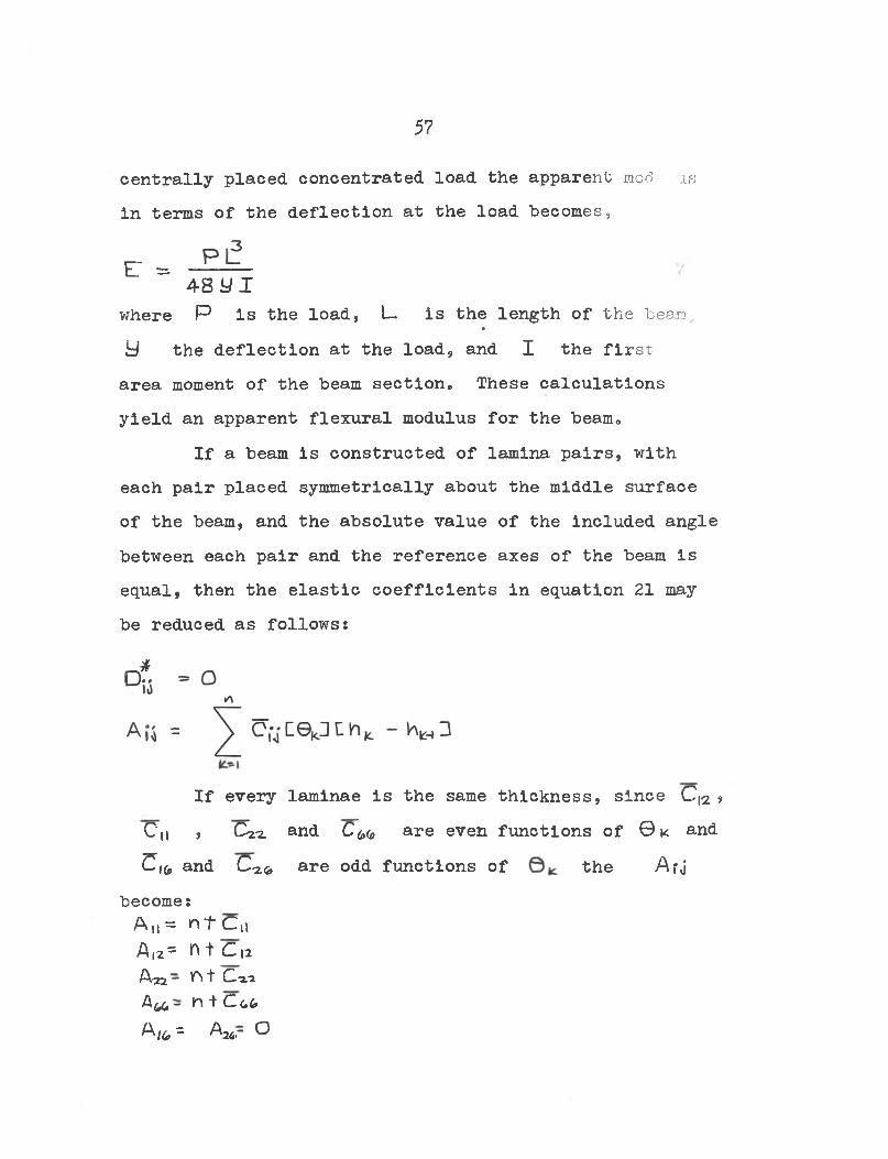
If a beam is constructed of lamina pairs, with each pair placed symmetrically about the middle surface of the beam, and the absolute value of the included angle between each pair and the reference axes of the beam is equal, then the elastic coefficients in equation 21 may be reduced as follows:

If every laminae is the same thickness, since C )2 > C„ , C-2-2. and are even functions of © « and

A„= nt C u A,2* H t C|2 Ao2~ ^ t C.-2.2 Am- mi Cc.£, A * - A*r O

e: =

and C -26 are odd functions of the Arjbecome:

C m are^ I0>

where Y\ is the number of layers and "t thicknesses.

the layer

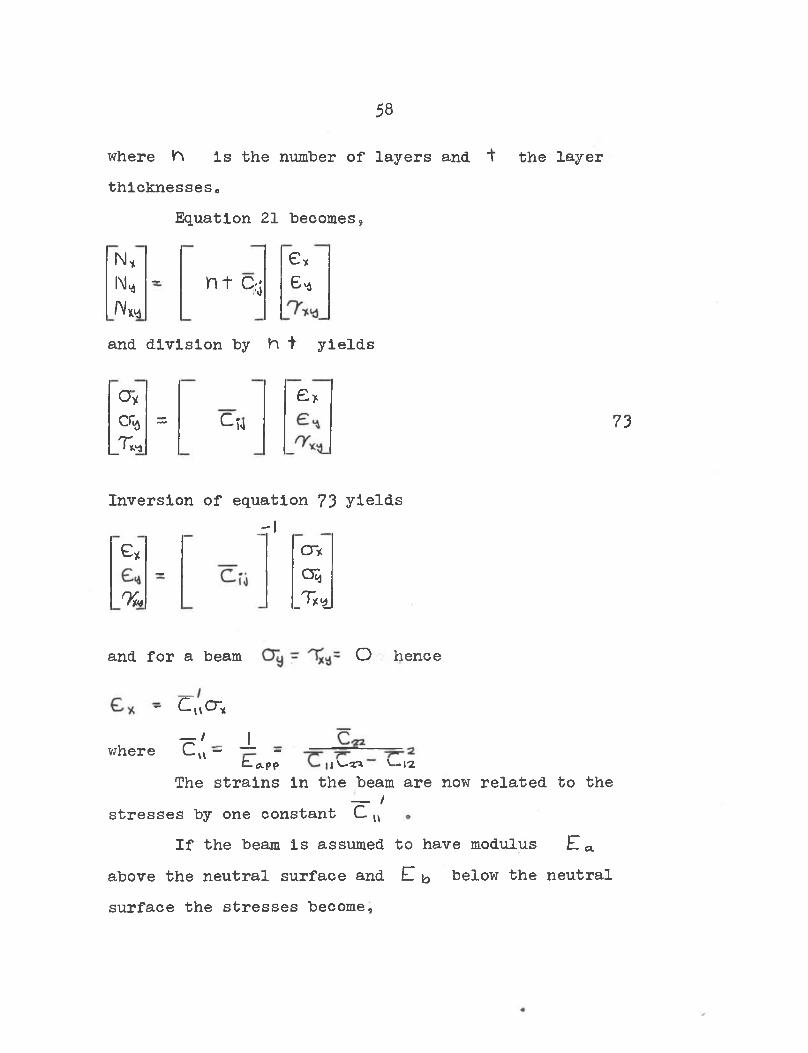
Equation 21 becomes,

N* e*IM* ~ n + P s e*N**and division by h + yields

Oy £ rcr* = Ci4

_r«73

Inversion of equation 73 yields_rlGy cr*

- cry% _T*iand for a beam O hence

~ C,vcr,7=:7 _ Iwhere L-u — — -t-cLpp 11'—-ar» U-C2The strains in the beam are now related to the

— /stresses by one constant C uIf the beam is assumed to have modulus E a

above the neutral surface and E below the neutral surface the stresses become9

58

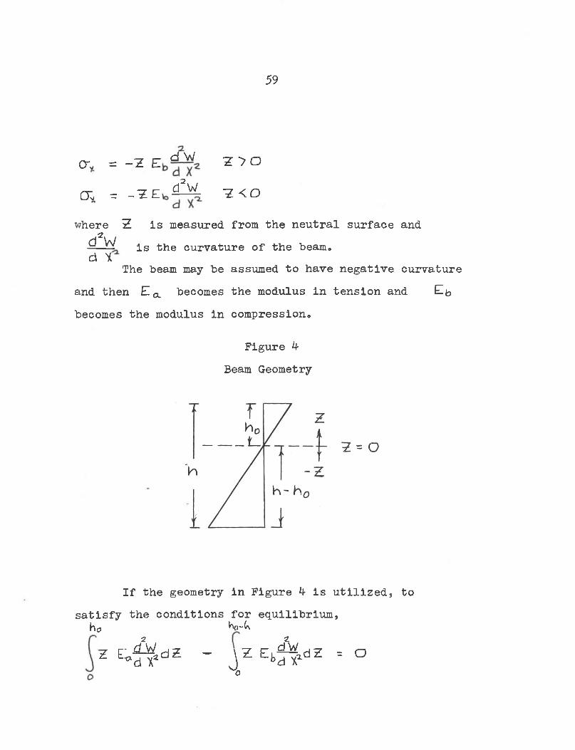
59

Crv = ~Z E(X = -IE

d Wd2W z <o

where Z is measured from the neutral surface and is the curvature of the beam*d*W

d tThe beam may be assumed to have negative curvature

and then E a becomes the modulus in tension and Eb becomes the modulus in compression*

Figure 4 Beam Geometry

If the geometry in Figure b is utilized, tosatisfy the conditions for equilibrium,

h0 h<>-C\Z E ^ d E - J z EA dz - °

Vs'0

D O

60

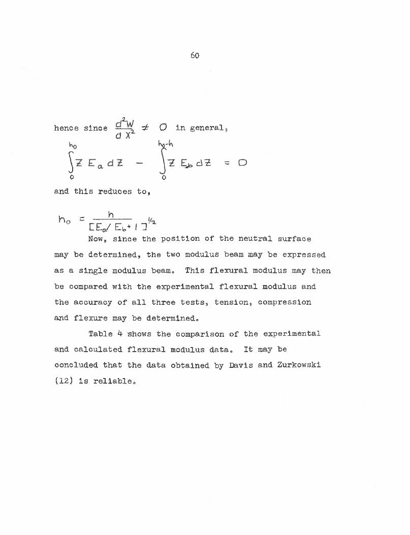
.Z\ihence since ^ O in general,

d

5 -o o

and. this reduces to,

h 0 c hZ Z J Eu+ I 1 ‘

Now, since the position of the neutral surface may be determined, the two modulus beam may be expressed as a single modulus beam. This flexural modulus may then be compared with the experimental flexural modulus and the accuracy of all three tests, tension, compression and flexure may be determined.

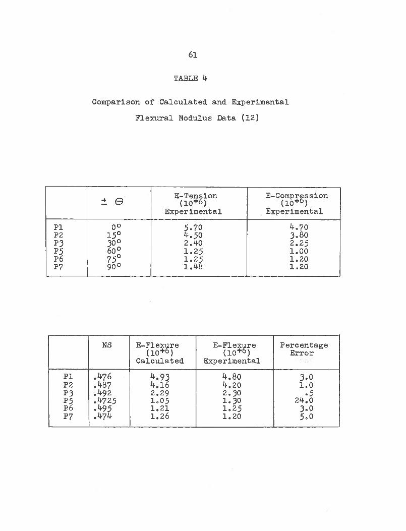
Table k shows the comparison of the experimental and calculated flexural modulus data. It may be concluded that the data obtained by Davis and Zurkowski (12) is reliable.

6l

TABLE 4

Comparison of Calculated and Experimental Flexural Modulus Data (12)

± © E-Tension (10*°) Experimental

E-Compression(10+g)Experimental

PI 0° 5.70 4.70P2 15° 4.50 3.80P3 30° 2.40 2.25P5 60° 1.25 1.00P6 75° 1.25 1.20P7 90° 1.48 1.20

NS E-Flexure (10+5) Calculated

E-Flexure (10+5) Experimental

PercentageError

PI .476 4.93 4.80 3.0P2 .487 4.16 4.20 1.0P3 .492 2.29 2.30 .5P5 .4725 1.05 1.30 24.0P6 .495 1.21 1.25 3.0P7 ,4?4 1.26 1.20 5 o0

62

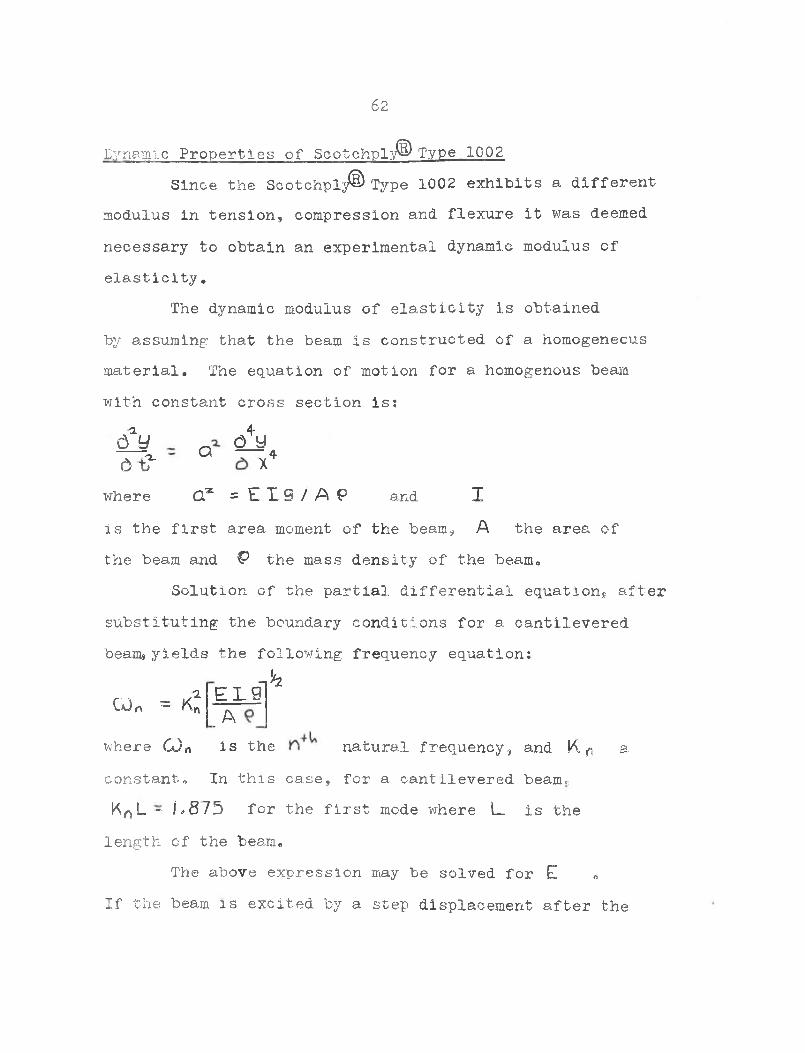
Dynamic Properties of Scotchpl:,® Type 1002Since the Scotchply® Type 1002 exhibits a different

modulus in tension, compression and flexure it was deemed

necessary to obtain an experimental dynamic modulus of

elasticity.

The dynamic modulus of elasticity is obtained

by assuming that the beam is constructed of a homogeneous

material. The equation of motion for a homogenous beam

with constant cross section is;

d^y6 t?"

4-6 yQ 4

X

where a * = E I S / A P and I

is the first area moment of the beam, A the area of

the beam and P the mass density of the beam.

Solution of the partial differential equations after

substituting the boundary conditions for a cantilevered

beam, yields the following frequency equation;

-AE 1 9 . A

where O n is the natural frequency, and K a

constant. In this case, for a cantilevered beam-.,

K r> L » L875 for the first mode where L_ is the

length of the beam.

The above expression may be solved for E .

If the beam is excited by a step displacement after the

CO. = kI

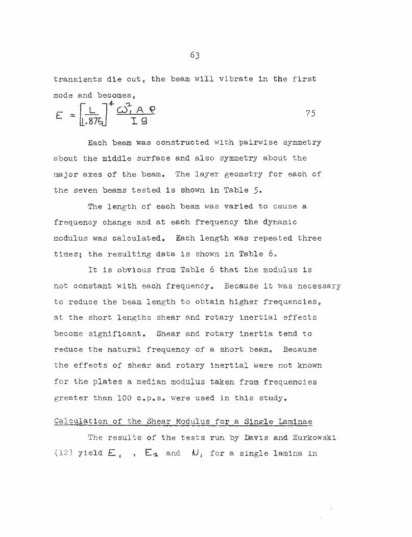
63

transients die out, the beam will vibrate in the first mode and becomes,

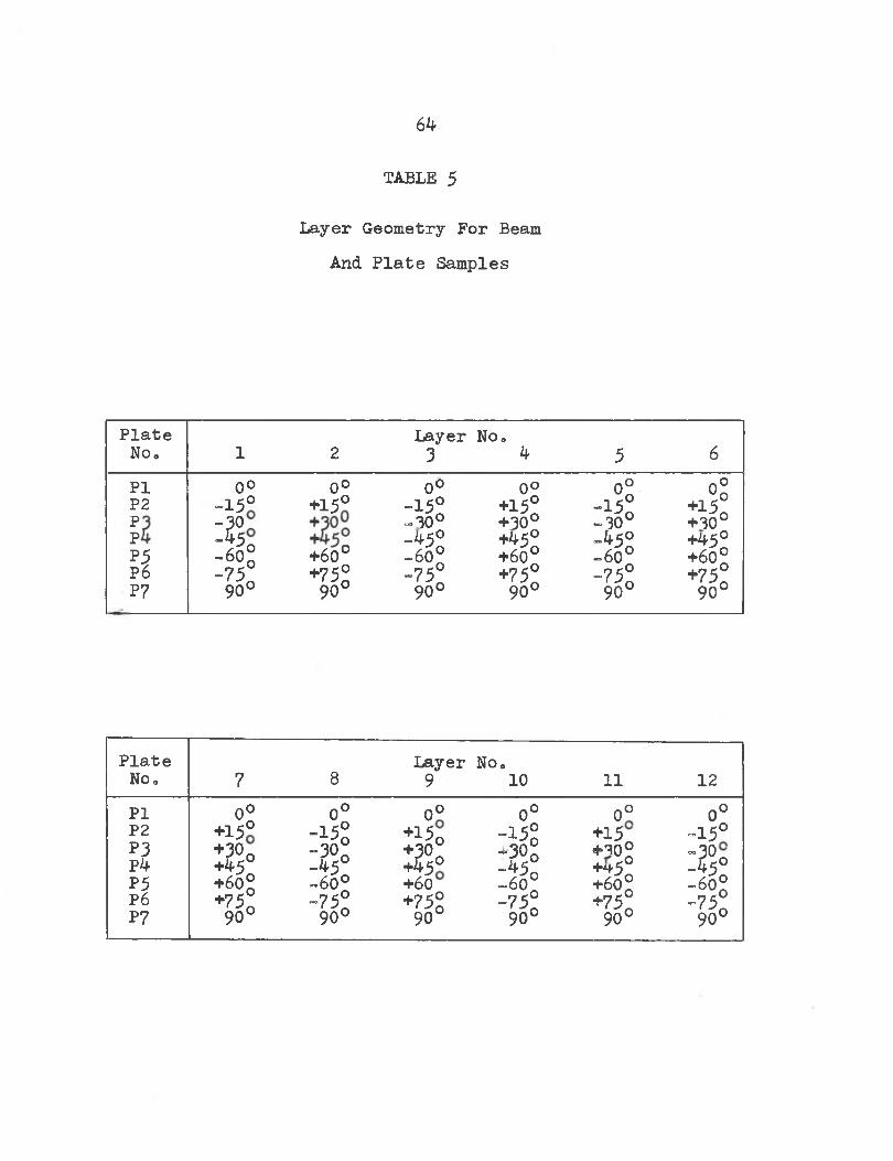
Each beam was constructed with pairwise symmetry about the middle surface and also symmetry about the major axes of the beam. The layer geometry for each of the seven beams tested is shown in Table 5»

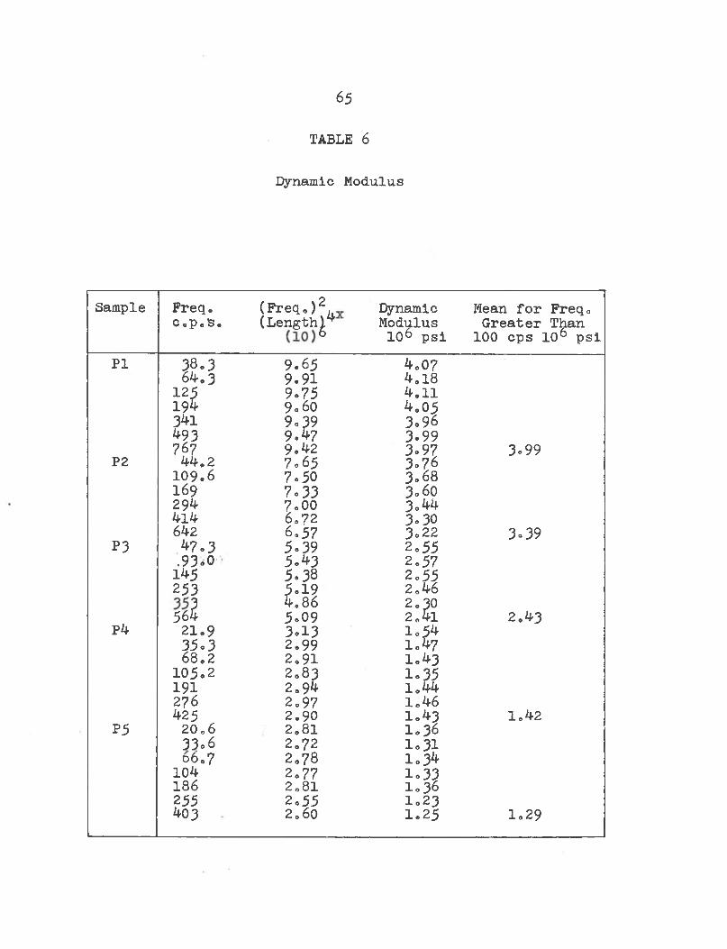
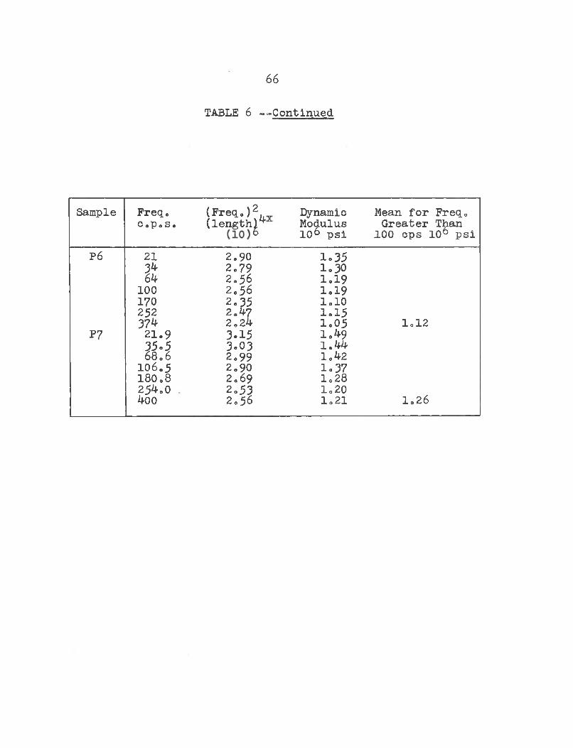
The length of each beam was varied to cause a frequency change and at each frequency the dynamic modulus was calculated. Each length was repeated three times; the resulting data is shown in Table 6.

It is obvious from Table 6 that the modulus is not constant with each frequency. Because it was necessary to reduce the beam length to obtain higher frequencies, at the short lengths shear and rotary Inertial effects become significant. Shear and rotary Inertia tend to reduce the natural frequency of a short beam. Because the effects of shear and rotary inertial were not known for the plates a median modulus taken from frequencies greater than 100 c.p.s. were used in this study.

Calculation of the Shear Modulus for a Single LaminaeThe results of the tests run by Davis and Zurkowski

(12) yield EL, , Ei and U, for a single lamina in

75

64

TABLE 5

Layer Geometry For Beam And Plate Samples

PlateNo. 1 2

Layer No»3 4 5 6

PI 0° 0° 0° 0° 0° 0°P2 -15° +15° -15° +15° -15° +15°1 I :205 -30°

-45°+30°+45°

-30°-45°

+30°+45°P 5 -60° +60° -60° +60° -60° +60°P6 -75° +75° -75° +75° -75° +75°P7 90° 90° 90° 90° 90° 90°

Plate Layer No.No. 7 8 9 10 11 12PI 0° 0° 0° 0° 0° 0°P2 +15° -15° +15o -15S +15 -15°P3P4 +30o

+45-30°.45° +30°

+^5° *30°-45°+30°++5° •J°5 °P5 +60° -60° +6o -60° +6o° “60°P6 +75° —7 5° +75° -75° +75° -75°P7 90° 90° 90° 90° 90° 90°

65

TABLE 6

Dynam ic M odulus

Sample Freq. (Freq.)2.(Length^

Dynamic Mean for Freq.c.p.s. Modulus 106 psi Greater Than 100 cps 106 psi

PI 3?*3 9*65 4.0764.3 9*91 4.18125 9*75 4.11194 9*60 4.053^1 9*39 3*96493 9*47 3*99767 9*42 3*97 3*99P2 44.2 7*65 3-76109.6 7*50 3*68169 7*33 3*60294 7*00 3*44414 6.72 3*30642 6.57 3.22 3*39P3 47.3 5*39 2*55.93*0 5*43 2*57145 5*38 2*55253 5*19 2.46

P4 56^ 4.865*09

2.302.41 2.4321.9 3*13 1.5435*3 2*99 1*4768.2 2.91 1.43

105*2 2.83 1.35191 2.94 1.44276 2*97 1.46425 2.90 1.43 1.42p 5 20.6 2.81 1*36

33.6 2.72 1*3106.7 2.78 1.34104 2*77 1*33186 2.81 1.36255 2*55 1.23403 2.60 I.25 1.29

66

TABLE 6 --C o n tin u ed

Sample Freq.Cop®S«

(Freq.)2.(length^

Dynamic Modulus 106 psi

Mean for Freq.Greater Than 100 ops 10° psi

P6 21 2.90 lo353^ 2.79 1.306k 2.56 1.19100 2.56 1.19170 2.35 1.10252 2.47 1.15y?k 2.24 1.05 1.12

P 7 21.9 3.15 1.4935»5 3.03 1.4468.6 2.99 1.42

IO6.5 2.90 1.37180.8 2.69 1.28254.0 2o53 1.20400 2.56 1.21 1.26

67

te n s io n and com pression,. Then d ata a l s o y i e l d s an

e q u iv a le n t modulus fo r a la m in a te in f l e x u r e „

The dynamic modulus t e s t s y ie ld e d E, and E 2 fo r a la m in a te b e in g e x c i t e d dynam ically ,,

I f M. i s assumed to n ot change fo r f le x u r e

and dynamic t e s t s i t i s p o s s ib le to c a lc u la t e G , but f i r s t some major assu m p tion s must be made.

At th e f i r s t o f t h i s Chapter i t was n o ted th a t

i f s in g le la y e r p r o p e r t ie s are known i t i s p o s s ib le to

c a lc u la t e th e g r o ss p r o p e r t ie s o f th e la m in a te . T h is

in v o lv e d th e assum ption th a t th e t e n s io n and com press

s io n p r o p e r t ie s fo r a s in g le lam inae are e q u a l. From th e

t e s t r e s u l t s i t was determ ined th a t t h i s i s n o t true,,

th e t e n s io n and com pression p r o p e r t ie s are n o t e q u a l.

The a n a ly s is d eve lop ed to t h i s p o in t i s n o t adequate

to a n a ly z e a la m in a te which i s n o t sym m etric about th e

m iddle s u r fa c e , and th e d i f f e r in g t e n s io n and com pression

p r o p e r t ie s w i l l d e str o y th e symmetry about th e m iddle

s u r fa c e .

To accou n t fo r th e d i f f e r in g p r o p e r t ie s , th r e e

s e t s o f modulus d a ta w i l l be u sed . The f i r s t s e t w i l l

u s e , fo r each la y e r in th e la m in a te , th e E, , and

m i determ ined by t e n s io n t e s t d a ta determ ined from

u n id ir e c t io n a l la m in a te s . Then, from th e d ata o b ta in ed

from sym m etric, o b liq u e a n g le la m in a te s a s in g le la y e r

68

shear modulus will be determined. The second set will utilize the ET, and EI^ determined from flexure tests on unidirectional laminates and jj, from tension tests; from flexure tests performed on symmetric oblique angle laminates the shear modulus will be determined. The third set of data will utilize the E7, and ET^ determined from dynamic response tests, Mi from tension tests, and then the shear modulus will be determined from oblique angle dynamic modulus tests.

Prom equation 73 it is known that if a laminate is composed of alternating layers of the same positive and negative angle, with each layer symmetrically placed about the middle surface the stresses in terms of the strains may be written as follows;

o;0« V“'IJ

Inversion of the above equation and substitution of the stress conditions for a beam 0 ~ 0 D yields,

_____ 0 -3-a. — ___ IC C - ET cr'-'U '-'txFrom equation 13 the C*^ are known and

defining,

Kl - C h C o & Q •+ C,2S tff©Cos © •+• C^xS'toB Y\Z = CiiS i n4© 2 C|45in29Cos20 + C.2z.Co&%K3 - C C m + C^D © U 2© C o *© + C.* LSi/e^Co/©D

69

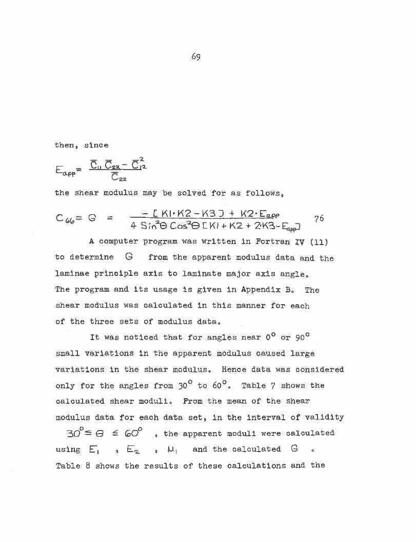
th e n , s in c e

r~ _ C \ \ C-za ~ C i-a.'-app p

th e sh ear modulus may be so lv e d fo r a s f o l lo w s ,

G = - C KI-K2-K3D 4 K2-ET0i4£P 054 S 1 n © Cos2© L K) + K2. + 2"K3-

A computer program was w r it t e n in F ortran IV (11)

to determine G from the apparent modulus data and thelam in ae p r in c ip le a x is to la m in a te major a x i s a n g le .

The program and i t s u sage i s g iv e n in Appendix B, The

sh ear modulus was c a lc u la t e d in t h i s manner fo r each

o f th e th r e e s e t s o f modulus d a ta .

I t was n o t ic e d th a t fo r a n g le s near 0 ° or 90°

sm all v a r ia t io n s in th e apparent modulus caused la r g e

v a r ia t io n s in th e sh ear m odulus. Hence d ata was co n sid er ed

only for the angles from 30° to 60°. Table 7 shows thec a lc u la te d sh ear m od u li. From th e mean o f th e shear

modulus d ata fo r each d a ta s e t , in th e in t e r v a l o f v a l i d i t y o o30 — 0 — GO , the apparent moduli were calculated

using ET, , ET-2 U, and th e c a lc u la te d GT able 8 shows th e r e s u l t s o f th e s e c a lc u la t io n s and th e

o5

70

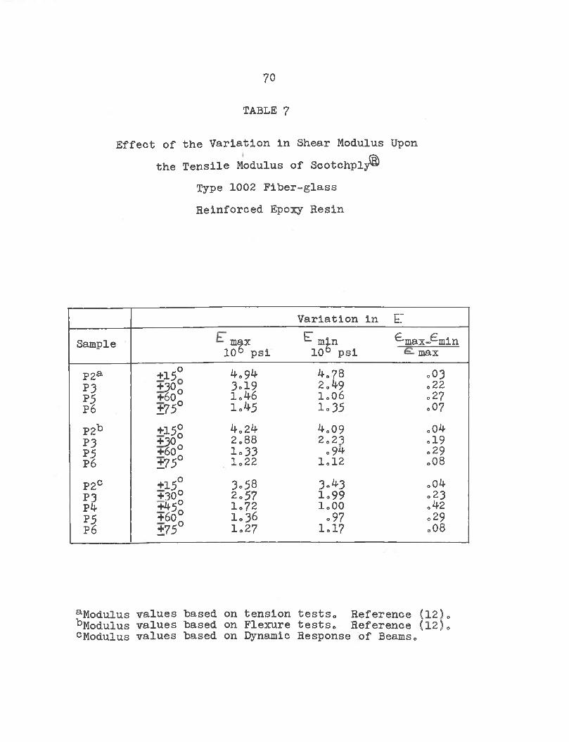
TABLE 7

Effect of the Variation in Shear Modulus Upon the Tensile Modulus of Scotchply®

Type 1002 Fiber-glass Reinforced Epoxy Resin

Variation in e:Sample m^x E min ^•max-^min

10° psi 106 psi maxP2a +15° 4.94 4.78 .03P3 +30 o 3-19 2.49 .22P5 +6,0° 1.46 1.06 ■ 27p 6 ±75° 1.45 1°35 .07P2b +15% 4.24 4.09 .04P3 +30° 2.88 2.23 .19P5 +6o° lo33 .9+ .29P6 ±75° 1.22 1.12 .08p2c +15° 3.58 3»^3 .04P3 +30° 2.57 lo99 .23P4 « 5 ° 1.72 1.00 .42P 5 P 6

+60°±75°

1.36I.27 o97

1.17o29.08

aModulus values based on tension tests. Reference (12)„ ^Modulus values based on Flexure tests. Reference (12)» cModulus values based on Dynamic Response of Beams.

71

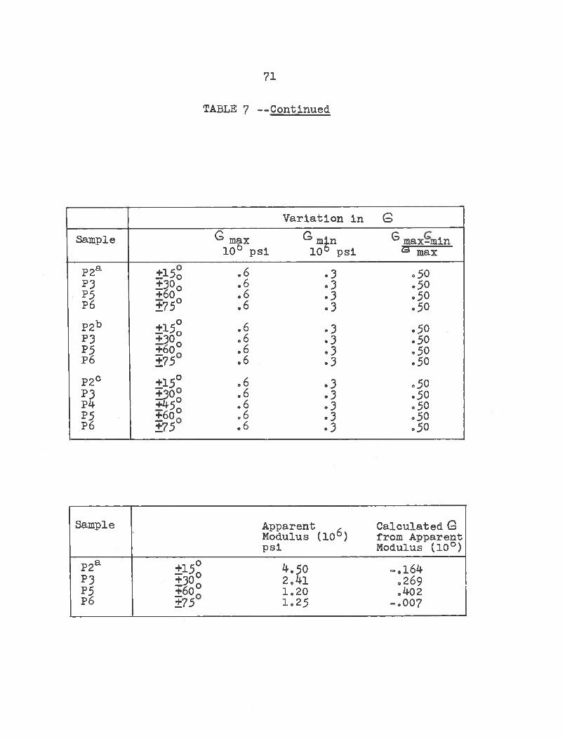
TABLE 7 — Continued

Variation in GSample ^ max

105 pslG min 106 psi

^ max-min 3 max

P2aP3P5P6

±15o±?°o +60 „±75°

.6

.6.6

.6

.3

.3.3

.3

o50.50.50.50

P2bP3P5P6

±15°+30°±60°±75

.6.6

.6.6

.3.3

.3.3

.50

.50

.50

.50P2CP3P4p lP6

+15°g ° 5o±60°±75

.6

. 6.6.6.6

.3

.3.3.3

.3

.50

.50.50.50

.50

Sample Apparent , Calculated GModulus (10°) psi from Apparent Modulus (10°)P2a ±15° 4.50 -.164P3 ±302 '2.41 ,269P5P 6 ±60°±75

1,201,25

.402-.007

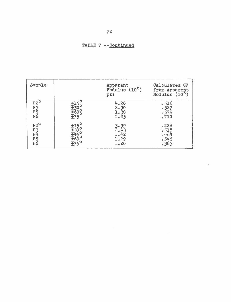
TABLE 7 --Continued

Sample Apparent , Modulus (10°) psi

Calculated ©from Apparent Modulus (106)

P2b +15° 4.20 .516P3 +30° 2.30 .327P5 ±60q 1.30 «579P6 ±75 1.25 .710P2C +15° 3»39 .228II S°5

2.431.42 .518.464P5 +60° 1.29 .545P6 ±75° 1.20 .383

7 2

73

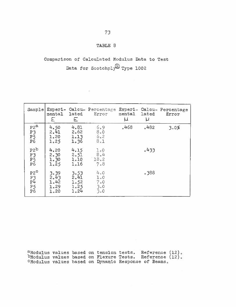
TABLE 8

Comparison of Calculated Modulus Data to TestData for Scotchpl3@ Typ< 1002

Sample Experi­mental£

Calcu­latedE

PercentageError Experi- Calcu- Percentage mental lated Error

U UP2a 4.50 4.81 6.9 .468 .482 3.0#P3 2.41 2.62 8.0P 5 1.20 1.13 6.2P6 1.25 1.36 8,1P2b 4.20 4.15 1.0 .433P3 2.30 2.51 8.4P5 1.30 1.10 18.2p6 1.25 1.16 7.8P2° 3-39 3.53 4.0 0 U) 00 00P3 2.43 2.41 1.0P4 1.42 1.52 7.0P5 1.29 1.25 3o0P6 1.20 1.24 3.0

aModulus values based ^Modulus values based cModulus values based

ononon

tensionFlexureDynamic

tests. Reference (12). Tests. Reference (12;. Response of Beams.

7^

error incurred by calculating multiple and oblique angle properties from single layer properties* It is obvious that the error is slight and calculation of multiple layer properties is justified* The three sets of data are now complete. A summary of the data to be used in the calculation of the dynamic properties of the cantilevered plates is shown in Table 9«

Flexural Vibration Response of Cantilevered Laminated Orthotropic Plates

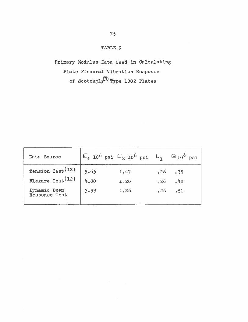
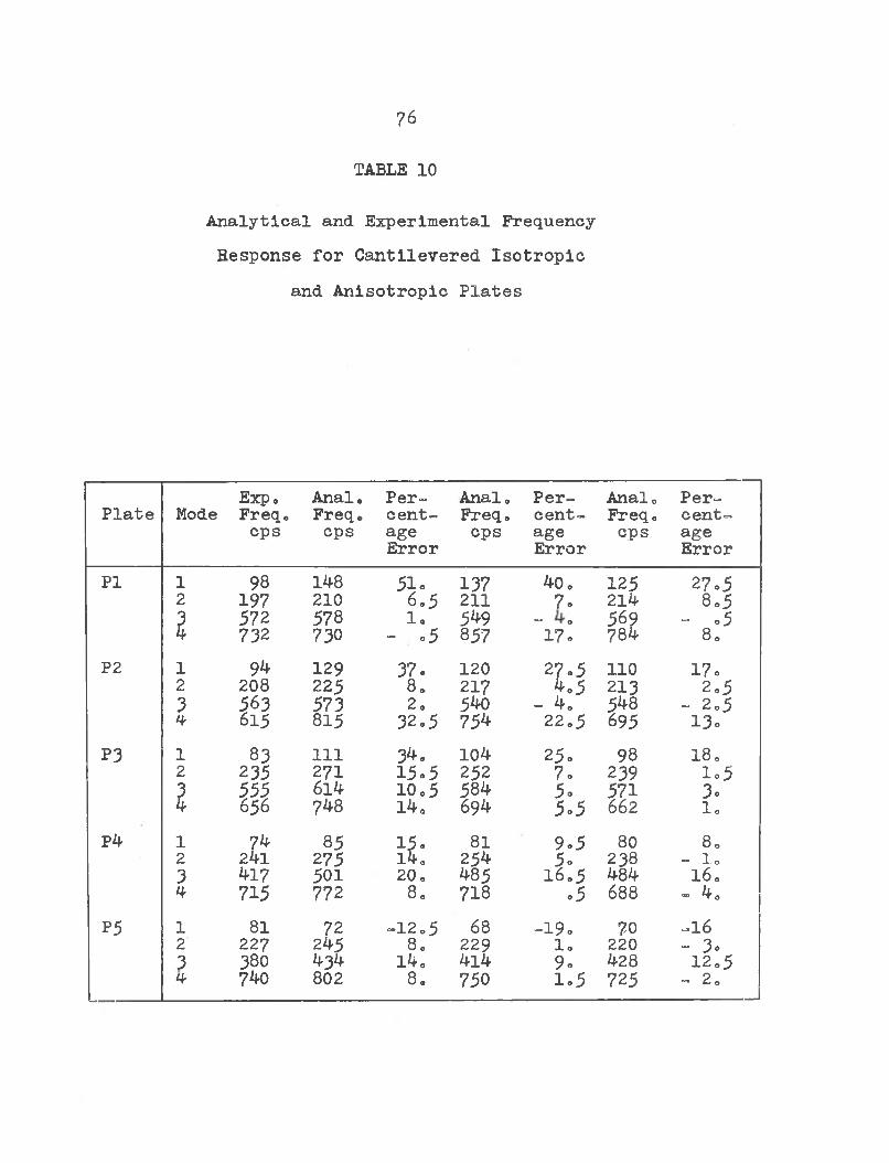
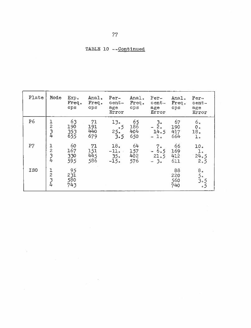
The flexural vibration response of cantilevereds laminated orthotropic plates was determined using equation 71. The three sets of modulus data (Table 9) were used for each of the plates (Table 5) PI through P7* The response of each plate was calculated on an I*B*M* 70*K) digital computer using the program in Appendix A. The analytical frequencies were checked against the experi- mental and a summary of this data is shown in Table 10*The experimental frequencies were obtained by driving the plates with a loudspeaker driver* The driver was connected to the plate by a post with two sided tape on the end toward the plate and the other end rigidly attached to the driver* The post was attached as close as possible to the clamped edge of the plate to minimize the change in boundary conditions which result from

75

TABLE 9

Primary Modulus Data Used in Calculating Plate Flexural Vibration Response

of Scotchplj^ Type 1002 Plates

Data Source ET-L 106 psi E72 io6 psi U ! S i o 6 psi

Tension Test -*- ) 5-65 1.4? .26 -35Flexure Test^^) 4.80 1.20 .26 .42Dynamic Beam Response Test 3-99 1.26 .26 -51

76

TABLE 10

A n a ly t ic a l and E xperim ental Frequency

R esponse fo r C a n tile v e r e d I s o t r o p ic

and A n iso tr o p ic P la t e s

Plate Exp. Mode Freq. cpsAnal.Freq.cps

Per­cent­ageError

Anal.Freq.cps

Per­cent­ageError

Anal.Freq.cps

Per­cent­ageError

PI 1 98 148 51« 137 40. 125 27.52 197 210 6.5 211 7. 214 8.53 57 2 57 8 1. 549 “» 0 569 - .54 732 730 “ .5 857 17. 784 8.P2 i 94 129 37. 120 27.5 110 17 02 208 225 8. 217 ^0 5 213 2.53 563 573 2. 540 - 4. 548 - 2.54 615 815 32.5 754 22.5 695 l3oP3 1 83 111 34. 104 25. 98 18.2 235 271 15.5 252 7. 239 io53 555 6l4 10.5 584 5. 571 3.4 656 748 14. 694 5.5 662 1.P4 1 74 85 15. 81 9.5 80 8.2 241 275 14. 254 5. 238 - 1.

3 41? 501 20. 485 16.5 484 16.4 715 772 8. 718 .5 688 - 4.P5 1 81 72 -12.5 68 -19. 70 -162 227 245 8. 229 1. 220 - 3.

3 380 434 14. 4l4 9. 428 12.54 740 802 8. 750 1.5 725 - 2.

77

TABLE 10 --Continued.

Plate Mode Exp.Freq.cps

AnaloFreq.cpsPer­cent­ageError

Anal.Preq.cps

Per­cent­ageError

Anal.Preq.cps

Per­cent­ageErrorP6 1 63 71 13. 65 3. 67 6.2 190 191 .5 186 - 2. 190 0.

3 353 440 25. 40 4 14.5 417 18.h 655 679 3-5 650 - 1. 664 lo

p7 l 60 71 18. 64 7. 66 10.2 167 151 -11. 157 - 6.5 169 1.3 330 445 35 0 402 21o5 412 24.54 595 586 -15. 576 - 3o 611 2»5

ISO l 95 88 8.2 231 220 5°3 580 560 3o54 7^3 740 °5

78

loading the plate with a point load. The plates could be excited with the post attached as close as one quarter of an inch from the clamped edge of the plate. To determine the natural frequencies a strain gage was attached to each plate and the strain output was displayed on an oscilloscope as each plate was excited. At a natural frequency a large change in strain amplitude could be discerned. The frequency at each peak amplitude was then recorded.

The mean percentage errors of analytical versus experimental frequencies are shown belows

Run 1, modulus data from tension tests (12)s mean error 15.0$.

Run 2S modulus data from flexure tests (12), mean error 10,3$.

Run 3> modulus data from dynamic beam tests9 mean error 8,1$.

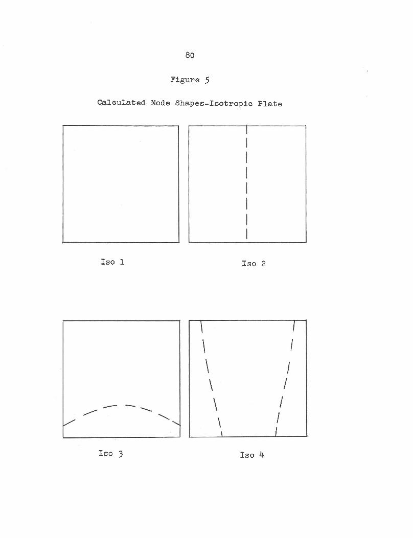
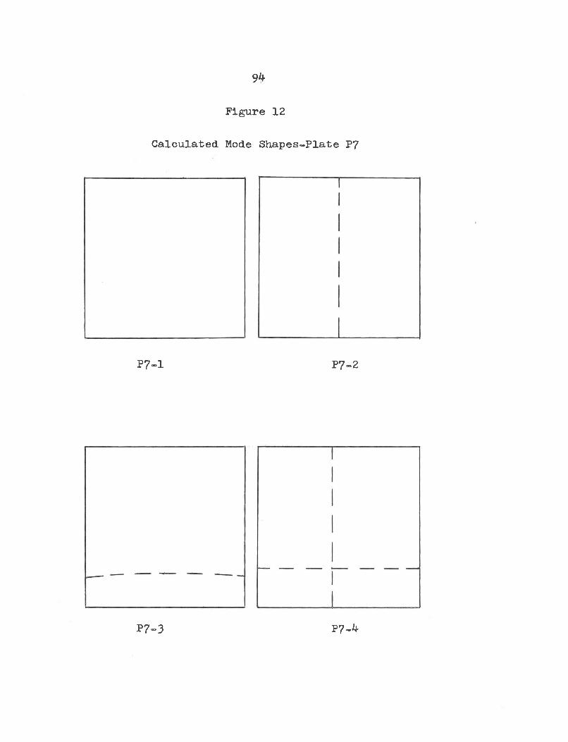
The plate response data shows the best correl­ation with the modulus data taken from the dynamic beam tests. Based on this conclusion the analytical mode shapes were drawn for each of the plates and compared with the experimental mode shapes. The figures 6 through 12 show the analytical mode shapes and the Plates III through IX show the experimental mode shapes.

If E. = E 2 , M.g , © = 0 ° and G ~ -- — ----1 2 ' 2 LI + M3

79

the orthotropic plate equations reduce to isotropic plate equationso Figure 5 and Plate II show the analytical and experimental mode shapes for an Isotropic plate„ Again, this data was acquired through the IoB0M0 7040 computer utilizing the program in Appendix A„

80

Figure 5

Calculated Mode Shapes-Isotropic Plate

Iso 1 Iso 2

Iso 3 Iso

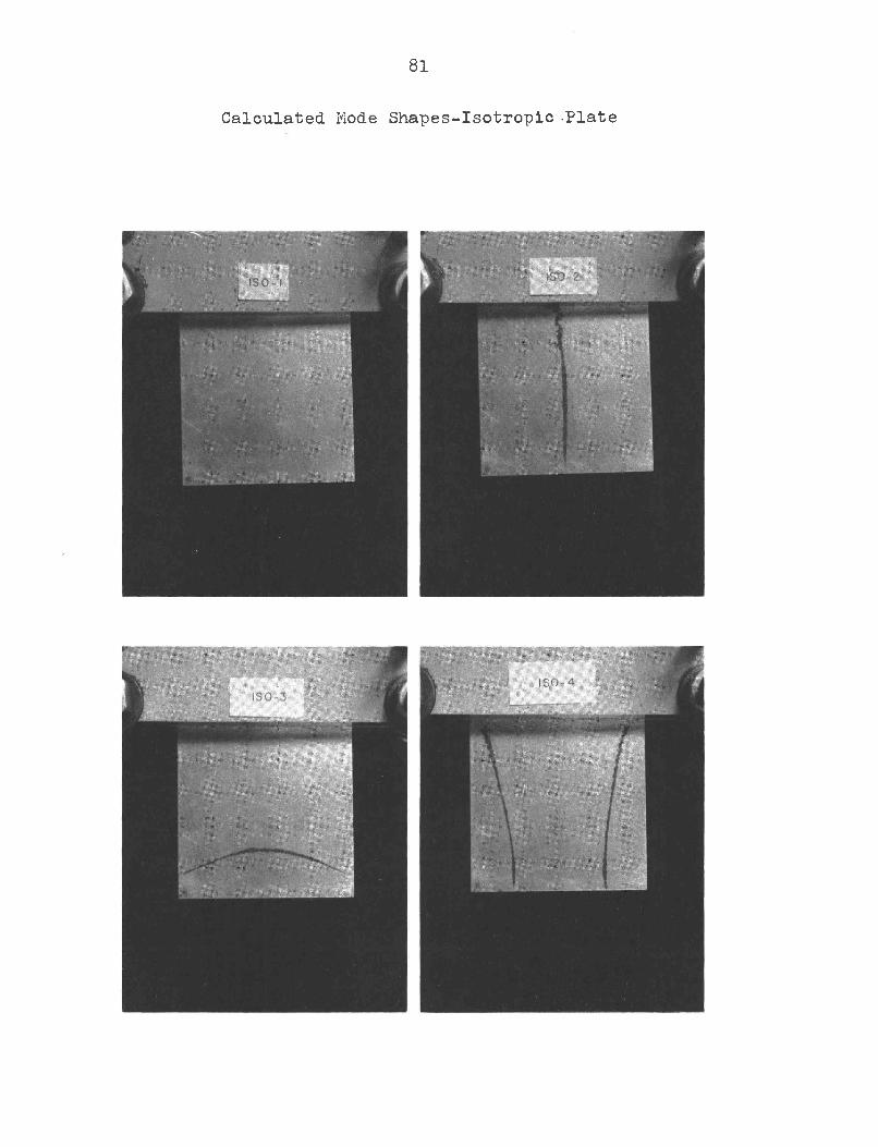
81

Calculated Mode Shapes-Isotropic -Plate

82

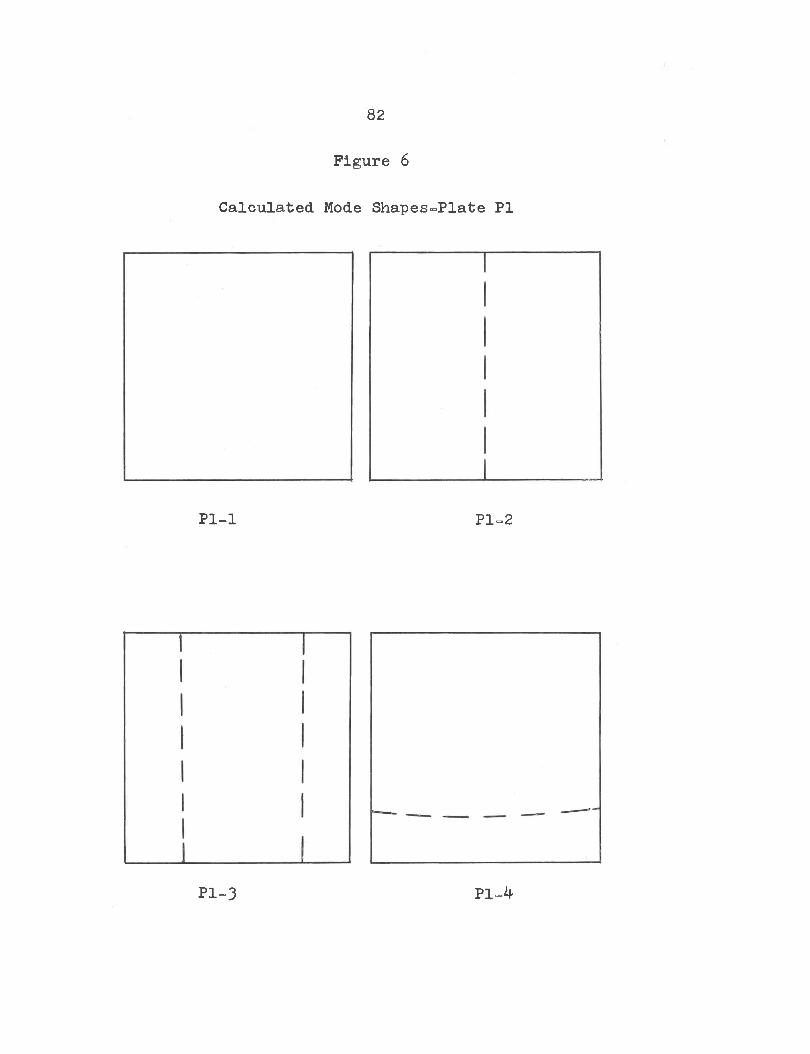
Figure 6

Calculated Mode Shapes-Plate PI

Pl-1

Pl-3 Pl-4

Pl~2

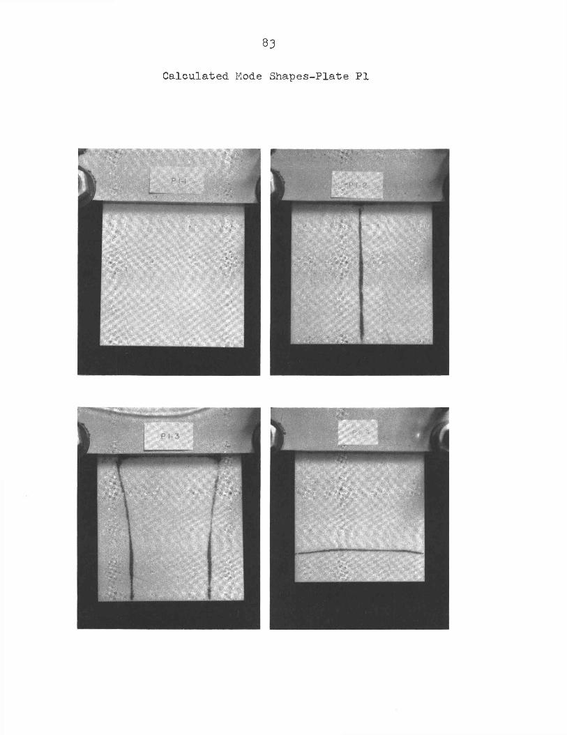
83

Calculated Mode Shapes-Plate PI

84

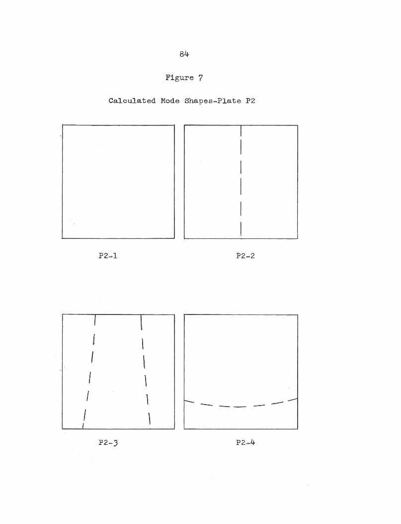
Figure 7

Calculated Mode Shapes-Plate P2

P2-1 P2-2

P2-4’P2-3

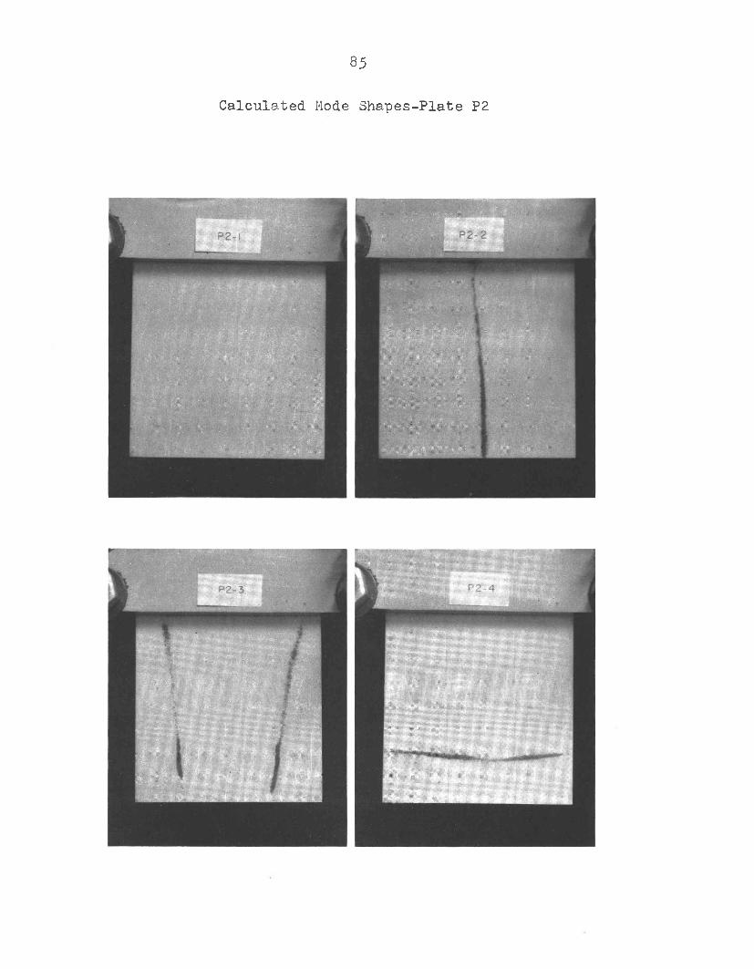
85

Calculated Mode Shapes-Plate P2

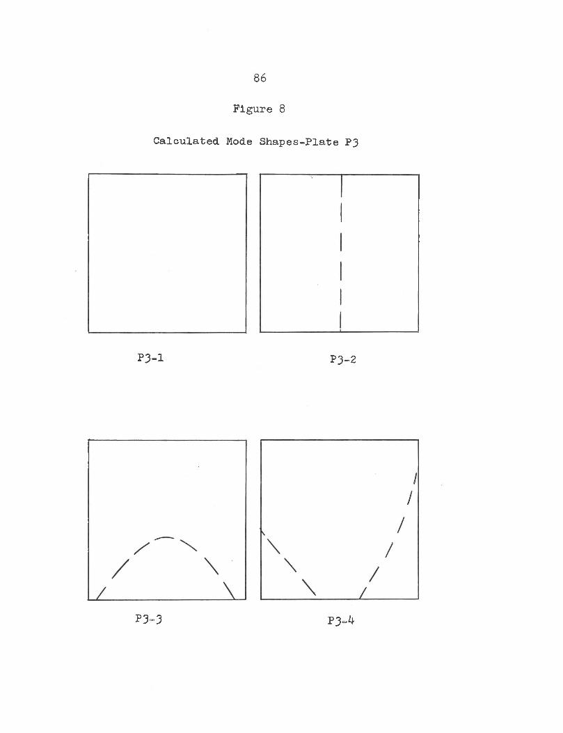
86

Figure 8

Calculated Mode Shapes-Plate P3

P3-3

P3-2P3-1

P3“^

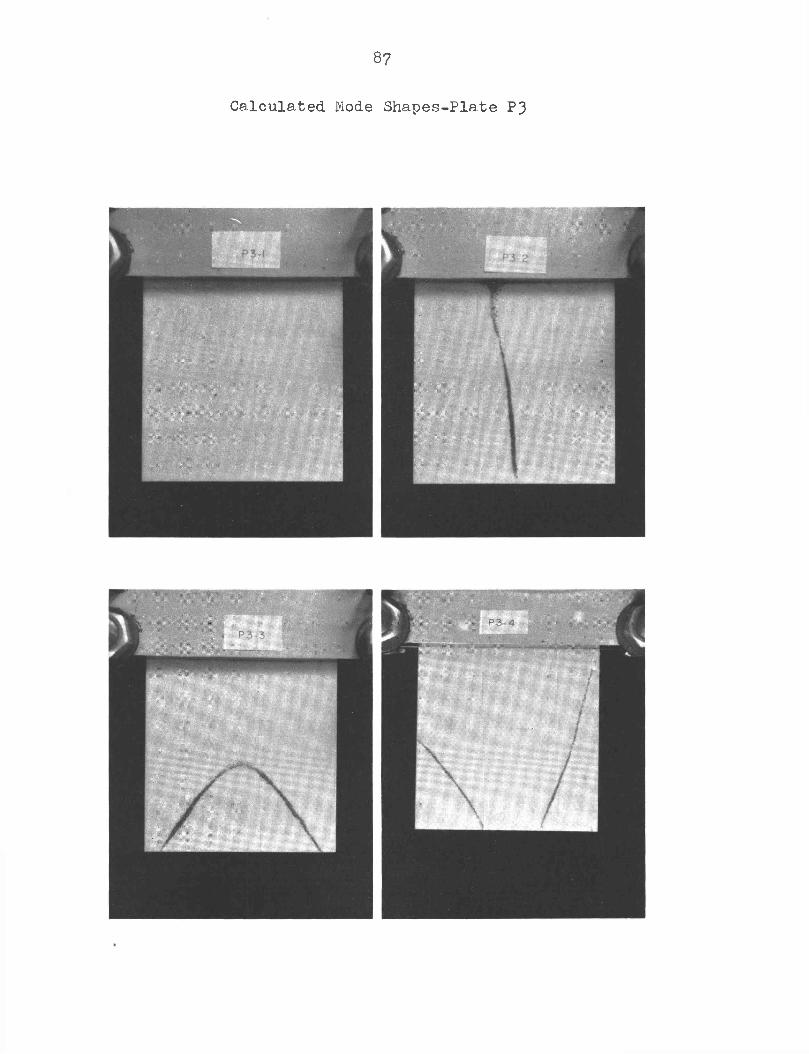
Calculated Mode

87

Shapes-Plate P3

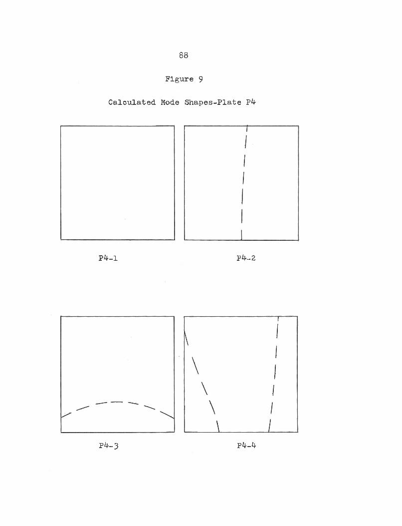
88

Figure 9

Calculated Mode Shapes-Plate P4

P4-1

P^-3 P^-4

P4-2

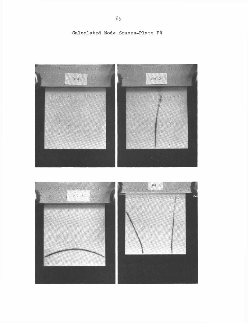
Calculated Mode

89Shapes-Plate P4

90

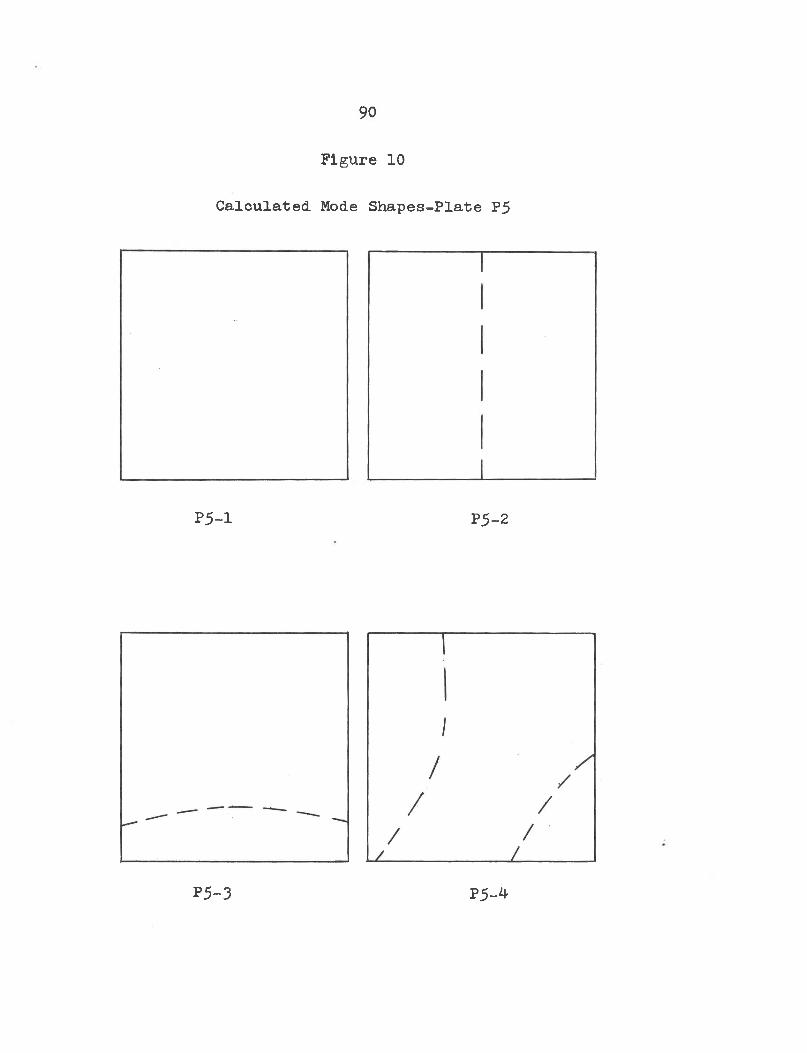
Figure 10

Calculated. Mode Shapes-Plate P5

P5-1

P5-3 P5-4

P5-2

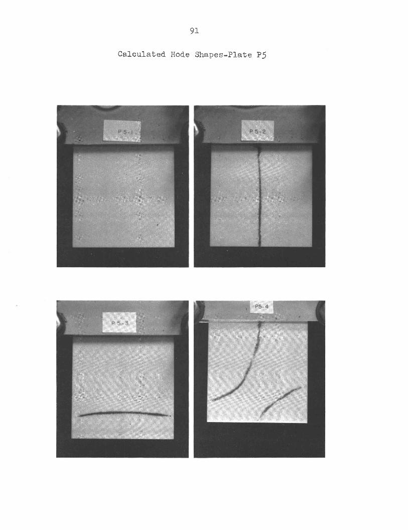
Calculated Mode

91Shapes-Plate P5

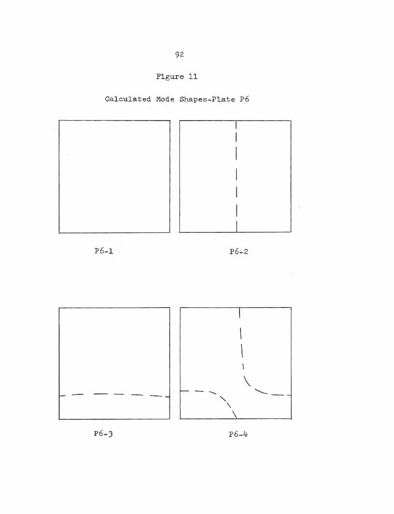
92

Figure 11

Calculated Mode Shapes-Plate P6

P6-1 P6-2

P6-4P6-3

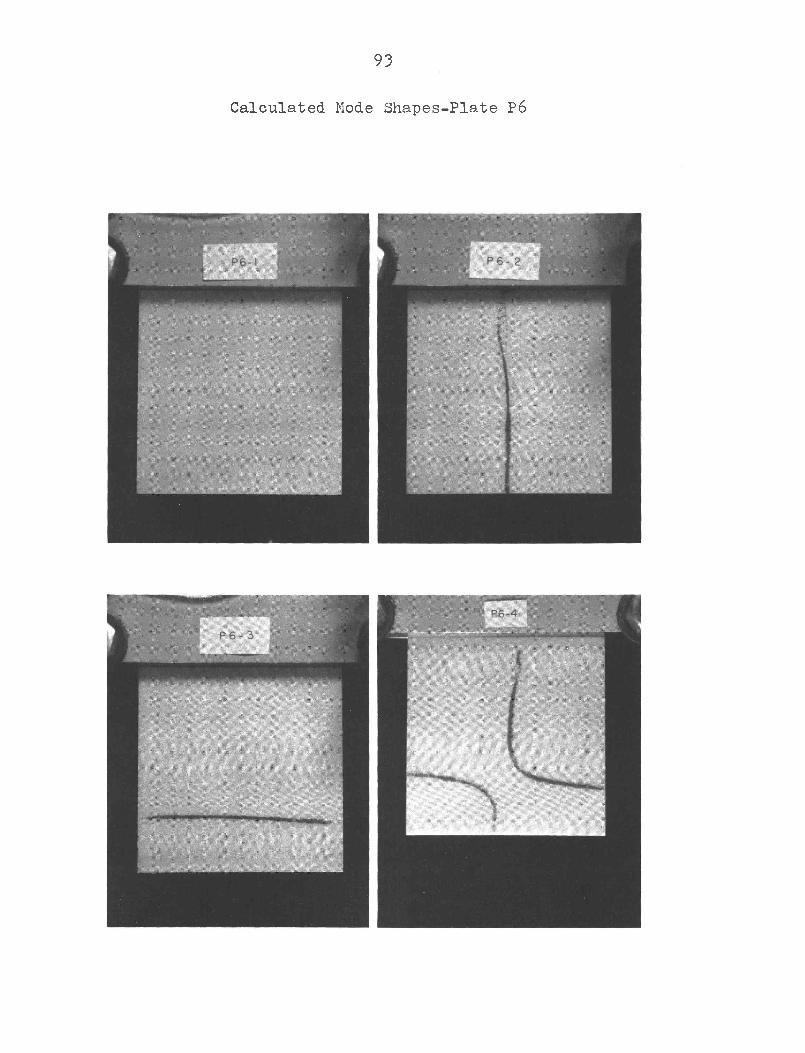
93

Calculated Mode Shapes-Plate P6

9^

Figure 12

Calculated. Mode Shapes-Plate P7

P7-1

P7-3 P7-4

P7-2

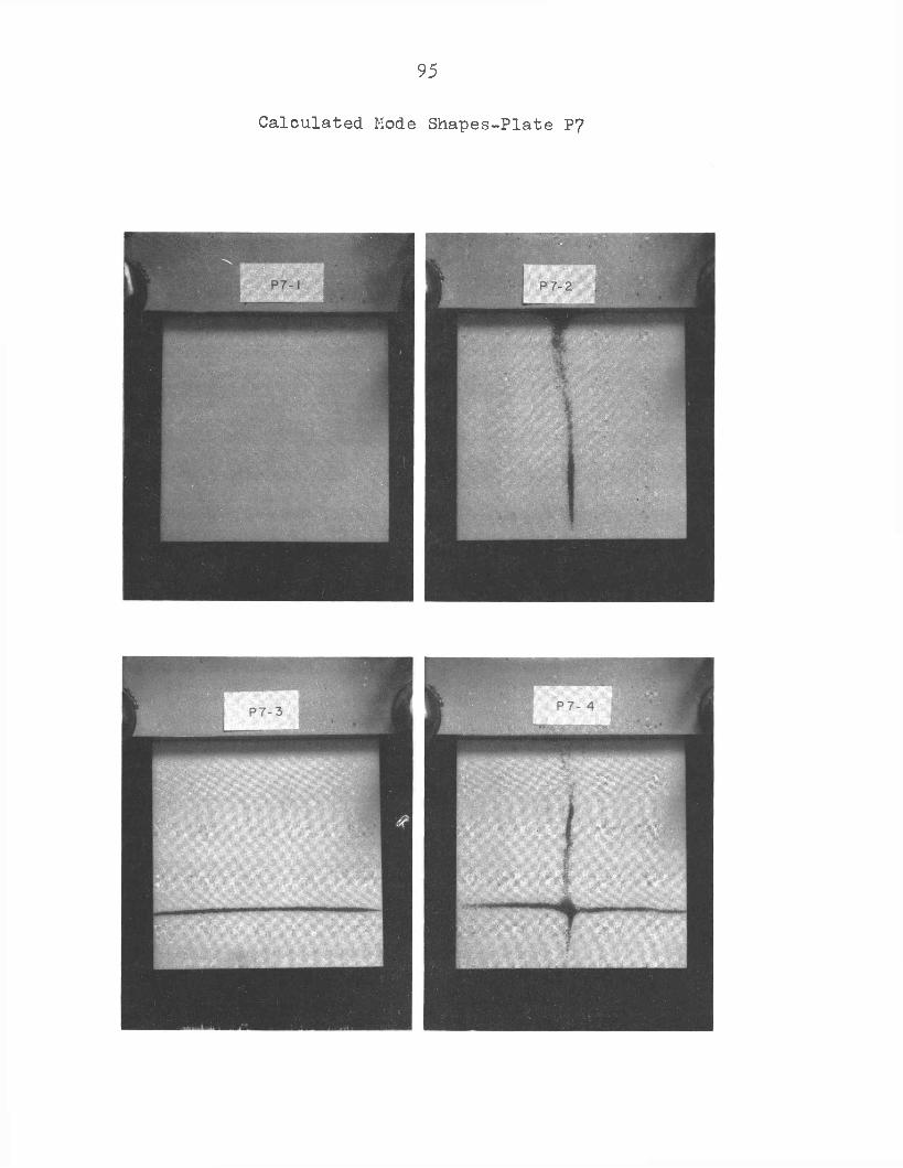
Calculated Mode

95S h a p e s-P la te P7

CHAPTER IV

SUMMARY, CONCLUSIONS AND

RECOMMENDATIONS

The e q u a tio n s have been d ev e lo p ed to c a lc u la t e th e

f le x u r a l v ib r a t io n resp o n se o f a lam in ated o r th o tr o p ic

p la t e fo r th e c a se where th e lam inae a r e p la c e d p a ir w ise

about th e m idd le su r fa c e o f th e la m in a te , The s p e c i f i c

c a se o f a c a n t i le v e r e d , lam in ated o r th o tr o p ic p la t e w ith

th e above m entioned lam inae r e s t r i c t i o n s on th e lam inae

o r ie n t a t io n has been so lved ,, The s o lu t io n has been

programmed fo r an I,B .M , 704-0 computor in F ortran IV

language,. The e l a s t i c p r o p e r t ie s fo r S co tch p ly® ty p e 1002

p a r a l l e l f ib e r g la s s r e in fo r c e c p l a s t i c have been o b ta in ed

and th e S co tch p ly® ty p e 1002 p la t e s were used to v e r i f y

th e a n a ly t i c a l developm ent e x p e r im e n ta lly „

The a n a ly t i c a l and exp erim en ta l r e s u l t s checked

so c lo s e l y i t may be conclu ded th a t a s a t i s f a c t o r y

m athem atical model has been o b ta in e d .

T h is a n a ly s is cou ld probab ly be extend ed to any

o r th o tr o p ic la m in a te i f th e fundam ental e l a s t i c p r o p e r t ie s

£T, s E a , M, and G a re known.

T h is study has produced th e computer program and

97

g e n e r a l a n a ly s is p r o ced u res . W hile th e r e s u l t s seem to

be e x c e l le n t th e r e are some problem s which sh ou ld be

co n sid er ed in th e fu tu r e .

An in v e s t ig a t io n o f th e con vergence o f th e R itz

method sh ou ld be con d u cted . The work o f K antorovich and

K rylov (10) dem onstrated th a t i f an i n f i n i t e number o f

term s a re co n sid er ed in th e s o lu t io n s e r i e s (e q u a tio n 48)

th e s o lu t io n w i l l ten d toward an e x a c t s o lu t io n . T his•* isu g g e s ts th a t an in c r e a se d number o f term s shou ld le a d to

a s t a b le d e c r e a s in g v a lu e o f each n a tu r a l freq u en cy . T his

d e c re a se i s ex p ected b ecau se th e in a c c u r a c ie s le a d to a

s o lu t io n which i s an upper bound fo r th e e x a c t s o lu t io n .

E quation 71 co u ld be programmed fo r any number o f term s

from p = / , q = / t o p - 5 s q - 7 which would

a llo w fo r th e s o lu t io n to c o n s id e r from one to 35 term s

in th e s o lu t io n s e r i e s (e q u a tio n 7 1 ) , A pilot o f number

o f term s v e r su s n a tu r a l freq u en cy a t each n a tu r a l freq u en cy

sh ou ld in d ic a te w hether or n o t th e s e r i e s i s ten d in g toward

co n v erg en ce .

F u rther exp erim en ta l v e r i f i c a t i o n o f th e a n a ly s is

tech n iq u e co u ld be o b ta in ed by t e s t in g p la t e s o f d i f f e r e n t

la y e r geom etry and a s p e c t r a t i o .

APPENDIX

APPENDIX A

COMPUTER PROGRAM FOR THE CALCULATION OF THE

FLEXURAL VIBRATION RESPONSE OF LAMINATED

ORTHOTROPIC PLATES

T his computer program was w r it t e n to compute th e

f l e x u r a l v ib r a t io n resp o n se o f c a n t i le v e r e d , lam in ated

o r th o tr o p ic p l a t e s . The program was w r it te n in F ortran IV

(12) and programmed fo r u se In an I.B .M . 70^0 d i g i t a l

com puter.

The in p u t card s are a s f o l lo w s ;

Card 1 (Format (1H+, ^E15«8)) in p u ts a r e ;

E ( , th e modulus o f e l a s t i c i t y o f th e b a s ic

com p osite m easure in th e s t i f f e s t d ir e c t io n ? E2 , th e

modulus o f e l a s t i c i t y o f th e com p osite m easured perpen­

d ic u la r t c E (.;A4/ P o is so n s r a t io measure by th e s t r a in

in th e 2 d ir e c t io n d iv id e d by th e s t r a in In th e 1

d ir e c t io n ; G , th e com p osite sh ear m odulus.

Card 2 (Format (1H+, 5E15®8) in p u ts a r e ;

Laminate th ic k n e s s ( in c h e s ) , p la t e le n g th

( in c h e s ) , p la t e w id th ( in c h e s ) , p la t e mass

d e n s ity per cu b ic in ch and th e a n g le o f th e

p r in c ip le a x i s o f th e f i r s t la y e r to th e major

100

a x es o f th e p la t e (d e g r e e s )*

Card 3 (Format (1 2 , I I ) In p u ts a r e :

N, th e s i z e o f th e E igen v a lu e m atrix to be

co n sid er ed and NI, 0 i f no o f f l i n e outp ut i s

d e s ir e d and 1 i f o f f l i n e outp ut i s d esired *

The program i s d es ig n ed to compute th e v ib r a t io n

resp o n se fo r a p la t e which i s composed o f 12 la y e r s o f

equal th ic k n e s s o r th o tr o p ic la m in a e . The la y e r s must be

sy m m etr ica lly o r ie n te d about th e m iddle su r fa c e o f th e

p la t e and th e a n g le s must be o r ie n te d a s shown in Table

5.G iven th e proper in p u t in fo rm a tio n th e program

computes an 18 by 18 E igen v a lu e m atr ix o f th e ty p e g iv e n

in eq u a tio n 51» The r e a l E igen v a lu e s and E igen v e c to r

fo r each E igen v a lu e a re determ ined* An 18 term

d e f l e c t io n s e r i e s i s c o n str u c te d ; th e p la t e i s d iv id e d

in to 625 c o o rd in a te p o in ts and th e d e f l e c t io n a t each

p o in t i s computed.

The program o u tp u ts are th e f i r s t f i v e E igen

v a lu e s fo r th e p la t e , th e co rresp o n d in g E igen v e c to r fo r

each E igen v a lu e , th e freq u en cy in cps corresp on d in g to

each E igen v a lu e and th e mode shape a t each o f th e f i v e

fundam ental f r e q u e n c ie s . A l i s t i n g o f th e program i s

g iv e n on th e n e x t 17 p a g e s .

101

B ecause th e ty p e sp a c in g w i l l n o t a llo w a f u l l

72 c h a r a c te r w id th , some o f th e F ortran s ta te m en ts have

been broken,. I f a program i s keypunched from t h i s t e x t

punch th e l i n e s a s shown* Where c o n t in u a tio n card s are

needed th e n e c e ssa r y c h a r a c te r i s typed*

102

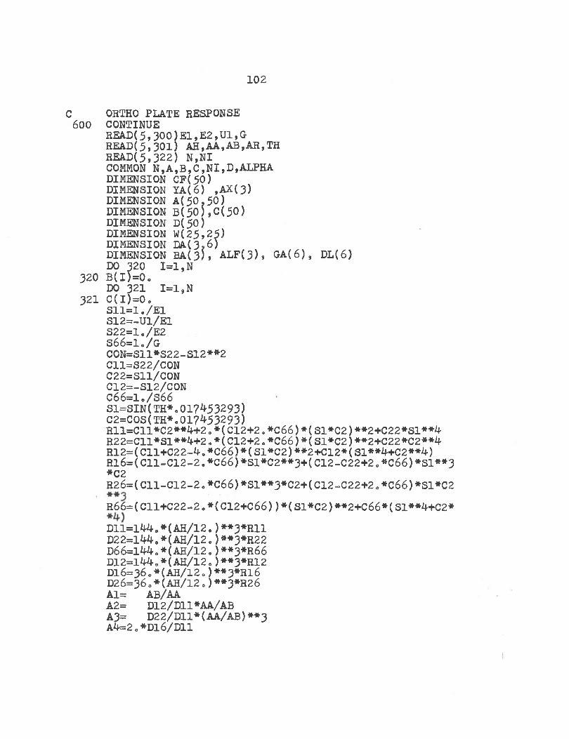
C ORTHO PLATE RESPONSE600 CONTINUE

READ(5,300)E1,E2,U1,G READ(5» 301) AH,AA,AB,ARSTH READ(5»322) N,NI COMMON N,A,B,C,NI,D,ALPHA DIMENSION CF(50)DIMENSION YA(6 ) ,AX(3)DIMENSION A (5 0 ,5 0 )DIMENSION B (5 0 ),C (5 0 )DIMENSION D(50)DIMENSION W (25,25)DIMENSION DA(3 ?6 )DIMENSION B A (3), ALF(3)» GA(6 ) , DL(6 )DO 320 1 = 1 ,N

320 B( I )=0 .DO 321 1 = 1 ,N

321 C (I)= 0 .S l l= lo /E l S12=-U1/E1 S 2 2 = l./E 2 S66= l . /GC0N=S11*S22-S12**2 C11=S22/CON C22=S11/CON C12=-S12/CON C66= l . / S 66S1=SIN(TH*o017453293)C2=C0S(TH*o017^53293)R ll=C ll*C 2**^ + 2» * (C12+2. *C6 6 ) * ( S1*C2) **2+C22*Sl**4 R 22= C ll*S l**4+ 2„ * (C12+20 *C6 6 ) * ( S1*C2) **2+C22*C2**4 R12=(C11+C22^»*C66)*(S1*C2)**2+C12*(S1**4+C2**^) R l6= ( C 11-C 12-2. *C6 6 )*Sl*C 2**3+(C 12-C 22+2. *C6 6 )*S1**3 *C2R26=(C11-C12-2 . *C6 6 )*Sl**3*C 2+(C 12-C 22+20 *C6 6 )*S1*C2

R66= ( C11+C22-2. * ( C12+C66)) * ( S1*C2) **2+C66*(S1***H-C2*

D ll= l4 4 0 * (AH/12. ) **3*R11 D22=l*j4. *( AH/12. ) **3*R22 D66=l*j4„*(AH/12„ )**3*r66 D 12= l44 .* (A H /l2 .)**3*R 12 D16=36 o * (AH/12 » )* * 3*R16 D26=36. * (AH/12. ) **3*R26 Al= AB/AA A2= D12/D11*AA/ABA3= D22/D11*(AA/AB)**3A^=2 „ *D16/'D11

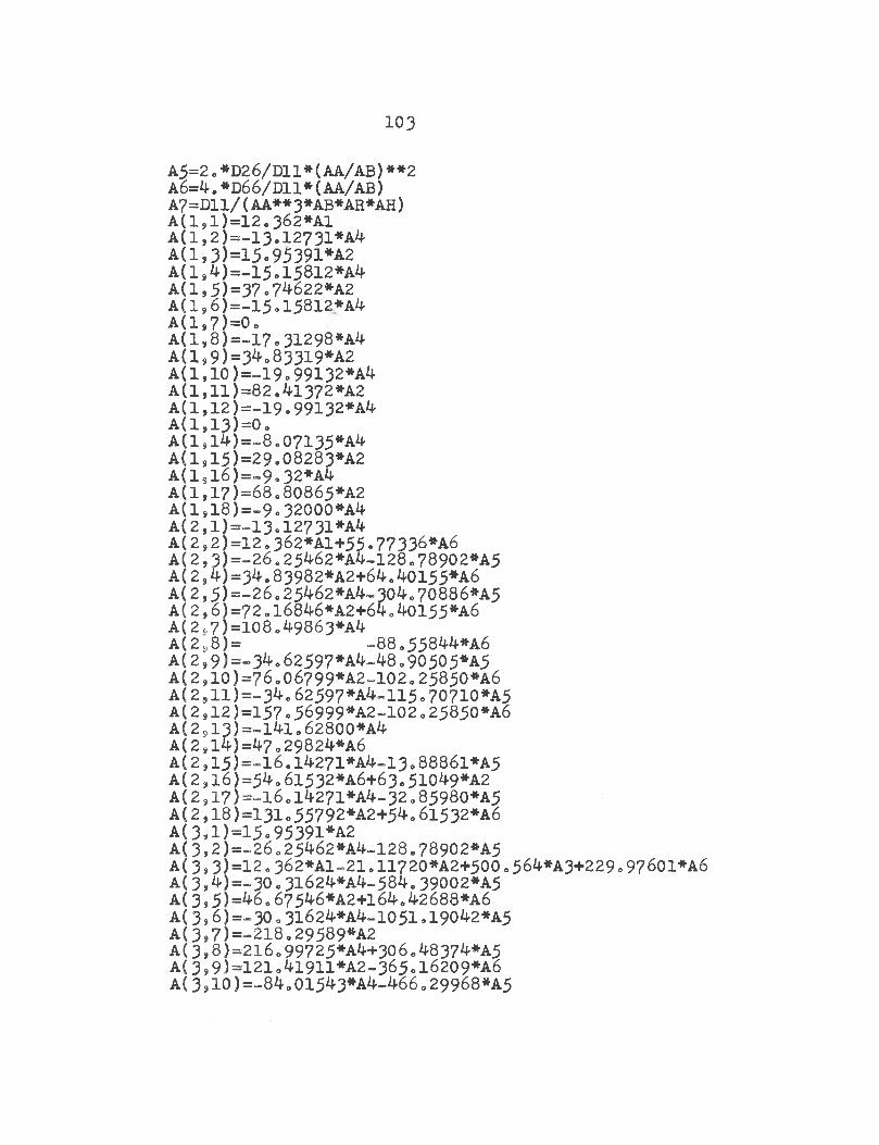
103

A5=2. *D26/D11*(AA/AB)**2 A6=4. *D66/D11*(AA/AB)A7=D11/(AA**3*AB*AR*AH)A (1 s1)=12.362*A 1A (1 ,2 )= -13 .12731*A ^a (i ,3)=15.95391*A2A (1 ,4 )= -1 5 .1 5 8 1 2 * A 4A (1 s5)=37.7^622*A 2A (1 96 )= -1 5 015812*A^A(1s7)=0oA (1 , 8 )= —17„31298*A4A (1 s9)= 3^ o83319*A2A (1 ,1 0 )= -1 9 o99132*A4A ( l ,l l )= 8 2 .4 l3 7 2 * A 2A (1 ,12 )= -19 .99132*A ^a (i ,13)=o .a(i9i4)=-8.07135*a4A (1 S15)=29.08283*A 2A ( l 9l6 )= -9 .3 2 * A 4A (l,17)= 68»80865*A 2A(1 91 8 )= -9 o32000*A4A (2 91 )= » 1 3 012731*A4a ( 2 92)=12o362*A 1+55.77336*a6A (2 93 )= -26 .25^ 62*A 4-128o78902*A5A (2 9 4)=34.83982*A 2+64,40155*A 6A (2 ,5 )= -2 6 o25^62*A4~30^.70886*A5A (2 , 6 )= 7 2 ol6846*A2+64„40155*A6A(2„7)=108„49863*A4A (2 s8)= -88 .55844*A 6A (2 99)=-3^o62597*A ^ -48o90505*A5A (2 910)= 76o06799*A 2-102o25850*a6A (2 9l l ) = - 3 4 e62597*A 4-ll5o70710*A 5A (2 s12)=157.56999*A2-.102»25850*A6A (2 s1 3 ) = - l 4 l o62800*A4A (2sl4)=47o29824*A 6A(2915)=““l6.1^-271*A4-13o8886l*A5A (2 si6)=5^o6l532*A 6+63o510^9*A2A (2 917)= -l6ol^271*A ^-32o85980*A 5A (2 ,1 8 )= 131 . 55792*A2+5406 i532*a6A (3 sl)= l5 „ 9 5 3 9 i* A 2A (3 92 )= ~ 2 6 o25^62*A4~128»78902*A5A (3 s3 )= 1 2 o362*A 1-21o11720*A2+500o56^*A3+229o97601*A6a ( 3 9^)=-30o3l62^*A ^-584„39002*A 5A( 3 ,5 ) =46 . 67546*A2+l64.42688*A6A (3 , 6 )=»30 o 3 l6 2 4 * A 4 -1 0 5 l. 19042*A5A (3,7)= -218»29589*A 2A(3,8)=216.99725*A^+30 6.48374*A5A {399)= 121»4 l911*A 2-365 .l6209*A 6A (3 s10)= »84„01543*A 4-466o29968*A5

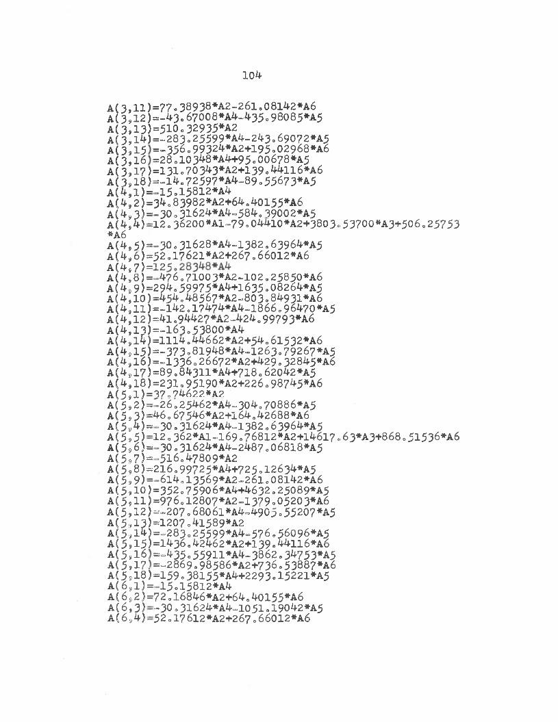
10^

A(3,H)A(3s12)A(3,13)A(3»l4)A(3»15A(3,l6A(3»17)A(3sl8)A(4,l)=A{4,2)=A(4S3)=A(4,4)=*A6A(4»5)=A(4*6)=A(4S7)=A(4S8)=A(499)=A(4,10)A(4,ll)A(4,12)A(4,13)A(49l4)A(4,15)A(4,l6)A(4,17)A{4918)A(5»l)- a ( 5 92 )= a(5,3)= A(594)= A(5s5) a ( 5 96 )= a (5.7)= a ( 5 , 8 )= A(5»9)= A(5,10) A(5911) A(5 j12) A(5A(5, .A(5.15) a (58i6

:i2!

A(5.17.A(5918)a (6,1)=A(692)= A(6,3)A(694)

=77.38938*A2-26l„08l42*A6=-43.67008*A4^35<,98085*A5= 510o32935*A2=-283o25599*A 4-243.69072*A 5 =-356„9932^*A2+195o02968*a6 =28 010 3^8*A*h-95 o 00 678*A5 =1 3 1 o 70 3^3 *A2 +1 39 o 4 4 l1 6 *a 6 =«l4„72597*A4»89o35673*A5

15<.15812*a4 3 4 o83982*A2+64o40155*a6

3 0 .3 l624*A 4-5840 39002*A5 12.36200*A1-79o04410*A2+3803<

30 . 31628*A4-1382.63964*A5 52»17621*A2+267o66012*A6io e476„71003*A2-102 .25850*A6

294o59975*A4+i635„08264*A5 = 454o48567*A 2-803o84931*a6 =-142 o17474*A4-1866.96470*A5 =4lo9442?*A2-424099793*A6 =-163o53800*A4 =1114044662*A2+54o6l532*A6 =-373o81948*A 4^1263.79267*A 5 =-1336 o26672*A2+429.32845*A6 =89.84311*A4+718 o 62042*A5 =231„95190*A2+226o98745*a6 37„74622*A2

2 6 o25462*A 4-304o70886*A5 46„67546*A2+164042688*A6 30. 31624*a4-1382 . 63964*A5

12„362*Al-l69.?68l2*A2+l46l7< 30 o 3l624*A4~2487.068l8*A5 516o47809*A2

216o99725*a4+725012634*A5 6l4„13569*A2-26l„08l42*A6 =352 o 7590 6*A4+4632„25089*A5

=976o12807*A 2-13?9o05203*a6 =-207 o 68Q6i*A4~4905 <> 55207*A5 =1207o4l589*A2 =-283 o 25599*a4 -576„56096*A5 =1436„42462*A2+139 o 44ll6*A6 =“435 o 5 5 9 H * a 4 -3 8 6 2 . 34753*A5 =-2869o98586*A2+736o53887*A6 =159o38155*A4+2293o15221*A5

15o15812*a4 72„l6846*A2+640 4oi55*A6 ■-30«3l624*A4-1051.19042*A5 52 o17 6l2*A2+267 „ 6 6 0 1 2 *a 6

53700*A3+506„25753

63*A3+868o51536*a 6

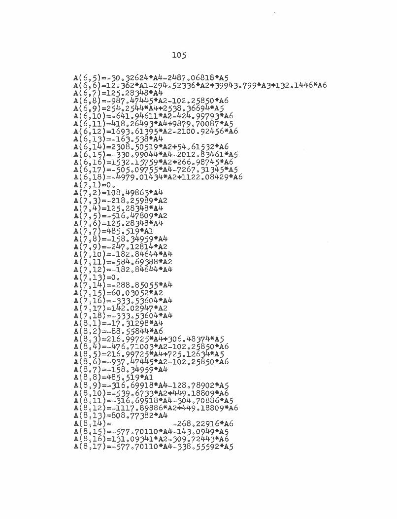
A(695)=-300 32624*A4-2487„06818*A5A(6,6)=12.362*A1-29^.52336*A2+399^3.799*A3+132.1^6*A6a (6,7)=125o28348*a4A(6,8)=-987 « 47445*A2~102 o 25850*A6a( 6,9) =254. 2544*A4+2538 . 36694*A 5A(6,10)=-64l„946ll*A2-424.99793*a 6A(6,11)=4l8.26493*A4+9879.70087*A5A(6912)=l693o6l395*A2-2100o92456*A6A(6S13)=-163.538*A4A{6,l4)=2308o505l9*A2+54o6l532*A6A(6s15)=-330o99044*A4-2012.8346i*A5A(6sl6)=l532„l5759*A2+266„98?45*A6A (6 917)=»505»09755*a4-.7267„31345*A5A(6918)=-4979o01434*A2+1122o08429*A6A (7 91 ) = 0 oA(7,2)=108o49863*A4 A(7>3)=-218„25989*A2 A(794)=125.28348*A4 A(7s5)=-516o47809*A2 A(796)=125.28348*a4 A(7 9 7)=485 o 519*A1 A( 7 9 8)=-158 . 34959*A4 A(7 9 9)=-247 o128l4*A2 A( 7 910)=-182.84644*A4 A(79H ) = “584069388*A2 A(7,12)=-182 o 84644*A4 A(7»13)=OoA(79l4)=-288o85055*A4A(7,15)=60o03052*A2A(7si6)=-333°53604*a4A(7917)=1^2o02947*A2A{7918)=-333o53604*A4A(8S1)=-17o31298*A4A(8,2)=-88 o 55844*A6A(893)=216,99725*A4+306o48374*A5A(894)=-476„71003*A2-102,,25850*a 6A(8s5)=216099725*A4+725„12634*A5A(8,6)=-937.47445*A2-102.25850*A6A{8 s7)=-158.34959*A4A{8 s8)=4850 519*A1A(899)=-3l6o69918*A4-128„78902*A5A(8,10)=-539.6733*A2+449.18809*A6A(8,ll)=-3l6.69918*A4-304.70886*A5A(8 912)=-1117 o 89886*A2+449.18809*A6A(8913)=808„77382*A4A{8sl4)= -268.229l6*A6A(8915)=-577„70110*a4-143o0949*A5A(8s16)=131o09341*A2-309«»72443*A6A(8,17)=-577»70110*a4-338„55592*A5

105

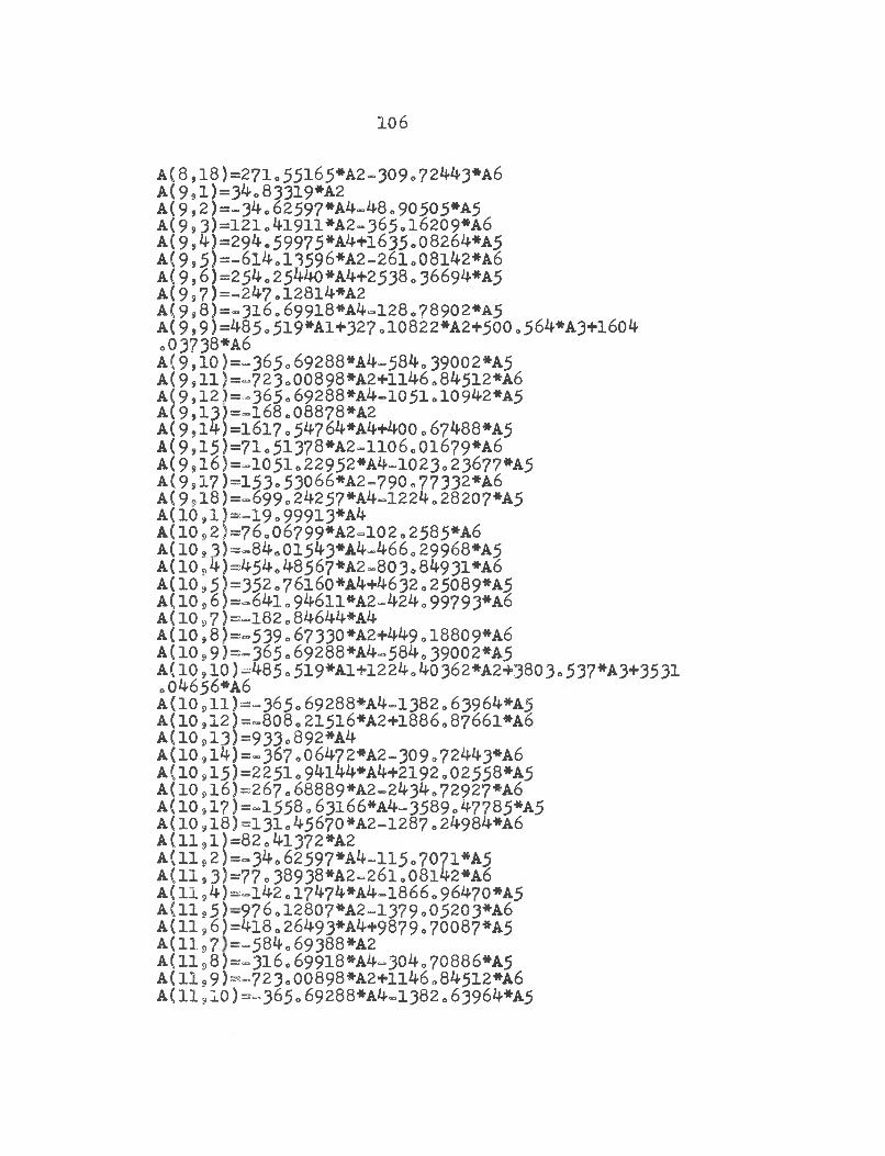
A(8,l8)=27lo55l65*A2-309o72^3*A6 A(9.1)=3^o83319*A2 A(9,2)=-34„62597*A4-48„90505*A5 A(9s 3)=121o4l911*A2-365ol6209*A6 A(994)=294.59975*A4+i635„08264*A5A(9»5)=-6l^o13596*A2-26lo08l^2*A6A( 9 * 6) =254* 25440*A4+2 538.36694*A5A(9S7) =-24-7 . 128l4*A2A(998)=-3l6o699l8*A4-128„78902*A5a (9»9)=485.519*Al+327.l0822*A2+500 o564*A3+1604o03?38*a6A(9,10)=-365<»69288*A4-584o39002*A5A(9911)=“723o00898*A2+1146o84512*A6A(9»12)=-365.69288*A4-1051.10942*A5A(9,13)=”168o08878*A2A(9,14)=1617 .54764*A4+400.67488*A5A(9»15)=71<.51378*A2-ll06o0l679*A6A(99l6)=-l05lo22952*A4-l023o23677*A5A(99l7)=l53o53066*A2-790o77332*A6A (9 s,1 8 )= -6 9 9 o24257*A4-1224o28207*A5A (1 0 s1 ) = - 1 9 o99913*A4A(10<,2)=76o06799*A2-102o2585*a6a(1093)=-84o01543*a4-466o29968*A5A(10e,4)=454o48567*A2-803<.84931*A6A(l095)=352o76l60*A4+4632o25089*A5A(10,6)=-64lo 946ll*A2-4240 99793*A6A(10 9 7)=“182o 84644*A4A(10s8)=-539o67330*A2+449„18809*A6A(10,9)=-365.69288*A4-5840 39002*A5A(10 910)=485 o 519*A1+1224„40362*A2+3803» 537*A3+3531„04656*a 6A(10s,ll)=-365o69288*A4-l382o63964*A5A(10,12)=-808.215l6*A2+l886.8766l*A6A(10s,13)=933o892*a 4A(l09l4)=-367o06472*A2-309o72443*A6A(10915)=2251o9i+l^*A4+2192o02558*A5A(109l6)=267o68889*A2-2434„72927*A6A(10917)=-1558o63l66*A4-3589o47785*A5A(10,18)=131.45670*A2-1287 o24984*A6A(1191)=82o41372*A2A{ll92)=-34o62597*A4-ll5,7071*A5A(ll,3)=77o38938*A2-26lo08l42*A6A (1 1 s4 ) = - 1 4 2 o17474*A4-1866„96470*A5A(lls5)-976ol2807#A2-l379„05203*A6A(1196)=418o26493*a4+9879o70087*A5A(lls7 =-584o69388*A2A (1 1 98 ) = - 3 1 6 o69918*A4-304o70886*A5A(1199)=“72 3o 00898*A2+ll46„84512*A6A(119IO)==365.69288*A4-13820 63964*A5

106

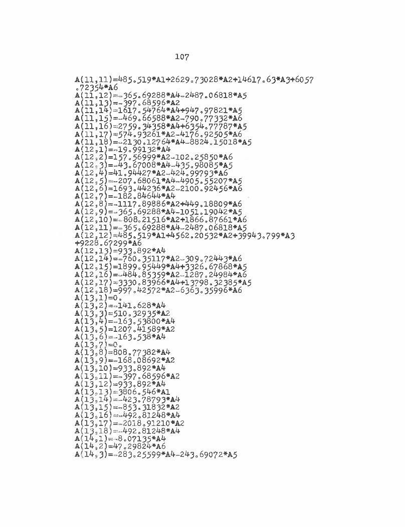
A(11, 11)=485o 519*Al+2629 o 73028*A2+l46l7. 63*A3+6057 „72354*a6A(11s12)=^365o69288*A4»2^87o06818*A5A(11s13)=-397o68596*A2A (ll, i£)=1617o 5^764*a4+947 o 97821*A5A(11s15)=“^69o66588*A2-790o77332*a 6A(ll,l6)=2759.3^358*A4+6354o77787*A5A(11,17)-57^093261#A2-4i76„92505*a6A(11s18)=-2130o12764*A4-.8824„15018*A5A(1291)=-19o99132*A4A(12,2)=157 o 56999*A2-102o25850*A6A(12,3)=-43o67QQ8*A4~435o98085*A5A(12s4)=41o94427*A2-»424o99793#a 6A(1295)““207o68061*A4=4905o55207*A5A(12s6)=1693o44236*A2^2100o92456*A6A (12,7)=-182o84644*A4A(1298)=-1117o89886*A2+449818809*A6A(1299)=-365o69288*A4^1051o19042*A5A(X2910)= ~808 o21516*A2+1866o87661*A6A(12,ll =“365»69288*a4^2487o06818*A5A(12912)=485o519*A1+4562„20532*A2+399^3o799*A3+9228o67299*A6A(12913)=933„892*a4A(129i4)==760o35H7*A2^309o?2443*a6A(12s15)=1899o95^9*A4+3326o67868*A5A (12,16 )=->484o85359*A2-1287 0 24984*a6A(12 917)=3330 o 83966*A4+13?98.32385*A5A(12 s18)=997 o42572*A2=6363o 35996*A6A(13,l)=0oA(13»2)==l4lo 628*A4A(1393)=510o32935*A2A(1394)==i63„53800*a4A(1395)=1207o41589*A2A(l396)==l63o538*A4A (1 ^ 71—0A(1398)=808o77382*A4A(13s9)-‘=168o08692*A2A(l35l0)=933o892*A4A{13911)=«397o68596*A2A(l38l2)=933o892*A4A(13913)=3806o5^6*A1A(l39l4)=-423078793*A4A(13s15)==853»31832#A2A(13 ,16 )=-492o 81248*A4A (13 s> 17) =“2018 o 91210 *A2A{13918)=^492o81248*A4A(l49l)=-8o07135*A4A(l492)=47„29824*A6A{149 3) =-283»25599*a4=243o 69072^5

107

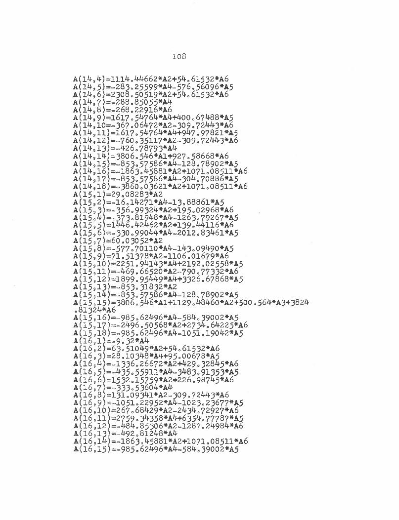
108

A ( l4 s4 )= X ll4 044662*A2+5406l532*A6A (l^ » 5 )= -2 8 3 o25599*A4»576o56096*A5a ( 14 , 6)=2308„50519*A2+5^c 6 i532*a6A ( l4 s7)=-288<,85055*A4A (1458)=-268o229X6*A6A (1 4 ,9 )= 1 6 1 7 ,5 4 7 64*A4+400„67488*A5A (14 ,10= ~ 367 o06472*A2~309o72443*A6A ( l4 9ll)= l6 l7„54764*A 4+ 947o97821*A 5A ll4 ,l2 )= -7 6 0 o 3 5 1 1 ?* A 2 -3 0 9 o 7 2 4 4 3 #A6A ( l4 s l3)==.426o78793*A4 'A (l4 ,l4 )= 3806o546*A l+ 927o58668*A 6A ( l4 sl5 j= »853o57586*A 4-l28 .?8902*A 5A (l4 ,l6 )s -1 8 6 3 .4 5 8 8 l* A 2 + l0 7 1 o 0 8 5 ll* A 6A ( l4 9l7 )= -8 5 3 o 5 7 5 8 6 * A 4 -3 0 4 o70886*A5A ( l4 sl8)=»3860o03621*A 2+1071o08511#A6A (1 5 ?l ) = 2 9 o08283*A2A (1 5 ,2 )= -l6 .1 4 2 7 1 * A 4 -1 3 o 8886l*A5A (15 s3 )“ “ 358 o99324*A2+195o02968*a 6A ( l5 94 j= -3 7 3 c8 l9 4 8 * A 4 -l2 6 3 o 7 9 2 6 7 #A5A (1 5 ,5 )= 1446042462*A2+139„4 4 h 6 * a 6A (15 ,6 )= -330„99044*A 4-2012 .8346 l*A 5A (15 s7 )= 6 0 o03052*A2A (15,8)= -577o70110*A 4-l43o09490*A 5A (1599)^71o51378*A 2=1106o01679*A6A (15910)=2251o94143*A 4+2192o02558*A5A (1 5 ,ll)a -4 6 9 .6 6 5 2 0 * A 2 -7 9 0 .7 7 3 3 2 * A 6A (1 5 912)^1899o95449*a4+3326«67868*A 5A (1 5 913)=-853o31832*A 2A (15sl4)=«=853„57586*A4-128o78902*A5A (15915)=3806 0 546*AX+X129 • 4846g*A2+500„564*A3+3824„81324*A6A{1 5 ,16)=^985o 62496*a4-584„390Q2*A5 a ( 1 5 ,1 7 )= -2 4 9 6 o 50568*A2+2734o 64225*a6 A (1 5 ?1 8 )= -9 8 5 o62496*A4-1051o19042*A5 A ( i6 91 )= -9 „ 3 2 * a4 A ( l6 92)=63o5l049*A 2+54o6l532*A6 A (1 6 93)=28.10348*A4+95o00678*A5 A (x 6 945=-l336o266?2*A 2+429o32845*A 6 A (1 6 ,5 )s=435o 5 5 9 ll* A 4 -3 4 8 3 , 91353*A5A (1 6 96)= 1532015759*A2+226»98745*A6 A (i6 ,7 )= -3 3 3 „ 5 3 6 o 4 * a 4 A ( l6 s8 )= 1 3 lo0934l*A 2-309o72443*A 6 A ( l6 s9)=-l051o22952*A 4-l023o23677*A 5 A(1 6 ,1 0 )= 2 6 7 *68429*A2-2434o 72927*A6 A ( l6 9ll)= 2759o34358*A 4+ 6354077787*A5 A (1 6 ,1 2 )= -4 8 4 0 85306*A 2-1287„24984*A6 A(1 6 ,1 3 )= -4 9 2 o 81248*A4 A { l6 9l4 )= -l8 6 3 o 4 5 8 8 l* A 2 + 1 0 7 1 o08511*A6 A { l6 ,1 5 )=-985o 62496*A4-584„39002*A5

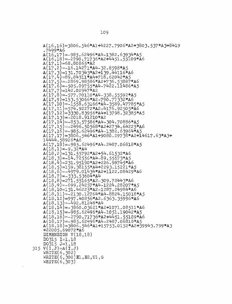
A ( l6 ?l6 )= 3806o5^ 6*A l+ 4227o7906*A2+3803o53?*A3+84l9o7^99*A6A ( l6 s1 7 )= “985<> 62496*a4-1382.6393^*A 5A ( l6 s 18) =-2790 o 717 36*A2+4451 «,55109*A6A (1 7 ,1 )= 6 8 o80865*A2A (1 7 s2 )= -1 6 014271*A 4-3208598*A5A (17,3)= 131o703^ 3*A 2+l39o^ l l6 * A 6A (1 7 s4 )= 8 9 o84311*A^+718o620^2*A5A( 17 9 5 )= ““2869 .9 8 5 8 6 ^ 2 + 7 3 6 »53887*a6a ( 1 7 ,6 )= -505 o 0 9 7 5 5 ^ - 7 ^ 2 2 011^86*A5 A( 17 9 7 )=1^2 o 029^7*A2 A (17 ,8 )* -577 .70110*A 4-338 .55592*A 5a (1 7 j9)= 153°53066*A 2-790o7?332*a 6A ( l7 s10)= -1558 .63 l66*A 4-3589 .^ 7785*A 5A (1 7 ,ll)= 5 7 ^ .9 2 2 7 2 * A 2 -4 i7 6 .9 2 5 0 5 * A 6A (17»12 )= 3330 . 83956*a4+13798„32385*A5A (17913)=~2018o91210*A2A (1 7 ,1 4 )= » 8 5 3 .5 7 5 8 6 * A ^ 3 0 ^ o70886*A5A( 1 7 ,1 5 ) =-2^960 50568*A2+27 34 o 64225*A6A( 1 7 ,1 6 5 = -9 8 5 .62^96*A^-1382. 63964*A5A (1 7 .1 7 ) =380 6 . 546*Al+9080 0 297 38*A 2+l46l7 . 63*A3+1 ^ 4 058926*A6A (1 7 ,1 8 )= -9 8 5 .62^96*A 4-2487. 068l8*A5A (1 8 s1 ) = - 9 032*A4A ( l 8 ,2 ) = i 3 i 055792*A2+5406l532*A6A (1 8 9 3 )= - i4 072556#a4^89.55673*A 5A (1 8 s4 )= 2 3 1 o95190*A2+226„987+5*A6a {1 8 s5 )= 1 5 9 o38155*a4+2293<.15221*A5A(18 9 6)=-4979.01^3^*A 2+1122o08429*A6a ( 1 8 97 )= -3 3 3 0536o4*a4A (1898 = 271o55l65*A2»309o724^3*a6A (1 8 s9 )= “6 99 o24257*A 4-1224o28207*A5A (18 s1 0 = 1 3 1 .46225*A2=1287. 2^984*A6A (1 8 ,1 1 )= -2 1 3 0 o12764*A 4-8824(>15018*A5A (18 s1 2 )= 9 9 7 c40856*A 2-6363o35996*a 6A (1 8 s1 3 )= -^ 9 2 o81248*A^A ( l8 sl4 )= ^ 3 8 6 0 o03621*A2+1071o08511*A6A(18<,15)=“985°62496*A 4~1051o19042*A5A(18 916 )= -2 7 9 0 .7 1 7 36*A 2+445l0 55109*a6A ( l8 s17j=-985o62496*A 4-2^8?e068l8*A 5A (1 8 918 )= 3 8 0 6 o546*A1+15753.0152*A2+399^3.799*A3+ 22005=69072*A6DIMENSION V(1 8 ,1 8 )D0315 1=1s18 D0315 J=1»18V( Is J )=A( 1 9 J )WRITE(69302)WRITE(6 9 3 0 0 )El 9 E2 9 U1s G WRITE(69303)

109

315

110

3io

211

212

323

326

255

256

213

3^3334335336

WRITE(6,301)AH,AA,AB,AR,TH D0310 J=1,18WRITE(6,311)J,A(J,1),J,A(J,2),J,A(J,3),j,a(j,4 WRITE(6,3l6)J,A(J,5)»J>A(J96)?J,A(J,7),J>A(J,8/ WRITE(6,314)J,A(J,9),J,A( J,10),J,A(J,11),J,A(J,12) WRITE(6,4ll)J,A(J,13),j }A(J,14),J,A(J,15)»J,A(J,l6) WRITE(6,412)J,A(J,17),J,A(J,18)DO 211 K=1,N DO 211 L=l9N A(K,L)=A(K,L)/5000 o CALL EIGN(N,A,B,C,NI)DO 212 K=1,N C(K=C(K)*5000o CALL ORD(N,C,NI)DO 323 1=1,N

D(I)=Q«DO 324 1=1,5ALPHA=C(I)DO 326 J=1,N DO 326 K=1,N A( J ,K)=V( J ,K)CALL VCTR(A,D,N,ALPHA)DO 255 JJ=1.N CF(JJ)=D(JJ)BIG=ABS(CF(l))DO 256 JJ=2,N BIGA=ABS(CF(JJ))IF(BIGA0GToBIG) big=bigaCONTINUEWRITE(6,342) BIGDO 213 K=1,ND(K)=D(K)/BIGWRITE(6,342)C D(IA),IA=1,18)AOM=SQRT(A?*ALPHA)/(36Oo*o017453293)WRITE(6,215) AOM BOM=S QRT(ALPHA)WRITER 6,342) BOM WRITE(60214)ALPHA GO TO 343 CONTINUE DO 334 K=l,6 DA(1,K)=D(K)DO 335 K=7,12 DA(2,K-6)=D(K)DO 336 K=13,18 DA(3,K-12)=D(K)BA(l)=lo8?5104l BA(2)=4o6940911 BA(3)=7o854?574

Ill

ALP(l)=07340955 ALF(2)=1»0184644 ALF(3)=o99922450 GA (1)=0.GA (2)=0 oGA(3)=4o7300408GA(4)=7,8532046GA(5)=10.995607GA(6)=l40l37l66DL(l)=0oDL(2)=0 oDL(3) = o 98250222DL(4)=i „0007773DL(5)=o99996645dl(6)=i.0000015DO 327 LA=1, 25DO 327 LB=1,25X1=LA-1Y1=LB-1X=Xl*AA/240Y=Yl*AB/24„W(LA,LB)=0oDO 333 M=l,3 DO 333 L=1,6 IF(L0EQ01) YA(l)=l0IF(L0EQ»2) YA(2)=SQRT(3J*0L-2o*Y/AB)IF(L0GE0 3) YA(L) = (EXP(GA(L)*Y/AB)+EXP(-(GA(L)*Y/

AB)))/2.+C0S(GA(L)1*Y/AB)-DL(L)*((EXP(GA(L)*Y/AB) ■~EXP( ■= (GA(L) *Y/AB)) )/20+SIN(GA(L)*Y/2AB)) XA(M)=(EXP(BA(M)*X/AA)+EXP(-(BA(M)*X/AA)))/2„~ C0S(BA(M)*X/AA)-ALF(1M)*((EXP(BA(M)*X/AA),EXP(- (BA(M)*X/AA)))/20-SIN(BA(M)*X/AA)) WA=DA(M<,L)*XA(M)*YA(L)

333 W(LAsLB)=W(LA,LB)+WA 32? CONTINUEDO 337 LA=1? 25

337 WRITE(6S338)(W(LASLB),LB=1,9)DO 339 LA=19 25339 write(6,338)(w(la,lb),lb=ios17)DO 341 LA=1? 25 34l WRITE(69 338)(W(LA,LB),LB=18,25)324 CONTINUE

GO TO 600338 FORMAT(1H ,9El4.7)322 FORMAT(12,II)304 FORMAT(E15o8)302 FORMAT(1H ,6X,2HF1912X,2HE2 s14X,2HU1914X,1RG)300 FORMAT(1H 94E15„8)

112

303 FORMAT(1H ,2X,9HTHICKNESS,8X,6HLENGTH,9Xs5HWIDTH» llx s 7HDENSITY,3X,18HFIRSTLA„,IX,2HTH)301 FORMAT(1H ,5E15„8)

342 FORMAT(1H »E15o8)214 FORMAT(1H 96HALPHA=9E15„8)311 FORMAT(1H 92X92HA(, 12,5H, l)=9E15o8,2X92HA( 8I295H9

2) = 9E15o8.2X,2H1A(,I295Hs 3)=9E15o892X92HA(9I2s5H9 4)=,E15o8)316 FORMAT(1H ,2X 92HA(9I2 ,5 H s 5 )= t EL5.8,2X,2HA<9I 2 S5H9

6}= ,E 15o8?2Xs2H 1 A (9I2 ,5 H 9 7 ) = sE15o892X92HA(sI 2 95H9 8 )= sE15o8)

314 FORMAT(1H s2X92HA(9I 2 95Hs 9) = »E15<>892X92HA( 9I 2 95H910) = sE15o8?2Xs2H 1A (>I 2 95H91 1 )= sE1508 s2X92HA(sI 2 95H912) =»E15o8)

411 FORMAT( 1H ,2X ,2H A (sI2 ,5 H ,13 )= oE 15o8 92X92HA(s I 2 s5 H ,l4 ) = sE15o8?2X*2H 1 A ( ,I 2 95Hj1 5 )= sE15o8,2X 92HA(sI 2 95H216)= SE15<,8)

215 FORMAT(1H f10HFREQUENCY=9E15o8412 FORMAT( 1H S2XS2HA( 9I 2 95H917) = 9E15<>892X92HA( 9I 2 95H918)

=9E15o8)END

113

SUBROUTINE ORD(N,C,NI)DIMENSION C(50),A(50), B(50), D(50)M=0K=0KG=1NA=0DO 10 L=1,N IF(C(L)) 11,11,1211 M=M+1A(M)=C(L)12 K=K+1 B(K)=C(L)10 CONTINUE20 AL=B(KC)DO 13 I=KC,K IF(B(I)oLEcAL) AL=B(I)

13 CONTINUEDO 15 J=KC,K IF(AL-B(J)) 14,16,1^

1k CONTINUE GO TO 15

16 B(J)=B(KC)B(KC)=AL KC=KC+1 GO TO 25

15 CONTINUE 25 NA=NA+1IF(5-NA) 1?,18S1817 CONTINUE GO TO 2018 CONTINUEDO 19 1=1,519 WRITE(6S23) B(I),I DO 2k 1=19K

2k C(I)=B(I)KK=K+1DO 21 I=KK ,N21 C(I)=A(I)23 FORMAT(1H S,E15<.8,4X,7HLAMBDA( ,11,1H))

RETURN END

114

SUBROUTINE EIGN (N,A,B DIMENSION A(50,50),B(50) CALL NTRI (A,B,N)CALL GRT (N,C,NI)RETURNEND

C,NI)c(50)

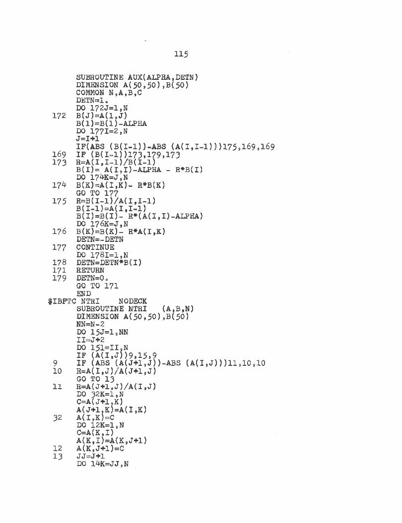
115

SUBROUTINE AUX(ALPHA,DETN)DIMENSION A(50,50),B(50)COMMON N,A,B,C DETN=1.DO 172J=1,N172 B(J)=A(l,J)B(1)=B(1)-ALPHA DO 1771=2,N J=I+1IP(ABS (B(I-1))-ABS (A(1,1-1)))175*1699169

169 IP (B(l-l))173>179>173173 R=A(I,I-1)/B(I-l)B(I)= A(I,I)-ALPHA - H*B(I)DO 17^K=J,N

17^ B(K)=A(I,K)- R*B(K)GO TO 177175 R=B(I-l)/A(I,1-1)B(I-1)=A(I,1-1)B(I)=B(I)- R*(A(I,I)-ALPHA)DO 176K=J,N176 B(K)=B(K)- R*A(I,K)DETN=-DETN

177 CONTINUEDO 1781=1,N178 DETN=DETN*B(I)171 RETURN179 DETN=0 o GO TO 171

END$IBFTC NTRI NODECKSUBROUTINE NTRI (A,B,N)DIMENSION A(50,50),B(50)NN=N-2DO 15J=1,NNII=J+2DO 151=11,NIF (A(I,J))9,15»99 IF (ABS (A(J+l,J))-ABS (A(I,J)))11,10,10

10 R=A(I,J)/A(J+l,J)GO TO 1311 R=A(J+l,J)/A(I,J)DO 32K=1,NC=A(J+l,K)A(J+l,K)=A(I,K)

32 A(I,K)=CDO 12K=1,N C=A(K,I)A(K,I)=A(K,J+l)12 A(K,J+l)=C13 JJ=J+1DO 1^K=JJ,N

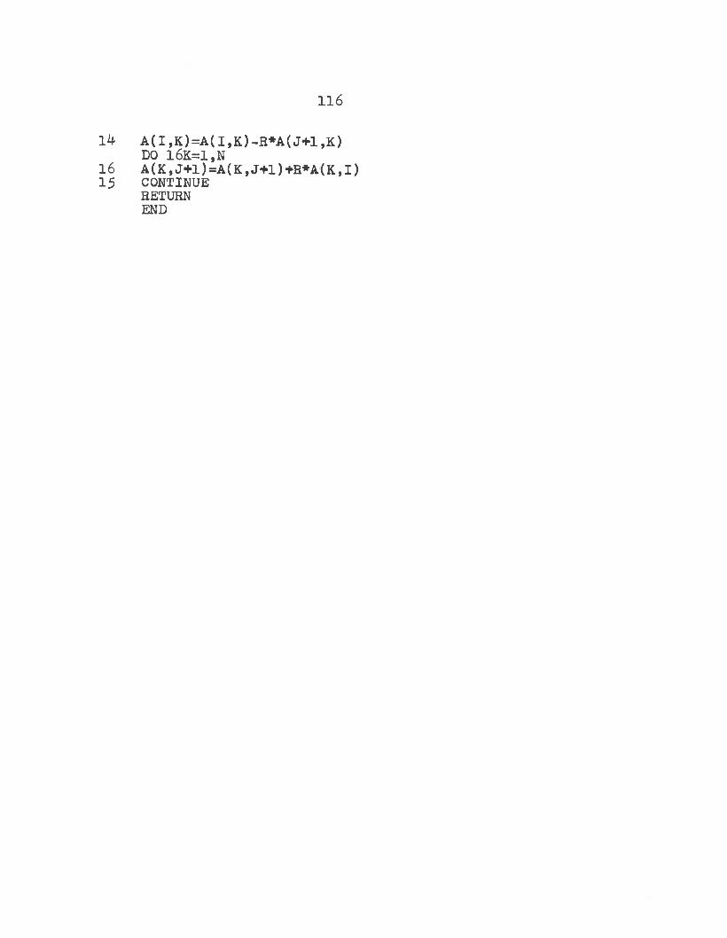
116

14 A(I,K)=A(I,K)-R*A(J+1,K)DO l6K=l,N16 A(K ,J+l)=A(K ,J+l)+R* A (K ,I)15 CONTINUE RETURN END

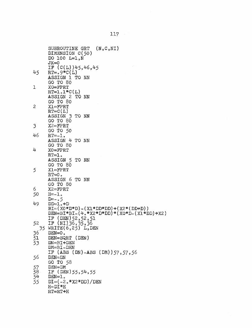
117

SUBROUTINE GRT (N,C,NI)DIMENSION C(50)DO 100 L=1,N JK=0IF (C(L))45,46,4545 RT=o9*C(L)

ASSIGN 1 TO NN GO TO 801 XO=FPRT RT=1„1*C(L)ASSIGN 2 TO NN GO TO 80

2 X1=FPRT RT=C(L)ASSIGN 3 TO NN GO TO 80

3 X2=FPRT GO TO 5046 RT=-1o

ASSIGN 4 TO NN GO TO 804 X0=FPRT RT=1

ASSIGN 5 TO NN GO TO 805 X1=FPRT

RT=0 •ASSIGN 6 TO NN GO TO 80

6 X2=FPRT50 H=-l„

D=-„549 DD=1.+DBI=(X0*D*D)-(X1*DD*DD)+(X2*(DD+D)) DEN=BI*BI-(4.*X2*D*DD)*(XO*D-(X1*DD)+X2)IF (DEN)52,52,5152 IF (NI)36,35,36 35 write(6925) l,den

36 DEN=0.51 DEN=SQRT (DEN)53 DN=BI+DEN DM=BI-DEN

IF (ABS (DN)-ABS (DM))57,57,5656 DEN=DN

GO TO 5857 DEN=DM58 IF (DEN)55954,5554 DEN=1055 DI=(-2.*X2*DD)/DEN H=DI*HRT=RT+H

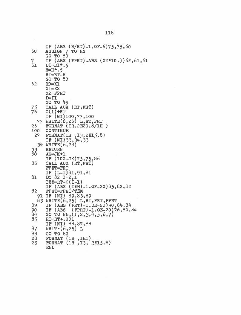
IF (ABS (H/RT)-1o0F-6)75,7596060 ASSIGN 7 TO NN GO TO 807 IF (ABS (FPRT)-ABS (X2*10.))62,61,6161 DI=DI**5 H=H*o5 RT=RT~H GO TO 8062 X0=X1 X1=X2 X2=FPRT D=DIGO TO 4975 CALL AUX (RT»FRT)76 C(L)+RT

IF (NI)100.77.100 77 WRITE(6,26) L,RT,FRT 26 FORMAT (I3,2E20o8/1H )100 CONTINUE 27 FORMAT(1H 9I3,2E15.8)IF (NI)33,34,33 34 WRITE(6,28)33 RETURN80 JK=JK+1IF (100-JK)75»75»8686 CALL AUX (RT,FRT)FPRT=FRTIF (L-l)8l,91,8l81 DO 82 1=2,L TEM=RT-C(I-1)IF (ABS (TEM)-1„OF-20)85,82,8282 FPRT=FPRT/TEM91 IF (NI) 89,83,89 83 WRITE(6s25) L,RT,FRT,FPRT89 IF (ABS (FRT) -1 <>0E-20) 90,84,8490 IF (ABS (FPRT)-1.0E-20)76,84,8484 GO TO NN,(1,2,3,4,5,6,7)85 RT=RT+,001IF (NI) 88.87,8887 WRITE(6,25) L88 GO TO 8028 FORMAT (1H ,1H1)25 FORMAT (1H ,13, 3E15.8)END

118

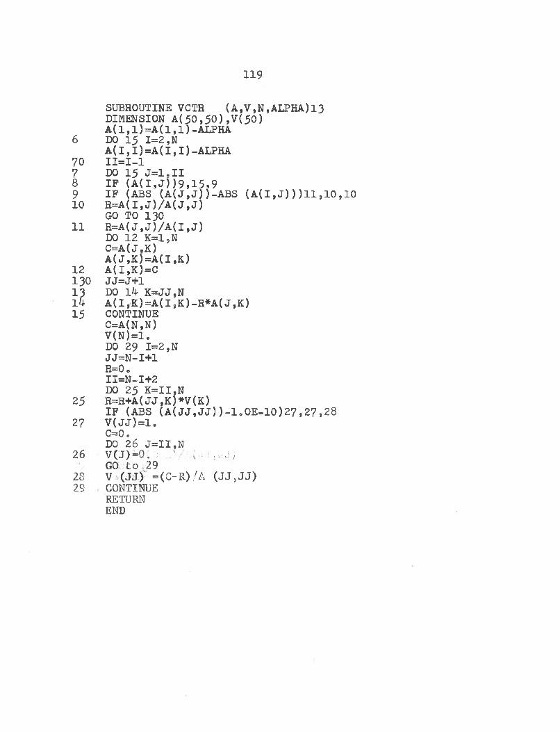
119

SUBROUTINE VCTR (A,V,N,ALPHA)l3 DIMENSION A(50,50),V(50)A(l,l)=A(1,1)-ALPHA6 DO 15 1=2,NA( I,I)=A(I,I)-ALPHA

70 11=1-17 DO 15 J=1.II8 IF (A(I#J))9,15,99 IF (ABS (A(J,J))-ABS (A(I,J)))ll,10,1010 R=A(I,J)/A(J,J)

GO TO 13011 R=A(J,J)/A(I,J)

DO 12 K=1,N C=A(J.K)A(J,K)=A(I,K)12 A(I,K)=C

130 JJ=J+113 DO 14 K=JJ,N1^ A(I,K)=A(I,K)-R*A(J,K)15 CONTINUE C=A(N,N)

V(N)=1„DO 29 1=2,N JJ=N-I+1 R=0 oII=N-I+2 DO 25 K=II,N25 R=R+A(JJ,K)*V(K)IF (ABS (A(JJ,JJ))-1»OE-IO)27 9 27 s 28

27 V(JJ)=1o C=0oDO 26 J=II,N26 V(J)=0.:; ■ ,uJ,

GO to 2928 V (JJ) = (G-R) / A (J J, J J)2S CONTINUE

RETUMEND

APPENDIX B

COMPUTES PROGRAM TO DETERMINE THE SHEAR MODULUS OF A SINGLE LAMINA FROM THE

APPARENT MODULUS OF A LAMINATE

This program is designed to compute G, the shear modulus of elasticity for a single laminae, from the apparent modulus of a laminate. The laminate must have its layers symmetrically placed about the middle surface of the laminate with each layer at alternating angles of plus and minus © from the major axes of the laminate. There must be an equal number of plus and minus layers.

The input card is as follows:Card 1 (Format (1H+, 7 E L 1 . 2 + ) ) inputs are:Ei , E a > M|, © and the apparent modulus

E, , E a and M| are the single layer properties determined by tension tests on unidirectional laminates tested with the load parallel and perpendicular to the principle axes. © is the ply angle and the apparent modulus is the measured modulus of elasticity of the laminate.

The program also calculates an apparent modulus assuming G in order to check the accuracy of the results. A listing of the program is given on the next page.

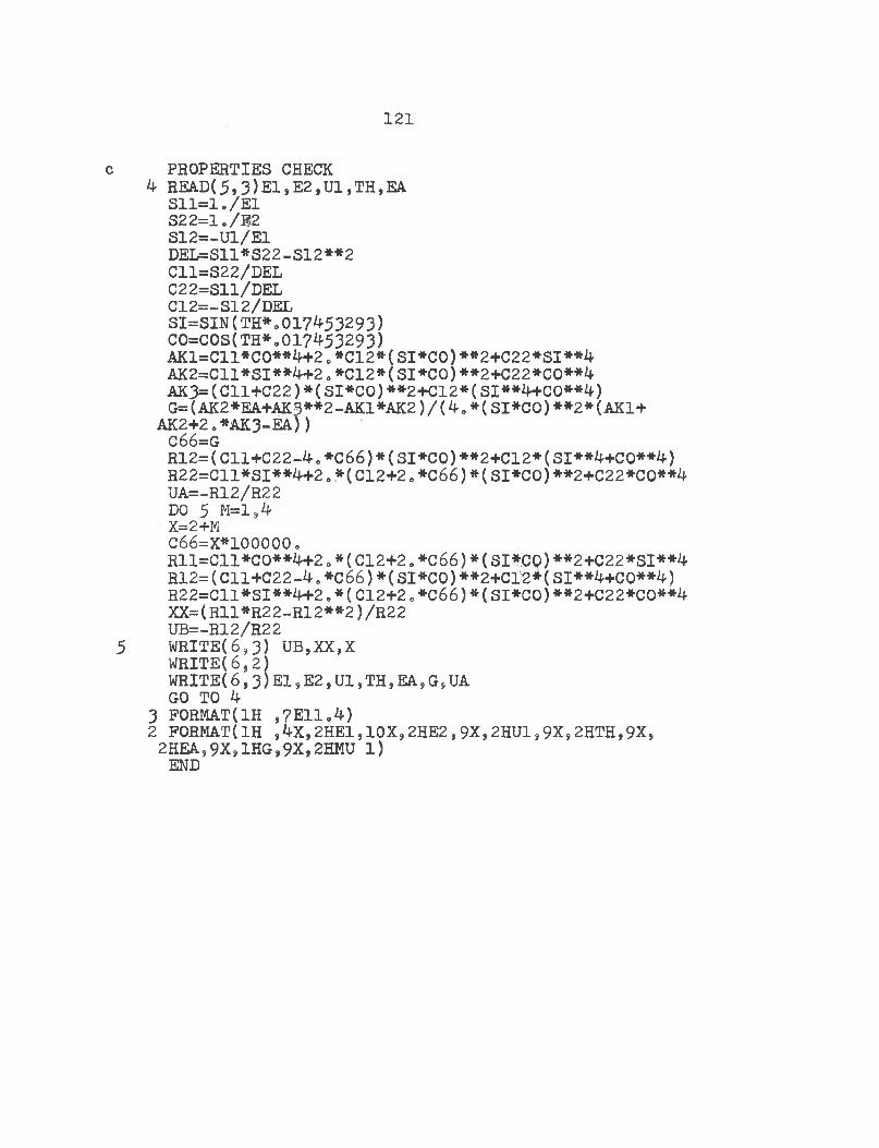
c PROPERTIES CHECK4 REA.D(5,3)E1,E2,U1,TH,EA

S11=1./E1 S2 2=1«/ F2 S12=-U1/E1 DEL=S11*S22-S12**2 C11=S22/DEL C22=S11/DEL C12=»S12/DELsi=sin(th*o017^53293) co=cos(th*.017453293)AKl=Cll*CO**4+2 o *C12*(SI*CO)**2+C22*SI**4 AK2=Cll*SI**4+2„*C12*(SI*CO)**2+C22*C0**4 AK3=(C11+C22)*(SI*CO)**2+C12*(Sl**4+C0**4)G=(AK2*EA+AK3**2-AK1*AK2)/(40*(SI*CO)**2*(AK1+ AK2+2o*AK3-EA))C66=GR12=(C11+C22-4, *C66)*(SI*CO)**2+C12*(Sl**4+C0**4) R22=Cll*SI**4+2.*(C12+2.*C66)*(SI*CO)**2+C22*C0**4UA=-R12/R22 DO 5 M=l,4 X=2+MC66=X*100000„Rll=Cll*C0**4+2.*(C12+2„*C66)*(SI*CO)**2+C22*SI**4 R12= (C11+C22-4. *C66) * (SI*CO) **2+Cl'2* (SI**4+CO**4) R22=Cll*SI**4+2.*(C12+2,*C66)*(SI*CO)**2+C22*CO**4 XX=(R11*R22-R12**2)/R22 UB=-R12/R22

5 WRITE(693) UB,XXsX WRITE(6 s 2)WRITE(6,3)E1sE2,U1,TH,EA,GsUA GO TO 4

3 FORMAT(1H ,7E11.4)2 FORMAT(1H S4X,2HE1S10X,2HE2,9X,2HU1s9XS2HTH,9XS 2HEA9 9X91HG,9Xj 2HMU 1)END

121

LITERATURE CITED

LITERATURE CITED

L e k h n i t s k i l , S . G., T h eo ry o f E l a s t i c i t y o f an A n is o t r o p ic B o d y , G a su d a r s tv e n n o e I z d a t e l* s t v o , T e k h ik o - T e o r e t ic h e s k o l L l t e r a t u r i , M askow- L e n ln g r a d , 1 9 5 0 . ( i n R u s s ia n )

H earm on, R . F . S . , An I n t r o d u c t i o n t o A p p lie d A n is o t r o p ic E l a s t i c i t y , O xford U n i v e r s i t y P r e s s ,t w :D ong, S . B . , M a t t h le s e n , R . B . , P i s t e r , K. S . , T a y lo r , R. L . , A n a ly s i s o f S t r u c t u r a l L a m in a te s ,ARL 7 6 , C o n tr a c t N o. AF 3 3 t 6 l 6 ) - 6 9 1 0 , P r o j e c t 7 0 6 3 , T ask 7 0 5 2 ^ , 1 9 6 1 .

Yi-Yuan Yu, Application of Variational Equation of Motion To The Nonlinear Vibration Analysis Homogeneous and Layered Plates and Shells.AF^f^SJ-Vte----- -------------------Hearmon, R. F . S.» The Frequency of Flexural Vibration of Rectangular Orthotropic Plates With Clamped or Supported Edges. Journal of Applied Mech­anics, December 1959» PP 37-5 0<>Timoshenko, S.and Goodier, J. N., Theory of Elas­ticity. McGraw-Hill Book Company, Inc.,1951.Ritz, W., Theorle der Transversalschwlngungenelner Quadratisohen Platten mlt frelcn Randern. Annalen der Physik. Vierte Folge, vol 2 8 , 1 9 09s PP 7 3 7 - 7 8 6 . (in German)Young, D. Vibration of Rectangular Plates by the Rltz Method, Journal of Applied Mechanics, December,rm:----B a r to n , M. V . , V ib r a t io n o f R e c ta n g u la r and Skew C a n t i l e v e r P l a t e s R e p r e s e n t in g i d e a l i z e d M i s s i l e F i n s , CM -570, DRL-2 2 2 , U T X -l-A A -3 , D ecem b er, 1 9 ^ 9 .

Kantorovich and Krylov, Approximate Methods of Higher Analysis, Trans. Curtis D. Benster, Inter- science Publishers, 1958

1.

2.

3.

4.

5.

6.

7.

8.

9»

10.

11.

12.

13.

124

IBM 704q/7044 Operating System(l6/32K) Fortran IV Language. IBM Corporation, Programming Systems Publications, 19&3®Davis, J. W. and Zurkowski, N. R., Put the Strength and Stiffness Where You Need It., Minnesota Mining and Manufacturing Company Report T-STDB(101o05)R°I.B.M. Share, Programs SDA-M3053 and SDA-M3098.

ABSTRACT

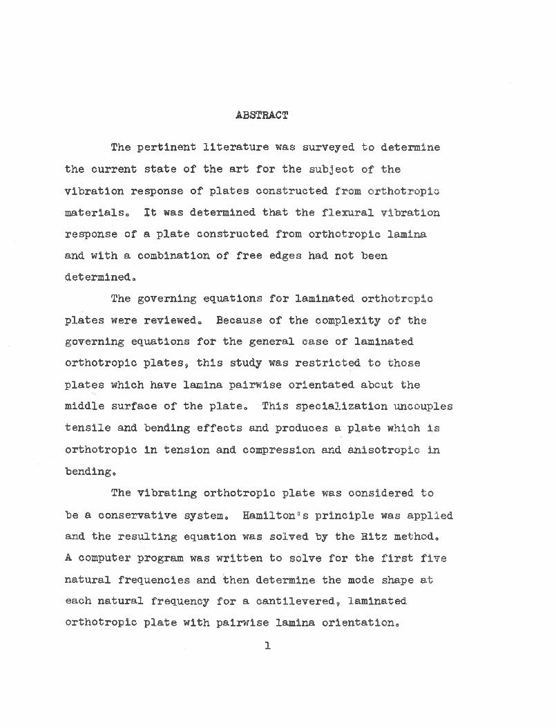
ABSTRACT

The pertinent literature was surveyed to determine the current state of the art for the subject of the vibration response of plates constructed from orthotropic materialso It was determined that the flexural vibration response of a plate constructed from orthotropic lamina and with a combination of free edges had not been determined.

The governing equations for laminated orthotropic plates were reviewed. Because of the complexity of the governing equations for the general case of laminated orthotropic plates9 this study was restricted to those plates which have lamina pairwise orientated about the middle surface of the plate. This specialization uncouples tensile and bending effects and produces a plate which Is orthotropic in tension and compression and anisotropic In bending.

The vibrating orthotropic plate was considered to be a conservative system. Hamilton0s principle was applied and the resulting equation was solved by the Ritz method.A computer program was written to solve for the first five natural frequencies and then determine the mode shape at each natural frequency for a cantilevered^ laminated orthotropic plate with pairwise lamina orientation.

1

Laminated plates, constructed from fiberglass reinforced epoxy resin were manufactured for seven different pairwise orientations. The primary elastic properties of the fiberglass reinforced epoxy resin were determined. Using the primary elastic properties, the analytical flexural vibration response of each plate was determined and then correlated with the experimental flexural vibration response.

Recommendations were made for future research on the vibration response of laminated orthotropic plates.

APPROVED?

2