The Vertical City: Rent Gradients and Spatial Structure

Crocker H. Liu Robert A. Beck Professor of Hospitality Financial Management

School of Hotel Administration Cornell University

Phone: (607) 255-3739 chl62@cornell.edu

Stuart S. Rosenthal

Maxwell Advisory Board Professor of Economics Department of Economics and Center for Policy Research

Syracuse University Syracuse, New York, 13244-1020 Phone: (315) 443-3809

ssrosent@maxwell.syr.edu

William C. Strange RioCan Real Estate Investment Trust

Professor of Real Estate and Urban Economics Rotman School of Management

University of Toronto, Toronto Ontario M5S 3E6, Canada Phone: (416) 978-1949

wstrange@rotman.utoronto.ca

June 6, 2015

Version: February 8, 2016

PRELIMINARY: COMMENTS WELCOME

We thank Laurent Gobillon and Anthony Yezer for helpful comments, as well as seminar participants at George Washington University and the Federal Reserve and attendees at presentations at the 2015 UEA/NARSC Conference in Portland and the AREUEA Annual Meetings in San Francisco. We also thank Daniel Peek and Joseph Shaw for valuable discussions on commercial buildings and leases. In addition, we thank several commercial real estate organizations for providing us with access to their offering memoranda. CompStak data were obtained with support from the Center for Real Estate and Finance at the School of Hotel Administration at Cornell and also from the Maxwell School at Syracuse University. Strange acknowledges financial support from the Social Sciences and Humanities Research Council of Canada and the Centre for Real Estate at the Rotman School of Management. Nuno Mota, Sherry Zhang, Jindong Pang, and Boqian Jiang provided excellent research assistance. Errors, of course, are the responsibility of the three authors.

Abstract

We model vertical spatial structure in tall commercial buildings that dominate city skylines. Tension between street access and height-based amenities causes access-oriented and amenity-oriented establishments to sort vertically. Unique data is used to confirm model predictions. We find a ground floor rent premium (up to 50%) followed by rising rents; street level retail followed by high-productivity offices sorting further up than low-productivity offices; and within-building employment impacting rent more than employment outside the building. These patterns are empirically important: moving up one floor, for example, increases rent by an amount equivalent to adding 2,500 workers to a building’s neighborhood.

JEL Codes: R00 (General Urban, Rural, and Real Estate Economics), R33 (Nonagricultural and Nonresidential Real Estate Markets) Key Words: commercial real estate, access, amenities, spatial structure, rent gradient, vertical.

I. Introduction

Cities, like the world itself, are not flat, but urban and real estate economists have often treated

them as if they were. This is an important omission. Cities are defined by the tall buildings that make up

their skylines, and their economies are dominated by the office activities that these buildings host. To

take one famous example, the World Trade Center’s twin towers in total had roughly 50,000 workers in

10 million square feet of space, making each equivalent in scale to a small town.1 And the differentiation

within such tall buildings probably exceeds what one might see in a small town. Within a tall building

there are prestigious and downmarket “neighborhoods.” There are educated workers engaged in a range

of high-value production activities and uneducated workers who carry out more routine activities. There

are also infrastructure issues analogous to those facing a city, such as the management of the building’s

elevators. In other words, tall buildings are like small cities in composition as well as in scale. And tall

buildings are increasingly important, with recent years witnessing a renewed burst of skyscraper

construction worldwide.2 Despite this and the great complexity of the economic activity taking place

within tall buildings, economists have typically paid little attention to what takes place inside tall

buildings, effectively treating these buildings as black boxes.

This paper will begin to fill in this gap by considering vertical spatial structure. It builds on the

standard urban model of Alonso (1964), Mills(1967), and Muth (1969), with its analysis of general

equilibrium in a monocentric setting. This has been the workhorse model in urban economics, generating

important insights regarding how the interactions among markets govern the nature of cities. The

monocentric model also is fundamental for real estate, explaining in a precise way the aspects of location

that impact real estate prices. This model has only a crude treatment of verticality, however. It allows the

production of residential space to employ variable capital to land ratios. This translates directly into

building height. It is typically assumed that capital prices do not vary with space. This means that the

capital-to-land ratio and building height both vary inversely with distance to the exogenous city center. In

these treatments, all activity at a particular distance from the city center is treated as taking place at

ground level. In other words, the standard model ignores what takes place within a building at a

particular location, and in that sense treats the world as flat.

This paper’s analysis is guided by a theoretical model that extends standard economic analysis by

considering verticality. Specifically, the buildings are each literally “long narrow cities” in the sense of

Solow and Vickrey (1971). The vertical transportation costs that motivate our research are quantitatively

1 See https://www.nysm.nysed.gov/wtc/about/facts.html. 2 The burst in construction has included several successive tallest buildings in the world (Petronas Towers, Taipei 101, and Burj Khalifa. There has also been a skyscraper boom in New York, as well as in other North American cities. See Economist (2015) and http://www.nationalgeographic.com/new-york-city-skyline-tallest-midtown-manhattan/ .

2

important relative to the more traditional horizontal transportation costs at the heart of the Solow-Vickrey

analysis. Census data indicate average one way commutes of 24 minutes (Rosenthal and Strange, 2011).

Calculations based on an IBM (2010) survey of office tenants show a typical tenant spending 22.36

minutes in elevators in a business day. In addition to being unique in considering vertical transportation,

the paper’s analysis is also unique in providing a spatial model of commercial real estate markets. These

commercial markets are vast, larger than the market for corporate bonds. While there is an extensive

financial literature on commercial real estate, focusing on Real Estate Investment Trusts REITS), there

has been very little research on the spatial nature of these markets. The model generates predictions about

both the vertical rent gradient and vertical spatial structure.

The model’s predictions are then tested. We make use of three unique data sources, two of which

have only recently become available. First, we make use of a set of confidential offering memoranda

(OM) that lay out the tenant stack (tenant locations) and rents by floor for 93 tall buildings spread across

18 metropolitan areas. Second, we make use of a new commercial rent dataset produced by CompStak

Inc. (CS). These data report rents and occupancy for a largely random set of tenants within buildings

spread across portions of seven metropolitan areas. Third, we employ establishment-level Dun and

Bradstreet data (D&B). Although D&B does not report rents, it does report floor number and a wide

range of firm and establishment characteristics that help us to understand sorting patterns within tall

buildings in response to vertical amenities that make high locations attractive despite inferior access. In

some applications we match the D&B data at the tenant level with occupants of the OM buildings. In

other instances we match building-level and zipcode-level employment from D&B and Census to

individual tenants in the CS data. In still other extensions we develop a separate D&B-only database

drawn from 12 metropolitan areas to examine systematic vertical patterns of labor productivity (based on

sales per worker) for law offices and other common industries in tall buildings.

The empirical analysis reaches a number of important conclusions. The first is that verticality

matters. Both pricing and spatial structure vary vertically in ways that standard urban models fail to

capture. Second, the vertical rent gradient is non-monotonic. Rents initially decrease sharply as one

moves above the ground floor and access worsens. In other words, there is a ground floor premium.

Above the second floor, however, rents rise as some sort of amenity outweighs the growing adverse

access effect. This amenity is more complicated for the commercial markets that we consider than it

would be in a residential setting. For the latter, it is easy to believe that residents value the views that

high floors create. See, for instance, Pollard (1980, 1982), and the literature on the hedonics of views that

follows.3 In a commercial setting, however, rents can rise as access deteriorates only if profit rises as one

3 See Sirmans et al (2005) for a review of the broader hedonic literature in which the view literature resides. Rodriguez and Sirmans (1994) exemplifies this line of research, one that is entirely residential. The implications of

3

moves higher in the building. We will argue below that this can occur if workers view height in the

building as a workplace amenity. It can also arise through signaling that may help to attract talented

workers or convince clients of service quality.

The magnitudes of these effects are substantial. Moving up from the ground floor to the second

floor, rents drop roughly 50% depending on the model and sample. Moving up from the second floor

causes rent to increase by roughly 0.6 percent per floor with a steeper rent gradient high up off the ground

(e.g. above floor forty). It is worth emphasizing that the magnitudes of these estimates differ across

individual buildings and appear to vary systematically with building height and other features of the

building and location. However, the core qualitative pattern is robust: a sharp ground floor premium with

rents rising above the second floor at an increasing rate.

The paper’s third main conclusion derives from these magnitude calculations. In models where

we added zipcode-level employment and within-building employment to our rent models, we find a

stronger relationship between rent and building employment than with employment in the building’s

zipcode. More precisely, the effect of within-building employment is more than three times larger than

the effect of zipcode employment. To put the various estimates in context, adding 2,500 workers to a

building’s zipcode increases rent by an amount about equal to moving up one floor. While this paper is

not primarily concerned with agglomeration, these results are consistent with agglomeration economies

that attenuate with distance, echoing findings in Rosenthal and Strange (2003, 2004, 2005, 2008, and

2012) and Arzaghi and Henderson (2008). Moreover, adding employment to the rent models has almost

no effect on the estimated vertical rent pattern and vice versa. This means that both traditional

“horizontal” measures of nearby economic activity as well as vertical location have important effects on

commercial rent. Our findings also suggest that these effects are largely independent of each other.

The paper’s fourth main conclusion follows naturally from the vertical rent pattern: vertical

spatial structure is determined by tension between access and amenities. There are many manifestations

of this. For instance, access-oriented retailers tend to occupy the lowest floors of tall buildings, while

amenity-oriented office uses occupy higher floors. Within the office category, some activities are

consistently found high in the building, while others are not. Law firms, for instance, are frequently

found on high floors. More generally, establishments that display high labor productivity, in the sense

that sales-per-worker is high conditional on employment at the site, tend to be higher. This result is

consistent with high productivity workers valuing view amenities to an especially great degree, which

amenities related to building height in a commercial setting have not been considered at all, and the issues are different in important ways. The broader issue of vertical transportation costs has also been considered in a limited way within urban economics. Sullivan (1991) shows how tall buildings can make sense even on cheap land when the advantages of vertical transportation are great, as they are, for instance, with elderly households. This is also a residential paper.

4

would be the case if view amenities were a normal good. Furthermore, we also find that establishments

with high employment also locate on high floors. All of these results are robust to inclusion of MSA

fixed effects, zipcode fixed effects, or building fixed effects. Overall, we tend to observe establishments

that are in some sense high fliers to locate towards the top of the buildings in our samples.4

The paper builds on several lines of research. The first concerns the theory of urban spatial

structure. See Brueckner (1987) and Duranton and Puga (2015) for insightful surveys of the research that

followed the initial contributions of Alonso-Muth-Mills. The long narrow city paper of Solow and

Vickrey (1971) is one particularly relevant paper, since with tall buildings, the long-narrow assumption

holds exactly, in contrast to actual cities. There have been few papers that have considered vertical

structure. Urban historians, see Glaeser (2011) or Bernard (2014) for instance, have noted that prior to

the elevator, residential buildings were typically under six stories, with the top occupied by the lowest

income tenants. Elevators were crucial to the development of modern cities because they allowed

increases in density. While this is presumably because they have increased accessibility, this literature

does not examine what takes place within a building. Our contribution here is to carry out this

examination.

The second line of research concerns the empirics of urban spatial structure. As noted by

Duranton and Puga (2015), much of the empirical research assessing the predictions of the monocentric

model has been carried out at an aggregate level despite the model offering strong predictions at the

individual property level. The analysis here is micro. With regard to both the empirical and theoretical

literatures, the paper breaks new ground in its focus on the spatial structure and pricing for commercial

real estate. The prior literature has instead focused almost entirely on residential issues. Ahlfeldt et al

(2015) is a notable exception, focusing on spatial interactions between households and their employers.

Finally, by focusing on within building variation, the paper avoids some of the pitfalls noted by Duranton

and Puga for estimation of residential models. In particular, in this setting we do not have the omitted

variable problems that have plagued estimates of residential rent gradients. We also do not face the

difficulty associated with defining the employment center; within a building, the first floor naturally plays

a central role. This paper’s analysis is thus a particularly clean treatment of the crucial issue of spatial

equilibrium.

The third line of related research concerns commercial real estate. As noted above, commercial

real estate is a very important asset class, but it has perhaps received less academic attention than it has

merited. There is a well-established financial literature on commercial real estate. There is a tendency in

this literature to take rents as primitive and then compute asset values, financial structures, or asset 4 The most high-performing such tenants are often referred to in the real estate industry as “trophy” or “anchor” tenants. In the specific case of retail tenants, the term “anchor” refers more narrowly to large tenants who generate externalities for others.

5

allocations based on these primitive prices (see, for instance, the textbook by Geltner et al, 2007). One

line of economic research has focused on the valuation of buildings. Colwell et al (1988) estimates a

relationship between building price and height. Shilton and Zaccaria (1994) is another paper in this

tradition. Another line of research has considered commercial leasing. Grenadier (1995) considers

decision to lease in particular, exploring in particular the option issues that arise out of the dynamics of

the leasing decision. Wheaton and Torto (1988) consider the macroeconomic dynamics of office markets.

Finally, other related literature has examined retail malls, focusing on the role of anchor tenants.

Brueckner (1993) provides a seminal model of the incentive issues. Konishi and Sandfort (2003) present

a newer model with a search structure that also considers anchor tenants. Gould and Pashigian (1998) and

Gould, Pashigian, and Pendergast (2005) carry out an empirical survey of these and related issues. With

respect to the present paper, prior work on commercial real estate has only lightly touched on spatial

issues – they are mentioned in some of the papers on malls – and has not touched at all on vertical issues.

Our paper, therefore, fills a large hole in the understanding of one of the crucial markets in a city’s

economy.

Finally, the fourth line of relevant research concerns building height. This literature combines

elements of the three lines of research described above. On the theory side, Helsley and Strange (2008)

present a game theoretic model where builders derive payoffs from having a tall building independently

of the rents that might accrue. On the empirical side, Barr (2010, 2014) carefully documents the patterns

of building heights in Manhattan and analyzing the forces at work. More recently, Koster et al (2014a)

employ rich data from the Netherlands to consider the relationship of office rents to building heights.

They obtain the result an office in a taller building will command a greater rent, which they show can

reflect views or the landmark nature of tall structures. Ahlfeldt and McMillan (2015) document a robust

relationship between building heights and land rents using Chicago microdata that spans more than a

century. In addition, their paper shows that the spatial dispersion of tall buildings can be explained by the

dissipative competition for height modeled by Helsley and Strange.5 These papers are notable as papers

that move beyond the flat earth approaches of classic urban economics. The present paper is distinct from

them by virtue of the microdata that we have assembled, allowing us to look within buildings in ways that

have not been possible using previous data.6

The remainder of the paper will be organized as follows. Section II presents a theoretical model

laying out some of the microfoundations of commercial markets and presenting some predictions that will

be confronted with data. Section III describes the unique data that have gone into this paper’s analysis.

5The present paper and Alfeldt-McMillen (2015)were both submitted in June 2015 for consideration for presentation at the Urban Economic Association 2015 meetings. Neither author team was aware of the other’s work. The similarity in titles was accidental. 6 Koster et al (2014a) have some observations of an office suite’s floor in their data, but fewer than 100.

6

Section IV computes vertical rent gradients, while Section V presents results on which tenants locate

where. Section VI concludes.

II. A theory of vertical bid rent and spatial structure

This section lays out a theory of the vertical allocation of activities to commercial space. The

demand structure is stylized, with rents depending on two factors: access to the ground floor and

amenities that rise (in some situations) with height off the ground. As noted above, the concept of

amenities is quite different for the commercial space that we consider here than for residential space. We

cannot simply borrow from the more developed residential amenities literature, and so we will develop

more precisely below the way that height can contribute to profit. The section will proceed incrementally,

beginning with the vertical bid rent of the retail tenants of one building. These tenants are assumed to

care only about access. We then move on to consider office tenants who care about both access and

amenities. We then consider both sorts simultaneously. The model generates a number of predictions

that will be the basis of the empirical analysis that comprises the remainder of the paper.

A. Retail activities

Consider a building with a large pool of potential retail tenants. In this “open” framework,

potential tenants bid for locations. Each tenant consumes a fixed amount of space, s, normalized to unity.

Each tenant employs a fixed number of workers, n, also normalized to unity. These and other simplifying

assumptions are relaxed later in the section.

Successful bidders serve a pool of customers of size M, who appear at the ground floor of the

building. Each tenant has the potential to serve a share of these customers. A given customer may buy

from multiple tenants, for instance shoes and a shirt. Supposing that customers are matched with

particular tenants is a convenient way to capture this sort of matching.7 A customer’s gross utility from a

purchase is v. The customer incurs two sorts of cost, a price p that is set by the retailer and the vertical

transport costs associated with the trip from the ground floor to another part of the building. Let the

retailer be located on floor z. Then transport costs associated with buying from the retailer equal Rz.

The customer will buy from each retailer with which there is a match provided the total costs incurred,

both price and access costs, are sufficiently low relative to the utility generated from a purchase.

The retailer incurs three sorts of costs, labor, rent, and other costs. For retailers, we will simply

suppose labor costs equal a fixed retail wage wR for its one unit of labor. A retailer incurs marginal cost

7 It is worth pointing out that spatial competition among tenants in the spirit of Hotelling is a much less tractable model. Since this section’s model is meant to illustrate the roles of access and amenities, we have opted for tractability.

7

of c for each customer it serves. The total rent on floor z is sr(z), which equals r(z) with the normalization

s = 1.

A retailer located on floor z chooses price to maximize its profits. In this setup, retailer profit

equals

(z) = (p-c)m(z,p) – wR – r(z), (II.1)

where m(z,p) gives the number of consumers served on floor z at a price of p. If p ≤ v - Rz, then the

tenant serves its share of customers, m(z,p) = M. In this region, the profit-maximizing price would be p

= v - Rz. If p > v - Rz, the firm serves zero customers, m(z,p) = 0, because the customers are deterred

from buying the good by its price. Taking rent and labor costs as fixed for now, the retailer will choose to

serve its customers when p = v - Rz ≥ c.

In this setup, the retailer reduces price at higher floors to keep from losing customers. It extracts

the entire surplus from the transaction. The retailer then serves its full share of customers, M, as long as

it is capable of earning non-negative profit by doing so. Profit may be re-written as,

(z) = (v - Rz-c)M – wR – r(z). (II.2)

As usual, in an open model of this sort, bidding among potential tenants results in rent adjusting to give

zero profit. The retailer bid-rent is thus

r(z) = M(v - Rz-c)– wR. (II.3)

There are two features of retail bid rent that are important for our purposes. First, retailer bid-rent

is negatively sloped,

∂r/∂z = -MR < 0 (II.4)

Rent falls as one moves to upper floors because the product becomes less accessible and thus less

attractive to consumers, resulting in a reduction in price. Other specifications of demand would lead to a

similar conclusion. For instance, if consumers differed in the utility that they received from purchase,

then the firm would trade-off price and quantity as usual. Higher locations would offer a less favorable

tradeoff, leading to the reduction in rent. The negative slope discussed here depends crucially on the

8

assumption that amenities are typically not important for retailers. We believe this to be correct most of

the time. One notable exception is high floor restaurants, where the view is bundled with the meal, and

customers may be willing to pay more at higher floors. The analysis in the next subsection can be

employed to capture this.

The second key feature of retail bid rent is that at a sufficiently high location, retail-bid rent

becomes negative. Setting r(z) from (II.3) equal to zero, gives

z* = [M(v -c)– wR]/MR. (II.5)

When access is sufficiently poor, retailers cannot make competitive bids for space. Retailers will not,

therefore, occupy this space.

We now turn to the office tenants who can make positive bids for these higher floors.

B. Office activities

Suppose the demand structure for office activities is parallel to the structure for retail activities.

Specifically, there is a pool of customers at street level of size N. Customers incur access costs, denoted

O. As above, an office tenant will serve a share of these customers as long as its price is less than or

equal to the gross utility from the purchase, pO ≤ v - Oz.8

There are two important differences between the demands for office and retail. First, the costs of

accessing the higher floors are lower for office transactions than for retail transactions. Let O denote

vertical transport costs in the office sector, with O R. The assumption that vertical transport costs in

retail are high reflects that these trips are typically taken with a slow model of travel such as stairs or an

escalator. Office trips are typically taken with a fast mode, such as elevators. Finally, it may take fewer

trips by the customer to create value. For instance, Ascher (2011) suggests that this is true for law offices.

Any of these will result in the ranking we have assumed for vertical transportation costs. This ranking

will generate a sharp empirical prediction, one that will be tested later in the paper. 9

The second difference between office and retail tenants is that some valuable “amenity” may

accrue to the tenant from its high location. In the case of a residential high-rise, the amenity is easy to

8 It is straightforward to consider differences in utility, v, between retail and office customers. This will not affect the slope of bid rent, but it will affect the level. 9 We have ignored the fixed costs of taking an elevator and the related decision of whether to walk between floors or take an elevator. In our model, the assumption that vertical transport costs for retail are higher than for office should be interpreted as capturing the willingness of customers to walk a few floors even at high cost in the presence of fixed costs for the low per-floor technology of the elevator.

9

understand. Views are better and noise is minimized at high levels. In addition, there may be prestige

associated with high locations. These effects result in a high-floor premium in residential buildings.

The role of amenities, broadly conceived, is more complicated in commercial real estate. One

possibility is that the consumers of the firm’s output value the output more if it is purchased on a high

floor. It is difficult to believe that this can account for a large enough increase in revenues to generate the

patterns discussed in the Introduction and that will be explicated in detail below. A more plausible

explanation is that there is signaling. Signaling has been offered as an explanation for various corporate

activities, including the issuance of dividends, the provision of CEO mansions, and the purchase of lavish

office space.10 The heart of the signaling argument here would be that occupying a high floor indicates

unobservable elements of the value of service to customers, resulting in greater revenue at high floors.

Yet another amenity effect operates through the labor market. While customers are likely to

spend little time enjoying the view from a high floor office that they visit, employees spend considerable

time in their offices. An office with a commanding view is an important and visible perquisite, one that is

likely to be valued by employees. This is especially so since many classes of office workers have high

incomes, which is likely to raise the value they would assign to a “perk” such as a view. In this situation,

workers will accept lower wages, raising profit. This, in turn, will raise bid-rents for high floor offices.11

We capture these various amenity effects as follows. First, we suppose that revenue rises with

floor height (the first two effects). For simplicity, we suppose that the profit function is linearly

separable, with the additional revenue equal to z. Second, we suppose that worker utility rises by z,

resulting in an equal reduction in labor costs.

In this specification, an office firm’s profit equals

(z) = N(v - Oz-c) + z – (wO- z) – r(z), (II.6)

where wO is the wage required for an office worker on the first floor, consequently enjoying no amenities.

Competition among office tenants gives the office bid rent as:

r(z) = N(v - Oz-c) + z – (wO - z) (II.7)

In contrast to the bid-rent for retailers, the office bid rent is of indeterminate slope:

10 Miller and Rock, (1985) is a seminal reference on dividends as signal. 11See for example, Rajan and Wulf (2006) for a discussion how perks can be an important element of the utility derived from compensation and thus be used to motivate far more cost-effectively than equivalent amounts of cash.

10

∂r/∂z = -NO + + (II.8)

Absent a strong enough amenity effect of some sort, bid-rent will fall as floor height rises, as with

retailers. The presence of a positively sloped bid-rent – as discussed in the Introduction -- suggests the

presence of some sort of amenity.

C. Vertical spatial structure

In this section there are two types of tenant. Retailers are access oriented, while office employers

can be amenity oriented, supposing that the amenity effects on profit are strong enough to outweigh the

negative effects on access of moving higher up in a building. In any case, the lower level of vertical

transportation costs will tend to give office tenants a comparatively strongly orientation to amenities and a

comparatively weaker orientation to access.

The equilibrium vertical allocation of space within a building to competing potential tenants will

be determined, as in the horizontal models in the Alonso-Mills-Muth tradition, by bid rents.12 In the

empirical analysis to follow, we will allow for a range of differences in access and amenity orientation.

Our purpose here is to illustrate the forces at work, and we can do that in a model that has two sorts of

potential tenants, one access oriented retailer and one amenity oriented office tenant. The office tenant’s

amenity orientation is such that the bid rent is positively sloped (see equation (II.8)).

The relative positions of the two tenant types depend on the slopes of the bid rent curve.

Retailers have a negative slope, while office firms have a positive slope. It is therefore unambiguous that

office firms will occupy higher floors and retailers will occupy lower floors, provided that both types are

present. A necessary condition for the retailers to be present is that the retailers have a positive bid rent

for the bottom floor (z = 0) and can outbid the offices there. A necessary condition for the office firms to

be present is that they have a positive bid rent for the top floor (z = Z) and can outbid the retailers at the

top of the building. These require, respectively, that

M(v -c)– wR > N(v - c) – wO (II.9)

and

N(v - OZ-c) + Z– (wO - z) > M(v - RZ-c)– wR. (II.10)

12 It is worth reiterating that the paper has followed the structure of traditional monocentric models by supposing that access to a particular location is inherently valuable. In a follow-up paper, we will consider agglomeration effects that operate within buildings.

11

(II.9) will hold if retail demand, M, is large enough relative to office demand, N. (II.10) will hold if

the difference in access costs is large, R-O, and amenities are valuable either to customers or as a signal,

, or to workers, . These conditions will give a building divided into retailers below and office tenants

above.

In reality, there is obviously a much finer gradation of tenants according to their access and

amenities orientation. Tenants with greater access orientation will tend to be lower in the building, while

those with greater amenities orientation will tend to be higher. This is an important extension of the

classic analysis of urban spatial structure. To the extent that firms do indeed differ in their access and

amenities orientations, then we will not see the same land use at a particular point in a business district.

Instead, we will see the point used in various activities at different heights.

The following are the key implications of this section’s theory:

(i) The vertical rent gradient will be non-monotonic, falling with height at the lowest floors,

and later rising at the highest.

(ii) Retail tenants will occupy the lowest floors, while office tenants will occupy the highest.

(iii) The specific patterns of occupation will depend on amenities and access orientation, with

a weaker access orientation and a stronger amenities orientation being associated with the

occupancy of a higher floor

As noted above, firms will tend to have a stronger amenity-orientation when the view is somehow more

valuable to either to their workers or their customers, possibly as a signal. In both cases, one would

expect to see high productivity or sales firms located on higher floors. In a signaling equilibrium, high

type firms signal their type by locating high. In the case of workers and amenities, high productivity

workers will tend to value amenities more highly. Taken as a group, the three implications all mean that

verticality matters, both in pricing and spatial structure.

12

D. Extensions

The model has been specified parsimoniously to allow us to illustrate how the tension between

amenity and access orientation governs vertical sorting in buildings and the accompanying equilibrium

rent relationship. This section will sketch some extensions that bear on the empirical analysis to follow.

The first concerns the horizontal structure of cities. This is the subject of traditional monocentric

analysis. Our model extends easily to incorporate this. Suppose that x gives the distance to the

predetermined center of the city. At greater distances, buildings have less floor level retail and office

demand. This can be captured by making the demand variables functions of x. If M(x) and N(x) decline

in x, then we will have the result that bid rents for both retail and office tenants decline with horizontal

distance.

The second concerns the “captive” retail demand that comes from other tenants in the building. If

M depends on building height, then it is immediate that retail rents will be larger at the bottom of tall

buildings and that retail will be a more competitive bidder for space, ultimately occupying more floors in

equilibrium. Since buildings will tend to be taller near the city center when rents are higher, captive

demand and horizontal structure will tend to work in the same direction.

The third concerns the management of the building. This is more complicated, suggesting the

possibility of the allocation of space depending on non-Walrasian forces that are absent from standard bid

rent analysis. See Han and Strange (2015) for a survey of search models for housing, and see Grenadier

(1995) for a rare instance of a non-Walrasian model of space for the commercial sector. The issue is that

a landlord may not simply allocate space to the highest bidder if the discounted expected value of another

bidder’s payments would be greater over the duration of the contract. For instance, a tenant who offers

high rent but also has a high likelihood of default will not be preferred to one who offers almost as much

rent but has a very low default probability. This sort of calculation is likely to be most important at the

top of a building, where rents are highest.

These extensions suggest an additional three predictions that can be empirically tested:

(iv) Rents will be higher in dense central locations.

(v) Rents will depend on building height.

(vi) Tenant risk will impact the allocation of space.

We now turn to the empirical analysis of these and the previously mentioned issues.

13

III. Data

A. Three primary data sources

The data for this paper are unique and open up a new set of opportunities for research on the

spatial structure of cities. We draw upon three primary data sources, each of which is described in detail

below. Collectively, our data enable us to observe actual commercial rents paid, the identity and location

of establishments within a given building (known as the tenant stack), and attributes of the leases.

Our first data source is a set of the confidential offering memoranda (OM) that are made available

to prospective investors when a building is up for sale. Drawing on contacts in the real estate industry,

we obtained access to such memoranda for 93 tall buildings spread across 18 metropolitan areas in the

United States that were up for sale at various times from 2003 to 2014. The memoranda typically provide

complete detail on the tenant stack in the building – the identity and location of all tenants – along with

extensive information on the cash flows, rents, and lease arrangements associated with each tenant.

While the tenant stack is public information the rent data are confidential and we are not at liberty to

share those data.

Our second key data source is from CompStak Inc., a newly created company (as of 2012) that

collects and markets data on commercial rents, leases, and other related measures for commercial

buildings for a number of major metropolitan areas in the United States. CompStak (CS) operates in

some respects as a co-operative. Commercial leasing agents are allowed to draw a specified number of

“comps” – the lease and rent terms associated with a comparable office space – for every comp that the

agent contributes to the data base. In New York city, as an example, the CS database currently includes

information on rent terms, lease, and other related attributes for roughly 24,000 office suites spread

around the city. Most of the CS data reflect agent reports submitted since 2012 for tenants that moved

into their suites between roughly 1999 to present. The nature of the CS database is that it will grow and

become more complete over time as the networking aspects of the data encourage additional agents to

participate and also with additional turnover of office suites. We currently draw on CompStak data for

buildings in New York, Chicago, Los Angeles, Sand Diego, Atlanta, Washington DC, San Francisco, and

the San Francisco Bay Area outside of San Francisco itself. We have selected these metropolitan areas

because they offer richer data. The list of cities for which lease comparables are collected from continues

to expand and currently also includes Dallas-Fort Worth, Houston, Minneapolis, and Sacramento. Given

our focus on tall buildings in urban areas, when drawing on the CS data, we work with only buildings that

are at least 10 stories tall (CS data also includes suites in many buildings under 10 stories tall).13

13 CoStar data was also matched with portions of the CS data from Chicago and used to fill in missing suite and floor numbers in some instances.

14

The CS and OM data provide an opportunity for validation checks in addition to having different

strengths and weaknesses. Both provide detailed information on commercial office rents, leases, and the

location of tenants in a building. The OM data contain information on the complete set of tenants in a

building at a given point in time. The CS data provide information on a subset of tenants in a given

building, but thousands of buildings are represented in the database. In addition, because of the nature of

the CS data collection process tenants in the CS data are skewed towards recent arrivals, although not

exclusively so. Regarding rents, the OM data report actual rent paid at the time the offering memo was

produced, while the CS sample includes effective rent, where actual rents are adjusted to account for

various landlord concessions such as free months of rents and fitting out allowances. The OM data are

laborious to collect as it was necessary in many instances to transcribe information embedded in the

offering memo text into a machine readable form. As an example, Appendix A displays abbreviated

information regarding the tenant mix (stacking plan) from the offering memorandum for Prudential One

and Two in Chicago with the rent information removed. These memos were entered into the public

domain as part of a CMBS (commercial mortgage backed security) filing with the SEC (Securities and

Exchange Commission).14 Appendix B displays an example of information on rents known as the rent

roll for a portion of the building known as 999 Peachtree Street in Atlanta, Georgia which is also in the

public domain through SEC filings.15 The information on rents is similar to what is contained in our

offering memorandums, but with less detail. The 93 offering memo data used here were transcribed over

a one and one-half year period from 2013 to 2015. In contrast, the CompStak data are commercially

available and are not subject to restrictions based on confidentiality. The CompStak data also cover over

100,000 office suites spread across thousands of buildings. Not all of the CompStak records indicate

floor or suite number, however, and others contain other types of missing information. Our cleaned

CompStak file with all of the key variables present includes 37,007 suites spread across 1,922 buildings.

Our third major data source is Dun and Bradstreet (D&B), obtained through the Syracuse

University library. Rosenthal and Strange (2001, 2003, 2005, 2008, and 2012) have previously used

D&B data in a series of papers in which the data were obtained already aggregated to the 5-digit zipcode

level. Recently, Syracuse University obtained a site license with Dun and Bradstreet that permits us

(given Rosenthal’s Syracuse affiliation) to download establishment level data. These data provide

detailed information on employment and sales at an establishment’s site (i.e. suite), establishment type

(i.e. single site, branch, headquarters), corporate status (corporation, partnership, sole proprietorship), risk

attributes, sales and employment of the overall firm for multi-site companies, and many other attributes of

14http://www.secinfo.com/dsvrn.v4Mq.htm 15http://www.sec.gov/Archives/edgar/data/1031316/000117152013000210/ex10-1.htm

15

the establishments. Among these other features includes the establishment SIC code down to the 6-digit

level although in most instances we focus on 2-digit level classifications of an establishment.

Critical to our work, the D&B data also provides the complete street address of the establishment

which, in many instances, also indicates the floor number on which the establishment is located. A

limitation of the D&B data is that at most one floor number is indicated. For tenants that occupy space on

multiple floors this injects a degree of measurement error. However, we have confirmed using the

offering memo data and also CompStak that the large majority of tenants in commercial office buildings

occupy space either on a single floor or on adjacent floors. For these reasons, we do not believe that the

measurement issues regarding floor number in the D&B data are serious. In addition, as will become

apparent, we use the D&B floor number data primarily when evaluating vertical patterns of productivity

for law offices and other related service areas (e.g. financial services). These sorts of companies are

especially likely to occupy space on a single floor. Moreover, floor number in these instances is used as a

dependent variable and for that reason, classical measurement error does not bias our estimates.

In some applications we merge the D&B data at the tenant level with tenants in the 93 tall

buildings from our offering memos. This enables us to examine location within the tenant stacks by

industry SIC classification. Future extensions will also combine rent data with the employment and sales

data from D&B.

The offering memos identify tenants only based on their name while D&B identifies tenants by

name and also their unique D&B assigned DUNS number. To match OM and D&B tenant data, we

searched the web by tenant name for each of the roughly 6,000 tenants in the offering memo data and

determine their DUNS number which was then coded to the CS file and used to match with D&B records.

The match rate was close to 70 percent from among all of the tenants in the OM data, held down in part

because the D&B data to which we have access are current whereas some of the OM data reports tenants

as far back as 2003.16

In other portions of the empirical work to follow we rely solely on the D&B data for five select

industries in twelve metropolitan areas. Details on this portion of the D&B sample are provided later in

the paper. Also, census data on employment at the zipcode level for 2013 was merged with the CS data

for selected applications.

16 It is also worth noting that whereas CS and D&B emphasize accurate data on current tenants, some of our offering memos go as far back as 2003.

16

B. Summary statistics

Table 1 provides summary measures on key data from each of the three data sources described

above. In all cases here and throughout the remainder of the paper, all dollar valued variables (e.g. rents,

sales) are reported in 2014 dollars.

Panel A summarizes the size and time period of each of the databases including number of

tenants, number of buildings, number of cities or MSAs in which buildings are located, and time period

covered. Note that in the OM data 5,750 tenant-suite observations are spread across 93 buildings in 18

cities. In the CompStak data, 36,733 tenant-suite observations are spread among 1,840 buildings in the 7

metro areas covered by CS as mentioned above. These include a number of well-known buildings, such

as the Empire State Building, Trump Tower, Chrysler Building, Citigroup Center, John Hancock Center

and Willis Tower. The D&B data is matched to each of the buildings in the OM and CS data as

described above. In addition, for five select industries including law offices (SIC 81), advertising offices

(SIC 7311), brokerage offices (SIC 62), insurance carriers (SIC 63), and agents, brokers and services (SIC

64), D&B data were collected for all such establishments in 12 MSAs (New York, Chicago, San

Francisco, Los Angeles, Atlanta, Washington DC, Cleveland, Detroit, Dallas, Denver, Houston, and

Seattle). For this data file we have 57,748 tenant-suite observations spread across 19,721 buildings based

on the street addresses reported in the data.

Panel B summarizes the composition of tenants in the 93 OM buildings. Summary measures are

presented for all floors combined, ground floor and below (the concourse levels), between floors 2 and

40, and floor 40 and above. We highlight the industries that are most heavily represented in commercial

office buildings. This includes retail (SIC 52-59), FIRE (SIC 60-67), business services (SIC 73), law

offices (SIC 81), and Engineering-Accounting-Management (SIC 81).

As seen in the first column, FIRE and Law offices account for 23 percent and 20 percent,

respectively of all establishments while Engineering-Accounting-Management makes up 12 percent.

Retail is just 6.8 percent of establishments in tall commercial buildings. A quick skim of the remaining

columns, however, indicates that the composition of activity differs sharply with height off of the ground.

On the ground floor, retail accounts for near 33 percent of establishments while law offices just 2.6

percent. From floors 3 up to 40, retail is just 2.3 percent of establishments while FIRE is 25.7 percent and

law offices are 20.6 percent. Above floor 40, retail is 3.4 percent – all of which are restaurants – and

FIRE is 25.4 percent. Law offices dominate, however, and make up 43 percent of establishments above

floor 40. These patterns provide graphic evidence of spatial stratification of activity within tall office

buildings as implied by the conceptual model discussed earlier. We will return to this point later.

Panel C provides summary measures on rent per square foot in the 93 offering memo buildings

and the 1,840 buildings drawn from the CompStak data. The average rent per square foot across the OM

17

data is $38 per square foot while for the CS data average rent is $24 per square foot. These values are

broadly consistent with the residential rents for Manhattan: a recent report indicates that the average rent

per square foot for residential space in Manhattan as of January, 2013 (in $2013) was $50.71.17

Two other important patterns are also evident in Panel C. The first is that there is considerable

variation in rents across office suites. In the OM data, rents at the 25th, 50th, and 75th percentiles are $22,

$33, and $51 per square foot. For the CS data corresponding values are $3, $19, and $38 per square foot,

respectively. The second pattern to note is that the rent distributions in the OM and CS data are of similar

general magnitude, with the effective rents from the CS data slightly lower than the actual rents from the

OM data. This provides an implicit check on the coverage and quality of the two data sources, although

differences in rents across individual buildings are to be expected.

Panel D of Table 1 characterizes the distribution of building heights across the OM and CS

samples. It does this in two ways. The first two rows of Panel D report summary statistics on building

height calculated across the buildings in the sample. Here, we see that the mean height is 32.7 stories in

the OM data and 21.5 in the CS sample. The last two rows of Panel D report summary statistics

calculated by tenant suite. There are more suites in a given tall building than in a given smaller building,

and this means that the suites in the two samples tend to be drawn more heavily from taller buildings.

The means in these samples are consequently larger, at 39.5 floors for the OM sample and 30.5 floors for

the CS sample. In the OM data, 59.9% of observations are at or above floor 30, and 10.5% are at or

above floor 60. In the CS data, 47.1% of observations are at or above floor 30, while 3.9% are at or

above floor 60. Overall, the OM sample is somewhat more skewed towards more tall buildings.

Finally, Panel E reports employment for zipcodes in which CS buildings are located. Again, we

compute summary statistics in two ways, this time by zipcode and by tenant suite. Average zipcode

employment calculated by zipcode is 36,650. Calculated by tenant suite, the average rises to 85,430.

This again reflects the tendency to oversample suites from taller buildings since such buildings tend to be

located in locations with substantial employment. There is also considerable variation in employment

across our sample, with an interquartile range in the zipcode calculations of 26,390 and a larger

interquartile range when calculated by suites.

We are now able to begin reporting our results on vertical rents and spatial structure.

17See http://www.millersamuel.com/files/2013/02/Rental_0113.pdf .

18

IV. Vertical rents

A. Baseline estimates of the vertical rent gradient and ground floor premium

Table 2a reports estimates of vertical rent gradients using the OM data (in columns (1) and (2))

and the CS data (in columns(3) and (4)). These regressions control for building fixed effects, so

identification is based on within building variation in rents. For both data sources, two models are

reported. The first regresses the log of rent per square foot on log of floor number.18 The second is a log-

linear model in which floor number is entered linearly. Additional controls are included to allow for a

ground floor premium and, in the offering memo data, a concourse (below ground floor) discount. We

allow the ground floor premium to vary with building height by including an interaction term. In all

cases, rent is reported in 2014 dollars and standard errors are clustered at the building level.

In all specifications and for both datasets, there is a large, highly significant, and positive ground

floor premium. Columns (1) and (3) report results from the double-log models. In the OM data the

premium for a 30 story building is 72 percent (equal 30*0.007 + 0.5148) while in the CS data the

corresponding premium is roughly 33 percent. The below-ground coefficient for the OM data in column

(1) is small and not significant (the t-ratio is -0.25). Estimates for the log-linear models in columns (2)

and (4) are mostly similar. The ground floor premium for a 30 story building here is 61 percent for the

OM sample and 25 percent for the CS sample. On the other hand, the below ground discount is now large

and significant for the OM sample. These results suggest that the ground floor is especially valuable

relative to locations both just above and below ground level. The theoretical model suggests that these

findings reflect the value of access. Two additional remarks are in order. First, the advantages of the

ground floor may arise from other mechanisms than the one presented in Section II’s theory. In

particular, the ground floor provides greater exposure to foot traffic, which is likely to increase sales and

so profit. Second, the large ground floor premium is a consequence of very high transportation costs of

moving up or down one floor. This, in turn, results from the fixed costs of taking elevators, which lead

customers to walk or take an escalator (both slow) for a one floor trip instead of taking an elevator (fast).

There is also robust evidence of rents that rise with floor number beyond the second. In the

double log models (in columns (1) and (3)), the elasticities of rent with respect to floor number are 28.5

percent in the OM data and 8.6 percent in the CS data. In the log-linear models (columns (2) and (4)), a

one floor increase in height above the ground level increases rent by 1.73 percent in the OM data (with a

t-ratio of 2.73) and 0.6 percent in the CS data (with a t-ratio of 17.81). These estimates indicate that

despite rising access costs, rents rise with height off the ground. Coupled with the previously noted

ground floor premium, the vertical rent gradient is nonmonotonic.

18 More precisely, the key independent variable is the log of floor number + k where k is set to one unit larger in absolute value than the lowest numbered concourse floor in the data, -5 for the OM data and -1 for the CS data.

19

Table 2b explores these patterns further and demonstrates that the vertical rent gradient is steeper

higher up off the ground. In Table 2b, Panel A presents results for the double log model, while Panel B

presents results for the log-linear model. For each specification, the first three columns are based on OM

data while the second three columns are based on CS data. The samples are further stratified into three

groupings of floors with separate regressions for each: estimates for floors 3 to 29 are in columns (1) and

(4), estimates for floors 30 to 59 are in columns (2) and (5), and estimates for floors 60 and higher are in

columns (3) and (6).

The key result in Table 2b is that rents rise beyond the first floor at an increasing rate. Reading

across columns from lowest to highest floor groupings, in the double log specification, the rent elasticity

coefficients from the OM data are 0.1447, 0.1352, and 5.40, respectively (with t-statistics of 4.31, 0.81,

and 649.37).19 For the CS data, the corresponding coefficients are 0.0763, 0.2873, and 1.274 (with t-

statistics of 16.60, 7.29 and 4.20). Estimates for the log-linear model display a similar pattern. In the OM

sample, the gradients for the three bins are 0.82 percent, 0.33 percent, and 6.2 percent. In the CS sample,

the gradients are respectively 0.58 percent, 0.68 percent, and 1.61 percent. These estimates indicate that

the rent gradient is rather gentle for the low floors of buildings, but it becomes steeper higher up off the

ground.

The estimates in Tables 2 and 3 are completely new to the literature and have three immediate

implications. First, in contrast to the maintained assumption of the standard urban model, it is apparent

that there is not a single rent value at a given street address. Instead, within a typical building large,

systematic differences in rent are present as one moves up off the ground. Second, the fact that rents

increase with height once above the ground floor confirms that height-based amenities must be present

and that height-based amenities must increase at a rate sufficient to offset rising access costs. Third, the

tendency for rent gradients to be steeper on the higher floors of a tall building could reflect that height-

based amenities increase at a non-linear rate as one moves up above the obscuring effect of adjacent

buildings. However, a different mechanism also likely contributes to this pattern. A familiar result from

the standard monocentric model is that sorting across locations between heterogeneous agents with

different bid functions can impact the curvature of the equilibrium rent function, a principle that applies

here. The convex pattern of vertical rent gradients in Table 2b, therefore, could indicate that tenants who

place greater value on height sort into higher locations. We revisit this possibility later in the paper when

we consider more direct evidence of vertical sorting patterns. Before doing this, however, it is useful to

evaluate whether and in what fashion nearby agglomeration of economic activity affects commercial rents

and the vertical rent gradient.

19 It is important to note that the OM sample contains only 4 buildings above 60 stories. The high suites in these landmark buildings (all in NY or Chicago) are clearly different from other buildings in our data.

20

B. Vertical vs. horizontal rent gradients: magnitudes and agglomeration

As noted earlier, the standard monocentric model in urban economics solves for equilibrium rents

and spatial structure in a horizontal setting. Locations farther from the central business district (CBD) in

ground level distance will differ in employment, productivity, wages, and rents from locations that are

closer. Even though this literature recognizes that higher rents in locations offering superior access to the

CBD will prompt developers to use land more intensively, causing building heights to rise, the buildings

themselves are treated as if they were flat, with all employment at the ground level. This section expands

our rent regressions by adding controls for employment within a building’s zipcode and also within the

building itself. This will allow us to evaluate the relative magnitudes of vertical and horizontal rent

effects, in addition to assessing the degree to which our estimates of the vertical rent gradient may be

sensitive to nearby agglomerations of employment.

To this end, Table 3a presents a series of rent regressions that extend the specifications in Table

2a. All of the models in this table are estimated using just the CS data because this data source offers

greater geographic coverage compared to the 93 buildings in the OM data. Except where noted, building

fixed effects are also replaced with MSA fixed effects as this allows us to explore the impact of nearby

employment. Columns (1) to (4) present estimates from double-log models while columns (5) to (8)

report estimates from log-linear models. For each group, the first column (columns 1 and 5) controls only

for zipcode-level employment for the zipcode in which the building is located; the second column

(columns 2 and 6) controls for vertical location and building height but omits any control for nearby

employment; the third column (columns 3 and 7) combines controls for both zipcode-level employment

and vertical location. The models in columns (4) and (8) repeat the building fixed effect models from

Table 2a. In the present context, it is worth noting that the building fixed effects capture proximity to

nearby employment as well as proximity to other valued location specific attributes. The fixed effects

also, of course, control for unobserved attributes of the buildings themselves.

In columns (1) and (5), zipcode employment has a positive and highly significant effect on rent.

In the elasticity model (column (1)), doubling zipcode employment increases rent by roughly 10.7 percent

while the gradient in the log-linear model (column (5)) indicates that adding 1,000 workers to a zipcode

increases rent by 0.23 percent (the corresponding t-ratios are 5.4 and 7.6, respectively).

These estimates establish a core stylized fact that has been widely assumed but only rarely

demonstrated: densely developed locations cost more, resulting in sharp horizontal spatial variation in

office rents across business districts and cities. The estimates are also consistent with a large literature on

agglomeration economies that has established that spatial concentration contributes to productivity. Most

often, that literature has focused on wage effects from agglomeration. See, for instance, the surveys by

Rosenthal and Strange (2004), Combes and Gobillon (2015), and Behrens and Robert-Nicoud (2015). As

21

in Roback (1982), however, the productivity effects from agglomeration should also be reflected in higher

commercial rents. However, despite the strong theoretical foundations, few papers in the voluminous

agglomeration literature have used commercial rent as the outcome measure, and no previous paper has

looked at agglomeration economies at a highly local level using commercial rents. Our estimates of the

rent-employment relationship are, therefore, without precedent. Bearing this in mind, as a very rough

comparison, the 10.7 percent rent elasticity obtained here is larger than corresponding wage elasticities in

the literature, which typically suggest that doubling city size increases wage by 2 to 5 percent (e.g.

Rosenthal and Strange, 2004 and 2008), or by even less (Combes et al, 2008). That rents capture a

substantial share of agglomeration economies is a point made by Drennan and Kelly (2011) and Koster et

al (2014b).20

Columns (2) and (6) revisit the vertical rent regressions from Table 2a with the primary change

that building fixed effects are replaced with MSA fixed effects and building height has been added to the

specifications. The important point to note here is that the estimates are nearly identical, both

qualitatively and in magnitude, to those in columns (4) and (8) which repeat the Table 2a specifications.

The models in columns (3) and (7) combine the controls for zipcode employment and vertical

location as described above. Comparing estimates in these models to the employment-only and vertical-

only models yields a striking result. It is apparent that adding controls for vertical location has little effect

on the estimated influence of zipcode employment, and controlling for nearby employment has essentially

no effect on the vertical rent pattern. Moreover, the vertical rent coefficients are also nearly the same

when building fixed effects are included in columns (4) and (8). The building fixed effects, of course,

control zipcode employment and building height, as well as a host of unobserved local and building-

specific attributes.

The remarkable stability of estimates across the models in Table 3a suggests that the processes

that drive vertical rent patterns are in some sense different from the processes that account for the positive

impact of nearby employment and other horizontal drivers of rent. The theory in Section II emphasizes

the role of vertical access costs and height-based amenities as the drivers of systematic patterns of vertical

rents. The agglomeration literature highlighted above emphasizes the positive productivity spillovers

arising from labor market pooling, sharing of intermediate inputs, and knowledge sharing (e.g. Rosenthal

and Strange (2004)). Our estimates from Table 3a are consistent with the view that these are different and

distinct underlying mechanisms that both affect commercial rents.

It is also useful to consider the magnitudes of the estimates in Table 3a. For these purposes, we

focus on estimates in the log-linear model in column (7) which permits direct and intuitive comparisons

20These papers do not allow the computation of building level employment, which is necessary to consider the sorts of local effects examined in Table 3a.

22

of vertical and horizontal rent patterns. For a 30-story building, the ground floor premium is roughly 28.4

percent (0.0076 * 30 + 0.056). This is roughly equivalent to the estimated increase in rent associated with

moving up 39 floors (0.0073 * 39). It is also roughly equivalent to an increase in zipcode employment of

roughly 140,000 workers, about equal to the 75th percentile among office suites in our sample (see Table

1, Panel E). If instead, we add 100,000 workers to a zipcode – about the same as the inter-quartile range

for our sample of office suites – rent would increase by an amount about equal to moving up 27 floors.

These comparisons make clear that nearby employment and vertical location both have economically

important effects on rent.21

Table 3b builds on the model specifications in Table 3a. The key extension here is that zipcode-

level employment is decomposed into employment in and outside of the building. This allows us to

consider whether the intensity of activity inside a building might affect vertical rent gradients. Prior

evidence based on both arrivals of new establishments and wages (e.g., Rosenthal and Strange, 2003,

2008) suggests that agglomeration economies attenuate rapidly with geographic distance. The analogue

here would be that employment inside a building should have a larger effect on rent than employment

outside of the building. Evidence of such a pattern would reinforce the conclusion above that different

mechanisms are driving the vertical and horizontal rent patterns in Table 3a.

To control for building-level employment, we matched tenant records at the street address level to

corresponding street addresses in the Dun and Bradstreet data. D&B data were then used to determine the

level of employment within each of the buildings represented in the CS data file. The matching process

relies on city and street address because the CS data do not provide DUNS numbers for their tenants (the

DUNS number is a unique identifier for each establishment in the D&B database). This and other

features of the matching process make the matching process laborious. For that reason, we have matched

only those CS records found in New York City, the portion of Chicago located in Cook County, and the

portion of San Francisco located in San Francisco County. This leaves us with 28,374 suite observations

spread across 1,040 buildings in New York City and Chicago (roughly 63 percent of which are in New

York, 20 percent in Chicago and 17 percent in San Francisco).

Six different models are presented in Table 3b, each of which utilizes a log-linear specification as

we feel that is a more intuitive model to interpret when employment is decomposed into different parts.

Column (1) controls for just zipcode-level employment while column (2) decomposes zipcode

employment into employment outside versus inside of the building. Column (3) controls for vertical

location and building height but omits nearby employment. Columns (4) and (5) add the controls for

21 It is worth noting that if we omit the MSA fixed effects and estimate the models by OLS, the vertical rent gradient remains similar to the estimates in Table 3a while the elasticity with respect to zipcode-level employment rises to roughly 75 percent. This reflects that high employment zipcodes are mostly found in the largest cities (e.g. New York and Chicago) which tend to have higher rents.

23

building height and vertical location to the employment-only models in columns (1) and (2). Column (6)

adds building fixed effects which cause employment and building height to drop out of the model.

Two important patterns jump out from Table 3b. First, the coefficient estimates for the restricted

sample in Table 3b are quite similar to those presented for the larger sample in Table 3a, both with respect

to the influence of zipcode-level employment and vertical location.22 Second, in columns (4) and (5), it is

clear that within building employment and zipcode employment outside of the building both cause rents

to increase but the effect of within-building employment is 3-1/2 times larger. This echoes results from

Rosenthal and Strange (2003, 2004, 2005, 2008, and 2012) and Arzaghi and Henderson (2008) that

agglomeration economies tend to attenuate rapidly with distance. It is noteworthy that this pattern

persists even after controlling for building height, given that building height is positively correlated with

building-level employment.

There is, thus, a highly robust vertical rent gradient. Rents are not at all constant at a given street

address. Instead, rents are characterized by a significant ground floor premium, and an initial sharp

decline moving just above the ground floor. Moving further up within a building, rents rise gradually at

low floors and then more rapidly near the top of the building. Moreover, these patterns are economically

important and appear to be driven by mechanisms that are different from forces that cause nearby

agglomeration of employment to also have a positive and important effect on rent. The next section will

show that the activities that take place within a building are also not homogeneous, instead exhibiting a

particular spatial structure.

V. Vertical spatial structure

This section addresses two fundamental questions about vertical spatial structure. The first

question is who locates where: in other words, is there systematic sorting by tenant type into different

parts of the building (e.g. ground floor versus above)? The second question is: why? Answering these

questions will provide evidence of the underlying mechanisms that drive the rent gradients just

documented.

A. Vertical sorting

We begin by considering who locates where. Table 4 describes the vertical distribution of where

tenants are located in the OM data. Distributions are reported for all industries combined (column (1)) as

well as retail (SIC 52-59), not retail, law offices (SIC 81), business services (SIC 73), brokerages offices

(SIC 62), insurance companies (SIC 63), and insurance and brokerage agents (SIC 64). In all cases we 22 The coefficient on zipcode-level employment in column (1), for example, is 0.0024 compared to the corresponding estimate of 0.0073 in column (6) of Table 3a. The coefficient on floor number in column (3) is 0.0099 while the corresponding estimate in Table 3a (column (6)) is 0.0074.

24

focus only on tenants merged with the D&B data which provides information on the tenant’s SIC code.

For each industry we report the distribution of floor numbers as reflected in the 1st percentile, 25th

percentile, 50th percentile, 75th percentile, and 99th percentile floor number. These values are then plotted

in Figure 1a.

The plots in Figure 1 reveal a striking stratification of industries into different parts of tall

buildings. Retail is almost exclusively concentrated on the ground floor relative to non-retail. Law

offices are especially concentrated higher up off the ground as are brokerage offices. These patterns

reinforce the summary measures in Table 1c described earlier. The flavor of these patterns will also

persist throughout the paper even though these plots do not at this point control for MSA location, height

of the building, or other locational attributes.

B. Mechanisms: access and amenities

We now move to the second question. Panel B of Table 1 and Table 4 (along with Figure 1)

together provide compelling evidence that retail establishments are heavily concentrated on the ground

floor. Section II’s theory shows that access costs can explain this pattern. Retail establishments rely on

frequent interactions with customers who must travel to the establishment. In this context, total product

price to the customer includes sticker price plus access cost which increases with height off the ground.

In the absence of a positive amenity effect associated with height, retail bid-rents decline with height and

retail should sort into the ground level space as observed. In this sense, we view retail as an access-

oriented industry.

Outside of the retail sector the frequency of face-to-face office visits with clients and/or input

providers is much reduced. In addition, the value of the service provided is often much higher both in

comparison to retail and relative to access costs. If this were all that differed between retail and non-

retail, we would have a sufficient condition to ensure that non-retail would sort into locations above the

ground floor, as observed in Table 1 (Panel B) and Table 4. In such an environment, however, office

rents would have to decline in equilibrium with height off the ground to compensate non-retail

establishments for greater travel costs. This, of course, is not consistent with the positive rent gradients

documented in Tables 2, 3a, 3b, and 3c. To allow for those patterns, it must be the case that non-retail

establishments perceive height off the ground as a positive amenity sufficient to offset reduced access.

These arguments confirm a role for both access and amenities and suggest that both increase with height.

Tables 5 and 6 help to clarify how to interpret the positive amenity effect associated with higher

locations in a building. The tables report results from a series of models in which location is regressed on

tenant and site characteristics. In all cases, the tables draw exclusively on D&B data from twelve large

metropolitan areas. For reasons to be described shortly, in most models we restrict our samples to single-

25

site firms in law offices (SIC 81), advertising offices (SIC 7311), brokerage offices (SIC 62), insurance

carriers (SIC 63), and agents, brokers and services (SIC 64). In one model we instead focus exclusively

on headquarter establishments for multi-site firms. In that instance establishments are drawn from all

industries.

In both Tables 5 and 6, the two key regressors in the single-site firm models are the sales-per-

worker ratio for the site and the number of employees at the site. Both sales-per-worker and employment

are likely positive correlates with labor productivity. Conditional on employment, a higher ratio of sales-

per-worker suggests that labor is more productive. Productive establishments also tend to grow larger and

operate at a larger scale with more workers on staff. Importantly, higher productivity also likely affects

the intensity of amenity orientation. More productive establishments tend to pay higher wages. Since

amenities such as views are almost certainly normal goods, this will increase the value that the

establishment’s workers place on a location high up in the building, as in Section II. Our motivating

hypothesis is, therefore, that establishments with high sales-per-worker ratios and larger numbers of

workers will have a stronger amenity orientation and greater willingness to pay for locations up high.

This also suggests that companies with high sales-per-worker and larger numbers of employees may favor

higher locations so as to signal to prospective clients and business contacts that they are productive.

Additional controls include 1-0 dummies for whether the establishment belongs to a firm that is

publicly traded or whether the establishment is a subsidiary. Only a small fraction of firms are publicly

traded. Our maintained hypothesis is that these establishments are higher quality in some sense, possibly

rising to the level of “trophy” tenants. For related reasons we also control for subsidiary status although

our prior of how such establishments are perceived is less clear. We also include 1-0 dummies for D&B’s

assessment of risk based on high, medium, and low ratings; coefficients are reported for low and medium

risk with high-risk the omitted category. Lower risk companies may be perceived as more attractive

tenants, ceteris paribus, and for that reason be better fits for high floors. In addition, a tenant’s low-risk

status may also contribute to signaling incentives when choosing where to locate in a tall building.

It is important to note that employing these site-specific characteristics in the estimation requires

that we address the issue of multi-establishment firms. For multi-establishment firms the attribution of

sales to sites is uncertain. It is for that reason that we work primarily with single establishment firms.

Multi-establishment firms are interesting, however, so we do consider them in a limited way by

estimating a model of headquarter establishments. We obviously cannot employ the establishment-level

sales-worker ratio in these models. We instead work with the sales-per-worker ratio at the firm level

along with employment at both the firm and establishment levels. The employment variables speak to

productivity, as above.

26

Consider now column (1) of Table 5 which reports the results for headquarter establishments.

The strongest results are for firm-level sale-per-worker and employment. Larger firms have headquarters

located on higher floors, with an elasticity of 3.5%. Conditional on firm size and the other model

controls, the elasticity associated with sales-per-worker is 2.6 percent. Both of these estimates are also

highly significant (with t-ratios of 5.8 and 5.6, respectively). Other coefficient estimates in the model are

notable but not as dramatic: employment at the site has a small, negative and not significant effect;

publicly traded firms locate 10 percent higher (with a t-ratio of 3.18), and lower risk companies are also

higher. Subsidiary status has a negative and marginally significant coefficient of 0.049 (the t-ratio is

1.92), indicating that headquarters of subsidiaries are on somewhat lower floors after controlling for other

factors. Taken as a whole, the estimates in column (1) provide compelling evidence that headquarters of

higher performing companies are located higher up off the ground. It is worth emphasizing that this result

is obtained even after conditioning on the 5-digit zipcode in which a headquarter is located. This pattern

is also echoed in the single-site regressions.

Columns (2) and (3) of Table 5 report results for single-establishment firms pooling data from the

five industries noted above. The model in column (2) controls for both 2-digit industry and 5-digit

zipcode fixed effects while the model in column (3) replaces the zipcode fixed effects with building fixed

effects. The results are similar for the sales-per-worker ratio and for employment at the site. Both are

positively related to floor. The elasticities of floor number with respect to sales-per-worker are 1.5

percent in the zipcode fixed effect model and 1.6 percent in the building fixed effect model with t-ratios

of 2.2 in both cases. For employment at the site the elasticities are 3.1 in the zipcode fixed effect model

and 1.7 in the building fixed effect model (with t-ratios of 6.6 and 5.1, respectively). These results further

reinforce the idea that view amenities raise profit by making it easier to attract productive workers which

should result in lower wages.

Several other patterns in column (2) also suggest that higher performing establishments locate in

higher offices. In particular, the publicly traded dummy is positive and significant in column (2) as are

the coefficients on low and medium risk ratings. These results largely disappear, however, when we shift

from the zipcode fixed effect model in column (2) to the building fixed effect model in column (3). We

will comment further on these differences in the context of Table 6 to follow. First, however, we

comment on the industry-stratified models in columns 4-9 of Table 5.

As noted in Table 1, Panel B, law offices account for a significant fraction of office tenants in tall

buildings. Results for law offices are presented in columns (4) and (5) and are qualitatively similar to the

estimates for the pooled samples just described. The primary difference between the two sets of models is

that the magnitude of the sales-per-worker coefficients in the law-office models are larger: 4.6 percent in

the zipcode fixed effect model in column (4) and 2.3 percent in the building fixed effect model in column

27

(5). These estimates are clearly significant with t-ratios of 4.6 and 2.2, respectively. In the law office

sector, higher productivity companies as proxied by sales-per-worker and number of employees locate

higher up in their immediate zipcode and building.

Estimates for the other industries highlighted above are presented in columns (6) – (9). For these

industries only zipcode fixed effect models are presented given the much smaller sample sizes. Looking

across the columns it is evident that the results are mixed and point to differences in location and sorting

patterns across industries. The results for brokerage offices reported in column (7) are closest to those for

law offices (consistent with patterns in Table 4 and Figure 1). In column (7), notice that the elasticity of

floor number with respect to employment is 4 percent with a t-ratio of 4.6. Agents and Brokers in column

(9) display a similar though more muted result. The other coefficients on sales-per-work and employment

across the remaining industries are not significant and often rather small in magnitude. On the other hand,

the coefficients on publicly traded companies are revealing. In the case of law offices this variable is

omitted as no law offices are publicly traded. Of the remaining industries, notice that the coefficient on

publicly traded is -0.22 for advertising with a t-ratio of 2.88, and then positive 4.2, 1.3, and 0.6 for the

remaining three industries with t-ratios ranging from 2.5 to 45. We do not have a good explanation for

why publicly traded advertising establishments are located on lower floors. Nevertheless, for the other

industries the large positive, highlight significant elasticities are consistent with the view that publicly

traded companies are higher end (higher productivity) and locate higher up in tall buildings for reasons

described earlier.

Table 6 revisits the models for the pooled industries and law offices. In each case models are

presented for OLS specifications, MSA fixed effects, zipcode fixed effects, and building fixed effects.

This allows us to highlight systematic differences in patterns as the geographic nature of the controls

becomes more refined. The coefficients on sales-per-worker and employment at the site diminish in

magnitude as the fixed effects focus in on individual buildings. A similar pattern is present for the other

model controls (e.g. publicly traded, risk). It is worth recalling that the fixed effects capture the influence

of unobserved factors common to the observations associated with the fixed effect. Accordingly, the

patterns in Table 6 suggest that establishments tend to sort across locations down to the building level in a

manner that is correlated with sales-per-worker and the other model controls. This indicates that high

productivity companies tend to concentrate in select zipcodes and buildings, although the models in Table

6 do not highlight which attributes of a zipcode or building tend to attract productive companies. Further

extensions will address this issue.

28

VI. Conclusion

This paper departs from conventional urban economic analysis by considering the vertical

structure of cities. Our primary focus is on tall commercial buildings. Standard urban models have

treated these buildings as black boxes by taking the approach of telescoping all the activities that take

place at a particular street address down to ground level. We have shown that this approach misses the

variability both in rent and occupancy that exists within a building.

This vertical variation has two key dimensions. First, the vertical rent gradient is non-monotonic,

falling initially as one moves up off the ground floor but then rising above the second floor at a modest

rate that increases with height. Although rent levels increase with employment in and near a building,

nearby employment has little effect on the vertical pattern of rents within a building. Moreover,

employment within a building has a notably larger impact on rent than nearby employment outside of the

building. This result is consistent with previous literature that productivity spillovers from agglomeration

attenuate rapidly with distance. Together, the various patterns we document also suggest that the

processes that drive systematic vertical patterns of rents within buildings are different from the processes

associated with agglomeration economies.

Second, vertical spatial structure is determined by a tension between access costs (rising as one

moves up) and various sorts of amenities associated with an increase in profits for a commercial tenant

(also rising as one moves up). Specifically, we find that retail tenants, who are strongly access-oriented,

locate on low floors, while office tenants, with varying degrees of amenity orientation, locate higher.

Among office tenants, those who can be characterized as “trophy” or “anchor” tenants – based on

indictors of productivity – locate nearer the top of the building. In other words, verticality matters.

In future work, we will further consider agglomeration issues. Prior work has shown that

agglomeration economies are local, with affects that attenuate with distance. See, for instance, Rosenthal

and Strange (2001, 2003, 2005, 2008), Arzaghi and Henderson (2008), and Baum-Snow (2011). Due

primarily to data limitations, none of these papers have considered this issue within a building. This

paper’s results are consistent with rapidly attenuating effects. In ongoing research, we further investigate

this issue by considering localization effects and also the patterns of agglomeration that appear within

buildings.

29

References Ahlfeldt, G., S.J. Redding, D.M. Sturm, and N. Wolf (2015), “The Economics of Density: Evidence from

the Berlin Wall,” Econometrica 83(6), 2127-2189. Ahlfedt, G. and D. McMillen (2015), “The Vertical City: The Price of Land and the Height of Buildings

in Chicago,” Working Paper, July 2015. Alonso, W. (1964), Location and Land Use; Toward a General Theory of Land Rent. Harvard University

Press, Cambridge, MA. Arzaghi, M. and J.V. Henderson (2008). "Networking off Madison Avenue," Review of Economic

Studies, 75.4, 1011-1038. Ascher, K. (2011), The Heights: Anatomy of a Skyscraper, Penguin: New York. Barr, Jason. "Skyscrapers and the skyline: Manhattan, 1895–2004." Real Estate Economics 38.3 (2010):

567-597. Barr, Jason. "Skyscraper height." The Journal of Real Estate Finance and Economics 45.3 (2012): 723-

753. Baum-Snow, N. (2011). Urban transport expansions, employment decentralization, and the spatial scope

of agglomeration economies, Working paper. Behrens, K., and F. Robert-Nicoud (2014): “Agglomeration Theory with Heterogeneous Agents”, G.

Duranton, J. V. Henderson and W. Strange (eds), Handbook in Regional and Urban Economics, Amsterdam (Holland), Elsevier Press.

Bernard, A. (2014), Lifted: A Cultural History of the Elevator, NYU Press: New York. Brueckner, Jan K. (1993), "Inter-store externalities and space allocation in shopping centers." The Journal

of Real Estate Finance and Economics 7.1, 5-16. Brueckner, Jan K. (1987) "The structure of urban equilibria: A unified treatment of the Muth-Mills

model." in E.S. Mills (ed.), Handbook of regional and urban economics , Volume 2 , North-Holland: Amsterdam, 821-845.

Colwell, Peter F., Henry J. Munneke, and Joseph W. Trefzge (1998). "Chicago's office market: price

indices, location and time." Real Estate Economics, 26(1),83-106.

Combes, P.-P., and L. Gobillon (2014): “The Empirics of Agglomeration Economies”, G. Duranton, J. V. Henderson and W. Strange (eds), Handbook in Regional and Urban Economics, Amsterdam (Holland), Elsevier Press.

Combes, Pierre-Philippe, Gilles Duranton, and Laurent Gobillon (2008). "Spatial wage disparities:

Sorting matters!." Journal of Urban Economics 63( 2), 723-742. Drennan, Matthew P., and Hugh F. Kelly (2011). "Measuring urban agglomeration economies with office

rents." Journal of Economic Geography, 11(3),481-507.

30

Duranton, G. and D. Puga (2015). “Urban Land Use.” in Duranton, G., Henderson, J.V., and Strange, W. (Eds.), Handbook of Urban and Regional Economics, Volume 5A, Elsevier: Amsterdam, 467-560.

Economist (2015), “Towers of Babel: Is There Such a Thing as a Skyscraper Curse,” March 28. Glaeser, E. (2011). How Skyscrapers Can Save the City. Atlantic Magazine. Gould, Eric D., B. Peter Pashigian, and Canice J. Prendergast (2005), "Contracts, externalities, and

incentives in shopping malls." Review of Economics and Statistics 87.3, 411-422. Grenadier, S. R. (1995), "Valuing lease contracts a real-options approach." Journal of Financial

Economics 38.3, 297-331. Han, L.. and W. Strange (2015). “The Microstructure of Housing Markets: Search, Bargaining and

Brokerage.” in Duranton, G., Henderson, J.V., and Strange, W. (Eds.), Handbook of Urban and Regional Economics, Volume 5B, Elsevier: Amsterdam, 813-886.

Helsley, Robert W. and William C. Strange (2008), “A Game-Theoretic Analysis of Skyscrapers,”

Journal of Urban Economics 64(1), 49-64. IBM (2010), Smarter Buildings Survey: Consumers Rank There Office Buildings, manuscript. Konishi, Hideo, and Michael T. Sandfort. (2003), "Anchor stores." Journal of Urban Economics 53(3),

413-435. Koster, Hans RA, Jos van Ommeren, and Piet Rietveld (2014a). "Is the sky the limit? High-rise buildings

and office rents." Journal of Economic Geography, 14(1), 125-153. Koster, Hans RA, Jos Ommeren, and Piet Rietveld (2014b). "Agglomeration economies and productivity:

a structural estimation approach using commercial rents." Economica, 81, 63-85. Miller, M. H., & Rock, K. (1985). Dividend policy under asymmetric information. The Journal of

Finance, 40(4), 1031-1051. Mills, E.S. (1967), An aggregative model of resource allocation in a metropolitan area. Am. Econ. Rev.

Pap.Proc. 57, 197–210. Muth, R.F. (1969), Cities and Housing. University of Chicago Press, Chicago, IL. Pashigian, B. P. and E. D. Gould. (1998), "Internalizing Externalities: the Pricing of Space in Shopping

Malls 1." The Journal of Law and Economics 41.1, 115-142. Pollard, R. (1982). “View amenities, building heights, and housing supply ,” in D. Diamond and G.S.

Tolley (eds), The Economics of Urban Amenities, Academic Press: New York, 105-123. Pollard, R. (1980). Topographic amenities, building height, and the supply of urban housing. Regional

Science and Urban Economics, 10(2), 181-199. Rajan, Raghuram G., and Julie Wulf (2006). Are perks purely managerial excess? Journal of Financial

Economics, 79(1), 1–33.

31

Roback, Jennifer (1982). Wages, rents, and the quality of life. Journal of Political Economy, 90(6), 1257-

1278. Rodriguez, Mauricio, and C. F. Sirmans (1994,) "Quantifying the value of a view in single-family

housing markets." Appraisal Journal 62, 600-600. Rosenthal, S. S. and S. L. Ross (2015). “Change and Persistence in the Economic Status of

Neighborhoods and Cities.” in Duranton, G., Henderson, J.V., and Strange, W. (Eds.), Handbook of Urban and Regional Economics, Volume 5B, Elsevier: Amsterdam, 1047-1120.

Rosenthal, S. S., and W. C. Strange (2001), "The determinants of agglomeration." Journal of Urban

Economics 50.2, 191-229. Rosenthal, S. S., and W. C. Strange (2003), "Geography, industrial organization, and agglomeration."

Review of Economics and Statistics 85.2, 377-393. Rosenthal,S.S and W.C. Strange (2004), “Evidence on the Nature and Sources of Agglomeration

Economies”, in Henderson, J.V. and Thisse, J.-F. (Eds.), Handbook of Urban and Regional Economics, Volume 4, Amsterdam: Elsevier, 2119-2172.

Rosenthal, S. S., and W. C. Strange (2005), "The geography of entrepreneurship in the New York

metropolitan area." Federal Reserve Bank of New York Economic Policy Review 11.2, 29-53. Rosenthal, S. S., and W. C. Strange (2008), "The attenuation of human capital spillovers." Journal of

Urban Economics 64.2, 373-389. Rosenthal, S. S., and W. C. Strange (2012), "Female entrepreneurship, agglomeration, and a new spatial

mismatch." Review of Economics and Statistics 94.3, 764-788. Shilton, Leon, and Anthony Zaccaria (1994). "The avenue effect, landmark externalities, and cubic

transformation: Manhattan office valuation." Journal of Real Estate Finance and Economics 8(2),151-165.

Sirmans, S. G., D. A. Macpherson, and Emily N. Zietz (2005), "The composition of hedonic pricing

models." Journal of Real Estate Literature 13.1, 1-44. Solow, R.M. (1972), Congestion, density and the use of land in transportation. Swed. J. Econ. 74, 161–

173. Solow, R.M. (1973), On equilibrium models of urban location. In: Nobay, A.R., Parkin, M. (Eds.),

Essays in Modern Economics. Longman, London, pp. 2–16. Solow, R.M., Vickrey, W.S. (1971), Land use in a long narrow city. J. Econ. Theory 3, 430–447. Sullivan, A. M. (1991) Tall buildings on cheap land: building heights and intrabuilding travel costs.

Journal of Urban Economics, 29(3), 310-328. von Thunen, J.H. (1826) Der Isolierte Staat in Beziehung auf Landwirtschaft und Nationalokonomie.

Perthes, Oxford, Hamburg, English Translation: The Isolated State: Pergammon Press, 1966.

32

Wheaton, W. C. (2000), "Percentage rent in retail leasing: the alignment of landlord–tenant interests." Real Estate Economics 28.2, 185-204.

Wheaton, W.C., and R. G. Torto (1988), "Vacancy rates and the future of office rents." Real Estate

Economics 16.4, 430-436.

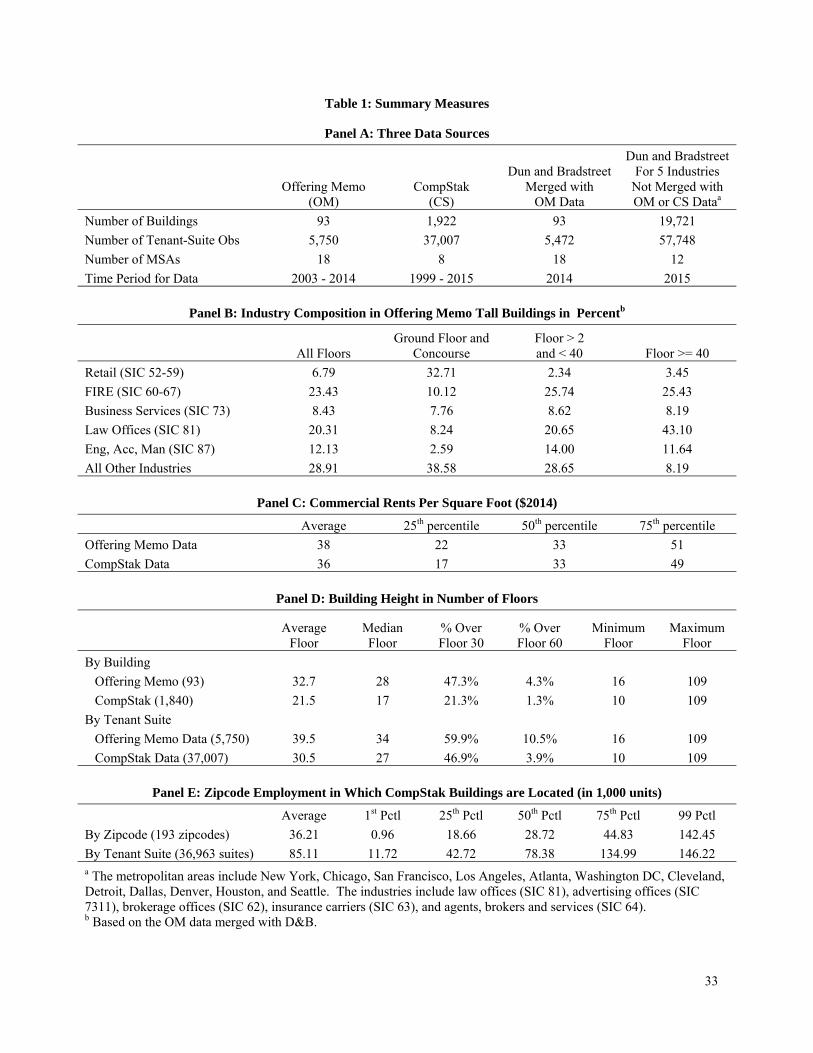
33

Table 1: Summary Measures

Panel A: Three Data Sources

Offering Memo

(OM) CompStak

(CS)

Dun and Bradstreet Merged with

OM Data

Dun and Bradstreet For 5 Industries

Not Merged with OM or CS Dataa

Number of Buildings 93 1,922 93 19,721

Number of Tenant-Suite Obs 5,750 37,007 5,472 57,748

Number of MSAs 18 8 18 12

Time Period for Data 2003 - 2014 1999 - 2015 2014 2015

Panel B: Industry Composition in Offering Memo Tall Buildings in Percentb

All Floors Ground Floor and

Concourse Floor > 2 and < 40 Floor >= 40

Retail (SIC 52-59) 6.79 32.71 2.34 3.45

FIRE (SIC 60-67) 23.43 10.12 25.74 25.43

Business Services (SIC 73) 8.43 7.76 8.62 8.19

Law Offices (SIC 81) 20.31 8.24 20.65 43.10

Eng, Acc, Man (SIC 87) 12.13 2.59 14.00 11.64

All Other Industries 28.91 38.58 28.65 8.19

Panel C: Commercial Rents Per Square Foot ($2014)

Average 25th percentile 50th percentile 75th percentile

Offering Memo Data 38 22 33 51

CompStak Data 36 17 33 49

Panel D: Building Height in Number of Floors

Average

Floor Median Floor

% Over Floor 30

% Over Floor 60

Minimum Floor

Maximum Floor

By Building

Offering Memo (93) 32.7 28 47.3% 4.3% 16 109

CompStak (1,840) 21.5 17 21.3% 1.3% 10 109

By Tenant Suite

Offering Memo Data (5,750) 39.5 34 59.9% 10.5% 16 109

CompStak Data (37,007) 30.5 27 46.9% 3.9% 10 109

Panel E: Zipcode Employment in Which CompStak Buildings are Located (in 1,000 units)

Average 1st Pctl 25th Pctl 50th Pctl 75th Pctl 99 Pctl

By Zipcode (193 zipcodes) 36.21 0.96 18.66 28.72 44.83 142.45

By Tenant Suite (36,963 suites) 85.11 11.72 42.72 78.38 134.99 146.22 a The metropolitan areas include New York, Chicago, San Francisco, Los Angeles, Atlanta, Washington DC, Cleveland, Detroit, Dallas, Denver, Houston, and Seattle. The industries include law offices (SIC 81), advertising offices (SIC 7311), brokerage offices (SIC 62), insurance carriers (SIC 63), and agents, brokers and services (SIC 64). b Based on the OM data merged with D&B.

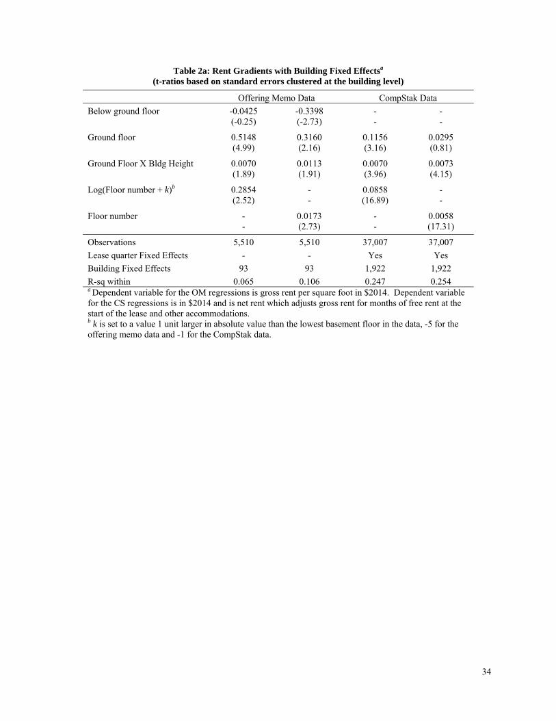
34

Table 2a: Rent Gradients with Building Fixed Effectsa

(t-ratios based on standard errors clustered at the building level)

Offering Memo Data CompStak Data

Below ground floor -0.0425 -0.3398 - - (-0.25) (-2.73) - -

Ground floor 0.5148 0.3160 0.1156 0.0295 (4.99) (2.16) (3.16) (0.81)

Ground Floor X Bldg Height 0.0070 0.0113 0.0070 0.0073 (1.89) (1.91) (3.96) (4.15)

Log(Floor number + k)b 0.2854 - 0.0858 - (2.52) - (16.89) -

Floor number - 0.0173 - 0.0058 - (2.73) - (17.31)

Observations 5,510 5,510 37,007 37,007

Lease quarter Fixed Effects - - Yes Yes

Building Fixed Effects 93 93 1,922 1,922

R-sq within 0.065 0.106 0.247 0.254 a Dependent variable for the OM regressions is gross rent per square foot in $2014. Dependent variable for the CS regressions is in $2014 and is net rent which adjusts gross rent for months of free rent at the start of the lease and other accommodations. b k is set to a value 1 unit larger in absolute value than the lowest basement floor in the data, -5 for the offering memo data and -1 for the CompStak data.

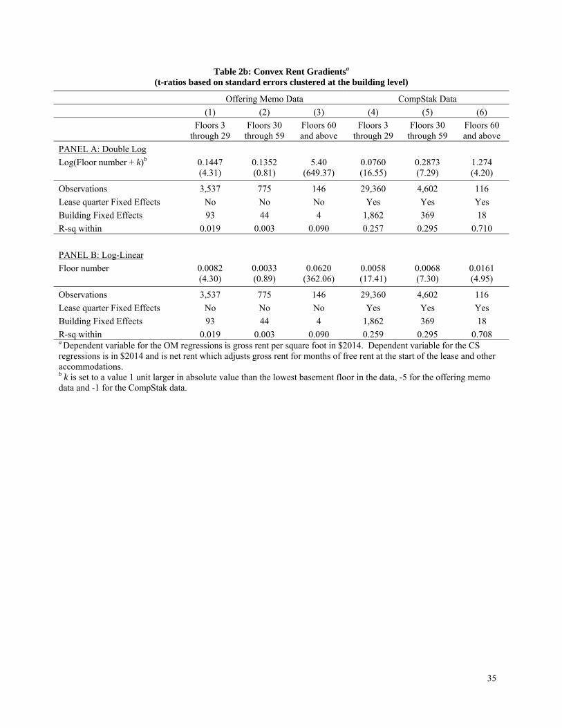
35

Table 2b: Convex Rent Gradientsa

(t-ratios based on standard errors clustered at the building level)

Offering Memo Data CompStak Data

(1) (2) (3) (4) (5) (6)

Floors 3

through 29 Floors 30

through 59 Floors 60 and above

Floors 3 through 29

Floors 30 through 59

Floors 60 and above

PANEL A: Double Log

Log(Floor number + k)b 0.1447 0.1352 5.40 0.0760 0.2873 1.274 (4.31) (0.81) (649.37) (16.55) (7.29) (4.20)

Observations 3,537 775 146 29,360 4,602 116

Lease quarter Fixed Effects No No No Yes Yes Yes

Building Fixed Effects 93 44 4 1,862 369 18

R-sq within 0.019 0.003 0.090 0.257 0.295 0.710

PANEL B: Log-Linear

Floor number 0.0082 0.0033 0.0620 0.0058 0.0068 0.0161 (4.30) (0.89) (362.06) (17.41) (7.30) (4.95)

Observations 3,537 775 146 29,360 4,602 116

Lease quarter Fixed Effects No No No Yes Yes Yes

Building Fixed Effects 93 44 4 1,862 369 18

R-sq within 0.019 0.003 0.090 0.259 0.295 0.708 a Dependent variable for the OM regressions is gross rent per square foot in $2014. Dependent variable for the CS regressions is in $2014 and is net rent which adjusts gross rent for months of free rent at the start of the lease and other accommodations. b k is set to a value 1 unit larger in absolute value than the lowest basement floor in the data, -5 for the offering memo data and -1 for the CompStak data.

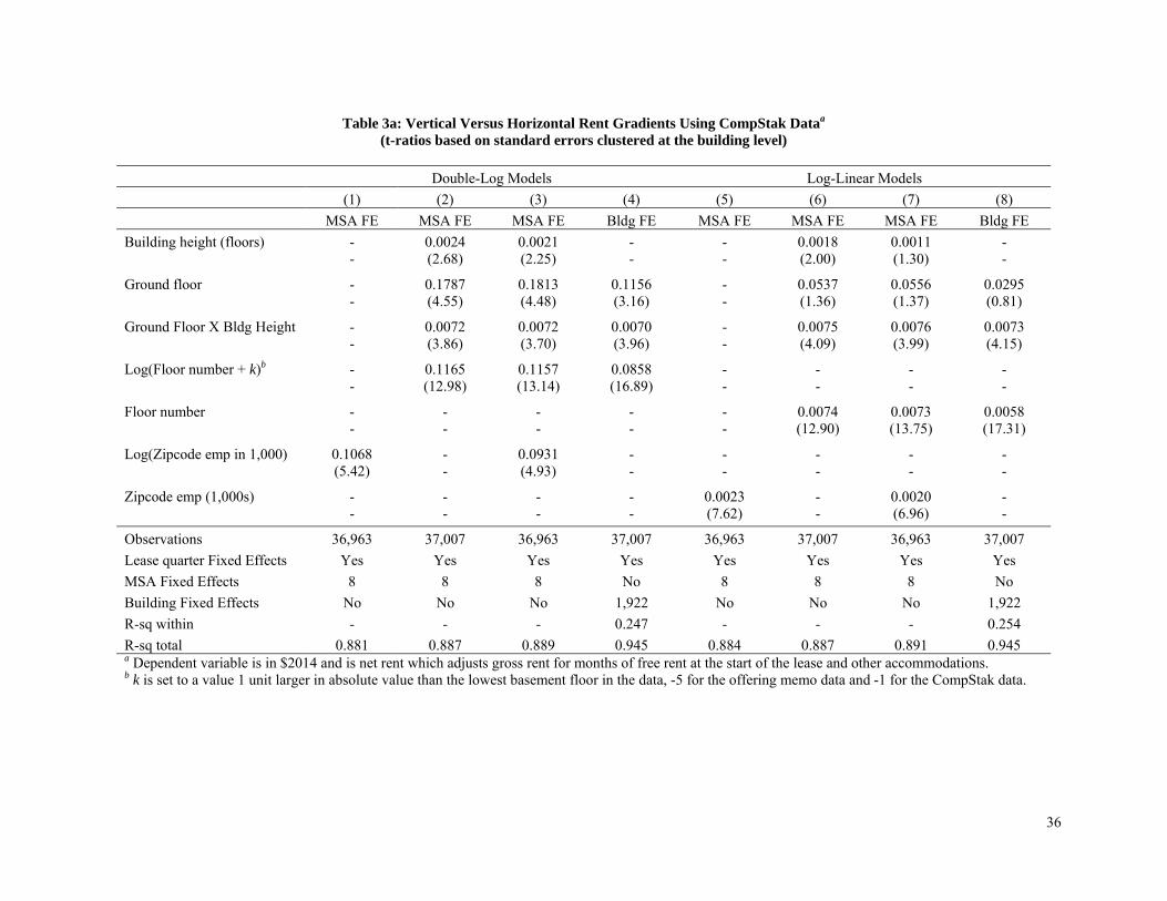
36

Table 3a: Vertical Versus Horizontal Rent Gradients Using CompStak Dataa

(t-ratios based on standard errors clustered at the building level)

Double-Log Models Log-Linear Models

(1) (2) (3) (4) (5) (6) (7) (8)

MSA FE MSA FE MSA FE Bldg FE MSA FE MSA FE MSA FE Bldg FE

Building height (floors) - 0.0024 0.0021 - - 0.0018 0.0011 - - (2.68) (2.25) - - (2.00) (1.30) -

Ground floor - 0.1787 0.1813 0.1156 - 0.0537 0.0556 0.0295 - (4.55) (4.48) (3.16) - (1.36) (1.37) (0.81)

Ground Floor X Bldg Height - 0.0072 0.0072 0.0070 - 0.0075 0.0076 0.0073 - (3.86) (3.70) (3.96) - (4.09) (3.99) (4.15)

Log(Floor number + k)b - 0.1165 0.1157 0.0858 - - - - - (12.98) (13.14) (16.89) - - - -

Floor number - - - - - 0.0074 0.0073 0.0058 - - - - - (12.90) (13.75) (17.31)

Log(Zipcode emp in 1,000) 0.1068 - 0.0931 - - - - - (5.42) - (4.93) - - - - -

Zipcode emp (1,000s) - - - - 0.0023 - 0.0020 - - - - - (7.62) - (6.96) -

Observations 36,963 37,007 36,963 37,007 36,963 37,007 36,963 37,007

Lease quarter Fixed Effects Yes Yes Yes Yes Yes Yes Yes Yes

MSA Fixed Effects 8 8 8 No 8 8 8 No

Building Fixed Effects No No No 1,922 No No No 1,922

R-sq within - - - 0.247 - - - 0.254

R-sq total 0.881 0.887 0.889 0.945 0.884 0.887 0.891 0.945 a Dependent variable is in $2014 and is net rent which adjusts gross rent for months of free rent at the start of the lease and other accommodations. b k is set to a value 1 unit larger in absolute value than the lowest basement floor in the data, -5 for the offering memo data and -1 for the CompStak data.

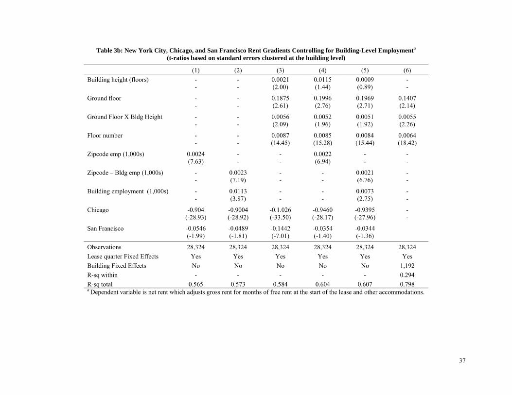
37

Table 3b: New York City, Chicago, and San Francisco Rent Gradients Controlling for Building-Level Employmenta

(t-ratios based on standard errors clustered at the building level)

(1) (2) (3) (4) (5) (6)

Building height (floors) - - 0.0021 0.0115 0.0009 - - - (2.00) (1.44) (0.89) -

Ground floor - - 0.1875 0.1996 0.1969 0.1407 - - (2.61) (2.76) (2.71) (2.14)

Ground Floor X Bldg Height - - 0.0056 0.0052 0.0051 0.0055 - - (2.09) (1.96) (1.92) (2.26)

Floor number - - 0.0087 0.0085 0.0084 0.0064 - - (14.45) (15.28) (15.44) (18.42)

Zipcode emp (1,000s) 0.0024 - - 0.0022 - - (7.63) - - (6.94) - -

Zipcode – Bldg emp (1,000s) - 0.0023 - - 0.0021 - - (7.19) - - (6.76) -

Building employment (1,000s) - 0.0113 - - 0.0073 - - (3.87) - - (2.75) -

Chicago -0.904 -0.9004 -0.1.026 -0.9460 -0.9395 - (-28.93) (-28.92) (-33.50) (-28.17) (-27.96) -

San Francisco -0.0546 -0.0489 -0.1442 -0.0354 -0.0344 (-1.99) (-1.81) (-7.01) (-1.40) (-1.36)

Observations 28,324 28,324 28,324 28,324 28,324 28,324

Lease quarter Fixed Effects Yes Yes Yes Yes Yes Yes

Building Fixed Effects No No No No No 1,192

R-sq within - - - - - 0.294

R-sq total 0.565 0.573 0.584 0.604 0.607 0.798 a Dependent variable is net rent which adjusts gross rent for months of free rent at the start of the lease and other accommodations.

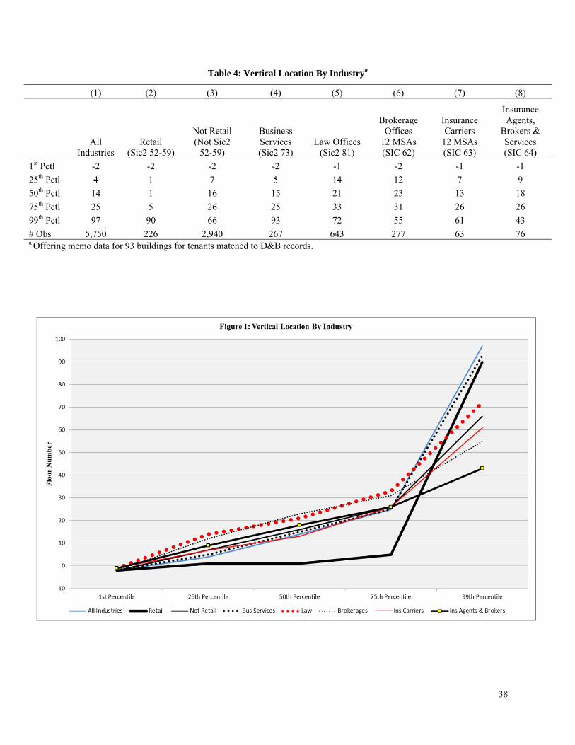
38

Table 4: Vertical Location By Industrya

(1) (2) (3) (4) (5) (6) (7) (8)

All

Industries Retail

(Sic2 52-59)

Not Retail (Not Sic2

52-59)

Business Services (Sic2 73)

Law Offices (Sic2 81)

Brokerage Offices

12 MSAs (SIC 62)

Insurance Carriers

12 MSAs (SIC 63)

Insurance Agents,

Brokers & Services (SIC 64)

1st Pctl -2 -2 -2 -2 -1 -2 -1 -1

25th Pctl 4 1 7 5 14 12 7 9

50th Pctl 14 1 16 15 21 23 13 18

75th Pctl 25 5 26 25 33 31 26 26

99th Pctl 97 90 66 93 72 55 61 43

# Obs 5,750 226 2,940 267 643 277 63 76 a Offering memo data for 93 buildings for tenants matched to D&B records.

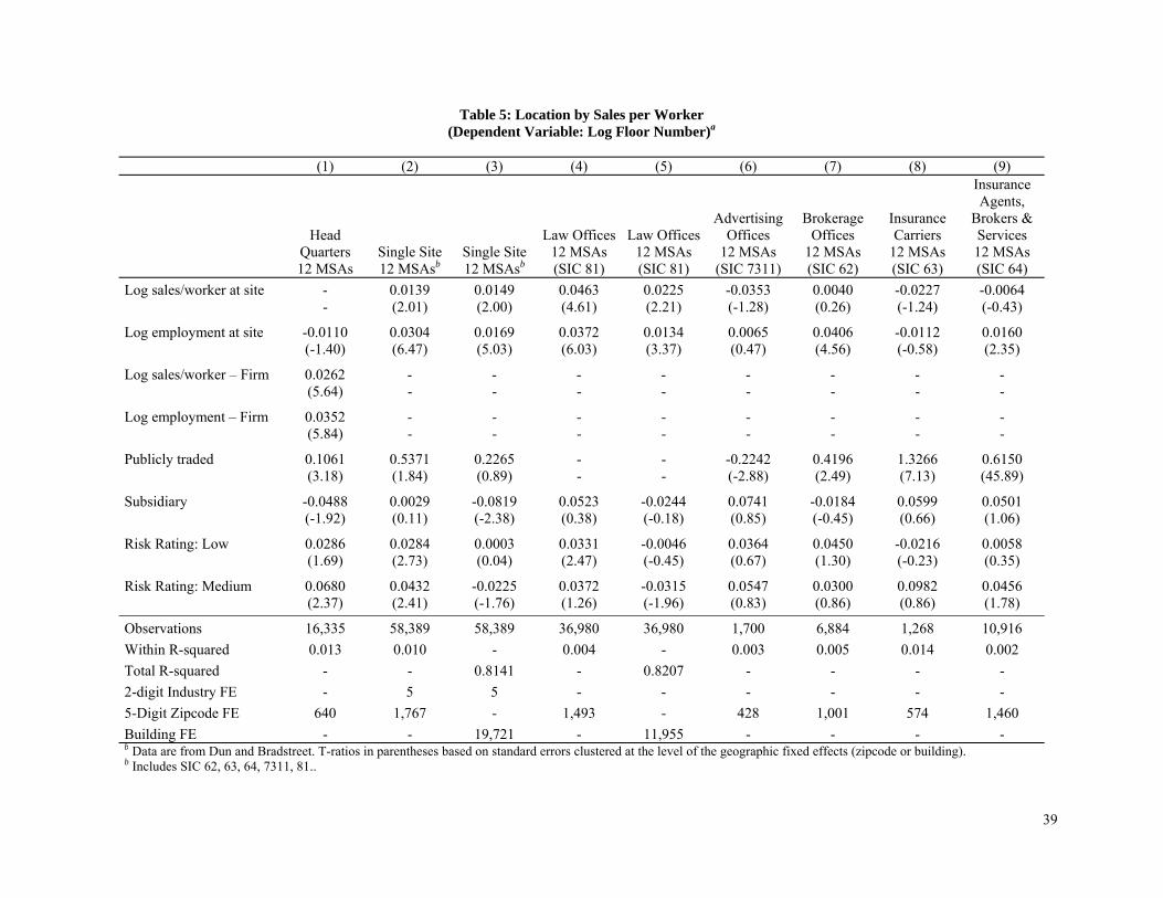
39

Table 5: Location by Sales per Worker (Dependent Variable: Log Floor Number)a

(1) (2) (3) (4) (5) (6) (7) (8) (9)

Head Quarters 12 MSAs

Single Site 12 MSAsb

Single Site 12 MSAsb

Law Offices 12 MSAs (SIC 81)

Law Offices 12 MSAs (SIC 81)

Advertising Offices

12 MSAs (SIC 7311)

Brokerage Offices

12 MSAs (SIC 62)

Insurance Carriers

12 MSAs (SIC 63)

Insurance Agents,

Brokers & Services 12 MSAs (SIC 64)

Log sales/worker at site - 0.0139 0.0149 0.0463 0.0225 -0.0353 0.0040 -0.0227 -0.0064 - (2.01) (2.00) (4.61) (2.21) (-1.28) (0.26) (-1.24) (-0.43)

Log employment at site -0.0110 0.0304 0.0169 0.0372 0.0134 0.0065 0.0406 -0.0112 0.0160 (-1.40) (6.47) (5.03) (6.03) (3.37) (0.47) (4.56) (-0.58) (2.35)

Log sales/worker – Firm 0.0262 - - - - - - - - (5.64) - - - - - - - -

Log employment – Firm 0.0352 - - - - - - - - (5.84) - - - - - - - -

Publicly traded 0.1061 0.5371 0.2265 - - -0.2242 0.4196 1.3266 0.6150 (3.18) (1.84) (0.89) - - (-2.88) (2.49) (7.13) (45.89)

Subsidiary -0.0488 0.0029 -0.0819 0.0523 -0.0244 0.0741 -0.0184 0.0599 0.0501 (-1.92) (0.11) (-2.38) (0.38) (-0.18) (0.85) (-0.45) (0.66) (1.06)

Risk Rating: Low 0.0286 0.0284 0.0003 0.0331 -0.0046 0.0364 0.0450 -0.0216 0.0058 (1.69) (2.73) (0.04) (2.47) (-0.45) (0.67) (1.30) (-0.23) (0.35)

Risk Rating: Medium 0.0680 0.0432 -0.0225 0.0372 -0.0315 0.0547 0.0300 0.0982 0.0456 (2.37) (2.41) (-1.76) (1.26) (-1.96) (0.83) (0.86) (0.86) (1.78)

Observations 16,335 58,389 58,389 36,980 36,980 1,700 6,884 1,268 10,916

Within R-squared 0.013 0.010 - 0.004 - 0.003 0.005 0.014 0.002

Total R-squared - - 0.8141 - 0.8207 - - - -

2-digit Industry FE - 5 5 - - - - - -

5-Digit Zipcode FE 640 1,767 - 1,493 - 428 1,001 574 1,460

Building FE - - 19,721 - 11,955 - - - - b Data are from Dun and Bradstreet. T-ratios in parentheses based on standard errors clustered at the level of the geographic fixed effects (zipcode or building). b Includes SIC 62, 63, 64, 7311, 81..

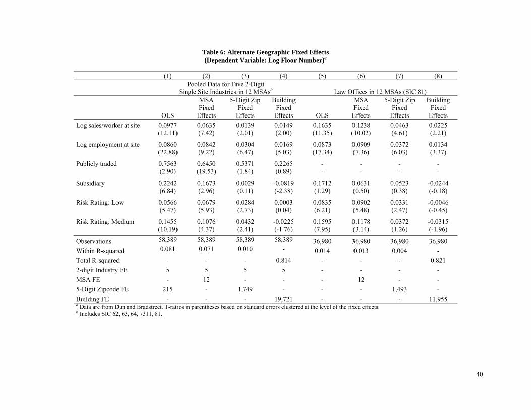
40

Table 6: Alternate Geographic Fixed Effects (Dependent Variable: Log Floor Number)a

(1) (2) (3) (4) (5) (6) (7) (8)

Pooled Data for Five 2-Digit

Single Site Industries in 12 MSAsb Law Offices in 12 MSAs (SIC 81)

OLS

MSA Fixed

Effects

5-Digit Zip Fixed

Effects

Building Fixed

Effects OLS

MSA Fixed

Effects

5-Digit Zip Fixed

Effects

Building Fixed

Effects

Log sales/worker at site 0.0977 0.0635 0.0139 0.0149 0.1635 0.1238 0.0463 0.0225 (12.11) (7.42) (2.01) (2.00) (11.35) (10.02) (4.61) (2.21)

Log employment at site 0.0860 0.0842 0.0304 0.0169 0.0873 0.0909 0.0372 0.0134 (22.88) (9.22) (6.47) (5.03) (17.34) (7.36) (6.03) (3.37)

Publicly traded 0.7563 0.6450 0.5371 0.2265 - - - - (2.90) (19.53) (1.84) (0.89) - - - -

Subsidiary 0.2242 0.1673 0.0029 -0.0819 0.1712 0.0631 0.0523 -0.0244 (6.84) (2.96) (0.11) (-2.38) (1.29) (0.50) (0.38) (-0.18)

Risk Rating: Low 0.0566 0.0679 0.0284 0.0003 0.0835 0.0902 0.0331 -0.0046 (5.47) (5.93) (2.73) (0.04) (6.21) (5.48) (2.47) (-0.45)

Risk Rating: Medium 0.1455 0.1076 0.0432 -0.0225 0.1595 0.1178 0.0372 -0.0315 (10.19) (4.37) (2.41) (-1.76) (7.95) (3.14) (1.26) (-1.96)

Observations 58,389 58,389 58,389 58,389 36,980 36,980 36,980 36,980

Within R-squared 0.081 0.071 0.010 - 0.014 0.013 0.004 -

Total R-squared - - - 0.814 - - - 0.821

2-digit Industry FE 5 5 5 5 - - - -

MSA FE - 12 - - - 12 - -

5-Digit Zipcode FE 215 - 1,749 - - - 1,493 -

Building FE - - - 19,721 - - - 11,955 a Data are from Dun and Bradstreet. T-ratios in parentheses based on standard errors clustered at the level of the fixed effects. b Includes SIC 62, 63, 64, 7311, 81.

41

Appendix A: Offering Memo Example

JP Morgan Chase Commercial Mortgage Securities Trust 2006-LDP723

One Prudential Plaza Stacking Plan

Flr Tenant SqFt Lease Ends

Tenant SqFt Lease Ends

41 Plaza Club 7,798 06/06 40M AM/FM Ohio, Inc 100 09/06 40 Vacant 1,860 Multi-Tenant 8,254 39 Baker & McKenzie LLP 22,503 11/12 38 Schuyler, Roche & Zwirner 24,082 04/15 37 Baker & McKenzie LLP 24,017 11/12 36 Baker & McKenzie LLP 24,068 11/12 35 Baker & McKenzie LLP 24,148 11/12 34 Vacant 14,274 Baker & McKenzie LLP 8,917 12/08 33 Baker & McKenzie LLP 23,026 11/12 32 Baker & McKenzie LLP 22,411 11/12 31 Baker & McKenzie LLP 22,990 11/12 30 Baker & McKenzie LLP 21,191 11/12 29 McGraw-Hill Inc 22,647 11/16 28 Baker & McKenzie LLP 9,747 11/12 BDO Seidman, LLP 12186 09/11 27 Bonneville International 21,913 05/18 26 Multi-Tenant 21,742 25 Baker & McKenzie LLP 22,862 11/12 24 Peoples Gas Light & Coke 21,803 05/14 23 Peoples Gas Light & Coke 21,803 05/14 22 Peoples Gas Light & Coke 21,803 05/14 21 Peoples Gas Light & Coke 22,862 05/14 20 Peoples Gas Light & Coke 23,264 05/14 19 Peoples Gas Light & Coke 21,321 05/14 18 Peoples Gas Light & Coke 19,917 05/14 17 Peoples Gas Light & Coke 23,203 05/14 16 Peoples Gas Light & Coke 23,126 05/14

15 Atty Regis & Disciplinary Commission 23,125 05/15

14 Vacant 1,208 McGraw-Hill, Inc 23,199 11/16 13 Vacant 22,398 BDO Seidman, LLP 383 09/06 12 Vacant 1,991 Multi-Tenant 21,375 11 Multi-Tenant 22,397 10 Vacant 1,009 Multi-Tenant 47,600 9 McGraw-Hill, Inc 49,998 11/16 8 Vacant 48,818 7 Vacant 19,655 Kirkland & Ellis LLP 28,154 12/11 6 Kirkland & Ellis LLP 52,224 21/11 5 BCE Nexxia Corp 49,144 08/15 4 McGraw-Hill, Inc 49,252 11/16 3 Peoples Gas Light & Coke 48,784 05/14

23http://www.secinfo.com/dsvrn.v4Mq.htm

42

Appendix A (continued) JP Morgan Chase Commercial Mortgage Securities Trust 2006-LDP724

One Prudential Plaza Stacking Plan

Flr Tenant SqFt Lease

Ends Tenant SqFt Lease

Ends 2 Vacant 5 Multi-Tenant 36,763 1 Vacant 19,239 Multi-Tenant 22,151 Entr Vacant 2,011 Multi-Tenant 34,148 B2 Peoples Gas Light & Coke 267 05/14 B1 Vacant 8,005 Multi-Tenant 9,662

Two Prudential Plaza Stacking Plan

Flr Tenant SqFt Lease

Ends Tenant SqFt Lease

Ends 58 Taipei Econ/ Cultural Ofc 12,994 06/11 57 Taipei Econ/ Cultural Ofc 10,267 06/11 Advisory Research Inc. 2,943 05/14 58 Taipei Econ/ Cultural Ofc 12,994 06/11 56 Prudential Insurance Co. 13,717 07/08 55 Multi-Tenant 14,000 54 Prudential Insurance Co. 14,082 07/08 53 Multi-Tenant 12,822 Vacant 1,325 52 Vacant 14,038 51 Centraxcorp 14,932 03/16 50 Leydig, Voit & Mayer Ltd 15,164 08/10 49 Leydig, Voit & Mayer Ltd 16,000 08/10 48 Leydig, Voit & Mayer Ltd 16,000 08/10 47 Leydig, Voit & Mayer Ltd 9,704 08/10 Prudential Insurance Co. 7,540 07/08 46 Prophet Brand Strategy 17,950 03/12 45 Multi-Tenant 17,950 44 International Food Svc 9,747 11/13 Vacant 8,203 43 Black Entertainment TV 9,647 08/07 BDO Seidman, LLP 8,303 42 Aleri, Inc 18,726 10/07 41 Aleri, Inc 19,000 10/07 40 Aleri, Inc 19,565 10/07 39 Mechanical Room 38 Bowman, Barrett & Assoc 162 11/06 Mechanical Room 1,313 38 37 Leboeuf, Lamb, Greene &

Macrae 20,184 09/10

36 Norgren, Inc 6,560 09/12 Vacant 13,555 35 Vacant 20,174 34 Vacant 20,743 33 Vacant 20,219 32 Multi-Tenant 18,223 Vacant 2,007

Appendix B (continued) JP Morgan Chase Commercial Mortgage Securities Trust 2006-LDP725

24http://www.secinfo.com/dsvrn.v4Mq.htm 25http://www.secinfo.com/dsvrn.v4Mq.htm

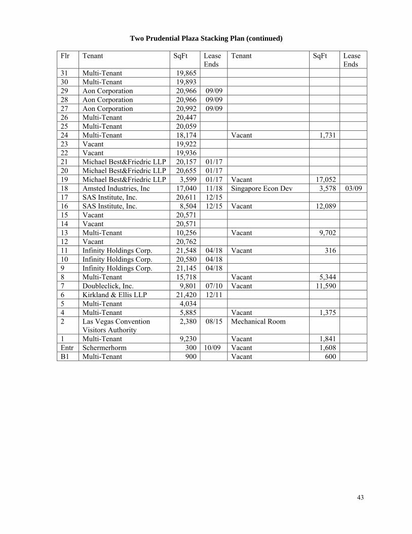
43

Two Prudential Plaza Stacking Plan (continued)

Flr Tenant SqFt Lease Ends

Tenant SqFt Lease Ends

31 Multi-Tenant 19,865 30 Multi-Tenant 19,893 29 Aon Corporation 20,966 09/09 28 Aon Corporation 20,966 09/09 27 Aon Corporation 20,992 09/09 26 Multi-Tenant 20,447 25 Multi-Tenant 20,059 24 Multi-Tenant 18,174 Vacant 1,731 23 Vacant 19,922 22 Vacant 19,936 21 Michael Best&Friedric LLP 20,157 01/17 20 Michael Best&Friedric LLP 20,655 01/17 19 Michael Best&Friedric LLP 3,599 01/17 Vacant 17,052 18 Amsted Industries, Inc 17,040 11/18 Singapore Econ Dev 3,578 03/09 17 SAS Institute, Inc. 20,611 12/15 16 SAS Institute, Inc. 8,504 12/15 Vacant 12,089 15 Vacant 20,571 14 Vacant 20,571 13 Multi-Tenant 10,256 Vacant 9,702 12 Vacant 20,762 11 Infinity Holdings Corp. 21,548 04/18 Vacant 316 10 Infinity Holdings Corp. 20,580 04/18 9 Infinity Holdings Corp. 21,145 04/18 8 Multi-Tenant 15,718 Vacant 5,344 7 Doubleclick, Inc. 9,801 07/10 Vacant 11,590 6 Kirkland & Ellis LLP 21,420 12/11 5 Multi-Tenant 4,034 4 Multi-Tenant 5,885 Vacant 1,375 2 Las Vegas Convention

Visitors Authority 2,380 08/15 Mechanical Room

1 Multi-Tenant 9,230 Vacant 1,841 Entr Schermerhorm 300 10/09 Vacant 1,608 B1 Multi-Tenant 900 Vacant 600

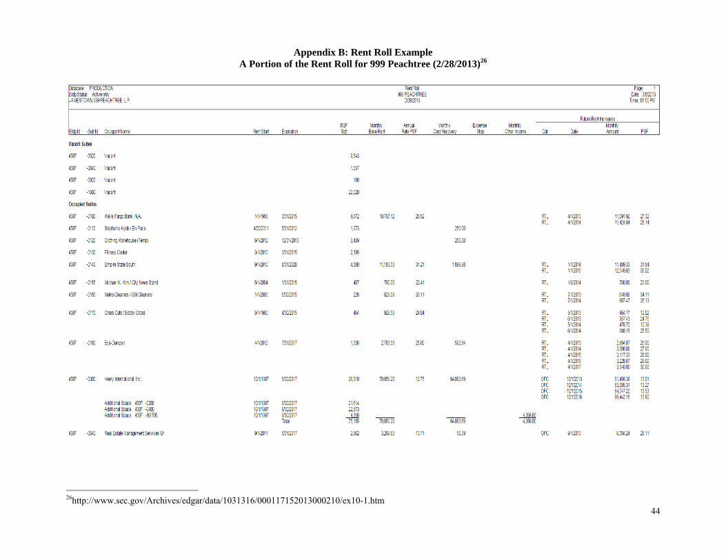
44

Appendix B: Rent Roll Example A Portion of the Rent Roll for 999 Peachtree (2/28/2013)26

26http://www.sec.gov/Archives/edgar/data/1031316/000117152013000210/ex10-1.htm

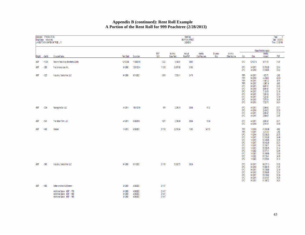
45

Appendix B (continued): Rent Roll Example A Portion of the Rent Roll for 999 Peachtree (2/28/2013)