arX

iv:h

ep-t

h/93

1210

4v1

13

Dec

199

3

IASSNS-HEP-93/41

December, 1993

THE VERLINDE ALGEBRA AND THE

COHOMOLOGY OF THE GRASSMANNIAN

Edward Witten⋆

School of Natural Sciences

Institute for Advanced Study

Olden Lane

Princeton, NJ 08540

ABSTRACT

The article is devoted to a quantum field theory explanation of the relationship

between the Verlinde algebra of the group U(k) at level N − k and the “quantum”

cohomology of the Grassmannian of complex k planes in N space. In §2, I explain

the relation between the Verlinde algebra and the gauged WZW model of G/G; in

§3, I describe the quantum cohomology and its origin in a quantum field theory;

and in §4, I present a path integral argument for mapping between them.

⋆ Research supported in part by NSF Grant PHY92-45317.

1. Introduction

My main goal in these lecture notes will be to elucidate a formula of Doron

Gepner [1], which relates two mathematical objects, one rather old and one rather

new. Along the way we will consider a few other matters as well.

The old structure is the cohomology ring of the Grassmannian G(k,N) of

complex k planes in N space – except that one considers the quantum cohomology

(or Floer instanton homology) rather than the classical cohomology. The new

structure is the Verlinde algebra, which computes the Hilbert polynomial of the

moduli space of vector bundles on a curve. Gepner’s formula, as we will consider

it here,†

says that the quantum cohomology ring of G(k,N) coincides with the

Verlinde algebra of the group U(k) essentially at level N − k.‡

Gepner discovered his formula by computing the left and right hand side and

observing that they were equal. We will seek a more conceptual explanation, by

representing the quantum cohomology ring of the Grassmannian in a quantum field

theory and reducing that quantum field theory at low energies to another quantum

field theory which is known to compute the Verlinde algebra.

The Verlinde formula appears in several quantum field theories. Of these, the

one that is relevant here is the gauged WZW model, ofG/G. The shortest and most

complete explanation of its relation to the Verlinde formula is due to Gerasimov

[4], and I will explain his argument in §2. Part of the charm of the G/G model is

that it can be abelianized, that is, reduced to a theory in which the gauge group is

the maximal torus of G, extended by the Weyl group [5]. The argument is simple

in concept and will be summarized in §2.6.

In §3, I explain at a qualitative level how the quantum cohomology of the Grass-

† Gepner actually discusses the classical cohomology of the Grassmannian and identifies itwith a close cousin of the Verlinde algebra. The refinement of Gepner’s formula that wewill consider was conjectured by Vafa [2] and Intriligator [3].

‡ Actually if one decomposes the Lie algebra of U(k) as su(k) × u(1), then the level is (N −k,N), that is level N − k for the su(k) factor and level N for the u(1) factor. The sourceof this subtlety will become clear in §4.6.

2

mannian is represented in a quantum field theory, and some general techniques for

studying this field theory and reducing it to a problem in gauge theory. In §4, I

describe the arguments in more technical detail. The analysis actually should be

adaptable to other manifolds that can be realized as symplectic quotients of linear

spaces, such as flag manifolds and toric varieties. (The quantum cohomology of a

toric variety has been studied by Batyrev [6]; that of a general flag manifold has

apparently not yet been studied.)

This paper, despite its length, is based on an idea that can be described very

simply. The two dimensional supersymmetric sigma model with target G(k,N)

can be described as a U(k) gauge theory (in N = 2 superspace) with N multiplets

of chiral superfields in the fundamental representation of U(k). It was studied from

this point of view in the case of k = 1 (that is CPN−1) many years ago [7,8], and

the generalization to arbitrary k is also familiar [9,10]. At low energy, a suitable

U(k) gauge theory with the matter content just stated reduces to the supersym-

metric sigma model of the Grassmannian. On the other hand, integrating out the

N matter multiplets, one gets an effective action for the U(k) gauge multiplet.

Because of a sort of mixing between scalars and vectors, this low energy effective

action has no massless particles; this is how the presence of a mass gap has been

shown in the past. The novelty in the present paper is simply the observation

that the low energy effective action is in fact a gauged WZW model of U(k)/U(k).

Under this low energy reduction, the topological correlation functions of the sigma

model – which compute the quantum cohomology of G(k,N) – are mapped into

correlation functions of the U(k)/U(k) model that can be computed (as we recall in

§2) in terms of the Verlinde algebra. This gives the map between the two theories.

The quantum cohomology of the Grassmannian has also been studied – using,

more or less, a classical version of the same setup we will follow – by Bertram,

Daskapoulos, and Wentworth [11]. And there is a forthcoming mathematical ap-

proach to Gepner’s formula in work of Braam and Agnihorti. The cohomology of

the Grassmannian is closely related to the chiral ring of a certain N = 2 supercon-

formal field theory [12] (somewhat misleadingly called a U(N)/U(k) × U(N − k)

3

coset model); this model probably should be included in the story, but that will

not be done here. Some of the phenomena we will study have analogs for real and

symplectic Grassmannians, as in [13] and the second paper cited in [1]; it would

be interesting to try to extend the analysis for those cases.

§2 and §3 can be read independently of one another. §4 requires more famil-

iarity with methods of physics than either §2 or §3. Physicists may want to start

with §4.

2. The Verlinde Formula And The G/G Model

First of all, the Verlinde algebra counts theta functions, such as the classical

theta functions of Jacobi and their generalizations. In modern language, the clas-

sical theta functions can be described as follows. Let T be a complex torus of

dimensions g, L a line bundle defining a principal polarization, and s a positive

integer. Then the space of level s theta functions is H0(T ,L⊗s). The dimension

of this space can be readily determined from the Riemann-Roch theorem.

For example, T might be the Jacobian J of a complex Riemann surface Σ,

that is, the moduli space of holomorphic line bundles over Σ of some given degree.

This example suggests the generalization to the “non-abelian theta functions” of A.

Weil. Here one replaces the Jacobian of Σ by the moduli space R of rank k (stable)

holomorphic vector bundles over Σ; now a “non-abelian theta function” at level s

is an element of H0(R,L⊗s). Though the Riemann-Roch theorem gives a formula

for the dimension of this space, this formula is difficult to use in the non-abelian

case as it involves invariants of R that are not easy to determine directly.

The Verlinde algebra gives on the other hand a practical formula for the di-

mension of H0(R,L⊗s); the formula was described very explicitly by Raoul Bott

in [14]. Roughly speaking, the origin of the Verlinde formula in differential geom-

etry is as follows. Via Hodge theory, R is endowed with a natural Kahler metric.

As the dimension of the space of non-abelian theta functions is independent of

4

the complex structure of Σ, one can choose the complex structure to simplify the

problem. It is convenient to take Σ to be a nearly degenerate surface consisting

of three-holed spheres joined by long tubes. Using the behavior of the differential

geometry of R in this limit, one can write H0(R,L⊗s) as a sum of tensor products

of similar spaces for a three-holed sphere with some branching around the holes.

The Verlinde algebra encodes the details of this.

The Verlinde algebra arises in several quantum field theories:

(1) It originally arose [15] in the WZW model, a conformal field theory (whose

Lagrangian we will recall later) that governs maps from a Riemann surface Σ to

a compact Lie group G. Mathematically, this model is related to representations

of affine Lie algebras, the unitary action of the modular group SL(2,Z) on their

characters, etc.

(2) The Verlinde formula is an important ingredient in understanding Chern-

Simons gauge theory on a three-manifold. Thus it is relevant to the knot and

three-manifold invariants constructed from quantum field theory.

(3) The Verlinde formula also enters in the gauged WZW model, governing a

pair (g, A), where A is a connection on a principal G bundle P over a Riemann

surface, and g is a section of P ×GG (where G acts on itself via the adjoint action).

Of these it is the third – which was discovered most recently – that will enter

our story. The present section is therefore mainly devoted to an explanation –

following Gerasimov [4], who reinterpreted earlier formulas [16,17] – of the gauged

WZW model and its relation to nonabelian theta functions.

2.1. Gauge Theory And The Prequantum Line Bundle In Two Di-

mensions

Let G be a compact Lie group, Σ a closed oriented two-manifold without

boundary, and P a principal G bundle over Σ. To achieve some minor simplifica-

tions in the exposition, I will suppose G simple, connected, and simply connected.

5

(Notation aside, the only novelty required to treat a general compact Lie group is

that more care is required in defining the functional Γ(g, A) that appears below;

see [18, §4].) One consequence of the assumption about G is that P is trivial.

Let A be the space of connections on P . A has a natural symplectic structure

ω that can be defined with no choice of metric or complex structure on Σ. (This

and some other facts that I summarize presently are originally due to Atiyah and

Bott [20].) The symplectic structure can be defined by the formula

ω(a1, a2) =1

2π

∫

Σ

Tr a1 ∧ a2, (2.1)

where a1 and a2 are adjoint-valued one-forms representing tangent vectors to A.

Here Tr is an invariant quadratic form on the Lie algebra of G, defined for G =

SU(k) to be the trace in the k dimensional representation; in general one can take

Tr to be the smallest positive multiple of the trace in the adjoint representation

such that the differential form Θ introduced below has periods that are multiples

of 2π.

A prequantum line bundle L over A is a unitary line bundle with a connection

of curvature −iω. L exists and is unique up to isomorphism since A is an affine

space. We can take L to be the trivial bundle with a connection defined by the

following formula:

D

DAi=

δ

δAi+

i

4πǫijAj . (2.2)

(ǫij is the Levi-Civita antisymmetric tensor; when local complex coordinates are

introduced, we will take ǫzz = −ǫzz = i.) The kth power L⊗k is therefore the

trivial bundle endowed with the connection

D

DAi=

δ

δAi+ik

4πǫijAj . (2.3)

Let G be the group of gauge transformations. If P is trivialized, a gauge

6

transformation is a map g : Σ → G, and acts on the connection A by

A→ Ag = gAg−1 − dg · g−1. (2.4)

More invariantly, g is a section of P ×G G, where G acts on itself in the adjoint

representation, and the action of g on A should be written as

dA → gdAg−1, (2.5)

with dA the gauge-covariant extension of the exterior derivative. At the Lie algebra

level this is

A→ A− dAα, (2.6)

where α is a section of P ×G g, with g being the Lie algebra of G, on which G acts

by the adjoint action.

The action of the gauge group on the space A of connections lifts to an action

on the prequantum line bundle. At the Lie algebra level, the lift is generated by

the operators

DiD

DAi− ik

4πǫijFij , (2.7)

with F = dA + A ∧ A the curvature form. (2.7) means very concretely that the

infinitesimal gauge transformation (2.6) is represented on sections of L by the

operator∫

Σ

Trα

(Di

D

DAi− ik

4πF

). (2.8)

Even globally, at the group level, the G action on L can be described rather

explicitly [21]. Pick a three manifold B with ∂B = Σ. Given g : Σ → G, extend g

to a map (which I will also call g) from B to G. (The extension exists because of

7

our assumption that π0(G) = π1(G) = 0. See [19,18] for the definition of Γ without

this simplifying assumption.) Define as in [22]

Γ(g) =1

12π

∫

B

Tr g−1dg ∧ g−1dg ∧ g−1dg, (2.9)

which is known as the Wess-Zumino anomaly functional [23]. This is equivalent to

Γ(g) =

∫

B

g∗(Θ), (2.10)

where

Θ =1

12πTr g−1dg ∧ g−1dg ∧ g−1dg (2.11)

is a left- and right-invariant closed three-form on G. The periods of Θ are multiples

of 2π. This ensures that, regarded as a map to R/2πZ, Γ(g) depends only on the

restriction of g to Σ. Note that Γ is defined purely in differential topology; no

metric or complex structure on Σ is required.

It follows rather directly from the definition of Γ that for g, h : Σ → G,

Γ(gh) = Γ(g) + Γ(h) − 1

4π

∫

Σ

Tr g−1dg ∧ dh · h−1. (2.12)

A variant of this equation is called the Polyakov-Wiegmann formula [24].

Now, given a connection A on P , set

W (g, A) = Γ(g) − 1

4π

∫

Σ

TrA ∧ g−1dg. (2.13)

From (2.12), it follows almost immediately that

W (gh, A) = W (g, Ah) +W (h,A). (2.14)

From this we can define an action of the gauge group G on the space of functions

8

of A. In fact, setting

g∗χ(A) = exp(ikW (g, A)) · χ(Ag), (2.15)

we have (gh)∗ = h∗g∗. Differentiating (2.15) with respect to g at g = 1, one sees

that this particular lift induces (2.7) at the Lie algebra level; so (2.15) is the desired

lifting of the action of the gauge group to an action on the prequantum line bundle

L.

2.2. Non-Abelian Theta Functions

So far we have considered Σ simply as a closed, oriented two-manifold without

boundary. If one picks a complex structure on Σ, some additional interesting

constructions can be made [20]. A complex structure on Σ induces a complex

structure on the space A of connections. One simply declares that the (0, 1) part

of A is holomorphic and the (1, 0) part is antiholomorphic. If z, z are local complex

coordinates on Σ, then the connection (2.3) characterizing L⊗k can be written

D

DAz=

δ

δAz− k

4πAz

D

DAz=

δ

δAz+

k

4πAz.

(2.16)

The complex structure on A can be described in very down-to-earth terms by

saying that a holomorphic function on A is a function annihilated by δ/δAz. Cor-

respondingly, a holomorphic section of L⊗k is a section annihilated by D/DAz.

Even more explicitly, a holomorphic section of L⊗k is a function χ(Az, Az) which

can be written

χ(Az , Az) = exp

k

4π

∫

Σ

TrAzAz

· χ(Az), (2.17)

with χ(Az) an ordinary holomorphic function on A.

9

Once a complex structure is picked on Σ, the connection A determines opera-

tors ∂A giving complex structures to vector bundles P×Gr, with r a representation

of G. The action of gauge transformations on A can be described by the action on

the ∂A operators:

∂A → g · ∂A · g−1. (2.18)

Since this formula makes sense for complex g, the G action on A extends to an

action of the complexified gauge group GC (consisting of maps of Σ to the com-

plexification GC of G).

Two ∂A operators define equivalent holomorphic bundles if and only if they

are related as in (2.18). So the quotient A/GC (in case the GC action is not free,

the quotient must be taken in the sense of geometric invariant theory) is the same

as the moduli space R of (stable) holomorphic principal G bundles over Σ.

The formulas used to describe the lift of the G action to L make sense when g

is complex, so we get a lift of the GC action to L. One defines a line bundle over

R – which we will also call L – whose sections over an open set U ⊂ R are the

same as the GC-invariant sections of L over the inverse image of U in A.

Non-Abelian Theta Functions

The space of non-abelian theta functions, at level k, is H0(R,L⊗k). From

what has just been said, this is the same as the G-invariant (or equivalently, GC-

invariant) subspace HG of H = H0(A,L⊗k). We want to determine the dimension

of HG.

The strategy, as in [4], will be as follows. We will find a very convenient

description of the action of G on H. In fact, for g ∈ G, we will find an explicit

integral kernel K(A,B; g) (with A,B ∈ A) such that for χ ∈ H,

g∗χ(A) =

∫DB K(A,B; g)χ(B). (2.19)

(For fixed g, K(A,B; g) is a section of p∗1(L⊗k)⊗p∗2(L⊗(−k)) over A×A, with p1 and

10

p2 being the two projections to A.) Here DB is the natural symplectic measure,

normalized in a way that will be specified in §2.4, on the symplectic manifold A.

Now the projection operator Π : H → HG can be written

Π =1

vol(G)

∫

G

Dg g∗. (2.20)

Here formally Dg is a Haar measure on G and vol(G) is the volume of G computed

with the same measure. The dimension of HG = H0(R,L⊗k) is the same as Tr Π,

and so can evidently be written

dimH0(R,L⊗k) =1

vol(G)

∫Dg DA K(A,A; g). (2.21)

It remains to construct a suitable kernel K. This will be done using gauged WZW

models.

2.3. Gauged WZW Models

Let Σ be a complex Riemann surface; the complex structure determines the

Hodge duality operator ∗ on one-forms. For a map g : Σ → G, the WZW functional

is

I(g) = − 1

8π

∫

Σ

Tr g−1dg ∧ ∗g−1dg − iΓ(g), (2.22)

where Γ(g) was defined in (2.9). While Γ(g) is defined purely in differential topol-

ogy, the first term in the definition of I(g) depends on the complex structure of Σ

through the ∗ operator. The quantum field theory with Lagrangian L(g) = kI(g)

is conformally invariant and describes level k highest weight representations of the

loop group of G and the action of the modular group on their characters.

G× G acts on G by left and right multiplication (g → agb−1). Let us denote

this copy of G × G as GL × GR with GL and GR acting on the left and right

11

respectively. I(g) is invariant under GL × GR. We want to pick a subgroup

H ⊂ GL ×GR and construct a gauge invariant extension of I(g) with gauge group

H . What this means is that we introduce a principal H bundle P , with connection

A, and we replace the map g : Σ → G by a section of the bundle P ×H G; here

G is understood as the trivial principal G bundle over Σ, and H acts on G via its

chosen embedding in GL × GR. We want to construct a natural, gauge invariant

functional I(g, A) that reduces at A = 0 to I(g).

There is no problem in constructing a gauge invariant extension of the first

term in (2.22). One simply replaces the exterior derivative by its gauge-covariant

extension:

− 1

8π

∫

Σ

Tr g−1dAg ∧ ∗g−1dAg. (2.23)

On the other hand, there is a topological obstruction to constructing a gauge

invariant extension of Γ(g). The requirement is that the class in H3(G,Z) that

determines the functional Γ (and which in real cohomology is represented by the

differential form Θ) should have an extension to the equivariant cohomology group

H3H(G,Z). This is explained in [18,§4]; a quick explanation at the level of de Rham

theory (ignoring the torsion in H3H(G,Z)) is in the appendix of [17].

As explained, for instance, in that appendix, the condition for existence of a

gauge invariant extension of Γ(g) can be put in the following very explicit form.

If Ta, a = 1 . . .dim(H) are a basis of the Lie algebra of H , and if the embedding

H ⊂ GL ×GR is described at the Lie algebra level by Ta → (Ta,L, Ta,R), then the

requirement is

TrTa,LTb,L = TrTa,RTb,R, for all a, b. (2.24)

A subgroup H ⊂ GL × GR obeying this condition is said to be anomaly-free. For

12

such an H , the gauge invariant extension of Γ exists and is explicitly

Γ(g, A) =Γ(g) − 1

4π

∑

a

∫

Σ

Aa Tr(Ta,Ldg · g−1 + Ta,Rg

−1dg)

− 1

8π

∑

a,b

∫Aa ∧Ab Tr

(Ta,Rg

−1Tb,Lg − Tb,Rg−1Ta,Lg

).

(2.25)

Combining these formulas, one gets for anomaly-free H a gauge invariant extension

of the WZW functional,

I(g, A) = − 1

8π

∫

Σ

Tr g−1dAg ∧ ∗g−1dAg − iΓ(g, A). (2.26)

The quantum field theories with Lagrangians L(g, A) = kI(g, A), k a positive

integer, are called G/H models.⋆

Note that for given G and H , there may be

several G/H models, since there may be several anomaly-free embeddings of H in

GL ×GR.

If H is any subgroup of G, then the diagonal embedding of H in GL × GR is

always anomaly free. The model determined by such a diagonal embedding is often

called “the” G/H model. If we pick local complex coordinates z, z on Σ (which

will facilitate a small calculation needed presently) and write the measure |dz∧dz|as d2z, then the Lagrangian of the diagonal G/H model is explicitly k times

I(g, A) =I(g) − 1

2π

∫

Σ

d2zTrAz∂zg · g−1

+1

2π

∫

Σ

d2z TrAzg−1∂zg −

1

2π

∫

Σ

d2zTr(AzAz − AzgAzg

−1).

(2.27)

Our interest will center on the special case of the diagonal G/H model for

⋆ The terminology is somewhat misleading since these models are not the most obvious sigmamodels with target space G/H ; and one is not allowed to use the most obvious H actionson G, such as the left or right actions, which are anomalous. The terminology is usedbecause the models are believed [26,27, 16,17] to be equivalent to GKO models [25], whichwere originally described algebraically, and are conventionally called G/H models or cosetmodels. The claimed equivalence to the GKO models implies in particular that the modelsare conformally invariant at the quantum level.

13

H = G. This is then the G/G model with adjoint action of G on itself. The

Lagrangian is k times (2.27), and the partition function at level k is

Zk(G,Σ) =1

vol(G)

∫Dg DA exp (−kI(g, A)) . (2.28)

Our goal is to use (2.21) to show that Zk(G,Σ) coincides with the dimension of

the space of non-abelian theta functions at level k.

2.4. The Kernel

One more special case is important: H = GL × GR. This is an anomalous

subgroup, so there is no gauge invariant G/H Lagrangian and no G/H quantum

field theory for this H . We will do something else instead.

Denote the GL and GR components of an H connection as A and B. Set

I(g, A,B) = I(g)+1

2π

∫d2z Tr

(Azg

−1∂zg −Bz∂zg · g−1 +BzgAzg−1 − 1

2AzAz −

1

2BzBz

).

(2.29)

This functional is determined by the following: it is not gauge invariant, but its

change under a gauge transformation is independent of g and related in a useful

way to the geometry of the prequantum line bundle. In fact, under an infinitesimal

gauge transformation

δg = vg − gu, δA = −dAu, δB = −dAv, (2.30)

we have

δI(g, A,B) =i

4π

∫

Σ

Tr (u dA− v dB) . (2.31)

(The fact that an extension I(g, A,B) of I(G) exists with these properties has a

conceptual explanation noted in the appendix to [17].)

14

Now, set

K(A,B; g) = exp (−kI(g, A,B)) . (2.32)

In its dependence on A, K can be interpreted as a holomorphic section of L⊗k; this

just means that K is independent of Az except for the exponential factor prescribed

in (2.17). Likewise, in its dependence on B, K is an anti-holomorphic section of

L⊗(−k); this means that it is independent of Bz except for a similar exponential. In

[17], the above facts were used to describe holomorphic factorization of WZW and

coset models. Gerasimov’s insight [4] was thatK is actually the kernel representing

the action of the gauge group on H = H0(A,L⊗k). This means that for χ ∈ Hand g ∈ G,

g∗χ(A) =

∫DB K(A,B; g)χ(B). (2.33)

To show this, we first as in (2.17) write the holomorphic section χ as

χ(B) = exp

k

4π

∫

Σ

d2zTrBzBz

χ(Bz) (2.34)

with χ an ordinary holomorphic function. The B-dependent factors in the integral

on the right hand side of (2.33) are

∫DB exp

k

2π

∫

Σ

d2z Tr (BzBz − BzAzg)

· χ(Bz). (2.35)

To perform such an integral, the basic fact is that if f(φ) is a holomorphic function

that grows at infinity more slowly than exp(|φ|2), then

1

π

∫

C

|dφ ∧ dφ| exp(−φφ+ aφ)f(φ) = f(a). (2.36)

15

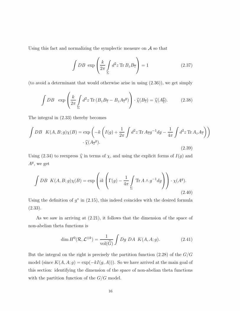
Using this fact and normalizing the symplectic measure on A so that

∫DB exp

k

2π

∫

Σ

d2zTrBzBz

= 1 (2.37)

(to avoid a determinant that would otherwise arise in using (2.36)), we get simply

∫DB exp

k

2π

∫

Σ

d2z Tr (BzBz − BzAzg)

· χ(Bz) = χ(Ag

z). (2.38)

The integral in (2.33) thereby becomes

∫DB K(A,B; g)χ(B) = exp

(−k(I(g) +

1

2π

∫d2zTrAzg

−1dg − 1

4π

∫d2z TrAzAz

))

· χ(Azg).

(2.39)

Using (2.34) to reexpress χ in terms of χ, and using the explicit forms of I(g) and

Ag, we get

∫DB K(A,B; g)χ(B) = exp

ik

Γ(g) − 1

4π

∫

Σ

TrA ∧ g−1dg

· χ(Ag).

(2.40)

Using the definition of g∗ in (2.15), this indeed coincides with the desired formula

(2.33).

As we saw in arriving at (2.21), it follows that the dimension of the space of

non-abelian theta functions is

dimH0(R,L⊗k) =1

vol(G)

∫Dg DA K(A,A; g). (2.41)

But the integral on the right is precisely the partition function (2.28) of the G/G

model (since K(A,A; g) = exp(−kI(g, A))). So we have arrived at the main goal of

this section: identifying the dimension of the space of non-abelian theta functions

with the partition function of the G/G model.

16

Inclusion Of Marked Points

Now we would like to extend the analysis slightly to the case of a Riemann

surface Σ with marked points labeled by representations of G. The G/G model

in this situation will give a path integral representation of the Verlinde algebra.

(This generalization might be omitted on a first reading.)

Suppose one has a represention ρ of a compact Lie group G in a Hilbert space

H. Then as in (2.20), the projection operator onto the invariant subspace of H is

Π =1

vol(G)

∫

G

Dg ρ(g), (2.42)

withDg an invariant measure onG and vol(G) the volume ofG computed with that

measure. The trace of Π is the multiplicity with which the trivial representation

of G appears in H.

Now pick an irreducible representation V of G, that is a vector space V in which

G acts irreducibly by g → ρV (g) ∈ Aut(V ). We want a formula for the multiplicity

with which V appears in G. We can reduce to the previous case as follows. Let V

be the dual or complex conjugate representation of G. The multiplicity with which

V appears in H is the same as the multiplicity with which the trivial representation

appears in H⊗ V . So we define the projection operator ΠV onto the G-invariant

subspace of H⊗ V :

ΠV =1

vol(G)

∫Dg ρ(g) ⊗ ρV (g). (2.43)

The multiplicity with which V appears in H is

mult(V ) = Tr ΠV . (2.44)

We want to apply this to the case in which G is replaced by the group G of

gauge transformations of a principal G bundle P → Σ; and H will be, as above,

17

H0(A,L⊗k). The representations we will use will be the following simple ones.

For a point x ∈ Σ, let rx : G → G be the map of evaluation at x. For any

representation ρV : G → Aut(V ) of G, we have the corresponding representation

ρx,V = ρV ◦ rx of G. Pick now points xi ∈ Σ, labeled by representations Vi, and

let V = ⊗iVi with G acting by

ρV = ⊗iρxi,Vi. (2.45)

The conjugate representation is ρV = ⊗iρxi,V i.

We want to find a path integral representation of the multiplicity with which

V appears in H, along the lines of (2.44). To this aim we must calculate

Tr(ρ(g) ⊗ ρV (g)

)= Tr ρ(g) · Tr ρV (g). (2.46)

Here the first factor has a path integral expression; in fact,

Tr ρ(g) =

∫DA K(A,A; g), (2.47)

with K(A,B; g) the kernel introduced in (2.32). The second factor is simply

Tr ρV (g) =∏

i

TrV ig(xi). (2.48)

So we get

mult(V ) = dim(H⊗ V

)G=

1

vol(G)

∫Dg DA exp(−kI(g, A)) ·

∏

i

TrV ig(xi).

(2.49)

The right hand side is usually called the (unnormalized) correlation function,

⟨∏

i

TrV ig(xi)

⟩(2.50)

in the gauged WZW model. (2.50) would be unchanged if all V i are replaced by

Vi; the gauged WZW action has a symmetry (coming from an involution of G that

exchanges all representations with their complex conjugates) that ensures this.

18

Relation To The Verlinde Algebra

Now let us relate this to the Verlinde algebra. Let T be the maximal torus

of G and G/T the quotient of G by the right action of T . For any irreducible

representation V of G, there is a homogeneous line bundle S over G/T such that

H0(G/T,S) is isomorphic to V .

Given marked points x1, . . . , xs on Σ, let A be the symplectic manifold

A = A×s∏

i=1

(G/T )i (2.51)

where (G/T )i is a copy of G/T “sitting” at xi. This is an informal way to say that

the gauge group G (and its complexification GC) acts on (G/T )i by composition

of the evaluation map rxiwith the natural action of G (or GC) on G/T .

If we are given irreducible representations Vi of G, let for each i Si be a ho-

mogeneous line bundle over (G/T )i such that H0((G/T )i,Si) ∼= V i. Define a

homogeneous line bundle L over A by

L = L⊗k ⊗ (⊗iSi) . (2.52)

(In an obvious way, I have identified the line bundles L and Si with their pullbacks

to A.) Then

H0(A, L) = H0(A,L⊗k) ⊗(⊗iV i

). (2.53)

The multiplicity mult(V ) of (2.49) is therefore the same as the dimension of the

G-invariant subspace of H0(A, L):

mult(V ) = dim(H0(A, L)G

). (2.54)

On the other hand, let R be the quotient of A by GC (the quotient being taken

in the sense of geometric invariant theory, using the ample line bundle L). R is

19

called the moduli space of holomorphic bundles over Σ with parabolic structure,

the parabolic structure being a reduction of the structure group to T at the marked

points xi. (By a theorem of Mehta and Seshadri [28], R coincides with the moduli

space of flat connections on P → Σ −{xi} with certain branching about the xi, up

to gauge transformation.) The GC-invariant line bundle L → A descends to a line

bundle over R, which we will also call L, whose sections over an open set U ⊂ Rare G-invariant sections of L over the inverse image of U in A. So in particular

H0(R, L) = H0(A, L)G. (2.55)

Both R and L depend on the Vi, but I will not indicate this in the notation.

The left hand side of (2.55) is the space of non-abelian theta functions with

parabolic structure. If we combine (2.49), (2.50), (2.54), and (2.55), we find that

the dimension of this space is naturally written as a correlation function in the

gauged WZW model:

dimH0(R, L) =

⟨s∏

i=1

TrVig(xi)

⟩. (2.56)

The Verlinde Algebra

As a special case of this, the Verlinde algebra is defined as follows. For given

“level” k, the loop group of the compact Lie group G has a finite number of

isomorphism classes of unitary, integrable representations; their highest weights

are a distinguished list of isomorphism classes Vα, α ∈ W of representations of

G. Let X be the Z module freely generated by the Vα. X has a natural metric

given by g(Vα, Vβ) = 1 if Vα = V β and otherwise g(Vα, Vβ) = 0. It also has a

natural multiplication structure that we will describe presently. X endowed with

this structure is called the Verlinde algebra.

Using the metric on X, a multiplication law Vα · Vβ =∑

γ NαβγVγ can be

defined by giving a cubic form Nαβγ which is interpreted as∑

δ gγδNαβδ. Such a

cubic form is defined as follows.

20

Take Σ to be a curve of genus zero with three marked points xi, i = 1 . . . 3,

labeled by integrable representations Vαi, αi ∈ W . The choice of the αi and of a

level k determines a moduli space R of parabolic bundles with a line bundle L.

The structure constants of the Verlinde algebra are

Nα1,α2,α3= dimH0(R, L). (2.57)

So in other words, from (2.56), the Verlinde structure functions are the genus zero

three point functions of the G/G model:

Nα1,α2,α3=

⟨3∏

i=1

TrVig(xi)

⟩. (2.58)

The basic phenomenon under study in the present paper is a relation between

the quantum cohomology of the Grassmannian and the G/G model; the result can

be applied to the Verlinde algebra because of (2.58). The special case of a genus

zero surface with three marked points is fundamental because the general case can

be reduced to this by standard sewing and gluing arguments. In fact, such sewing

and gluing arguments, applied to a genus zero curve with four marked points, yield

the associativity of the Verlinde algebra.

Higher Cohomology

Obviously, the above discussion has only a physical level of rigor. Among many

points that should be clarified I will single out one.

If the Vi are integrable representations at level k, then the higher cohomology

H i(R, L), i > 0 vanishes, and dimH0(R, L) coincides with the Euler characteristic

χ(R, L) =∑

i(−1)i dimH i(R, L). From comments made to me by R. Bott and G.

Segal, it appears that for (2.56) to hold for arbitrary representations Vi (perhaps

not integrable), one must replace dimH0(R, L) by χ(R, L). A rigorous treatment

of the G/G model should show the restriction to integrable representations in

deriving (2.56); there may also be a supersymmetric version of the derivation that

naturally gives the Euler characteristic and holds for all representations.

21

2.5. Some Additional Properties

The reader may wish at this stage to turn to §3. However, I will pause here

and in §2.6 below to explain a few additional facts that have their own interest

and will be needed at a few points in §4.

Topological Field Theory

First of all, the gauged WZW theory of G/H is in general conformally invariant

but not topologically invariant. A conformal structure appears in the definition of

the Lagrangian. However, for H = G we have evaluated the partition function of

the G/H model, and found it to be an integer, independent of the conformal struc-

ture of Σ, and equal to the dimension of the space of non-abelian theta functions.

This strongly suggests that the G/G model is actually a topological field theory.

Let us try to demonstrate that directly.

A conformal structure on Σ can be specified by giving a metric h, uniquely

determined up to Weyl scaling. Under a change in h, the change in the G/G

Lagrangian is

δL =k

8π

∫

Σ

d2z√h(hzz)2

(δhzz Tr(g−1Dzg)

2 + δhzz Tr(Dzg · g−1)2). (2.59)

Though this expression does not vanish identically, it vanishes when the classical

equations of motion are obeyed. In fact, under a variation of the connection A,

the Lagrangian changes by

δ′L =k

2π

∫

Σ

d2z√hhzz Tr

(δAzg

−1Dzg − δAzDzg · g−1). (2.60)

So the classical Euler-Lagrange equations, asserting the vanishing of δ′L, are

0 = g−1Dzg = Dzg · g−1. (2.61)

Since (2.59) vanishes when (2.61) does, the G/G model is classically a topological

field theory. Quantum mechanically the analog of using the equations of motion

22

is to make a suitable change of variables in the path integral. In this case, we

consider the infinitesimal redefinition of A

δAz =1

4δhzzh

zzDzg · g−1

δAz = −1

4δhzzh

zzg−1Dzg.

(2.62)

(This is a complex change of coordinates that entails an infinitesimal displacement

of the integration contour in the complex plane, or more exactly a displacement

of the cycle of integration in the complexification of A.) Substituting in (2.61),

we see that the Lagrangian L(g, A) is invariant under a change of metric on Σ

compensated by the transformation (2.62) of the field variables. The path integral

for the partition function

∫Dg DA exp(−L(A, g)) (2.63)

is therefore invariant under the combined change of metric and integration variable,

provided the measure DA is invariant. To this effect, we must compute a Jacobian

or, at the infinitesimal level, the divergence of the vector field that generates the

change of variables (2.62). This is formally

∫

Σ

(δ

δAz(x)δAz(x) +

δ

δAz(x)δAz(x).

)(2.64)

This vanishes, as δAz is indepependent of Az and δAz is independent of Az . This

completes the explanation of why the G/G model is a topological field theory.

Let us note now that the other Euler-Lagrange equation of motion, obtained

by varying with respect to g, is

Dz(g−1Dzg) + Fzz = 0, (2.65)

with F the curvature of the connection A. So given (2.61), this implies that

F = 0. (2.66)

23

Comparison To The Obvious Topological Field Theory

If the goal were to construct a topological field theory using the fields g, A, the

more obvious way to do it would be to take the Lagrangian to be simply

L′(g, A) = −ikΓ(g, A), (2.67)

which manifestly corresponds to a topological field theory, since it is defined with-

out use of any metric or conformal structure. How does this theory compare to

the G/G WZW model?

More generally, let us consider the family of theories

Lk′(g, A) = − k′

8π

∫

Σ

Tr g−1dAg ∧ ∗g−1dAg − ikΓ(g, A), (2.68)

with positive k′. This coincides with the G/G model at k′ = k, and with the

manifestly topologically invariant model at k′ = 0. It is straightforward to work

out that the classical equations of motion are

0 = g−1Dzg − λDzg · g−1 = Dzg · g−1 − λg−1Dzg, (2.69)

with

λ =k′ − k

k′ + k. (2.70)

For 0 < k′ <∞, one has

−1 < λ < 1. (2.71)

(2.69) implies

dAg = 0. (2.72)

For instance, the first equation in (2.69) is equivalent to

(1 − λAd(g)) (Dzg) = 0, (2.73)

with Ad(g)(x) = gxg−1. Since |Ad(g)| ≤ 1 and |λ| < 1, (2.73) implies Dzg = 0,

and similarly (2.69) implies Dzg = 0.

24

Given that (2.72) follows from the classical equations of motion, the same

sort of reasoning as above shows that the Lagrangians Lk′ describe a family of

topological field theories: a change of metric can be compensated by a change of

integration variable with trivial Jacobian.

Now, to study the k′ dependence, look at

∂Lk′

∂k′= − 1

8π

∫

Σ

Tr(g−1dAg ∧ ∗g−1dAg). (2.74)

By virtue of (2.72), this expression vanishes by the classical equations of motion,

so classically the family of theories governed by Lk′ is constant.

From the above discussion, we know how we should proceed quantum mechan-

ically: we should find a change of integration variable that compensates for the k′

dependence of the Lagrangian. Such a change of variable exists because of (2.72);

one can take explicitly

δAz = − δk′

k + k′(1 − λAd(g−1)

)−1(Dzg · g−1). (2.75)

Now, however, a difference arises from our earlier discussion. Because δAz is a

function of Az, the Jacobian of the transformation in (2.75) is not necessarily 1;

the integration measure in the path integral may not be invariant. The change of

the integration measure is formally

∫

Σ

Trδ

δAz(x)δAz(x). (2.76)

Since

δ

δAz(x)δAz(y) ∼ δ2(x, y), (2.77)

this is ill-defined, proportional to δ2(0). In any event, since (2.76) is the integral

over Σ of a local quantity, any regularization should be of that form. Quantities

25

analogous to (2.76) are regularized (albeit in a slightly ad hoc fashion) in [5], in

deriving eqn. (6.22). I will not repeat such a calculation here, but I will just

explain what general form the answer must have, by asking what is the most

general possible perturbation of the G/G model.

The Complete Family Of Theories

Let us simply go back to the gauged WZW model of G/G, and ask what kind of

perturbations it has (see also [29]). We permit the perturbation of the Lagrangian

to be the integral of an arbitrary local functional of g, A, and a metric h on Σ.

In this way we will obtain continuous perturbations of the G/G model, but forbid

discrete perturbations (notably changes in k) that cannot be described via the

addition of a local functional to the Lagrangian.

Perturbations that vanish by the classical equations of motion are irrelevant,

since they can be eliminated by a change of integration variables as described above.

(Even if the integration measure is not invariant under the change of variables,

changes of variables can be used to eliminate the perturbations that vanish by the

equations of motion in favor of other perturbations that do not so vanish.) In

classifying perturbations, we therefore can work modulo operators that vanish by

the classical equations of motion. Given (2.61) and (2.66), this means that we can

discard anything proportional to dAg or F .

The gauge invariant local operators, modulo operators that vanish by the equa-

tions of motion, are generated by operators of the form U(g), with U some function

on G that is invariant under conjugation. Since U(g) is a zero-form, to construct

from it a perturbation of the Lagrangian, we need also a metric h on Σ, or at least

a measure µ, such as the Riemannian measure. The curvature scalar of h will be

called R. The most interesting perturbations are

QU =

∫

Σ

dµ U(g) (2.78)

26

and

SU =

∫

Σ

d2z√hR U(g). (2.79)

(2.78) breaks the diffeomorphism invariance of the G/G model down to in-

variance under the group of diffeomorphisms that preserve the measure µ. The

G/G model perturbed as in (2.78) is an interesting family of theories invariant un-

der area-preserving diffeomorphisms (and reducing for k → ∞ to two dimensional

Yang-Mills theory, which has the same invariance).

Slightly less obviously, the G/G model perturbed by (2.79) is still a topological

field theory. In fact, under an infinitesimal change in h,√hR changes by a total

derivative (so that∫Σ d

2z√hR is a topological invariant, a multiple of the Euler

characteristic). After integrating by parts, the change in (2.79) under a change in

h is

δSU ∼∫

Σ

d2z√h(δhi′j′ − hi′j′h

klδhkl

)hi′ihj′jDiDjU(g). (2.80)

This vanishes by the equations of motion, since dA(g) = 0 implies dU = 0. Hence

one can compensate for δSU with a redefinition of A (and the Jacobian for the

transformation is trivial, since the requisite δA is independent of A).

Other perturbations, such as∫Σ d

2z√hR2U(g), are less interesting, since (i)

they do not possess the large invariances of the theories perturbed by QU or SU ;

(ii) they vanish as a negative power of t if the metric of Σ is scaled up by h→ th,

t >> 1. The latter property means that in most applications of these systems,

such perturbations (if not prevented by (i)) can be conveniently eliminated.

Since the most general perturbation of the G/G model that preserves the dif-

feomorphism invariance is of the form of SU , the regularized version of (2.76) must

be equivalent to SU for some U . By the same token, for any k′, the G/G model

must be equivalent to the Lk′ model perturbed by some SU (with a k′-dependent

U), and vice-versa. In particular, setting k′ = 0, the G/G model is equivalent

27

to the manifestly topologically invariant model with Lagrangian −ikΓ(g, A), per-

turbed by some SU . The requisite U ’s in these statements can in fact be computed

at least heuristically along the lines of the derivation of eqn. (6.22) of [5], but I

will not do so here.

Interpretation

Note that the conjugation-invariant function U(g) that entered above can be

expressed as a linear combination of the characters TrV g, as V runs over irre-

ducible representations of G. These are precisely the operators whose correlation

functions were interpreted algebro-geometrically in (2.56), so the theories obtained

by perturbing the G/G model are all computable in terms of the Verlinde algebra.

2.6. Abelianization

I will now briefly describe another interesting facet of the G/G model, intro-

duced in [5], which apart from its beauty will enter at a judicious moment in §4.⋆

A recurring and significant theme in the theory of compact Lie groups is the

reduction to the maximal torus T , extended by the Weyl group W . As explained in

[5], the G/G model admits such an reduction to the maximal torus. It is equivalent

to the T/T model (that is, the G/H model with both G and H set equal to T )

perturbed by SU , where U is a certain Weyl-invariant function on T and SU is

defined in (2.79).

At the level of precision explained in [5], the abelianization of the model pro-

ceeds as follows. Pick a maximal torus T ⊂ G, with Lie algebra t. Impose the

“gauge condition” g ∈ T .†

Decompose the connection as A = A0 + A⊥, where A0

⋆ A computation reaching a rather similar conclusion is sketched in [4], but unfortunatelythe fermionic symmetry δ introduced in equations (71)-(74) of that paper does not obeyδ2 = 0, which would be needed to justify the computation. I will therefore concentrate onsketching the argument of [5].

† This is not really valid globally as a gauge condition. One must think in terms of integratingover the fibers of the map G→ T/W that maps a group element to its conjugacy class.

28

is the part of the connection valued in t, and A⊥ is valued in the orthocomplement

t⊥ of t. In this gauge the G/G Lagrangian takes the form

LG/G(g, A) = LT/T (g, A0) −k

2π

∫

Σ

d2zTr(A⊥,zA⊥,z − A⊥,zgA⊥,zg

−1). (2.81)

Here

LT/T (g, A0) = kIT/T (g, A0) (2.82)

is the Lagrangian of the T/T model, at level k. The G/G model, in this gauge,

differs from the T/T model by the last term in (2.81), which involves A⊥. To

reduce the G/G model to something like the T/T model, one must “integrate out”

A⊥ to reduce to a description involving g and A0 only. Happily, the A⊥ integral is

Gaussian:

∫DA⊥ exp

k

2π

∫

Σ

d2zTr(A⊥,zA⊥,z − A⊥,zgA⊥,zg

−1) . (2.83)

Such a Gaussian integral formally gives rise to a determinant (as we briefly explain

in §3.5 below). In comparing the G/G model to the T/T model, another determi-

nant arises: the Fadde’ev-Popov determinant comparing the volume of G to the

volume of T . These two determinants are rather singular but at the same time ex-

tremely simple, because the exponent in (2.83) (like the corresponding expression

in the Fadde’ev-Popov determinant) is a local functional without derivatives. In [5],

Blau and Thompson calculate these determinants, with a plausible regularization,

and argue that the G/G model is equivalent to a T/T model with Lagrangian

LT/T (g, A0) = (k + ρ)I(g, A0) −1

4π

∫

Σ

d2x√hR log det t⊥(1 − Ad(g)). (2.84)

Here ρ is the dual Coxeter number of G, and dett⊥(1−Ad(g)) is the determinant of

1−Ad(g), regarded as an operator on t⊥. (This well-known Weyl-invariant function

29

enters in the Weyl character formula, where it has a somewhat similar origin,

involving a comparison of the volumes of G and T .) In §4.6, we will have occasion

to use (2.84) for the case that G = U(k). For that case, if g = diag(σ1, . . . , σk), the

eigenvalues of 1−Ad(g) acting on t⊥ are the numbers 1−σiσj−1, for 1 ≤ i, j ≤ k,

i 6= j. Hence the correction term in (2.84) becomes in this case

∆L = − 1

4π

∫

Σ

d2x√hR

∑

i6=j

ln(σi − σj) − (k − 1)∑

i

ln σi

. (2.85)

Given the role of the G/G model in counting non-abelian theta functions, its

reduction to a T/T model is a kind of abelianization of the problem of counting

such functions. In §7.3 of [5], this is pursued further to obtain a completely explicit

count of non-abelian theta functions for G = SU(2). The role of the endpoint

contributions in equation (7.14) of that paper still deserves closer study.

3. The Quantum Cohomology Of The Grassmannian

The Grassmannian G(k,N) is the space of all k dimensional subspaces of a

fixed N dimensional complex vector space V ∼= CN . If we want to make the

dependence on V explicit, we write GV (k,N).

By associating with a k dimensional subspace of V the N − k dimensional

orthogonal subspace of the dual space V ∗, we see that GV (k,N) ∼= GV ∗(N−k,N).

The relation that we will explain here and in §4 between the Verlinde algebra

of U(k) at level (N − k,N)⋆

and the quantum cohomology of G(k,N) therefore

implies that the Verlinde algebra of U(k) at level (N −k,N) coincides with that of

U(N−k) at level (k,N). This is a surprising fact that had been noted earlier. (For

instance, see [30] and [31, p. 212, Proposition (10.6.4)] for k ↔ N−k symmetry of

loop group representations and [32,33] for such symmetry of the Verlinde algebra.)

⋆ That is, at levels N − k and N for the su(k) and u(1) factors in the Lie algebra of U(k).

30

One way to describe G(k,N) is as follows. Let B be the space of all linearly

independent k-plets e1, . . . , ek ⊂ V . A point in B labels a k-plane V with a basis.

The group GL(k,C) acts on B by change of basis, ei →∑

j Wijej , W ∈ GL(k,C).

Since GL(k,C) acts simply transitively on the space of bases of V , upon dividing

by GL(k,C) we precisely forget the basis and therefore

G(k,N) = B/GL(k,C). (3.1)

B is dense and open in the k-fold product CkN = V × V × . . .× V (since the

generic k-plet e1, . . . , ek ⊂ V is a basis of V ), so G(k,N) is a quotient of a dense

open subset of CkN by GL(k,C). In fact, G(k,N) is the good quotient of CkN by

GL(k,C) that would be constructed in geometric invariant theory.

There is also a symplectic version of this, which will be more relevant in what

follows. Pick a Hermitian metric on V so that V k = CkN gets a metric and a

symplectic structure. In linear coordinates φis, i = 1 . . . k, s = 1 . . .N on CkN , the

symplectic form is

ω = i∑

i,s

dφis ∧ dφis. (3.2)

ω is not invariant under GL(k,C), but it is invariant under a maximal compact

subgroup U(k) ⊂ GL(k,C).

To this symplectic action is associated a “moment map” µ from CkN to the

dual of the Lie algebra of U(k), given by the angular momentum functions that

generate U(k) via Poisson brackets. In this case we can take the moment map to

be

µ : (e1, . . . , ek) → {(ei, ej) − δij}. (3.3)

In other words, µ = 0 precisely if the vectors e1, . . . , ek are orthonormal.

31

Every k-plane has an orthonormal basis, unique up to the action of U(k), so

G(k,N) = µ−1(0)/U(k). (3.4)

This is the description of G(k,N) that we will actually use. We will also want to

remember one fact: µ is a quadratic function on the real vector space underlying

CkN . In components,

µij =

∑

s

φisφjs − δij. (3.5)

3.1. Cohomology

Now we need to discuss the cohomology of G(k,N). We begin with the classical

cohomology. Over G(k,N) there is a “tautological” k-plane bundle E (whose fiber

over x ∈ G(k,N) is the k plane in V labeled by x) and a complementary bundle

F (of rank N − k):

0 → E → V ∼= CN → F → 0. (3.6)

Obvious cohomology classes of G(k,N) come from Chern classes. We set

xi = ci(E∗), (3.7)

where ∗ denotes the dual. (It is conventional to use E∗ rather than E, because

detE∗ is ample.) This is practically where Chern classes come from, as G(k,N)

for N → ∞ is the classifying space of the group U(k). It is known that the xi

generate H∗(G(k,N)) with certain relations. The relations come naturally from

the existence of the complementary bundle F in (3.6). Let yj = cj(F∗), and let

ct(·) = 1 + tc1(·) + t2c2(·) + . . .. Then as a consequence of (3.6),

ct(E∗)ct(F

∗) = 1, (3.8)

and H∗(G(k,N)) is generated by the xi, yj with relations (3.8). If one wishes, these

relations can be partially solved to express the yj in terms of the xi (or vice-versa).

32

Now we come to the quantum cohomology, which originally entered in string

theory, where [34] it enters the theory of the Yukawa couplings (which are related

to quark and lepton masses), and in Floer/Gromov theory of symplectic manifolds

[35]. Additively, the quantum cohomology is the same as the classical one, but the

ring structure is different.

Giving a ring structure on W = H∗(G(k,N)) is the same as giving the identity

1 ∈ W and a cubic form

(α, β, γ) =

∫

G(k,N)

α ∪ β ∪ γ. (3.9)

The cubic form determines a metric

g(α, β) = (α, β, 1), (3.10)

and given a metric the cubic form W ×W ×W → C determines a ring structure

W ×W →W .

So I will explain the quantum cohomology ring by describing the quantum

cubic form. To this aim, let Σ be a closed oriented two-manifold (which in string

theory would be the “world-sheet,” analogous to the world-line of a particle). Let

P ∈ Σ. Let W = Maps(Σ, G(k,N)). Evaluation at P gives a map

Wev(P )−→ G(k,N), (3.11)

by which α ∈ H∗(G(k,N)) pulls back to α(P ) = ev(P )∗(α) ∈ H∗(W).

Now pick a complex structure on Σ, and let M ⊂ W be the space of holomor-

phic maps of Σ to G(k,N). We have M = ∪λMλ, with Mλ being the connected

components of M. In the case of the Grassmannian, the components Mλ are

determined by the degree, defined as follows. If η = c1(E∗), which generates

H2(G(k,N),Z), and Φ : Σ → G(k,N) is such that∫Σ Φ∗(η) = d, then Φ is said to

be of degree d. Since detE∗ is ample, holomorphic curves only exist for d ≥ 0.

33

The quantum cubic form is defined as follows (ignoring analytical details and

tacitly assuming that the Mλ are smooth and compact). Let Σ be of genus zero.

Let P,Q,R be three points in Σ. Then for α, β, γ ∈ H∗(G(k,N)), we set

〈α, β, γ〉 =∑

d

e−dr ·∫

Md

α(P ) ∪ β(Q) ∪ γ(R), (3.12)

with r a real parameter.

In what sense does 〈α, β, γ〉 generalize the classical cubic form? One component

of M, namely M0, consists of constant maps Σ → G(k,N). This component is a

copy of G(k,N) itself. Under that identification the evaluation maps at P,Q, and

R all coincide with the identity, so the contribution of M0 to 〈α, β, γ〉 coincides

with the classical cubic form defined as in (3.9). The quantum cubic form differs

from the classical one by contributions of the rational curves of higher degree.

These contributions are small for r >> 0. In practice, for dimensional reasons, for

every given α, β, γ of definite dimension, the sum in (3.12) receives a contribution

from at most one value of d. (This is in marked contrast to the much-studied case

of a Kahler manifold of c1 = 0, where every positive d can contribute to the same

correlation function.) Therefore, no information is lost if we set r = 0, and that is

what we will do in the rest of this section.

It follows from the definition (for any Kahler manifold, not just the Grassman-

nian) that

〈α, β, 1〉 = (α, β, 1) (3.13)

and thus that the classical and quantum metrics coincide. This is equivalent to

the statement that rational maps of positive degree do not contribute to 〈α, β, 1〉.In fact (as 1(R) = 1), the contribution of a component Mλ of positive degree is

∫

Mλ

α(P ) ∪ β(Q). (3.14)

A group F ∼= C∗ acts on CP1 leaving fixed the points P and Q. F acts freely

on Mλ, if Mλ is a component of rational maps of positive degree. The classes

34

α(P ) and β(Q) in the cohomology of Mλ are pullbacks from Mλ/F . Therefore,

on dimensional grounds (3.14) vanishes.

3.2. The Grassmannian

Let us now work out the quantum cohomology ring of the Grassmannian. As a

preliminary, we note that the contribution of a moduli space Md to the quantum

cubic form obeys an obvious dimensional condition: it vanishes unless the sum

of the dimensions of α, β, γ equals the (real) dimension of Md. The component

Md of genus zero holomorphic curves of degree d in G(k,N) has (according to

the Riemann-Roch theorem) complex dimension dimCG(k,N) + dN . The fact

that this depends on d means that the dimensional condition depends on d and

therefore that the quantum cohomology ring is not Z-graded. However, the fact

that the real dimensions are all equal modulo 2N means that the cohomology is

Z/2NZ-graded.

Returning to the relations ct(E∗)ct(F

∗) = 1 that define the cohomology of the

Grassmannian, we see that (as the left hand side is a priori a polynomial in t of

degree N) the classical relations are of dimension 0, 2, 4, . . . , 2N . To a classical

relation of degree 2k, the rational curves of degree d > 0 will add a correction of

degree 2k − 2dN ; this therefore must vanish unless k = N and d = 1. Therefore,

of the defining relations of the cohomology, the only one subject to a quantum

correction is the “top” relation ck(E∗)cN−k(F

∗) = 0, and the correction is an

element of H∗(G(k,N)) of degree 0 and hence simply an integer. So the non-

trivial effect of the quantum corrections will be simply to generate a relation of the

form

ck(E∗)cN−k(F

∗) = a, (3.15)

for some a ∈ Z. Moreover, a is to be computed by examining rational curves in

the Grassmannian of degree 1. We will find that a = (−1)N−k, so the quantum

35

cohomology ring can be described by the relations

ct(E∗)ct(F

∗) = 1 + (−1)N−ktN . (3.16)

This correction has been described previously [36] in the special case of k = 1

(complex projective space). Despite its simple form, the correction has a dra-

matic effect: while the classical cohomology ring is nilpotent (in the sense that

every element of positive degree is nilpotent), the quantum cohomology ring is

semi-simple. This is evident in its Landau-Ginzburg description [12,3,1] which we

consider presently.

Computation Of a

For X a submanifold of G(k,N), let [X] be its Poincare dual cohomology

class. For instance, for p a point in the Grassmannian, [p] is a top dimensional

class, obeying g(1, [p]) = 1. (It does not matter here if the metric g( , ) is defined

using the classical or quantum cubic form, since we have seen that these determine

the same metric.) The definition of the quantum ring structure from the quantum

cubic form is such that a = ck(E∗)cN−k(F

∗) can be computed as

a = 〈ck(E∗), cN−k(F∗), [p]〉. (3.17)

ck(E∗) equals the Poincare dual of the zero locus of a generic section of E∗.

The dual of the exact sequence (3.6) reads

0 → F ∗ → V ∗ → E∗ → 0, (3.18)

with V ∗ a fixed N dimensional complex vector space. The image in E∗ of any fixed

vector w ∈ V ∗ gives a holomorphic section w of E∗. If as before e1, . . . , eN is a

basis of V , and w is the linear form that maps∑N

i=1 riei to r1, then the restriction

of w to E ⊂ V vanishes precisely if E consists only of vectors with r1 = 0. This is

36

a copy of G(k,N − 1) which we will call Xw. Since w has only a simple zero along

Xw (any E can be perturbed in first order to get one for which w 6= 0), we have

ck(E∗) = [Xw]. (3.19)

For future use, let us note that

∫

G(k,N)

ck(E∗)N−k = 1. (3.20)

Indeed, we can pick N − k holomorphic sections of E∗ whose zero sets intersect

transversely at a single point. To do so, let wi for i = 1, . . . , N − k be the linear

form on V that maps∑N

i=1 riei to ri. Then the wi have the required properties,

vanishing precisely for E the k-plane spanned by eN−k+1, . . . , eN .

Now let us compute cN−k(F∗) = (−1)N−kcN−k(F ). Under the holomorphic

surjection V → F , any vector v ∈ V projects to a holomorphic section v of F . v

vanishes precisely if v ∈ E; let Yv = {E ∈ G(k,N)|v ∈ E}. Then v has a simple

zero along Yv, so cN−k(F ) = [Yv] and therefore

cN−k(F∗) = (−1)N−k[Yv]. (3.21)

Rational curves of degree one in G(k,N) can all be described as follows. Let

(s, t) be homogeneous coordinates for CP1. For r1, . . . , rk a set of k linearly in-

dependent vectors in the N dimensional vector space V , let {r1, . . . , rk} be the

k-plane that they span. Then a rational curve of degree one in G(k,N) is of the

form

(s, t) → {sr0 + tr1, r2, r3, . . . , rk}, (3.22)

with r0, . . . , rk being linearly independent vectors in V .

37

We have to calculate

a = (−1)N−k

∫

M1

[Xw](P ) ∪ [Yv](Q) ∪ [p](R). (3.23)

Here M1 is the space of degree 1 rational curves, w ∈ V ∗, v ∈ V , and P,Q,R

are points in CP1. If everything is sufficiently generic, a is simply the number of

degree one curves that pass through Xe at P , through Yf at Q, and through p at

R.

We choose p to be an arbitrary point in G(k,N) corresponding to a k-plane

spanned by vectors v1, . . . , vk. We take v = v0 to be linearly independent of these,

and we pick w to be any linear form that maps v0 to 1, v1 to −1, and the vj of

j > 1 to 0.

From the explicit description of degree one curves in (3.22), we see that the

k-planes represented by points in the image of such a curve are subspaces of a

common k + 1-plane. For a curve that passes through Yv at Q and through p at

R, this is clearly the k + 1-plane W spanned by v0, v1, . . . , vk. Requiring that the

curve pass also through Xw at P determines the curve uniquely. For instance, if

Q = (1, 0), R = (0, 1), and P = (1, 1), then the degree 1 curve must be

(s, t) → {v0s+ v1t, v2, . . . , vk}. (3.24)

The subvarieties [Xw](P ), [Yf ](Q), and [p](R) of M∞ meet transversely at that

point, so we get finally

a = (−1)N−k (3.25)

as claimed above.

38

Landau-Ginzburg Formulation

Write

ct(E∗) =

k∑

i=0

xiti, (3.26)

with xi = ci(E∗). Define functions yj(xi), j ≥ 0 by

1

ct(E∗)=∑

j≥0

yjtj . (3.27)

Classically, the cohomology ring of G(k,N) is described by the relations

yj = 0, for N − k + 1 ≤ j ≤ N. (3.28)

Let

−logct(E∗) =

∑

r≥0

Ur(x1, . . . , xk)tr. (3.29)

So

−tjct(E∗)−1 = − ∂

∂xjlogct(E

∗) =∑

r≥0

∂Ur

∂xjtr. (3.30)

Hence if

W0 = (−1)N+1UN+1 (3.31)

then

∂W0

∂xi= (−1)NyN+1−i, for 1 ≤ i ≤ k. (3.32)

So the defining relations of the classical cohomology take the form

dW0 = 0. (3.33)

39

To obtain in a similar way the quantum cohomology ring, set

W = W0 + (−1)kx1. (3.34)

The relations dW = 0 now give

yN+1−i + (−1)N−kδi,1 = 0. (3.35)

Therefore the relation ct(E∗) · (∑j yjt

j) = 1 becomes

(k∑

i=0

xiti

)·

N−k∑

j=0

yjtj − (−1)N−ktN +O(tN+1)

= 1. (3.36)

Keeping only the terms of order at most tN , this becomes

(k∑

i=0

xiti

)·

N−k∑

j=0

yjtj

= 1 + (−1)N−ktN . (3.37)

This coincides with the quantum cohomology ring as described in (3.16). The

function W is called the Landau-Ginzburg potential.

If we introduce the roots of the Chern polynomial

ct(E∗) =

k∏

i=1

(1 + λit), (3.38)

then W can be written

W (λ1, . . . , λk) =1

k + 1

k∑

j=1

(λj

N+1 + (−1)kλj

). (3.39)

Now let us discuss integration. Integration defines a linear functional on the

top dimensional cohomology of G(k,N), which is the cohomology in real dimension

40

2k(N − k):

f → I(f) =

∫

G(k,N)

f. (3.40)

Since H2k(N−k)(G(k,N)) is one dimensional, any two linear functionals on that

space are proportional. Such a linear functional can be obtained as follows in the

Landau-Ginzburg description. We examine the classical case first. If we consider

xi = ci(E∗) to be of degree i, then the top dimensional cohomology consists of

polynomials f of degree k(N − k) modulo the ideal generated by ∂W0/∂xi, i =

1 . . . k. Consider the linear form on homogeneous polynomials of degree k(N − k)

defined by

J(f) = (−1)k(k−1)/2

(1

2πi

)k ∮dx1 . . . dxk

f∏k

i=1 ∂W0/∂xi

. (3.41)

The integration contour is a product of circles enclosing the poles in the denomi-

nator. J(f) annihilates the ideal generated by dW0, since if f is divisible by, say,

∂W/∂xi, then one of the denominators in (3.41) is canceled and one of the contour

integrals vanishes.

For f of degree k(N − k), the integral in (3.41) is unaffected if W0 is replaced

by W ; this follows from taking the contour integral on (3.41) to be a large contour.

The integral can then be evaluated as a simple sum of residues:

J(f) = (−1)k(k−1)/2∑

dW=0

f

det(

∂2W∂xi∂xj

) . (3.42)

It is convenient to change variables from the xi to the λa. One has

det

(∂2W

∂xi∂xj

)∣∣∣∣dW=0

= det

(∂2W

∂λa∂λb

)· det

(∂λa

∂xi

)2

. (3.43)

The Jacobian in the change of variables from xi to λa is the Vandermonde deter-

41

minant:

det

(∂xi

∂λa

)2

=∏

a<b

(λa − λb)2. (3.44)

So

J(f) =(−1)k(k−1)/2

k!

∑

dW (λa)=0

f ·∏a<b(λa − λb)2

∏a dW/dλa

=(−1)k(k−1)/2

k!(2πi)k

∮dλa

f ·∏a<b(λa − λb)2

∏a dW/dλa

.

(3.45)

The integration contour in each λa integral is a circle running counterclockwise

around the origin. A factor of k! comes here because, as the map from the λa to

the xi is of degree k!, each critical point of W (xi) corresponds to k! critical points

of W (λa).

To verify that J(f) is correctly normalized to coincide with I(f), we set f =

ck(E∗)N−k =

∏a λ

N−ka . According to (3.20), I(f) = 1. To verify that J(f) = 1,

we use the contour integral version of (3.45). In the denominator we can replace

dW/dλa = λaN +(−1)k by λa

N −λaN−k without changing the behavior on a large

contour enough to affect the integral. Then

J(f) =(−1)k(k−1)/2

k!(2πi)k

∮dλ1 . . . dλk

∏a<b(λa − λb)

2

∏c(λ

kc − 1)

. (3.46)

The integral is easily done as a sum of residues. The poles are at λak = 1, for

1 ≤ a ≤ k. Because of the Vandermonde determinant in the numerator, the

λa must be distinct. Up to a permutation, one must have λa = exp(2πia/k);

evaluating the residue at this value of the λa and including a factor of k! from the

sum over permutations, one gets J(f) = 1.

42

3.3. Quantum Field Theory Interpretation

Physicists would never actually begin with the definition that I have given

above for the quantum cubic form. Rather, everything begins with considerations

on the function space W = Maps(Σ, G(k,N)). Physicists are mainly interested in

quantum field theory, which is conveniently formulated in terms of integration over

spaces such as W.

For instance, let Σ be a complex Riemann surface with Hodge duality operator

∗, pick a Hermitian metric on G(k,N) (such as the natural U(k)-invariant metric),

and for a map Φ : Σ → G(k,N), set

L(Φ) =

∫

Σ

(dΦ, ∗dΦ). (3.47)

Then in the “bosonic sigma model with target space G(k,N)” we consider integrals

such as∫

W

DΦ exp

(−L(Φ)

λ

), (3.48)

with λ a positive real number. This is not complete pie in the sky. For instance,

to make the definition more concrete, one can triangulate Σ and make a finite

dimensional approximation to the integral. Then the problem is to adjust λ, while

refining the triangulation, so that the given integral (and related ones) converges

as the triangulation is infinitely refined.

For a homogeneous space of positive curvature such as the Grassmannian, one

knows at a physical level of rigor precisely how to do this: λmust be taken to vanish

in inverse proportion to the logarithm of the number of vertices in the triangulation.

This is a consequence of a phenomenon known as “asymptotic freedom,” which

plays a crucial role in the theory of the strong interactions in four dimensions;

sigma models with targets such as the Grassmannian were intensively studied in

the late 1970’s and early 1980’s as simple cases of asymptotically free quantum

43

field theories. Asymptotic freedom actually plays an important role in our story,

since it leads to the mass gap that will be essential in §4.

Supersymmetric Sigma Models

What we actually want to do is to transfer the integral over the space of

holomorphic maps that defined the quantum cohomology ring,

〈α, β, γ〉 =∑

λ

∫

Mλ

α(P ) ∪ β(Q) ∪ γ(R), (3.49)

to an integral over the space W of all maps of Σ to G(k,N). Reversing the usual

logic, this is done as follows. The condition that Φ : Σ → G(k,N) is holomorphic

is an equation

0 =(∂Φ)1,0

(3.50)

which asserts the vanishing of a section

s : Φ → (∂Φ)1,0 (3.51)

of an infinite dimensional vector bundle Y over W. (Y is the bundle whose fiber

at Φ ∈ W is the space of (0, 1) forms on Σ with values in Φ∗(T 1,0G(k,N)), with

T 1,0G(k,N) being the (1, 0) part of the complexified tangent bundle of G(k,N).

The point of the definition is just that (∂φ)1,0 is a vector in Y .)

The space M of holomorphic maps, being defined by the vanishing of a section

s : W → Y , is Poincare dual to the Euler class χ(Y ) of Y . So formally we can

write

〈α, β, γ〉 =

∫

M

α ∪ β ∪ γ =

∫

W

α ∪ β ∪ γ ∪ χ(Y ). (3.52)

Now, there are any number of ways to write a differential form representing χ(Y ),

but one nice way (formulated mathematically by Mathai and Quillen [37]) uses a

44

section s and has a nice exponential factor exp(−|s|2/λ), with |s|2 the norm of

s with respect to a metric on Y , and λ a positive real number. For the section

indicated in (3.51), the norm with respect to the natural metric is

|s|2 =

∫

Σ

(dΦ, ∗dΦ), (3.53)

which is precisely the Lagrangian introduced above for the bosonic sigma model

with target space the Grassmannian.

So the long and short of it is that we get a representation

〈α, β, γ〉 =

∫

W×...

∫DΦ . . . exp

−1

λ

∫

Σ

|dΦ|2 + . . .

α(P )β(Q)γ(R), (3.54)

much like the bosonic sigma model, but with “fermions,” represented by “. . .”

The quantum field theory that appears here is in fact a twisted form of the usual

supersymmetric nonlinear sigma model, as I explained in [38]; in the twisted model,

the fermions can be interpreted in terms of differential forms on the function space

W. The relation to the Mathai-Quillen formula was explained by Atiyah and

Jeffrey [39] in the analogous case of four dimensional Donaldson theory.

It should be fairly obvious that instead ofG(k,N) we could use a general Kahler

manifold X in the above discussions, at least at the classical level. (If we are willing

to give up the interpretation in terms of twisting of a unitary supersymmetric

model, we can even consider almost complex manifolds that are not Kahler.) At

the quantum level, the situation is more subtle. There are two main branches

in the subject. If c1(X) = 0, the supersymmetric sigma model (with a suitable

choice of the Kahler metric of X) is conformally invariant; such models provide

classical solutions of string theory. On the other hand, if c1 > 0, as in the case of

the Grassmannian, one is in a quite different world, with asymptotic freedom and

analogs of the mass generation and chiral symmetry breaking seen in the strong

interactions.

45

3.4. Strategy

To try to say something of substance in this situation, we use the realization

of G(k,N) as µ−1(0)/U(k), where µ is the moment map from CkN to the Lie

algebra of U(k). One is tempted to try to lift a map Φ : Σ → G(k,N) to a map

Φ : Σ → CkN . There is not a natural way to do this, and there may even be a

topological obstruction.

So instead we proceed as follows. Let P be a principal U(k) bundle over Σ,

A a connection on P , Φ a section of P ×U(k) CkN , and S a two-form on Σ with

values in the adjoint bundle ad(P ). Take

L(Φ, A, S) =

∫

Σ

((dAΦ, ∗dAΦ) + i(S, µ ◦ Φ)

). (3.55)

Then classically the theory described by L(Φ, A, S) is equivalent to the bosonic

sigma model with target G(k,N). This can be seen as follows. The Euler-Lagrange

equation of S is µ ◦ Φ = 0, so, under the natural projection P ×U(k) CkN →CkN/U(k), Φ maps to Φ : Σ → µ−1(0)/U(k) = G(k,N). The Euler-Lagrange

equation for A identifies P and A with the pull-back by Φ of the tautological

principal U(k) bundle and connection over G(k,N). Once these restrictions and

identifications are made, L(Φ, A, S) reduces to the Lagrangian L(Φ) of the bosonic

sigma model of the Grassmannian.

This sort of reasoning is still valid quantum mechanically. For instance, using

∞∫

−∞

dx

2πeixy = δ(y) (3.56)

(and the obvious generalization of that formula to several variables) we get the

path integral formula

∫DS exp

−i

∫

Σ

(S, µ ◦ Φ)

= δ(µ ◦ Φ). (3.57)

46

So the S integral places on Φ precisely the restriction that one would guess from the

classical Euler-Lagrange equations. From simple properties of Gaussian integrals

(which are introduced below), one similarly deduces that, quantum mechanically

as classically, the A integral has the effect of identifying P,A with the pull-backs

of the tautological objects over the Grassmannian.

Similar reasoning holds after including fermions, so we get for the quantum

cubic form a representation of the general kind

〈α, β, γ〉 =

∫DΦDADS . . . exp

−

∫

Σ

((dAΦ, ∗dAΦ) + i(S, µ ◦ Φ) + . . .

)·α(P )β(Q)γ(R).

(3.58)

As before, “. . .” represents terms involving fermions that are not indicated explic-

itly.

3.5. Reversing The Order Of Integration

In sum, (3.58) will reduce to (3.54) if we integrate over A and S first. To get

something interesting, we instead integrate first over Φ. The key point is that Φ

is a section of a bundle over Σ with linear fibers (a CkN bundle) and that L is

quadratic in Φ. Consequently, the Φ integral is a Gaussian integral.

The basic one dimensional formula

∞∫

−∞

dx√2π

exp(−λx2/2) =1√λ

(3.59)

has the n dimensional generalization

∞∫

−∞

dx1 . . . dxn

(2π)n/2exp

−1

2

∑

i,j

Mijxixj

=

1√detM

, (3.60)

for any quadratic form M with positive real part; this is demonstrated by picking

a coordinate system in which M = diag(m1, . . . , mn).

47

In our case the Φ integral is (apart from terms involving fermions)

∫DΦ exp

−

∫

Σ

((dAΦ, ∗dAΦ) + i(S, µ ◦ Φ)

) . (3.61)

This is an infinite dimensional Gaussian integral with M the quadratic form asso-

ciated with the elliptic differential operator

M ′ = (d∗AdA + iS) ⊗ 1N . (3.62)

The notation reflects the fact that the CkN bundle of which Φ is a section is

actually a sum of N copies of a Ck bundle, and M is the sum of N copies of a

quadratic form derived from an operator (namely d∗AdA + iS) on sections of that

Ck bundle. So the integral over Φ gives

1√detM ′

=

(1√

det(d∗AdA + iS)

)N/2

. (3.63)

The determinant of the elliptic differential operator d∗AdA + iS can be conveniently

defined using the ζ-function regularization of Ray and Singer.

So modulo fermions we get

〈α, β, γ〉 =

∫DADS . . .

(1√

det(d∗AdA + iS)

)N/2

· αβγ. (3.64)

So we have transformed the problem of computing the quantum cohomology of the

Grassmannian to a problem involving integration over the connection A and over

S – a problem in quantum gauge theory. This brings us into an entirely different

world, that of §2 of this paper.

As this stage we can see why – as topologists might expect – the sigma model

of G(k,N) simplifies in the limit of k fixed, N → ∞. The integrand in (3.64)

48

has a sharp peak at the minimum of the determinant, and “everything” can be

calculated in an asymptotic expansion in powers of 1/N , by expanding around this

peak.

For fixed N , it is not true that “everything” can be calculated, but the topo-

logical quantities can be, reducing to a saddle point by a more elaborate argument.

The essence of the matter is that although the classical Lagrangian L is confor-

mally invariant, the quantum theory is not (because, for instance, with Ray-Singer

or any other regularization, the determinant introduced above is not conformally

invariant). The topological quantities are however not just conformally invariant

but completely independent of the metric of Σ. Scaling up the metric of Σ by

a very large real factor, life simplifies because of the basic physical properties of

the model – asymptotic freedom and the dynamically generated mass gap. At

very large distances (that is, if the metric on Σ is scaled up by a very big factor),

the complicated integral over A, S, and fermions in (3.64) reduces to a local and

tractable quantum field theory – in fact it reduces to the gauged WZW model (of

U(k)/U(k)) that was analyzed in §2.

There is a basic principle here: every quantum field theory with a mass gap

reduces at very big distances to a topological field theory. Often the topological

field theory that so arises is more or less trivial, but in the case of the supersym-

metric sigma model of the Grassmannian, it is the gauged WZW model. This large

distance reduction of the Grassmannian sigma model to a gauged WZW model,

plus the relation explained in §2 between the gauged WZW model and the Verlinde

algebra, give the relation between the quantum cohomology of the Grassmannian

and the Verlinde algebra.

It is well known that at large distances, massive particles can be neglected and

massless particles dominate. Less fully appreciated is that beyond the reach of the

propagating fields, a non-trivial dynamics of the vacuum or topological field theory

may prevail.

49

Differential Geometry Of The Moduli Space Of Bundles

A detailed discussion of the reduction of the sigma model to the gauged WZW

model will be the subject of §4, but here I will make a few naive remarks. The

integrand in (3.64) actually has its maximum for flat connections – with some

branching at the points P,Q,R ∈ Σ at with α, β, and γ are inserted. The moduli

space of such flat connections is (by a theorem of Mehta and Seshadri [28]) the same

as the moduli space R of rank k stable holomorphic vector bundles over Σ, with

some parabolic structure at P,Q,R determined by the branching. So the integral

gives some differential geometry of R. (In view of (2.66), R can be interpreted as a

space of classical solutions of the gauged WZW model.) In the large N limit, direct

analysis of the determinant in (3.64) shows that the differential geometric quantity

that appears is the volume of the symplectic manifold R, times NdimC R. This is

the leading large N behavior of the Riemann-Roch formula for the dimension of the

space H0(R,LN−k) of non-abelian theta functions. This simple direct argument

relates the quantum cohomology of G(k,N) to the dimension of the space of non-

abelian theta functions for large N .

The only way I know to establish this as an exact relation, not just as asymp-

totic one for large N , is to reduce the sigma model of G(k,N) to the gauged WZW

model as we will do in §4, and then study that model as in §2.

4. From The Grassmannian To The G/G Model

This section is organized as follows. After recalling some background about

N = 2 models in two dimensions in §4.1, we construct in §4.2 the sigma model

whose target space is the Grassmannian G(k,N). Then we analyze its behavior

at long distances in §4.3-6. In §4.7-8, we enter the computational stage and work

things out in detail in the simplest non-trivial case.

In the past, the long distance behavior of the Grassmannian sigma model has

been analyzed on R2 [7–10]; the main results were spontaneously broken chiral

50

symmetry, the existence of a mass gap, and a determination for large N of the

spectrum of low-lying states. The novelty here is to examine the long distance

behavior more globally, uncovering the relation to the gauged WZW model and

thereby (in view of §2) the Verlinde algebra.

I will make a small change in notation in this section. In §2, we considered

general compact Lie groups, and (as is conventional in mathematics) we took the

Lie algebra to consist of anti-hermitian matrices (so the quadratic form (a, b) =

Tr ab is negative definite). The reason that this convention is standard for general

Lie groups is that in the case of a real group, whose representations may also all

be real, it is unnatural to introduce factors of i and therefore the group generators

are naturally anti-hermitian. In this section, the gauge group will be the unitary

group U(k), which will arise in a natural complex representation, and I will follow

the standard physics convention that the group generators are hermitian matrices;

thus (a, b) = Tr ab will be positive definite. The complexification of the Lie algebra

of U(k) consists of all k × k complex matrices; if σ is such a matrix, then σ will

denote its hermitian adjoint.

4.1. Background

We will work in N = 2 superspace in two dimensions, conventions and the

basic setup being as explained in [40,41]. The detailed formulas of this subsection

are presented mainly for reference, and most readers will want to skim them.

We consider first flat superspace with bosonic coordinates xm, m = 0, 1 (and

Lorentz signature −+) and fermionic coordinates θα, θα. In a light-cone basis,

supersymmetry is realized geometrically by the operators

Q± =∂

∂θ±+ iθ

±(

∂

∂x0± ∂

∂x1

)

Q± = − ∂

∂θ± − iθ±

(∂

∂x0± ∂

∂x1

).

(4.1)

51

These operators commute with the superspace covariant derivatives

D± =∂

∂θ±− iθ

±(

∂

∂x0± ∂

∂x1

)

D± = − ∂

∂θ± + iθ±

(∂

∂x0± ∂

∂x1

) (4.2)

which are used in constructing Lagrangians.

To formulate gauge theory, one introduces a gauge field in superspace, replacing

the differential operators Dα, Dα, and ∂m = ∂/∂xm by gauge covariant derivatives

Dα, Dα, and Dm. On the superspace gauge fields one imposes the very strong

constraints

0 = {Dα,Dβ} = {Dα,Dβ}{D±,D±} = 2i (D0 ±D1) .

(4.3)

Among other things, these conditions permit the existence of “chiral superfields,”

superspace fields Φ obeying

DαΦ = 0. (4.4)

With the aid of the constraints one can take locally

Dα = e−VDαeV

Dα = eVDαe−V

(4.5)

where V is a real Lie algebra-valued function on superspace, called a vector su-

perfield. After also fixing some residual gauge invariance, one can go to a “Wess-

Zumino gauge,” in which

V = θ−θ−(v0 − v1) + θ+θ

+(v0 + v1) −

√2σθ−θ

+ −√

2σθ+θ−

+ 2iθ−θ+(θ−λ− + θ

+λ+

)+ 2iθ

+θ−(θ+λ+ + θ−λ−) + 2θ−θ+θ

+θ−D.

(4.6)

Here vm is an ordinary two-dimensional gauge field, and the other fields are bose

and fermi matter fields. σ is a complex k × k matrix, and – as V is hermitian –

52

sigma is its hermitian adjoint. We write F = F01 = ∂0v1 − ∂1v0 + [v0, v1] for the

curvature of v. The supersymmetry transformation laws for this multiplet are

δvm = iǫσmλ+ iǫσmλ

δσ = −i√

2ǫ+λ− − i√

2ǫ−λ+

δσ = −i√

2ǫ+λ− − i√

2ǫ−λ+

δD = −ǫ+(D0 −D1)λ+ − ǫ−(D0 +D1)λ− + ǫ+(D0 −D1)λ+ + ǫ−(D0 +D1)λ−

+√

2ǫ+[σ, λ−] +√

2ǫ−[σ, λ+] +√

2[σ, λ+]ǫ− +√

2[σ, λ−]ǫ+

δλ+ = iǫ+D +√

2(D0 +D1)σǫ− − F01ǫ+ − [σ, σ]ǫ+

δλ− = iǫ−D +√

2(D0 −D1)σǫ+ + F01ǫ− + [σ, σ]ǫ−

δλ+ = −iǫ+D +√

2(D0 +D1)σǫ− − F01ǫ+ + [σ, σ]ǫ+

δλ− = −iǫ−D +√

2(D0 −D1)σǫ+ + F01ǫ− − [σ, σ]ǫ−.(4.7)

The basic gauge invariant field strength is

Σ =1

2√

2{D+,D−} = σ + i

√2θ+λ+ − i

√2θ

−λ− +

√2θ+θ

−D

− iθ−θ−(D0 −D1)σ − iθ+θ

+(D0 +D1)σ

+√

2θ−θ−θ+(D0 −D1)λ+ −

√2θ+θ

+θ−(D0 +D1)λ− − i

√2θ+θ

−F01

− 2iθ−θ−θ+[σ, λ−] − 2iθ

−θ+θ

+[σ, λ+]

− θ−θ−θ+θ

+ ((D0

2 −D12)σ − [σ, [σ, σ]]

)+ iθ−θ

−θ+θ

+[σ, ∂mv

m].(4.8)

(The last term does not really spoil gauge invariance: the gauge transformations

that preserve Wess-Zumino gauge have a certain θ dependence which requires this

term to be present.) Σ is a twisted chiral superfield; this means that (by the

Bianchi identity together with the constraints)

D+Σ = D−Σ = 0. (4.9)

With the aid of Σ, it is straightforward to construct gauge invariant La-

53

grangians. The standard gauge kinetic energy is

Lg = − 1

4e2

∫d2x d4θTr ΣΣ

=1

e2

∫d2x Tr

(1

2F 2

01 + |D0σ|2 − |D1σ|2 + iλ−(D0 +D1)λ− + iλ+(D0 −D1)λ+

+1

2D2 − 1

2[σ, σ]2 −

√2λ+[σ, λ−] +

√2[σ, λ−]λ+

).

(4.10)

One more term constructed from gauge fields only is important. Using the fact

that Σ is a twisted chiral superfield, there is an invariant interaction of the form

LD,θ =it

2√

2

∫d2x dθ+ dθ

−Tr Σ|

θ−=θ+=0

+ c.c. =

∫d2x

(−rTrD +

θ

2πTrF01

),

(4.11)

with

t = ir +θ

2π. (4.12)

Matter Fields

Chiral superfields are functions Φ on superspace, transforming in some given

unitary representation V of the gauge group, and obeying

D±Φ = 0. (4.13)

Such a field has an expansion in components

Φ = φ+√

2θαψα + θαθαF. (4.14)

The supersymmetry transformation laws for this multiplet are (by dimensional

54

reduction from [40, p. 50])

δφ =√

2 (ǫ+ψ− − ǫ−ψ+)

δψ+ = i√

2 (D0 +D1)φǫ− +√

2ǫ+F − 2σφǫ+

δψ− = −i√

2 (D0 −D1)φǫ+ +√

2ǫ−F + 2σφǫ−

δF = −i√

2ǫ+ (D0 −D1)ψ+ − i√

2ǫ− (D0 +D1)ψ−

+ 2 (ǫ+σψ− + ǫ−σψ+) + 2i(ǫ−λ+ − ǫ+λ−

)φ.

(4.15)

The usual kinetic energy for a multiplet of such chiral superfields is

Lch =1

4

∫d2x d4θ ΦΦ =

∫d2x

(|D0φ|2 − |D1φ|2 + |F |2 + iψ+(D0 −D1)ψ+

+iψ−(D0 +D1)ψ− + φDφ− φ{σ, σ}φ−√

2ψ+σψ− −√

2ψ−σψ+ + i√

2ψ+λ−φ− i√

2ψ−λ+φ

+i√

2φλ+ψ− − i√

2φλ−ψ+

).

(4.16)

The |Dαφ|2 term in (4.16) is the conventional free kinetic energy corresponding

to a sigma model with a flat metric on V ∼= Cr. The φDφ term is the coupling of

D to the moment map, in the sense that if we pick a basis Ta, a = 1 . . .dimG for

the Lie algebra of G, then this term is

∫d2x

∑

a

Da(φ, Taφ), (4.17)

and the functions (φ, Taφ) are the components of the moment map.

A more general Kahler metric on V (and accordingly, a more general form of

the moment map) could be obtained by replacing the function ΦΦ on the left hand

side of (4.16) with a more general Kahler potential K(Φ,Φ). These matters are

explained in some detail in [42].

55

4.2. The Model

Now we can construct the actual model of interest. We take the gauge group to

be G = U(k). We take kN chiral superfields Φis, i = 1 . . . k, s = 1 . . .N , regarded

as N copies of the defining k dimensional representation of G. The action of G

commutes with a global symmetry group H ∼= U(N) which one can think of as the

unitary transformations of CN .

The Lagrangian that we actually wish to study is simply

L = Lgauge + LD,θ + Lch. (4.18)

The potential energy is determined by the following terms in L:

Lpot =1

2e2TrD2 − rTrD + φDφ− 1

2e2Tr[σ, σ]2 − φ{σ, σ}φ. (4.19)

Upon integrating out D, the potential energy is

V =e2

2

k∑

i,j=1

(∑

s

φisφjs − δi

jr

)2

+1

2e2Tr[σ, σ]2 + φ{σ, σ}φ. (4.20)

The space of classical vacua is the space of zeroes of V up to gauge transfor-

mation. For V to vanish, φ must be non-zero, and therefore σ must vanish. As

anticipated in §3, the first term in the potential is the square of the moment map

for the action of U(k) on CkN . This term vanishes precisely if the vectors in CN

represented by the rows of φ, divided by√r, are orthonormal. The k dimensional

subspace V ⊂ CN spanned by the rows of φ is gauge invariant, and is the only

gauge invariant data determined by φ (since any two orthonormal bases of V are

related by the action of U(k)). Moreover, every k dimensional subspace V ⊂ CN

has such an orthonormal basis. So the space of classical vacua is the Grassmannian

G(k,N) of k dimensional subspaces of CN .

56

Since the condition for vanishing energy is

∑

s

φisφjs = δi

jr, (4.21)

the radius of the space of vacua is√r and the Kahler class is proportional to r.

Classically, the space of vacua shrinks to a point for r = 0; for r < 0 the classical

energy can no longer vanish and it appears that supersymmetry is spontaneously

broken. Quantum mechanically, the situation is rather different and there is a

smooth continuation to negative r with unbroken supersymmetry, as discussed

(for k = 1) in [41,§3.2]; the existence of this continuation will be exploited below.

The choice of a classical vacuum spontaneously breaks the symmetry group

U(N) to U(k) × U(N − k), while leaving supersymmetry unbroken. The oscilla-

tions in the vacuum are massless Goldstone bosons at the classical level. Their

supersymmetric partners are, of course, also massless classically. Other modes

are readily seen to have masses proportional to e. The model therefore reduces

at long distances (or equivalently for e → ∞) to the supersymmetric nonlinear

sigma model with target space the Grassmannian; we will more briefly call this the

Grassmannian sigma model.

At the quantum level, spontaneous breaking of a continuous symmetry such

as the U(N) symmetry of this model is not possible in two dimensions. The

symmetry must therefore be restored by quantum corrections. Exhibiting this

symmetry restoration, and the associated mass gap, was a primary goal of early

investigations of the model.

R Symmetries

A right-moving R-symmetry in an N = 2 model in two dimensions is a sym-

metry under which θ+ → eiαθ+, θ+ → e−iαθ

+, while θ−, θ

−are invariant. A

left-moving R-symmetry obeys the analogous condition with θ+ and θ− exchanged.

The Grassmannian sigma model as constructed above has at the classical level

57

a right-moving R-symmetry JR⋆

under which the charges of the various fields

are as follows: (ψ+, F, σ, λ−) have charges (−1,−1, 1, 1), their complex conju-

gates have opposite charge, and other fields have charge zero. Similarly there is

classically a left-moving R-symmetry JL under which (ψ−, Fi, σ, λ+) have charges

(−1,−1,−1, 1), their complex conjugates have opposite charges, and other fields

are neutral.

At the quantum level, the sum JV = JR + JL is a “vector” symmetry, that is,

it transforms left- and right-moving fermions the same way, so it is free of anomaly

and generates a U(1) symmetry.

However, the “axial” combination JA = JR − JL is anomalous. The anomaly

can be described as follows. Let a be a U(1) connection with first Chern class 1, and

embed this in G = U(K) so that the U(k) gauge field is v = diag(a, 0, 0, . . . , 0).

In such an instanton field, the index of the Dirac operator acting on ψ+ is N .†

Similarly the ψ− index is −N . The total anomaly in JA = JR−JL is the difference

of these or 2N . The anomaly in any instanton field would be an integer multiple

of this.

So JA is conserved only modulo 2N . The only symmetries we can construct

from JA are the discrete transformations exp(2πitJA/2N), with t ∈ Z. This gives

a discrete group, isomorphic to Z2N , of chiral symmetries. If unbroken, these

symmetries would prevent ψ and λ from gaining a mass. One of the main results

of the old literature on this model was that this Z2N is spontaneously broken down

to Z2, making a mass gap possible; the surviving Z2 is just the operation (−1)F

that counts fermions modulo two.

The Twisted Model

Any N = 2 supersymmetric theory in two dimensions with an R symmetry

⋆ We will somewhat imprecisely use the symbol JR to denote either the current or the corre-sponding charge; and similarly for other currents introduced momentarily.

† The index is defined as the number of ψ+ zero modes minus the number of ψ+ zero modes.Recall that ψ+ transforms as a sum of N copies of the defining k-dimensional representationof U(k); each of these contributes 1 to the index.

58

can be twisted to obtain a topological field theory. The construction, as explained

in [43], which the reader can consult for details, involves adding to the usual stress

tensor the derivative of the R-current. As we have just seen, in the case of the

Grassmannian there is only one anomaly-free R-symmetry. Consequently, only one

twisted topological field theory can be constructed; it is related to the quantum

cohomology of the Grassmannian, which was introduced in §3.

In going from the untwisted to the twisted model, the spin of every field

decreases (in the convention of [41]) by JV /2. For instance, in the untwisted

model, ψ+ and ψ+ have spin 1/2 and JV = ∓1, so in the twisted model they

have respectively spin 1 and 0. More generally the fermi fields that have spin

zero in the twisted model are ψ+, ψ−, λ−, λ+. If the twisted model is formu-

lated on S2, the spin zero fields each have one zero mode and the spin one

fields have none. Since ψ+, ψ−, λ−, λ+ have kN, kN, k2, k2 components respec-

tively and have JA = 1, 1,−1,−1, the total JA value of the zero modes is

kN + kN − k2 − k2 = 2k(N − k), and this is the anomaly in JA conservation

due to coupling to the curvature of S2. (Not coincidentally, 2k(N − k) is the di-

mension of G(k,N).) More generally, on a surface of genus g, the spin one fields

would have g zero modes, so the violation of JA is

∆JA = 2k(N − k)(1 − g) = k(N − k)

∫

Σ

d2x√hR

2π. (4.22)

Here I have written the Euler characteristic of Σ, which of course equals 2(1 − g),

as the familiar curvature integral.

Fermionic Symmetry Of The Twisted Theory

The untwisted theory, formulated on a flat world-sheet, possesses fermionic

symmetries, that were described in detail in equations (4.7), (4.15). After twisting,

the fermionic parameters ǫ+ and ǫ− in the transformation laws have spin zero;

let Q− and Q+ be the symmetries generated by those transformations, and let

Q = Q− + Q+. By a standard calculation, Q−2 = Q+

2 = {Q−, Q+} = 0 and in

59

particular Q2 = 0. Moreover, the stress tensor can be written as T = {Q,Λ} for

some Λ. It follows that if we restrict ourselves to operators that are annihilated

by Q (or more exactly to cohomology classes of such operators), the theory can

be interpreted as a topological field theory. Each cohomology class of Q-invariant

operators has representatives annihilated by both Q− and Q+.

The relevant observables are easily found. The transformation laws of the

topological theory are found from the microscopic transformation laws (4.7), (4.15)

by setting ǫ− = ǫ+ = 0 and keeping ǫ+, ǫ−. By inspection of the transformation

laws, σ (but not σ) is invariant, so that any gauge invariant holomorphic function

of σ is a suitable vertex operator in the topological theory. Such functions are

linear combinations of characters, so the basic operators constructed this way are

OV (x) = TrV σ(x), (4.23)

with V an irreducible representation of G = U(k) and TrV the trace in that

representation.

Actually, these are the only relevant operators. In fact, even before twisting,

the model (for r >> 0) is equivalent at long distances, as we saw above, to a

sigma model with target the Grassmannian G(k,N). Consequently, the twisted

model is simply the standard A model of G(k,N) (the A model for any Kahler

target is explained in detail in [43]) so the cohomology classes of observables are

in one-to-one correspondence with the de Rham cohomology of G(k,N).

Indeed, upon integrating out the massive fields, σ(x) turns into a bilinear

expression in massless fermions tangent to G(k,N), with values in the adjoint

representation of U(k). It is easy to calculate this explicitly in the weak coupling,

low energy limit. To this aim, we need only evaluate a tree diagram, and we can

ignore the kinetic energy of the massive σ field. The relevant part of the Lagrangian

is simply

−∫d2x

∑

ijs

φis{σ, σ}ijφ

js +√

2∑

ijs

ψ+isσijψ−

js

. (4.24)

60

Because of the overall U(N) invariance, it suffices to work out the effective operator

representing σ in the low energy theory at one particular point on G(k,N). We

take this to be the point represented by φis =√rδis for 1 ≤ s ≤ k, φis = 0 for

s > k. With this choice, (4.24) becomes

−∫d2x

2rTr σσ +

√2∑

ijs

ψ+isσijψ−

js

. (4.25)

The quickest way to evaluate the tree diagram is simply to impose the equation of

motion of σ; this gives

σji = − 1

r√

2

∑

s

ψ+isψjs− . (4.26)

In the interpretation of the low energy theory in terms of differential forms on

G(k,N), ψ−/√r and ψ+/

√r are (1, 0) and (0, 1) forms. (ψ− and ψ+ have been

normalized to have canonical kinetic energies; their natural normalization as differ-

ential forms involves dividing by√r.) So σ is represented in the low energy theory

by a (1, 1) form or more exactly by the operator in the G(k,N) model determined

by this (1, 1) form.

The chosen vacuum φis =√rδis is invariant up to a gauge transformation

under a subgroup U(k) × U(N − k) of U(N). For σ to be a U(N)-invariant form

in the adjoint representation of the gauge group, it must transform in the adjoint

representation of the unbroken U(k) (since the unbroken symmetry is a mixture

of this with a gauge transformation) and be invariant under U(N − k). The U(N)

action can then be used to extend σ in a unique way to an invariant (1, 1) form on

G(k,N). It is evident that the right hand side of (4.26) has the required properties.

Conversely, the right hand side of (4.26) is the only bilinear expression in ψ+

and ψ− with the claimed properties, so any adjoint-valued U(N)-invariant (1, 1)

form would be a multiple of σ. Such a form is the curvature of the tautological

U(k) bundle E∗ with its natural connection. So up to a constant, which I will not

verify directly (it can be absorbed in the constant later called c), σ coincides in

61

the low energy theory with the tautological curvature. Hence classical expressions

OV = TrV σ coincide with the corresponding polynomials in Chern classes on

G(k,N), and as quantum operators in the twisted theory, the OV coincide with

the elements of the quantum cohomology determined by those classes. The fact

that the tautological classes generate the cohomology of G(k,N) ensures that the

OV span the space of observables of the twisted theory.

There is a more conceptual approach to identifying σ with the tautological

curvature which I will indicate very briefly. Let λ− = η0 − η1, λ+ = η0 + η1.

Restrict to the diagonal fermionic symmetry with ǫ+ = ǫ− = ǫ. Then a key part

of the symmetry algebra is

δvm = 2iǫηm

δηm =√

2ǫDmσ

δσ = 0.

(4.27)

This multiplet describes the equivariant cohomology of the gauge group acting

on the space A of connections. The interpretation of σ as the curvature of the

tautological bundle over the quotient is standard in equivariant cohomology. This

interpretation holds independent of any specific Lagrangian model; the salient fea-

ture of the particular model we are considering is that the connection vm is iden-

tified via the low energy equations of motion with the pullback of the tautological

connection on E∗ → G(k,N).

Instantons

A correlation function⟨∏

i

OVi(xi)

⟩(4.28)

on a Riemann surface Σ can be computed as follows. The OVidetermine cohomol-

ogy classes of G(k,N) as we have just seen; pick Poincare dual cycles Hi. Let d be

the non-negative integer, if any, such that the moduli space of holomorphic maps

62

Φ : Σ → G(k,N) obeying

Φ(xi) ∈ Hi (4.29)

has virtual dimension zero. The correlation function (4.28) is zero if such a d does

not exist; otherwise it is

⟨∏

i

OVi(xi)

⟩= exp(−dr) ·N{Hi} (4.30)

with N{Hi} the “number” of holomorphic maps Φ : Σ → G(k,N) that obey (4.29).

(In general, in defining this number, one must make a suitable perturbation of the

equation to avoid possible degeneracies; that is why I have put the word “num-

ber” in quotes.) (4.30) follows from the standard description of the A model, as

explained in [43].

More microscopically, to see the appearance of instantons, one can begin with

the transformation laws (4.7), (4.15). The calculation of the correlation function

in (4.28) can be localized, by a standard argument, on the fixed points of Q−, Q+.

An analysis as in [41], pp. 184-8, identifies those fixed points (for r >> 0) with the

holomorphic maps of Σ to the Grassmannian. Those holomorphic maps appear

in precisely the form in which they were studied by Bertram, Daskapoulos, and

Wentworth [11].

4.3. Some Renormalization Factors

Before analyzing the quantum theory, I want to first point out a few details

involving renormalization.

Any topological field theory in two dimensions could be modified by the addi-

tion of a term

∆L = a

∫

Σ

d2x√hR

2π(4.31)

without affecting the topological invariance. The affect of this is merely to multiply

a genus g amplitude by a factor of exp(a(2 − 2g)).

63

An important role in the analysis will be played by the Kahler parameter r.

For instance, r enters in the basic formula (4.30) expressing correlation functions

in terms of instantons. However, as we see in (4.30), the r dependence of a degree

d instanton contribution is known a priori. Moreover, because of the Z grading

of the classical cohomology, every given correlation function in genus g receives

a contribution at most only from one known value of d. Therefore, there is no

material loss in setting r to 0, and we will do that eventually in §4.7.

Another normalization question involves the possibility of multiplying an op-

erator of degree w by a factor exp(uw) with some constant u. One can show by

keeping track of the classical Z grading that this can be absorbed in adding con-

stants to r and a. This normalization question will arise below because we will find

that the field σ of the Grassmannian sigma model has a macroscopic interpretation

as

σ = cg, (4.32)

where c is a constant that we will determine only approximately and g is the

elementary field of a gauged WZW model.

In practice, in our computations we will not try to determine the precise values

of a and c. At the end, when we enter the computational stage, we will identify the

values of these parameters by checking a couple of special cases of the formulas.

4.4. Quantum Properties Of The Model

We come finally to the point of the present paper – the calculation mapping the

Grassmannian sigma model onto the G/G model, and thence the Verlinde algebra.

The calculations themselves are not new [7–10], and I will therefore present them

rather briefly. What is new is the result that we will get by considering these

computations in a global context.

We begin with the expression for D in terms of matter fields that is obtained

64

by varying the potential energy term (4.19) with respect to D:

− 1

e2Di

j =N∑

s=1

φisφjs − rδis. (4.33)

At the classical level, for r >> 0, vanishing of the Dij – which is needed to set the

energy to zero – requires that the φis should have non-zero vacuum expectation

values. This in turn spontaneously breaks the global U(N) symmetry (and ensures

the existence of massless Goldstone bosons and the absence of a mass gap). Such

spontaneous breaking of a continuous symmetry is, however, impossible in two

dimensions.

The resolution of this conundrum has long been known. Quantum mechanically

the operator Oij =

∑Ns=1 φ

isφjs can have an expectation value even if the φis do

not. If this expectation value can equal rδij , then the Di

j can vanish without

spontaneous breaking of the U(N) symmetry.

To investigate this phenomenon, let us compute the expectation value of Oij .

We will first do this in a naive approximation, treating the φ’s as free fields with

the mass term that we can read off from the classical Lagrangian. Then we will

discuss the conditions for validity of the approximation. We will do the calculation

on Euclidean R2, making the standard Wick rotations from the Lorentz signature

Lagrangian given above.

The mass term for the φ field in the Lagrangian is∑

i,j,s φis{σ, σ}ijφ

is, with

{·, ·} the anticommutator. Treating the φ’s as free fields with that mass term, the

expectation value of Oij is simply

〈O〉 = N

∫d2k

(2π)21

k2 + {σ, σ} . (4.34)

The factor of N comes from summing over s.

The integral in (4.34) is logarithmically divergent. The divergence can be

regularized by subtracting a similar integral with {σ, σ} replaced by a multiple of

65

the identity, say 2µ2, with µ an arbitrary “subtraction point.” The subtraction

can be interpreted as an additive renormalization of r. After this regularization,

the integral can be evaluated, and one gets

〈O〉 = −N

4πln({σ, σ}/2µ2

). (4.35)

The condition for D to vanish in this approximation is hence that

−N

4πln({σ, σ}/2µ2

)− r = 0, (4.36)

or

{σ, σ} = 2µ2 exp (−4πr/N) . (4.37)

This is however only a necessary condition for vanishing of the energy. Another

condition comes from the presence in the classical Lagrangian of a term propor-

tional to Tr[σ, σ]2. This term gives a contribution to the energy that vanishes

precisely when [σ, σ] = 0, so in seeking to describe the vacuum, we may assume

that σ and σ commute and therefore rewrite (4.37) in the form

σσ = µ2 exp (−4πr/N) . (4.38)

This means that

σ = cg (4.39)

with g a unitary matrix – g = 1 – and c the constant

c = µ exp (−2πr/N) . (4.40)

Thus, we have obtained a kind of sigma model with a field g taking values in the

unitary group.

66

The vacuum expectation value of σ that we have just found gives a positive

mass squared to the φis, so that they will have zero vacuum expectation value,

restoring the U(N) symmetry. However, the discrete chiral symmetry (conservation

of JA modulo 2N) is spontaneously broken in this process. Indeed, since σ has

JA = 2, the vacuum expectation value of σ breaks Z2N down to Z2. (For instance,

this is discussed in detail for k = 1 on p. 310 of [8].) As the broken symmetry

is discrete, this does not produce Goldstone bosons and is compatible with the

existence of a mass gap. In fact, the broken symmetry helps in getting a mass gap,

since most of the fermions obtain masses at tree level from the vacuum expectation

value of σ.

Validity Of The Approximation

Before proceeding to unravel further subtleties, let us discuss the conditions

for validity of the approximation.

The traditional region of validity of the above approximation, as in [7,8], is

k fixed, N → ∞, with r and 1/e2 of order N . In this limit, the corrections to

the approximation (of treating the φ’s as free fields with a σ-dependent mass) are

of order 1/N . The above computation is part of the beginning of a systematic

expansion of all physical observables in powers of 1/N . Many important features

of the theory involve properties that are stable under perturbation – like whether

there is a mass gap, what symmetries are spontaneously broken, and certain aspects

of the topological sector. For addressing such questions, the 1/N expansion is good

enough for fixed k and sufficiently big N .

That is not enough for us, because we wish to relate the Verlinde algebra to the

cohomology of the Grassmannian for all k and N . Happily, there is another region

of validity of the approximation. At the classical level, the matrix O is positive

definite, and accordingly for r < 0 it would be impossible for the energy to vanish.

Quantum mechanically, because of the subtraction that was needed in the above

computation, O is not positive definite. Accordingly, zero energy is possible also

for negative r at the quantum level; indeed, the solution (4.38) makes sense for

67

either sign of r. (The continuation of the model to negative r was discussed in

[41,§3.2] for the case k = 1.)

I claim that for any k and N , the computation leading to (4.38) is a valid

approximation for r << 0. The reason for this is that the approximate vacuum

state given by this computation has exponentially large σ for r → ∞. This gives

an exponentially large mass to the Φ multiplet, so φ and ψ loops can be ignored

except perhaps for renormalization effects involving diagrams with poor ultraviolet

convergence. In this super-renormalizable theory, the only such diagram is the one

loop diagram whose evaluation leads to (4.38).

The quantum cohomology of the Grassmannian involves, naively, the behavior

for r >> 0. However, because the first Chern class of G(k,N) is positive, every

topological correlation function of the twisted theory (of operators of definite di-

mension or JA) receives a contribution only from one value of the instanton number

and hence depends on r as exp(−dr) with a known constant d that appeared in

(4.30). The behavior for r << 0 therefore determines the behavior for r >> 0.

Consequently, the fact that our approximation is valid for the theory continued to

r << 0 means that it is good enough for studying the topological sector of the

twisted theory. We will now explore the implications.

4.5. The Mass Gap And The WZW Action

Because σ was determined to be an arbitrary unitary matrix (times a fixed con-

stant), it appears at first sight that the model has a continuous vacuum degeneracy

and therefore massless particles, at least in this approximation. This can hardly

be correct because the massless σ particles, subject to the constraint (4.38), do not

furnish a representation of N = 2 supersymmetry. (The φ fields are massive in this

approximation, as we have noted, and so cannot help.) This puzzle was resolved

in the old literature in the context of the 1/N expansion; the resolution involves

giving a mass to σ by mixing with the U(k) gauge field v. (See, for instance, p.

308 of [8] for k = 1 and the discussion of the φ5 − λ propagator on pp. 165-6 of

68

[9] for general k.) I will not present the detailed computations here, as they are

standard; I will merely summarize them and focus on the interpretation, which is

all that is new.

The 1/N expansion amounts to integrating out the chiral superfields Φis to ob-

tain an effective action for the gauge multiplet. The σ − v mixing comes from the

one loop diagram of figure (1). The non-vanishing contribution is the one in which

the particles running around the loop are fermions. However, perhaps even more

fundamental is the one-loop diagram with external sigma fields only and internal

fermions, shown in figure (2). The fermions ψis, for s = 1 . . . N , form N copies of

the fundamental representation of U(k). Let us suppress the s index and look at a

single multiplet ψi. The key point is that, looking back to the Lagrangian (4.16),

the fermions receive their mass from a coupling −√

2ψ−iσijψ+

j−c.c. This coupling

breaks the U(k)L × U(k)R chiral symmetry of the fermion kinetic energy down to

a diagonal U(k). Therefore, when we integrate out the fermions to get an effective

action for σ, we are dealing with the standard problem of integrating out massive

fermions that receive their mass from spontaneous chiral symmetry breaking. It

is precisely in connection with this problem that the anomalous Wess-Zumino in-

teraction, defined in (2.9), was originally discovered. The long wavelength limit of

the effective interaction obtained by integrating out σ is therefore – allowing for

the N multiplets – precisely

Leff (σ) = NΓ(σ). (4.41)

The form of this interaction is completely determined by U(k)L×U(k)R invariance

and the chiral anomaly. (Let me warn that reader that the U(k)L×U(k)R symme-

try just invoked is explicitly broken by interactions, such as the gauge couplings,

that do not contribute to Leff (σ) in leading order in 1/N . The corrections to the

leading large N behavior are the subject of the next sub-section.)

Now we include the gauge fields and Feynman diagrams such as that of fig-

ure (1). Such diagrams must extend (4.41) to a gauge invariant effective action

69

Leff (σ, v). The minimal choice, in some sense, is the gauge invariant extension of

the Wess-Zumino action that was defined in (2.25):

Leff (σ, v) = NΓ(σ, v). (4.42)

Is this minimal form correct? Apart from terms that vanish by the equations

of motion and terms of higher dimension that can be ignored at long distances, a

non-minimal gauge invariant term (on a flat world sheet) would have to be of the

form∫

Σ

TrFW (σ), (4.43)

with F = dv + v ∧ v and W a function of σ that transforms in the adjoint repre-

sentation. In the next sub-section, we will show that such a term is not generated,

even by corrections to the 1/N expansion. We will also discuss the role of the terms

that vanish by the equations of motion, and some curvature-dependent terms.

Synthesis

If we take the Lagrangian NΓ(σ, v) by itself, it describes a level N gauged

WZW model of U(k)/U(k). This sort of model was analyzed in §2, and as we

know from §2.5, it describes a topological field theory. There are no propagating

modes at all, massless or massive. If one adds conventional kinetic energy for σ

and v (such terms are certainly present in our underlying Lagrangian), one has

propagating modes but massive ones. Indeed the conventional kinetic energy is

irrelevant in the infrared and the large distance behavior is that of the gauged

WZW model.

Thus, the Grassmannian sigma model – even if one does not restrict a priori

to its topological sector – reduces at long distances to a topological field theory.

In fact, any theory with a mass gap will do this, since at distances at which the

massive particles can be neglected, all that survives is dynamics of the vacuum or

topological field theory.

70

In the case of the Grassmannian sigma model, there was an underlying topo-

logical sector, described in §4.2, and visible from the classical Lagrangian before

any analysis of its quantum properties. The basic observable in this topological

sector was the σ field that appears in (4.42) (but now restricted to σσ = constant).

Thus the topological sector, defined microscopically, passes over at large distances

to the gauged WZW model governing the σ field. This is the mapping from the

quantum cohomology of the Grassmannian to the gauged WZW model (and thence

the Verlinde algebra) that is the main goal of this paper.

In what follows, we will analyze the corrections to the 1/N expansion and

eventually pin down the details of the mapping from the quantum cohomology to

the gauged WZW model.

Search For Manifest Supersymmetry

It would be attractive to find an extension of (4.42), including the fermi part-

ners of σ and v, with manifest N = 2 supersymmetry. Of course, the one-loop

effective action from which (4.42) was defined is such an extension, but it would

be nice to find, for instance, a compact description in N = 2 superspace of a local

interaction describing the long-wavelength part of the one-loop effective action. I

have been unable to do this and leave it as an interesting question.

However, let us truncate to the abelian case in which σ, v, and their fermionic

partners are diagonal matrices (for instance σ = diag(σ1, . . . , σk)). In this case,

the field strength is similarly diagonal (say Σ = diag(Σ1, . . . ,Σk)). With this trun-

cation, it is possible to find an explicit, local superspace interaction that describes

all of the anomalous interactions. This interaction (which in the abelian case was

discussed in [41], §3.2), is

LN=2 =1√2

k∑

i=1

∫d2x dθ+ dθ

−(itΣi

2− N

2πΣi ln(Σi/µ)

)+ c.c. (4.44)

The ease of writing this interaction in the diagonal case and the difficulty of describ-

ing its full non-abelian generalization may be related to the utility of abelianization

71

in the next subsection.

4.6. Corrections

Now we turn to analyzing the corrections to this approximation. We can ignore

operators of dimension higher than two, which are irrelevant at long distances.

Terms of dimension less than two, such as (2.78), cannot arise as they would

violate the underlying N = 2 supersymmetry or (as a consequence) the topological

invariance of the twisted sector. Also, we can ignore terms that vanish by the v

equations of motion and so can be eliminated, as in §2.5, by a redefinition of v.

Such terms (which are of the form∫Σ σ

∗(B), with B an adjoint-invariant two-form

on U(k)) would play no role in our subsequent analysis.

We are left with three issues to consider:

(1) First, there might be corrections to the discrete data, the “level” of the

effective WZW model. In the one loop approximation, we found the level to be N ;

however, corrections of relative order 1/N could shift this by a constant. Actually,

this has to be formulated more precisely because the Lie algebra of U(k), which we

will call u(k), is not simple; it can be split as su(k)⊕u(1), where su(k) consists of

the traceless k×k hermitian matrices and u(1) is the center of u(k). In general, one

could have a gauged WZW model for U(k) of level (N1, N2), by which I mean that

the Lagrangian would be determined by the quadratic form (·, ·) on u(k) such that

(a, b) = N1 Tr ab for a, b ∈ su(k), and (a, b) = N2 Tr ab for a, b ∈ u(1). Thus, the

first correction to the 1/N approximation might lead to (N1, N2) = (N +u,N + v)

where u, v are integers (perhaps depending on k); higher order corrections in 1/N

must vanish as they could not be integral for all N .

(2) Second, the low energy effective action might contain a term

∫

Σ

TrFW (σ), (4.45)

with as above F the u(k) curvature, and W a function of σ that transforms in

the adjoint representation. Though this term vanishes by the equations of motion

72

of the low-energy gauged WZW model and so could be eliminated even from the

quantum theory by a field redefinition (as described in §2.5), it could still play a

role that will be explained later.

Note that a constant term in W (that is, a multiple of the identity) could be

absorbed in an additive renormalization of t; we will not try to determine such a

renormalization, and all of our statements about W will hold modulo an additive

constant.

(3) Finally, we need to know whether, when the twisted theory is formulated

on a curved world-sheet, the effective Lagrangian contains a term

∆L =

∫

Σ

d2x√hR

4πU(σ), (4.46)

with R the world-sheet curvature and U(σ) a function invariant under conjugation.

As we have discussed in §2.5, any continuous deformation of the gauged WZW

model that preserves the topological invariance and cannot be eliminated by a

change of variables is of this form. (By contrast, the deformations considered above

in (1) are discrete, not continuous, and the deformations in (2) can be removed by

a change of variable.)

Now, here are the answers that I will claim for these three questions:

(A1) I will claim that the level of the effective gauged WZW model is really

(N −k,N). The correction can be thought of as a 1/N correction that comes from

integrating out the U(k) gauge multiplet (the u(1) level is not shifted since the

gauge multiplet is neutral under u(1)).

(A2) I will claim that W = 0, in other words that no term of the form (4.45)

is generated.

(A3) I will claim that a term of the form (4.46) is generated, with

U = (N − k) ln det σ + constant. (4.47)

This might be regarded as the minimal possibility compatible with the anomaly

73

formula (4.22).

Abelianization

Now I will explain how I will do the calculation. A 1/N expansion will not

suffice, since we do not want to be limited to sufficiently large N . Instead, we will

study the theory in the alternative regime of r << 0.

To identify the corrections to the effective action of the three types discussed

above, it suffices to work in the region of field space in which σ is a diagonal

matrix with distinct eigenvalues σ1, . . . , σk. Moreover, we impose the condition of

unbroken supersymmetry (or vanishing vacuum energy); in the approximation of

(4.38) – which is valid for r << 0 – the condition is

σiσi = µ2 exp(−4πr/N), for i = 1, . . . , k. (4.48)

The distinct values of the σi break U(k) to a diagonal subgroup U(1)k. Cal-

culations are relatively easy because the chiral superfields and the “off-diagonal”

part of the gauge multiplet have large masses, of order σσ, which can be read off

from the classical Lagrangian. The fields which remain massless in this approx-

imation (and actually get masses at one loop, smaller by a factor of e2) are the

diagonal part of the gauge multiplet. The effective action for the massless modes,

including the one loop correction, has already been written with manifest N = 2

supersymmetry in (4.44). This is a kind of gauged WZW model of U(1)k. So in

this regime, we get a kind of abelianization of the Grassmannian sigma model.

This should not come as a complete surprise, since as we have recalled in

§2.6, the gauged WZW model has a precisely analogous abelianization. Now, we

will have to be careful in using abelianization to compute the effects of types (1),

(2), and (3), because in going from the gauged WZW model to its abelianization,

precisely analogous terms are generated. These were computed in [5] and described

in §2.6, and are as follows.

74

(B1) The shift in level in going from the gauged WZW model of U(k) to

its abelianization is (k, 0). (There is obviously no shift of the u(1) level under

abelianization since u(1) is already abelian.)

(B2) No term of the form (4.45) is generated.

(B3) The term of the form (4.46) that is generated in abelianizing the gauged

WZW model was presented in equation (2.85).

Now in verifying claims (A1), (A2), and (A3), we will integrate out from the

Grassmannian sigma model the fields that, in the abelianized regime, have tree

level masses; thus we will get the precise abelianized theory that is equivalent

to the Grassmannian sigma model. Then we will interpret the result as a sum

of two contributions: the terms claimed in (A1), (A2), and (A3) which describe

how to go from the topological sector of the Grassmannian sigma model to an

equivalent gauged WZW model; and the terms (B1), (B2), and (B3), which arise

in abelianization of the gauged WZW model.

So claims (A1), (A2), and (A3) are equivalent to the following claims, which

are the ones that we will actually check:

(C1) After abelianization, there is no shift in the level of the Grassmannian

sigma model from the naive result (N,N). We interpret this to mean that the

topological sector of the Grassmannian sigma model is equivalent to a gauged

WZW model of U(k)/U(k) at level (N − k,N), and the level of that model is

shifted by (k, 0) upon abelianization.

(C2) There will be no induced term of the type (4.45), in abelianizing either

of the two models or in comparing them.

(C3) The induced term of type (4.46) in abelianization of the Grassmannian

model will be the sum of (4.47) and the contribution (2.85) that arises in abelian-

izing the gauged WZW model. The sum of these is simply

U(σ) = (N − 1) ln det σ −∑

i6=j

ln(σi − σj). (4.49)

75

The Calculation

Now I will explain the calculation justifying (C1), (C2), and (C3). In discussing

(C1) and (C2), world-sheet curvature is irrelevant, and we can work on a flat R2.

(C1) and (C2) can be taken together and deduced from the following principle.

Suppose that a u(1) gauge field v, with field strength f = dv, is coupled to a Dirac

fermion χ, of charge q. Let χ have a mass term

Lmass = −∫

Σ

d2x(χ−mχ+ + χ+mχ−

). (4.50)

We want to integrate out χ to get an effective action for v. The dependence of the

effective action on the phase of m comes only from the chiral anomaly and is

Leff = . . .+ q

∫

Σ

f

(2π)Im logm. (4.51)

Now we look at the Grassmannian sigma model in the abelianized regime of

r << 0, σi large (obeying (4.48)) and distinct. The chiral superfields Φjs and the

off-diagonal part of the gauge multiplet have bare masses of order |σi|. They can

be integrated out in a one loop approximation; higher order corrections would be

of order e2 and irrelevant. Integrating out massive bosons does not give terms

relevant to (C1) or (C2), while the contributions of fermions can be deduced from

(4.51).

To do so explicitly, let vi, i = 1 . . . k, be the diagonal components of the gauge

field. First we work out the contributions of chiral superfields. Each vi is coupled

to N chiral superfields Φis, s = 1 . . . N , of charge 1. The fermi elements of these

superfields have mass√

2σi (by inspection of (4.16)), so their contribution is

N

k∑

i=1

∫

Σ

dvi

2πIm ln σi. (4.52)

This is the level N gauged WZW action computed of equation (4.42), specialized

to the case that only the diagonal components of v and σ are non-zero.

76

Now, we come to the off-diagonal part of the gauge fields. Again, the relevant

contribution comes from the phases of the masses of the off-diagonal fermions

λij , i 6= j. Since (4.52) coincides with the level N gauged WZW action, the

claims (C1) and (C2) amount to the assertion that no additional contribution will

come from integrating out the λij .

By inspection of (4.10), the mass of λij is

√2(σi − σj). The gauge field vi

interacts with the λij , j 6= i, of charge 1, and with the λm

i, m 6= i, of charge −1.

Their contribution adds up to

∑

i,j

∫

Σ

dvi

2π(Im ln(σi − σj) − Im ln(σj − σi)) . (4.53)

This is zero, or more exactly, it is independent of the σi. Consequently it can be

interpreted as a constant term in W or an additive renormalization of t; as noted

in the paragraph following (4.45), we will not keep track of such effects. As for the

diagonal components of λ, they are neutral and do not couple to the vi.

It remains to discuss (C3). To this aim, we can take Σ to be a Riemann surface

of genus zero and take the σi to be constants. As∫Σ d

2x√hR/4π = 1 in genus

zero, the claim (C3) amounts to the assertion that the path integral∫DΦi . . . e

−L

is a constant multiple of

(det σ)−(N−1)∏

i6=j

(σi − σj). (4.54)

To verify this, we first integrate out the massive fields in the same one loop

approximation as above. As before, the boson determinant is real and depends

only on |σi|, while the fermion determinant has a phase that can be extracted

from the chiral anomaly. Ordinarily, there is no chiral anomaly for fermions in a

gravitational field in two dimensions, but the twisting to produce the topological

theory involves a modification of the fermion kinetic energy that introduces such

an anomaly.

77

We could proceed as above, starting with the anomaly formula analogous to

(4.51). For the sake of variety, however, let us note that the anomaly can be

captured by the path integral over the zero modes of the fermion kinetic energy.

For instance, the fermions ψis from the chiral multiplets have components ψ+, ψ−

of spin zero and other components of spin one. The zero modes of the fermion

kinetic energy are the constant modes of ψ+, ψ−, and the path integral over those

modes is

∫dψ+isdψ−

jt exp

(∑

is

ψ+isσiψ−is

)= det σN = constant · det σ−N , (4.55)

where we have used the fact that σσ = constant. Similarly, for the off-diagonal λ

fields, the zero modes of the kinetic energy are the constant modes of λ−, λ+, and

the path integral over those modes is

∏

i6=j

∫dλ−

ij dλ+

ji exp

(√2(σi − σj)λ−

ijλ+

ji

)= const ·

∏

i6=j

(σi − σj) . (4.56)

Comparing (4.55) and (4.56) with the claim made in (4.49) concerning (C3),

we see that we are missing precisely one factor of det σ. This must come from

the remaining integral over the diagonal components of the gauge field. Indeed,

though the diagonal fermions λii are massless at tree level, they receive at the one

loop level a mass term with the form

k∑

i=1

(λ+

iiσi

−1λ−ii + c.c.

)(4.57)

This term can be straightforwardly calculated or can be read off from the N = 2 ex-

tension (4.44) of the bosonic anomalous interactions. Integrating out the diagonal

fermions therefore gives (up to a constant) a factor of

(det σ)−1 = constant · (det σ) . (4.58)

This is the last factor needed for (C3).

78

This factor could in a more general way be predicted as follows. Just because

the diagonal theory (including the λii) is a product of k sub-theories, the phase it

produces must be of the form

k∏

i=1

F (σi) (4.59)

for some function F . Given this factorized form, to agree with the anomaly formula

(4.22) it must be that F (σ) = σ.

4.7. The Verlinde Algebra And The Grassmannian

In this subsection, we will put the pieces together and write down the pre-

cise connection between the Verlinde algebra and the quantum cohomology of the

Grassmannian.

First of all, we consider the map from the cohomology ring of the Grassmannian

to the Verlinde algebra. The quantum cohomology ring of G(k,N) is generated by

operators of the form

OV = TrV σ, (4.60)

with V an irreducible representation of U(k). Thinking of σ is the curvature of the

natural connection on the tautological rank k bundle over G(k,N), TrV σ can be

interpreted as a characteristic class of that bundle and hence a cohomology class

of G(k,N).

On the other hand, working at long distances, σ becomes a unitary matrix (up

to a constant that we will eventually pin down) and then TrV σ can be interpreted

as an operator in the effective gauged WZW model of U(k)/U(k). We worked out

in (2.56),(2.58) the interpretation of this operator: it is the element of the Verlinde

algebra determined by the representation V . Of course, from what we have said

in §4.6, the Verlinde algebra in question is the one for the group U(k) at level

(N − k,N).

79

So we have gotten the precise mapping from the cohomology of the Grassman-

nian to the Verlinde algebra. A couple of points should be clarified:

(1) It is essential that in mapping from the Grassmannian sigma model to the

gauged WZW model, there is no correction of type (4.45). Such a term, since it

vanishes by the equations of motion in the gauged WZW model, could be trans-

formed away by a redefinition of σ and v. But the resulting redefinition of σ would

cause the operator OV to mix with similar operators for other representations.

Thus, were terms with the structure (4.45) to appear, their precise form would

enter in determining the map from the cohomology of G(k,N) to the Verlinde

algebra.

By contrast, corrections to the gauged WZW action that vanish by the v equa-

tions of motion and so can be removed by redefinition of v are immaterial, since

OV (σ) is independent of v. As noted at the beginning of §4.3, we have made no

claim that corrections that vanish by the v equations of motion are not generated

or have any particular structure.

(2) In the rest of this paper, we will set the Kahler parameter r to zero;

as explained in §4.3, this involves no essential loss of information. Two other

constants discussed in §4.3 also enter. One is the constant c in the relation σ =

c · unitary matrix, which we evaluated only approximately in (4.40). The other is

the additive renormalization constant called a in (4.31), which is unknown since

we did not attempt to determine the constant in (4.47). For the time being, we

will set c and a to 1 and 0; eventually we will verify that this is correct (for r = 0)

by checking special cases of the formulas.

Correlation Functions And The Metric

Now, let us determine precisely how the correlation functions and the metric in

the Grassmannian sigma model compare to those in the gauged WZW model. The

essential point that goes beyond what we have just said above is that one must

include the correction term of (4.46), (4.47). By topological invariance, σ can be

80

treated as a constant, so the correction factor in the path integral is

exp(−∆L) = exp

−

∫

Σ

d2x√hR

4π(N − k) ln det σ

= (det σ)(g−1)(N−k). (4.61)

The point or points at which det σ is inserted are immaterial. (It will turn out that

det σ is an invertible element of the Verlinde algebra or quantum cohomology.)

So if 〈 〉G(k,N) denotes an expectation value of the path integral of the Grass-

mannian sigma model, and 〈 〉WZW denotes a path integral in the gauged WZW

model, then the relation between these symbols in genus g is

⟨s∏

i=1

TrVi(σi)

⟩

G(k,N)

=

⟨s∏

i=1

TrVi(σi) · (det σ)(g−1)(N−k)

⟩

WZW

. (4.62)

Henceforth we will abbreviate TrVi(σi) as Vi. From (4.62) one can see that the

natural metric on the cohomology of G(k,N) (given by Poincare duality) does not

coincide with the natural metric on the Verlinde algebra. Let us call these metrics

(the sigma model and Verlinde metrics) gσ and gV , respectively. We recall that

the metric is defined by a two point function in genus 0, so

gσ(V1, V2) = 〈V1V2〉G(k,n)

gV (V1, V2) = 〈V1V2〉WZW = 〈V1V2 · (det σ)(N−k)〉G(k,N),(4.63)

with the correlation functions being in genus zero.

Now let us compare the ring structure on the cohomology of the Grassmannian

to the ring structure of the gauged WZW model. We recall that in either of the

two theories, the ring structure is introduced by interpreting the genus zero three

point function in terms of a binary operation, say V1, V2 → V1 · V2, according to

the following formula:

〈V1V2V3〉 = g(V1 · V2, V3). (4.64)

The relation between the genus zero three point functions of the two theories is

81

from (4.62)

〈V1V2V3〉WZW = 〈V1V2V3(det σ)(N−k)〉G(k,N). (4.65)

In particular the three point functions of the G(k,N) and gauged WZW models do

not coincide. However, they differ by the same factor of (det σ)(N−k) that enters

in the relation between the metrics. This means in fact, upon putting together the

last few formulas, that the multiplication laws are the same in the two theories.

So finally, our natural map from the quantum cohomology of the Grassmannian

to the Verlinde algebra is a ring homomorphism – justifying terminology that was

used above.

Non-Abelian Theta Functions

In the title of this paper and in much of the writing of it, I have emphasized the

Verlinde algebra, which determines the dimension of the space of non-abelian theta

functions. However, the above gives directly a formula for the dimension of the

space H of non-abelian theta functions without having to detour via the Verlinde

algebra. Of course, we will count non-abelian theta functions for the group U(k) at

level (N − k,N); because the U(1) theory is well understood, there is no essential

difficulty in generalizing to other levels.

Let 〈1〉g denote the partition function in genus g. Then the dimension of H on

a Riemann surface Σ of genus g is

dimH = 〈1〉gWZW =⟨(det σ)−(g−1)(N−k)

⟩G(k,N)

=⟨(det σ)k(g−1)

⟩G(k,N)

(4.66)

In the last expression, I have used the fact that (det σ)N = 1, as one can deduce

from the Landau-Ginzburg description of the quantum cohomology (we do this

below for k = 2). The right hand side of (4.66) can be evaluated by counting

holomorphic maps of Σ to G(k,N) obeying certain conditions.

82

4.8. Getting Down To Earth

In this section, we will make everything completely explicit in the cases of

k = 1 and k = 2. (Some of the issues are discussed by Gepner for general k in the

last paper in [1].)

First we dispose of G(1, N), that is, CPN−1. Over CPN−1 there is a tauto-

logical principal U(1) bundle P . Let W be the standard representation of U(1),

of “charge one.” Associated to P in the representation W is a line bundle L. The

representation W determines an operator TrW σ = σ which we will call x. In

the sigma model, interpreting σ as the curvature of the natural connection on L,

x = c1(L).

The cohomology ring of CPN−1 is generated by x and classically is C[x]/xN−1.

But from [36] or the k = 1 case of (3.16), the quantum cohomology ring is

R = C[x]/(xN − 1). (4.67)

The metric on the cohomology determined by Poincare duality is

gσ(xk, xl) = δk+l,N−1, (4.68)

where in view of (4.67), k and l are evaluated modulo N .

On the other hand, in the gauged WZW model, x = TrW σ should be identified

with the element of the Verlinde algebra for U(1) at level N determined by the

representation W . The structure of this algebra is well known. It is generated by

W with the relation WN = 1, just as in (4.67), and the metric is

gV (W k,W l) = δk+l,0, (4.69)

with again k and l taken modulo N . (4.68) and (4.67) are related in the fashion

predicted by (4.63). Indeed since for either metric g(a, b) = g(ab, 1), (4.63) is

83

equivalent to

gV (xk, 1) = gσ(xk, xN−1). (4.70)

That disposes of k = 1. Obviously, we cannot expect the non-abelian case

k = 2 to be as trivial as that.

The Verlinde Algebra For k = 2

First we describe explicitly (but not in a fully self-contained fashion) the Ver-

linde algebra of the group U(2) at the desired level (N − 2, N).

We have an exact sequence

1 → Z2 → SU(2) × U(1)f−→U(2) → 1. (4.71)

Here the map f is as follows: we identify SU(2) with the 2× 2 unitary matrices of

determinant 1, U(1) with 2× 2 unitary matrices that are multiples of the identity,

and for x ∈ SU(2), y ∈ U(1), let f(x, y) = xy.

The gauged WZW action of U(2) at level (N − 2, N) restricts, if one takes the

fields to lie in SU(2), to the SU(2) action at level N −2; but if one takes the fields

to be in U(1), it restricts to the U(1) gauged WZW action at level 2N . (A factor

of two arises simply because the trace of the identity matrix in the fundamental

representation of U(2) is 2.) Therefore, we will proceed by comparing the Verlinde

algebra of U(2) at level (N − 2, N) to that of SU(2) × U(1) at level (N − 2, 2N).

The SU(2) Verlinde algebra was described explicitly in [14]. If V1 is the two

dimensional representation of SU(2), and Vn is its nth symmetric tensor power, then

the Verlinde algebra of SU(2) is the usual representation ring of SU(2), subject to

the relation

VN−1 = 0. (4.72)

The representation ring of SU(2), subject to this relation, is spanned additively

84

by V0, . . . , VN−2. The multiplication law can be described explicitly as

Vi × Vj =∑

t

NijtVt, (4.73)

where Nijt is 1 if the following relations and their cyclic permutations are obeyed:

i+ j ≥ t, N − 2 − i+ j ≥ N − 2 − t, 2(N − 2) − i− j ≥ t. (4.74)

Otherwise Nijt = 0. The metric on the Verlinde algebra is

g(Vs, Vt) = δs,t. (4.75)

The U(1) Verlinde algebra has already been introduced above. It is generated

by the charge one representation W , and the defining relation at level 2N is

W 2N = 1. (4.76)

The metric is

g(W u,W v) = δu+v,0. (4.77)

The SU(2) × U(1) Verlinde algebra at level (N − 2, 2N), is therefore spanned

additively by the elements ViWj, for i = 0, . . . , N − 2, j = 0, . . . , 2N − 1, corre-

sponding to the representation Vi ⊗W⊗j . The multiplication law and metric are

products of the multiplication law and metric of SU(2) and U(1).

Now we want to proceed to U(2) = (SU(2)×U(1))/Z2. Dividing by Z2 halves

the volume of the group manifold (if one uses a fixed Haar measure in an obvious

sense). The Verlinde algebra is defined on a certain space of conformal blocks which

can be constructed by quantizing an appropriate phase space M – for instance,

the phase space of the gauged WZW model. When the volume of the group is

85

halved, the volume of M is divided by 22 = 4⋆; therefore, in the semiclassical limit

of large N , the Verlinde algebra of U(2) at level (N − 2, N) will have one fourth

the dimension of that of SU(2) × U(1) at level (N − 2, 2N).

One factor of two is obvious. Among all SU(2) × U(1) representations, we

must restrict to those that are representations of U(2). This means keeping only

ViWj with i+ j even. The second factor of two is less obvious. One must impose

the equivalence relation

ViWj = VN−2−iW

j+N . (4.78)

I refer the interested reader to [44] for an explanation (in the analogous case of

SO(3) = SU(2)/Z2) of such matters.

Note that if we set τ(ViWj) = VN−2−iW

j+N , then the Verlinde algebra of

SU(2) × U(1) at level (N − 2, N) obeys τ(a)b = aτ(b) = τ(ab). This ensures that

the Verlinde algebra of SU(2) × U(1) induces a natural algebra structure on the

quotient by the relations (4.78). This quotient algebra, restricted to i + j even

(a τ -invariant condition) is the Verlinde algebra of U(2) at level (N − 2, N). The

metric is

gV (ViWs, VjW

t) = δi,jδs+t,0 + δi,N−2−jδs+t−N,0. (4.79)

A complete but redundant set of relations for the U(2) Verlinde algebra would

be the relations

VN−1 = 0, W 2N = 1 (4.80)

inherited from the SU(2) and U(1) algebras, along with (4.78). A special case of

⋆ M is the moduli space of flat connections in genus one and consists of pairs of commutingelements of the gauge group G, divided by the Weyl group. Because one has a pair ofelements of G, the volume of M is decreased by a factor of n2 if one divides G by a groupof order n.

86

(4.78) is

VN−2WN = 1. (4.81)

It will become clear presently that (4.80) and (4.81) suffice to characterize the

Verlinde algebra.

Representations And Characters

Two representations of the group U(2) will play a distinguished role. The first

is the standard two dimensional representation V1. Under restriction to SU(2) ⊂U(2), V1 restricts to the standard two dimensional representation V1 of SU(2),

and the scalars in U(2) act with charge 1. So V1 pulls back to the representation

V1 ⊗W of SU(2) × U(1).

The other important representation is η = ∧2V1. SU(2) acts trivially on η,

and the scalars in U(2) act with charge 2, so η pulls back to the representation W 2

of SU(2) × U(1).

So the elements of the U(2) Verlinde algebra determined by V1 and η are

just V1W and W 2. What elements in the quantum cohomology do these same

representations determine? Over G(2, N), there is a tautological complex two-

plane bundle E∗ with curvature matrix represented by the quantum field σ. The

Chern classes of E∗ are

c1(E∗) = TrV1

σ

c2(E∗) = Trη σ.

(4.82)

So under the natural mapping from the quantum cohomology of G(2, N) to the

Verlinde algebra of U(2), c1(E∗) and c2(E

∗) correspond to the representations V1

and η.

Let us now briefly discuss the classical representation ring of U(2); the Verlinde

algebra is a quotient of this, as we have described. Consider the maximal abelian

87

subgroup of U(2) of matrices of the form

σ =

(λ1 0

0 λ2

), (4.83)

with |λ1| = |λ2| = 1. The character of a representation R of U(2) is TrR σ regarded

as a function of the λi. For instance, the characters of V1 and η are

TrV1σ = λ1 + λ2

Trη σ = λ1λ2.(4.84)

If Vn is the nth symmetric tensor power of V1, then its character is

TrVnσ =

λ1n+1 − λ2

n+1

λ1 − λ2. (4.85)

Any irreducible representation of U(2) is of the form Vsηt for some integers s, t

(with s ≥ 0). The equivalence relation (4.78) becomes

Vsηt ↔ VN−2−sη

s+t+1. (4.86)

In general, the map from a representation of U(2) to its character is an iso-

morphism between the ring of representations of U(2) and the ring of Laurent

polynomials in λ1 and λ2 that are invariant under the Weyl group, which acts by

λ1 ↔ λ2.

As we have sketched above, the Verlinde algebra of U(2) is a quotient of the

classical representation ring of U(2) by a certain ideal. Under the isomorphism

between the representation ring and the character ring, the generators of this ideal

can be identified with certain Laurent polynomials in the λ’s. For instance, the

88

relations in (4.80) and (4.81) become

λ1N − λ2

N

λ1 − λ2= 0

(λ1λ2)N = 1

λ1λ2λ1

N−1 − λ2N−1

λ1 − λ2= 1.

(4.87)

The second relation in (4.87) has the following implication. The classical repre-

sentation ring of U(2) is a ring of Laurent polynomials in the λ’s, including negative

powers. But by multiplying by a suitable power of 1 = (λ1λ2)N , one can clear the

denominators and regard the Verlinde algebra as the quotient of the ring of Weyl-

invariant polynomials (not Laurent polynomials) in the λ’s by a certain ideal I.

We will learn that I is in fact generated by the first and third relations in (4.87).

If we multiply the first relation in (4.87) by λ1 + λ2 and subtract the third, we

learn that

λ1N+1 − λ2

N+1

λ1 − λ2+ 1 = 0. (4.88)

Cohomology Ring Of G(2, N)

Now return to the sigma model interpretation of σ as the curvature of the

tautological two-plane bundle E over G(2, N). If we introduce the roots λ1, λ2 of

the Chern polynomial, then the Chern classes of E are

c1(E∗) = λ1 + λ2

c2(E∗) = λ1λ2.

(4.89)

We observed earlier that under the map from cohomology ofG(2, N) to the Verlinde

algebra, c1(E∗) and c2(E

∗) correspond to V1 and η. If in turn we identify the

Verlinde algebra as a quotient of the character ring, V1 and η are identified with

their characters, which were given in (4.84). As (4.84) and (4.89) coincide, the

identification between these rings can be interpreted as λi ↔ λi. Henceforth, we

make this identification and drop the tildes.

89

The quantum comology ring of G(2, N) is the ring of polynomials in c1(E∗)

and c2(E∗) modulo an ideal J . As explained in §3.2, J can be described as follows.

Let

W (λ1, λ2) =1

N + 1

(λ1

N+1 + λ2N+1

)+ (λ1 + λ2) . (4.90)

Since it is Weyl-invariant, W can be regarded as a polynomial in c1 = λ1 + λ2 and

c2 = λ1λ2. The ideal J is generated by the relations

0 = dW =∂W

∂c1dc1 +

∂W

∂c2dc2. (4.91)

Since

dλ1 =λ1dc1 − dc2λ1 − λ2

dλ2 =−λ2dc1 + dc2λ1 − λ2

,

(4.92)

we have

dW =(λ1

N + 1)dλ1+

(λ2

N + 1)dλ2 = dc1

(λ1

N+1 − λ2N+1

λ1 − λ2+ 1

)−dc2

(λ1

N − λ2N

λ1 − λ2

).

(4.93)

The quantum cohomology of G(2, N) is therefore defined by the relations

0 =λ1

N − λ2N

λ1 − λ2=λ1

N+1 − λ2N+1

λ1 − λ2+ 1. (4.94)

If we compare this to (4.88) and to the first equation in (4.87), we see that these

relations hold in the Verlinde algebra, and consequently the Verlinde algebra is a

quotient of the quantum cohomology of G(2, N).

To show that the two algebras coincide (and that all additional relations we

found earlier for the Verlinde algebra are consequences of (4.93)), it suffices to

compare the dimensions of the two algebras. From the description of the Verlinde

algebra as being spanned by the elements ViWj , with 0 ≤ i ≤ N − 2, 0 ≤ j ≤

90

2N − 1, with a two-fold restriction and a two-fold identification, its dimension is

N(N−1)/2. On the other hand, with c1 and c2 considered to be of degree 1 and 2,

respectively, the potential W (c1, c2) is homogeneous of degree N + 1; it follows by

a simple counting that the polynomial ring in the cj modulo the ideal dW = 0 has

dimension N(N − 1)/2. This completes the explicit verification of the equivalence

between these rings.

Moreover, we can now dispose of the constant c in the relation σ = cg. This

constant corresponds to a possible constant in the relation λi ↔ λi. The relations

above such as (4.94) are not invariant under rescaling of the λ’s, and so the agree-

ment with the Verlinde algebra would be ruined if we modified the value of c. A

similar argument holds for k > 2.

The Metric

It remains to show that the metric on the Verlinde algebra and the metric on

the quantum cohomology of G(2, N) are related in the expected fashion.

Since either metric obeys g(a, b) = g(ab, 1), to verify (4.63), it suffices to show

that

gV (a, 1) = gσ(a, (det σ)N−2). (4.95)

We already know the Verlinde metric:

gV (Vsηt, 1) = δs,0δt,0 + δN−2−s,0δt−1,0. (4.96)

Now let us compute the metric on the cohomology of G(2, N). Since there are

no instanton corrections to the metric, we need only compute the classical metric

on the cohomology. According to (3.45), that metric is

gσ(a, b) = −1

2

∑

dW (λ)=0

ab(λ1 − λ2)2

N2λ1N−1λ2

N−1= −1

2

∑

λ1N=λ2

N=−1

ab(λ1 − λ2)2

N2λ1N−1λ2

N−1.

(4.97)

The symmetric polynomials in the λ’s of degree 2(N − 2) (corresponding to

91

the top dimensional cohomology of G(2, N)) are of the form

fr =λ1

2r+1 − λ22r+1

λ1 − λ2(λ1λ2)

N−2−r, with 0 ≤ r ≤ N − 2. (4.98)

A simple calculation gives

gσ(fr, 1) = − 1

2N2

∑

λ1N=λ2

N=−1

((λ1

λ2

)1+r

−(λ1

λ2

)r

−(λ1

λ2

)−r

+

(λ1

λ2

)−1−r)

= δr,0.

(4.99)

This reproduces the first term on the right of (4.96) up to the shift predicted

in (4.95). To interpret the second term on the right of (4.96), note that while

classically for homogeneous f , gσ(f, 1) is non-zero unless f is of degree 2(N − 2),

the quantum cohomology is only graded modulo N (in complex dimension), so we

can also consider the case that f is of degree N − 4; by a calculation similar to the

above, this reproduces the second term in (4.96).

Moreover, we can now dispose of the renormalization constant a of equation

(4.31). Inclusion of this term would rescale the metric by a factor of e2a; the

agreement between the two metrics means that the above formulas are normalized

correctly, at r = 0. Though we have made this check on the value of a (and a

similar, earlier check for c) only for k = 2, the arguments are similar for any k.

Acknowledgements: I benefited from discussions with G. Segal at an early stage of

this work.

92

REFERENCES

1. D. Gepner, “Fusion Rings And Geometry,” Commun. Math. Phys. 141

(1991) 381; D. Gepner and A. Schwimmer, “Symplectic Fusion Rings And

Their Metric,” Nucl. Phys. B380 (1992) 147; D. Gepner, “Foundations Of

Rational Conformal Field Theory, I” (Cal Tech preprint, 1992).

2. C. Vafa, “Topological Mirrors And Quantum Rings,” in Essays On Mirror

Manifolds, ed. S.-T. Yau (International Press, 1992).

3. K. Intriligator, “Fusion Residues,” Mod. Phys. Lett. A6 (1991) 3543.

4. A. Gerasimov, “Localization In GWZW And Verlinde Formula,”

hepth@xxx/9305090.

5. M. Blau and G. Thompson, “Derivation Of The Verlinde Formula From

Chern-Simons Theory And The G/G Model,” Nucl. Phys. B408 (1993) 345.

6. V. Batyrev, “Quantum Cohomology Rings Of Toric Manifolds” (preprint,

1993).

7. A. D’Adda, M. Luscher, and P. DiVecchia, “A 1/N Expandable Series Of

Nonlinear Sigma Models With Instantons,” Nucl. Phys. B146 (1978) 63,

“Topology And Higher Symmetries Of The Two Dimensional Nonlinear

Sigma Model,” Phys. Report 49 (1979) 239.

8. E. Witten, “Instantons, The Quark Model, And The 1/N Expansion,” Nucl.

Phys. B149 (1979) 285.

9. E. Abdalla, M. Forger, and A. Lima Santos, “Non-Local Charges For Non-

linear Sigma Models On Grassmann Manifolds,” Nucl. Phys. B256 (1985)

145.

10. S. Cecotti and C. Vafa, “On Classification Of N = 2 Supersymmetric

Theories,” Harvard preprint HUTP-92-A064.

93

11. A. Bertram, G. Daskapoulos, and R. Wentworth, “Gromov Invariants For

Holomorphic Maps From Riemann Surfaces To Grassmannians,” preprint

(April, 1993).

12. W. Lerche, C. Vafa, and N. Warner, “Chiral Rings In N = 2 Superconformal

Theories,” Nucl. Phys. B324 (1989) 427.

13. M. Bourdeau, E. J. Mlawer, H. Riggs, and H. J. Schnitzer, “Topological

Landau-Ginzburg Matter From SP (N)K Fusion Rings,” Mod. Phys. Lett.

A7 (1992) 689.

14. R. Bott, “On E. Verlinde’s Formula In The Context Of Stable Bundles,” in

Topological Methods In Quantum Field Theories, ed. W. Nahm et. al. (World

Scientific, 1991).

15. E. Verlinde, “Fusion Rules And Modular Transformations In 2-D Conformal

Field Theory,” Nucl. Phys. B300 (360) 1988.

16. K. Gawedzki and A. Kupianen, “A G/H Conformal Field Theory From

Gauged WZW Models,” Phys. Lett. 215B (1988) 119, “Coset Construc-

tion From Functional Integrals,” Nucl. Phys. B320(FS) (1989) 649; K.

Gawedzki, “Constructive Conformal Field Theory,” in Functional Integra-

tion, Geometry, And Strings, eds. Z. Hava and J. Sobczyk (Birkhauser,

1989).

17. E. Witten, “On Holomorphic Factorization Of WZW And Coset Models,”

Commun. Math. Phys. 114 (1992) 189.

18. S. Axelrod, “Geometric Quantization Of Chern-Simons Gauge Theory,”

Ph.D. Thesis, Princeton University (1991).

19. K. Gawedzki, “Topological Actions In Two-Dimensional Quantum Field

Theories,” in Non-perturbative Quantum Field Theory, ed. G. ’t Hooft

(Plenum Press, 1988); G. Felder, K. Gawedzki, and A. Kupianen, “Spectra

of Wess-Zumino-Witten Models With Arbitrary Simple Groups,” Commun.

Math. Phys. 117 (1988) 127.

94

20. M. F. Atiyah and R. Bott, “The Yang-Mills Equations Over Riemann

Surfaces,” Philos. Trans. R. Soc. London. A308 (1982) 523.

21. T. R. Ramadas, I. M. Singer, and J. Weitsman, “Some Comments On

Chern-Simons Gauge Theory,” Commun. Math. Phys. 126 (1989) 409.

22. E. Witten, “Global Aspects Of Current Algebra,” Nucl. Phys. B223 (1983)

422, “Non-Abelian Bosonization In Two Dimensions,” Commun. Math.

Phys. 92 (1984) 455.

23. J. Wess and B. Zumino, “Consequences Of Anomalous Ward Identities,”

Phys. Lett. 37B (1971) 95.

24. A. M. Polyakov and P. B. Wiegmann, “Theory Of Non-Abelian Goldstone

Bosons In Two Dimensions,” Phys. Lett. B131 (1983) 121.

25. P. Goddard, A. Kent, and D. Olive, “Virasoro Algebras And Coset Space

Models,” Phys. Lett. 152B (1985) 88.

26. A. Altschuler, K. Bardacki, and E. Rabinovici, “String Models With c < 1

Components,” Nucl. Phys. B299 (1988) 157, A. Altschuler, K. Bardacki, and

E. Rabinovici, “A Construction Of the c < 1 Modular Invariant Partition

Functions,” Commun. Math. Phys. 118 (1988) 241.

27. D. Karabali, and H. J. Schnitzer, “BRST Quantization Of The Gauged

WZW Action And Coset Conformal Field Theories,” Nucl. Phys. B329

(1990) 649; D. Karabali, Q-Han Park, H. J. Schnitzer, and Zhu Yang,

“A GKO Construction Based On A Path Integral Formulation Of Gauged

Wess-Zumino-Witten Actions,” Phys. Lett. B216 (1989) 307.

28. V. B. Mehta and C. S. Seshadri, “Moduli Of Vector Bundles On Curves

With Parabolic Structures,” Math. Ann. 248 (1980) 205.

29. S. Elitzur, A. Forge, and E. Rabinovici, “On Effective Theories Of Topolog-

ical Strings,” Nucl. Phys. B388 (1992) 131.

95

30. I. B. Frenkel, “Representations of affine Lie algebras, Hecke modular forms

and Korteweg-de Vries equations,” in Lie Algebras And Related Topics,

Lecture Notes In Mathematics Vol. 933 (Springer-Verlag, 1982), p. 71;

“Representations Of Kac-Moody Algebras And Dual Resonance Algebras,”

in Lectures In Applied Mathematics, vol. 21 (American Mathematical Society,

1985), p. 325.

31. A. Pressley and G. Segal, Loop Groups (Oxford University Press, 1986).

32. E. J. Mlawer, S. G. Naculich, H. A. Riggs, and H. J. Schnitzer, “Group

Level Duality of WZW Fusion Coefficients And Chern-Simons Link Observ-

ables,” Nucl. Phys. B352 (1991) 863; S. G. Naculich, H. A. Riggs, and H.

J. Schnitzer, “Group Level Duality In WZW Models And Chern-Simons

Theory,” Phys. Lett. B246 (1990) 417.

33. T. Nakanishi and A. Tsuchiya, “Level Rank Duality Of WZW Models In

Conformal Field Theory,” Commun. Math. Phys. 144 (1992) 351.

34. M. Dine, N. Seiberg, X.-G. Wen, and E. Witten, “Non-Perturbagtive Effects

On The String World Sheet, I, II” Nucl. Phys. B278 (1986) 769, B289

(1987) 319.

35. M. Gromov, “Pseudo-Holomorphic Curves In Symplectic Manifolds,” Invent.

Math. 82 (1985) 307.

36. E. Witten, “Two Dimensional Gravity And Intersection Theory On Moduli

Space,” Surveys in Differential Geometry 1 (1991) 243.

37. V. Mathai and D. Quillen, “Superconnections, Thom Classes, and Equivari-

ant Differential Forms,” Topology 25 (1986) 85.

38. E. Witten, “Topological Sigma Models,” Commun. Math. Phys. 118 (1988)

411.

39. M. F. Atiyah and L. Jeffrey, “Topological Lagrangians And Cohomology,”

J. Geom. Phys. 7 (1990) 119.

96

40. J. Wess and J. Bagger, Supersymmetry And Supergravity, second edition

(Princeton University Press, Princeton, 1992).

41. E. Witten, “Phases Of N = 2 Models In Two Dimensions,” Nucl. Phys.

B403 (1993) 159 .

42. N. J. Hitchin, A. Karlhede, U. Lindstrom, and M. Rocek, “Hyperkahler

Metrics And Supersymmetry,” Commun. Math. Phys. 108 (1987) 535.

43. E. Witten, “Mirror Manifolds And Topological Field Theory,” in Essays On

Mirror Manifolds, ed. S.-T. Yau (International Press, 1992).

44. G. Moore and N. Seiberg, “Taming The Conformal Zoo,” Phys. Lett. B220

(1989) 422.

FIGURE CAPTIONS

1) The one-loop diagram describing σ − v mixing

2) The one-loop diagram generating the Wess-Zumino coupling for σ.

97

This figure "fig1-1.png" is available in "png" format from:

http://arXiv.org/ps/hep-th/9312104v1