1

Please note that this is an author-produced PDF of an article accepted for publication following peer review. The definitive publisher-authenticated version is available on the publisher Web site.

Canadian Journal Of Fisheries And Aquatic Sciences January 2015, Volume 72 Issue 1 Pages 24-36 http://dx.doi.org/10.1139/cjfas-2013-0611 http://archimer.ifremer.fr/doc/00251/36176/ © Tous droits réservés 2015 – Éditions Sciences Canada

Achimer http://archimer.ifremer.fr

The VENUS cabled observatory as a method to observe fish behaviour and species assemblages in a hypoxic fjord,

Saanich Inlet (British Columbia, Canada)

Matabos Marjolaine 1, 2, * , Piechaud Nils 2, De Montigny Francois 1, Sarradin Pierre-Marie 2, Sarrazin Jozee 2

1 Univ Victoria, Sch Earth & Ocean Sci, Victoria, BC V8W 3V6, Canada. 2 IFREMER, EDROME, REM, EEP,Lab Environm Profond, F-29280 Plouzane, France.

Corresponding author: Marjolaine Matabos, email address : Marjolaine.Matabos@ifremer.fr

Abstract : Studies reporting processes that may shape marine benthic communities under the seasonal scale are rare at depths > 50 m. In this study, the use of the VENUS multidisciplinary cabled observatory provided 2-month high-resolution data combining quantitative biology and environmental data in Saanich Inlet, a seasonally hypoxic fjord located on Vancouver Island (British Columbia, Canada). An ecological module equipped with a camera acquired a 3 min video clip every half hour during 2 months at 97 m depth in the oxygen fluctuation zone of the fjord. Results highlighted the role of the tidal cycle on species activity rhythms and confirmed the influence of oxygen fluctuations on benthic assemblage structure and species behaviour. However, environmental variables considered only explained a small proportion of the total variance in species data. This study demonstrates how seafloor observatories can be used to study species behaviour and community dynamics in relation to abiotic conditions by providing continuous access to multidisciplinary data. Résumé : Les études sur les processus qui influencent la structure des communautés marines benthiques profondes (>50 m) à des échelles inférieures aux saisons sont rares. Dans cet article, l’utilisation de l’observatoire multidisciplinaire câblé VENUS a fourni 2 mois de données haute fréquence combinant des données quantitatives biologiques et environnementales dans le Saanich Inlet, un fjord hypoxique saisonnier localisé sur l’île de Vancouver (Colombie-Britannique, Canada). Un module écologique a enregistré des séquences vidéo de 3 min toutes les demi-heures pendant 2 mois à 97 m de profondeur dans la zone de fluctuation d’oxygène. Les résultats ont permis de mettre en évidence le rôle des cycles de marées sur l’activité rythmique des espèces et ont confirmé le rôle des variations temporelles des concentrations en oxygène sur la structure des assemblages faunistiques et le comportement des espèces benthiques. Cependant, les variables environnementales considérées expliquent une faible proportion de la variance. Cette étude démontre comment les observatoires sous-marins permettent d’étudier le comportement des espèces et la dynamique des communautés benthiques en relation avec les facteurs abiotiques, en fournissant un accès continu à des données multidisciplinaires.

4

INTRODUCTION

Understanding processes controlling community dynamics is a core question in ecology.

The structure of marine benthic communities is controlled over multiple interrelated spatial and

temporal scales (Levin 1992; Brewin et al. 2011). While seasonal patterns and inter-annual

variations have been widely studied using ship-based sampling (e.g. Nordberg 2001; Blanchard

et al. 2010; Glover et al. 2010), we have a limited understanding of small-scale variability of

benthic communities in marine environments, especially at depths. Furthermore, ecological

observations resulting from punctual sampling often neglect biological rhythm frequencies

misleading our understanding of community and ecosystem dynamics (Morgan 2004). On a daily

scale, cyclic processes such as day/night light intensity and tidal variations can modulate

species activity and behaviour and thus influence community dynamics (Aguzzi and Company

2010; Aguzzi et al. 2011). Biological rhythm modulation by natural cycles is an important aspect

of marine biology (Naylor 2005; Aguzzi and Company 2010) and is receiving increasing attention

in a wide range of marine environments (Aguzzi et al. 2011, 2012; Cuvelier et al. in press). While

in the photic zone, the circadian day/night cycle is a strong modulation of species activity, in

depths where light does not penetrate, internal tides and inertial currents dominate (review in

Aguzzi et al. 2011).

Chronobiologists traditionally used laboratory approaches to study physiological processes

in relation to endogenous circadian oscillators (e.g. for decapods see review in Aguzzi and

Company 2010); it is however important to consider activity rhythms in an ecological context

where complex interactions among organisms and their environment occur (Marques and

Waterhouse 2004; Matabos et al. 2011). For example, day-night based activity rhythms in

decapods can be masked by competition for substrata (Aguzzi et al. 2009), food availability

(Fernandéz de Miguel and Aréchiga 1994) and dissolved oxygen fluctuations (e.g. Schurmann et

al. 1998; Matabos et al. 2011). On the other hand, stochastic events such as storms, sediment

resuspension and water renewal processes, can generate perturbations by changing current

5

regimes or biological activity which will in turn create discontinuities in regular cycles (Yahel et

al. 2008; Matabos et al. 2011).

To date, due to technological limitations in sampling deep areas, studies reporting

processes that may shape benthic communities at sub-seasonal scale are rare in all

environments, including fjords (e.g. Matabos et al. 2012). Long-term continuous observations

represent an information gap in our better understanding of the relative influence of biotic and

abiotic factors acting at different temporal scales on benthic community dynamics. The use of

multi-disciplinary cabled observatories offers the opportunity to sample at high-resolution and

conduct integrated studies at the ecosystem level by combining quantitative biology and

environmental data (Tunnicliffe et al. 2003).

Cabled observatories provide power and communication to instruments deployed on the

seafloor through cables that connect instrument arrays to shore. The VENUS cabled network

allows remote, continuous, and real-time observation of plankton and seafloor organisms

together with physical and chemical variables in Saanich Inlet, an intermittently anoxic fjord,

located on southern Vancouver Island (British Columbia, Canada; Tunnicliffe et al. 2003). A

shallow sill (70 m) at the mouth of Saanich Inlet isolates the deep basin (215 m) that is subject to

a high vertical flux of organic matter (Herlinveaux 1962; Cohen 1978; Timothy and Soon 2001).

During spring tides, the surface waters of the Inlet flow seaward and are replaced by nutrient-

rich sub-surface waters from outside of the fjord (Gargett 2003). This supply of nutrients

maintains high productivity throughout much of the fjord during spring and summer months,

leading to anoxia in the deep basin. Deep-water renewal occurs during the fall when dense

oxygenated intermediate water masses formed in the adjacent Haro Strait enter the Inlet

(Anderson and Devol 1973). The benthic community inhabiting the fluctuation zone is well

adapted to low oxygen concentrations (Tunnicliffe 1981; Burd and Brinkhurst 1984) where they

take advantage of higher food availability and low predation rates (Matabos et al. 2012). The

lower limit of the photic zone (1% incident radiation) in Saanich Inlet is consistently at ca. 20 m

6

depth (Grundle et al. 2009). All known processes in Saanich Inlet appeared to structure benthic

communities at their respective temporal scales, including fortnightly (Matabos et al. 2012) and

semi-diurnal tidal signals (Matabos et al. 2011). However, in the latter study, the short time-

series, combined with the occurrence of an oxygen intrusion during the study period, did not

allow a clear detection of a tidal rhythm in species behaviour; a longer time-series was needed

to confirm the patterns observed. While Saanich Inlet is a long-time well-studied fjord, the

VENUS observatory supports the investigation of small temporal scale processes. Therefore,

recent research using this technology provided new insights in zooplankton ecology (Dinning

and Metaxas 2012, Sato et al. 2013), phytoplankton production (Price and Pospelova 2011) and

nitrogen cycle (Manning et al. 2010).

In 2006, a long-term multidisciplinary imaging module was developed at the Ifremer

research center (Brest, France) to study community dynamics and patterns of succession in

remote marine environments (Sarrazin et al. 2007). The TEMPO-mini module, designed to be

connected on a deep-sea network, was tested in the fall 2008 on the VENUS cabled network

before its long-term deployment on the Juan de Fuca ridge (Auffret et al. 2010). This permitted

the acquisition of live environmental and video data from the seafloor at 97 m in Patricia Bay,

Saanich Inlet, located off Sidney, BC (Canada). We took advantage of this 5-month test

deployment to examine the factors that influence benthic assemblage dynamics at small

temporal scales in the oxygen fluctuation zone of this deep fjord. More specifically, we aimed at

(i) quantify the role of measured environmental conditions (oxygen concentrations, temperature,

salinity and turbidity) on species composition; (ii) assess the role of biotic interactions on the

distribution and behaviour of different visible megafaunal species; and (iii) examine activity

rhythms of species inhabiting the fjord and their potential corresponding to known tidal signals.

This data allowed a comparison with similar previous studies conducted in the same area under

more severe hypoxic conditions (Matabos et al. 2011, 2012)

7

MATERIAL AND METHODS

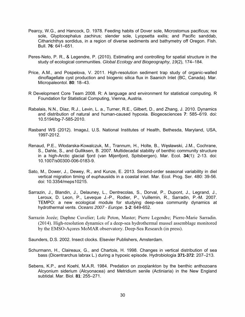
Tempo-mini and image acquisition

TEMPO-mini is a custom-designed instrument package created through a collaboration

between Ifremer‘s scientists and engineers for real-time monitoring of deep-sea benthic

communities and their habitats (Auffret et al. 2010). The TEMPO-mini ecological module is built

around a compact polyethylene structure assembled by titanium rods and bolts to save weight

and prevent corrosion during long-term deployments. TEMPO-mini uses a 2 megapixel high

resolution Axis 223M network camera integrated in a titanium housing, along with 4 x 20W LED

projectors. The package is also equipped with an Aanderaa optode for in situ oxygen

measurements, and a temperature probe.

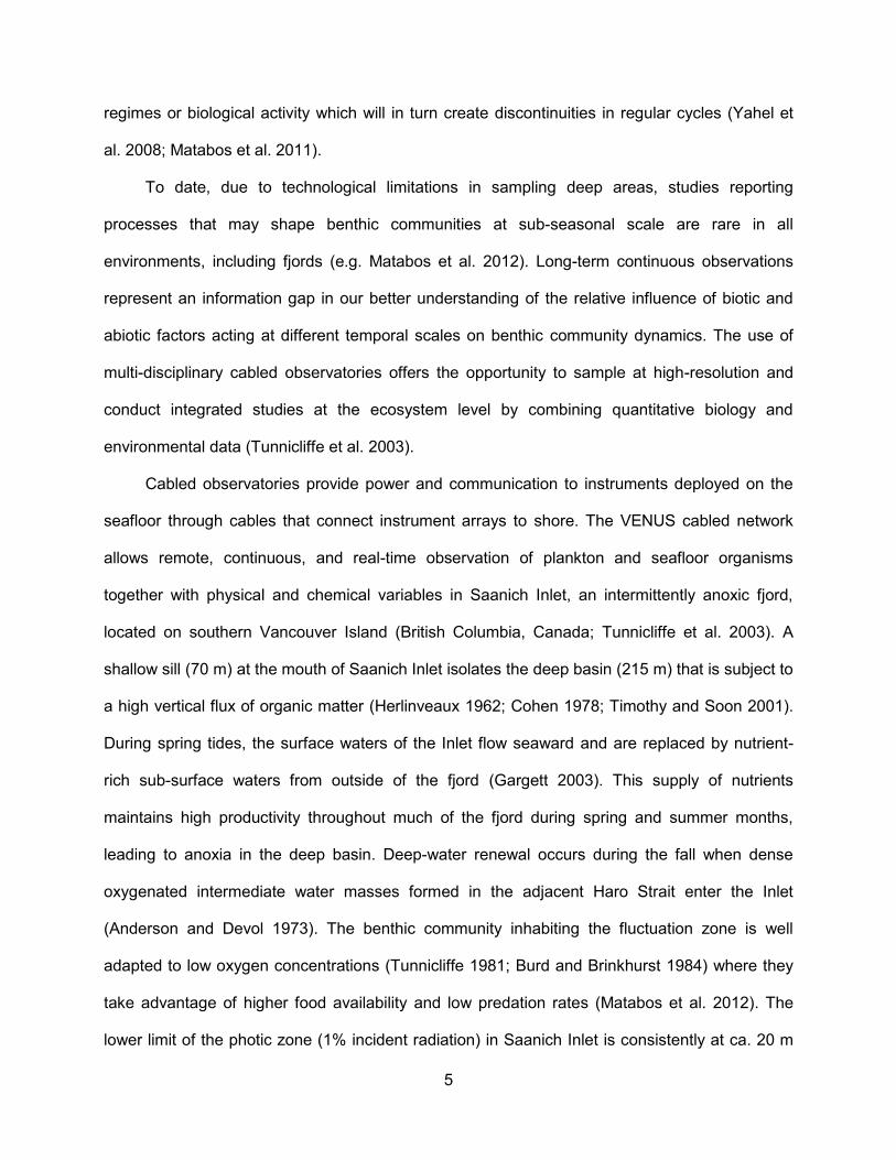
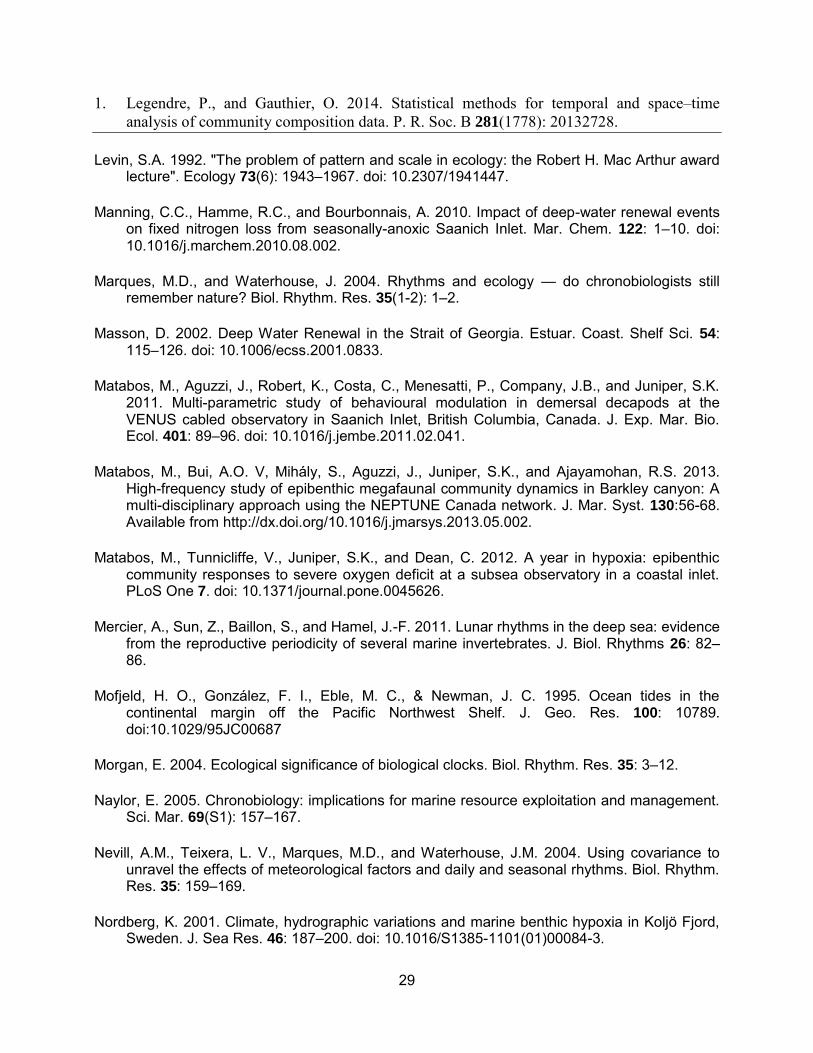
TEMPO-mini was deployed on a NEPTUNE Canada junction box at 97 m depth in Saanich

Inlet using the ship crane (Figure 1). On the bottom, the Remotely Operated Vehicle (ROV)

ROPOS connected the module to the VENUS network using its mechanical arm. The

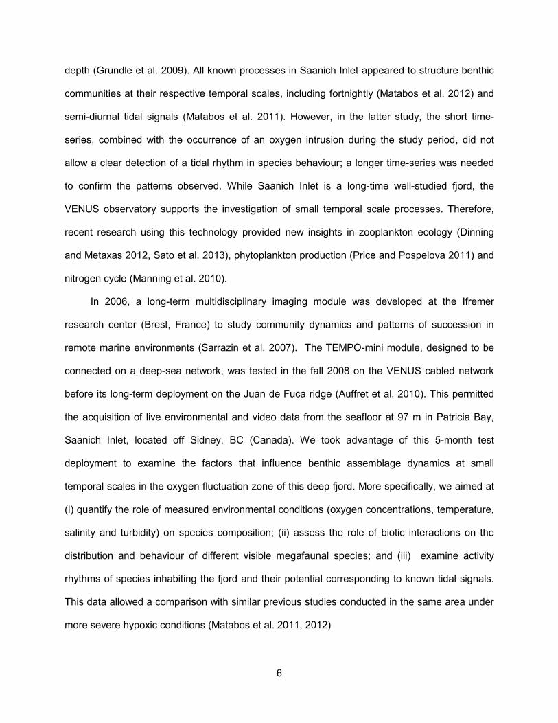
deployment occurred late September 2008 and the recovery early February 2009. The camera

was located at 60.5 cm above the bottom, in a 45° angle (Figure 2) and acquired 3 minutes of

video every half hour between October 28th 2008 and February 2nd 2009. However, due to

technical issues, no video imagery was acquired from September 28 to October 29, 2008,

generating a big gap at the beginning of the time-series. In addition, loss of power in LEDs and

biofouling issues resulted in poor visibility, and video images acquired in January and February

2009 were not usable. As a result, the sequences analysed only covered a 2 month period,

between October 30th and December 31st 2008.

Biological data extraction from video imagery

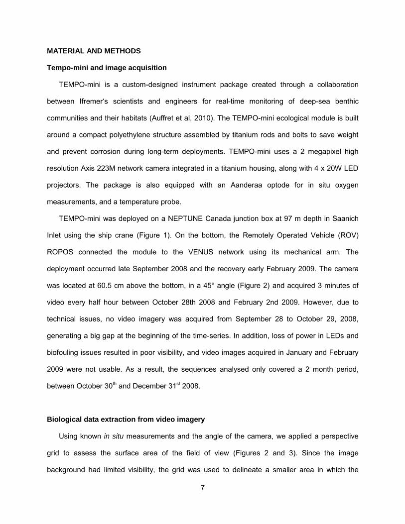
Using known in situ measurements and the angle of the camera, we applied a perspective

grid to assess the surface area of the field of view (Figures 2 and 3). Since the image

background had limited visibility, the grid was used to delineate a smaller area in which the

8

biological data were extracted in order to maintain consistency among images and limit errors.

Due to the huge amount of images generated, analyses include only one clip per hour, totalizing

24 clips of 3 minutes per day (half of the images). This subsampling provided enough high

frequency data acquisition to detect a potential semidiurnal rhythm. Animals were identified to

the lowest possible taxonomy level and counted using Image J 1.44 open source software

(Rasband, 2012).

Every hour, qualitative and semi-quantitative information were extracted from video clips

(Table 1). Organisms were analysed using two strategies depending on their mobility: mobile

species were characterized by density variations whereas the activity rhythm of sessile species

was recorded. It included length variations of anemone stalks (Figure 3) and tentacle orientation,

zooplankton density index and species presence/absence. The abundance of organisms was

extracted at the 30th second of the clip, 25 seconds after the lighting starts in order to minimise

its influence on the observations (Table 1). Individuals of each species observed in the studied

area were counted and species abundance data were converted to densities of individuals per

m2 by dividing the total number of individuals by the total surface area of 1.02 m2. The nutritional

behaviour of the anomurid squat lobster Munida quadrispina and species interactions were also

reported. All other relevant information regarding to behaviour or visible environmental

conditions was also documented (Table 1). The full data set analysed included 1381 video

sequences totalizing 69 hours and 30 minutes of imagery.

Environmental conditions

All environmental variables, i.e. dissolved oxygen concentrations, temperature, salinity and

turbidity, were obtained from the VENUS Instrument Platform (VIP). The VIP was located at 97.4

m depth and 75 m from TEMPO-mini (Figure 1).We therefore considered that the conditions

recorded at the VIP were representative of those experienced by the fauna observed by the

Tempo-mini module. For comparisons between environmental variables and observed changes

9

in megafaunal species, we computed the hourly average of each environmental variable using

data measured half an hour before and half an hour after the biological observations, to account

for the distance between the camera and sensors.

Uni- and bivariate analysis

Species association - In order to detect possible association among species, the kendall tau

rank correlation coefficient was computed for each pair of species using the cor.test function in

R.

Identification of significant periodicities -Periodicities in environmental data, species activity and

behaviour were screened using periodograms. A Whittaker-Robinson periodogram was used to

screen periodicities in quantitative data, i.e. species densities and environmental parameters,

and their statistical significances was tested by a permutation procedure (Legendre and

Legendre 2012). For the qualitative data, such as anemone lengths, tentacle orientation,

nutrition modes and biotic interactions, the contingency periodogram was selected (Legendre et

al. 1981) . This type of periodogram is based on a Buys-Ballot contingency table where each row

is the state (i.e. index value or 0/1 for presence-absence data) of the variable while in the

columns is reported the number of times an observation occurs in a given period (Legendre et

al. 1981).

Multivariate analyses

In analysis of community ecology, while Euclidean distance is inappropriate for ordination of

species abundance data with many zeros, the Hellinger distance is a measure recommended for

this type of data (Legendre and Legendre 2012). A Hellinger transformation was thus applied to

species density data prior to multivariate analyses. The transformation consists in taking the

square root of the relative abundance of each species at a given observation date. After this

10

transformation, analysis based on Euclidean distance like canonical redundancy analysis (RDA)

preserve the Hellinger distance among sites (Legendre and Gallagher 2001). The RDA, used to

assess the relation between species and environmental data, combines aspects of ordination

and regression and uses a permutation procedure to test the significance of the explained

variation (Legendre and Legendre 2012). All multivariate analyses were performed on

normalized (i.e. centred and scaled) environmental data. Calculations were performed through R

language functions (R Core Development Team 2013).

Identification of temporal breaks - First, putative temporal breaks were identified using a

multivariate regression tree (MRT) (De‘ath 2002) computed on two different datasets: (1) the

species density data, (2) and the environmental data matrix. This method defines groups of

dates that are similar in faunal composition/environmental conditions while temporally adjacent.

The MRT is a partitioning method of the multivariate response data table (i.e. species density

data or environmental matrix) constrained along the axis of a single explanatory variable, here

the time, to generate temporal consistent groups of observations. The tree structure is generated

by successively partitioning the whole dataset into mutually exclusive groups, and each split is

chosen to maximize the R² (or among sum-of-squares). The tree with the lowest cross-validation

error is chosen as the best predictive tree. At the end of the procedure, each leaf of the tree is

characterized by the number of observations and the value of the explanatory or constraining

variable (here time) defining each split (or node). The tree was computed using the ‗mvpart‘

library (De‘ath 2002) in the R statistical language.

Species assemblages temporal variability and influence of the environment- Prior to analysis,

multispecies data was checked for a linear trend and temporal structure of the faunal

assemblagewas investigated on residual data after detrending species density data. Data was

detrended using a RDA and all axes were kept (full model used). The temporal distribution of

11

species densities was then quantitatively described using distance-based Moran‘s Eigenvectors

Maps (dbMEMs; Borcard and Legendre 2002; Peres-Neto and Legendre 2010) on quantitative

data only. This method, more commonly used in spatial analysis of ecological studies, has been

successfully applied to time-series data for the detection and quantification of temporal variability

over a wide range of scales detectable by the sampling design (Angeler et al. 2009; Legendre

and Gauthier, 2014). We applied this technique to our time series to identify temporal variability

in species composition and densities of the studied assemblage. In this case, the method used

time coordinates of the sampling dates to build a matrix of Euclidean distances among

observation dates. This matrix was then truncated at a user defined threshold to only retain the

distance between neighbouring dates. In order to detect features smaller than the widest gap (54

hours), three observation dates were added to the time data vector, leaving a gap of 19 hours,

used as our truncation value (Borcard et al. 2004). A principal coordinate analysis (PCoA) on the

truncated distance matrix was computed and only the positive dbMEMs variables were kept.

Negative PCNMs describe negative correlations between neighbouring observations, in our case

two consecutive hours and are thus hard to relate to known natural processes or variability. After

the PCoA, the supplementary observation dates were removed from the dbMEMs matrix. This

generates a loss of orthogonality among the principal coordinates but the effect is negligible if

the number of added objects is small - in our case 3 out of 1381 observations (Borcard et al.

2004). The resulting principal coordinates (dbMEMs eigenfunctions) were irregular sinusoids

describing all the temporal scales that could be observed in the sampling design. The dbMEMs

variables were generated using the PCNM function implemented in the ‗PCNM‘ package (R

development Core Team 2013). Those dbMEMs variables were then used in a canonical

redundancy analysis (RDA), implemented in the ‗vegan‘ package (R Development Core Team

2013), to explain the variation in faunal assemblage structure (response variables) among

observation dates.

12

Significant dbMEMs functions were identified by a forward selection procedure (Dray et al.

2006) implemented in the ‗packfor‘ package (R development Core Team 2013). This procedure

uses the results of a permutation test (999 random permutations) to test the significance of the

explanatory variables (dbMEMs functions) successively entering the model and stops when

either the p-value of a newly included variable is higher than an alpha threshold of 0.05, or the

contribution (adjusted R2) of newly included variable is lower than a threshold equal to the

adjusted R2 value from the initial RDA. The significant dbMEMs functions were then plotted and

grouped into sub-models. The threshold for sub-models was defined according to known

environmental signals (e.g. tides) and processes, or when MEMs become non-significant

creating a large gap between groups of significant ones. Different thresholds were used to test

for the robustness of our choice and results remained unchanged. RDAs were used to test the

significance of each sub-model (i.e. time scale) on the biological matrix, followed by canonical

analyses of variance (ANOVAs) to test the significance of each RDA axis. The temporal sub-

models obtained were submitted to RDAs with environmental data to determine the explanatory

variables related to the species density data at each scale.

Relationships between zooplankton relative abundance, anemones‘ orientation and stalk‘s

length, squat lobster behaviour and environmental parameters were also investigated using

canonical redundancy analyses (RDA) as described above.

RESULTS

Environmental characterization

Dissolved oxygen (DO) concentration was low at the beginning of the study period

between October 28 and November 7, ranging between 0.12 and 0.70 ml/l. A first intrusion of

DO was recorded on November 8, 2008, with oxygen concentrations reaching 1.53 ml/l on

November 12, 2008 (Figure 4). A second, more important intrusion of DO occurred on

December 28th probably when a mass of cold, fresher water entering the mouth of Saanich Inlet

13

replaced the warmer, saltier, oxygen-depleted water (Figure 4) with hourly average DO

concentrations reaching 2.3 ml/l on December 31th, 2008. These oxygen intrusions were not

accompanied by changes in density. DO concentrations were highly variable at hourly scales,

especially during the intrusion events. Temperature and salinity varied little at the beginning of

the study period with values around 9.26°C (± 0.02 °C) and 31.12 PSU (± 0.05 PSU)

respectively. During the December 30th intrusion event, temperature reached a minimum of

8.34°C the next day and displayed a high hourly variability.

Transmission data translate the amount of turbidity in the study area, with 100% for no

turbidity and 0% when there is no light transmission, representing high turbidity. Values varied

between 45.7% and 70.9% over the study period, with a mean value of 64.6%. The 15 and 16 of

December were characterized by the highest turbidity levels (Figure 4).

Tides on this coast are mixed-semidiurnal with spring-neap amplitude variations (Mofjeld

et al. 1995). Periodograms performed on the raw hourly average data only detected periodicities

from 15 to 17 days in dissolved oxygen data (p < 0.05). After detrending the data, periodograms

highlighted a 15/17 days fortnightly periodicity for both DO concentrations and transmission rate,

and, for salinity, periodicities of 24 hours - in relation to the solar or lunar diurnal cycle - and 4/5,

8/9, 11, 13 and 16 days (Figure 5).

Species distribution patterns

Eight taxonomic groups (from species to family) and 8376 individuals were counted over

the entire period. The main mobile species encountered were the anomurid squat lobster

Munida quadrispina and pleuronectid flatfish mainly represented by the slender sole Lyopsetta

exilis (other flatfish occasionally present were the Pacific dover sole Microstomus pacificus, and

the English sole Parophrys vetulus). Other fish species were occasionally present in the field of

view including the bluebarred prickleback Plectobranchus evides, the blacktip poacher

Xeneretmus latifrons, a zoarcidae eelpout and a toadfish species. Sessile taxa were represented

14

by Suberitidae sponges and Metridium farcimen anemones. An unidentified nudibranch species,

comb jellies/ctenophores and the hyppolytidae shrimp Spirontocaris sica were also occasionally

seen. All species displayed high daily fluctuations in abundances (Figure 6). The squat lobster

Munida quadrispina was the most abundant species, with raw densities varying from 0 to 16

ind./m2 throughout the 2-month period, and occurred in higher number during December. Flatfish

density was higher early November at the beginning of the observation period. Other species

usually displayed low abundances (<2 ind./m2; Figure 6). Few individuals of toadfish were

observed between November 24th and 29th.

Species associations are presented in Table 2. Densities of the squat lobster M.

quadrispina were significantly negatively correlated with those of the flatfish, blacktip poacher

and toadfish, and positively correlated with those of the zoarcidae eelpout and bluebarred

prickleback (Kendall tau correlation coefficients, p < 0.05). Negative relationships were also

detected between flatfish densities and, those of the shrimp, eelpouts and toadfish; and between

toadfish densities and, those of eelpouts and shrimp. Significant positive relationships were

observed between densities of the toadfish and poachers, as well as between those of eelpouts

and shrimp.

Activity Rhythms

A wide range of rhythmicity characterized the different species observed in this study.

Only squat lobsters showed no significant periodicity (results not shown). Flatfish exhibited a

periodicity at 6 days and 14.5 days corresponding to the fortnightly spring/neap tide lunar cycle

(Figure 7). The eelpout displayed the same pattern with a periodicity at 1.5 days and ca. 12

days. The toadfish had only one significant periodicity at 19 days. The periodogram performed

on the prickleback revealed a 12 hours periodicity and the corresponding harmonics in relation

to the semi-diurnal tidal lunar cycle, as well as a significant rhythmicity at ca. 10, 13, 15 and 16

days. Finally the periodograms performed on poachers and shrimp were similar (Figure 7:

15

poachers) with a periodicity detected at 2.5 days and its harmonics at ca. 5, 10, 12 and 17.5

days. Poachers displayed an additional fortnightly periodicity of 15 days.

The orientation of the anemones‘ tentacles did not display any periodicity, and no rhythm

was detected in the M. quadrispina nutrition or biotic interactions. On the other hand, a ca. 4 and

8 day periodicities were highlighted in the stalk lengths of the two anemones (Figure 7).

Species assemblage dynamics: relationships between biological data and environment

The multivariate regression tree computed on environmental variables accounted for

55% of the total variance (Figure 8A). The first split explained 18.2% of the variance and

separated observations made ‗prior‘ and ‗after‘ the second big oxygen intrusion event recorded

on December 28th. Prior to that date, the second split correspond to the first oxygen intrusion

event on November 11th. The tree computed on species densities along the temporal axis

explained 23.5% of the total variance in species data and highlighted 4 main groups (Figure 8B).

The first split (21.6% of the variance) separated observations made ‗before‘ and ‗after‘

November 24th at 11:30. The secondary splits only explained 1.9% of the variance and

separated observations made ‗before‘ and ‗after‘ November 16th at 7:30 on one side and

December 4th at 9:30 on the other side. Observations made between November 24th and

December 4th were characterized by the presence of toadfish.

The set of environmental variables considered in this study only accounted for 7.71% of

the total variance in species density data. Even if a low proportion of variance is represented, the

two first axis of the RDA were significant at 0.05. The first axis of the redundancy analysis

explained 6.05% of the total variance and is strongly related with DO concentrations and light

transmission (Figure 9). The second axis explained 1.49% of the variance and was strongly

driven by salinity and transmission. In terms of species, toadfish contributed the most to the first

axis, related to higher DO concentrations while flatfish and squat lobsters contributed the most to

16

the second axis. A linear trend explaining 2.5% of the total variance in species density data was

detected.

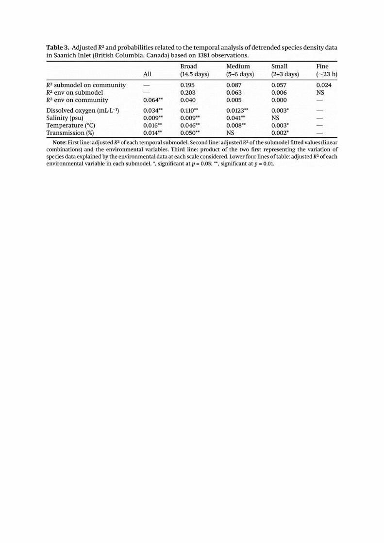
The dbMEM analysis lead to the identification of four scales of variation in the structure of

the benthic assemblage over the 2-month period: (i) broad (14.5 days), (ii) medium (4-6 days),

(iii) small (2-3 days) and (iv) fine (ca. 24 hours) (Table 3). The broad scale, corresponding to the

lunar fortnightly cycle, accounted for 19.5% of the total variance in the species density data and

was significantly related with all four water properties, with a higher correlation with DO

concentrations. Medium scale accounted for 8.7% of the total variance and was significantly

related to all variables but light transmission. Salinity contributed the most to that sub-model.

The small scale accounted for 5.7 % of the total variance and was also significantly related to all

variables but salinity. However, the contributions of the different water properties to this sub-

model were small. Finally, the fine scale accounted for only 2.4% of the total variance and was

not related to any of the environmental variables considered in this study. The 24 hours cycle

can be assimilated to the day/night diel cycle or the lunar diurnal tide.

DISCUSSION

Image acquisition with the ecological module Tempo-mini delivered high-resolution time-

series in the Saanich Inlet fjord (British Columbia, Canada) with hourly information on faunal

assemblage dynamics, including changes in species composition and species behavior. One

limitation in this study lays in the potential influence of the physical structure (Tempo-mini

module) and the artificial lighting on species behavior. The influence of lights on invertebrates is

unknown but this issue has recently been raised with the development of observatories and the

use of camera systems to study benthic faunal communities (Matabos et al. 2011, 2012). While

a study in the North Pacific showed no influence of the infrastructure on megafaunal

abundances (Vardaro et al. 2007), it is recognized that light can modify the behavior of certain

17

fish species (Krieger 1997; Widder et al. 2005; Doya et al. 2013, pers. observations). Here, the

structure and lights were constant over the entire study period and we are confident that the

changes we observed were mostly linked to external factors (Matabos et al. 2011, 2012). Finally,

the small field of view (1.02 m²) coupled with low species abundance might limit our ability to

detect activity patterns in mobile species like fish, and their extrapolations to larger scales should

therefore be considered cautiously.

Physiography, hydrography, including deep-water renewal, and weather are the most

important factors shaping fjord ecosystems habitats (Nordberg et al. 2001), and consequently

strongly influence the benthic community structure (Renaud et al. 2007, Blanchard et al. 2010,

Brewin et al. 2011). Limited circulation and isolation of deep basins in silled glacial fjords limit

nutrient exchanges and larval dispersal (Renaud et al. 2007). In addition, carbon fluxes are

generally low, resulting in low faunal abundances and biomasses (Blanchard et al. 2010).

Hence, water stratification, by controlling productivity and anoxia, would play a major role in

shaping fjord benthic communities (Timothy and Soon 2001, Blanchard et al. 2010, Brewin et al.

2011). In contrast, Saanich Inlet is one of the most productive fjords in the northern hemisphere

(Grundle et al. 2009), hence food is not a limitation for its benthic communities. In response to

this high productivity, hypoxia develops during summer and fall (Timothy and Soon 2001) and

the fauna, adapted to those low oxygen conditions, can survive for short periods of anoxia

(Tunnicliffe 1981; Matabos et al. 2012). Our results confirmed the role of oxygen on species

assemblage dynamics in Saanich Inlet, but also highlighted and confirmed the significant role of

lunar related fortnightly neap/spring tide forcing, and in a lesser extent the semi- diurnal tidal

signal, on environmental conditions, fish activity and consequently species assemblage

dynamics. Even though tides play an important role in fjord‘s hydrography (Gargett 2003),

chronobiology studies in other fjords are not yet available in the literature.

18

Environmental variations

Throughout almost the entire study period, dissolved oxygen concentrations were typical

of hypoxic conditions (i.e. 1.4 ml/l; Rabalais et al. 2010) and only reached oxic levels at the end

of December. Those conditions are typical of a normal year in Saanich Inlet where, during the

boreal fall, dense cold and oxygenated water enters over the inlet sill replacing deep anoxic

water (Anderson and Devol 1973, Gargett 2003). The origin of the water mass entering over the

inlet sill is a result of a complex interaction occurring in the neighboring Strait of Georgia, where

deep dense water originating from the continental shelf and entering through the Juan de Fuca

Strait mixes with the cold freshwater from the Fraser river discharge (Masson 2002). Those

intrusion events occur as pulses linked with tidal forcing. Following a deep intrusion, two neap

tides are necessary for the water to reach a density high enough to trigger a new flushing event

(Masson 2002). The occurrence of two different intrusion events, varying in intensity, observed

in this study probably result from this pulse mechanism. The second event had a stronger

signature with a visible decrease in temperature and salinity. However, while deep-water

renewals are known to be density-driven, the oxygen intrusions we observed were not

accompanied by significant changes in density (Figure 4). Indeed, at the VENUS node sensor,

oxygen changes appear to represent a bad proxy for deep renewal timing as some renewals

result in DO increase while others are characterized by DO decreases if less oxygenated water

from the depth is pushed upwards during the event (Manning et al. 2010). Therefore, water

flowing in front of the sensor is of different nature than the ‗non-mixed‘ dense oxygenated water

entering the sill.

Light transmission values are a proxy of water visibility and therefore of the concentration

of particles in the water. The visibility tended to decrease over the study period along with

salinity. High turbidity levels started November 27, going up until December 6, which correspond

to a visible decrease in transmission values, and what appeared to be higher current flows

19

around December 16 when the peak in turbidity was recorded. These changes in environmental

conditions were likely related to replacement of water masses following the pulses described

above rather than pure mixing processes. The Whittaker-Robinson periodograms did not detect

any significant periodicities in environmental variables except from 15 to17 days for the oxygen,

corresponding to the fortnightly tidal signal. The observed strong punctual pulses/events

probably masked more regular cycles in relation to known tidal (i.e. diurnal and fortnightly)

periodicities. Indeed, when computing the periodograms on detrended data, the 15/17 days

periodicity was also detected in salinity and transmission rate. These variations, close to the

lunar fortnightly cycle, could be explained by the role of spring tide mixing in nutrient renewal

that generates fortnightly phytoplankton blooms and strongly affects biogeochemical processes

(Gargett 2003, Grundle and Juniper 2011). In addition, salinity showed variations at lower

periods from diurnal lunar tide signal of 24 hours to 12.8 days.

Biological rhythms

Behavioural rhythms result from the entrainment (modulation) of animals‘ physiology by

predictable environmental fluctuations (Saunders 2002; Dunlap et al. 2004). While data on

rhythmic behavior for marine species inhabiting aphotic zones are scant, an emerging literature

on biological rhythms in deep areas devoid of light suggest the importance of tide- and lunar-

related rhythms in species activity (review in Aguzzi et al. 2011; Matabos et al. 2013; Doya et al.

2013, Cuvelier et al. in press) and reproduction (Mercier et al. 2011).

In this study, activity rhythms were highly variable among species. The two Metridium

farcimen anemones, visible in our images, showed 4/5 days and 8 days periodicities in their

stalk lengths. Those values do not correspond to any known environmental signal but the

presence of significant harmonics in the periodogram analyses suggests that they were not an

artefact. The observation of more individuals will help better characterize and explain the rhythm

observed. The detected signal might reflect a physiological endogenous rhythm linked to a

20

nutritional process. Nevertheless, the rhythm observed could not be related to periodicity in

zooplankton, the principal prey of M. farcimen (Sebens and Koehl 1984). Zooplankton densities

were only evaluated visually with a semi-quantitative index, and temporal variations patterns in

zooplankton densities from in situ sampling could have led to different results. A study

conducted over 2 years at the same location described the zooplankton vertical daily migration

variability using quantitative acoustic data and highlighted the influence of life history traits and

environmental cues in migration timing (Sato et al. 2013). The authors assumed that the

migrating layer was mainly composed of euphausids. In our study, the zooplankton was

composed of euphausids and copepods in proportions highly variable from day to day but no

diurnal pattern related to dial vertical migration (dvm) was observed. This suggests that the

TEMPO-mini camera does not constitute a good tool for estimating zooplankton migration

patterns at depth.

Four different patterns in activity rhythms were highlighted in mobile species. The flatfish

displayed a 6 day periodicity that did not coincide to any known cyclic signal, and a lunar related

fortnightly cycle at 14.5 days in relation to spring/neap tide forcing. Similarly, Matabos et al.

(2012) detected a fortnightly cycle (15 days) at 104 m depth in a benthic assemblage of Saanich

Inlet. During spring tide, increased tidal mixing outside of the fjord create a pressure gradient

with a seaward flow of surface water and an inward flow of nutrient-rich sub-surface waters

(Gargett 2003). Therefore, this nutrient injection in Saanich Inlet appears to support a fortnightly

cycle of phytoplankton blooms. Matabos et al. (2012) hypothesized that the community

responded to this tidal forcing through changes in abundance and activity of zooplankton, which

will mostly influence the planktivorous Lyopsetta exilis (Pearcy and Hancock 1978). Although the

‗flatfish‘ reported in this study is represented by different species, L. exilis appeared to be the

most dominant over the study period (pers. obs.). Interestingly, the only species displaying the

fortnight cycle were highly mobile fish which are more likely to promptly react to change in food

quality/availability. Several fish species, including the prickleback Plectobranchus evides and the

21

pelagic fish (results not shown), displayed a semi-diurnal cycle and a diel cycle. Since small-

scale significant periodicities had 12-hour harmonics, the observed pattern is more likely to be

tidally-driven rather than related to the day/night cycle. Indeed, a 12-hours rhythmicity along with

the corresponding harmonics suggest an influence of internal tidal waves which are known to

affect mixing processes and consequently physico-chemical conditions of deep basins‘ waters in

fjords (Inall and Rippeth 2002; Garrett 2003). Similarly, Wagner et al. (2007) showed the

occurrence of an endogenous clock in deep-sea fishes in relation with internal waves affecting

water flow variations. However, we were not able to determine if the observed signal was linked

to endogenous or exogenous rhythms in response to change in habitat condition. The shrimp

and poacher Xeneretmus latifrons exhibited similar periodicities in their abundances with a 2.5

days and harmonics at 5 and 9/10 days and a common periodicity at ~17 days. The 17-day

period coincided with the periodicity detected in dissolved oxygen concentration and might

explain the behavioral response observed in these two taxa. Finally, the squat lobster Munida

quadrispina did not display any rhythmicity supporting previous observations in the same area

(Matabos et al. 2011).

Species assemblage structure and environmental influence

Temporal variations in the epibenthic megafaunal community were assessed using

species densities. Over the 2 months, changes in environmental conditions only explained 7.7%

of variation in the structure of the observed assemblage while a regression performed along the

time explained 23.5% of that same variation. The multivariate regression tree compiled on

density data showed that the first split on November 24 explained 21.6% of the variance. The

most notable differences at this date mainly involved changes in the composition of the benthic

fish assemblage. Prior to November 24, this assemblage was dominated by the flatfish, while

after there was an increase in benthic fish diversity with the arrival of toadfish and poachers.

This change occurred 12 days after the first intrusion of dissolved oxygen in the area. In Saanich

22

Inlet, except for the flatfish Lyopsetta exilis, benthic fish are known to be less tolerant to severe

hypoxic conditions, migrating deeper in the basin only when conditions become milder (Matabos

et al. 2012). In this study, the prickleback Plectobranchus evides was present during the two-

month period. On the contrary, Matabos et al. (2012) reported that during severe hypoxic

conditions in another area of the fjord, only the highly tolerant Lyopsetta exilis, Munida

quadrispina and shrimp Spirontocaris sica were observed. One main difference was the

presence of sulfo-oxydizing bacteria Beggatioa spp. at the Matabos et al. (2012) site. These

bacteria develop at the oxic-anoxic interface where they oxidize reduced sulfides with molecular

oxygen (Jørgensen and Revsbech 1983a); they are known to rapidly migrate upwards, following

variations in oxygen concentrations in the sediments (Jørgensen and Revsbech 1983b). Their

presence is thus a proxy of diffusing sulfides from the subsurface anoxic sediment (Matabos et

al. 2012). In this study, no bacterial mat developed, suggesting that the surface sediment did not

reach anoxic conditions at the end of the summer. This probably explains the highest taxonomic

diversity observed. The second break on December 4 coincided with an increase in X. latifrons

and M. quadrispina densities, and more occurrences of the zoarcidae eelpout. These changes

were associated with a slight decrease in dissolved oxygen concentration until the next strong

intrusion event on December 28. Our results support the presence of an increased taxonomic

diversity at times where environmental conditions (mostly oxygen) become accessible for less

tolerant species.

The measured environmental variables explained 6.4% of the variance in species data,

while again, temporal variables (i.e. MEMs) accounted for a much higher proportion. Four

temporal submodels (i-iv) were defined from all significant MEMs to represent the temporal

structure of the epibenthic assemblage. The most important temporal component detected was

(i) the lunar fortnightly pattern, which was highly correlated with DO and in a lesser extent,

temperature. This pattern coincides with periodogram results obtained for both environmental

23

conditions and fish activity confirming the significant role of the lunar fortnightly cycle. Those

results support and reinforce observations presented by Matabos et al. (2012) who suggested

that the benthic communities responded to the neap/spring tidal forcing through changes in

physico-chemical parameters (mainly oxygen) and the abundance and activity of zooplankton

that feed on the enhanced phytoplankton production (see above; Gargett 2003).

The (ii) medium (5-6 days) and (iii) small (2-3 days) scales defined in the temporal model

of the epibenthic assemblage were also significantly correlated with environmental variables but

those correlations were weak. The medium scale coincided with periodicities detected in salinity

variations, which is the variable explaining most of the variance at that scale (Table 3), while the

small scale coincided with the shrimp and X. latifrons activity. The link with salinity does not

necessarily imply that there is a direct causal link to species activity, but the same underlying

process may have generated this common periodicity. While our study period only covered 2

months, it detected variations in faunal assemblage structure at the same scales as the one

identified in a full year study done at the same location (Matabos et al. 2012) suggesting that our

results are not specific to the boreal fall/winter season. A third oxygen intrusion occurred in

March 2009 leading to DO values ranging from 3 to 4 ml/l in spring and summer (VENUS data -

http://venus.uvic.ca/data/data-archive/). While scales of variations would probably remain

unchanged, we expect to find a higher species diversity in the summer months when oxygen

concentrations are higher (VENUS data, Matabos et al. 2012), diversity that would in turn affect

biotic interactions within the community.

Most of the variance, including patterns detected at smaller scales, was not explained by

the available environmental variables suggesting that other parameters might play an important

role in benthic community dynamics in Saanich Inlet. Knowing the low current values in the area

(averaging less than 5 cm/s; Yahel et al. 2008), it is unlikely that current variations explain the

biological patterns observed. On the other hand, biotic interactions like competition for food or

24

predation, or species life-history traits might explain part of the unexplained variation (Borcard et

al. 2004). The finest scale (iv) of the temporal model revealed the importance of the tidal cycle

(~24 hours) which probably reflects the role of species activity rhythms on assemblage

dynamics. However, in this analysis we only considered fluctuations in species abundances

(Aguzzi et al. 2012). Direct ethological observations could be useful to detect the origin of the

observed rhythms and to understand the behavioral mechanism underlying the fluctuations

observed. One solution would be to study the benthic species individually under constant

conditions to reveal intrinsic mechanism (endogenous) underlying the functioning of their

biological clock (Johnson et al. 2003, Chiesa et al. 2010). In addition, the full analysis of our

entire video dataset over a month could bring more insights on the mechanisms associated with

tidal related rhythms. However, the amount of time and human resources needed to process

such an amount of data is enormous, emphasizing the need for automated video processing

(reviewed in Aguzzi et al. 2012).

Conclusions

Video observation systems deployed on the seafloor provide access to information not

available before and represent great tools to detect and describe biological rhythms at depths

(Aguzzi et al. 2012; Doya et al. 2013, Sarrazin et al. in press, Cuvelier et al. in press) which are

essential to understand ecosystem functioning and dynamics (Marques and Waterhouse 2004;

Morgan 2004). While observations in the lab can bring important insights into the biology of

individual species, they cannot supplement observations in the field where the complexity of the

ecosystem is influenced by species interactions and the unpredictability of the environment

(Marques and Waterhouse 2004; Nevill et al. 2004). Thus, activity rhythms of animals can be

masked by factors like food availability (Fernandéz de Miguel and Aréchiga 1994), changes in

water masses (Matabos et al. 2013) and dissolved oxygen concentrations (Schurmann et al.

1998; Matabos et al. 2011). The need to statistically separate the effect of meteorological factors

25

and activity rhythms was recognized by Nevill et al. (2004). His method allows one to determine

how species activity co-vary with changing environmental conditions but is not applicable at the

system level when dealing with a multispecies assemblage in order to understand ecosystem

dynamics as whole. In this study the combination of in situ approach to observe species

behaviour and activity, combined to novel statistical approach like the distance-based Moran

Eingenvectors Maps (MEM) analysis which handles autocorrelation and temporal correlation,

demonstrated the ability of observatories to describe how species vary with changes in

environmental conditions at the multispecies level.

At larger scales, the main advantage of seafloor observatories lays in the ability to

conduct long-term survey and simultaneously measurements of multiple variables at a single

point. One interesting application is thus the detection of extreme events and monitoring of the

response of benthic communities (Gaines and Denny 1993). For example, benthic activity

rhythms in a submarine canyon were only detected when considering short time segments

corresponding to periods before and after storm events (Matabos et al. 2013). To date, there is

no standardized way of defining an event as their characterization is obviously dependent of the

type of habitats. Observatories represent new avenues to conduct science in the world‘s oceans.

They are just starting to provide preliminary direction and answers to determine thresholds of

environmental and faunal changes in different types of marine habitats. Understanding natural

changes of benthic communities is becoming urgent in an era where the oceans are rapidly

changing and in which the resources they contain are increasingly sought after.

Aknowledgements

The authors would like to thank the Ifremer engineer team (Ifremer/REM/RDT) for its dedicated

support in the design, maintenance and improvement of the TEMPO deep-sea modules over the

years. We would also like to thank P. Rodier for this help with the construction of the perspective

grid and drawing, J. Nephin for her help in video processing and J. Rose for his support in

26

technical issues. We would also like to thank the VENUS and ROV ROPOS teams for their

helpful collaboration on the field. Finally, we would like to thank two anonymous reviewers for

their helpful comments on a previous version of the manuscript. This work was part of M.

Matabos post-doctoral work funded by the Canadian Healthy Ocean Network.

References

Aguzzi, J., Bahamon, N., and Marotta, L. 2009. The influence of light availability and predatory behaviour of the decapod crustacean Nephrops norvegicus on the activity rhythms of continental margin prey decapods. Mar. Ecol. 30(3): 366–375.

Aguzzi, J., and Company, J.B. 2010. Chronobiology of deep-water decapod crustaceans on continental margins. Adv. Mar. Biol. 58: 155–225. Available from http://www.ncbi.nlm.nih.gov/pubmed/20959158.

Aguzzi, J., Company, J.B., Costa, C., Matabos, M., Azzurro, E., Manuel, A., Menesatti, P., Sarda, F., Canals, M., Delory, E., Cline, D.E., Favali, P., Juniper, S.K., Furushima, Y., Fujiwara, Y., Chiesa, J.J., Marotta, L., Bahamon, N., and Priede, I.G. 2012. Challenges to the assessment of benthic populations and biodiversity as a result of rhythmic behaviour: video solutions from cabled observatories. Oceanogr. Mar. Biol. 50: 233–284.

Aguzzi, J., Company, J.B., Costa, C., Menesatti, P., Garcia, J.A., Bahamon, N., Puig, P., and Sarda, F. 2011. Activity rhythms in the deep-sea: a chronobiological approach. Front. Biosci. 16: 131–150.

Anderson, J.J., and Devol, A.H. 1973. Deep water renewal in Saanich Inlet, an intermittently anoxic basin. Estuar. Coast. Mar. Sci. 1: 10. doi: 10.1016/0302-3524(73)90052-2.

Angeler, D.G., Viedma, O., and Moreno, J.M. 2009. Statistical performance and information content of time lag analysis and redundancy analysis in time series modeling. Ecology 90: 3245–3257. Available from http://www.ncbi.nlm.nih.gov/pubmed/19967879.

Auffret Y., Coail, J.-Y., Delauney, L., Legrand, J., Dupont, J., Dussud, L., Guyader, G., Ferrant, A., Barbot, S. Laes, A. (2009). Tempo-Mini: A Custom-designed instrument for real-time monitpring of hydrothermal vent ecosystems. Instru. Viewpoint. 8, 17.

Blanchard, A.L., Feder, H.M., and Hoberg, M.K. 2010. Temporal variability of benthic communities in an Alaskan glacial fjord, 1971-2007. Mar. Environ. Res. 69: 95–107. Available from http://dx.doi.org/10.1016/j.marenvres.2009.08.005.

Borcard, D., and Legendre, P. 2002. All-scale spatial analysis of ecological data by means of principal coordinates of neighbour matrices. Ecol. Modell. 153: 51–68. doi: 10.1016/S0304-3800(01)00501-4.

27

Borcard, D., Legendre, P., Avois-Jacquet, C., and Tuomisto, H. 2004. Dissecting the spatial structure of ecological data at multiple scales . Ecology 85: 1826–1832. Eco Soc America. doi: 10.1890/03-3111.

Brewin, P.E., Probert, P.K., and Barker, M.F. 2011. Relative influence of processes structuring fjord deep-water macrofaunal communities across multiple spatial scales. Mar. Ecol. Prog. Ser. 425: 175–191. doi: 10.3354/meps08994.

Burd, B.J., and Brinkhurst, R.O. 1984. The distribution of the galatheid crab Munida quadrispina (Benedict 1902) in relation to oxygen concentrations in British Columbia fjords. J. Exp. Mar. Bio. Ecol. 81: 1–20.

Chiesa, J.J., Aguzzi, J., Garcia, J.A., Sarda, F., De La Iglesia, H. 2010. Light intensitydetermines temporal niche switching of behvioural activity in deep water Nephrops novegicus (Crustacea: Decapoda). J. Biol. Rhythms 25: 277-287.

Cohen, Y. 1978. Consumption of Dissolved Nitrous-Oxide in an Anoxic Basin, Saanich Inlet, British-Columbia. Nature 272: 235–237.

Cuvelier, D., Legendre, P., Laes, A., Sarradin, P.-M., Sarrazin, J. Rhythms and community dynamics of a hydrothermal tubeworm assemblage at Main Endeavour Field – A multidisciplinarydeep-sea observatory study. PLoS ONE (in press)

De‘ath, G. 2002. Multivariate Regression Trees: A New Technique for Modeling Species-Environment Relationships. Ecology 83: 1105–1117. doi: 10.2307/3071917.

Dinning, K.M., and Metaxas, A. 2012. Patterns in the abundance of hyperbenthic zooplankton and colonization of marine benthic invertebrates on the seafloor of Saanich Inlet, a seasonally hypoxic fjord. Mar. Ecol. 34(1): 2-13;

Doya, C., Aguzzi, J., Pardo, M., Matabos, M., Company, J.B., Costa, C., Mihaly, S., and Canals, M. 2013. Diel behavioral rhythms in sablefish (Anoplopoma fimbria) and other benthic species, as recorded by the Deep-sea cabled observatories in Barkley canyon (NEPTUNE-Canada). J. Mar. Syst. 130/69-78. Available from http://dx.doi.org/10.1016/j.jmarsys.2013.04.003 [accessed 24 April 2013].

Dray, S., Legendre, P., and Peresneto, P. 2006. Spatial modelling: a comprehensive framework for principal coordinate analysis of neighbour matrices (PCNM). Ecol. Modell. 196: 483–493. doi: 10.1016/j.ecolmodel.2006.02.015.

Dunlap, J.C., Loros, J.J., and DeCursey, P. 2004. Chronobiology: Biological Timekeeping. Sinauer, Sunderland, Massachusets.

Fernandéz de Miguel, F., and Aréchiga, H. 1994. Circadian locomotor activity and its entrainment by food in the crayfish Procambarus clarkii. J. Exp. Biol. 190: 9–21.

Gaines, S., and Denny, M. 1993. The largest, smallest, highest, lowest, longest, and shortest: extremes in ecology. Ecology 74: 1677–1692. doi: 10.2307/1939926.

28

Gargett, A. 2003. Physical processes associated with high primary production in Saanich Inlet, British Columbia. Estuar. Coast. Shelf Sci. 56: 1141–1156. doi: 10.1016/S0272-7714(02)00319-0.

Garrett, C. 2003. Internal Tides and Ocean Mixing. Science (80-. ). 301: 1858–1859. American Association for the Advancement of Science. doi: 10.1126/science.1090002.

Glover, A.G., Gooday, A.J., Bailey, D.M., Billett, D.S.M., Chevaldonné, P., Colaço, A., Copley, J., Cuvelier, D., Desbruyères, D., Kalogeropoulou, V., Klages, M., Lampadariou, N., Lejeusne, C., Mestre, N.C., Paterson, G.L.J., Perez, T., Ruhl, H., Sarrazin, J., Soltwedel, T., Soto, E.H., Thatje, S., Tselepides, A., Van Gaever, S., and Vanreusel, A.. 2010. Temporal change in deep-sea benthic ecosystems: a review of the evidence from recent time-series studies. Adv. Mar. Biol. 58: 1–95. doi: 10.1016/B978-0-12-381015-1.00001-0.

Grundle, D.S., Timothy, D.A., and Varela, D.E. 2009. Variations of phytoplankton productivity and biomass over an annual cycle in Saanich Inlet, a British Columbia fjord. Cont. Shelf Res. 29: 2257–2269. Elsevier. doi: 10.1016/j.csr.2009.08.013.

Grundle, D.S., Juniper, S.K. 2011. Nitrification from the lower euphotic zone to the sub-oxic waters of a highly productive British Columbia fjord. Marine Chemistry 123: 173-181.

Herlinveaux, R.H. 1962. Oceanography of Saanich Inlet in Vancouver Island British Columbia. J. Fish. Res. board Canada 19: 1–37.

Inall, M., and Rippeth, T.P. 2002. Dissipation of tidal energy and associated mixing in a wide fjord. Environ. fluid Mech. 2: 219–240.

Johnson, C.H., Elliott, J.A., and Foster, R. 2003. Entrainment of circadian programs. Chronobiol. Int. 20: 741–774. Available from http://eutils.ncbi.nlm.nih.gov/entrez/eutils/elink.fcgi?dbfrom=pubmed&id=14535352&retmode=ref&cmd=prlinks.

Jørgensen, B.B., and Revsbech, N.P. 1983a. Colorless Sulfur Bacteria, Beggiatoa spp. and Thiovulum spp., in O(2) and H(2)S Microgradients. Appl. Environ. Microbiol. 45: 1261–1270. Available from http://aem.asm.org/cgi/content/abstract/45/4/1261.

Krieger, K.J. 1997. Sablefish, Anoplopoma fimbria, observed from a manned submersible. In Biology and Management of sablefish, Anoplopoma fimbria. Edited by M. Saunders and M. Wilkens. U.S. Dep. Commer., NOAA Technical Reports NMFS 130. pp. 39–43.

Legendre, L., Fréchette, M., and Legendre, P. 1981. The contingency periodogram: a method of identifying rhythms in series of nonmetric ecological data. J. Ecol. 69: 965–979. Available from http://www.bio.umontreal.ca/legendre/reprints/J Ecol 69, 1981.pdf.

Legendre, P., and Gallagher, E. 2001. Ecologically meaningful transformations for ordination of species data. Oecologia 129: 271–280. Springer. doi: 10.1007/s004420100716.

Legendre, P., and Legendre, L. 2012. Numerical ecology. Third edition. Elsevier, Amsterdam.

29

1. Legendre, P., and Gauthier, O. 2014. Statistical methods for temporal and space–time analysis of community composition data. P. R. Soc. B 281(1778): 20132728.

Levin, S.A. 1992. "The problem of pattern and scale in ecology: the Robert H. Mac Arthur award lecture". Ecology 73(6): 1943–1967. doi: 10.2307/1941447.

Manning, C.C., Hamme, R.C., and Bourbonnais, A. 2010. Impact of deep-water renewal events on fixed nitrogen loss from seasonally-anoxic Saanich Inlet. Mar. Chem. 122: 1–10. doi: 10.1016/j.marchem.2010.08.002.

Marques, M.D., and Waterhouse, J. 2004. Rhythms and ecology — do chronobiologists still remember nature? Biol. Rhythm. Res. 35(1-2): 1–2.

Masson, D. 2002. Deep Water Renewal in the Strait of Georgia. Estuar. Coast. Shelf Sci. 54: 115–126. doi: 10.1006/ecss.2001.0833.

Matabos, M., Aguzzi, J., Robert, K., Costa, C., Menesatti, P., Company, J.B., and Juniper, S.K. 2011. Multi-parametric study of behavioural modulation in demersal decapods at the VENUS cabled observatory in Saanich Inlet, British Columbia, Canada. J. Exp. Mar. Bio. Ecol. 401: 89–96. doi: 10.1016/j.jembe.2011.02.041.

Matabos, M., Bui, A.O. V, Mihály, S., Aguzzi, J., Juniper, S.K., and Ajayamohan, R.S. 2013. High-frequency study of epibenthic megafaunal community dynamics in Barkley canyon: A multi-disciplinary approach using the NEPTUNE Canada network. J. Mar. Syst. 130:56-68. Available from http://dx.doi.org/10.1016/j.jmarsys.2013.05.002.

Matabos, M., Tunnicliffe, V., Juniper, S.K., and Dean, C. 2012. A year in hypoxia: epibenthic community responses to severe oxygen deficit at a subsea observatory in a coastal inlet. PLoS One 7. doi: 10.1371/journal.pone.0045626.

Mercier, A., Sun, Z., Baillon, S., and Hamel, J.-F. 2011. Lunar rhythms in the deep sea: evidence from the reproductive periodicity of several marine invertebrates. J. Biol. Rhythms 26: 82–86.

Mofjeld, H. O., González, F. I., Eble, M. C., & Newman, J. C. 1995. Ocean tides in the continental margin off the Pacific Northwest Shelf. J. Geo. Res. 100: 10789. doi:10.1029/95JC00687

Morgan, E. 2004. Ecological significance of biological clocks. Biol. Rhythm. Res. 35: 3–12.

Naylor, E. 2005. Chronobiology: implications for marine resource exploitation and management. Sci. Mar. 69(S1): 157–167.

Nevill, A.M., Teixera, L. V., Marques, M.D., and Waterhouse, J.M. 2004. Using covariance to unravel the effects of meteorological factors and daily and seasonal rhythms. Biol. Rhythm. Res. 35: 159–169.

Nordberg, K. 2001. Climate, hydrographic variations and marine benthic hypoxia in Koljö Fjord, Sweden. J. Sea Res. 46: 187–200. doi: 10.1016/S1385-1101(01)00084-3.

30

Pearcy, W.G., and Hancock, D. 1978. Feeding habits of Dover sole, Microstomus pacificus; rex sole, Glyptocephalus zachirus; slender sole, Lyopsetta exilis; and Pacific sanddab, Citharichthys sordidus, in a region of diverse sediments and bathymetry off Oregon. Fish. Bull. 76: 641–651.

Peres‐Neto, P. R., & Legendre, P. (2010). Estimating and controlling for spatial structure in the study of ecological communities. Global Ecology and Biogeography, 19(2), 174–184.

Price, A.M., and Pospelova, V. 2011. High-resolution sediment trap study of organic-walled dinoflagellate cyst production and biogenic silica flux in Saanich Inlet (BC, Canada). Mar. Micropaleontol. 80: 18–43.

R Development Core Team 2008. R: A language and environment for statistical computing. R Foundation for Statistical Computing, Vienna, Austria.

Rabalais, N.N., Díaz, R.J., Levin, L. a., Turner, R.E., Gilbert, D., and Zhang, J. 2010. Dynamics and distribution of natural and human-caused hypoxia. Biogeosciences 7: 585–619. doi: 10.5194/bg-7-585-2010.

Rasband WS (2012). ImageJ, U.S. National Institutes of Health, Bethesda, Maryland, USA, 1997-2012.

Renaud, P.E., Włodarska-Kowalczuk, M., Trannum, H., Holte, B., Węsławski, J.M., Cochrane, S., Dahle, S., and Gulliksen, B. 2007. Multidecadal stability of benthic community structure in a high-Arctic glacial fjord (van Mijenfjord, Spitsbergen). Mar. Ecol. 34(1): 2-13. doi: 10.1007/s00300-006-0183-9.

Sato, M., Dower, J., Dewey, R., and Kunze, E. 2013. Second-order seasonal variability in diel vertical migration timing of euphausiids in a coastal inlet. Mar. Ecol. Prog. Ser. 480: 39-56. doi: 10.3354/meps10215.

Sarrazin, J., Blandin, J., Delauney, L., Dentrecolas, S., Dorval, P., Dupont, J., Legrand, J., Leroux, D. Leon, P., Leveque J.-P., Rodier, P., Vuillemin, R., Sarradin, P.-M. 2007. TEMPO: a new ecological module for studying deep-sea community dynamics at hydrothermal vents. Oceans 2007 - Europe. 1-2: 649-652.

Sarrazin Jozée; Daphne Cuvelier; Loïc Peton, Master; Pierre Legendre; Pierre-Marie Sarradin. (2014). High-resolution dynamics of a deep-sea hydrothermal mussel assemblage monitored by the EMSO-Açores MoMAR observatory. Deep-Sea Research (in press).

Saunders, D.S. 2002. Insect clocks. Elsevier Publishers, Amsterdam.

Schurmann, H., Claireaux, G., and Chartois, H. 1998. Changes in vertical distribution of sea bass (Dicentrarchus labrax L.) during a hypoxic episode. Hydrobiologia 371-372: 207–213.

Sebens, K.P., and Koehl, M.A.R. 1984. Predation on zooplankton by the benthic anthozoans Alcyonium siderium (Alcyonacea) and Metridium senile (Actiniaria) in the New England subtidal. Mar. Biol. 81: 255–271.

31

Timothy, D.A., and Soon, M.Y.S. 2001. Primary production and deep-water oxygen content of two British Columbian fjords. Mar. Chem. 73: 37–51. doi: 10.1016/S0304-4203(00)00071-2.

Tunnicliffe, V. 1981. High species diversity and abundance of the epibenthic community in an oxygen-deficient basin. Nature 294: 354–356.

Tunnicliffe, V., Dewey, R., and Smith, D. 2003. Research plans for a mid-depth cabled seafloor observatory in Western Canada. Oceanography 16: 53–59.

Vardaro, M.F., Parmley, D., and Smith Jr., K.L. 2007. A study of possible ―reef effects‖ caused by a long-term time-lapse camera in the deep North Pacific. Deep Sea Res. Part I Oceanogr. Res. Pap. 54: 1231–1240. doi: 10.1016/j.dsr.2007.05.004.

Wagner, H.-J., Kemp, K., Mattheus, U., and Priede, I.G. 2007. Rhythms at the bottom of the deep sea: cyclic current flow changes and melatonin patterns in two species of demersal fish. Deep Sea Res. Part I Oceanogr. Res. Pap. 54: 1944–1956.

Widder, E.A., Robison, B.H., Reisenbichler, K.R., and Haddock, S.H.D. 2005. Using red light for in situ observations of deep-sea fishes. Deep Sea Res. Part I Oceanogr. Res. Pap. 52: 2077–2085. doi: 10.1016/j.dsr.2005.06.007.

Yahel, G., Yahel, R., Katz, T., Lazar, B., Herut, B., and Tunnicliffe, V. 2008. Fish activity: a major mechanism for sediment resuspension and organic matter remineralization in coastal marine sediments. Mar. Ecol. Prog. Ser. 372: 195–209.. doi: 10.3354/meps07688.

Figures

Fig. 1.Location of instruments on the VENUS cabled network in Saanich Inlet (British Columbia, Canada). (A) Map of Saanich Inlet (top) and its location on Vancouver Island along the west coast of Canada (bottom). (B) Location of instruments in Patricia Bay, Saanich Inlet. VIP, VENUS Instrument Platform; TM, TEMPO-mini; Camera, VENUS camera.

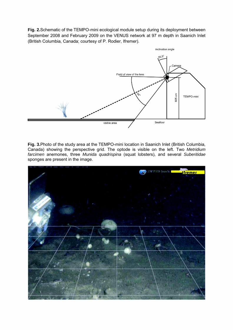
Fig. 2.Schematic of the TEMPO-mini ecological module setup during its deployment between September 2008 and February 2009 on the VENUS network at 97 m depth in Saanich Inlet (British Columbia, Canada; courtesy of P. Rodier, Ifremer).

Fig. 3.Photo of the study area at the TEMPO-mini location in Saanich Inlet (British Columbia, Canada) showing the perspective grid. The optode is visible on the left. Two Metridium farcimen anemones, three Munida quadrispina (squat lobsters), and several Suberitidae sponges are present in the image.

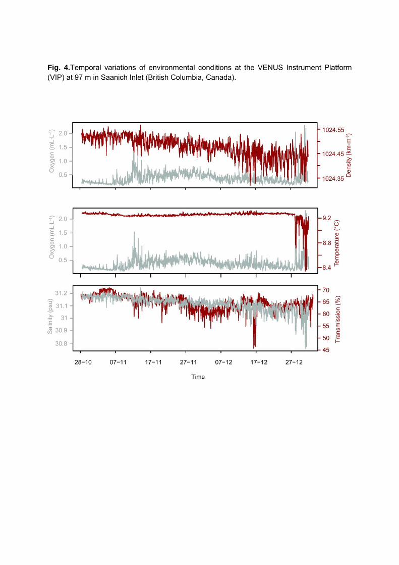
Fig. 4.Temporal variations of environmental conditions at the VENUS Instrument Platform (VIP) at 97 m in Saanich Inlet (British Columbia, Canada).

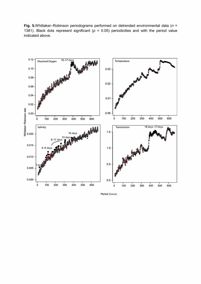
Fig. 5.Whittaker–Robinson periodograms performed on detrended environmental data (n = 1381). Black dots represent significant (p = 0.05) periodicities and with the period value indicated above.

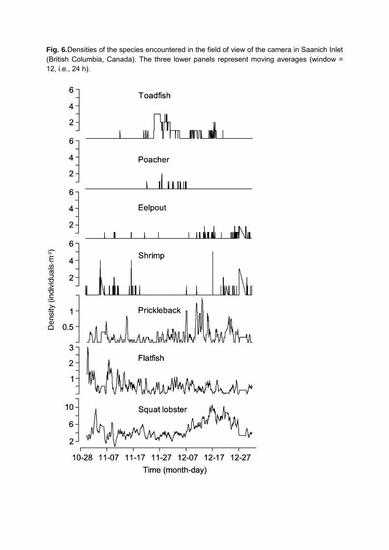
Fig. 6.Densities of the species encountered in the field of view of the camera in Saanich Inlet (British Columbia, Canada). The three lower panels represent moving averages (window = 12, i.e., 24 h).

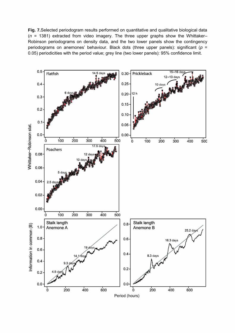
Fig. 7.Selected periodogram results performed on quantitative and qualitative biological data (n = 1381) extracted from video imagery. The three upper graphs show the Whittaker–Robinson periodograms on density data, and the two lower panels show the contingency periodograms on anemones’ behaviour. Black dots (three upper panels): significant (p = 0.05) periodicities with the period value; grey line (two lower panels): 95% confidence limit.

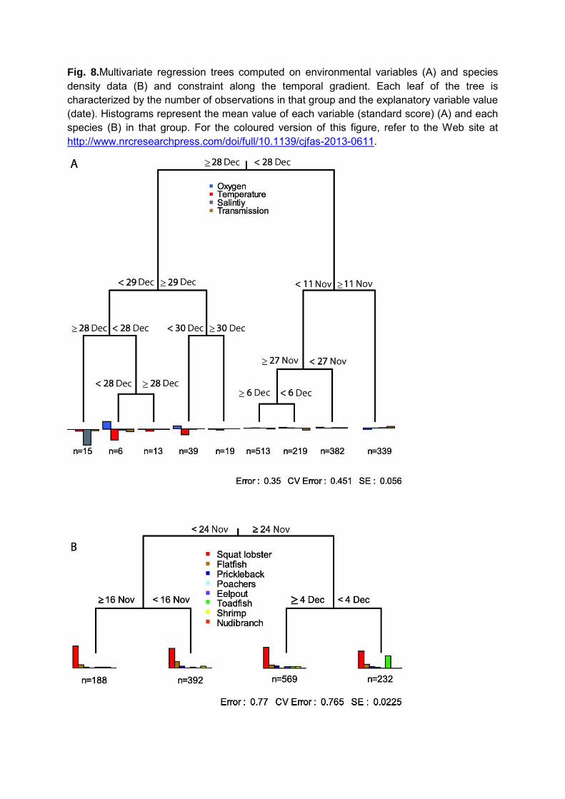
Fig. 8.Multivariate regression trees computed on environmental variables (A) and species density data (B) and constraint along the temporal gradient. Each leaf of the tree is characterized by the number of observations in that group and the explanatory variable value (date). Histograms represent the mean value of each variable (standard score) (A) and each species (B) in that group. For the coloured version of this figure, refer to the Web site at http://www.nrcresearchpress.com/doi/full/10.1139/cjfas-2013-0611.

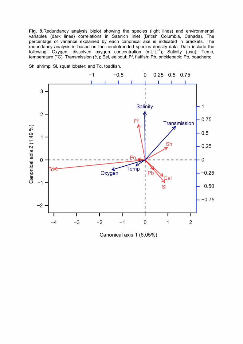
Fig. 9.Redundancy analysis biplot showing the species (light lines) and environmental variables (dark lines) correlations in Saanich Inlet (British Columbia, Canada). The percentage of variance explained by each canonical axe is indicated in brackets. The redundancy analysis is based on the nondetrended species density data. Data include the following: Oxygen, dissolved oxygen concentration (mL·L−1); Salinity (psu); Temp, temperature (°C); Transmission (%); Eel, eelpout; Ff, flatfish; Pb, prickleback; Po, poachers;

Sh, shrimp; Sl, squat lobster; and Td, toadfish.

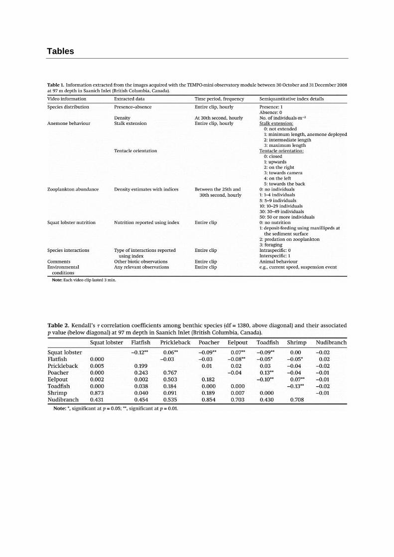
Tables