Icarus 234 (2014) 109–131

Contents lists available at ScienceDirect

Icarus

journal homepage: www.elsevier .com/locate / icarus

The variability of crater identification among expert and communitycrater analysts

http://dx.doi.org/10.1016/j.icarus.2014.02.0220019-1035/� 2014 Elsevier Inc. All rights reserved.

⇑ Corresponding author.E-mail address: stuart.robbins@colorado.edu (S.J. Robbins).

Stuart J. Robbins a,⇑, Irene Antonenko b,c, Michelle R. Kirchoff d, Clark R. Chapman d, Caleb I. Fassett e,Robert R. Herrick f, Kelsi Singer g, Michael Zanetti g, Cory Lehan h, Di Huang h, Pamela L. Gay h

a Laboratory for Atmospheric and Space Physics, University of Colorado at Boulder, 3665 Discovery Dr., Boulder, CO 80309, United Statesb Planetary Institute of Toronto, 197 Fairview Ave., Toronto, ON M6P 3A6, Canadac University of Western Ontario, 1151 Richmond Street N., London, ON N6A 5B7, Canadad Southwest Research Institute, 1050 Walnut Street, Suite 300, Boulder, CO 80302, United Statese Department of Astronomy, Mount Holyoke College, 50 College Street, South Hadley, MA 01075, United Statesf Geophysical Institute, University of Alaska Fairbanks, Fairbanks, AK 99775-7320, United Statesg Department of Earth and Planetary Sciences, McDonnell Center for the Space Sciences, Washington University in St. Louis, 1 Brookings Dr., Saint Louis, MO 63130, United Statesh The Center for STEM Research, Education, and Outreach at Southern Illinois University, Edwardsville, Edwardsville, IL 62025, United States

a r t i c l e i n f o a b s t r a c t

Article history:Received 15 June 2013Revised 20 February 2014Accepted 23 February 2014Available online 4 March 2014

Keywords:CrateringImpact processesMoonMoon, surface

The identification of impact craters on planetary surfaces provides important information about theirgeological history. Most studies have relied on individual analysts who map and identify craters andinterpret crater statistics. However, little work has been done to determine how the counts vary as afunction of technique, terrain, or between researchers. Furthermore, several novel internet-based pro-jects ask volunteers with little to no training to identify craters, and it was unclear how their results com-pare against the typical professional researcher. To better understand the variation among experts and tocompare with volunteers, eight professional researchers have identified impact features in two separateregions of the Moon. Small craters (diameters ranging from 10 m to 500 m) were measured on a lunarmare region and larger craters (100s m to a few km in diameter) were measured on both lunar highlandsand maria. Volunteer data were collected for the small craters on the mare. Our comparison shows thatthe level of agreement among experts depends on crater diameter, number of craters per diameter bin,and terrain type, with differences of up to �±45%. We also found artifacts near the minimum crater diam-eter that was studied. These results indicate that caution must be used in most cases when interpretingsmall variations in crater size–frequency distributions and for craters [10 pixels across. Because of thenatural variability found, projects that emphasize many people identifying craters on the same area andusing a consensus result are likely to yield the most consistent and robust information.

� 2014 Elsevier Inc. All rights reserved.

1. Introduction

Impact craters are among the most common and numerous fea-tures on planetary surfaces in the Solar System. They have beenused for decades in various studies, from understanding thedynamics of the Solar System to being a ‘‘poor man’s drill’’ by exca-vating through numerous rock layers. This research relies on a keyassumption: Impact craters can be reliably identified. Manyapplications, especially age estimates (McGill, 1977), also rely onmeasurements of crater diameter. It is generally assumed that bothidentification and measurement are trivial, but limited studies

have shown this to not always be true; variations in crateridentification and diameter measurement on the order of �10% be-tween individuals using the same measuring technique have beenfound (e.g., Gault, 1970; Greeley and Gault, 1970; Kirchoff et al.,2011; Hiesinger et al., 2012).

Gault (1970) had approximately 20 people identify 1.3 millioncraters using Zeiss particle counters (this device allows the opera-tor to match a pre-set circle size or ‘‘size class’’ of projected lightonto a photograph, prick a hole through the photograph at the cra-ter center, and the diameter is automatically registered on theinstrument’s display). He concluded, ‘‘‘Calibration’ and continuouscross-checks of each individual’s work indicate that crater countsby different persons generally agree and/or can be reported within±20%. . .’’ Greeley and Gault (1970) used the same technique anddata to further describe the dispersion among researchers.

110 S.J. Robbins et al. / Icarus 234 (2014) 109–131

Measurements were made by five individuals on a single imageand showed good agreement for small craters but dispersion inthe number of craters among the largest diameters (their Fig. 3).Greeley and Gault (1970) found less than ±20% deviation fromthe mean for counts of >100 craters in a given size class, ‘‘a valuethat probably represents an irreducible minimum deviation im-posed by the subjectivity of the counting.’’ This variation rose to±100% for counts with <4–5 craters in a given size class. Theauthors emphasized that a single individual may perform moreconsistent counts, but individual biases and differences from oneday to the next – indeed, one hour to the next – explain whymultiple individuals identifying craters on the same terrain arelikely to yield the most reliable results.

Kirchoff et al. (2011) provide a more recent comparison withthree researchers (two expert, one novice without crater countingexperience) from the same lab who used the same technique toidentify, measure, and, in this case, classify craters by preservationstate. They used Lunar Reconnaissance Orbiter Camera Wide-AngleCamera (LROC WAC) images of Mare Orientale. The two experi-enced analysts had counts that differed by 20–40% in a given diam-eter range, while the novice counter identified numerous featuresthat are probably not craters, differing from the other two by>100% over some diameter ranges. They also had significant varia-tion among the preservation states attributed to each crater, de-spite a relatively coarse four-point scale. This work showed thatdespite common thinking that crater counting is fairly easy andstraightforward, there is a learning curve and an individual’s cratercounts should be discarded during the learning process. It alsoshowed that even well defined crater morphologies may be diffi-cult to classify uniformly.

Hiesinger et al. (2012) also focused on lunar craters, in theircase using LROC Narrow-Angle Camera (NAC) images at approxi-mately 0.5 m/px. They were interested in reproducible results forbetter understanding the lunar cratering flux and performed a sin-gle test with two experienced researchers who used the same tech-nique on the same image. The Hiesinger et al. (2012) team foundan overall variation of only ±2% between their analysts, a disper-sion significantly less than previous work.

What this brief review indicates is that while there has beensome discussion in the literature about agreement between differ-ent researchers’ crater identifications, (a) there has been no thor-ough discussion on researcher variability, (b) no published studydiscusses the variability when using different techniques for crateridentification and measurement, (c) variation in crater morphologyhas not been discussed (e.g., sub-km craters appear substantiallydifferent at NAC pixel scales when compared with multi-km cratersat WAC pixels scales), and (d) expert results have not been exten-sively compared with how well untrained or minimally trained cra-ter counters do with the identification and measurement process.Given the proliferation of internet crowd-sourcing projects thatask laypeople to help in the data-gathering process, this last pointdetermines if the public can assist in crater counting and produceresults that are approximately as reliable as the experts.

For these reasons, the following work was undertaken. Eightresearchers, with six to fifty years of experience identifying craters,identified and measured the diameter (D) of craters on a segmentof a NAC image. This same region was also analyzed by volunteer‘‘citizen scientists’’ through CosmoQuest’s Moon Mappers (‘‘MM’’)project which facilitates volunteer identification and measurementof craters and other features that are being studied in a variety oflunar research projects (Robbins et al., 2012; http://cosmo-quest.org). In addition, the experts identified and measured craterson a WAC image that covers both lunar mare and highlands. Theexperts worked independently, with each researcher using theirown preferred technique (in total, seven different methods wereemployed).

These methods and the counting locations are discussed in Sec-tion 2 along with terminology, our display techniques, and statisti-cal tests in Section 2.4. Section 3 describes steps taken to ensurethat our analysis is based solely on how different people identifycraters, including how experts varied (Section 3.1), how well thevolunteers compared with experts (Sections 3.2 and 3.3), andhow our data reduction process may affect results (Sections 3.4and 3.5). Section 4 describes the overall crater populations foundin each image and the variation among experts and between ex-perts and volunteers. Section 5 moves from the population of cra-ters from Section 4 to how well experts and volunteers agreed onthe measurements of individual craters. Section 6 is an analysisof how crater detection depended on preservation state. Section 7describes artifacts that we found near the minimum crater diame-ter. Section 8 is a short discussion of likely reasons for differencesamong experts and between them and volunteers. Section 9 sum-marizes the work and discusses implications and conclusions.Appendix A provides additional details on each researcher’s tech-nique, Appendix B summarizes each researcher’s experience inthe field, and Appendix C more thoroughly discusses our datareduction methods.

2. Methodology

2.1. Images used

This work was motivated in part by the need to determine howuntrained ‘‘citizen scientists’’ compare with experts. The experts inthis study were asked to identify and measure craters in the sameLROC NAC image that has been most studied by MM volunteers:M146959973L (Fig. 1). A portion of this image has been viewedby every MM volunteer because it is used as a calibration imageto assess how well each individual performs. The image has a solarincidence angle of 77�, meaning that useful shadows are present toenhance local topography for better feature identification. It is alsoof general interest because it contains the Apollo 15 landing site.MM uses a 4107 � 6651-pixel sub-image of M146959973L that iscentered on the Falcon lander. The experts in this study were givena sub-image 33% of this size (Fig. 1), 4107 � 2218 pixels, to maxi-mize participation among busy scientists. This sub-image containson the order of 1000 craters D P 18 pixels (the limit of the MMinterface).

The second image in this study was an LROC WAC that encom-passes both mare and highland areas to allow comparison of expertcrater identification on the two main lunar terrain types. The1311 � 2802-pixel selected portion of WAC M119455712M coversthe southern margin of Mare Crisium and the neighboring rim/highlands to the south (Fig. 2). It has a solar incidence angle of59�, which is on the boundary of what is considered ideal for crateridentification (Wilcox et al., 2005; Ostrach et al., 2011; Robbinset al., 2012).

Each image was downloaded from the Planetary Data Systems(PDS), processed in the USGS’s Integrated Software for Imagers andSpectrometers (ISIS) via standard radiometric and geometric tech-niques, projected to a local Mercator projection, exported as PNGfiles, and distributed to each researcher. For several of the crateridentification and measurement techniques, GIS-ready files wererequired. To ensure uniformity, Robbins imported the images intoArcMap and exported the GIS-ready files, and he distributed themto the researchers, too.

2.2. Techniques and personnel

Each researcher employed one or more different interfaces andmethods, with Robbins using two interfaces and Antonenko using

Fig. 1. Left two panels are the full NAC areas analyzed in this study with markings overlaid. Top image shows expert markings, bottom shows volunteer data; both showcraters only D P 18 px. The expert markings are color coded to correspond with the colors in Fig. 7. White, thicker circles are results from the clustering algorithm (seeSection 2.3). On the right side, four example craters are shown in detail with expert markings and reduced craters (left column) and volunteer data and reduced craters (rightcolumn); the craters are in order of increasing modification/degradation with class 1 at the top and class 4 at the bottom (see Section 6 and Table 3). Captioned below eachpair is the number (N) of persons who marked that crater and the mean diameter (D) with standard deviation. Values in parentheses are relative standard deviations(standard deviation of diameter divided by mean diameter; standard deviation of position divided by mean diameter). (Print version shows individuals’ craters as dark, thincircles and cluster results as light, thick circles.) (For interpretation of the references to color in this figure legend, the reader is referred to the web version of this article.)

S.J. Robbins et al. / Icarus 234 (2014) 109–131 111

three to replicate their NAC crater counts; Antonenko used two forher WAC counts. The software and methods used are briefly de-scribed here and they are detailed in Appendix A. Tables A1 andA2 summarize the numbers of craters found, methods used, andimage manipulation applied by each researcher.

The most common software was ESRI’s ArcGIS suite, withAntonenko, Fassett, Herrick, Robbins, Singer, and Zanetti using it.However, four different methods were employed. Robbins used na-tive tools to trace crater rims and then his own software to auto-matically batch-fit circles to each traced rim. The otherresearchers used software extensions. Fassett and Zanetti used‘‘CraterTools’’ (Kneissl et al., 2011) which uses a three-point meth-od to determine a circle; Herrick also used this interface for hisWAC dataset. Antonenko and Herrick (the latter for NAC data only)used the USGS’s ‘‘Crater Helper Tools’’ which also applies a three-point circle identification technique (Nava, 2011). Singer usednative tools to draw a chord through the crater center, from rimto rim, and the spherical length is calculated using Jenness Enter-prise’s ‘‘Tools for Graphics and Shapes’’ (Jenness, 2011).

The second-most common software application for experts wasJMARS, produced and maintained by Arizona State University(http://jmars.asu.edu). This was used by Antonenko (secondinterface) and Kirchoff. JMARS has a built-in crater measurement

tool that has two options for determining the diameter:three-point circle fits (Kirchoff) and a re-sizeable circle tool(Antonenko).

The third interface, used only by Chapman, was the SmithsonianAstrophysical Observatory’s DS9 (not an acronym) visualizationsoftware with several add-on tools written by various researchers.For crater handling, the POINTS tool, developed at Cornell, was usedwhich requires researchers to identify an even number of pointsalong the crater rim. The researcher then enters a numerical craterpreservation state to complete the identification, and a circle (orellipse) is fit.

The fourth software was the Moon Mappers online interface,used by Antonenko (as her third interface), Robbins (as his secondinterface), and all lay volunteers; this software was only used forthe NAC image. To identify a crater, the user clicks on (or near)the crater center and drags outwards, dynamically displaying a cir-cle of that radius and center position. The circle is color-codedbased on size: red if the diameter is D < 18 px and green whenD P 18 px (red craters are considered too small for confident iden-tification by MM volunteers). When the user is satisfied that thedrawn circle matches the crater, they release the mouse. Greencraters are saved and displayed (red craters are discarded), butthey can still be moved, re-sized, and erased if desired. In MM,

Fig. 2. Left panel is the full WAC area analyzed in this study with markings overlaid (only D P 7 px craters are shown). The markings are color coded to correspond with thecolors in Fig. 7, and white, thicker circles are results from the clustering algorithm. White dashed lines indicate boundaries between highlands and mare units. Right columnfollows Fig. 1 except are for mare (left) and highlands (right) craters as opposed to expert and volunteer, with data below each being mare (first line) and highlands (secondline). (Print version shows individuals’ craters as dark, thin circles and cluster results as light, thick circles.) (For interpretation of the references to color in this figure legend,the reader is referred to the web version of this article.)

112 S.J. Robbins et al. / Icarus 234 (2014) 109–131

images are shown in 450 � 450 pixel sub-sections, but differentimages are at different ‘‘zoom’’ levels to allow crater identificationover a large range of diameters. The 18-px cutoff was chosen to (a)limit the number of craters volunteers need to identify on any sin-gle image (avoid user fatigue), (b) the approximate limit to whichlay persons can easily identify a crater (determined during devel-opment work at Southern Illinois University Edwardsville), (c) istwo pixels smaller than 20-px, which was our original buffer,due to technical limitations at the time, and (d) ensures craters

D J 10 m will be identified when using average-resolution NACimages.

All expert researchers involved in this project have at least sixyears experience identifying and measuring craters, and one(Chapman) has over fifty years experience in this work. In contrast,the MM volunteers have no stated experience, and though Robbinsand Antonenko both have marked a few craters for the MM projectand so contributed to the ‘‘volunteer’’ dataset, it is safe to estimatethat �1% of MM craters were marked by experts.

S.J. Robbins et al. / Icarus 234 (2014) 109–131 113

2.3. Cluster analysis to compare craters and create a reduced catalog

Before any analysis could be conducted, the various measure-ments had to be properly aligned and in the same units; we choseto perform all analyses in pixel space in order to be scale-indepen-dent (i.e., all units are pixels and we compare NAC and WAC diam-eter-dependent results in pixels as opposed to meters andkilometers). Robbins’, Chapman’s, and all MM-marked craters werealready in pixel space upon export from software. For all otherdata, crater diameters and locations were scaled linearly by thepixel scale (m px�1) output from ISIS. The NAC image was small en-ough and close enough to the equator that a non-linear transformwas unnecessary. Non-pixel-space crater locations and diametersfor the WAC image were corrected by cos(latitude) to convert topixel space after the initial linear scaling.

After these corrections were applied and all craters were in pix-el space (Fig. 1 (NAC) and Fig. 2 (WAC)), a clustering code was usedto separately group the expert and volunteer markings into ‘‘re-duced’’ crater catalogs for subsequent analysis. Most analyses pre-sented in the next section require such a reduced catalog todetermine how the markings varied for each crater.

We detail the development of the clustering code in AppendixC. In brief, the automated code was a modified two-dimensionalDBSCAN (Density-Based Spatial Clustering of Applications withNoise) developed by Ester et al. (1996). The original code requiresonly two a priori inputs: a ‘‘reachability’’ parameter and the mini-mum number of points in a group required to be considered a validcluster. Reachability is how cluster members are found, where apoint is considered ‘‘reachable’’ by another point if it is within acertain distance of it or other members of the cluster to which itmay belong.

The code was modified to incorporate a diameter-dependentscaling of distance and to include a second reachability parameterdependent solely on diameter. The former means that, for example,two 20-px-diameter craters 10 pixels away from each other wouldnot be considered reachable and hence members of different clus-ters, but two 200-px-diameter craters 10 pixels away would beconsidered the same feature. The latter means that if a craterwas reachable by another based on location, it also needed to bereachable based on diameter. This allows us to separate overlap-ping craters, i.e., a small crater superposed on a larger crater thatunder a normal two-dimensional DBSCAN code would be groupedtogether into one feature.

The input data were crater location {x, y} and diameter D inaddition to the confidence c. Confidence is a score from 0 to 1 usedto rate how well each MM volunteer performs versus an expert(Robbins) on calibration images, and it is used to calculateweighted means of the clustered craters. For experts, we setc = 1. The data output for each cluster of markings are: (a)weighted mean �x with sample standard deviation, dx; (b) weightedmean �y with standard deviation, dy; (c) weighted mean D withstandard deviation, dD; (d) number of points N in that cluster;and (e) weighted mean of the confidence for the craters that wentinto that cluster, �c.

2.4. Terminology, display techniques, and statistical tests

In this section, we detail the comparison of expert crater mark-ings and how those relate to volunteer results. After Section 3, un-less otherwise stated, all ‘‘catalog,’’ ‘‘reduced,’’ or ‘‘ensemble’’expert data are from the clustered results of all expert data (11 to-tal interface/expert combinations for NAC, 9 for WAC) where N P 5persons (NAC) or P4 persons (WAC) needed to find the crater for itto count; the data were clustered even if the diameters were smal-ler than a stated a priori cut-off (18 px for NAC), and the cut-off wasperformed on the post-clustered results. The volunteer data are the

output from the clustering code with N P 7 persons having identi-fied the crater, unless otherwise stated (images were viewed by12–26 people). All error bars on crater populations are based onPoisson counting statistics (N1/2 where N is the number of cratersfound) unless otherwise stated. All error bars on other analysesare based on Gaussian sample standard deviations (square-rootof the variance normalized by N) unless otherwise stated.

We present and analyze the crater measurements in bothcumulative and relative size–frequency distributions (CSFD andR-plot; Crater Analysis Techniques Working Group, 1979). TheCSFDs are shown as true cumulative counts without binning. Weuse the Kolmogorov–Smirnov (K–S) test, which determines if twomeasured distributions come from distinct distributions, to com-pare the identified craters’ CSFDs. This test finds the maximumvertical separation between the two curves for the full range ofx-values (we use crater diameter), normalized to a cumulativevalue of 1.0. This maximum is then compared with expected valuesto determine the probability (P-value) that the null hypothesis (thedistributions are the same) is rejected. We used a P-value of >0.05to accept the null hypothesis. A P-value of 60.05 is used to statethat two populations are likely different, and a P-value of 60.01is interpreted to reject the null hypothesis and state that theyare different; 0.05 is the most common value used in statisticsbut the smaller value was used because the K–S test does not takeerror bars into consideration.

3. Results: overall crater population: separating independentvariables before analysis

In this sub-section, we present a step-by-step analysis of thenumbers of craters found and how well they match with individualresearchers’ results. We do this across all combinations of individ-uals and interfaces to determine where – if at all – artifacts orbiases may arise that affect the later analyses.

3.1. How do the experts vary in their interfaces of choice?

One of the fundamental questions in this study is: What is thevariation among experts and what role does interface play in thisvariation? These are motivated by a desire for the ‘‘right answer’’about the number of craters on a given surface, and this has impli-cations regarding uncertainty for studies such as the modeled sur-face ages. The top portion of Table 1 provides a summary of thenumbers of craters found by each expert in the NAC data, listedby expert and interface, and separated into crater diametersD P 18, 20, 25, 30, 50, and 100 pixels. The next two portions of Ta-ble 1 show the mean, median, standard deviation, and relativestandard deviation ‘‘rR’’ (standard deviation divided by the mean)among the experts for these different diameters for all interfacesexcept MM and then with the expert data from MM included (datafrom MM is treated separately at first to show whether it can accu-rately replicate results from the other interfaces). Table 2 showsthe same information for the WAC image, separated into highlandsand mare units, with no MM data (since that interface was notused in the WAC study). These data are also shown in Fig. 3(NAC) and Fig. 4 (WAC) as a function of diameter.

NAC: The data indicate there is at least ±20% dispersion amongexperts in the number of craters found at any given diameter in theNAC data. In their interfaces of choice, the relative standard devia-tion (rR) is a minimum of 20.7% for D P 18 px craters and grows to31.5% for D P 100 px craters (Fig. 3). A hypothesis we test in Sec-tion 6 is whether this may be due to crater preservation state be-cause large, degraded craters are numerous in this region of theMoon and at this pixel scale. Alternatively, we might conclude thatexperts converge better when a region is dominated by numerous

Table 1Summary of the numbers of craters found in the NAC image larger than or equal to different pixel cut-offs by the different researchers in

the different interfaces. ‘‘Std. Dev.’’ are standard deviationsffiffiffiffiffiffiffiffiffiffiffiffiffiffiffiffiffiffiffiffiffiffiffiffiffiffiffiffiffiffiffiffiffiffiN�1 P ðxi � lÞ2

q� �and ‘‘Rel Std. Dev.’’ is the standard deviation normalized by

the mean l�1ffiffiffiffiffiffiffiffiffiffiffiffiffiffiffiffiffiffiffiffiffiffiffiffiffiffiffiffiffiffiffiffiffiffiN�1 P ðxi � lÞ2

q� �. Also shown are different methods of determining the ‘‘best’’ number of craters in the image. Boxed

values for ‘‘N P # people’’ correspond to the best matches with the mean, and the bolded row is the row used for all analyses in themanuscript. Caution is advised when examining numbers of craters D < 25 pixels due to aliasing (see Section 7) which is why they areshown in gray.

114 S.J. Robbins et al. / Icarus 234 (2014) 109–131

small craters rather than a few large craters. This is similar to whatGreeley and Gault (1970) found, with rR converging to �20% oncethe number of craters found is J 20. When including the results ofAntonenko and Robbins from the MM interface, the medians re-main nearly identical while rR decreases by 0.1% for the smallestcraters and 3.3% for the largest craters. The cause is the MM expertcrater identifications were near the median so this decreased theoverall spread in the results.

Table 1 also shows three different techniques for determiningthe answer to ‘‘how many craters are there?’’ in this image: Onecould use (1) the mean or (2) median of the individual experts’ re-sults, or (3) the clustering algorithm’s results. Comparing the firstand second statistical measures shows that the median is slightlylower than the mean for smaller craters. This indicates that oursample of 11 expert datasets is not uniformly distributed butweighted towards fewer craters. For the third technique, the com-plication arises that the experts’ results are not identical. The clus-tering code requires a threshold number of people who mustidentify a crater (Nthreshold) for it to be considered ‘‘real’’ andcounted. Changing Nthreshold alters the number of craters identified.

To determine an Nthreshold that we considered to be a reliable con-sensus in the crater population amongst the expert analysts, wecalculated the number of craters that were found in each diameterrange using different values for Nthreshold (Table 1) and comparedthese values with the mean results from technique 1 above. Theclosest matches are boxed in Table 1. While there is no perfectNthreshold, the results indicate that regardless of whether or notthe data from the experts’ Moon Mappers interface are included,the Nthreshold value for a reasonable consensus is 5; i.e., the cratermust have been identified at least 5 times for it to be a memberof our final dataset; this is indicated as bold in Table 1. Note thatFig. 3 shows results when normalizing the data both to the com-bined and normalized experts’ results (technique 1) and clustereddata (technique 3); it shows nearly the same values, indicating ourchoice of Nthreshold = 5 is reasonable for this application (see the dis-cussion for how varying this affects results and how different val-ues may be appropriate for different applications).

WAC: The data indicate there is at least ±20% dispersion amongexperts in the number of craters found at any given diameter in theWAC data except for D � 10 px craters in the mare region (Table 2,

Table 2The same as Table 1 except for WAC data. Top section is from the mare region and bottom section is from the highlands region.

S.J. Robbins et al. / Icarus 234 (2014) 109–131 115

Fig. 4). The overall trend from Fig. 4 is similar to the NAC datawhere experts converge on a similar crater count when the regionis dominated by smaller craters; this holds until craters are smallerthan the completeness level for all experts (the diameter to whichwe estimate that all craters were identified). Determining Nthreshold

for each WAC terrain followed the same technique as for NAC: Wecalculated the number of craters that were found in each diameterrange using different values for Nthreshold (Table 2) and comparedthese with the mean results from the experts. While there is againno perfect Nthreshold, the results (boxed values being the closest tothe mean) indicate that a reasonable Nthreshold is 4; i.e., the cratermust have been identified at least 4 times for it to be a memberof our final dataset. In both the WAC and NAC cases, Nthreshold =floor(0.5 � Nexperts). While it is not possible to state this would holdin all cases, it suggests a starting point if similar work to this isdone in the future, and future work may find that a fixed value ismore appropriate (e.g., Nthreshold = 4).

3.2. Does the Moon Mappers interface work as well as an expert’spreferred interface?

To facilitate inter-method comparison, both Antonenko andRobbins identified craters from the NAC image in the MM interface.The results are listed in Table 1 and illustrated in Fig. 5 using CSFDsand R-plots. Robbins’ results are nearly identical over the entire18–450 px diameter range; they agree to within 0.5r forD > 30 px, the results only deviate to >1.0r for cratersD < 21.5 px, and some of this deviation is due to the rounding thatMM performs on most crater diameters. A K–S test on cratersD > 20 px between the two datasets has a P-value of 0.054, indicat-ing that the null hypothesis is accepted (they are the same distri-bution). Antonenko’s results are more complicated: Craters fromall three interfaces agree within 1r for D > 80 px. For30 < D < 80 px, data from ArcGIS diverges to fewer counts thanthe data collected in MM and JMARS. In the range 25–30 px, the

Fig. 3. This figure shows experts’ NAC data. Cumulative SFDs were made inmultiplicative 21/8D bins for each expert’s data. The relative differences of theseresults from the overall combined data (top) and clustered data (bottom) are shownhere. The combined data is all experts’ data added together and divided by thenumber of persons, while the clustered data represent the final results from theclustering code (see Section 3.1). The combined or clustered CSFDs were subtractedfrom each individual’s CSFD, and these residuals were then divided by thecombined or clustered CSFDs (thinner gray lines). The standard deviation was thencalculated at each point to give a rR envelope (thicker dashed lines). The verticalaxis on the left indicates the percentage deviation, while the vertical axis on theright indicates the final number of craters found (thin dotted lines). Note that 18 pxwas the requested cut-off from each expert, so it is not unexpected that the resultsdiffer substantially below that point. This broadly illustrates that experts had a�±30% dispersion in the number of craters measured that decreased to a �±20%near the minimum crater diameter (maximum cumulative crater number).

Fig. 4. This figure shows experts’ WAC data. It is the same as Fig. 3 (bottom) exceptfor WAC data from mare region (top) and highlands (bottom). This illustrates thatthe mare and highlands regions behave very differently, where agreement for marereaches a minimum dispersion of only ±10% for D � 10 px (below which variousresearchers were no longer complete in their counts) but the highlands have adispersion in the number of craters found of �35–45% almost independent ofdiameter and number of craters.

116 S.J. Robbins et al. / Icarus 234 (2014) 109–131

population of craters from the MM interface decreases relative toJMARS to match that from ArcGIS for D < 25 px to within 0.2r; thisis after the effects of the rounding to the nearest pixel diameter inJMARS are considered.

On reflection, Antonenko thinks the lower population of ArcGIS-found craters in the �30–80 px range is due to a conscious decisionto not identify heavily degraded craters when counting in thatinterface; her decision changed when performing crater counts inJMARS and MM. We explore this further in Section 6. Setting thisaside, the results from this analysis show that the Moon Mappersinterface allows crater measurement at least as good as thoseachieved by experts using these three different techniques for cra-ter identification over a broad range of crater diameters. Theexception is at the small end, where both Antonenko and Robbinsfound fewer craters when using MM. This is explored further inSections 3.3 and 7.

3.3. How well does an expert compare with volunteers in the MoonMappers interface?

Previous sections demonstrate that experts’ crater identifica-tions generally agree to within �20–30% when they utilize theirinterfaces of choice, and comparable agreement is found betweenexperts’ crater identifications from the MM interface and their pre-ferred interface(s). We address how well experts agree with eachother in detail in Section 5. The next question is how experts

compare with volunteers when using the MM interface. To answerthis, the volunteer data first must be reduced (clustered) and asuitable Nthreshold must be determined. (Note: As of April 5, 2013,approximately 12–26 persons (mode = 14) have viewed eachsub-image of the study area.)

The final part of Table 1 shows the same ‘‘method 3’’ discussedin Section 3.1 applied to volunteer data. The results were morescattered than the experts’, and craters D < 25 px were not usedto set this threshold due to aliasing effects (see Section 7). Thevolunteer data contains the fewest craters relative to experts inthe �25–40 px range which we hypothesize (and test inSection 6.1) is due to a larger proportion of heavily modifiedcraters in that range. We find again that while no Nthreshold is ideal,setting Nthreshold = 7 gives the best comparison with expert data;this is approximately 60% of the number of persons who viewedeach sub-image.

These resulting volunteer data are compared with Antonenko’sand Robbins’ MM interface-based data in Fig. 6. These data indi-cate that for a large diameter range (30 [ D [ 500 px), theensemble volunteer data match the expert data at least as wellas individual experts match each other. For craters nearing thelimits of the MM interface (18 6 D [ 25 px), the number of cra-ters found by volunteers relative to experts greatly increases untilabout 1–2 px larger than the 18 px cut-off, at which point there isa dramatic flattening of the CSFD (relatively few craters found). AK–S test of the three datasets show that for craters D P 23 px, allthree datasets have the same population with a minimum P-valueof 0.050 (Antonenko–Volunteers) and maximum 0.28 (Anton-enko–Robbins). We conclude that the volunteers compare wellwith the experts when using the same interface except for theapparent artifact at small diameters. We explore this artifact inSection 7.

Fig. 5. Cumulative SFDs (top) and R-plots (bottom) for both Antonenko (left) and Robbins (right) for the NAC image. CSFDs are unbinned histograms.

S.J. Robbins et al. / Icarus 234 (2014) 109–131 117

3.4. Does the clustering code affect results?

In the previous sub-sections, we have shown that not only doexperts generally agree with each other across all interfaces, butthey also agree with volunteer data (we perform more explicittests in Section 5). Now we ask whether the clustering code isappropriate for our analysis. So far, we have compared individuals’results with those of the volunteers’ clustered ensemble. To deter-mine whether the clustering algorithm can affect results, we tookAntonenko’s and Robbins’ data from MM and copied them 15 timeseach and then multiplied the positions and diameters by randomnumbers to simulate variability. The random numbers were drawnfrom a l = 0, r = 0.1 � D Gaussian distribution, such that smallercraters were given a smaller amount of scatter relative to largerones. Antonenko’s and Robbins’ data were clustered separatelyand then compared with the original experts’ ensemble result. Asan additional test, Antonenko’s and Robbins’ data were duplicatedseven times each, multiplied by the Gaussian noise, and clusteredtogether. The various clustered datasets were then plotted togetherwith the results of their original MM data, similar to Fig. 5 but not

shown here. They were also visually inspected as in Fig. 1. Theresults show no appreciable difference: the clustered data agreeto within 0.1r of each expert’s original MM results over mostdiameters in all three tests (Antonenko � 15, Robbins � 15,(Antonenko + Robbins) � 7). The only deviation from 0.1ragreement was for D < 30 px in Robbins’ data and D > 150 px inAntonenko’s data (in both cases, for those diameters, this cluster-ing test resulted in fewer craters; agreement was, however, wellwithin 0.5r). When K–S tests were conducted to determine howsimilar the populations were, the P-value was >0.05 (they are thesame population) for D P 18 px for Antonenko but only D P 19 pxfor Robbins. Together, these tests indicate that the clustering codedoes not introduce significant artifacts and is appropriate and use-ful for this type of data.

3.5. Does the clustering code act differently on expert versus volunteerdata?

The final independent variable in data reduction before popula-tion results can be discussed is whether the clustering code be-

Fig. 6. Same as Fig. 5 except with Antonenko’s and Robbins’ data from the MoonMappers interface compared with volunteers’ data. Inset focuses on the smalldiameters.

118 S.J. Robbins et al. / Icarus 234 (2014) 109–131

haves differently on expert data versus volunteer data. To answerthis question, we took the results from the test in Section 3.4 andcompared them with the volunteers’ data (similar to Figs. 1 and6). We found no difference. We then compared this to the ensem-ble (clustered) expert data and also found no appreciabledifference.

We have shown through the analyses and tests throughout thissub-section that none of the independent variables (interfaces, per-sonnel, and data reduction code) introduce significant biases orsystematic errors (with the two caveats of crater preservation stateand the smallest crater diameters). Ergo, we are confident thesedata are similar enough to compare directly in the subsequent sec-tions, and any significant differences (save those two caveats) areuniquely a function of experts versus volunteers and are neither re-lated to our data reduction nor the interfaces in which data weregathered.

4. Results: overall crater population in WAC and NAC images

When identifying craters on planetary surfaces, researcherstypically assume they have identified all the craters on a surface,at least to within the standard Poisson counting uncertainty, butthat from one moment to the next their results will not vary and

that someone performing the same task will have similar results.Prior work has found this to not be the case (Gault, 1970; Greeleyand Gault, 1970), and this work re-emphasizes that point: Evenamong crater experts, ‘‘the number’’ of craters mapped on a surfacecan vary by a significant percentage.

We have examined this in multiple ways on two types of sur-faces (mare and highlands) with morphologically and morphomet-rically different craters (NAC and WAC). First, we examined thenumbers of craters identified at certain diameters (NAC in Table 1,WAC in Table 2): we present those results visually in 21/8D multi-plicative intervals in Figs. 3 and 4. The data from NAC craters showthat over a broad range of diameters, individual researchers mayvary in the number of craters identified by up to ±40% from themean (when the number of craters identified is <10) with a diam-eter-dependent rR that is �20% for D � 20 px and grows to �30%for D = 100–200 px.

The nature of the terrain in the NAC data likely plays a role inthe variability between experts. Craters of all sizes show a rangeof modification states (see Section 6.1). This, combined with themeasured density of craters, suggest the count region is in satura-tion equilibrium for most of the crater sizes we measured, consis-tent with expectations for the lunar maria (e.g., Shoemaker, 1965).As such, this surface may be a ‘‘worst case’’ scenario for the repeat-ability of crater counts, although we show later that the lunar high-lands fare more poorly in terms of expert reproducibility (though itis possible a higher Sun angle in the WAC image also contributed topoorer repeatability).

The counts in the WAC study area exhibit different behavior onthe two different terrain types that were measured. Mare cratercounts have a dispersion of ±50% when Ncraters � 5 that rapidlyshrinks to a minimum of ±13% at D � 10 px, when N � 80. This ismore of a ‘‘best case’’ scenario for crater statistics since �10-pxcraters (�700 m) in WAC data are too large to have significantlydegraded over the age of the maria, but they are numerous enoughto provide useful statistics that minimize the variations betweenworkers. At smaller sizes, the dispersion between researchers in-creases to ±30–40% (N � 800), but this is below the size whereresearchers were complete in their counts (D � 4–7 px).

Highlands counts on the WAC data also showed a large disper-sion for Ncraters < 10 (D > 100 px), but the dispersion then settledbetween approximately 35–40% over the larger 5 < D < 100 pxrange. The generally size-independent dispersion versus numbersof craters found in the highlands is indicative of poor agreementamong the researchers due to the highly modified surface and highSun angle.

From these data, attempting to converge on a single best meth-od for combining the measurements to derive the ‘‘best’’ result forthe number of craters identified is difficult. In Section 3.1, we dis-cussed three different methods: Mean or median of the expert re-sults at any given diameter or clustering. While these results showthat there is no single correct answer, we can at least identify anoptimum method and result. Another way of examining this is tolook at the populations of the craters in a CSFD and R-plot. Fig. 7shows these for all surfaces and images examined. In addition tothe visual inspection, we quantified the agreement between eachexpert, the clustered experts, and MM volunteers (NAC-only) byusing the K–S test. For this discussion, we focus on diametersP25 pixels for NAC and P7 pixels for WAC due to issues withsmaller diameters (see Section 7).

NAC: K–S tests were run for the 91 permutations comparingeach expert, the expert ensemble results (with and without expertMM data), and the volunteer ensemble results for D P 25 px. Wefind the majority of datasets match well with the majority of oth-ers (55 comparisons had P-values >0.05, 23 had 0.01–0.05, andonly 13 of the 91 had P < 0.01). Those experts who agreed leastwell with others were Singer, Kirchoff, and Antonenko (when using

Fig. 7. Cumulative size–frequency distributions (CSFDs) on the top row and R-plots on the bottom row of data for craters in the NAC image (left), mare in the WAC (middle),and highlands in the WAC (right). Colors correspond to different experts (see legend). Dark gray is the clustered expert data and light gray is the clustered volunteer data(latter is for NAC only). Dashed lines on R-plots correspond to 3% and 5% of geometric saturation. Inset in the NAC CSFD focuses on 18 6 D 6 35 px; inset in the mare WACCSFDs focuses on 3.5 6 D 6 10 px, and small vertical arrows correspond to where each expert estimated their completeness to be. Horizontal and vertical axes are different forthe NAC versus WAC columns because of different completeness levels. Error bars have been removed from the CSFDs for clarity; since the vertical scale is the cumulativenumber of craters, uncertainty would be N1/2 (e.g., ±10 for Ncumulative = 100 and ±32 for Ncumulative = 1000).

S.J. Robbins et al. / Icarus 234 (2014) 109–131 119

the JMARS interface). Kirchoff’s and Antonenko’s JMARS resultsagree very well with each other (P-value = 0.6) but not with others.We think this is likely an artifact caused by a limitation in a versionof JMARS that limited crater diameters (in meters) to integer values(this limitation was removed in the early April 2013 release).When a small amount of random scatter is added to their diame-ters (on the order of 0.5 m) to remove this rounding effect andthe K–S test run multiple times as a mini Monte Carlo experiment,their data agree much better with the rest of the experts. Thisleaves Singer’s results as the primary outlier. Anticipating differ-ences, each expert was asked to thoroughly describe their methodof identifying craters. Singer was unique (except for Antonenko’swork in ArcMap) in that she excluded craters that were highlymodified. As we discuss in Section 6, the majority of cratersD J 30 px are heavily modified on the saturated mare surface inthis NAC. This presumably reduced Singer’s total crater count,which was the smallest for D P 25, and affected the larger cratersmore, resulting in an apparent different population.

WAC: The K–S test was run for the 45 permutations of each ex-pert and the ensemble results for D P 5, 6, 7, 8, 9, and 10 px eachfor both the mare and highlands regions. As would be expectedvisually from both Figs. 4 and 7, the mare results show highly con-sistent populations for all persons for D P 9 px, and for everyoneexcept Chapman for D P 8 px and Herrick for D P 7 px (this is con-sistent with Herrick’s self-described completeness estimate of onlyD P 9 px and Chapman’s estimate for D P 12 px (see Section 7.4)).One stray very large crater found by Robbins is likely an artifact ofthe limited context for the image and is likely just a scallop in therim of Mare Crisium; this shows that broader context can be usefulin crater identifications. The highlands data are considerably more

complicated with much less agreement. The CSFDs in Fig. 7 and Ta-ble 2 show that Zanetti found the fewest large (D > 50 px) craterswhile Singer found the fewest overall, although again Singer didnot focus on identifying highly modified craters. Chapman foundthe most D P 10 px craters by a factor of 64% over the next-most(Robbins). Population-wise, the overall R-plot and CSFD slopes looksimilar except for (a) Kirchoff being steeper for D < 8 px, (b) Herrickis much shallower for D < 15 px (discussed more in Section 7.4),and (c) Chapman’s craters increase at a slightly greater rate thanothers’ through his estimated completeness around D � 10–12 px. This is reflected in the K–S test results where all personsonly agree with each other and the ensemble for D P 14 px, andHerrick disagrees the most with the others for smaller diameters.Post hoc, Herrick thinks his deficit was because he is less familiarwith lunar terrains and more conservative than the rest of theexperts in this study in identifying somewhat circular irregular ter-rain as a degraded impact crater. From this, we can easily say thatthe lunar highlands’ crater counts are most prone to subjectivity,and we discuss the implications of this in Section 9.

In this analysis of the crater population, we also wanted toanswer the question: Is there a variation between experts ondifferent terrain types? We can use the above-discussed data to an-swer that question because the WAC data are separated into mareand highlands while the NAC mare craters are morphologically dis-tinct from those at WAC pixel scales. The WAC mare, NAC, andWAC highlands is the order for most to least agreement, and thisalso generally reflects the level of qualitative ease the expertsassessed for each image and region (Table A1). They generallyconsidered the mare ‘‘clean’’ with fewer ambiguous craters atthe WAC scale. The NAC had mixed assessment where some

120 S.J. Robbins et al. / Icarus 234 (2014) 109–131

considered it straightforward while others considered it more dif-ficult; the most difficulty was the large number of highly modifiedcraters �10s px in diameter. The general consensus was that thehighlands were difficult, several experts indicated that elevationdata would have helped (and perhaps be a separate, future study),and several others requested guidance on the larger or moreambiguous somewhat circular depressions (in the interest ofremaining as uniform and blinded as possible, Robbins gave every-one the same instructions, even when prompted for more: ‘‘If youwould normally identify this feature as a crater, then do so; if not,then don’t.’’). In the end, the conclusion from this limited study ofthree ‘‘terrain’’ types with one example of each, we can answer inthe affirmative that there is a variation among experts on differentterrain types. Perhaps as consolation, we can also say that at leastthose who participated were generally aware of the ambiguity andrelative uncertainty in their overall crater counts on each type.

5. Results: examining the agreement on individual craters

The purpose of this sub-section is to answer the question: Howdo identifications of individual craters compare between expertsand volunteers? For this question, the overall number of cratersidentified is not a factor. To answer it, we performed two separateanalyses. The first was to examine the standard deviations (r fromthe mean) of the locations and diameters of the different markingsincluded in each crater cluster. The second was to compare individ-ual clustered craters from the experts’ and volunteers’ datasets anddetermine if there is a systematic offset between the two’s clus-tered diameters and/or locations.

For both tests, a brief preamble on the number of identifications(N) that went into each crater is necessary. For the NAC image,1375 ‘‘craters’’ with 1 6 N 6 12 were identified from the 11 expertdatasets. There were two N = 12 craters, and both of these wereconsidered acceptable to leave in the reduced dataset: In one case,

Fig. 8. Standard deviation of the reduced results for crater diameter and location, as adiameter (location in this case is the average of dx and dy values). This means that dD/D aacts to remove the linear function of D trend from the data. Craters are binned in 21/2D mshown. Left panel is NAC, right panel is WAC (WAC data are experts only). Note that the18 pixels while WAC data here were truncated at 7 pixels.

an expert had identified two very closely overlapping similarlysized craters but all others identified them as one crater, and theother case was where one expert identified one very similarly-sized crater inside another, but all other experts identified themas one crater. Of the 889 craters with N P 5 markings, 450 (51%)were identified by all experts in all interfaces. An additional 15%were found by 10 of the 11, and 10% by 9 of 11, such that at least9 expert markings were included in 75% of all the craters in the fi-nal ‘‘expert catalog.’’ Ergo, despite setting the NAC threshold atN P 5, only 25% of the craters had 5–8 markings. While the WACdata from the experts have different absolute numbers for thisanalysis, the percentages are similar. For the volunteer catalog,the N distribution was much different. There were 3045 ‘‘craters’’identified with 1 6 N 6 62 (this large number is possible becausesub-images overlap and are at different zoom levels). Thirty-threepercent of the final catalog of 813 craters (from N P 7) were foundby N P 14 persons, 50% were found by N P 12 persons, and thepercentage rises by 10% for each additional individual removedfrom the threshold. This implies a significant difference exists be-tween experts and volunteers: While all experts found the major-ity of craters, there was a monotonic decrease with an exponentialtail in the number of volunteers who found each crater in the finalvolunteer catalog.

The first analysis in this sub-section, comparing the standarddeviation of identified craters’ locations and diameters (dx, dy,dD), is shown in Fig. 8 as a function of average crater diameter.For the NAC data, the experts’ spread in location shows no signifi-cant dependence on diameter, and the standard deviation in theensemble positions averages about 5 ± 2% � D. The deviation indiameters shows a weak dependence expressed as dD = 0.14–0.22 � D�0.39, starting around 7 ± 2% at D � 20 px and climbing toabout 10 ± 4% for D � 200 px. The WAC results are somewhat dif-ferent, where in all cases (location and diameter for mare and high-lands) the dispersion is approximately 10 ± 3% for D � 7 px and

function of diameter, where standard deviation is expressed as a fraction of craternd (dx + dy)/(2D) are plotted on the ordinate, so they are not in values of pixels; this

ultiplicative bins and the mean and standard deviation of the dD and 0.5�(dx + dy) arehorizontal axes are different because the NAC data were truncated at a minimum

Fig. 9. 699 craters D P 18 px were matched between the reduced expert andvolunteer catalogs and their diameters are displayed versus each other on thisgraph with corresponding 1r uncertainties from the means of the individualmarkings that went into each reduced crater. Ideally, all markings should be on orrandomly scattered about the dotted line. A small deviation is observed with theparameters Dvolunteer = 5.3 + 0.58 � (Dexpert)1.1, but it is statistically identical to a 1:1line (Dvolunteer = Dexpert).

S.J. Robbins et al. / Icarus 234 (2014) 109–131 121

falls for larger craters. The diameter dispersion of highlands cratersdrop the least to a non-statistically different value of about 7 ± 5%by D � 40 px. The locations of the highlands craters fall the most to4 ± 2% by the same diameter. The locations and diameters of marecraters follow the highlands craters’ locations, but there are not en-ough craters per bin for D > 20 px to derive any meaningful results.There is no significant difference in dx from dy in the NAC and WACdata.

In contrast with the expert results for NAC, the volunteers showa comparable amount of scatter in their identifications of craterlocation and diameter for D � 20 px, but this quickly climbs to anapproximate equilibrium of �±20% in crater diameter and ±10%in crater location for D J 50 px. The comparable scatter at smalldiameters may be because the MM interface has a fixed pixel scaleand volunteers are forced to only include craters D P 18 px, and sothey may be more careful around that minimum diameter. It mayalso be because craters smaller than 18 px that may contribute tothat minimum size bin and a scatter within it cannot be identified.In addition, there was a small but consistent offset where dx was�1–2% larger than dy when normalized to crater diameter. Thismight be an indicator of a psychological effect where it is easierto precisely locate mouse positions in the y direction rather thanthe x direction and could be an area of future computer interfaceresearch. It could also be an indication of how lighting angle affectsshadows which could influence untrained volunteers more thanexperts.

To test the idea that there is a minimum dispersion in the small-est MM craters because those D < 18 px are removed, we pre-clipped all NAC expert data with diameters D < 18 px, re-clusteredthem, and performed the same analysis as in Fig. 8 (not shown).We find that the effect seen in the volunteer data is duplicated,but to a smaller extent, and it only affects crater diameters andnot location (the smallest bin with crater location standard devia-tions changes from 6.1 ± 2.2% to 6.0 ± 2.0%). Unexpectedly, thesmallest three diameter bins are affected instead of just the small-est, though the smallest is the only statistically significant change,from 7.0 ± 1.8% to 3.8 ± 1.0% (larger bins were affected because thediameter ‘‘reachability’’ parameter could still include a D � 17 pxcrater even in a D � 22 pixel cluster). The conclusion is that this ef-fect can account for a lot of the difference from larger craters at thesmallest diameters, but accounting for the offset at diameters up toD = 50 px requires additional explanation and is not an artifact ofthe 18 px cut-off. From this comparison overall, we conclude that,as a whole, experts are more consistent from person-to-person incrater measurement and identification, where the scatter in diam-eter is slightly greater than position but averages around the 5–10% level, while volunteers average around ±10% for location and±20% for diameter; also, only weak diameter-dependent effectswere found for both volunteers and experts in NAC data.

The second comparison method required matching the reducedexpert craters with the reduced volunteer craters and so was onlydone for NAC data. Clearly, there was not a one-to-one comparisonhere because the number of craters in each was 889 and 813,respectively, but there were 750 unambiguous matches betweenthe two. Note that there are only 699 matches when both datasetsare limited to D P 18 px (i.e., the additional 51 are for expert cra-ters D < 18 px matching volunteer craters D P 18 px); the diame-ters of these craters are displayed in Fig. 9. A correlationcoefficient calculation indicates a very high 1:1 correlation(0.995) between the two.

6. Results: dependence on crater preservation state

Craters typically form with sharp rims, deep cavities, an ejectablanket, and other morphologies that make them relatively easy

to identify. As craters age, they are eroded, infilled, and resurfaced;these processes act to mute the sharper features and make identi-fication and measurement more difficult, for it is the sharp transi-tion from light to dark in a circular pattern that all experts used toidentify crater rims; in cases of rimless craters, especially in theWAC-based highlands counts, crater ‘‘rims’’ were marked as wherethe visible depression ends. As is clear from Figs. 1 and 2, preserva-tion state plays a role in the agreement between different personsin the crater identification and measurement. To explore this andquantify how it may contribute to scatter in crater identifications,we used a simple four-class system developed by Arthur et al.(1963) for the LPL Lunar Crater Catalog and used by Chapman sincethat time; it is summarized in Table 3. Since Chapman’s identifica-tion technique includes classification of craters and he has beenusing the system the longest, his data were correlated with the re-duced expert, volunteer, and matched expert-volunteer craters.From the NAC data, 14 expert craters, 57 volunteer craters, and10 expert-volunteer matched craters did not have a correspondingmatch to Chapman’s raw craters. From the WAC data, 193 (32%)ensemble craters D P 7 px could not be matched to Chapman’sraw data. Robbins classified the missing craters in both instances.With these preservation state classifications, we conducted twoseparate tests to determine how crater identifications may dependon crater preservation.

6.1. What is the average preservation state as a function of craterdiameter, and does this differ between experts and volunteers?

Fig. 10 shows the fraction of craters found per 21/4D multiplica-tive diameter bin per preservation state. The left column showsNAC data, and the right column shows WAC data. The generalagreement between experts (top left) and volunteers (bottom left)shows that they generally found the same craters, though for cra-ters D [ 50 px, the most degraded craters (classes 3 and 4) com-prised a smaller fraction of the volunteer dataset. This is

Table 3Crater preservation state classification system. Classes are at the top.

Class 1 Class 2 Class 3 Class 4

Rim Sharp Muted but still distinct

Wide, muted, some topographic expression

Barely distinguishable

Ejecta At least some present Possibly present None None

Walls Fresh Softened Mantled-looking Shallow or non-existent; mantled

Floor Clear, or possibly flat with boulders and impact melt

Clear or have a few deposits

Not distinct from walls

Shallow, buried or mantled, not distinct from walls

Shape Bowl / concave Slightly shallower bowl Shallower bowl Barely discernible

depression

Fig. 10. Left—Fraction of craters per 21/4D diameter bin found by experts (top) and volunteers (bottom) in the NAC image, separated by preservation state. Right—Same as leftexcept for the WAC image’s mare region (top) and highlands region (bottom). Note that the horizontal axes are different because of different completeness limits.

122 S.J. Robbins et al. / Icarus 234 (2014) 109–131

consistent with persons who have more experience being able toconsistently identify less-well-preserved craters.

For the NAC image, the data generally show that there are morelarge degraded craters and more small pristine-appearing craters.In Section 3.2, Antonenko suggested that craters in the�30–80 px diameter range might be less preserved, overall, and soaccount for the lower number she found when ignoring heavily de-graded craters (as was done when using the ArcMap interface).Fig. 10 shows that Antonenko was partly correct, and if the classesare reduced further such that class 1 is combined with 2, and 3 iscombined with 4, then class 3 + 4 craters are the majority forD J 30 px (for both experts and volunteers). There is no dominanceby less pristine craters for D J 80 px, however. It could be that thegreater number of pixels, even for more degraded craters, when un-der-sampled on a computer screen makes their identification easier.

A hypothesis to explain why the experts disagreed more on thenumber of large craters in the NAC image was that, on a percentagebasis, there were many more resurfaced craters at larger diame-ters. These data indicate that, to first order, this hypothesis isupheld. That is not to minimize the role of small numbers in the

scatter of the crater counts, but these data show that this may bea contributing factor.

A hypothesis proposed in Section 3.3 to explain the volunteerdeficit of craters in the D � 25–40 px range relative to expertswas that craters are more poorly preserved in this range. The datado not support this hypothesis: �30 px is in the middle of thisrange (logarithmically) and is the cross-over point for where freshcraters are as numerous as degraded craters, meaning that in theD � 25–40 px range, the total number of well versus poorly pre-served craters are comparable. Ergo, the hypothesis cannot be sup-ported by the data and is at best ambiguous, and at worst it isrejected. A remaining possibility is psychological: Volunteersmay be more attuned to identifying craters near the minimum size(D = 18 px) and near the maximum size (D � 100 px), but the inter-mediate diameters may be less noticeable to a layperson. A way totest this would be to have finer gradations in zoom level for eachimage rather than the 1 � 1, 3 � 3, and 9 � 9 that we currentlyuse, and this may be addressed in future work (i.e., a 1.5 � 1.5and 2 � 2 zoom would put craters in the D � 25–40 px range nearthe minimum diameter).

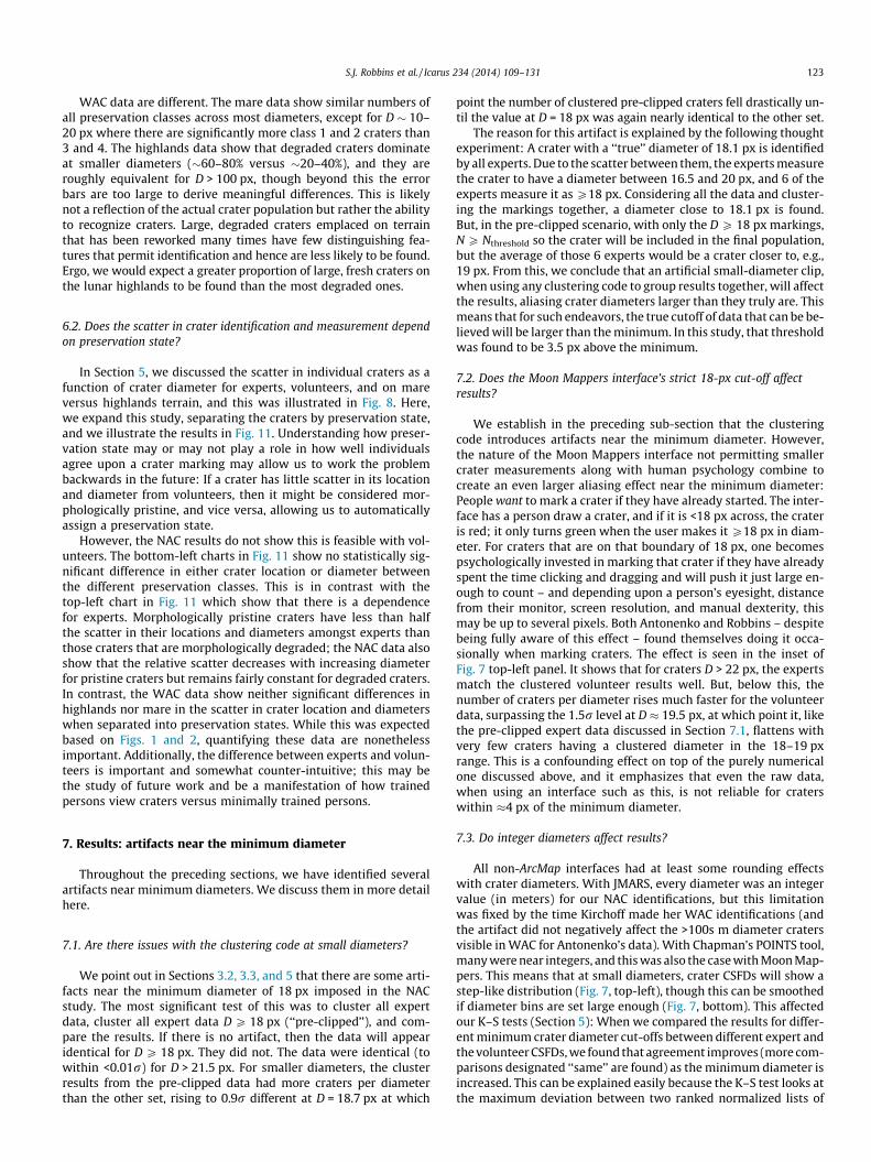
S.J. Robbins et al. / Icarus 234 (2014) 109–131 123

WAC data are different. The mare data show similar numbers ofall preservation classes across most diameters, except for D � 10–20 px where there are significantly more class 1 and 2 craters than3 and 4. The highlands data show that degraded craters dominateat smaller diameters (�60–80% versus �20–40%), and they areroughly equivalent for D > 100 px, though beyond this the errorbars are too large to derive meaningful differences. This is likelynot a reflection of the actual crater population but rather the abilityto recognize craters. Large, degraded craters emplaced on terrainthat has been reworked many times have few distinguishing fea-tures that permit identification and hence are less likely to be found.Ergo, we would expect a greater proportion of large, fresh craters onthe lunar highlands to be found than the most degraded ones.

6.2. Does the scatter in crater identification and measurement dependon preservation state?

In Section 5, we discussed the scatter in individual craters as afunction of crater diameter for experts, volunteers, and on mareversus highlands terrain, and this was illustrated in Fig. 8. Here,we expand this study, separating the craters by preservation state,and we illustrate the results in Fig. 11. Understanding how preser-vation state may or may not play a role in how well individualsagree upon a crater marking may allow us to work the problembackwards in the future: If a crater has little scatter in its locationand diameter from volunteers, then it might be considered mor-phologically pristine, and vice versa, allowing us to automaticallyassign a preservation state.

However, the NAC results do not show this is feasible with vol-unteers. The bottom-left charts in Fig. 11 show no statistically sig-nificant difference in either crater location or diameter betweenthe different preservation classes. This is in contrast with thetop-left chart in Fig. 11 which show that there is a dependencefor experts. Morphologically pristine craters have less than halfthe scatter in their locations and diameters amongst experts thanthose craters that are morphologically degraded; the NAC data alsoshow that the relative scatter decreases with increasing diameterfor pristine craters but remains fairly constant for degraded craters.In contrast, the WAC data show neither significant differences inhighlands nor mare in the scatter in crater location and diameterswhen separated into preservation states. While this was expectedbased on Figs. 1 and 2, quantifying these data are nonethelessimportant. Additionally, the difference between experts and volun-teers is important and somewhat counter-intuitive; this may bethe study of future work and be a manifestation of how trainedpersons view craters versus minimally trained persons.

7. Results: artifacts near the minimum diameter

Throughout the preceding sections, we have identified severalartifacts near minimum diameters. We discuss them in more detailhere.

7.1. Are there issues with the clustering code at small diameters?

We point out in Sections 3.2, 3.3, and 5 that there are some arti-facts near the minimum diameter of 18 px imposed in the NACstudy. The most significant test of this was to cluster all expertdata, cluster all expert data D P 18 px (‘‘pre-clipped’’), and com-pare the results. If there is no artifact, then the data will appearidentical for D P 18 px. They did not. The data were identical (towithin <0.01r) for D > 21.5 px. For smaller diameters, the clusterresults from the pre-clipped data had more craters per diameterthan the other set, rising to 0.9r different at D = 18.7 px at which

point the number of clustered pre-clipped craters fell drastically un-til the value at D = 18 px was again nearly identical to the other set.

The reason for this artifact is explained by the following thoughtexperiment: A crater with a ‘‘true’’ diameter of 18.1 px is identifiedby all experts. Due to the scatter between them, the experts measurethe crater to have a diameter between 16.5 and 20 px, and 6 of theexperts measure it as P18 px. Considering all the data and cluster-ing the markings together, a diameter close to 18.1 px is found.But, in the pre-clipped scenario, with only the D P 18 px markings,N P Nthreshold so the crater will be included in the final population,but the average of those 6 experts would be a crater closer to, e.g.,19 px. From this, we conclude that an artificial small-diameter clip,when using any clustering code to group results together, will affectthe results, aliasing crater diameters larger than they truly are. Thismeans that for such endeavors, the true cutoff of data that can be be-lieved will be larger than the minimum. In this study, that thresholdwas found to be 3.5 px above the minimum.

7.2. Does the Moon Mappers interface’s strict 18-px cut-off affectresults?

We establish in the preceding sub-section that the clusteringcode introduces artifacts near the minimum diameter. However,the nature of the Moon Mappers interface not permitting smallercrater measurements along with human psychology combine tocreate an even larger aliasing effect near the minimum diameter:People want to mark a crater if they have already started. The inter-face has a person draw a crater, and if it is <18 px across, the crateris red; it only turns green when the user makes it P18 px in diam-eter. For craters that are on that boundary of 18 px, one becomespsychologically invested in marking that crater if they have alreadyspent the time clicking and dragging and will push it just large en-ough to count – and depending upon a person’s eyesight, distancefrom their monitor, screen resolution, and manual dexterity, thismay be up to several pixels. Both Antonenko and Robbins – despitebeing fully aware of this effect – found themselves doing it occa-sionally when marking craters. The effect is seen in the inset ofFig. 7 top-left panel. It shows that for craters D > 22 px, the expertsmatch the clustered volunteer results well. But, below this, thenumber of craters per diameter rises much faster for the volunteerdata, surpassing the 1.5r level at D � 19.5 px, at which point it, likethe pre-clipped expert data discussed in Section 7.1, flattens withvery few craters having a clustered diameter in the 18–19 pxrange. This is a confounding effect on top of the purely numericalone discussed above, and it emphasizes that even the raw data,when using an interface such as this, is not reliable for craterswithin �4 px of the minimum diameter.

7.3. Do integer diameters affect results?

All non-ArcMap interfaces had at least some rounding effectswith crater diameters. With JMARS, every diameter was an integervalue (in meters) for our NAC identifications, but this limitationwas fixed by the time Kirchoff made her WAC identifications (andthe artifact did not negatively affect the >100s m diameter cratersvisible in WAC for Antonenko’s data). With Chapman’s POINTS tool,many were near integers, and this was also the case with Moon Map-pers. This means that at small diameters, crater CSFDs will show astep-like distribution (Fig. 7, top-left), though this can be smoothedif diameter bins are set large enough (Fig. 7, bottom). This affectedour K–S tests (Section 5): When we compared the results for differ-ent minimum crater diameter cut-offs between different expert andthe volunteer CSFDs, we found that agreement improves (more com-parisons designated ‘‘same’’ are found) as the minimum diameter isincreased. This can be explained easily because the K–S test looks atthe maximum deviation between two ranked normalized lists of

Fig. 11. Similar to Fig. 8, but this Figure expands those data by preservation class. The left column are NAC data, right column are WAC data. Each set of four are the samecategory of data (persons, area/data) but the top group are locations and bottom group are diameters. In each set of four, the top-left are experts and bottom-left arevolunteers. WAC data have been divided by mare (top right) and highlands (bottom right); the diameter range has been limited for the WAC data because all larger bins havefewer than 5 craters in them. Note that the horizontal axes are different between the two columns because of different completeness limits.

124 S.J. Robbins et al. / Icarus 234 (2014) 109–131

data, and since the most craters are at small diameters, the largestdifferences will be found between the smallest craters from JMARSversus other interfaces.

7.4. How did each expert measure and ensure completeness?

Each expert was asked to provide NAC image crater counts forall craters D P 18 px and WAC counts to diameters ‘‘you are com-

fortable identifying.’’ In every case for the former, each person saidthey identified craters several pixels smaller than the 18-px cut-offto assure completeness (the diameter to which we estimate that allcraters were identified), and other than clustering and roundingartifacts, this was found to be an accurate method. We concludefrom this that, if one is trying to ensure completeness to a certainminimum diameter Dmin (i.e., they have included all cratersPDmin), an individual should actually attempt to be complete to

S.J. Robbins et al. / Icarus 234 (2014) 109–131 125

diameters a �few px smaller than Dmin. Conversely, if they thinkthey are complete to a certain diameter, it is likely they havemissed some craters, and Dmin is a few pixels larger.

The WAC experiment represented a very different case, andeach person had a slightly different technique to estimate thesmallest diameter to which they thought all craters were included(completeness):

� Antonenko: Estimated based on the maximum value in a �100-m size bin on an incremental SFD. For her ArcGIS data, this is400 m ( J 7 px), and for her JMARS data, this is 300 m ( J 6 px)� Chapman: A priori estimate of �12 px could be achieved, so

measured down to 9–10 px (�600 m) to ensure this.� Fassett: General ‘‘comfort’’ through experience, estimated at

700 m ( J 11 px).� Herrick: 8–10 px, visually estimated a priori, and so craters were

measured to �8 px. He then looked at where the CSFD divergedfrom a straight line (on log–log axes) which was estimated as600 m ( J 9–10 px) after counts were completed.� Kirchoff: Measured craters down to 5 pixels across and then

examined a CSFD of her data and looked for where the CSFDdiverged from a straight line (on log–log axes). Estimated tobe 350 m ( J 5.5 px) though cautioned this may be misleading.� Robbins: Created an incremental SFD in 21/8D multiplicative

intervals, looked for the diameter bin with the largest numberof craters, and estimated completeness to be the diameter binone larger than that. Also did this for individual 1000 �1000 px latitude � longitude bins. Most of the image was ‘‘com-plete’’ to 6–7 px, but the maximum was 9 px.� Singer: Normally would map no smaller than �5 px, but felt fea-

tures as small as �4 px could be identified in the mare region.Thus, she counted craters this small in the initial mapping andchecked the small-diameter roll off in the SFDs later to estimatea completeness of �5–6 px.� Zanetti: Estimated completeness to be �500 m ( J 8–9 px) in

the mare area but due to the significant jumbled terrain, placeda very conservative completeness estimate of �1 km ( J 15–16 px) in the highlands. These were estimated by comfort level.

These estimates are illustrated in Fig. 7 as small arrows on theCSFDs in the WAC panels. With the reduced dataset, we can com-pare these estimates and determine their accuracy relative to theensemble. Chapman’s, Fassett’s, and Robbins’ data overall and Kirc-hoff’s mare counts show they under-estimated completeness (theywere complete to smaller diameters than predicted) by a few pix-els. Kirchoff’s highlands, both Antonenko’s ArcGIS and JMARS mareand JMARS highlands, Herrick’s mare, and Singer’s mare countsshow they had a good estimate of their completeness. Singer’s few-er craters by a factor of 2� in the highlands relative to the ensem-ble show that she consistently under-counted craters relative tothe ensemble, though the relative population was complete tothe diameters she estimated (K–S test showed they are the samepopulation). Herrick’s estimate of complete counts for D P 9 pxis also an over-estimate, for his counts have a shallower slope thatdeviates from the rest for D < 15 px which is the start of his lack ofcomplete data. The CSFD slope of Antonenko’s ArcGIS highlandscounts begins to shallow relative to the other data for D < 10 px in-stead of her estimated �7 px completeness.

In the above bulleted list, it is clear that there are several differ-ent qualitative and quantitative methods employed by differentindividuals. With the criterion that the most conservative is thebest estimate, Fassett’s qualitative ‘‘gut feeling’’ was about as goodas Robbins’ complicated quantitative method. More concerning isthe change in slopes near each person’s minimum diameter, whereHerrick’s counts fall well below others’ for �6 px larger than hisestimated completeness. Unfortunately, this is not the only kind

of artifact observed: Both Kirchoff’s and Robbins’ highlands datainstead show a steeper slope for D < 10 px and D < 9 px, respec-tively, relative to the ensemble results, indicating a possible alias-ing effect to larger diameters. These effects were not dependent onthe interface used to identify and measure craters.

Unfortunately, without counts in the region to even smallerdiameters or a comparable dataset, it is not possible to state withabsolute certainty the completeness of any one person’s cratercounts, and limitations in funding and time and the tediousnessof identifying craters is a barrier to multiple experts wanting toduplicate another’s counts. It is also probable that in any singleperson’s crater counts anywhere near their estimated minimumdiameter, any deviation from an expected crater population caneasily be an artifact of being near that minimum, especially if itis fewer than 10 px in the image data that is being used. Extremecaution and a conservative approach are recommended near anyminimum diameter estimate.

8. Results: biases causing the primary differences amongexperts and between experts and volunteers

All tools except for the Moon Mappers interface are designed byprofessionals for professionals. Therefore, the largest a priori biasesare likely to result from the MM interface versus the other inter-faces. And, barring bugs (i.e., JMARS rounding issue), this was thecase based on previous sections.

In the quest for a simple interface that provides the minimumlearning curve, the MM marking tool lacks many of the imagemanipulation methods available to professionals. For example,the ability to zoom in and out – i.e. over- or under-samplingthe image on-screen – is not available unless computer operatingsystem- or internet browser-specific manipulations are enabled topermit one to zoom in. This could potentially result in less exactmarkings than desired, or more time might be needed to achievethe same desired precision. The interface also does not allow oneto move a fraction of an image to the side, forcing one to some-times identify only partial craters (however, the interface onlyallows one to identify craters where >50% is visible). While theimage location is one type of limitation, a second is the way inwhich the image is displayed. As shown in Table A2, all expertsin this project made use of image display modifications – be itindividually or a combination of contrast, curves, gamma, greyscaleinversion, brightness changes, or rotation – in order to enhance lo-cal topography differences to assist in crater identification. Thesetools are lacking in MM and so it is very much a ‘‘what you seeis what you get’’ interface. Despite the inability to perform any im-age manipulation, the above analyses show that volunteers per-formed remarkably well as an ensemble in comparison with theexperts as an ensemble. The interface was found to speed upcounts by Antonenko while slow down counts by Robbins, buttheir results were comparable to their other techniques.

9. Discussion and conclusions

This represents the first extensive study focused on understand-ing the difference in crater identification and measurement be-tween numerous, independent crater experts using a variety ofmethods, and between those experts and lay volunteers. Through-out this work, we quantified several different comparisons andreached several conclusions:

1. We found anywhere from a ±10% to ±35% dispersion amongexperts in the number of craters found in different size bins,even when the numbers were many 10s or 100s of craters,and the crater diameters were well above the minimum

126 S.J. Robbins et al. / Icarus 234 (2014) 109–131

diameter studied. This dispersion is dependent on the simplic-ity of the terrain with �km-scale mare craters being the mostconsistent and the heavily modified lunar highlands the mostvaried.

2. The Moon Mappers online interface, despite its simplicity,yields results that are statistically as good as professionallydeveloped interfaces for identifying craters, though artifactsare present within a few pixels of the minimum diameter(which could be eliminated by removing the minimum diame-ter or limiting studies to a few pixels larger than the minimum).

3. Except near the minimum diameter, volunteers are able toidentify craters just as well as the experts (on average) whenusing the same interface (the Moon Mappers interface), result-ing in not only a similar number of craters, but also a similarsize distribution. This analysis was for the Nthreshold = 4 and 5for experts (depending on number of datasets per image) andmay vary if Nthreshold were different.

4. An a priori assumption that was nonetheless verified is that thelunar highlands crater counts are most prone to uncertainty –especially at660� solar incidence – of the three types and scalesof terrains studied, but the experts were conscious of this andplaced caution on their exact crater counts. However, whilefuture work may show this to be valid across a large numberof sample terrains, it is technically valid only for this particularimage set.

5. Experts and the individual volunteers differ significantly in thatmost experts found every crater that made it into the final cat-alog, but exponentially fewer volunteers found more cratersthat were in their final catalog.

6. Experts are more consistent among each other in crater mea-surement and identification and are better at identifyingdegraded craters than volunteers: The scatter in location anddiameter is around 5–10% and decreased with better preservedcraters, but for volunteers, the scatter between individuals isapproximately ±10% for location and ±20% for diameter andwas mostly independent of crater preservation. There was nosignificant dependence on diameter. Ensemble crater diametersfound by volunteers and experts matched 1:1 within theiruncertainties.

7. Many artifacts occur near a minimum crater diameter, andexperts are mixed in their ability to accurately assess their min-imum completeness diameter. When the minimum diameter iswell over 10 px, experts are able to consistently return com-plete counts by attempting to be complete to smaller diameters,but completeness at smaller than 10 px diameters returns arti-facts that depend upon the person – i.e., we found that somepeople identify more craters near that minimum, while othersidentify less. It is possible that different instructions (i.e., ‘‘Dataas accurate as possible for all D P 4 px craters are required forthis work’’) may have resulted in more consistent small-diame-ter results, but the phenomenon of different artifacts found indifferent researchers’ counts is still troublesome.

From these findings, we conclude that volunteers are approxi-mately as good as experts in identifying craters, at least on terrainof ‘‘mixed’’ difficulty, so long as enough volunteers examine theimage to derive a robust result (e.g., at least 15 persons view theimage; where this value may reach a point of diminishing returnswill be the subject of future work). This finding is also with thecaveats that (a) one should be interested in using the craters asan overall population as opposed to needing highly accurate resultson just an individual or a few individual craters, and (b) they arewilling to use craters a few pixels larger than the minimum iden-tified by volunteers. From this work, we can also strongly recom-mend that researchers be cautious when using craters <10 px indiameter, especially in using small deviations from an expected

function to conclude secondary crater contamination or cratererasure.

The variation in the number of craters identified by the expertson the same terrain has implications for interpretations that makeassumptions about crater detectability. For example, Richardson(2009) modeled crater saturation, but inherent in that model is adetectability threshold to decide when a crater is sufficiently de-graded or overprinted to be uncountable. Our data show that thisthreshold varies among experts. This factor is relevant to the long-standing debate about whether the heavily cratered terrains on theMoon and other planetary bodies are in saturation (Gault, 1970;Woronow, 1977, 1985; Hartmann, 1984; Squyres et al., 1997;Richardson, 2009). While this is one example, the broader implica-tion is that this variability would affect chronological informationderived from complex surfaces, especially on more degradedterrain (e.g., the lunar highlands).

With the caveat that secondary craters were not excluded, theextreme spread among experts in our example WAC highlandsregion at the 1-km-diameter point (where the lunar chronologyis defined) is a factor of 4.5. Note, however, that all Poisson errorbars in the counts overlap with at least one other expert’s dataexcept for Chapman’s and Singer’s (D = 1 km = 15.5 px, where therelative standard deviation is ±38% (Fig. 4)). While this work wasnot meant to derive model ages, we can look at the implicationsof it as applied to that process. The crater densities equate to acrater retention age of between 3.4 ± 0.1 and 3.8 ± 0.0 Gyr,while the ensemble is 3.7 ± 0.0 Gyr (under the Hartmann (1999)system using the Ivanov (2001) chronology). The mare terrain,despite the overall agreement being better among experts, atD = 1 km has a density variation of 2.6. Due to the youth of thisterrain, the resulting variation in ages is wider, from 1.3 ± 0.4 to2.2 ± 0.5 Gyr, while the ensemble is 1.7 ± 0.4 Gyr (the relativestandard deviation is ±16% at this diameter, and all experts’error bars overlap each other (Fig. 4)). To add to the list ofconclusions:

8. Age uncertainties based on counting statistics almost alwaysare artificially small because they neglect natural variations ina single analyst’s threshold of detection and the even largervariations expected for other expert analysts. Small differencesin crater density between units measured by the same analystmay be real, but absolute ages based on an analyst’s measuredcrater densities must be regarded as being subject to uncertain-ties at least as large as a factor of ±20% and even larger (>±35%)for difficult terrains such as lunar highlands.

The difference in the NAC data at 150 m (the smallest diameterthat is not saturated, �220 px) is a factor of 2.3 between the min-imum and maximum expert data. These correspond to ages of1.5 ± 0.7 to 3.2 ± 0.8 Gyr. However, the variation between volun-teers’ and experts’ ensemble results at this diameter is only a factorof 1.01 relative to each other, corresponding to an age estimate of2:71þ0:89

�0:91 to 2:72þ0:89�0:91 Gyr (three significant figures only used to

illustrate the degree of similarity). While the error bars are quitelarge (few craters were D P 150 m, P220 px in the NAC studyarea), this still shows significant variation on the order of at leastseveral hundred million years is possible between mappers; wealso found density variation to be generally greater than the factorof 2 which is inherent in the chronology function itself. Two addi-tional conclusions can be drawn from this exercise.

9. It is not appropriate to quote model crater ages to three ormore significant figures (though several of the authors of thispaper are guilty of doing so, and we do so in the one compar-ison case above to show the excellent agreement). We recom-mend only using two significant figures.

S.J. Robbins et al. / Icarus 234 (2014) 109–131 127

10. Volunteers appear to be able to provide an ensemble result forage modeling as good as experts – despite the inherent uncer-tainties discussed throughout Sections 3–8 – in light of the lar-ger uncertainties inherent to most applications of craterpopulations (such as age modeling).

The analysis presented in this work relied on a clustering algo-rithm and setting an Nthreshold of the number of persons who musthave identified a crater for it to be included in the ‘‘ensemble’’ cat-alog. For the experts, we set this at approximately half the num-ber of datasets we had assembled. However, one could plausiblyargue that Nthreshold should be set to a smaller number, such as2, or a larger number. Changing the value will alter the numberof craters in the final catalog, and raising or lowering it wouldrepresent two different philosophies: If one requires feweranalysts to have found the crater, then this could be interpretedas it being unlikely that two people would independently findthe same ‘‘non-crater’’ and it is more likely that others simplymissed it. At the other extreme, requiring more people to havefound the feature for it to count takes a more conservativeapproach where one would want to be much more certain the fea-ture is truly a crater before adding it to a final catalog. Each hastheir own separate uses, and one should select an Nthreshold thatis most appropriate for their application. In this work, we usedNthreshold � 0.5Nexperts so as to not weight any one analyst morethan others and produce a catalog of craters that the ‘‘average’’analyst should find. The number of craters we identified with thisNthreshold value is almost certainly less than the objective reality inthat there will be craters that are physically present that mostpersons will not find, and perhaps no analyst could find. But, wethink this represents a reasonable consensus of the crater popula-tion for these surfaces.

This study presents the most vetted catalog of craters on twotargeted regions of the lunar surface with a range of morphol-ogy. This kind of data product is useful as a training set for indi-viduals learning how to identify craters, calibrating themselves,and for training automated crater detection codes. As a resourcefor those communities, we have made these data and imagesavailable as a Supplemental material with this paper, andwe encourage the reader to contact the first author for moredetails.

While this work has focused on the Moon, we expect that its re-sults are applicable to at least other airless bodies and likely to allplanetary surfaces in general because crater identification andmeasurement requires similar skills from one surface to another.The main consideration for applying these results to other worldswould be to account for the role of active geological processes thataffect craters in various ways and whether there are other endo-genic processes (e.g., collapse pits) that mimic the appearance ofimpact craters. Additionally, different gravity fields and extremelocal slopes can alter crater morphology. For example, Mars hasfluvial and aeolian processes to consider when determiningwhether a feature is a degraded crater, and Asteroid (4) Vestahas numerous craters emplaced on steep slopes that result inhighly asymmetric features that an untrained person may not rec-ognize as an impact crater. Two Venusian crater catalogs con-structed in the 1990s (Schaber et al., 1992; Herrick and Phillips,1994) had differences based on what each group considered an im-pact crater versus a volcanic structure, a difficulty enhanced byatmospheric fragmentation clustered smaller impact craters to-gether, forming irregular features that were easily mistaken forirregular volcanic calderas. Overall, however, the lessons learnedfrom this work on lunar craters should be applicable to most plan-etary bodies, and the same cautions and considerations should beapplied.

Acknowledgments

The authors thank two anonymous reviewers for their helpfulfeedback. Support for Robbins was through the Maryland SpaceGrant Consortium and the NASA Lunar Science Institute Central of-fice. Support for Kirchoff and Chapman was through the Center forLunar Origin and Evolution node of the NASA Lunar Science Insti-tute. Support for Zanetti was through the McDonnell Center forSpace Science, Lawrence Haskin Memorial Fellowship. Supportfor Lehan, Huang, and Gay was through support for CosmoQuestby National Aeronautics and Space Administration GrantsNNX09AD34G and NNX12AB92G, STScI under National Aeronau-tics and Space Administration Contract NAS 5-26555, and fundingthrough the Lunar Reconnaissance Orbiter education and public out-reach office.

Appendix A. Details of crater identification and measurementmethods

Most of the researchers in this study used different interfacesand measurement techniques. They are described briefly in Sec-tion 2.2 and in depth in this Appendix.

A.1. ArcGIS

ArcGIS software, produced by ESRI, is a popular suite in thegeology field and contains numerous tools and add-on softwarethat are useful in analyzing geographic datasets and annotatingthem. The majority of experts in this study used ArcGIS software,though four distinct methods were employed within the ArcMapsoftware application.

A.1.1. Rim-TracingRobbins was one of two researchers to use the native tools

within ArcMap. His technique is more thoroughly described in Rob-bins and Hynek (2012), but briefly, each image was imported intoan empty ArcMap file without any ancillary projection files (i.e., thePGW file – PNG World file – was removed). This forced ArcMap totreat the image as being in pixel space. He used ArcMap’s Editingtools in ‘‘streaming’’ mode to lay down a vertex every 2.5 pixels– this was chosen because it would be about 20 points along therim of the smallest crater (on NAC), and it allowed him to not bepixel-perfect in vertex deposition. The vertex spacing was de-creased to permit smaller crater identification on the WAC image.He then traced every crater rim using a Wacom tablet and pen asan input device. These were saved to a GIS shapefile and, when fin-ished, exported as a text file in units of pixels. He then used customsoftware to fit both circles and ellipses to each crater rim.

Robbins was the fastest crater identifier in this study, probablyfor two reasons. First, he uses a pen/tablet input device, allowing amore natural drawing capability; he was one of only two research-ers in this study to use a pen (Singer was the other, and her iden-tifications were second-fastest). Second, he traces crater rimswhich is simply an act of drawing a circle with the pen and press-ing the ‘‘F2’’ or a software-assigned button on the tablet to closethe circle. He can then immediately move onto the next crater withless than one second pause between. In this way, he does not haveto worry about how a three-point fit looks nor manually click threeor more points along the rim, it’s simply draw-and-click, draw-and-click, etc.

A.1.2. CraterToolsThe CraterTools extension to ArcMap was released by Kneissl

et al. (2011). It includes a three-point tool that fits circles similar

128 S.J. Robbins et al. / Icarus 234 (2014) 109–131

to other interfaces discussed in this Appendix: The researchermanually identifies three points along the rim and then Crater-Tools fits a circle and records that in a GIS shapefile.

Fassett’s modification to this was to overlay a grid on top of theimage at �70% the minimum diameter desired. Any crater that issmaller than a single grid cell is ignored.

A.1.3. Crater Helper ToolsThis USGS extension to ArcMap was used by Antonenko and

Herrick to manually identify craters (Herrick used this for theNAC exercise and CraterTools for WAC). Craters are identified byclicking three points on the rim, which uniquely identifies a circle.In all cases, craters were fit with a circle, and the center point anddiameter of the circle are then provided by the software.

A.1.4. Chord-DrawingSinger also used the native tools in ArcMap to map craters with

an additional extension to calculate spherical lengths (Tools forGraphics and Shapes (Jenness, 2011)). Crater diameters were mea-sured by drawing a straight line from one rim to another (one pointon each side), going through the center of the crater, with an at-tempt at consistency about orientation of the line with respect tothe lighting geometry (bisecting the shadow in most cases). Thiswill likely give the most accurate estimate of the diameter. Theremay be some advantages and disadvantages of this technique ascompared to those that fit circles to a number of points on therim – it might seem that precision could be sacrificed for speed.From a visual assessment of Figs. 1 and 2, however, there is noobvious trend for craters mapped this way to be consistently offfrom the overall average. Large discrepancies between mappeddiameters may be due to individual discretion about the locationof the rim, especially for degraded craters. One advantage may bethat measurements were made relatively consistently with respectto lighting geometry which may or may not be the case whenmarking three points on a rim via other techniques. Singer alsomade use of a tablet and pen input device.

A.2. JMARS

JMARS is a tool produced and maintained by Arizona State Uni-versity that many use as a free alternative to ArcGIS software fordisplaying planetary datasets. It has a built-in crater-measuringtool. Craters are identified visually and the ‘‘Three Point Mode’’ ofthe tool was used by Kirchoff. Three points along the identifiedrim are manually selected and then the circle-fit calculation is per-formed by JMARS. Antonenko used the circle-drawing tool con-tained within JMARS which is a similar method to the MoonMappers interface. Craters are digitally recorded by JMARS with acenter latitude and longitude in degrees and diameter in meters.A minimum size can be set through the use of a smaller-than-min-imum template (the ‘‘Add Mode’’ in the JMARS crater countingtool) to determine which craters are equal to or larger than thisdiameter.

A limit of the version of JMARS prior to early April 2013 wasthat crater diameters were rounded to the nearest integer mea-surement (meter) when using the 3-point and circle-drawing tools(sub-meter measurements can be made with the ‘‘add’’ tool),although locations are not rounded. This caused aliasing in thesmall-diameter range in later analysis. The maintainers of JMARSwere aware of this issue and fixed it in early April 2013 – too latefor the NAC data, but in time for Kirchoff’s WAC data.

A.3. SAOImage DS9

The DS9 interface was used by Chapman in conjunction withPeter Tamblyn’s crater measurement program (written in Perl

and running on Windows XP, with subroutines from the POINTSsoftware developed at Cornell by J. Joseph and P. Thomas in the late1990s). The crater measurement loop works as follows: The mea-surer positions the tip of the cursor arrow at a point on the rimof a crater and clicks it, producing an X-shaped mark; this is done2, 4, 6, or more times (3 and 5 times do not work). After markingthe rim, the measurer moves the cursor to a small window, clickswithin it to make it active, types ‘‘f’’ and a number from 1 to 4 (rep-resenting the morphology classification estimated by the mea-surer), hits carriage return, then ‘‘l’’. At this time, the X’s in themain image are replaced with the fitted ellipse. The {x, y} positionand semi-major and –minor axes are written to a data file. If an er-ror is perceived, there are buttons in the ‘‘craters’’ window that canchange the shape, size, and position of the fitted ellipse (very rarelyused); alternatively, the crater can be deleted and a new set of rimmeasurements made from scratch (such deletions cause gaps inthe crater numbering). With the cursor positioned on the rim ofthe next crater, a click begins the process for the next crater.

There is a coding issue when a crater is being measured thatoverlaps, or lies within, a previously measured crater. There is an‘‘overlay on/off’’ button that changes the measurement mode sothat it works; the cursor has a different appearance, but otherwiseis the same from the measurer’s perspective. The DS9 viewer win-dow can be zoomed in or out by a factor of two in scale, althoughmeasurements can be made only in zoom = 1, 2, 4, etc. (not ½, 1=4,etc.). At larger zoom values, the position of the measurement win-dow can be adjusted to the correct part of the whole image using asmall window that shows the viewed portion in a blue rectangle.With the right button pressed, dragging the cursor around the im-age can change the brightness and contrast of the image, whichespecially affects the visibility of shallow craters.

A.4. Moon Mappers interface

The Moon Mappers interface was used exclusively by volun-teers. For comparison purposes, both Antonenko and Robbins (sci-ence co-leads on Moon Mappers) also used this interface todetermine if there were significant differences between it and theirpreferred method.

This is an internet-based interface. After logging in at cosmo-quest.org, volunteers select the ‘‘Moon Mappers’’ application andcan choose a ‘‘Simply Craters’’ or ‘‘Man versus Machine’’ interface.In the latter, images have pre-marked craters overlaid from anautomated crater detection code; craters identified within thatinterface were excluded from this analysis because this approachdid not match the process used by experts and would have addedcomplexity to the comparison. For both interfaces, images are pre-pared by a sub-dividing code. First, the NAC image is scaled to100%, 33%, and 11% size (1 � 1, 3 � 3, and 9 � 9 pixel binning).Each scaled NAC is then divided into 450 � 450-pixel sub-imageswith a minimum of 30 pixels overlap on the edges. This is meantto ensure that no portion of an image is missed and that they areviewed at multiple scales. For the portion of the M146959973L im-age used in this study, only 1 � 1 and 3 � 3 binning was appliedbecause of the small width of the study region.

Within the MM online interface, each sub-image is displayed tothe volunteer one at a time in quasi-random order. The interfacehas a basic crater-marking tool that allows the user to draw a circleby clicking at the crater center and dragging outwards. The circle isred until it reaches the minimum diameter of 18 pixels, and then itturns green. If the mouse button is released while the circle is red,it does not save; green, it does. The volunteer can use another toolto reposition the final circle and resize it. Users can mark craters assmall as 18 pixels across or as large as 450 pixels across. Whenthey are satisfied they have annotated all D P 18 px craters on

S.J. Robbins et al. / Icarus 234 (2014) 109–131 129

an image, a ‘‘Done Working’’ button is pressed and the craters aresaved to an online database.

Appendix B. Details of researcher experience

One of the primary purposes of this study is to identify variationin crater identification among experts. This Appendix providesbrief biographical notes about each researcher that focuses on theircrater identification experience. Researchers are listed alphabeti-cally by surname, not in author order.

Antonenko has over 20 years experience in identifying andmeasuring craters on the Moon, using a variety of data sets, reso-lutions, and lightning conditions to determine the sub-surface stra-tigraphy revealed by impact craters. Other work by Antonenko hasalso involved studying craters on Venus, Ganymede, and the Earth.Antonenko, along with Robbins, is Science co-Lead for MoonMappers.

Chapman began measuring craters within weeks of graduatinghigh school in 1962, and he has had experience measuring craterson ten bodies (Moon, Mars, Gaspra, Ida, Europa, Ganymede, Cal-listo, Mathilde, Eros, Mercury), in recent decades as a member ofnumerous spacecraft science teams. With a career in this workspanning over five decades, he is the most senior researcher in-volved in this work and has used the broadest range of datasets(quality, surface, medium) and techniques.

Fassett has eight years (since 2006) experience measuring cra-ters. Along with Seth Kadish, he constructed a catalog of �15,000craters with D P 20 km on Mercury and the Moon. A counter-pointto this experience is that he almost never works with craters smal-ler than 100 m, as emphasized in Table A1 where he considers theNAC image both difficult and of little chronologic utility because ofits saturated state.

Herrick has been involved in impact cratering studies for�20 years. He participated in creating the first global catalog ofVenusian craters using radar images from the Magellan mission,and he has catalogued craters on other planetary bodies for variousresearch tasks.

Kirchoff has seven years (since 2007) experience identifyingcraters on various surfaces including the Moon, Mars, and icy sat-ellites of Jupiter and Saturn. This work has helped determine thegeologic and bombardment histories of these bodies while alsogenerating global crater databases for several icy satellites ofSaturn.

Robbins has seven years (since 2007) experience identifyingcraters on inner Solar System bodies with most work focusing onMars. He manually constructed a �640,000 martian crater data-base, published in 2012 (Robbins and Hynek, 2012) and has

Table A1Key data on crater identification for each expert for both the NAC and WAC images.

Researcher Time to analyze NAC (h) Time to analyze WAC (h) N P 18 px N

Antonenko 5.5a, 7b, 4c 5a, 5.5b 636a, 996b, 6Chapman 12e 4.55 1197Fassett 5.7 3 814Herrick 8 3 808Kirchoff 6 7 1027Robbins 2.4d, 4.5c 1.4 1060d, 991c

Singer 3 2 652Zanetti 7 2.5 930

a Data analysis conducted in/with: Crater Helper Tools.b Data analysis conducted in/with: JMARS.c Data analysis conducted in/with: Moon Mappers.d Data analysis conducted in/with: Rim-Tracing in ArcMap.e Chapman also measured degradation state so this increased the time spent.f Except for numerous heavily degraded craters.

worked on similar analyses on lunar craters. Along with Anton-enko, Robbins is Science co-Lead for Moon Mappers.

Singer has seven years (since 2007) experience mapping andmeasuring various geologic features (circular or otherwise) onthe icy satellites in the outer Solar System. This includes craterson various bodies (Europa, Ganymede, Enceladus, and Triton) aswell as other geologic features on Europa (sub-circular chaos, pits,uplifts) and Iapetus (lineaments and long-runout landslides).

Zanetti has six years (since 2008) experience studying the for-mation and degradation of impact craters on the Moon, Mars, andEarth and has counted craters on volcanic structures and craterejecta blankets using high resolution LROC NAC images of theMoon (Zanetti et al., 2013) and HiRISE images of young surfaceson Mars.

Appendix C. Details of crater clustering code

In this Appendix, we detail how our clustering code works toautomatically group features into single craters. We started fromthe basic two-dimensional DBSCAN algorithm of Ester et al.(1996). The original DBSCAN code was developed to (a) require aminimum amount of a priori knowledge (represented by a mini-mum number of input parameters), (b) identify clusters of arbi-trary shape, and (c) scale well with large datasets. This algorithmwas chosen over other potential codes (such as expectation–max-imization (EM) clustering) because of the nature of our data: Thedensity of crater markings varies as a function of feature size (withlarger features having more absolute spread) and sets of markingshave a small sample size (�15 volunteers view each image) thatare not necessarily normally distributed. The original DBSCANalgorithm hinges on the idea of ‘‘reachability,’’ where one datumis considered ‘‘reachable’’ by another if its location is within a dis-tance e specified a priori by the user. If enough points are reachableby each other, they are considered to be members of a cluster. Theminimum number of points (Nthreshold) needed to be considered acluster is also pre-defined by the user.

The advantage of DBSCAN is that the algorithm is straightfor-ward, easy to implement, and it is accurate enough for the nextstep – the science analysis. However, a drawback is the time com-plexity (how long the code takes to run) which is OðN3Þ. First, iter-ating through each point in the dataset in order to find matchestakes OðNÞ. The search to find reachable points by the point inquestion is another OðNÞ. If a reachable point is found, since otherpoints not previously reachable may now be reachable by the lar-ger cluster, the code must again search through every point whichadds another OðNÞ that brings the total time complexity to OðN3Þ.Due to the large datasets that we currently have and which we

AC craters Nall WAC craters NAC image difficult? WAC image difficult?

53c 949a, 1308b No Yes644 No Highlands1245 Yes No336 Yes Yes1633 No No1114 Yes No1036 Nof No1204 Yes No

Table A2Additional image manipulation performed by the different researchers using their preferred interface of choice.

Researcher Technique Changed pixel scale (zoom in/out) Contrast/brightness adjustment Rotation

Antonenkoa Crater Helper Tools (ArcMap) and JMARS X X (WAC only) [No]Chapman DS9 X X (WAC only) X (NAC)Fassett CraterTools (ArcMap) X X [No]Herrick Crater Helper Tools (ArcMap, NAC) and CraterTools (ArcMap, WAC) X X [No]Kirchoff JMARS X X [No]Robbinsa Rim-Tracing (ArcMap) X X [No]Singer Chord-Drawing (ArcMap) X X [No]Zanetti CraterTools (ArcMap) X X [No]

a Also performed NAC counts with the Moon Mappers interface which did not allow these different manipulations.

130 S.J. Robbins et al. / Icarus 234 (2014) 109–131

anticipate generating as an outcome of our volunteers’ efforts, wehave implemented an indexing structure that decreases the timecomplexity.

DBSCAN, as originally formulated, is a two-dimensional algo-rithm that works only with {x, y} location data and compares thisto the distance threshold e. In our work, the reality of planetarysurface features requires diameter to be considered, as well. Thisallows us to correctly address situations such as when a small cra-ter is superposed on a larger crater. A traditional DBSCAN codewould merge these two features together because they are withineach others’ e reachability, but their diameters clearly distinguishthem as separate features.

In 2D DBSCAN codes, two points pi and pj are considered part ofthe same cluster as follows

if(distance(pi, pj) < e1) then pi and pj are clustered

To take into consideration both distance and diameter, we mod-ified the if() statement such that two points pi and pj are consideredpart of the same cluster when the following is true:

if((distance(pi, pj) < e1(Di + Dj)/2) and (|Di � Dj| < e2 min(Di,Dj)))

As before, the first criterion compares the distance betweenpoints pi and pj, and the user-defined e1 parameter, but in ourimplementation, this parameter is scaled by the average diametersof the two features in question. This scaling accounts for scatter infeature location that varies with feature size rather than being anabsolute measured value (e.g., scatter can be ±5 pixels for a 50-pix-el-diameter feature and ±10 pixels of a 100-pixel-diameter featurerather than ±5 pixels for both). The second criterion compares thefeature diameters – our third dimension – where the difference ofthe two diameters is compared with the smaller feature’s diametermultiplied by a second reachability parameter, e2. This second cri-terion needs to be a relative, non-dimensional term. Otherwise, e2

would need to be different for any given size crater (e.g., a 3-pixeldiameter difference from a �5-pixel-diameter crater would not beconsidered a match, but a 3-pixel diameter difference between�200-pixel-diameter craters is negligible and should be consid-ered a match).

We determined the optimum reachability parameters by exam-ining a large dataset from an automated crater detection output fora related project. This set contained approx. 150,000 crater mark-ings that reduced to 10,104 clustered craters and the minimumnumber of features in each cluster was Nthreshold P 5. To determinethe optimum parameters, first, the physical distance, in pixel space,was determined between one crater and every other crater in thedataset. For each crater pair considered, the distance was normal-ized by the average diameter of the two craters being compared. Ahistogram of the normalized distances was then plotted. Thisshowed a peak at values very close to 0 that decreased to a

minimum at 0.35–0.5, and it then rose to encompass more craters.This minimum was robust across different datasets from our pro-jects – including both the expert and volunteer data in this work.We interpret this as the large number of craters that have distancesvery close together are actual matches for the same crater, and thatthe histogram’s minimum is the maximum distance craters can beseparated before they are no longer likely to be in the same cluster.Ergo, this minimum of 0.5 was chosen as our reachability for dis-tance, e1.

Of the pairs for which e1 < 0.5, the non-dimensionalized diame-ter reachability parameter e2 was calculated:

e2 > jDi � Djj=minðDi;DjÞ ð1Þ

After much testing of this and numerous other potential non-dimensionalizations, this parameter was found to robustly deter-mine whether two craters that were within the e1 threshold forlocation should be members of the cluster if, conveniently,e2 < 0.5, as well. Since division is often more time-consuming thanmultiplication, this leads to the second part of our earlier pseudo-code: (|Di � Dj| < e2 min(Di, Dj)). It should be noted that the valueof e2 can vary up to �1.0 without significantly affecting the resultsfrom our data.

The inputs to the clustering code are a tab-separated list of cra-ter location {x, y}, diameters D, and confidence c. Confidence is ascale of 0–1 and used for MM volunteers to score how well eachvolunteer performed relative to expert markings (Robbins’) on cal-ibration images. For experts, we set c = 1. After completion, thedata output for each cluster of markings are: (a) weighted mean�x with standard deviation, dx; (b) weighted mean �y with standarddeviation, dy; (c) weighted mean D with standard deviation, dD; (d)number of points N in that cluster; and (e) weighted mean of theconfidence for the craters that went into that cluster, �c. All weightsare based on the confidence c.

Appendix D. Supplementary material

Supplementary data associated with this article can be found, inthe online version, at http://dx.doi.org/10.1016/j.icarus.2014.02.022.

References

Arthur, D.W.G., Agnieray, A.P., Horvath, R.A., Wood, C.A., Chapman, C.R., 1963. Thesystem of lunar craters, quadrant I. Comm. Lunar Planet. Lab. 2, #30.

Crater Analysis Techniques Working Group, 1979. Standard techniques forpresentation and analysis of crater size–frequency data. Icarus 37, 467–474.http://dx.doi.org/10.1016/0019-1035(79)90009-5.

Ester, M., Kriegel, H.-P., Sander, J., Xu, X., 1996. A density-based algorithm fordiscovering clusters in large spatial databases with noise. In: Proc. 2nd Int. Conf.on Knowledge Disc. and Data Mining. AAAI Press, pp. 226–231. ISBN 1-57735-004-9.

Gault, D.E., 1970. Saturation and equilibrium conditions for impact cratering on thelunar surface: Criteria and implications. Radio Sci. 5, 273–291. http://dx.doi.org/10.1029/RS005i002p00273.

S.J. Robbins et al. / Icarus 234 (2014) 109–131 131

Greeley, R., Gault, D.E., 1970. Precision size–frequency distributions of craters for 12selected areas of the lunar surface. Moon 2, 10–77. http://dx.doi.org/10.1007/BF00561875.

Hartmann, W.K., 1984. Does crater ‘‘saturation equilibrium’’ occur in the SolarSystem? Icarus 60, 56–74. http://dx.doi.org/10.1016/0019-1035(84)90138-6.

Hartmann, W.K., 1999. Martian cratering VI: Crater count isochrons and evidencefor recent volcanism from Mars Global Surveyor. Meteorit. Planet. Sci. 34, 167–177.

Herrick, R.R., Phillips, R.J., 1994. Implications of a global survey of Venusian impactcraters. Icarus 111, 387–416. http://dx.doi.org/10.1006/icar.1994.1152.

Hiesinger, H. et al., 2012. How old are young lunar craters? J. Geophys. Res. 117.http://dx.doi.org/10.1029/2011JE003935, CiteID E00H10.

Ivanov, B.A., 2001. Mars/Moon cratering rate ratio estimates. Chronol. Evol. Mars 96,87–104.

Jenness, J., 2011. Tools for graphics and shapes: Extension for ArcGIS. JennessEnterprises. <http://www.jennessent.com/arcgis/shapes_graphics.htm>.

Kirchoff, M., Sherman, K., Chapman, C.R., 2011. Examining lunar impactorpopulation and evolution: Additional results from crater distributions ondiverse terrains. DPS.

Kneissl, T., van Gasselt, S., Neukum, G., 2011. Map-projection-independent cratersize–frequency determination in GIS environments—New software tool forArcGIS. Planet. Space Sci. 59, 1243–1254. http://dx.doi.org/10.1011/j.pss.2010.03.015.

McGill, G.E., 1977. Craters as ‘‘fossils’’: The remote dating of planetary surfacematerials. GSA Bull. 88, 1102–1110. http://dx.doi.org/10.1130/0016-7606(1977)88<1102:CAFTRD>2.0.CO;2.

Nava, R.A., 2011. Crater Helper Tools for ArcGIS 10. MRCTR GIS Lab, AstrogeologyScience Team, U.S. Geological Survey, Flagstaff, AZ. <http://astrogeology.usgs.gov/facilities/mrctr/gis-tools>.

Ostrach, L.R., Robinson, M.S., Denevi, B.W., Thomas, P.C., 2011. Effects of incidenceangle on crater counting. In: Planetary Crater Conf., 2. Abstract #1107.

Richardson, J.E., 2009. Crater saturation and equilibrium: A new model looks at anold problem. Icarus 204, 697–715. http://dx.doi.org/10.1016/j.icarus.2009.07.029.

Robbins, S.J., Antonenko, I., Lehan, C., Moore, J., Huang, D., Gay, P.L., 2012.CosmoQuest Moon Mappers: Cataloging the Moon. Lunar Science Forum, 5.Abstract #602.

Robbins, S.J., Hynek, B.M., 2012. A new global database of Mars impact craters P1km: 1. Database creation, properties, and parameters. J. Geophys. Res. 117.http://dx.doi.org/10.1029/2011JE003966, CiteID E05004.

Schaber, G.G. et al., 1992. Geology and distribution of impact craters on Venus:What are they telling us? J. Geophys. Res. 97 (E8), 13257–13301. http://dx.doi.org/10.1029/92JE01246.

Shoemaker, E.M., 1965. Preliminary analysis of the fine structure of the lunarsurface in Mare Cognitum. In: Heiss, W.N., Menzel, D.R., O’Keefe, J.A. (Eds.), TheNature of the Lunar Surface. Johns Hopkins Press, Baltimore, pp. 23–77 (JPLTech. Report No. 32-700).

Squyres, S.W., Howell, C., Liu, M.C., 1997. Investigation of crater ‘‘saturation’’ usingspatial statistics. Icarus 125, 67–82. http://dx.doi.org/10.1006/icar.1996.5560.

Wilcox, B.B., Robinson, M.S., Thomas, P.C., Hawke, B.R., 2005. Constraints on thedepth and variability of the lunar regolith. Meteorit. Planet. Sci. 40 (5), 695–710.http://dx.doi.org/10.1111/j.1945-5100.2005.tb00974.x.

Woronow, A., 1977. Crater saturation and equilibrium: A Monte Carlo simulation. J.Geophys. Res. 82 (17), 2447–2456. http://dx.doi.org/10.1029/JB0882i017p02447.

Woronow, A., 1985. A Monte Carlo study of parameters affecting computersimulations of crater saturation density. J. Geophys. Res. 90, C817–C824.http://dx.doi.org/10.1029/JB090iS02p0C817 (Proc. Lunar Planet. Sci. Conf., 15).

Zanetti, M., Jolliff, B., van der Bogert, C.H., Hiesinger, H., 2013. New determination ofcrater size–frequency distribution variation on continuous ejecta deposits:Results from Artistarchus crater. Lunar Planet. Sci. 44. Abstract #1842.