Embed Size (px)
Citation preview
The Value of Rail in New Zealand
Report for the Ministry of Transport
February 2021
1. Project Overview 3
2. Findings 7
3. Methodology 13
3.1. Determine Rail Volumes 14
3.2. Convert rail volumes to road travel volumes 15
3.3. Undertake traffic modelling 17
3.4. Undertake impact assessment 20
3.5. Limitations and assumptions 27
Annex 1: Key differences with the 2016 Value of Rail Model 29
Annex 2: GWRC traffic modelling 30
Annex 3: AT traffic modelling 32
All images are supplied by the Ministry of Transport and KiwiRail
Contents
1
Project Overview
4
Background
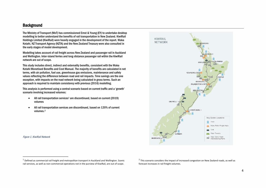
The Ministry of Transport (MoT) has commissioned Ernst & Young (EY) to undertake desktop
modelling to better understand the benefits of rail transportation in New Zealand. KiwiRail
Holdings Limited (KiwiRail) were heavily engaged in the development of the report. Waka
Kotahi, NZ Transport Agency (NZTA) and the New Zealand Treasury were also consulted in
the early stages of model development.
Modelling takes account of rail freight across New Zealand and passenger rail in Auckland
and Wellington. Inter-island ferries and long-distance passenger rail within the KiwiRail
network are out of scope.
This study includes direct, indirect and externality benefits, consistent with the Waka
Kotahi Monetised Benefits and Cost Manual. The majority of benefits are calculated in net
terms, with air pollution, fuel use, greenhouse gas emissions, maintenance and safety
values reflecting the difference between road and rail impacts. Time savings are the one
exception, with impacts on the road network being calculated in gross terms. Such an
approach is required to maintain consistency with previous (2016) modelling.
This analysis is performed using a central scenario based on current traffic and a ‘growth’
scenario involving increased volumes:
• All rail transportation services1 are discontinued, based on current (2019)
volumes
• All rail transportation services are discontinued, based on 120% of current
volumes.2
Figure 1. KiwiRail Network
1 Defined as commercial rail freight and metropolitan transport in Auckland and Wellington. Scenic
rail services, as well as non-commercial operations not in the purview of KiwiRail, are out of scope.
2 This scenario considers the impact of increased congestion on New Zealand roads, as well as
forecast increases in rail freight volumes.
5
Values are estimated by measuring the impact of shifting all rail services to road. Four
categories of benefit were examined in the 2016 Value of Rail modelling, based on
discussions with stakeholders and industry representatives.
This report includes an additional two benefit categories, taking advantage of new research
published by Waka Kotahi, NZTA, MoT and Ministry for the Environment (MfE). The six
impacts consist of:
• Road congestion (including value of time)
• Greenhouse gas emissions
• Safety
• Maintenance
• New: Fuel savings
• New: Air pollution (NOx, PM10, PM2.5 and SOx).3
For several of these impacts, sensitivity analysis has been performed to identify the impact
of alternative assumptions. For example if road congestion was limited to the ‘increment’
specified in NZTA guidance, or if traffic modelling results were not updated for historic
growth.
What this modelling is and what it is not
This study is not a full business case or economic forecasting model. While the
methodology is consistent with economic appraisal guidance, it does not attempt to
capture all the strategic, financial, commercial and infrastructure-management
implications of discontinuing rail services in New Zealand. Rail travel (freight and
passenger) provides a wider range of value to New Zealand economy than what is captured
through this analysis, for example:
• Economic Impacts: The stimulus and employment effects of the rail industry on
output (GDP).
• Opportunity cost avoided (capex): It is unlikely that the New Zealand state
highway network could absorb an increase in road vehicle tonne kilometres
(TKMs) of almost 20% without significant additional investment.
3 Nitrogen oxide, particulate matter and sulphur oxides. 4 Freight volumes were transferred onto hypothetical truck movements and passenger boardings
were transferred to a combination of private vehicles and other public transport.
• Cost to serve differentials: Current rail freight services are being purchased by
private firms because they are less expensive than alternative mode choices. For
many industries, rail supports a more cost-effective supply chain.
2016 Value of Rail model
In 2016, EY developed a comparative, static economic model (the 2016 Value of Rail
model), used to estimate the value of freight and passenger rail services in New Zealand.
The model explored a scenario where rail services did not exist, and contemporary freight
and passenger volumes were shifted to road.4 Outputs work were subsequently published
online.5
2020 Value of Rail methodology
The 2020 study applies the same conceptual approach as 2016 modelling, estimating the
impact on New Zealand if freight and passenger rail services were to be discontinued.
As noted on page 4 above, both studies include direct, indirect and externality benefits.
Modelling has been updated to reflect recent rail traffic volumes, additional benefit
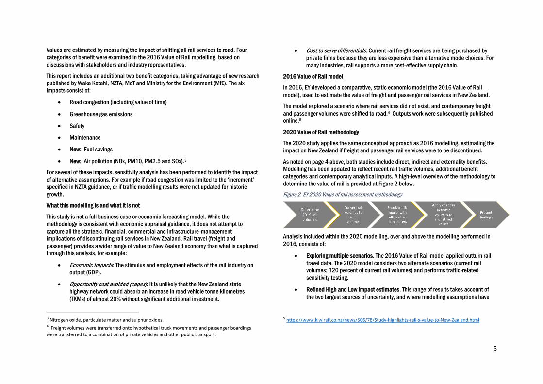
categories and contemporary analytical inputs. A high-level overview of the methodology to
determine the value of rail is provided at Figure 2 below.
Figure 2. EY 2020 Value of rail assessment methodology
Analysis included within the 2020 modelling, over and above the modelling performed in
2016, consists of:
• Exploring multiple scenarios. The 2016 Value of Rail model applied outturn rail
travel data. The 2020 model considers two alternate scenarios (current rail
volumes; 120 percent of current rail volumes) and performs traffic-related
sensitivity testing.
• Refined High and Low impact estimates. This range of results takes account of
the two largest sources of uncertainty, and where modelling assumptions have
5 https://www.kiwirail.co.nz/news/506/78/Study-highlights-rail-s-value-to-New-Zealand.html
6
the largest impact, namely the inclusion of metro road traffic uplift when
calculating congestion benefits, and the choice of input data for air pollution
(NOx) calculations. These are detailed on pages 20 and 23 respectively.
• Presentation of aggregate data. The 2016 Value of Rail model considered a line
by line assessment of value, whereas the 2020 modelling considers wider
impacts in aggregate (i.e. total net tonne-kilometres, or NTKs, vs line by line
NTKs).
• Updates to monetisation values. Contemporary research, guidance and statistics
have been drawn upon. These include updates to core input data (such as the
value of time in the EEM)6 as well as updated assumptions (such as
measurement of carbon dioxide equivalent emissions by MfE). References are
provided in footnotes throughout the report.
• Refinement of traffic modelling parameters. A range of amendments to the
modelling have been made to improve the accuracy of results.
• Presentation of benefits as they accrue to heavy and light vehicles. Rather than
presenting benefits as they accrue from rail passenger and rail freight uses,
modelling is based on vehicle types and associated impacts.
The remainder of this report outlines the results of analysis (Chapter 2), describes the
technical specifications of the modelling and explains the core assumptions underpinning
each stage of reporting (Chapter 3).
Annex 1 provides a methodology for the consideration of an augmented base case. Annex 2
provides a comparison to the 2016 Value of Rail work. Annex 3 and Annex 4 then provide
the technical specifications of the transport modelling undertaken in Wellington and
Auckland respectively.
6 The Waka Kotahi Economic Evaluation Manual was the latest guidance available when modelling
was performed.
7
2
Findings
8
Findings
The following chapter presents the findings of the value of rail modelling.
First, the core findings of the value of rail modelling are presented through monetised
estimates. Results are presented in the form of a low - high range in order to convey the
implications of alternative traffic growth and air pollution assumptions:
• Low Impact: Traffic modelling outputs are scaled for passenger rail growth in
Auckland and Wellington (c. 25%). National emissions estimates, published by
MBIE, are used to calculate nitrogen oxide impacts.
• High Impact: Traffic modelling outputs are scaled for rail and road traffic growth
in Auckland and Wellington (c. 40% - 50%). Ministry for the Environment (MfE)
emissions guidance is used to calculate nitrogen oxide impacts.
Second, the implications of a 20% uplift in rail volume are presented. These results are
provided to demonstrate how impacts could be expected to change over time and indicate
the sensitivity of different types of benefit to volume growth.
Third, mode-shift related sensitivities are presented. Truck conversion factors, 7 for
example, influence the outcome of modelling. An alternative results table is included to
communicate the impact of an alternative assumption.
Fourth, sensitivities related to traffic modelling are outlined. This identifies the impact of
assumptions related to historic travel growth. It also notes the effect of calculating the cost
of congestion using the marginal cost of congestion, as opposed to the full value of time,
which provides an indication of net congestion impacts in Auckland and Wellington.
Finally, a short comparison to the 2016 Value of Rail modelling is included to demonstrate
the dynamic nature of this modelling and provide a reference point to the original work.
Core findings
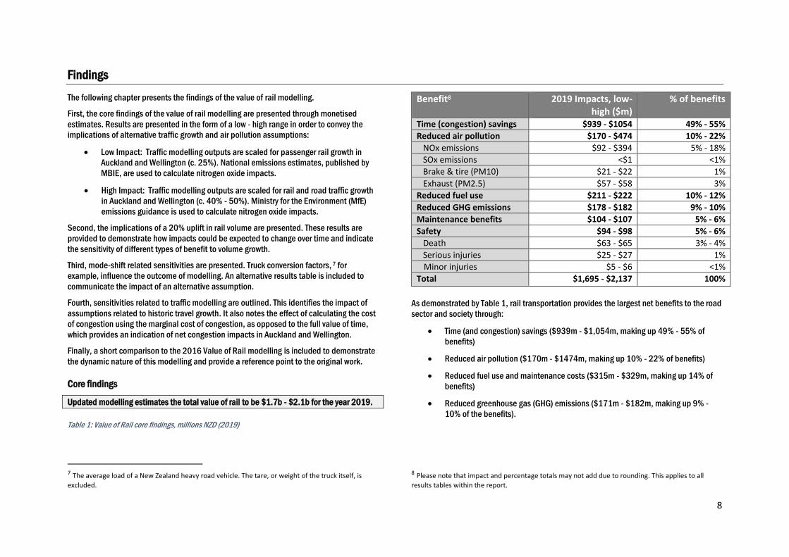
Updated modelling estimates the total value of rail to be $1.7b - $2.1b for the year 2019.
Table 1: Value of Rail core findings, millions NZD (2019)
7 The average load of a New Zealand heavy road vehicle. The tare, or weight of the truck itself, is
excluded.
Benefit8 2019 Impacts, low-high ($m)
% of benefits
Time (congestion) savings $939 - $1054 49% - 55%
Reduced air pollution $170 - $474 10% - 22%
NOx emissions $92 - $394 5% - 18%
SOx emissions <$1 <1%
Brake & tire (PM10) $21 - $22 1%
Exhaust (PM2.5) $57 - $58 3%
Reduced fuel use $211 - $222 10% - 12%
Reduced GHG emissions $178 - $182 9% - 10%
Maintenance benefits $104 - $107 5% - 6%
Safety $94 - $98 5% - 6%
Death $63 - $65 3% - 4%
Serious injuries $25 - $27 1%
Minor injuries $5 - $6 <1%
Total $1,695 - $2,137 100%
As demonstrated by Table 1, rail transportation provides the largest net benefits to the road
sector and society through:
• Time (and congestion) savings ($939m - $1,054m, making up 49% - 55% of
benefits)
• Reduced air pollution ($170m - $1474m, making up 10% - 22% of benefits)
• Reduced fuel use and maintenance costs ($315m - $329m, making up 14% of
benefits)
• Reduced greenhouse gas (GHG) emissions ($171m - $182m, making up 9% -
10% of the benefits).
8 Please note that impact and percentage totals may not add due to rounding. This applies to all
results tables within the report.
9
A summary of the monetisation factors underpinning calculations is provided in Table 2.
Further detail about the sources for these calculations, as well as the underlying
methodology, is provided in Chapter 3.
Table 2: Monetisation values and conversion factors for core findings
Benefit Value (2019 dollars) Truck conversion factor 9.6t (rail NTKs to road KMs)
Time (congestion) savings9
Morning commuter peak $29.50 / hour
Daytime interpeak peak $27.64 / hour
Afternoon commuter peak $28.46 / hour
Safety Average of 4 years
Death $4,470,200 per death
Serious injury $472,152 per injury
Minor injury $25,441 per injury
Reduced GHG emissions $71.50 / tonne CO2-e
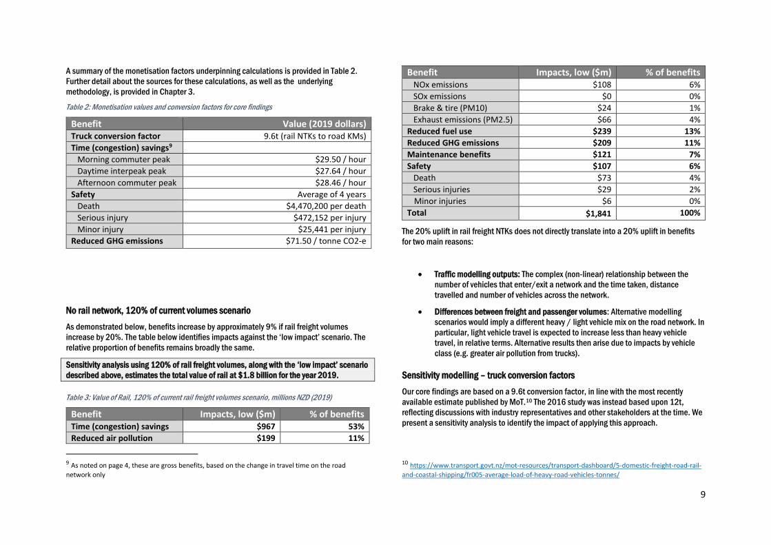
No rail network, 120% of current volumes scenario
As demonstrated below, benefits increase by approximately 9% if rail freight volumes
increase by 20%. The table below identifies impacts against the ‘low impact’ scenario. The
relative proportion of benefits remains broadly the same.
Sensitivity analysis using 120% of rail freight volumes, along with the ‘low impact’ scenario
described above, estimates the total value of rail at $1.8 billion for the year 2019.
Table 3: Value of Rail, 120% of current rail freight volumes scenario, millions NZD (2019)
Benefit Impacts, low ($m) % of benefits Time (congestion) savings $967 53%
Reduced air pollution $199 11%
9 As noted on page 4, these are gross benefits, based on the change in travel time on the road
network only
Benefit Impacts, low ($m) % of benefits NOx emissions $108 6%
SOx emissions $0 0%
Brake & tire (PM10) $24 1%
Exhaust emissions (PM2.5) $66 4%
Reduced fuel use $239 13%
Reduced GHG emissions $209 11%
Maintenance benefits $121 7%
Safety $107 6%
Death $73 4%
Serious injuries $29 2%
Minor injuries $6 0%
Total $1,841 100%
The 20% uplift in rail freight NTKs does not directly translate into a 20% uplift in benefits
for two main reasons:
• Traffic modelling outputs: The complex (non-linear) relationship between the
number of vehicles that enter/exit a network and the time taken, distance
travelled and number of vehicles across the network.
• Differences between freight and passenger volumes: Alternative modelling
scenarios would imply a different heavy / light vehicle mix on the road network. In
particular, light vehicle travel is expected to increase less than heavy vehicle
travel, in relative terms. Alternative results then arise due to impacts by vehicle
class (e.g. greater air pollution from trucks).
Sensitivity modelling – truck conversion factors
Our core findings are based on a 9.6t conversion factor, in line with the most recently
available estimate published by MoT.10 The 2016 study was instead based upon 12t,
reflecting discussions with industry representatives and other stakeholders at the time. We
present a sensitivity analysis to identify the impact of applying this approach.
10 https://www.transport.govt.nz/mot-resources/transport-dashboard/5-domestic-freight-road-rail-
and-coastal-shipping/fr005-average-load-of-heavy-road-vehicles-tonnes/
10
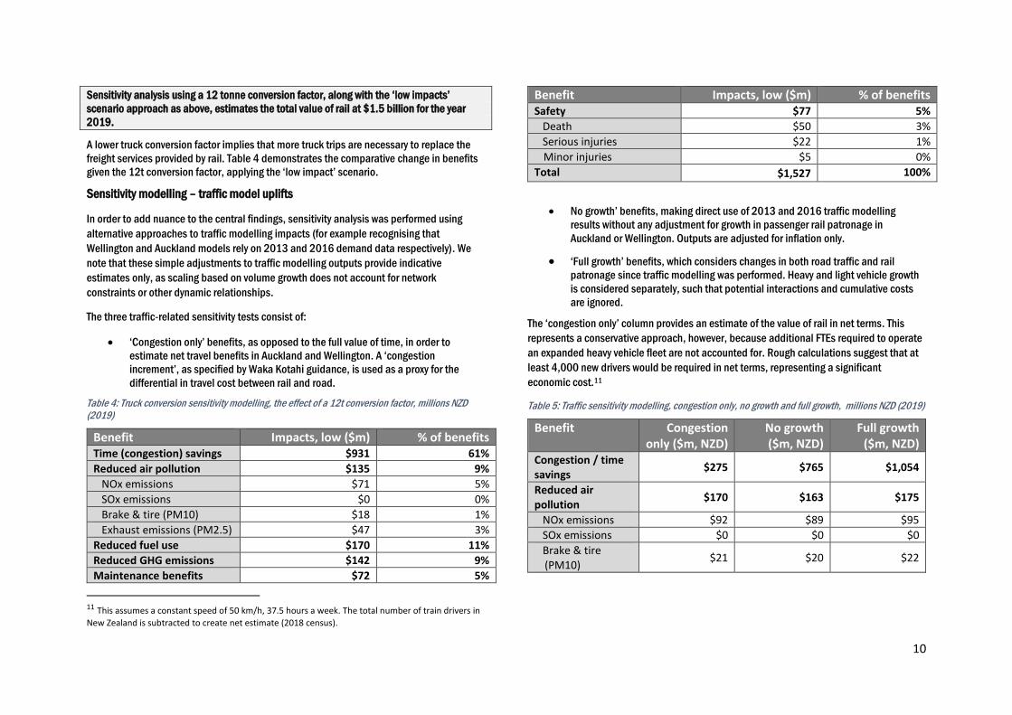
Sensitivity analysis using a 12 tonne conversion factor, along with the ‘low impacts’
scenario approach as above, estimates the total value of rail at $1.5 billion for the year
2019.
A lower truck conversion factor implies that more truck trips are necessary to replace the
freight services provided by rail. Table 4 demonstrates the comparative change in benefits
given the 12t conversion factor, applying the ‘low impact’ scenario.
Sensitivity modelling – traffic model uplifts
In order to add nuance to the central findings, sensitivity analysis was performed using
alternative approaches to traffic modelling impacts (for example recognising that
Wellington and Auckland models rely on 2013 and 2016 demand data respectively). We
note that these simple adjustments to traffic modelling outputs provide indicative
estimates only, as scaling based on volume growth does not account for network
constraints or other dynamic relationships.
The three traffic-related sensitivity tests consist of:
• ‘Congestion only’ benefits, as opposed to the full value of time, in order to
estimate net travel benefits in Auckland and Wellington. A ‘congestion
increment’, as specified by Waka Kotahi guidance, is used as a proxy for the
differential in travel cost between rail and road.
Table 4: Truck conversion sensitivity modelling, the effect of a 12t conversion factor, millions NZD (2019)
Benefit Impacts, low ($m) % of benefits Time (congestion) savings $931 61%
Reduced air pollution $135 9%
NOx emissions $71 5%
SOx emissions $0 0%
Brake & tire (PM10) $18 1%
Exhaust emissions (PM2.5) $47 3%
Reduced fuel use $170 11%
Reduced GHG emissions $142 9%
Maintenance benefits $72 5%
11 This assumes a constant speed of 50 km/h, 37.5 hours a week. The total number of train drivers in
New Zealand is subtracted to create net estimate (2018 census).
Benefit Impacts, low ($m) % of benefits Safety $77 5%
Death $50 3%
Serious injuries $22 1%
Minor injuries $5 0%
Total $1,527 100%
• No growth’ benefits, making direct use of 2013 and 2016 traffic modelling
results without any adjustment for growth in passenger rail patronage in
Auckland or Wellington. Outputs are adjusted for inflation only.
• ‘Full growth’ benefits, which considers changes in both road traffic and rail
patronage since traffic modelling was performed. Heavy and light vehicle growth
is considered separately, such that potential interactions and cumulative costs
are ignored.
The ‘congestion only’ column provides an estimate of the value of rail in net terms. This
represents a conservative approach, however, because additional FTEs required to operate
an expanded heavy vehicle fleet are not accounted for. Rough calculations suggest that at
least 4,000 new drivers would be required in net terms, representing a significant
economic cost.11
Table 5: Traffic sensitivity modelling, congestion only, no growth and full growth, millions NZD (2019)
Benefit Congestion only ($m, NZD)
No growth ($m, NZD)
Full growth ($m, NZD)
Congestion / time savings
$275 $765 $1,054
Reduced air pollution
$170 $163 $175
NOx emissions $92 $89 $95
SOx emissions $0 $0 $0
Brake & tire (PM10)
$21 $20 $22
11
Benefit Congestion only ($m, NZD)
No growth ($m, NZD)
Full growth ($m, NZD)
Exhaust emissions (PM2.5)
$57 $54 $58
Reduced fuel use $211 $194 $222
Reduced GHG emissions
$178 $171 $182
Maintenance benefits
$104 $98 $107
Safety $94 $87 $98
Death $63 $59 $65
Serious injuries $25 $23 $27
Minor injuries $5 $5 $6
Total $1,031 $1,478 $1,837
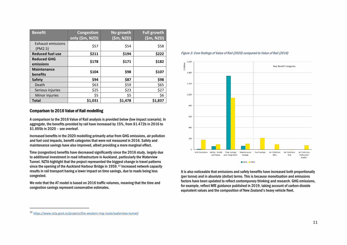
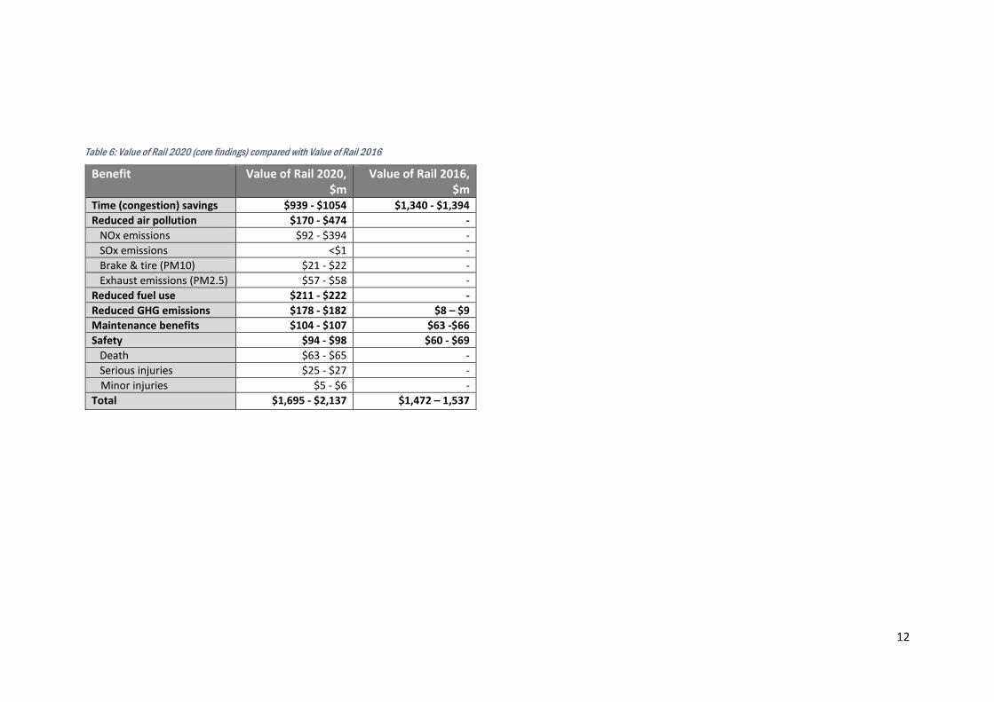
Comparison to 2016 Value of Rail modelling
A comparison to the 2016 Value of Rail analysis is provided below (low impact scenario). In
aggregate, the benefits provided by rail have increased by 15%, from $1.472b in 2016 to
$1.695b in 2020 – see overleaf.
Increased benefits in the 2020 modelling primarily arise from GHG emissions, air pollution
and fuel cost impacts, benefit categories that were not measured in 2016. Safety and
maintenance savings have also improved, albeit providing a more marginal effect.
Time (congestion) benefits have decreased significantly since the 2016 study, largely due
to additional investment in road infrastructure in Auckland, particularly the Waterview
Tunnel. NZTA highlight that the project represented the biggest change in travel patterns
since the opening of the Auckland Harbour Bridge in 1959.12 Increased network capacity
results in rail transport having a lower impact on time savings, due to roads being less
congested.
We note that the AT model is based on 2016 traffic volumes, meaning that the time and
congestion savings represent conservative estimates.
12 https://www.nzta.govt.nz/projects/the-western-ring-route/waterview-tunnel/
Figure 3: Core findings of Value of Rail (2020) compared to Value of Rail (2016)
It is also noticeable that emissions and safety benefits have increased both proportionally
(per tonne) and in absolute (dollar) terms. This is because monetisation and emissions
factors have been updated to reflect contemporary thinking and research. GHG emissions,
for example, reflect MfE guidance published in 2019, taking account of carbon dioxide
equivalent values and the composition of New Zealand’s heavy vehicle fleet.
12
Table 6: Value of Rail 2020 (core findings) compared with Value of Rail 2016
Benefit Value of Rail 2020, $m
Value of Rail 2016, $m
Time (congestion) savings $939 - $1054 $1,340 - $1,394
Reduced air pollution $170 - $474 -
NOx emissions $92 - $394 -
SOx emissions <$1 -
Brake & tire (PM10) $21 - $22 -
Exhaust emissions (PM2.5) $57 - $58 -
Reduced fuel use $211 - $222 -
Reduced GHG emissions $178 - $182 $8 – $9
Maintenance benefits $104 - $107 $63 -$66
Safety $94 - $98 $60 - $69
Death $63 - $65 -
Serious injuries $25 - $27 -
Minor injuries $5 - $6 -
Total $1,695 - $2,137 $1,472 – 1,537
13
3
Methodology
14
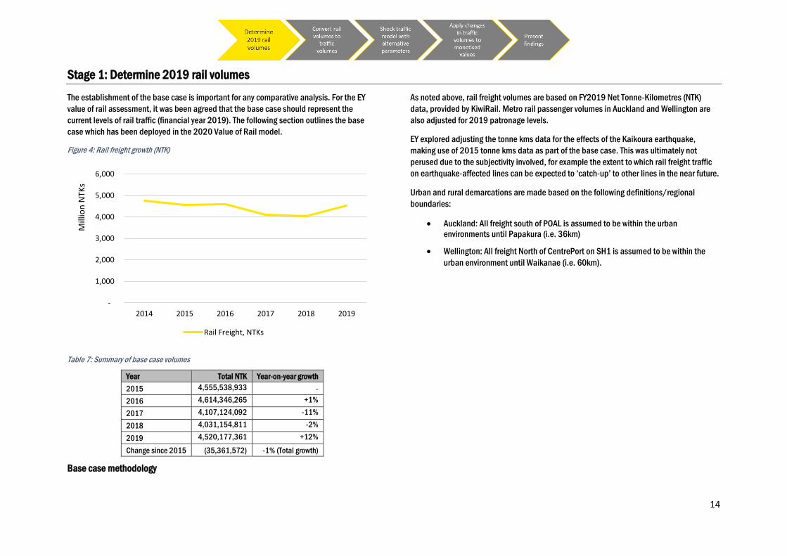
Stage 1: Determine 2019 rail volumes
The establishment of the base case is important for any comparative analysis. For the EY
value of rail assessment, it was been agreed that the base case should represent the
current levels of rail traffic (financial year 2019). The following section outlines the base
case which has been deployed in the 2020 Value of Rail model.
Figure 4: Rail freight growth (NTK)
Table 7: Summary of base case volumes
Year Total NTK Year-on-year growth
2015 4,555,538,933 -
2016 4,614,346,265 +1%
2017 4,107,124,092 -11%
2018 4,031,154,811 -2%
2019 4,520,177,361 +12%
Change since 2015 (35,361,572) -1% (Total growth)
Base case methodology
As noted above, rail freight volumes are based on FY2019 Net Tonne-Kilometres (NTK)
data, provided by KiwiRail. Metro rail passenger volumes in Auckland and Wellington are
also adjusted for 2019 patronage levels.
EY explored adjusting the tonne kms data for the effects of the Kaikoura earthquake,
making use of 2015 tonne kms data as part of the base case. This was ultimately not
perused due to the subjectivity involved, for example the extent to which rail freight traffic
on earthquake-affected lines can be expected to ‘catch-up’ to other lines in the near future.
Urban and rural demarcations are made based on the following definitions/regional
boundaries:
• Auckland: All freight south of POAL is assumed to be within the urban
environments until Papakura (i.e. 36km)
• Wellington: All freight North of CentrePort on SH1 is assumed to be within the
urban environment until Waikanae (i.e. 60km).
-
1,000
2,000
3,000
4,000
5,000
6,000
2014 2015 2016 2017 2018 2019
Mill
ion
NTK
s
Rail Freight, NTKs
15
Stage 2: Convert rail volumes to road travel volumes
There are two steps involved in Stage 2:
• The determination of relevant freight volume scenarios
• Converting rail volumes into commensurate traffic volumes.
Determination of relevant scenarios
A range of scenarios were originally considered as part of this package of work ranging from
managed decline through to significant investment in the rail network.
Eventually, a decision was reached to test two key scenarios:
1. No rail network, current (2019) freight and passenger volumes
Assumes that all freight and passenger travel currently provided through rail is shifted to
the road network. As explained in Stage 1, base case volumes involve 2019 outturn data.
This is effectively a ‘re-run’ of the 2016 Value of Rail work completed by EY.
2. No rail network, 120 percent of freight volumes
Freight: Applies a 20 percent uplift to 2019 outturn freight volumes. This is a realistic
projection for medium-term industry growth and aligns with the Ministry of Transport’s
report “Transport Outlook: Future State”. This report suggests that a 20% increase in freight
volumes would be achieved by approximately 2027/28.
As all input data is based on pre-2020 activity, modelling does not reflect the impacts of
COVID-19.
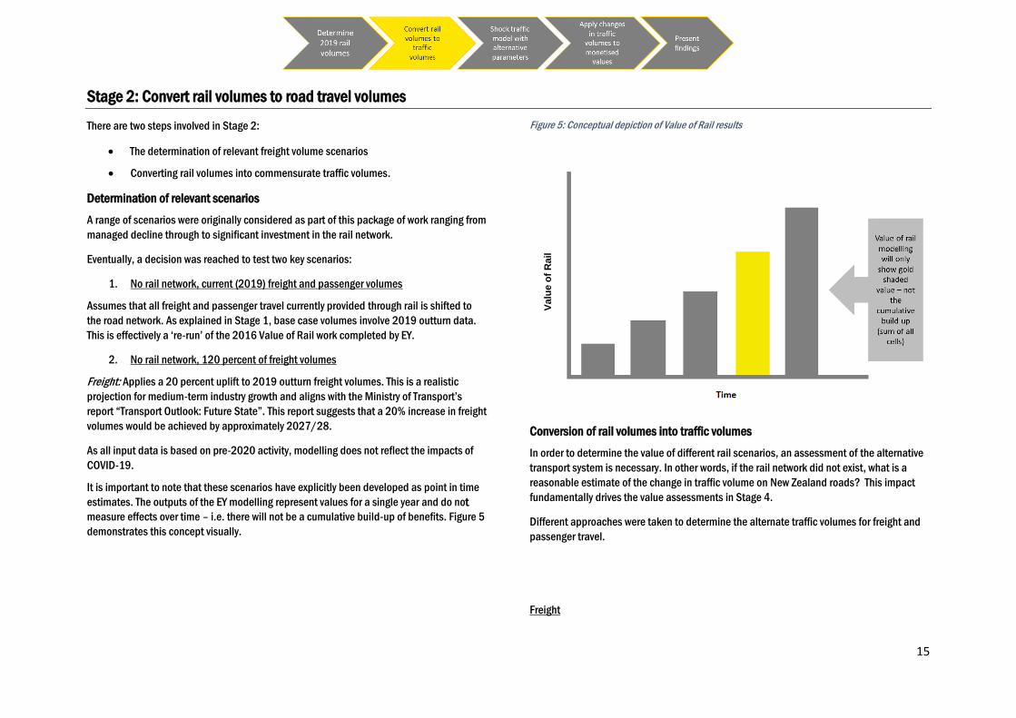
It is important to note that these scenarios have explicitly been developed as point in time
estimates. The outputs of the EY modelling represent values for a single year and do not
measure effects over time – i.e. there will not be a cumulative build-up of benefits. Figure 5
demonstrates this concept visually.
Figure 5: Conceptual depiction of Value of Rail results
Conversion of rail volumes into traffic volumes
In order to determine the value of different rail scenarios, an assessment of the alternative
transport system is necessary. In other words, if the rail network did not exist, what is a
reasonable estimate of the change in traffic volume on New Zealand roads? This impact
fundamentally drives the value assessments in Stage 4.
Different approaches were taken to determine the alternate traffic volumes for freight and
passenger travel.
Freight
Valu
e o
f R
ail
16
A conversion factor of 9.6 tonnes per truck was deployed for this analysis, making use of
published MoT data. 13 That being, every 9.6 tonnes of freight volume carried on the rail
network equates to one additional truck on the road. Given that rail freight volumes are
reported in Net Tonne-Kilometres (NTKs), 14 traffic was adjusted for the comparative length
of travel of each journey to calculate equivalent road kilometres travelled.
Modelling assumes that all new trucks on the road consistently carry 9.6 tonnes and does
not attempt to adjust for empty return trips, beyond what is already in the national average.
Findings therefore represent a conservative value if an absence of rail freight would
increase the proportion of ‘empty’ road journeys.
For the sensitivity analysis, a 12t truck conversion factor was employed. This is consistent
with the conversion factor used from Value of Rail 2016. The following table highlights the
change in truck trips under each scenario, before any uplifts for metro growth are applied.
Table 8: Daily trucks to be removed/added for the transport modelling
Scenario Auckland Wellington
No rail network, current
volumes 781 increase 298 increase
No rail network, 120%
of volumes
156 increase
(additional)
60 increase
(additional)
We note that the ‘120% of current volumes’ row was originally calculated in reverse, such
that the impact of a 20% decrease in traffic volumes was estimated. These values are
additional to the ‘no rail network’ estimate, such that the total estimated change for
Auckland and Wellington is 937 and 358 trucks respectively under the 120% scenario.
Passenger
Passenger rail conversion factors have only been applied in the Metro areas (Wellington
and Auckland) as large-scale passenger rail services do not operate outside of these cities.
These impacts are additional to the freight effects described above, and do not apply the
same ‘per tonne’ conversion factor.
The precise conversion rates have been taken from Auckland Transport (AT) and Greater
Wellington Regional Council (GWRC) transport models. These models have in-built vectors,
based on travel demand surveying, that show the different behavioural decisions of
13 https://www.transport.govt.nz/mot-resources/transport-dashboard/5-domestic-freight-road-rail-
and-coastal-shipping/fr005-average-load-of-heavy-road-vehicles-tonnes/
passengers. EY has not adjusted these assumptions throughout the conversion process,
with the exception of the sensitivities described on page 9.
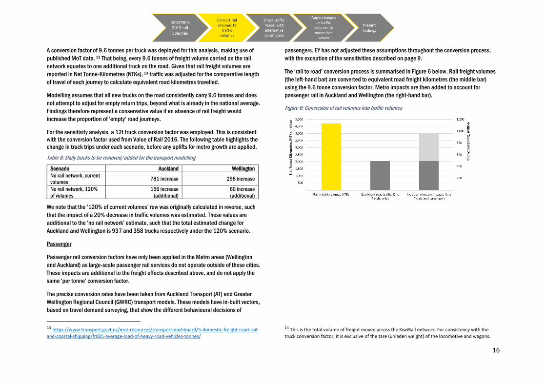
The ‘rail to road’ conversion process is summarised in Figure 6 below. Rail freight volumes
(the left-hand bar) are converted to equivalent road freight kilometres (the middle bar)
using the 9.6 tonne conversion factor. Metro impacts are then added to account for
passenger rail in Auckland and Wellington (the right-hand bar).
Figure 6: Conversion of rail volumes into traffic volumes
14 This is the total volume of freight moved across the KiwiRail network. For consistency with the
truck conversion factor, it is exclusive of the tare (unladen weight) of the locomotive and wagons.
17
Stage 3: Undertake traffic modelling
A fundamental feature of this analysis is the incorporation of transport modelling in the
metro areas (Wellington and Auckland) where rail passenger services are available. This
feature is important as it provides a level of dynamism to the modelling. That said, it adds
an additional layer of complexity to the analytical task.
Results are calculated as the difference between ‘with and without rail’ journey times and
travel distance, considering road travel only (i.e. rail travel time is not considered). A
sensitivity analysis, which seeks to estimate marginal impacts across both modes, is
described on page 10.
Total alternate truck trips/counts were established in Stage 2 and the results of these have
been fed into the traffic modelling.
Auckland Transport’s Macro Strategic Model (MSM) model and GWRC’s Wellington
Regional Strategic Model (WTSM) were employed to undertake this task. Both models have
different operating assumptions but appear to be built on the same traffic modelling
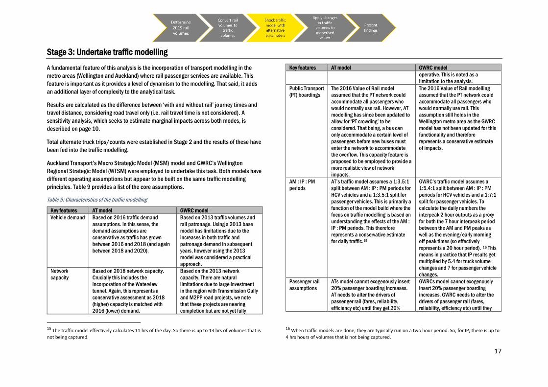
principles. Table 9 provides a list of the core assumptions.
Table 9: Characteristics of the traffic modelling
Key features AT model GWRC model
Vehicle demand Based on 2016 traffic demand
assumptions. In this sense, the
demand assumptions are
conservative as traffic has grown
between 2016 and 2018 (and again
between 2018 and 2020).
Based on 2013 traffic volumes and
rail patronage. Using a 2013 base
model has limitations due to the
increases in both traffic and
patronage demand in subsequent
years, however using the 2013
model was considered a practical
approach.
Network
capacity
Based on 2018 network capacity.
Crucially this includes the
incorporation of the Waterview
tunnel. Again, this represents a
conservative assessment as 2018
(higher) capacity is matched with
2016 (lower) demand.
Based on the 2013 network
capacity. There are natural
limitations due to large investment
in the region with Transmission Gully
and M2PP road projects, we note
that these projects are nearing
completion but are not yet fully
15 The traffic model effectively calculates 11 hrs of the day. So there is up to 13 hrs of volumes that is
not being captured.
Key features AT model GWRC model
operative. This is noted as a
limitation to the analysis.
Public Transport
(PT) boardings
The 2016 Value of Rail model
assumed that the PT network could
accommodate all passengers who
would normally use rail. However, AT
modelling has since been updated to
allow for ‘PT crowding’ to be
considered. That being, a bus can
only accommodate a certain level of
passengers before new buses must
enter the network to accommodate
the overflow. This capacity feature is
proposed to be employed to provide a
more realistic view of network
impacts.
The 2016 Value of Rail modelling
assumed that the PT network could
accommodate all passengers who
would normally use rail. This
assumption still holds in the
Wellington metro area as the GWRC
model has not been updated for this
functionality and therefore
represents a conservative estimate
of impacts.
AM : IP : PM
periods
AT’s traffic model assumes a 1:3.5:1
split between AM : IP : PM periods for
HCV vehicles and a 1:3.5:1 split for
passenger vehicles. This is primarily a
function of the model build where the
focus on traffic modelling is based on
understanding the effects of the AM :
IP : PM periods. This therefore
represents a conservative estimate
for daily traffic.15
GWRC’s traffic model assumes a
1:5.4:1 split between AM : IP : PM
periods for HCV vehicles and a 1:7:1
split for passenger vehicles. To
calculate the daily numbers the
interpeak 2 hour outputs as a proxy
for both the 7 hour interpeak period
between the AM and PM peaks as
well as the evening/early morning
off peak times (so effectively
represents a 20 hour period). 16 This
means in practice that IP results get
multiplied by 5.4 for truck volume
changes and 7 for passenger vehicle
changes.
Passenger rail
assumptions
ATs model cannot exogenously insert
20% passenger boarding increases.
AT needs to alter the drivers of
passenger rail (fares, reliability,
efficiency etc) until they get 20%
GWRCs model cannot exogenously
insert 20% passenger boarding
increases. GWRC needs to alter the
drivers of passenger rail (fares,
reliability, efficiency etc) until they
16 When traffic models are done, they are typically run on a two hour period. So, for IP, there is up to
4 hrs hours of volumes that is not being captured.
18
Key features AT model GWRC model
passenger boarding changes. In
practice this has resulted in:
• Freq rail *1.4 (Headway
*1/1.4)
• SS runtime * 0.7
(Speed/0.7)
• Rail Fare * 0.7
Figures were eventually within 19% -
21% for all travel time periods.
get 20% passenger boarding
changes. In practice this has
resulted in:
• A number of tests were
run to determine which In
Vehicle Time (IVT) factor
would lead to the desired
increase in patronage.
The IVT factor is 0.9 by
default and was changed
to 0.25 in order to
achieve a 20% increase
in patronage.
Figures that were eventually within
19% - 21% for all travel time
periods.
Yearly
conversion
A yearly conversion was undertaken
to gross up numbers from daily to
yearly. A 280 day conversion was
used to take into consideration the
weekend traffic compared to a 245
weekday. 280 is considered
conservative as it does not account
for all days of the weekend.
A yearly conversion was undertaken
to gross up numbers from daily to
yearly. A 280 day conversion was
used to take into consideration the
weekend traffic compared to a 245
weekday. 280 is considered
conservative as it does not account
for all days of the weekend.
Traffic volumes provided
As noted above, changes in truck trips/counts associated with each scenario were derived
by EY in Stage 2 and provided direct to AT and GWRC to determine changes in traffic
volumes. Changes in passenger counts associated with changes in passenger volumes
have been determined endogenously by GWRC and AT models.
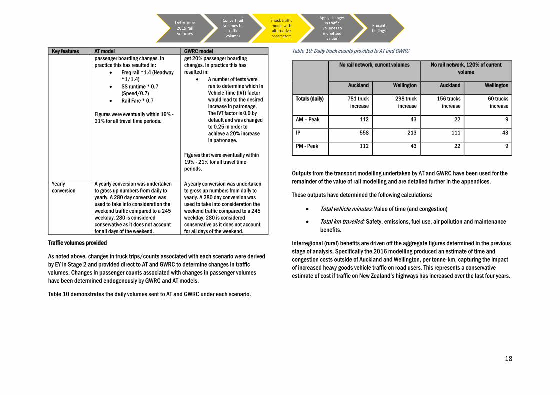
Table 10 demonstrates the daily volumes sent to AT and GWRC under each scenario.
Table 10: Daily truck counts provided to AT and GWRC
Outputs from the transport modelling undertaken by AT and GWRC have been used for the
remainder of the value of rail modelling and are detailed further in the appendices.
These outputs have determined the following calculations:
• Total vehicle minutes: Value of time (and congestion)
• Total km travelled: Safety, emissions, fuel use, air pollution and maintenance
benefits.
Interregional (rural) benefits are driven off the aggregate figures determined in the previous
stage of analysis. Specifically the 2016 modelling produced an estimate of time and
congestion costs outside of Auckland and Wellington, per tonne-km, capturing the impact
of increased heavy goods vehicle traffic on road users. This represents a conservative
estimate of cost if traffic on New Zealand’s highways has increased over the last four years.
No rail network, current volumes No rail network, 120% of current
volume
Auckland Wellington Auckland Wellington
Totals (daily) 781 truck
increase
298 truck
increase
156 trucks
increase
60 trucks
increase
AM – Peak 112 43 22 9
IP 558 213 111 43
PM - Peak 112 43 22 9
19
Step 4: Undertake impact assessment
Impact assessment is based on a marginal change in traffic volume, applying metrics such
as vehicle counts and travel time. This valuation process uses well-established economic
values, as well as sensitivity tests where appropriate, to provide a reasonable indication of
the value of rail under different investment scenarios.
An important feature of this modelling is the calculation of gross and net benefits (or
disbenefits):
• Gross benefits are those that result from an increase or decrease in road traffic
only under a given scenario. For example, the GHG emissions avoided if heavy
vehicle travel is reduced.
• Net benefits also encompass the rail impacts of a given scenario. For example,
the GHG avoided if heavy vehicle travel is reduced, minus the GHG emissions
associated with rail transportation.
Each benefit category is explained below, including the approach to monetisation
(converting impacts to dollar terms). To aid communication, relevant volume drivers are
reiterated under each heading. A summary of the core assumptions used in the modelling
is then provided at the conclusion of each section.
Value of congestion
Volume drivers
• Urban: Changes in time taken to complete road travel have been employed as the
input variable that drives this assessment. This has been taken from the traffic
modelling undertaken by AT and GWRC respectively.
• Rural: The volume driver for this has been total NTKs less the metro NTKs.
As traffic modelling is based on historic levels of demand (2013 and 2016 for Wellington
and Auckland respectively), outputs are adjusted for volume growth over the last 3-6 years
in these metro areas. The ‘low impact’ scenario takes account of passenger rail growth
only, whereas the ‘high impact’ scenario includes road and rail traffic growth.
In both cases, traffic model impacts are multiplied by volume increases, such that dynamic
and / or cumulative interactions are not considered. This represents a conservative
approach in light of road network capacity limitations.
Monetisation values
The value of time metrics included in the EEM have been used to determine time and
congestion benefits. The latter is applied to morning and afternoon peak times only.
Different value of time proxies have been assumed for metro and interregional benefits.
These figures are consistent with best practice in transport evaluation.
Specifically:
• Urban: The value of time (congestion) has been derived from the values of time
listed under table A4.3 in the EEM, adjusted for inflation. In essence the AM: IP:
PM: traffic counts align to the commensurate base value of time metric as per
below. As noted above, the increment for congestion is applied at morning and
afternoon peak times only.
• Rural: The total lower bound interregional freight benefit from the 2016 Value of
Rail report divided by the total tonne kms of the 2016 Value of Rail report has
been employed to derive a benefit per tonne km. The average rural benefit is
calculated at $0.028 per tonne km removed.
This approach is considered appropriate because of the aggregate nature of the 2020
analysis. In 2016, a line-by-line assessment was undertaken which meant that vehicle flow
rates could be determined for each road, and hence the marginal impacts of changes in rail
across different roads could be estimated. By definition, this calculation is not possible at
an aggregate level. Accordingly, an ‘average’ of the 2016 estimate is applied.
Consideration was given to using different value of time metrics prescribed by the EEM,
notably trip purpose. This was not progressed, however, as it would require additional
assumptions to be made about the general purpose of AM: IP: PM: travel.
20
Update factors were applied to all values to account inflation.17 In particular, travel time
cost savings, crash cost savings and emission reduction benefits. 2019 prices have been
applied across the board, making use of published update factors wherever possible.
Net congestion figures
As noted on page 16, value of congestion in this study examines the ‘with vs. without rail’
impacts on road travel in Auckland and Wellington. It does not take account of travel time
impacts on other modes, for example passenger rail travel, and is therefore measured in
gross terms. A sensitivity analysis, exploring the impact of an alternative methodology, can
be found on pages 10-11.
The off-setting congestion impact on the rail network is not be considered within this
assessment. This is because metro rail in New Zealand is not yet facing the same capacity
constraints as urban roads.
Summary
Values (NZD, 2019)
Morning Commuter peak $29.28 / hour
Daytime Inter peak $27.64 / hour
Afternoon Commuter Peak $28.46 / hour
Rural $0.029 per tonne km
Greenhouse Gas Emissions
Volume drivers
• Urban: Changes in vehicle kilometres travelled have been employed as the input
variable that drives this assessment in metro areas. This has been directly taken
from the traffic modelling undertaken by AT and GWRC.
17 https://www.nzta.govt.nz/assets/resources/econoic-evaluation-manual/economic-evaluation-
manual/docs/eem-update-factors.pdf 18 https://www.mfe.govt.nz/sites/default/files/media/Climate%20Change/2019-detailed-guide.pdf
• Rural: The volume driver for interregional traffic has been total new NTKs less the
metro NTKs.
An average km per tonne proxy has then been derived to undertake this assessment, based
on guidance published by MfE.18 Published emissions factors for small trucks (table 41)
are adjusted to reflect the difference in truck size (table 45), as well as the proportional
NTKs specified in the Vehicle Emissions Prediction Model (VEPM).19
Monetisation values
The value for emissions benefits are sourced from the NZTA EEM ($71.50 per tonne of CO2-
e in 2019 dollars). Urban and rural volumes are considered interchangeably for this
assessment.
Net emission values
MfE guidance provides emissions factors for both rail and road freight, permitting an
estimate of the difference between modes. The volume calculations described above
produce an average emissions per tonne km figure for both modes. The net result
represents the GHG emissions created by additional road freight, minus the emissions
currently created by rail freight. This is equivalent to almost 2.5m tonnes of CO2-e per year.
Summary
The value of GHG emissions used in the analysis, as recommended by the EEM, is provided
below.
Values (NZD, 2019)
CO2-e, per tonne $71.50
Safety
19 https://www.nzta.govt.nz/roads-and-rail/highways-information-portal/technical-disciplines/air-
quality-climate/planning-and-assessment/vehicle-emissions-prediction-model/
21
Volume drivers
• Urban: Changes in vehicle kilometres travelled have been employed as the input
variable that drives this assessment in metro areas. This has been directly taken
from the traffic modelling undertaken by AT and GWRC.
• Rural: The volume driver for interregional traffic has been total NTKs less the
metro NTKs.
A death, serious and minor injury per km/NTK was derived from the NZTA Crash Analysis
System (CAS). A death, serious and minor per km/NTK was calculated by taking the total
yearly deaths, serious and minor injury divided by the total kms/NTK travelled. A road
freight equivalent factor was established by taking deaths, serious and minor injuries
involving trucks divided by the total kms/NTK travelled.
An average of four-year incident counts were undertaken to smooth out any outliers and/or
year to year fluctuations for the lower bound.
Monetisation values
Safety benefits have been derived from well-understood proxies of the value of life and
injury.20 These statistical values are widely utilised in transport project appraisals:
• The value of an avoided death: $4,470,200
• The value of an avoided serious injury: $472,152
• The value of an avoided minor injury: $25,441.
Net safety values
Impacts are based on an estimate of additional safety incidents per NTK, were rail services
to be replaced by road transport. An average incident per km / tonne-km was derived for
rail, light vehicles and heavy vehicles, based on total incidents divided by traffic.
20 https://www.transport.govt.nz/assets/Uploads/Research/Documents/a5f9a063d1/Social-cost-of-
road-crashes-and-injuries-2017-update-FINAL.PDF
Net results represent the death and injuries likely to be created by additional trucks and
cars on the road, minus the incidents currently caused by rail. This results in 14 avoided
deaths, 53 avoided serious injuries, and 210 avoided minor injuries.
Summary
Values (NZD, 2019)
Value of avoided deaths $4,470,200
Value of avoided serious injuries $472,152
Value of avoided minor injuries $25,441
Air Pollution
A similar approach to that of Greenhouse Gas Emissions is applied to calculate wider air
pollution impacts. Nitrous oxide (NOx), Sulphur oxide (SOx), and Particulate Matter (PMx)
all have well-established effects on human health, and thus are included in transport cost
appraisal.
Volume drivers
• Urban: Changes in vehicle kilometres travelled have been employed as the input
variable that drives this assessment in metro areas. This has been directly taken
from the traffic modelling undertaken by AT and GWRC.
• Rural: The volume driver for interregional traffic has been total NTKs less the
metro NTKs.
Multiple estimates of emissions factors have been published in recent years, and no single
study provides a comprehensive assessment of air pollution across relevent modes and
vehicle classes in New Zealand.
Road-related emissions are thoroughly explored in the NZTA Vehicle Emissions Prediction
Model (VEPM)21, but this analysis does not extend to rail. MfE research22 compares road
and rail emissions directly, but requires the use of nitrous oxide (a gas that primarily causes
21 https://www.nzta.govt.nz/roads-and-rail/highways-information-portal/technical-disciplines/air-
quality-climate/planning-and-assessment/vehicle-emissions-prediction-model/ 22 https://www.mfe.govt.nz/sites/default/files/media/Climate%20Change/2019-detailed-guide.pdf
22
damage through greenhouse effects, rather than to human health directly) as a proxy for
ratios of nitrogen oxide emissions.23
This creates challenges for accurately estimating the differentials in air pollution across
road and rail transport. NOx represents the largest source of uncertainty, as alternative
modelling assumptions have a large impact on benefit results.
MfE-based estimates of road freight NOx emissions are roughly three times larger than
VEPM-based estimates, with annual, national energy sector estimates published by MBIE24
falling in between the two.
To take account of this issue, two different methodologies have been explored:
• The ‘low impact’ scenario applies a combination of NZTA and MBIE (national,
annual energy sector emissions) modelling. This directly measures nitrogen
oxides, as defined in the EEM, but requires an amalgamation of two different
data sources.
• The ‘high impact’ scenario applies MfE research, comparing the emissions
factors associated with rail and road freight. New truck routes, in the absence of
rail, are assumed to involve a mix of urban and long-haul delivery. This approach
makes use of a single study, but measures a different chemical compound to that
recommended in the EEM.
Sulphur oxide (SOx) emissions make an insignificant impact on the value of rail regardless
of the methodology applied (i.e. less than $1 million), so MfE calorific-based emission
factors have been applied to both the high and low scenario.
Values
Monetising the health costs associated with air pollution is performed according to the
EEM. Specifically, a ‘damage cost approach’ is applied in light of the national scale of rail
freight transport:
23 MfE emissions factors are measured in carbon-dioxide equivalent units (CO2-e), however the
conversion between N2O and CO2-e (298) is very similar to the ratio of NOX to N2O road emissions in NZ according to MBIE (293), such that these two effects cancel out. 24 https://www.mbie.govt.nz/building-and-energy/energy-and-natural-resources/energy-statistics-
and-modelling/energy-statistics/new-zealand-energy-sector-greenhouse-gas-emissions/
“The damage cost approach is much simpler than undertaking exposure modelling, which requires detailed understanding of the sources, receptors, terrain and meteorology to arrive at predicted concentrations to which exposure response functions are then applied. However, it utilises factors which apply to the project as a whole, rather than at a local scale.” (EEM, page 5–385)
We note that results would differ were a more localised approach to air pollution modelling
be applied, for example exposure modelling as referenced above. Given that freight
networks span all of New Zealand, spatial analysis would be a significant task.
It is very possible that such an approach would identify a larger difference between rail and
road impacts due to the location of associated infrastructure. This would be the case if rail
tracks were, on average, further away from population centres than national highways,
leading to lower levels of exposure for any given volume of emissions.
EEM values of $17,818 per tonne of NOx and $501,425 per tonne of PM10 were deployed
(2019 dollars). Although the latter figure is very large, the average volume produced by
road vehicles is much smaller, such that NOx creates a much greater impact in total dollar
terms.
Following discussions with MoT, a PM2.5 value of $546,554 has also been applied, in
order to recognise the comparatively higher health costs associated with these emissions.
This is based on EEM factors as well as the PM2.5 -> PM10 conversion factor
recommended in New Zealand research.25
SOx calculations make use of research by the UK Department for Environment, Food &
Rural Affairs (DEFRA 2015), a source cited by the EEM. This research estimates that the
25 https://www.researchgate.net/profile/Jayne_Metcalfe/publication/307534676_Updated_Health_
an d_Air_Pollution_in_New_Zealand_Study/links/57c78e4208ae9d64047ea059/Updated-Health-and-Air-Pollution-in-New-Zealand-Study.pdf
23
social cost of SOx is 1.2% higher than that of NOx, hence the EEM value is uprated by this
amount. A value of $18,031 per tonne of SOx was deployed.
Net emission values
Consistent with GHG emissions, an average emissions per km / tonne-km factor is
calculated for rail freight, heavy goods vehicles (HGV) and passenger vehicles. The net
benefit is based on the air pollution created by additional truck and passenger vehicle
travel, minus the volumes of NOx and SOx created by rail freight. Particulate matter
emissions are not calculated for rail due to data limitations. The net total avoided is
39,651 tonnes of NOx, 3 tonnes of SOx and 144 tonnes of PMx.
Summary
Values (NZD, 2019)
Nitrogen oxide, per tonne $17,818.70
Sulphur oxide, per tonne $18,031.40
Brake & tire emissions (PM10), per
tonne
$501,425.40
Exhaust emissions (PM2.5), per
tonne
$546,553.70
Fuel Costs
Volume drivers
• Urban: Changes in vehicle kilometres travelled have been employed as the input
variable that drives this assessment in metro areas, separated into petrol and
26 https://www.mbie.govt.nz/building-and-energy/energy-and-natural-resources/energy-statistics-
and-modelling/energy-statistics/energy-prices/
diesel road vehicles. This has been directly taken from the traffic modelling
undertaken by AT and GWRC.
• Rural: The volume driver for interregional traffic has been total NTKs less the
metro NTKs.
Fuel requirements per km for heavy and light vehicles are drawn from the Vehicle Emissions
Prediction Model. Close to 100% of HGV’s consume diesel, whereas passenger vehicle fuel
is approximately 90% petrol. Rail consumption of diesel is based on KiwiRail outturn data.
Values
Diesel and Petrol prices are drawn from the Ministry of Business, Innovation and
Employment (MBIE) energy statistics.26 The commercial cost of diesel in 2019 was $1.02
per litre, and the average cost of petrol was $2.13 per litre (including both premium and
regular petrol).
The price of diesel does not include Road User Charges (RUCs), while the published price of
petrol is inclusive of fuel excise duty (FED). A fair comparison requires taxation to be treated
consistently. We have therefore excluded excise charges from the published petrol price. 27
This results in a petrol price of $1.28 per litre.
Net fuel costs
Net values were calculated based on the difference between rail and road fuel
requirements. Road freight costs are based on the additional NTK moved. Fuel consumed
by rail freight was then subtracted to provide an estimate of increased cost.
Summary
Values (NZD, 2019)
Diesel, per litre (excluding RUCs) $1.02
Petrol, per litre (excluding FED) $1.28
27 40% is approximated based on historical data. Current fuel taxes can be found here:
https://www.mbie.govt.nz/building-and-energy/energy-and-natural-resources/energy-generation-and-markets/liquid-fuel-market/duties-taxes-and-direct-levies-on-motor-fuels-in-new-zealand/
24
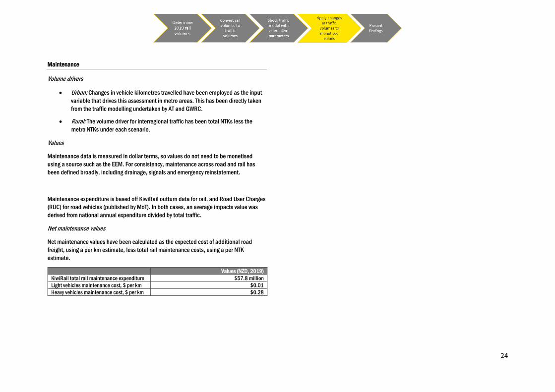
Maintenance
Volume drivers
• Urban: Changes in vehicle kilometres travelled have been employed as the input
variable that drives this assessment in metro areas. This has been directly taken
from the traffic modelling undertaken by AT and GWRC.
• Rural: The volume driver for interregional traffic has been total NTKs less the
metro NTKs under each scenario.
Values
Maintenance data is measured in dollar terms, so values do not need to be monetised
using a source such as the EEM. For consistency, maintenance across road and rail has
been defined broadly, including drainage, signals and emergency reinstatement.
Maintenance expenditure is based off KiwiRail outturn data for rail, and Road User Charges
(RUC) for road vehicles (published by MoT). In both cases, an average impacts value was
derived from national annual expenditure divided by total traffic.
Net maintenance values
Net maintenance values have been calculated as the expected cost of additional road
freight, using a per km estimate, less total rail maintenance costs, using a per NTK
estimate.
Values (NZD, 2019)
KiwiRail total rail maintenance expenditure $57.8 million
Light vehicles maintenance cost, $ per km $0.01
Heavy vehicles maintenance cost, $ per km $0.28
25
Stage 5: Limitations and assumptions of findings
A wide range of assumptions have been applied within this modelling exercise, leading to a
number of caveats and limitations:
• The scenarios were determined by MoT, and do not represent a forecast of likely
rail freight growth.
• This is a comparative, static model that demonstrates values at a single point in
time. All dollar values are reported in 2019 terms (e.g. adjusting 2018 EEM
figures for inflation).
• As noted on page 4, benefits are defined broadly for the purposes of this study,
extending to indirect costs and benefits affecting third parties.
• References to the EEM reflect that the majority of modelling was performed in
2019, prior to the publication of the Waka Kotahi Monetised Benefits and Cost
Manual.
• The study does not account for any behavioural change as a result of the differing
scenarios beyond the outputs of traffic modelling. For example changes to road
travel patterns or firm responses to alternative supply chain configurations.
• The calculation of benefits has been undertaken at the network level, in contrast
to the previous line by line analysis. This was due to data availability and the
challenge of accurately assigning rail freight to analogous road routes.
• Modelling assumes that all new trucks on the road consistently carry 9.6 tonnes
and does not attempt to adjust for empty return trips, beyond what is already in
the national average. Double handling of freight has not been considered.
• Traffic modelling results reflect a number of assumptions, detailed in Annex 2
and 3 below. Simple, proportional uplifts have been applied to reflect metro
patronage growth and truck conversation factors. This does not account for
dynamic interactions, cumulative impacts or network capacity limits.
• Congestion costs only include time delays and exclude any benefits of increased
travel time reliability.
• Safety impacts are based on national averages, i.e. the ratio of incidents divided
by total NTKs/Kms. Neither subnational safety profiles nor the cause of crashes
is considered in the analysis.
• The assessment does not estimate the relationship between congestion and
driver frustration. Greater congestion may, in reality, lead to a higher rate of
crashes.
• Rail deaths and injuries may include suicides and level-crossing incidents. Such
incidents are unlikely to scale with rail freight volumes, so may inflate the safety
costs of rail relative to road.
• National Road User Charges (RUC) revenue is used as a proxy for total road
maintenance costs. The difference between rail and road maintenance costs, and
be extension the value of rail, would be higher if the full cost of replacements
were included.
• Emissions factors for GHGs are based on published MfE guidance. Published
factors for heavy vehicles are specific to small trucks (<7,500kg), so are adjusted
to reflect the full HGV vehicle fleet (almost 80% of which are larger).
• Other emissions (NOx, SOx and PMx) calculations are based on a combination of
NZTA, MfE and MBIE data. As the Vehicle Emissions Prediction Model (VEPM)
does not contain comparable road and rail data, national MBIE data is instead
applied to ensure a consistent source. A more detailed discussion of this
methodology is provided on page 23.
• Air pollution impacts are calculated on a per-tonne basis and do not account for
sources, receptors, terrain or meteorology. NOx and SOx are calculated on a net
basis (i.e. road emissions minus rail emissions). PM is assumed to be exclusive
to road, reflecting that research focusses on the effects of such emissions in
enclosed environments or coal engines.
• PM2.5 impacts are uplifted to reflect published PM2.5 -> PM10 conversion
rates.
26
A
Appendices
27
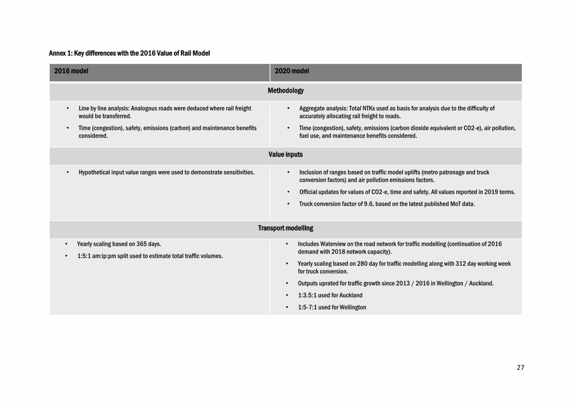
Annex 1: Key differences with the 2016 Value of Rail Model
2016 model 2020 model
Methodology
• Line by line analysis: Analogous roads were deduced where rail freight
would be transferred.
• Time (congestion), safety, emissions (carbon) and maintenance benefits
considered.
• Aggregate analysis: Total NTKs used as basis for analysis due to the difficulty of
accurately allocating rail freight to roads.
• Time (congestion), safety, emissions (carbon dioxide equivalent or CO2-e), air pollution,
fuel use, and maintenance benefits considered.
Value inputs
• Hypothetical input value ranges were used to demonstrate sensitivities. • Inclusion of ranges based on traffic model uplifts (metro patronage and truck
conversion factors) and air pollution emissions factors.
• Official updates for values of CO2-e, time and safety. All values reported in 2019 terms.
• Truck conversion factor of 9.6, based on the latest published MoT data.
Transport modelling
• Yearly scaling based on 365 days.
• 1:5:1 am:ip:pm split used to estimate total traffic volumes.
• Includes Waterview on the road network for traffic modelling (continuation of 2016
demand with 2018 network capacity).
• Yearly scaling based on 280 day for traffic modelling along with 312 day working week
for truck conversion.
• Outputs uprated for traffic growth since 2013 / 2016 in Wellington / Auckland.
• 1:3.5:1 used for Auckland
• 1:5-7:1 used for Wellington
28
Annex 2: GWRC traffic modelling
The following represents an abridged version of the technical note provided by the GWRC.
Multiple scenarios were run due to the four stage model design of the WTSM and to enable
a greater understanding of flows and results.
The WTSM is a strategic (macro) model that was developed to inform high level transport
policy and planning.
• The current base year for WTSM is 2013.
• Congestion is potentially underrepresented as WTSM models an average 2hr
period (thus averaging congestion during the peak 2hr as opposed to
representing congestion during the peak of the peak) and has a relatively coarse
representation of intersections and traffic blocking back (both areas where
delays occur)
• HCV are represented as part of the vehicle flows and the disruption due to HCV
(as compared to cars) is likely underrepresented.
It should be noted that WTSM represents vehicle demand flows rather than actual flows.
Therefore it assumes that all demand can get through the network to reach its final
destination. In reality, and of relevance to the interpretation of the removal of rail results,
the demand flows estimated by WTSM would result in significant delays and be unlikely to
be accommodated by the network within the modelled 2hr period.
• Changes to the freight volumes to & from the port alone result in very little
changes to other vehicles and the PT network.
• A 20% increase in Rail passengers results in a decrease in Bus patronage as well
as in vehicle trips. The main drop is in bus numbers; the drop in car numbers is
smaller, particularly percentage wise, although in the short-term the drop in
vehicle numbers could be greater as the modelling includes the impact of trip re-
distribution
• The removal of the rail network results in a major mode shift to cars and buses in
the short term.
• Over the longer term, the removal of the rail network could result in major trip re-
distribution (people change destination away from Wellington CBD in response to
change in accessibility) and mode shift to buses (assuming the capacity is
provided), lessening the modal shift and potential increase to cars on SH1 / SH2
into Wellington
Modelling the no rail network, 120% volume scenario
Combination of a decrease in HCV to/from port, with IVT parameters identified in previous
runs to reflect a scenario where there is both a reduction in truck volumes and an increase
in rail patronage. A full model run is undertaken for this scenario.
Modelling the no rail network, current volumes scenario
Increase in HCV to/from port + run assignment only model without rail network and with
adjusted car and PT demand matrices, representing the possible shorter term impact of a
‘no rail network’ scenario that does not include trip re-distribution and mainly focusses on
re-assignment.
The results should be considered as indicative, particularly as the tests where the rail
network is removed go beyond the bounds of what WTSM is normally used and designed
for.
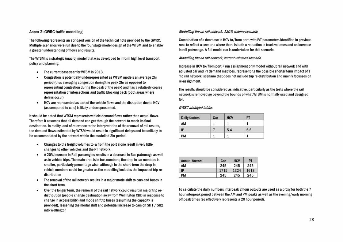
GWRC abridged tables
Daily factors Car HCV PT
AM 1 1 1
IP 7 5.4 6.6
PM 1 1 1
Annual factors Car HCV PT
AM 245 245 245
IP 1715 1324 1613
PM 245 245 245
To calculate the daily numbers interpeak 2 hour outputs are used as a proxy for both the 7
hour interpeak period between the AM and PM peaks as well as the evening/early morning
off peak times (so effectively represents a 20 hour period).
29
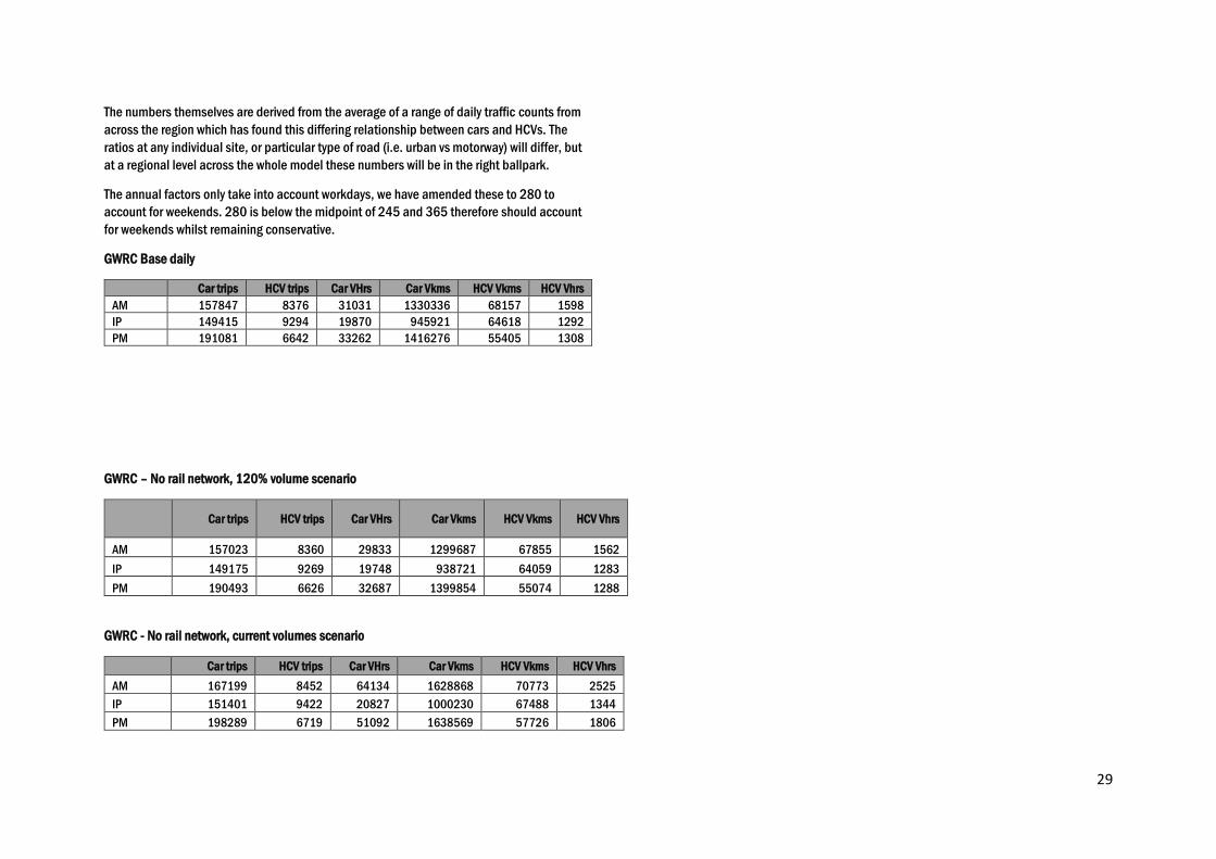
The numbers themselves are derived from the average of a range of daily traffic counts from
across the region which has found this differing relationship between cars and HCVs. The
ratios at any individual site, or particular type of road (i.e. urban vs motorway) will differ, but
at a regional level across the whole model these numbers will be in the right ballpark.
The annual factors only take into account workdays, we have amended these to 280 to
account for weekends. 280 is below the midpoint of 245 and 365 therefore should account
for weekends whilst remaining conservative.
GWRC Base daily
Car trips HCV trips Car VHrs Car Vkms HCV Vkms HCV Vhrs
AM 157847 8376 31031 1330336 68157 1598
IP 149415 9294 19870 945921 64618 1292
PM 191081 6642 33262 1416276 55405 1308
GWRC – No rail network, 120% volume scenario
Car trips HCV trips Car VHrs Car Vkms HCV Vkms HCV Vhrs
AM 157023 8360 29833 1299687 67855 1562
IP 149175 9269 19748 938721 64059 1283
PM 190493 6626 32687 1399854 55074 1288
GWRC - No rail network, current volumes scenario
Car trips HCV trips Car VHrs Car Vkms HCV Vkms HCV Vhrs
AM 167199 8452 64134 1628868 70773 2525
IP 151401 9422 20827 1000230 67488 1344
PM 198289 6719 51092 1638569 57726 1806
30
Annex 3: AT traffic modelling
The following represents an abridged version of the salient points of discussion with AT.
The transport model used is a Macro Strategic Model (MSM) which is a four stage model.
The model is based on land use and trip generation and matches trip ends and
assignments based on time costs and estimates.
The base year of the model is 2016, updates to congestion have not been incorporated due
to delays in the latest census data.
The base model was amended to include the Waterview tunnel on the transport network in
the transport model runs. Network capacity is based on 2018 parameters.
20% increase in rail scenario
The modelling scenario of a 20% increase in rail patronage proved difficult. Multiple runs
were undertaken to establish the 20% increase. Exogenous changes were made to obtain
the number namely changing:
• Frequency of rail multiplied by 1.4 taking headway (1/1.4)
• SS runtime *.07 (Speed/0.7)
• Rail fare * 0.7
• $ per km *0.7
• Boarding $ *0.7
The station dwell was kept constant for the purposes of the analysis.
Yearly conversion factor
Most transport modelling requests are for the effects on the AM peak interpeak and PM
peak where it is known traffic congestion is at its worse in Auckland. There is currently no
assignment for outside these times.
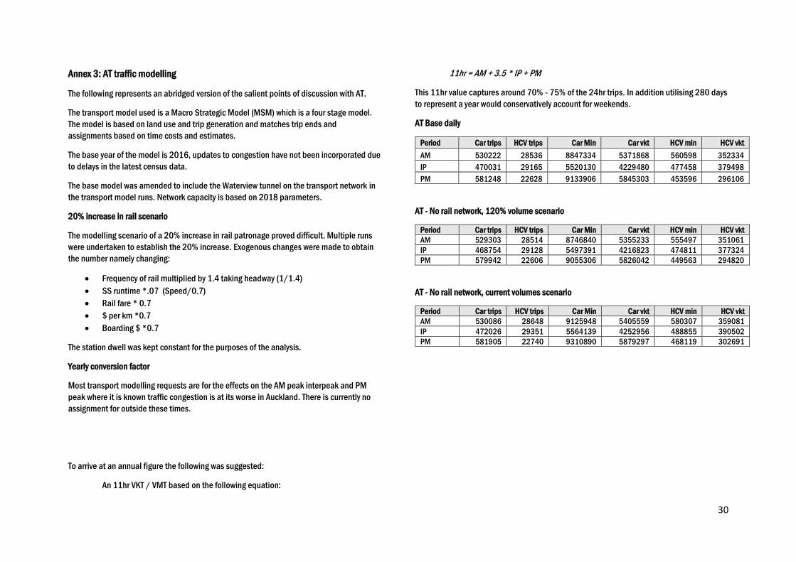
To arrive at an annual figure the following was suggested:
An 11hr VKT / VMT based on the following equation:
11hr = AM + 3.5 * IP + PM
This 11hr value captures around 70% - 75% of the 24hr trips. In addition utilising 280 days
to represent a year would conservatively account for weekends.
AT Base daily
Period Car trips HCV trips Car Min Car vkt HCV min HCV vkt
AM 530222 28536 8847334 5371868 560598 352334
IP 470031 29165 5520130 4229480 477458 379498
PM 581248 22628 9133906 5845303 453596 296106
AT - No rail network, 120% volume scenario
Period Car trips HCV trips Car Min Car vkt HCV min HCV vkt
AM 529303 28514 8746840 5355233 555497 351061
IP 468754 29128 5497391 4216823 474811 377324
PM 579942 22606 9055306 5826042 449563 294820
AT - No rail network, current volumes scenario
Period Car trips HCV trips Car Min Car vkt HCV min HCV vkt
AM 530086 28648 9125948 5405559 580307 359081
IP 472026 29351 5564139 4252956 488855 390502
PM 581905 22740 9310890 5879297 468119 302691