Embed Size (px)
Citation preview
The Value of Land Use Patterns and Preservation Policies∗
Martin D. Heintzelman
Economics and Financial Studies
School of Business
Clarkson University
E-mail: [email protected]
Phone: (315) 268-6427
June 23, 2009
PRELIMINARY DRAFT - Do not cite of quote without permission of the author.
∗Martin D. Heintzelman is Assistant Professor, School of Business, Clarkson University. I would like tothank seminar participants at Clarkson University and the NAREA 2009 Annual Meeting for useful thoughtsand feedback. I would also like to acknowledge the research assistance of Patrick Becker, Peter Claus-Landi,and Dustin Greszkowiak. All errors are my own.
DRAFT
1 Introduction
Beyond the basic characteristics of a home such as its size and the size of the property upon
which it sits, within a given real estate market, much of a home’s value derives from the
amenities provided by its location. These locational factors include convenience (distance
to places of employment, shopping, highways, rail stations), amenities (local land-uses,
open-space, parks), disamenities (distance to waste facilities, rail-lines, industrial zones),
as well as regulatory impacts (zoning, historic districts). Policy-makers have long tried to
impact property values through zoning and city/town/urban planning, as well as explicit
policies to preserve/protect open-space, farmland, and wildlife habitat. This paper uses a
fixed-effects, differences-in-differences, approach to examine the impacts of local land uses,
zoning rules, and other locational factors on property values, as well as those of policies
designed to preserve open-space and historic sites, and simultaneously provide for affordable
housing. It focuses on the state of Massachusetts and that state’s Community Preservation
Act (CPA).
Briefly, the CPA is a policy enacted at the town level which allows towns to leverage a
property tax surcharge with state matching funds for the purposes of Open Space Preser-
vation, Historic Preservation, and Community (affordable) Housing. The policy, in place
since 2001, has been enacted slowly over time by towns, so that, to date, 142 towns out of
a possible 351 have enacted the CPA, and these enactments have been spread over 9 years
(2001-2009). In fact, there are towns just now taking up the measure. One of the aims of
this paper is to study the ex post impacts of CPA passage on property values.
Of course, while this paper is focusing on one state and one particular policy, this is
hardly an issue that is isolated to Massachusetts. Since 1988, there have been some 1,686
conservation measures approved by voters (out of 2,233 total measures on ballots) in at least
2
DRAFT
43 states. Altogether, these measures have set aside some $53 Billion for conservation.1
Massachusetts is also not the only state to have a matching funds program. New Jersey’s
Green Acres Program is just one other example of a similar policy which provides state aide
to local communities seeking to preserve open space.
There is an extensive literature on the economic values of varying land-uses, mostly
focusing on the value of open-space, variously defined.2 This literature consistently finds
that open-space in its many guises (cropland, pasture, forest, urban parks, etc.) is positively
related to property values. What is less consistent is the magnitude of this effect. There
is considerable heterogeneity both between studies and even in different areas within the
same study (Heintzelman, 2009). Most often, this literature has used cross-sectional data to
explore the value of open space, and is thus susceptible to omitted variables bias. A critical
contribution of this piece is to use a ‘panel’ like dataset enabling me use a fixed-effects
analysis which greatly reduces the range of possible omitted variables.
The literature on voter referenda for open-space preservation is considerably less deep.
Kotchen and Powers (2006) and Nelson et. al. (2007) analyze what drives the appearance
and success of these referenda in states and local communities. They find that preservation
is a normal good - wealthier communities are more likely to vote for preservation. Kotchen
and Powers (2006) also find that preservation is most likely in suburban (not urban, not
rural) communities where development pressure is perceived to be highest. Only Heintzel-
man (2009) has previously studied the impacts of these referenda, and a small sample size
prevents him from drawing firm conclusions about the impacts.
My results indicate that, on average, passage of the CPA reduces property values by
about 1.5% in Massachusetts towns. However, when I allow the CPA effect to differ by
county, I find some heterogeneity - it increases property values in some communities and1Data from the LandVote database maintained by the Trust for Public Land, http://www.tpl.org/2See McConnell and Walls (2005) for a survey or Waltert and Schlapfer (2007) for a meta-analysis of this
literature. For more recent contributions see Heintzelman (2009) and Kuminoff (2008), amongst others.
3
DRAFT
reduces them in others. There is limited evidence on the extent to which different local
spending priorities impact the overall effect. I also find that cropland and pasture, as well
as low-density residential development, are the most preferred local land-uses, and that
homes are more expensive as one increases distance to highways and active rail lines.
Section 2 provides a detailed background information on the Community Preservation
Act. Section 3 describes the research methodology. Section 4 provides the results, Section
5 interprets and extends the basic results, and Section 6 concludes.
2 Policy Background
The Massachusetts Community Preservation Act was passed in 2000. It is a state program
which provides matching funds to those towns who choose, through a referendum, to enact
property tax surcharges of up to 3% and spend the additional funds (both those raised
through the surcharge and the matching funds) on open-space preservation, historic preser-
vation, and ‘community’ (affordable) housing. In practice, money has also been spent to
provide recreational facilities.3 Towns are required to spend at least 10% of funds raised
on each of the three core areas, and are free to allocate the remaining 70% as they wish.
In general, towns appoint a Community Preservation Committee to recommend projects
to be funded, and final decisions must be approved by the town meeting. The funds are
held in separate from general town accounts and are not available to address other local
spending priorities. The tax surcharge may include any or all of three tax exemptions: for
low income households, for the first $100,000 of property value, and for commercial and
industrial properties. Finally, the adoption process is a two-stage process: first, the lan-
guage of the referendum and parameters of the policy (surcharge, exemptions) are approved3From 2001-2007, the state matched locally raised funds at a rate of 100%. In 2008, this fell to 67% and
may be as low as 35% in 2009. The state matching funds come from a fee charged for deed transactions inthe state.
4
DRAFT
either through the town meeting or through a petition drive; second, the referendum must
be approved in a referendum vote.
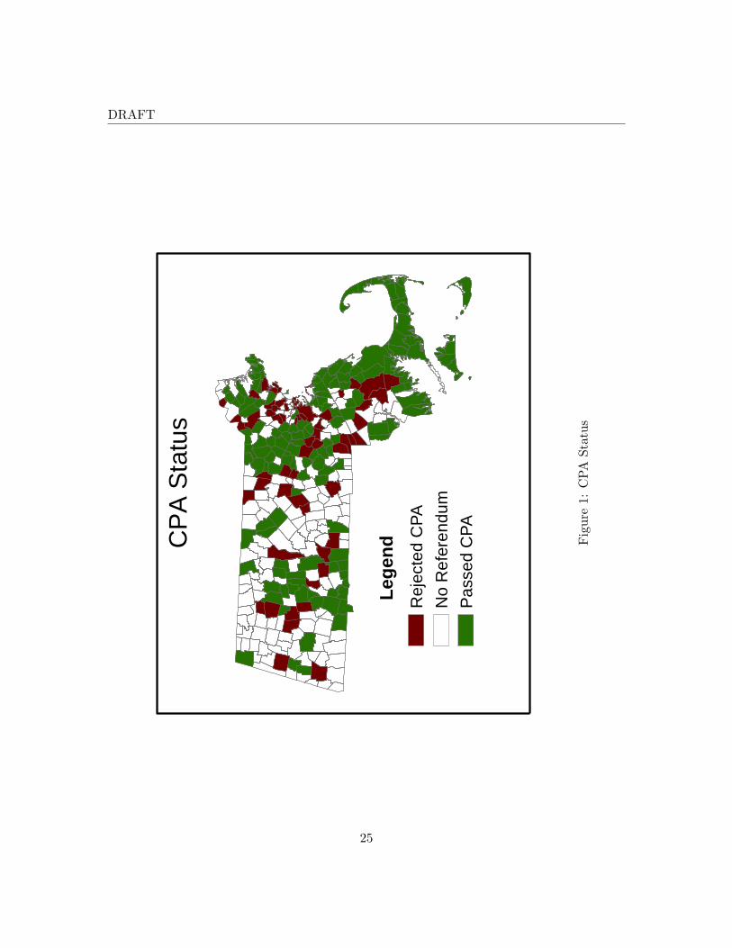
As of June 2009, 142 communities have adopted the CPA out of the 351 towns and
cities in Massachusetts. In addition to these communities, some 58 communities have re-
jected the CPA at the referendum stage.4 Figure 1 shows a map of the towns and cities
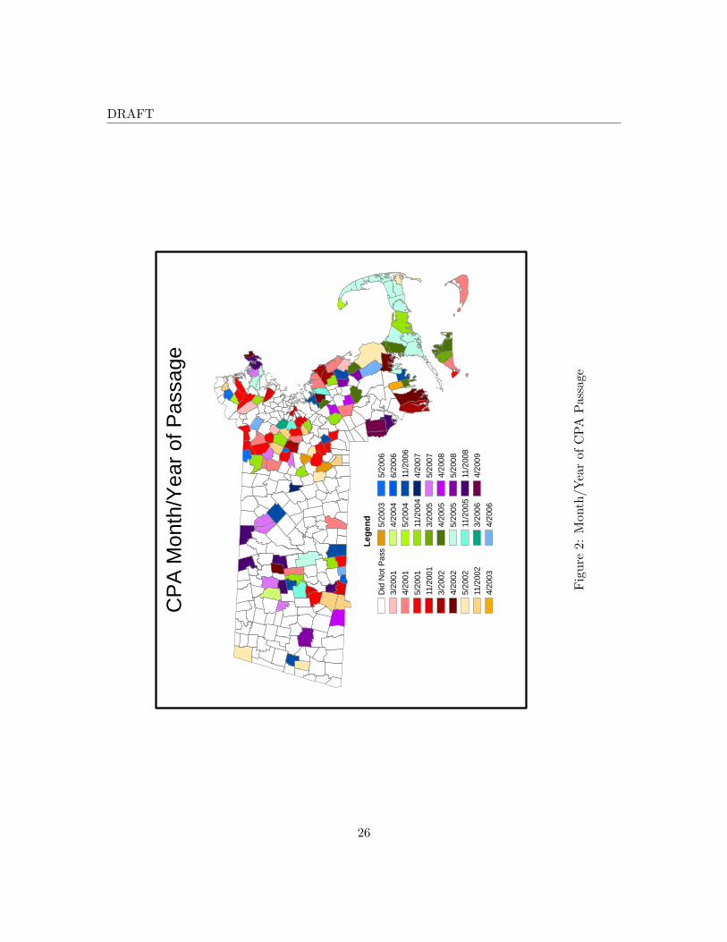
of Massachusetts by whether they have passed or rejected the CPA. Figure 2 shows a map
of enacting communities color -coded by the date of adoption. According the Commu-
nity Preservation Coalition, an organization that advocates for communities to adopt the
CPA, “Using CPA funds, municipalities have preserved 10,274 acres of open space, includ-
ing important wetland resources such as lakes, rivers, and saltwater ponds. In the area
of affordable housing, CPA funds have allowed for the creation or rehabilitation of more
than 2,300 affordable housing units and the development of hundreds of innovative afford-
able housing programs. Finally, more than 1,300 appropriations for historic preservation
projects and over 500 recreation projects have been approved under the program.”5 Of
those communities that have passed the CPA, 52% choose the highest potential surcharge
rate of 3%. The average surcharge rate is 2.227%. 75.35% of enacting towns exempted low
income households and nearly 79% exempted the first $100,000 in home value. Only 3.5% of
towns exempted commercial and industrial property. No communities that have ever passed
the CPA have subsequently withdrawn from the program, and three towns have, subsequent
to initial passage, passed a second referendum to increase the surcharge rate. According
to preliminary data from the Massachusetts Department of Revenue (DOR), there is quite
a bit of variation in how the CPA money that has been raised so far has been spent. On
average, towns have spent about 35% of CPA funds on Open Space, 22% on Affordable
Housing, 13.2% on recreation, and 29.8% on Historic Preservation.419 Communities initially rejected the CPA and then later enacted it.5“Summary of an Act to Sustain Community Preservation, SB 90”, available at
http://www.communitypreservation.org/CPALegislation.cfm.
5
DRAFT
Intuitively, it is not clear what impact we should expect of the CPA on property values
as there are a number of possible effects acting simultaneously. A first thought is that towns
are opting into the program, so presumably a majority of voters in the enacting towns think
that, on average, the policy will be good for their town, and in turn, would be good for
property values. For one thing, through the matching funds, towns are essentially able to
purchase public goods at a reduced price - provided that all of the outcomes of the CPA are,
in fact, public goods. Basic consumer theory tells us that consumers (in this case, towns)
can not be made worse off by a decrease in prices. However, there is reason to believe
that many voters may have other reasons to vote for the CPA, regardless of the impact on
property values. For instance, renters, or those meeting surcharge exemptions, if in place,
stand only to gain from the CPA as they receive additional public goods at no additional
cost. This implies that a passing vote does not necessarily imply expectations of average
improvements in social welfare.
Ignoring the political economy aspects of the problem, it is still not clear what the
impact of the CPA should be. It simultaneously includes both an increase in taxes and an
increase in goods provision. Following Brueckner (1982), average property values will be
highest when the level of public goods provision is optimal (over-provision implies taxes too
high, under-provision implies services (and taxes) too low). So, if the CPA is moving towns
towards the optimum it will increase property values, but if it is pushing them beyond the
optimum it will lower property values. In addition, while the tax-cost of the CPA is clear up
front - consumers presumably have a very good idea of what the surcharge will imply about
their annual tax burden, the benefits of the program, particularly at the time of the vote,
are unclear. Much of the money being raised is simply being set aside for future purchases,
and there is not ex-ante obligation for the town to publicize the expected uses of the money.
This implies that consumers, in purchasing homes, may be very aware of the taxes they are
paying, but less aware about the benefits being provided. There are also supply effects of
6
DRAFT
the CPA - restrictions on development restrict to supply of housing, which should increase
property values. However, the provisions for affordable housing may undercut these effect by
providing for additional high-density residential development (which both increases supply
of housing and provides a public ‘bad’ in the sense that high density residential housing
generally reducing property values).
3 Data and Empirical Strategy
I employ a standard hedonic regression analysis to estimate the effects of land-use charac-
teristics and CPA passage on residential transaction prices. I have data on all residential
property sales in the state of Massachusetts for the years 2000-2007. This data includes the
sales price, date, and location of the home as well as a number of structural characteristics
including lot size, interior size, bedrooms, bathrooms, and some indication of the ‘style’
of the home. I use GIS to attach geographical information (land-use, zoning information,
distance to highways, rail lines, rail stations). In addition, I include monthly, town-level,
unemployment rate data from the Massachusetts Department of Revenue (DOR). Finally,
I include town-level data on the CPA including the date of passage, the surcharge rate, and
included exemptions, as well as preliminary information on CPA expenditures, also from
the DOR. After accounting for erroneous observations and those missing critical pieces of
information (most often the date of a home’s construction), I am left with 623,163 obser-
vations.6
This paper, in a sense, is doing double duty by estimating traditional hedonic effects
in addition to the treatment effect of the policy, and to successfully estimate both, I must
overcome some econometric obstacles. A major issue in estimating hedonic models, gen-
erally, is the problem of omitted variables (Parmeter and Pope, 2009). There are almost6The base dataset, from The Warren Group, contained 798,202 observations, and so I have been able to
retain 78% of the original observations.
7
DRAFT
innumerable factors which go into the value of a home, and many of these characteristics
are unobservable to the researcher. If these unobservables are correlated with any of the
observed characteristics, ones estimates will be biased. Similarly, in estimating treatment
effects, there may be selection bias if the outcome variable (in this case, property values)
is correlated with a factor which, in turn, is correlated with an observation receiving the
treatment (Greenstone and Gayer, 2009). A recent literature in environmental economics
has sprung up to adapt quasi-experimental approaches from other fields of economics to
environmental issues in order to deal with these issues.7
There are three broad classes of quasi-experimental approaches: Differences-in-Differences
(Fixed-effects), Instrumental Variables, and Regression Discontinuity (Greenstone and Gayer
(2009), Parmeter and Pope (2009)). In this paper I apply the first of these, the Differences-
in-Differences approach. This approach takes advantage of the ‘panel’ nature of my dataset
to help solve both of the problems (omitted variables, selection bias) identified above. By
including census block, census block-group, or even property-level fixed effects, I am able
to control for any constant but unobserved factors that act at the local level and may be
correlated both with property values and the explanatory variables of interest. Suppose
for instance that towns with higher average incomes are more likely to pass the CPA. In
the absence of fixed effects, I would observe a spurious positive correlation between passage
of the CPA and property values. However, by including the fixed effects, and since town
relative average incomes are likely to be relatively constant over a reasonable sample period,
I am now controlling for this factor (and any other constant characteristics). Essentially,
my regression coefficients will be the average within-group (census block, block-group, or
property) impact of each explanatory variable.
One downside to this approach is that successful estimation will require sufficient within-7See, for example, Parmeter and Pope (2009), Greenstone and Gayer (2009), and Klaiber and Smith
(2009). For an excellent survey of general program evaluation methods, see Imbens and Wooldridge (2009).
8
DRAFT
group variation in each explanatory variable. Obviously, the smaller the groups the more
factors that are being controlled for in the fixed-effect, but also the less variation that will
be observed and the less statistical power I will have. As a result, I test the robustness of
my results to changing the scale of the fixed-effect, and will look to balance these competing
interests in determining the optimal scale.
What remains as potential confounding factors in this analysis - in particular the estima-
tion of the treatment effect - are factors which are not constant over time. If there are any
of these factors which are changing co-incident with both property values and the passage
of the CPA in a community, than I could be mis-attributing changes in property values to
the CPA. This would be of particular concern if I had only a small sample of communities
being treated. With my large sample, while there may be these types of factors affecting
individual communities, for me to mistake an effects for that of the CPA it would have
to be happening in most of the 140 treatment communities at the same time as the CPA
(which varys considerably amongst the treatment communities), which seems unlikely. To
help with this matter, however, I do include a number of time-dependent controls. To net
out any macro-level (trends for the full sample) trends, I include year dummy variables. I
also include month dummies to account for seasonal effects. Finally, I normalize sales prices
according the the Federal Housing Finance Agency’s (FHFA) House Price Index. This is
calculated at the U.S. Census MSA level (in Massachusetts, effectively, counties or groups
of counties). Together, these three adjustments should fully de-trend and de-seasonalize the
data, and allow me to isolate town-level effects, like the CPA.
In conducting a hedonic property-value analysis one must also be alert to spatial de-
pendence and spatial auto-correlation.8 A dataset exhibits spatial dependence if, in this
context, property values for nearby properties are not determined independently of one
another. That is, if one property’s value depends on the value of its neighbor’s. Spatial8See LeSage and Pace (2009) for a complete treatment of this subject.
9
DRAFT
auto-correlation, similarly, is when the error terms for neighboring (or nearby) properties
are not independent of one another. Both of these concerns can be expected in hedonic
property-value models. A fully general spatial econometric estimation approach would as-
sume a spatial weighting matrix which would, for any pair of properties describe how ‘close’
they are to each other, and, assuming that this matrix is correctly specified, one can con-
trol for both spatial dependence and spatial autocorrelation. Given the size of my dataset,
however, so general an approach is extremely computationally intensive. Conveniently, how-
ever, there are some simpler ways to control for spatial issues. First, spatial dependence
can be partially controlled for by the local-area fixed effects. In effect, this approach allows
for spatial dependence within groups (as defined at the census block or block-group level),
but not across groups. Secondly, spatial autocorrelation can be controlled for in a similar
manner by allowing for error clustering within defined groups (not necessarily at the same
spatial level at the fixed-effects groups), which simultaneously makes the calculated error
terms robust to heteroskedasticity.9
Following Bertrand, Duflo, and Mullainathan (2004) and Parmeter and Pope (2009),
the form of the estimated equation can then be written:
pijt = λt + αj + zjtβ + xijtδjt + ηjt + εijt (1)
where pijt represents the price of property i in group j at time t; λt represents the set of
time dummy variables; αj represents the group fixed effects; zjt represents the treatment
variable (the CPA); xijt represents the set of other explanatory variables; and ηjt and εijt
represent group and individual-level error terms respectively.
Another issue in any analysis of land-use issues values is the proper measurement of land-
use. Perhaps the most frequent measure is the distance to the nearest parcel of a certain9Essentially, combined, these fixes allow for spatial weighting matrices containing ‘1’s for all observations
within groups and zeros elsewhere.
10
DRAFT
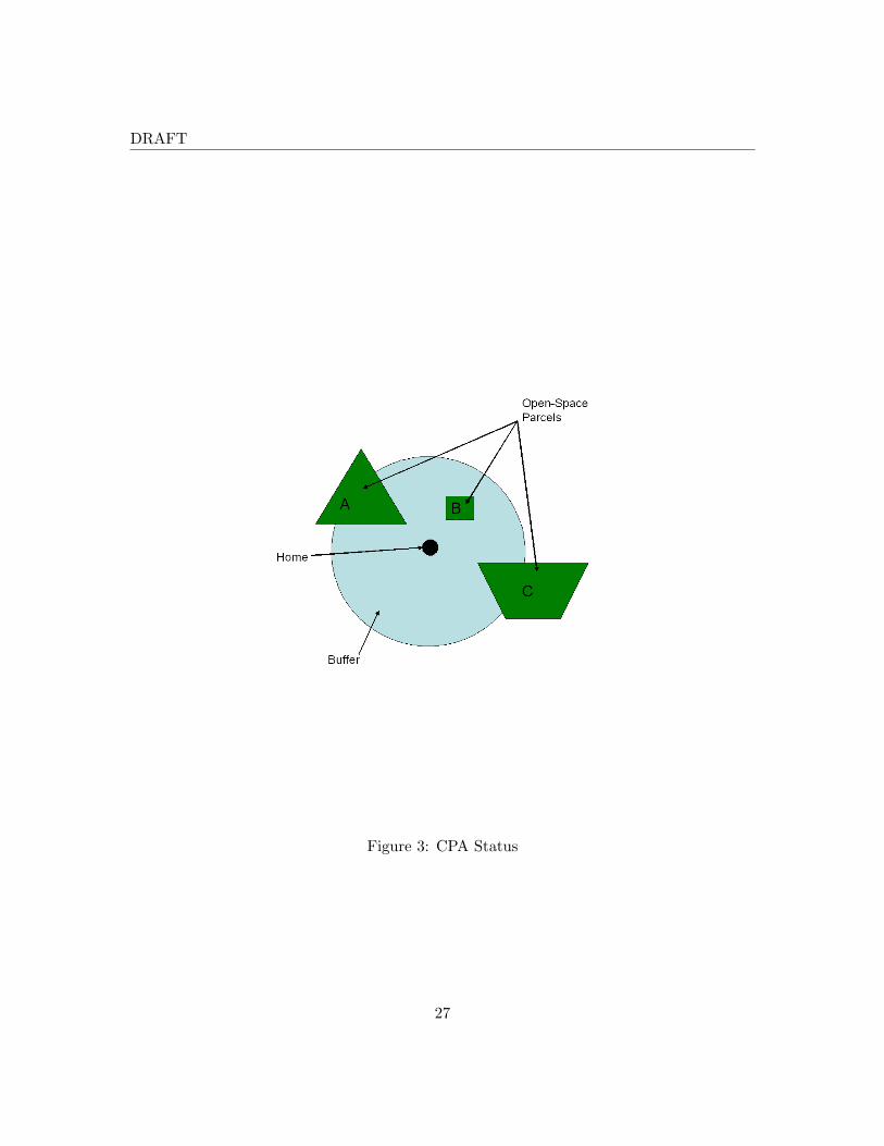
type. While this measure has clear merits I do not believe it is the whole story. Instead,
I measure the total acreage of parcels of each type which intersect a buffer around the
transacted properties.10 This, I believe gives a more complete picture of possible impacts.
Figure 3 provides an example of this measure. I do employ a distance measure for other
factors such as the distance to highways, highway exits, active rail lines, and passenger rail
stations.
4 Results
I begin by regressing the log of the normalized sales price (as discussed above) on the
full range of possible explanatory variables, including home characteristics, local land-use
characteristics, the zone in which the home is located, a series of other locational variables,
the monthly unemployment rate, and, finally, the CPA status in the town in which the home
is located on the date of the sale.11 Table 1 provides summary statistics for the variables
included in this analysis. I include two primary measures of CPA status - a simple dummy
variable for whether or not the CPA had passed in that community prior to the sale date
and secondly, the effective surcharge rate passed in the community (zero for those towns
that had not yet enacted the CPA). As mentioned above, I also vary the geographic scale
of the fixed effects to test the robustness of the estimates to this important assumption.
Table 2 provides the results of these regressions.
Regressions 1 and 2 include the CPA dummy, while Regression 3 uses the surcharge rate.
Regression 1 uses census block fixed effects, while Regressions 2 and 3 use census block-
group fixed effects. I will focus mostly on Regressions 2 and 3 in the discussion below. This10I do not have information on parcel boundaries, so instead use point estimates of each home’s location
based on 9-digit zipcodes.11The semi-log specification is chosen to better allow comparisons to other literature in this area, specif-
ically, Cropper, Deck, and McConnell (1988). However, recent evidence by Kuminoff, Parmeter, and Pope(2009), suggests that more flexible functional forms may be superior. This is a next step in this analysis.
11
DRAFT
is because the results at this broader geographic scale of fixed effects are generally more
significant. This is intuitive, and consistent with Kuminoff, Parmeter, and Pope (2009).
As we increase the scale of the fixed-effect, we perhaps open ourselves up to more omitted
variables, but simultaneously allow for more variation in the included covariates which gives
our estimates more power. At the block-group level, however, we still have 4,991 groups,
each averaging only 125 observations.
The CPA dummy coefficient gives the percentage change in price for a binary change
to the value of the dummy variable. This indicates that passage of the CPA results in a
1.43% to 1.77% reduction in home prices. Similarly the surcharge rate coefficient gives the
percentage change in price for a unit increase in the surcharge rate, and implies a 0.65%
reduction. These results are broadly consistent with each other since most towns choose a
3% surcharge.
Strangely, the monthly unemployment rate is positively related to home prices. This
result is robust to changing the specification of the property value/unemployment rate
relationship. This must reflect some omitted variable that is causing a spurious correlation.
Thankfully, however, omitting the unemployment rate from the analysis does not change
the estimate of the CPA coeffcient, which indicates that whatever is driving this result, it
is not affecting our estimate of the CPA effect.
The distance variables suggest, as we would expect, that people will pay a premium
for increased distance from highways and active rail lines. The estimates for exits and
stations, included in an attempt to separate convenience aspects of transportation from
the associated dis-amenities are not significant, although when using the block-group fixed
effects, the station variable is of the right sign. All of the home characteristic variables
are positive and significant with the exception of age which is negative, but decreasing at
a decreasing rate. Condominiums are cheaper than single-family homes and relative to
an excluded ‘other-style’ category, Colonials and Contemporaries are more expensive while
12
DRAFT
ranches and flats are less expensive.
The type of ‘zone’ a home is in also affects its value. Relative to an excluded ‘other’
category, commercial, industrial, high-density residential, and conservation zoning, not sur-
prisingly, generally have negative impacts on home prices, while most other residential
categories are positive or insignificant. The conservation zoning result is perhaps most in-
teresting. It suggests that the limitations inherent with such zoning policies are harming
property values, and this may help explain the negative impact of the CPA - if passage of
the CPA implies that a significant sample of homes will be subject to increased restrictions
on development, this may reduce average prices.
Finally, many of the land-use coefficients are significant. Cropland, pasture, and low-
density residential land-uses are positively related to home prices. High and medium density
residential development, as well as commercial, urban open space, transportation, and waste
land-uses are negatively related to home prices. Industrial development is also negatively
related, but it is not quite significant at the 90% level. All of these results are to be
expected, except, perhaps for the urban open space result. There may be congestion effects
associated with use of these parks which are driving this result. The results presented also
highlight the effect of changing the geographic level of the fixed effect. When fixed effects
are calculated at the census block level, the lack of variation within blocks seems, indeed, to
lead to insignificant estimates of the land-use effects, but this is reversed when expanding
the fixed-effects to the census block-group level.12
Given the size of my dataset and the relatively large sample period, there are a significant
number of properties which sell more than once in my sample. Limiting analysis just to
these observations gives us a true fixed-effects model and completely eliminates any concerns
about omitted variables (other than, as discussed above, factors changing coincident with12There are 69,320 census blocks represented in my data, with an average of only 9 observations per block.
There are only 4,991 census block groups represented in the data, with an average of about 125 observationsper block-group.
13
DRAFT
the referendum). This gives the cleanest possible estimate of the referendum effect, and
results are presented in Table 3. The result from the full-sample analysis, that the CPA
negatively impacts property values is confirmed in this analysis, and the magnitude is
almost identical to that estimated above. This analysis also includes variables representing
the running sum of reported CPA expenditures in each of four areas (open-space, affordable
housing, recreation, and historic preservation). All seem to be positively related to property
values, but only historic preservation spending is significant. An alternative specification
which included the share of each category as a percentage of total reported spending gave
no statistically significant results.
5 Discussion
The regression coefficients described above indicate a negative and significant impact of
CPA passage on property values of about 1.5%, on average. It is straightforward to put
this number in perspective. For the average home, this reduction amounts to a reduction in
price of about $1,991. On the other hand, the average increase in taxation from the CPA
is about $112 per year. The present value cost of this additional tax, at a 5% interest rate
is $2,352 and so the tax is being capitalized into property values at a rate of about 85%.
This rate of tax capitalization is somewhere between the consensus estimates from the tax
capitalization literature by Palmon and Smith (1998) and Oates (1966) of between 56% and
66% and that predicted by Ricardian equivalence - 100%.
As with any regression coefficient, however, this estimate of the referendum effect is
simply an average effect across the sample. To see the extent of variation away from this
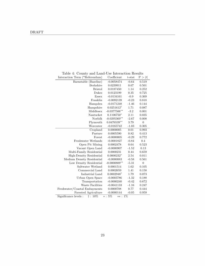
estimate, I interact the CPA dummy with county dummies and with the land-use measures.
Table 4 provides the estimates of the interaction terms from this regression. 13 There13The estimates for the other variables, the same as those in Table 2 are very similar to those in the base
regression.
14
DRAFT
are significant negative impacts of the CPA in two counties, Middlesex and Norfolk, and
significant positive effects in Hampshire, Nantucket, and Plymouth counties. The point
estimates range from a 3.7% decline in values in Middlesex County to a 4.7% increase in
values in Plymouth County. The large negative impacts in Middlesex and Norfolk counties
may be helping to drive the overall negative average effect of the CPA since Middlesex and
Norfolk are two of the three largest counties in terms of number of observations. There are
no immediate explanations available to explain this result, although a possible explanation
for the Middlesex result is a very large share (31%) of existing CPA spending has been on
affordable housing, the second-highest in the sample. The Land-Use interaction results are
also very interesting. We see that high-density residential and industrial land have positive
impacts on the CPA effect, while low-density residential land has a negative impact on
the CPA effect. This suggests that those homes in more densely developed areas stand to
benefit more from the CPA than those in less densely developed areas, which is consistent
with intuition since open-space is presumably more scarce in more densely developed areas.
More generally, this observed heterogeneity in impact is consistent with prior literature
(Heintzelman (2009), Geoghegan (2003), Anderson and West (2006)), which has found the
same sorts of heterogeneity in estimating the value of open space preservation.
Similar to the true fixed-effects analysis including only repeat-sales, I tried including data
on spending in the full-sample regressions. I attempt a number of specifications, and very
few of them yield any significant results. One result that is consistent across specifications,
however, is that total spending is negative and significant while its square is positive and
significant. When these terms are included, the magnitude of the estimate for the effect of
the CPA is reduced, although it is still significant and negative. This suggests that larger
programs have larger negative effects, which is consistent with the result from estimating
the effect of the rate rather than just the CPA dummy. If I leave out the total spending
variables and instead include only categorical spending variables (rather than categorical
15
DRAFT
shares), expenditures on Open Space, Affordable Housing and Recreation have negative
impacts, although only that for Affordable Housing is significant, while expenditures on
Historic Preservation are positive, but insignificant. This gives some evidence that, of the
four categories, affordable housing is the least preferred and most likely to decrease property
values.
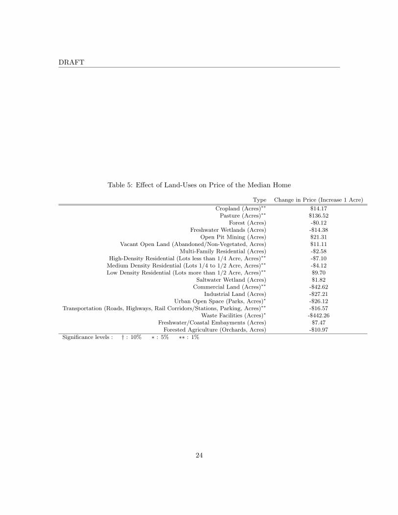
Moving to the measures of land-use, it is interesting to discuss these results with the aid
of a simple heuristic - what is the effect on sales price if 1 acre of land near a home changes
from an open space category (pasture, cropland, or woodland) to a developed category
(residential, commercial, industrial). Table 5 presents the results of asking this question for
the median home in the state-wide sample.14 Notice, as an example, that replacing an acre
of pasture with an acre of commercial development would reduce price by almost $180. Of
course, most commercial developments are at a considerably larger scale, implying much
larger price effects. The most preferred land-uses, which are also statistically significant,
are Pasture and Cropland, implying, perhaps, that there is something preferable about
farmland as opposed to other low-density uses - even conversion to low-density residential
development would lower neighboring home prices.
6 Conclusions
This paper provides evidence that preservation policies, while generally providing public
goods, and even when approved through a voter-referendum, may not be positively capi-
talized into home values. Using the quasi-experimental method of differences-in-differences
analysis, I find that, in the case of the Massachusetts Community Preservation Act, pas-
sage of the CPA has had an overall negative impact on property values of about 1.5%
in towns that pass the CPA. This effect is observed to be heterogeneous across counties14Only changes in prices from increases in acreage are presented. The results for decreases are, obviously,
almost identical and are thus omitted for simplicity.
16
DRAFT
and according to local land-use characteristics, with more densely developed areas seeing
more benefits than those less densely developed. Nonetheless, the land-uses that are at
least partially being targeted for preservation under the CPA do appear to have value for
homeowners, relative to more developed uses. While it remains somewhat of a puzzle why
towns would pass policies that are negatively affecting property values, it can explain why,
in many towns, passage of the CPA is controversial, and why more than half the towns in
Massachusetts still have not adopted the policy.15 There is some evidence that spending on
Community Housing helps to drive down the impact of the CPA, which is consistent with
intuition, but more work needs to be done to fully establish that point.15Of the 140 communities that passed the CPA before 2008, the median margin was 58% to 42%. In
addition, 58 towns rejected the measure, and another 151 towns have not put it to a vote.
17
DRAFT
References
Anderson, S. T. and West, S. E. (2006). Open space, residential property values, and spatial
context. Regional Science and Urban Economics, 36:773–789.
Bertrand, M., Duflo, E., and Mullainathan, S. (2004). How much should we trust differences-
in-differences estimates? Quarterly Journal of Economics, 119:249–275.
Brueckner, J. K. (1982). A test for allocative efficiency in the local public sector. Journal
of Public Economics, 19:311–331.
Cropper, M. L., Deck, L. B., and McConnell, K. E. (1988). On the choice of functional
form for hedonic price functions. Review of Economics and Statistics, 70(4):668–675.
Geoghegan, J., Lynch, L., and Bucholtz, S. (2003). Capitalization of open spaces into hous-
ing values and the residential property tax revenue impacts of agricultural easement
programs. Agricultural and Resource Economics Review, 32(1):33–45.
Greenstone, M. and Gayer, T. (2009). Quasi-experiments and experimental approaches to
environmental economics. Journal of Environmental Economics and Management,
57:21–44.
Heintzelman, M. D. (2010). Measuring the property-value effects of local land use and
preservation referenda. Land Economics. Forthcoming.
Imbens, G. W. and Wooldridge, J. M. (2009). Recent developments in the econometrics of
program evaluation. Journal of Economic Literature, 47(1):5–86.
Klaiber, H. A. and Smith, V. K. (2009). Evaluating rubin’s causal model for measuring
the capitalization of environmental amenities. NBER Working Paper 14957, National
Bureau of Economic Research.
Kotchen, M. J. and Powers, S. M. (2006). Explaining the appearance and success of voter
referenda for open-space conservation. Journal of Environmental Economics and Man-
agement, 52:373–390.
18
DRAFT
Kuminoff, N. V. (2008). Using a bundled amenity model to estimate the value of cropland
open space and determine an optimal buffer zone. Unpublished Working Paper.
Kuminoff, N. V., Parmeter, C. F., and Pope, J. C. (2009). Specification of hedonic price
functions: Guidance for cross-sectional and panel data applications. Working Paper
2009-02, Department of Agriculural and Applied Economics, Virginia Polytechnic
Institute and State University, Blacksburg, VA.
LeSage, J. P. and Pace, R. K. (2009). Introduction to Spatial Econometrics. Chapman and
Hall, CRC Press.
McConnell, V. and Walls, M. (2005). The value of open space: Evidence from studies of
non-market benefits. Report, Resources for the Future.
Nelson, E., Uwasu, M., and Polasky, S. (2007). Voting on open space: What explains the
appearance and support of municipal-level open space conservation referenda in the
united states. Ecological Economics.
Oates, W. E. (1969). The effects of property taxes and local public spending on property
values: An empirical study of tax capitalization and the tiebout hypothesis. The
Journal of Political Economy, 77(6):957–971.
Palmon, O. and Smith, B. A. (1998). New evidence on property tax capitalization. The
Journal of Political Economy, 106(5):1099–1111.
Parmeter, C. F. and Pope, J. C. (2009). Quasi-experiments and hedonic property value
methods. Unpublished manuscript, Department of Agricultural and Applied Eco-
nomics, Virginia Polytechnic Institute and State University.
Waltert, F. and Schlapfer, F. (2007). The role of landscape amenities in regional develop-
ment: A survey of migration, regional economic and hedonic pricing studies. Working
Paper 0710, University of Zurich, Socioeconomic Institute.
19
DRAFT
Table 1: Summary StatisticsVariable Definition Mean Std. Dev.
monthurate Monthly Town-Level Unemployment Rate 4.539716 1.655781rddistance Distance to Highway 0.006755 0.013825
exitsdist Distance to Highway Exit 0.044549 0.049956trnarcdist Distance to Active Rail Line 0.015873 0.018856
trnnoddist Distance to Passenger Rail Station 0.054687 0.065783lotsizesf Lot Size (Square Feet) 22746.07 97456.32
grbldgarea Interior Building Area (Square Feet) 2224.684 2764.99bedrooms Bedrooms 2.738458 1.243927
bathrooms Bathrooms 1.524233 0.852707halfbaths Halfbaths 0.474044 0.568962cropland Cropland (Acres) 2.566178 30.74757pasture Pasture (Acres) 0.395627 3.215353
forest Forest (Acres) 729.9053 2406.253freshwetland Freshwater Wetlands (Acres) 1.164864 10.98079
mining Open Pit Mining (Acres) 0.106971 2.477815open Vacant Open Land (Abandoned/Non-Vegetated, Acres) 5.666941 168.714
multires Multi-Family Residential (Acres) 33.58175 216.771highdensres High-Density Residential (Lots less than 1/4 Acre, Acres) 181.0062 451.5845meddensres Medium Density Residential (Lots 1/4 to 1/2 Acre, Acres) 108.7597 262.7586lowdensres Low Density Residential (Lots more than 1/2 Acre, Acres) 17.32016 86.9929
saltwetland Saltwater Wetland (Acres) 1.605651 32.49791commercial Commercial Land (Acres) 13.47407 53.30502
industrial Industrial Land (Acres) 2.3377 14.32137urbanopen Urban Open Space (Parks, Acres) 3.843223 23.92888
transporta n Transportation (Roads, Highways, Rail Corridors/Stations, Parking, Acres) 16.7739 87.48042waste Waste Facilities (Acres) 0.043256 0.821047
freshwater Freshwater/Coastal Embayments (Acres) 6.736147 52.85323forestag Forested Agriculture (Orchards, Acres) 0.380751 6.11992
age Age of Home (Years) 74.38416 227.0078Condominium Condominium 0.301492 0.458906
CapeCod Cape Cod Style Home 0.116604 0.320948Ranch Ranch-Style Home 0.141441 0.348476
Townhouse Townhouse 0.042015 0.200623Colonial Colonial Home 0.191235 0.393274
Contemporary Contemporary Home 0.020652 0.142218Apartment Apartment-Style Condominium 0.141835 0.348881
zonecom Zoned Commercial 0.06622 0.248667zoneind Zoned Industrial 0.023409 0.151199
zonecons Zone Conservation 0.006045 0.077517zonelowres Zoned Low-Density Residential 0.037022 0.188816
zonelowmed s Zoned Low-Medium Density Residential 0.193629 0.395142zonemedres Zoned Medium Density Residential 0.161949 0.368404
zonemedhig s Zoned Medium-High Density Residential 0.074448 0.262499zonehighres Zoned High Density Residential 0.263548 0.440558
zoneagres Zoned Agriculture/Residential 0.036277 0.186979zonemulti Zoned Multiple-Uses 0.114448 0.318355
20
DRAFTT
able
2:B
ase
Reg
ress
ion
Reg
ress
ion
Res
ults
:Fu
llSa
mpl
eR
egre
ssio
n1
Regre
ssio
n2
Regre
ssio
n3
Dep
endent:
Log(N
orm
alized
Sale
Pri
ce)
Coef.
P>|t|
Coef.
P>|t|
Coef.
P>|t|
CP
AD
um
my
-0.0
17712∗∗
0.0
00000
-0.0
14293∗∗
0.0
00000
--
CP
ASurc
harg
eR
ate
--
--
-0.0
06478∗∗
0.0
00000
Month
lyT
ow
n-L
evel
Unem
plo
ym
ent
Rate
0.0
05706∗∗
0.0
00000
0.0
04321∗∗
0.0
00000
0.0
04306∗∗
0.0
00000
Dis
tance
toH
ighw
ay
5.0
16914∗∗
0.0
00000
3.0
92564∗∗
0.0
00000
3.0
92980∗∗
0.0
00000
Dis
tance
toH
ighw
ay
Exit
0.4
35095
0.2
83000
0.1
07410
0.6
98000
0.1
08376
0.6
95000
Dis
tance
toA
cti
ve
Rail
Lin
e1.3
93850∗∗
0.0
01000
1.5
92044∗∗
0.0
00000
1.5
92469∗∗
0.0
00000
Dis
tance
toP
ass
enger
Rail
Sta
tion
0.0
82186
0.8
38000
-0.3
34947
0.2
07000
-0.3
35552
0.2
06000
Lot
Siz
e(S
quare
Feet)
0.0
000002∗∗
0.0
00000
0.0
000002∗∗
0.0
00000
0.0
000002∗∗
0.0
00000
Inte
rior
Buildin
gA
rea
(Square
Feet)
0.0
00037∗∗
0.0
00000
0.0
00027∗∗
0.0
00000
0.0
00027∗∗
0.0
00000
Bedro
om
s0.0
26195∗∗
0.0
08000
0.0
22174∗
0.0
30000
0.0
22167∗
0.0
30000
Bath
room
s0.0
98838∗∗
0.0
00000
0.1
09057∗∗
0.0
00000
0.1
09052∗∗
0.0
00000
Half
bath
s0.0
90489∗∗
0.0
00000
0.1
19301∗∗
0.0
00000
0.1
19303∗∗
0.0
00000
Cro
pla
nd
(Acre
s)0.0
00072†
0.0
94000
0.0
00107∗∗
0.0
02000
0.0
00107∗∗
0.0
02000
Past
ure
(Acre
s)-0
.000135
0.7
14000
0.0
01028∗∗
0.0
02000
0.0
01028∗∗
0.0
02000
Fore
st(A
cre
s)-0
.000001
0.5
65000
-0.0
00001
0.4
14000
-0.0
00001
0.4
13000
Fre
shw
ate
rW
etl
ands
(Acre
s)-0
.000083
0.3
08000
-0.0
00108
0.2
04000
-0.0
00108
0.2
05000
Op
en
Pit
Min
ing
(Acre
s)0.0
00088
0.7
60000
0.0
00161
0.6
74000
0.0
00160
0.6
75000
Vacant
Op
en
Land
(Abandoned/N
on-V
egeta
ted,
Acre
s)0.0
00044
0.3
50000
0.0
00084
0.1
15000
0.0
00084
0.1
13000
Mult
i-Fam
ily
Resi
denti
al
(Acre
s)-0
.000001
0.9
89000
-0.0
00019
0.6
55000
-0.0
00020
0.6
53000
Hig
h-D
ensi
tyR
esi
denti
al
(Lots
less
than
1/4
Acre
,A
cre
s)-0
.000042∗∗
0.0
00000
-0.0
00054∗∗
0.0
00000
-0.0
00054∗∗
0.0
00000
Mediu
mD
ensi
tyR
esi
denti
al
(Lots
1/4
to1/2
Acre
,A
cre
s)-0
.000039∗∗
0.0
00000
-0.0
00031∗∗
0.0
05000
-0.0
00031∗∗
0.0
05000
Low
Densi
tyR
esi
denti
al
(Lots
more
than
1/2
Acre
,A
cre
s)0.0
00002
0.9
11000
0.0
00073∗∗
0.0
06000
0.0
00073∗∗
0.0
06000
Salt
wate
rW
etl
and
(Acre
s)-0
.000048
0.6
46000
0.0
00014
0.8
83000
0.0
00014
0.8
83000
Com
merc
ial
Land
(Acre
s)-0
.000014
0.8
80000
-0.0
00321∗∗
0.0
00000
-0.0
00321∗∗
0.0
00000
Indust
rial
Land
(Acre
s)-0
.000283†
0.0
70000
-0.0
00205
0.1
06000
-0.0
00205
0.1
06000
Urb
an
Op
en
Space
(Park
s,A
cre
s)0.0
00096
0.1
98000
-0.0
00197∗
0.0
42000
-0.0
00197∗
0.0
42000
Tra
nsp
ort
ati
on
(Roads,
Hig
hw
ays,
Rail
Corr
idors
/Sta
tions,
Park
ing,
Acre
s)-0
.000105∗∗
0.0
00000
-0.0
00125∗∗
0.0
00000
-0.0
00125∗∗
0.0
00000
Wast
eFacilit
ies
(Acre
s)-0
.001467
0.2
48000
-0.0
03337∗
0.0
13000
-0.0
03336∗
0.0
13000
Fre
shw
ate
r/C
oast
al
Em
baym
ents
(Acre
s)0.0
00036
0.3
03000
0.0
00056
0.1
92000
0.0
00056
0.1
93000
Fore
sted
Agri
cult
ure
(Orc
hard
s,A
cre
s)-0
.000324
0.1
61000
-0.0
00083
0.6
74000
-0.0
00083
0.6
74000
Age
of
Hom
e(Y
ears
)-0
.001221∗∗
0.0
00000
-0.0
01226∗∗
0.0
00000
-0.0
01226∗∗
0.0
00000
Age
of
Hom
e,
Square
d(Y
ears
)0.0
00001∗∗
0.0
00000
0.0
00001∗∗
0.0
00000
0.0
00001∗∗
0.0
00000
Condom
iniu
m-0
.258532∗∗
0.0
00000
-0.2
85377∗∗
0.0
00000
-0.2
85342∗∗
0.0
00000
Cap
eC
od
Sty
leH
om
e0.0
01201
0.6
78000
0.0
07413∗
0.0
31000
0.0
07410∗
0.0
32000
Ranch-S
tyle
Hom
e-0
.047462∗∗
0.0
00000
-0.0
46788∗∗
0.0
00000
-0.0
46800∗∗
0.0
00000
Tow
nhouse
0.0
82135∗∗
0.0
00000
0.1
00989∗∗
0.0
00000
0.1
00953∗∗
0.0
00000
Colo
nia
lH
om
e0.0
86620∗∗
0.0
00000
0.1
08828∗∗
0.0
00000
0.1
08820∗∗
0.0
00000
Conte
mp
ora
ryH
om
e0.1
40396∗∗
0.0
00000
0.1
85871∗∗
0.0
00000
0.1
85839∗∗
0.0
00000
Apart
ment-
Sty
leC
ondom
iniu
m-0
.064018∗∗
0.0
00000
-0.0
70467∗∗
0.0
00000
-0.0
70480∗∗
0.0
00000
Zoned
Com
merc
ial
-0.0
47746∗∗
0.0
10000
-0.1
07241∗∗
0.0
00000
-0.1
07244∗∗
0.0
00000
Zoned
Indust
rial
0.0
00820
0.9
66000
-0.0
70211∗
0.0
13000
-0.0
70165∗
0.0
13000
Zone
Conse
rvati
on
0.0
18438
0.5
53000
-0.0
62074†
0.0
77000
-0.0
62120†
0.0
77000
Zoned
Low
-Densi
tyR
esi
denti
al
0.0
60452∗∗
0.0
10000
0.0
37769
0.1
70000
0.0
37801
0.1
70000
Zoned
Low
-Mediu
mD
ensi
tyR
esi
denti
al
0.0
50195∗∗
0.0
06000
0.0
11081
0.6
57000
0.0
11108
0.6
56000
Zoned
Mediu
mD
ensi
tyR
esi
denti
al
0.0
18721
0.2
79000
-0.0
15775
0.5
11000
-0.0
15741
0.5
12000
Zoned
Mediu
m-H
igh
Densi
tyR
esi
denti
al
0.0
00614
0.9
74000
-0.0
27562
0.2
70000
-0.0
27513
0.2
71000
Zoned
Hig
hD
ensi
tyR
esi
denti
al
-0.0
02307
0.8
90000
-0.0
48648∗
0.0
35000
-0.0
48618∗
0.0
35000
Zoned
Agri
cult
ure
/R
esi
denti
al
0.0
29114
0.1
68000
-0.0
02787
0.9
24000
-0.0
02798
0.9
23000
Zoned
Mult
iple
-Use
s-0
.042602∗
0.0
36000
-0.1
05038∗∗
0.0
00000
-0.1
05033∗∗
0.0
00000
Const
ant
11.4
51090∗∗
0.0
00000
11.5
56800∗∗
0.0
00000
11.5
56790∗∗
0.0
00000
Year
Dum
mie
sY
es
Yes
Yes
Month
Dum
mie
sY
es
Yes
Yes
Fix
ed
Eff
ects
Level
Censu
s-B
lock
Blo
ck-G
roup
Blo
ck-G
roup
Num
ber
of
Obs
623163
623163
623163
Adj
R-s
quare
d(W
ithin
)0.2
946
0.3
687
0.3
687
Sig
nifi
cance
level
s:†
:10%
∗:
5%
∗∗:
1%
21
DRAFT
Table 3: Base Regression Regression Results: Repeat SampleDependent: Log(Normalized Sale Price) Coef. P > |t|
CPA Dummy -0.017790∗∗ 0.000000Open Space Spending (Million$) 0.0022 0.139000
Affordable Housing Spending (Million$) 0.0002 0.667000Recreation Spending (Million$) 0.0018 0.725000
Historic Preservation Spending (Million$) 0.0051† 0.071000Monthly Unemployment Rate 0.007464∗∗ 0.000000
Constant 11.784510∗∗ 0.000000Year Dummies Yes
Month Dummies YesFixed Effects Level Property
Number of Obs 155836Adj R-squared (Within) 0.0114
Significance levels : † : 10% ∗ : 5% ∗∗ : 1%
22
DRAFT
Table 4: County and Land-Use Interaction ResultsInteraction Term (*Referendum) Coefficient t-stat P > |t|
Barnstable (Baseline) -0.0058474 -0.64 0.519Berkshire 0.0239911 0.67 0.501
Bristol 0.0187450 1.14 0.252Dukes 0.0123199 0.35 0.725Essex -0.0134161 -0.9 0.369
Franklin -0.0092139 -0.23 0.818Hampden -0.0171248 -1.46 0.144
Hampshire 0.0251612† 1.71 0.087Middlesex -0.0377506∗∗ -3.2 0.001Nantucket 0.1106750∗ 2.11 0.035
Norfolk -0.0295369∗∗ -2.67 0.008Plymouth 0.0476539∗∗ 3.79 0Worcester -0.0165742 -1.03 0.305
Cropland 0.0000005 0.01 0.993Pasture 0.0005590 0.82 0.413
Forest -0.0000005 -0.29 0.772Freshwater Wetlands -0.0001827 -0.84 0.4
Open Pit Mining 0.0002478 0.64 0.523Vacant Open Land -0.0000907 -1.52 0.13
Multi-Family Residential 0.0000231 0.44 0.659High-Density Residential 0.0000232∗ 2.54 0.011
Medium Density Residential -0.0000083 -0.58 0.561Low Density Residential -0.0000809∗∗ -5.31 0
Saltwater Wetland 0.0001514 1.62 0.105Commercial Land 0.0002659 1.41 0.158
Industrial Land 0.0002948† 1.79 0.073Urban Open Space -0.0003786 -1.32 0.188
Transportation -0.0000240 -0.42 0.672Waste Facilities -0.0041133 -1.16 0.247
Freshwater/Coastal Embayments 0.0000708 0.77 0.444Forested Agriculture -0.0000144 -0.05 0.959
Significance levels : † : 10% ∗ : 5% ∗∗ : 1%
23
DRAFT
Table 5: Effect of Land-Uses on Price of the Median Home
Type Change in Price (Increase 1 Acre)
Cropland (Acres)∗∗ $14.17Pasture (Acres)∗∗ $136.52
Forest (Acres) -$0.12Freshwater Wetlands (Acres) -$14.38
Open Pit Mining (Acres) $21.31Vacant Open Land (Abandoned/Non-Vegetated, Acres) $11.11
Multi-Family Residential (Acres) -$2.58High-Density Residential (Lots less than 1/4 Acre, Acres)∗∗ -$7.10
Medium Density Residential (Lots 1/4 to 1/2 Acre, Acres)∗∗ -$4.12Low Density Residential (Lots more than 1/2 Acre, Acres)∗∗ $9.70
Saltwater Wetland (Acres) $1.82Commercial Land (Acres)∗∗ -$42.62
Industrial Land (Acres) -$27.21Urban Open Space (Parks, Acres)∗ -$26.12
Transportation (Roads, Highways, Rail Corridors/Stations, Parking, Acres)∗∗ -$16.57Waste Facilities (Acres)∗ -$442.26
Freshwater/Coastal Embayments (Acres) $7.47Forested Agriculture (Orchards, Acres) -$10.97
Significance levels : † : 10% ∗ : 5% ∗∗ : 1%
24
DRAFT
Lege
ndRe
jected
CPA
No R
eferen
dum
Pass
ed C
PACPA S
tatus
Fig
ure
1:C
PASt
atus
25
DRAFT
Lege
ndDid
Not
Pass
3/200
14/2
001
5/200
111
/2001
3/200
24/2
002
5/200
211
/2002
4/200
3
5/200
34/2
004
5/200
411
/2004
3/200
54/2
005
5/200
511
/2005
3/200
64/2
006
5/200
66/2
006
11/20
064/2
007
5/200
74/2
008
5/200
811
/2008
4/200
9
CPA M
onth/
Year
of Pa
ssag
e
Fig
ure
2:M
onth
/Yea
rof
CPA
Pas
sage
26
DRAFT
Figure 3: CPA Status
27