SUCOZOMA May 24, 2005 Project 1.2.1, subproject on benefits

The Value of Improved Water Quality A Random Utility Model of Recreation in the Stockholm Archipelago by Åsa Soutukorvaa

a Beijer International Institute of Ecological Economics, The Royal Swedish Academy of Sciences, Box 50005, SE-104 05 Stockholm, Sweden. E-mail: asas@beijer.kva.se.

Abstract

This paper examines how an improved water quality affects the demand for recreation in the

Stockholm archipelago. Accomplishing the improvement by reducing nutrient emissions is

costly, and is economically motivated only if benefits are great enough to cause a social gain.

It is thus of great importance to estimate the benefits from improved water quality. In the

present study, water quality is measured as sight depth, a variable scientifically linked to

nutrient concentration and behaviourally linked to recreational demand. A random utility

model – the conditional logit model – is applied to estimate the benefits from reduced nutrient

concentrations. Using sight depth data and data from large-scale questionnaire surveys on

travel behaviour, visits in the archipelago are regressed on travel cost, mean sight depth and

communication by ferry. The results are used in a policy experiment where the consumer

surplus from a hypothetical 1-metre improvement of mean sight depth is calculated. The

aggregated consumer surplus for the Swedish counties Stockholm and Uppsala lies between

SEK 85-273 million a year. Welfare measures of improved water quality differ depending on

what determinants of recreational demand are included in the model, and on how travel time

is treated.

Acknowledgements

This paper describes work carried out in the research project Sustainable Coastal Zone

Management (SUCOZOMA, project 1.2.1) and Ecological-Economic Analysis of Wetlands:

Functions, Values and Dynamics (ECOWET). Funding from the Swedish Foundation for

Strategic Environmental Research (MISTRA), the EU/DGXII Environment and Climate

Programme (Contract No. ENV4-CT96-0273) and the Swedish Council for Planning and

Coordination of Research (FRN) is gratefully acknowledged. I am indebted to Mikael

Sandström at the Swedish Research Institute of Trade and Tore Söderqvist at the Beijer

Institute for their invaluable advice.

1

1 Introduction

The input of nutrients such as nitrogen and phosphorus to the sea is essential for life.

However, too large amounts of nutrients cause eutrophication. Eutrophication changes the

composition of plant- and animal species in the marine ecosystems and may cause toxic blue

green algae and dead sea bottoms, among other effects. The Baltic Sea - with slow water

exchange and built-in natural barriers - is particularly sensitive to eutrophication.1

The Stockholm archipelago has not been spared the sufferings from eutrophication, with the

major sources of nitrogen being sewage plants, agriculture and traffic. Efforts have been

undertaken to reduce emissions, but eutrophication remains a problem.

The Helsinki Commission (1974) - Baltic Marine Environment Protection Commission - also

known as HELCOM, was the response to increasing concerns over the Baltic Sea. Its

principal aim is protection of the marine environment of the Baltic Sea. In 1988, the Ministers

of Environment within the HELCOM agreed on an action programme to reduce the loads of

nitrogen and phosphorus by half by the end of 1995. This goal has not been achieved.

The failure to sufficiently reduce nutrient loads is partly due to the high costs involved. To

find out whether the costs are economically motivated, more emphasis must be devoted to

obtain estimates of the benefits from reduced nutrient load. It has been claimed that over half

of the value from improved water quality accrue through recreational use (Freeman, 1979).

Thus the travel cost method is applied in this study, since it is a useful tool for estimating

recreational benefits from improved environmental quality.

The study is based on two questionnaire surveys that were carried out in the autumns of 1998

and 1999 by the Beijer Institute at the Royal Swedish Academy of Sciences. The surveys

cover both travel patterns in the Stockholm archipelago and the inhabitants’ economic

valuation of an action programme to reduce the nutrient load to the sea. From the gathered

data total number of visits to the archipelago has been estimated. During the summer of 1998,

1 According to MARE (Marine Research on Eutrophication), which is a scientific base for cost-effective measures for the Baltic Sea.

2

495,700 people from the two counties of Stockholm and Uppsala made 3.0 million trips to the

Stockholm archipelago.

The importance of the Stockholm archipelago as a recreational area is evident from the

figures above. The high number of visitors is partly due to the fact that Stockholm with

surroundings is the most densely populated area of Sweden. But also - of course - the beauty

of the archipelago attracts many people. Normally individuals deciding which recreational site

to visit, choose between several quality-differentiated sites. Therefore, this study applies a

random utility model - the conditional logit model - which takes into consideration the

individual choice among different sites. The individual is expected to choose the site that

yields the most utility.

One site characteristic that is expected to affect the demand for recreation in the Stockholm

archipelago is water quality. In the present study, water quality is measured as sight depth, a

variable scientifically linked to nutrient concentration and behaviourally linked to recreational

demand. In a travel cost study from 1996 on Swedish seaside recreational benefits, sight depth

proved successful as water quality index (Sandström, 1996).

The study examines how eutrophication affects the population’s demand for recreation. The

purpose is to value a reduction of the nutrient concentration in the Stockholm archipelago, in

monetary terms. Empirically this is achieved by estimating the consumer surplus from a

hypothetical 1-metre improvement of mean sight depth in the archipelago.

The paper is structured in the following way. Section 2 provides a theoretical background.

Reasons for environmental valuation are given, and the travel cost method as well as random

utility models are explained. Section 3 describes the empirical setting. In section 4 the

estimation results are presented. The paper ends with a number of conclusions.

3

2 Theoretical Background

2.1 Environmental Valuation

The natural environment provides goods and services that are consumed by human beings and

animals. These natural resources serve as the basis on which human life builds. The crucial

importance of healthy ecosystems can hardly be over-estimated. However, the value of

environmental goods and services is not reflected in normal market prices. This is due to the

fact that environmental commodities typically are public goods, like for instance air, water

and forests. There are two main assumptions about public goods: they are non-excludable

(people cannot be excluded from consumption) and/or non-rival (one individual’s

consumption does not reduce the amount available of the good to other individuals). Humans

tend to consume more of priceless environmental commodities than what is optimal, both

from human and environmental points of view. The conclusion to be made is that overuse of

natural resources and environmental degradation to some degree can be explained by lack of

market prices (Perman et al, 1999).

In order to achieve environmental use towards an economically sound level, methods to value

environmental commodities have been developed. Economic valuation of the environment has

not always been uncontroversial. Reluctance used to exist especially among researchers from

the disciplines of ecology and biology, although today it seems like some consensus has been

reached.2 If we can accept the idea that the environment may be valued in monetary terms

then there exist techniques by which this may be achieved. The basic strategy behind

environmental valuation is to treat goods and services provided by the natural environment as

commodities. These commodities are consumed by households and firms and thus enter

normal utility- and production functions. It is then possible to value environmental goods and

services by using standard consumer and producer theory, procedures that soon will be

demonstrated.

The principal motive behind environmental valuation is to make possible cost-benefit analysis

(CBA) of environmental protection programmes. In CBA both estimates of costs and benefits

are required. Normally the procedure of estimating the costs of improved environmental

2 A consensus between economists, ecologists and biologists is evident in the joint paper by Daily et al. (2000).

4

quality does not involve any great conceptual difficulties. However, estimating the benefits of

improved environmental quality is more complicated. CBA is an option only if we can find a

benefit measure for environmental goods and services. Political decision making that is based

on CBA research results is likely to be more relevant than if these results are not taken into

account, although in Sweden there are no such requirements.

2.2 Welfare Measures

A central aspect of environmental valuation is how changes in the quality of, most commonly,

public environmental goods should be valued in monetary terms. Much more familiar to most

economists is how to find benefit measures from price changes of private goods. Below, a

discussion is given on how to measure benefits from price changes and environmental quality

changes.

In the normal two-good case, the consumer is assumed to choose the combination of the two

goods (Q1, Q2) that maximises his/her utility, U, subject to a budget constraint, where p1 and

p2 are the associated prices, and y is the exogenously given income.

( )21max,QQUU = )1(

yQpQpts =+ 2211.. )2(

Assuming that the price of one of the goods falls, the consumer will substitute from the good

that has become relatively more expensive to the one that has become cheaper. The ordinary

Marshallian demand function is derived, which plots the demanded quantity of the good at the

different price levels. The area under the demand curve, between the old and the new prices,

gives the Marshallian consumer surplus (MCS) of the price change. The MCS can be treated

as a monetary measure of the individual’s utility change, when the price of the good falls.

However, if more than one price is changed simultaneously, the MCS is valid as a measure of

utility change only under certain restrictive assumptions, e.g. it is required that the marginal

utility of income is constant. The Hicksian monetary measures of utility changes –

compensating variation (CV) and equivalent variation (EV) - do not require such restrictive

5

assumptions, and are thus often preferred. CV gives the amount of money which must be

taken from (given to) the consumer after a price fall (rise) in order to make her as well off as

she was in the initial situation. EV is the amount of money which would have to be given to

(taken from) the consumer at the initial price, to make her as well off as she would be facing

the lower (higher) price with her initial income (Gravelle, Rees, 1998). CV thus corresponds

to keeping the individual at the original utility level (indifference curve), whereas EV

corresponds to keeping the individual at a new utility level.

The Hicksian demand function shows the relationship between the quantity demanded of a

particular good and the price of that good, when all other prices and utility are held constant.

The CV and EV compensate so that the income effect of a price change is eliminated.

Movement along the Hicksian demand function thus corresponds to the substitution effect of a

price change. For price changes, Willig (1976) has established that the MCS is a close

approximation to CV and EV. How close this approximation is depends on income

elasticities, among other factors.

Now consider that apart from the private goods, Qi, where i indexes goods, a public

environmental commodity with quality b enters the individual’s utility function. The

individual’s maximisation problem subject to the budget constraint is

),(max

bQUU i= )

. )

)

3(

yQpts ii =. 4(

For expositional reasons, b is assumed to be a scalar and not a vector of characteristics. From

the theory of duality (Willig, 1976) it is well known that the indirect utility function

and the expenditure function ( ybpVV ,,= ( )ubpmm ,,= may be derived from the

maximisation problem. Bockstael and McConnell (1993) have shown that if we assume a

change in the quality of the environmental commodity from b0 to b1, CV can be expressed as

),,(),,(),( 01000001 ubpmubpmbbCV −= )5(

where p0 and u0 are the initial price and utility levels. The change in b results in a parametric

shift of the compensated Hicksian demand curve. For price changes, CV (EV) can be

6

measured as the are area to the left of the compensated demand curve for the initial (final)

utility level between the initial and final prices. Mäler (1974) has established that the same

reasoning can be applied for changes in quality if two conditions hold, namely weak

complementarity and non-essentiality.

Weak complementarity means that the utility of individuals who do not consume any of the

environmental commodity, X, is unaffected by changes in the quality, b, of the commodity.

00 ==∂∂ X

bU )6(

In the context of the Stockholm archipelago the weak complementarity assumption implies

that if an individual does not visit the archipelago she will not care whether water quality is

improved or not. The non-essentiality assumption implies that there exists a sum of money

that would compensate the individual for loss of entry to the archipelago.

Indirect approaches to value the environment, such as the travel cost method, build on the

non-essentiality and weak complementarity assumptions. The indirect approach makes

conclusions about the monetary value of a change in environmental quality from observed

market data. For example, consider that the demand for visits in the Stockholm archipelago

increases following an improvement in water quality. The strategy is to use the observed

increase in demand for visits to put a value on the change in water quality. In this example

market data may be obtained for costs of visiting the archipelago, which may include costs for

petrol, bus tickets and so on. Water quality is exogenously given to the individual, since it is a

public good of which the individual cannot adjust his or her consumption. Water quality can

thus be treated as a parameter in the individual’s utility function (see equation 3).

When the water quality of a recreational site improves, that will result in a parametric shift of

the compensated demand curve for visits to the site. If the weak complementarity and non-

essentiality conditions hold, then CV for the change in visits exactly equals CV associated

with the water quality improvement causing the shift of the demand function. Exchanging

final utility for initial utility would congruously yield EV.

7

However, the Hicksian demand functions are not observable and thus CV for both the change

in visits and the change in water quality are unknown. Therefore, we would like to determine

the Marshallian demand function for visits in the archipelago, and then derive the MCS that is

associated with a change in water quality. In order to avoid complicated mathematical

operations, it is often assumed that for small changes in quality the income effect is zero.

Then Bockstael and McConnell (1993) claim that MCS=CV=EV.

2.3 The Travel Cost Method

The travel cost method was originally proposed in a letter by Harold Hotelling (1948) to the

US National Park Service, and has frequently been used since the 1960’s. The basic idea is

that it should be possible to determine the value of people’s enjoyment of environmental

commodities by looking at the costs of making recreation possible.

The first attempts to use the model were based on a zonal approach. The travel cost of going

to a specific recreational site was given as a function of distance. Individuals belonging to

different concentric zones at varying distances from the site thus had to pay different amounts

of money to make recreation possible. That is, travel cost was used as a proxy for market

price (Bockstael et al. 1987). The demand for visits was then expressed as a function of cost

and the usual welfare measures could fairly easily be estimated. If a variable giving

information on environmental quality is added to the model, then the benefits of improved

environment can be estimated and CBA will be a feasible option.

As already pointed out, in the travel cost model the cost of visiting a recreational site serves as

a proxy for market price. Variation in this price causes variation in consumption. A recreation

demand function is derived showing how demand for the site varies with travel cost. The

MCS is measured by calculating the integral of the demand function, between the price (travel

cost) levels. Algebraically a visit at site i, Ri, is a function of the cost of making the trip, Ci,

and some quality related variables Xi, e.g. environmental quality. Quite naturally it follows

that an increase of costs will lead to a decrease of visits (Perman et al. 1999).

( )niiiii XXXCfR ,...,,, 21= )7(

8

0<∂∂

i

i

CR

)8(

The total cost of visiting site i contains of two parts: travel cost Pi as a function of distance,

and on-site cost S. The recreation demand function thus looks like below.

( ) iiiiiii XSPXCR εββαεββα ++++=+++= 2121 )9(

In equation 9, α and β1 and β2 are the parameters to be estimated from data of Ri and Pi. εi is

an error term, which is included for estimation reasons.

The travel cost method (TCM) is an example of a recreation demand model. The benefits

from improved environmental quality are to a great extent associated with recreational use. It

is suggested that 50 percent of total benefits, or even more when it comes to improved water

quality, accrue through recreational use (Freeman, 1979). For this reason it is of great interest

to examine people’s recreational behaviour and also to study how this behaviour is affected

by environmental quality changes.

One underlying assumption behind the TCM is that a consumer must visit a recreational site

in order to consume its services. The data is provided in the TCM by survey examination of

actual or prospective visitors of a recreational site, i.e. only use-values are considered. Use-

values correspond to an individual’s actual and/or planned use of the environmental services

of a recreational site. The fact that only use-values are considered in the TCM follows from

the weak complementarity assumption, i.e. if the individual does not consume the

environmental commodity her utility is unaffected by changes in the quality of the

commodity. Existence values, or non-use values, arise from the individual’s knowledge that

the environmental service exists and will continue to exist, independently of any actual or

prospective use (Perman et al. 1999). People may appreciate improved environmental quality

even if they do not consume the environmental service. That is, their utility may be positively

affected (and thus the weak complementarity assumption does not hold).

00 =>∂∂ X

bU )10(

9

In Sweden, only a few travel cost studies have been undertaken. The study on Swedish

seaside recreation benefits by Sandström (1996) has already been referred to. In another

study, Bojö (1985) estimated the value of virgin forest in Vålådalen. Finally, Boonstra (1993)

has estimated the value of ski recreation in the northern part of Sweden. The most important

advantage of the TCM is that it considers observed behaviour as opposed to direct approaches

such as the contingent valuation method (CVM), which soon will be given a brief

presentation. Some of the encountered problems with the TCM are the following:

♦ Substitute sites. In its original form, the TCM does not take into account substitute

recreational sites. It deals only with the demand for one single site. Many times this is an

unrealistic scenario, since individuals commonly choose from a number of sites when

planning recreation. The random utility model of the present study is one way of dealing

with the individual choice among different alternatives.

♦ Estimation. Very often the parameters in the demand function in equation 3 cannot be

estimated by the method of ordinary least squares, since it is not good enough in situations

of multiple choice and substitution. Then some kind of maximum likelihood estimation is

preferable. The random utility model of the present study is estimated by the method of

maximum likelihood.

♦ How to measure travel cost. One important issue is how travel time should be valued. If

travel time is treated as a cost, it should be added to total travel cost.3 Another problem is

that “on-the-way costs” such as stopping for lunch e t c, are often ignored. One solution to

the measurement biases is often to make some kind of sensitivity analysis, i.e. run a few

TCM models with different strategies for measuring travel cost. The present study aims at

doing this by using two different strategies for time valuation.

The contingent valuation method is another method that is often used for environmental

valuation. It focuses on asking people about their willingness to pay for the environment.

These questions are obviously somewhat hypothetical and so may often the answers be. One

of the benefits with the CVM is that it deals with non-use values.

CVM applications in a water context have been employed by Walsh et al (1978), Daubert and

Young (1981), Cronin and Herzeg (1982) among others. There has been a vivid debate

3 The treatment of time is looked upon in more detail in section 2.4

10

concerning the contingent valuation method. Some of the most frequently heard voices in

favour of the method belong to P.R. Portney (1994) and W.M. Hanemann (1994). Critics to

the CVM are P.A. Diamond and J.A. Hausmann (1994) to mention a couple. Very briefly

what the discussion is all about is whether the CVM measures what it claims to include, i.e.

non-use values, and if these estimates reflect the value of nature correctly. Those in favour of

the method believe that even if the welfare estimates might be false, the CVM is preferable to

not valuing non-use values at all. Critics argue that the CVM does not measure what it is

supposed to and that it therefore produces estimates that are more incorrect than if estimation

is ignored altogether.

Whether or not the CVM approach captures the non-use dimension of environmental

commodities is not an issue of this study, although it is of great interest to make comparisons

between TCM and CVM applications when such possibilities arise. In the case of reduced

eutrophication in the Stockholm archipelago, Söderqvist and Scharin (2000) use the CVM to

estimate consumer surplus. Reference to the results of that study is indeed of high relevance

to the present one.

2.4 The Treatment of Time in the Travel Cost Method

One important issue is how to treat travel time in the travel cost method. The question is

whether the cost of time should be added to travel cost, or if travel time in itself actually

yields utility.

The treatment of time in recreation demand models, such as the travel cost method, often

departs from the household production approach, which shows households not only as

consumers but also as producers (Becker, 1965). Households produce recreation experiences

Z by combining market goods Q, time T as well as non-market goods with environmental

quality b. The household maximises a utility function by choosing the best combination of Z

subject to two constraints, one budget constraint and one time constraint. It is argued that time

devoted to production of recreation experiences is not available for work yielding income.

Easily the conclusion is drawn that the time required to make recreation possible should be

valued as the cost of not working, i.e. lost earnings. This is however not as straightforward as

it sounds.

11

The opportunity cost of free time will vary among households and individuals since they earn

different incomes. Additionally, a considerable number of people are unemployed. By

definition the opportunity cost of their free time, in terms of lost earnings, is zero. Another

aspect is that travel in itself affects some individual’s utility in a positive direction. Travel is

then part of the recreation experience and thus represents a negative cost - something that will

increase the individual’s utility.

Becker (1965) and DeSerpa (1971) were among the first to treat time in classical consumer

theory. Their theories build on the assumption that an individual can decide how many hours

to work. In Becker’s model the household maximises a utility function subject to two

constraints, one budget constraint and one time constraint, as already mentioned. The cost of

free time is equal to the wage rate. Obviously the cost is less on evenings and weekends since

firms are closed at those times. Also, the cost of time is less for activities that contribute to

productive efforts, such as sleeping and eating.

In a similar analysis by DeSerpa (1971) two time constraints are defined, the time resource

constraint (11) and the time consumption constraint (12).

∑=

=n

iiTT

1 )

)

11(

iii QaT ≥ 12(

DeSerpa assumes that goods are consumed one at a time and that all the time available to the

individual is spent at consumption of some commodity. The time resource constraint shows

that the time allocated to different activities, i, Ti must sum to total time available T. ai in the

time consumption constraint can be interpreted as the minimum amount of time required

consuming one unit of good Qi. The individual can decide to spend more time at any activity

than necessary and therefore equation 12 is specified as an inequality. In DeSerpa’s model the

time resource constraint as well as the n number of consumption constraints, are included in

the individual’s utility maximisation problem together with a budget constraint.4 Thus the

4 There are n goods to consume, and each good has its own time consumption constraint.

12

Lagrange function is maximised subject to n + 2 constraints. From the first order conditions

DeSerpa interprets the value of time.5

Heckman (1974) among others have developed these original models by introducing fixed

working hours, since it is unrealistic that the individual is completely free to choose the

number of hours to work. The present study relies on the assumptions formulated by Cesario

(1976). He regarded the opportunity cost of free time to be a fraction of the wage rate. The

total cost for an individual of going from j to recreational site i is

jijiji tdC βα += )

13(

Cji = total cost for a trip from j to i

dji = travel distance from j to I

tji = travel time from j to i

α = flexible cost per unit of (car) travel distance

β = the value of one unit travel time

The consumption of time and recreation does not have a market value. One solution to this

problem is to estimate the variable cost α for a trip by car from data on market prices for

petrol, oil, tires e t c. The value that is attached to β however is highly subjective. Another

difficulty is that travel time and travel distance correlate so highly that it is often impossible to

empirically differentiate between their effects. The value of travel time outside work has been

estimated at between one forth and half the wage rate in empirical studies (Cesario, 1976).

Valuation may differ depending on the reasons for taking the trip, the length of the trip and on

which day the trip takes place.

Apparently it is not an easy task to value time correctly, but it is beyond doubt that some kind

of valuation of time should be pursued. In the travel cost model the estimation of consumer

surplus will be more accurate if time is not ignored. The total cost of travelling is

underestimated if the cost of time is not added to travel cost. This means that the effect of

price changes on recreation demand is overestimated, whereas the benefits are

underestimated. Following the assumptions of Cesario (1976), time is valued as 30 percent of

5 See DeSerpa (1971) for the mathematical operations.

13

the wage rate in this paper. There certainly exist other methods by which time may be valued,

but many times these methods (based on for example DeSerpa’s (1971) approach) are not as

simple and straightforward as the chosen one. Also, the chosen method appears to be a

standard approach.

2.5 Random Utility Models

The TCM is an excellent tool for researchers who are interested in analysing zones and zonal

averages, and the demand for a single recreational site over a period of time. Indeed, early

attempts to use the travel cost method in the 1960’s (Clawson and Knetsch (1966) among

others) did not give much attention to individual preferences.

Random utility maximisation models (RUMs), or discrete choice models, are a step in the

direction of treating individual behaviour within the TCM framework (see e.g. Greene (1997)

for further information on discrete choice models). In the discrete choice model the decision

to visit a recreational site, among a number of alternative sites, is mutually exclusive on every

choice occasion. Therefore choices can be regarded as discrete. The dependent variable is

qualitative, meaning that it only takes the values 1 or 0. In the travel cost model of the present

study, the dependent variable is visits in the archipelago. Sites that are chosen by the

individual thus take the value 1, whereas sites that are not chosen take the value 0. We assume

a probability distribution for the dependent variable, taking values between 0 and 1. As such

they are estimated by the method of maximum likelihood. The discrete choice models provide

a different tool by which recreation demand may be analysed. The models can describe how

individuals choose between a number of substitute sites each time a choice of recreational trip

is being made.

The meaning of randomness in the RUM is that the deterministic recreation demand function

is complemented by an error term (equation 9). The error term is introduced mainly for

estimation reasons and there are some typical assumptions about it (Bockstael et al. 1987). It

is often assumed that the error term results from omission of explanatory variables, random

preferences and errors in measuring the dependent variable. The individual is believed to

know her preferences but from the point of view of the investigator preferences are random

variables. The weak point of the RUM is its inability to estimate an individual’s total number

14

of trips in a period of time, although this may be achieved by complementing the RUM with

either a nested model or a count data model.6 This is not the place to go into the details of

these two models, but the nested model is given a brief presentation further down in the

section.

In the RUM, the decision to visit different recreational sites is mutually exclusive on any

given occasion. The individual chooses the site from a finite number of alternatives that gives

her the maximum utility.7 The indirect utility function for choice occasion r and site choice i

is

( irririr pyXV −, ) ) 14(

Xir is a vector of characteristics of site i in time period r, yr is income in time period r and pir is

the price of visiting site i in time period r. If the subscript r is ignored, the individual is

expected to choose site i if Vi (Xi, y – pi) exceeds all Vk(Xk, y – pk) k≠i. In other words, if the

utility of visiting site i is greater than the utility of visiting the other sites, the individual will

choose to go to i. In order to make estimation possible an error term is included. Then the

individual will choose site i if

( ) ( ) kkkkiiii pyXVpyXV εε +−≥+− ,, )15(

∀k

The most common assumption is that the error terms are independently and identically

distributed as type I extreme value variates, which results in McFadden’s (1973) conditional

logit model.

( )

( )∑=

= N

kk

iji

V

V

1exp

expπ )

16(

6 See for example Greene (1997). 7 This section follows the reasoning of Bockstael et al. (1991).

15

πji is the probability that individual j chooses site i. If Vi is written as Vi = βXi, where Xi is a

vector of characteristics of site i and β is the associated parameter vector, then the conditional

logit model can be expressed as below

( )

( )∑=

= N

kk

iji

X

X

1exp

exp

β

βπ )17(

There are different kinds of random utility models of which the conditional logit model is one.

The conditional logit model describes the probability that a person will choose one site among

a number of quality-differentiated sites. It thereby deals with situations with more than two

alternatives. The conditional logit model is useful when the choice probabilities (πji) are

functions of the choice characteristics (Xi) (Maddala, 1993). In other words, the probability

that the individual chooses to visit a particular site is affected by the characteristics of the site,

for example sight depth. The individual characteristics (age, gender, income) of recreationists

remain constant along all choices of recreational sites.

One major difficulty with the conditional logit model is its restriction of independence of

irrelevant alternatives (IIA). IIA means that the ratio of probabilities of choosing any set of

alternatives remains constant no matter what happens in the remainder of the choice set. This

can be exemplified as follows. Consider a choice set containing of three recreational sites: A

and B on the Swedish West Coast and C in the Stockholm archipelago. The ratio of

probabilities of choosing these sites, for some individual, is assumed constant. Then assume

that, for some odd reason, site A “disappears”. The most reasonable solution to that problem

is that individuals who earlier would have chosen site A now instead choose the neighbouring

site B, since A and B should be rather close substitutes to one another. Here the IIA

assumption implies that the ratio of probabilities remains constant between sites B and C,

even when A is gone. This is rather unrealistic since it would be more reasonable if the

probability of choosing site B increased, and thus altered the ratio of probabilities between B

and C. If the IIA assumption cannot hold then the nested multinomial logit model may be an

alternative solution.

The nested multinomial logit model avoids the assumption of IIA. It does so by grouping sites

that share similar characteristics. The individual is expected to choose a group of recreational

16

sites before selecting a particular site within that group. The choice sequence in the nested

model has the structure of a tree. First of all an individual may choose whether to visit a

recreational site or not, then she chooses how long to stay. At the third level she chooses

which region to go to and finally which particular site to visit. Thus, decisions are taken at

different levels (Maddala, 1983). However, the conditional logit model is used in this paper to

estimate the recreational benefits from improved water quality, mainly because no obvious

division of groups could be found in the Stockholm archipelago.

Small and Rosen (1981) as well as Hanemann (1982) have described how welfare measures

can be obtained in the context of discrete choice models by the use of indirect utility

functions. Consider a change in the environmental quality b of site i. Bockstael, McConnell

and Strand (1991) express CV as

( ) ( ) iiiiiiii ybpVCVybpV εε +=+− ,,,, 01 )18(

where the superscript 0 (1) denotes initial (final) level of environmental quality. In the case of

a quality improvement, CV is the maximum willingness to pay for the change occurring.

Bockstael et al. (1991) make a number of mathematical operations, and when the marginal

utility of income γ is constant they arrive at the following expression for CV

( )[ ] } ( )[ ] }{{γ

∑ ∑−=

0011 explnexpln iiii bVbVCV )19(

The expression in equation 19 can be interpreted as the expected CV for a choice occasion,

which is most often defined as a trip. Hanemann (1984) has shown that the marginal utility of

income γ is equal to the negative of the coefficient of travel cost. Thus the estimated

coefficients for travel cost can be used in the calculation of CV further on in the paper. The

reason why consumer surplus is expressed as CV and not EV or MCS, is that CV gives the

willingness to pay for the improvement in water quality, which is primarily what we are

interested in. But using EV or MCS would yield an identical result, since we are assuming

zero income effects.

17

3 Empirical Setting

3.1 Recreation Values in the Stockholm Archipelago

Coastal zones are often considered as particularly biologically productive ecosystems of high

bio-diversity. Apart from the biological and ecological aspects of the coastal zones, they also

serve as important recreational areas for humans. Disturbances in the biological functions of

the coastal waters are to a great extent caused by human activity. The activities of farmers,

households and industry, as well as traffic, cause high amounts of nitrogen in the sea. These

activities may deteriorate the water quality for commercial fishing, but also for recreationists.

It is of great importance that the benefits from improved water quality are economically

evaluated. Without this knowledge it is not possible to conduct CBA of actions and

programmes for improved coastal waters.

Recreation values in the Stockholm archipelago are estimated in this study by using the

results from two surveys that were carried out by the Beijer Institute in the autumns of 1998

and 1999.8 The questionnaires in 1998 were sent to 4000 randomly selected inhabitants of the

counties of Stockholm and Uppsala. The questionnaire covered both travel patterns to the

Stockholm archipelago and the inhabitant’s economic valuation of an action programme to

reduce the nutrient load in the archipelago. The gathered data of travel patterns made it

possible to estimate the total number of visits to the Stockholm archipelago during the

summer of 1998. These estimations show that approximately 495,700 people (35 percent of

the adult population) from the two counties made 3.0 million trips to the archipelago. The

visitors spent about SEK 1.6 billion altogether during the visits in the archipelago, which

accounts for approximately 0.4 percent of GDP for the counties of Stockholm and Uppsala.

These figures were complemented by another data set, which estimated the number of visitors

from other parts of Sweden to 60,000 people.

Apparently the Stockholm archipelago serves as an important recreational area for people

from all over the country. Even so, the results above are most likely affected by the poor

weather in the summer of 1998. Therefore a complementary survey was carried out after the

summer of 1999, which in fact was an extraordinarily sunny and warm summer. By merging

8 The part describing the 1998 data set relies on an analysis prior to this study by Sandström et al. (2000).

18

the data sets from 1998 and 1999 a database has been put together that should reflect normal

weather conditions.

3.2 The Database

The data set contains the information that was gathered by the two surveys from 1998 and

1999. There are 1840 respondents in the survey from 1998, in a sample consisting of 4000

inhabitants, which gives a response rate of 47.2 percent after three reminders. Due to the low

response rate in the 1998 survey, a follow-up questionnaire was sent to 500 randomly selected

non-respondents in 1999. Of the 108 individuals who answered, the three most common

reasons for non-response were:9

♦ Lack of interest/not a visitor (24.1 percent)

♦ The questionnaire was too difficult (23.1 percent)

♦ Lack of time to answer the questions (19.4 percent)

The figures within parenthesis are the proportions of respondents to the follow-up

questionnaire. 1500 people responded to the survey from 1999. The response rate was 60

percent and no extra follow-up survey of non-respondents was considered necessary.

The survey that was carried out in 1999 is used mainly for complementary reasons and is not

as comprehensive as the survey from 1998. Therefore the following description applies to the

1998 survey.

In the questionnaire the respondents were asked if they had visited the archipelago during the

summer (1 June – 31 August) of 1998, and if any of the trips involved transport by any other

means than foot or bicycle. The transport question sorted out people living in the archipelago.

Of interest was also to find out whether the trips were made in the respondent’s free time or

not. Other questions concerned the respondent’s activities nearby the sea, as well as a detailed

description of the trip - destination(s), travel mode(s), time spent travelling, out-of-pocket cost

for each travel mode used, time spent on each destination, costs for lodging e t c.

9 For further information on response rates, non-response e t c see Söderqvist and Scharin (2000).

19

The importance of the Stockholm archipelago as a recreational area is evident from the

figures showing that 50.6 percent of the respondents visited the archipelago at least once in

the summer of 1998. A large portion of the population (15.0 percent) owns a summerhouse in

the archipelago and nearly a third (29.1 percent) owns a boat.

The questions concerning activities involving contact with the sea showed that 87.5 percent of

the ones making a recreational trip to the archipelago stated that they had taken part in at least

one such activity. The activities were sunbathing, swimming, walking along the beach,

fishing, diving and surfing and other activities. Travelling to the destinations is time

consuming. The average travel time is about four and a half hours. The average time spent at

the different sites was only one and a half days. Hence the typical trip to the archipelago is a

trip that involves not more than one over-night stay. The respondents’ most popular activities

are sunbathing and swimming.

The above description of trips to the archipelago applies to the 1998 data set, although it is

very probable that length of trips, activities and so on are very similar from year to year.

Important to remember though is that weather conditions were far more inviting in the

summer of 1999 than in the summer of 1998, and thus number of visitors should be greater in

1999.

From the data set of 1999, the sample average number of visitors has been estimated,

assuming that the same reasons for non-response are due as for 1998 non-respondents, and

also that the proportions of reasons for non-response are the same. In the follow-up survey of

the 1998 questionnaire, approximately 25 percent (24.1) of non-respondents had no interest

whatsoever in visiting the archipelago. This proportion is assumed to be valid for 1999 non-

respondents too. It is further assumed that, of the remaining 75 percent of non-respondents,

the same proportion as among respondents visited the archipelago, which was 66 percent in

the 1999 survey. The number of visitors from the two counties of Stockholm and Uppsala in

1999 is estimated to 777,000 with a total number of trips of 4.6 million. Hence, for a summer

with “normal” weather conditions, the average number of visitors and trips is estimated as the

average of 1998 and 1999, i.e. 636,000 visitors and 3.8 million trips.

20

4 Valuation of Improved Water Quality

The purpose of this study is to estimate the recreational benefits from a reduction of the

nutrient concentration in the Stockholm archipelago. A conditional logit model is estimated,

where visits in the archipelago are regressed on mean sight depth, travel cost and

communication by ferry. From the resulting estimates, consumer surplus of a hypothetical 1-

metre improvement of mean sight depth is calculated. Before proceeding to the presentation

of results, a few empirical issues are dealt with.

4.2 Empirical Issues

4.2.1 Sight Depth as a Measure of Water Quality

There are many benefits of using sight depth as a quantitative variable giving information on

water quality. The following benefits were pointed out by Sandström (1996): First of all, sight

depth is easy to measure and available for most part of the coastline. Second, it is likely to be

related to the recreationist’s perception of water quality. Third, it highly correlates with the

nutrient concentration in the water. High amounts of nutrients give less sight depth. The

natural logarithm of sight depth is regressed by Sandström on the natural logarithms of total

phosphorus content and total nitrogen content. The coefficients are all significant at the 1

percent level.

Moreover, Sandström found that sight depth correlates negatively with water temperature,

implying that high water temperature gives less sight depth. This means that we are probably

underestimating the benefits of improved water quality. The explanation is that in the outer

parts of the archipelago water temperature is lower, and sight depth higher, than in the inner

parts and still people want to go there for recreation. One would think that low water

temperature is a factor that discourages recreationists, and surely it is, but the positive effect

of sight depth on recreation demand outweighs the negative temperature effect. It thus seems

probable that there is a risk of underestimation of the benefits from improved water quality.10

21

Data on sight depth in the Stockholm archipelago have been gathered from the municipalities

of Nynäshamn, Tyresö, Haninge and the Stockholm Municipal Water Authority (Stockholm

Vatten AB, SVAB). Altogether, sight depth observations have been obtained for 249 points in

the archipelago - for different points in time at varying time intervals. The county of

Stockholm is divided into 1240 so called Basemma zones11, with an average size of 5.2 km2.

The mean value of all sight depth observations, but a few outliers, belonging to a Basemma

zone was calculated, which resulted in a table of Basemma zones with corresponding values

of mean sight depth. What is so convenient about this is that Basemma zones are used also in

a distance matrix for recreationists, meaning that the respondents’ points of departure and

destination are labelled with Basemma codes. The point is that the respondents’ choices of

recreational sites in the Stockholm archipelago exactly correspond to the respective mean

sight depth values of those sites. The mean sight depth of a Basemma zone can then be treated

as a quality characteristic of that zone.

Where an observation on sight depth was missing, the mean sight depth of the two

neighbouring observations in the time series was inserted. If an observation point for sight

depth was missing, the mean sight depth of the neighbouring Basemma zones was inserted.

The SMHI Swedish Water Archive (SMHI, Svenskt Vattenarkiv, Havsområdesregister 1993)

was consulted in order to find out if the Basemma division of sight depth observations

diverged considerably from the natural basin division of the Baltic Sea outside Stockholm.

We would like to see if there are any scientific reasons for not using the administrative

Basemma division. The scientific and the administrative zones did not diverge significantly.

Finally, a few words on how to translate sight depth increases to necessary reductions in

nutrient concentrations, and also, what reduction of the nutrient load from land to sea is

required to reach the targeted goals of reduced nutrient concentrations. Ulf Larsson at the

Department of Systems Ecology, Stockholm University, has formulated the relationship

between nutrient concentration and sight depth (Söderqvist and Scharin, 2000).

LogS = 4.274 - 1.4388(logN) )20(

10 See e.g. Bockstael et al. (1987) for a list of conditions that a water quality index should meet. 11 The Basemma zones are determined by Inregia AB, and were initially used for transportation analysis.

22

Where S is sight depth in metres and N is total nitrogen concentration in mg/m3. The

relationship is valid for summer months and for 200<N<750. The explanatory power is very

high (R2 = 0.88). Söderqvist and Scharin (2000) illustrate the relationship with an example. A

one-metre increase of sight depth from 1.5 to 2.5 metres requires a 30 percent reduction of the

nitrogen concentration. If sight depth increases from 2.5 to 3.5 metres, that would require a 21

percent reduction of the nutrient concentration. What the exact relationship between nutrient

load reductions and nutrient concentration reductions looks like is not yet established.

By consulting the survey from 1998, explicit support for the idea that water quality does

indeed have an effect on recreational choice has been found. In the survey the respondents

reported the importance of clean water for their choices of recreational site. Water quality is a

relevant factor that individuals consider when deciding where to recreate. On average the

respondents reported that water quality was of “medium” (51 percent) importance for the

travel they actually made. This fact gives further support to the sight depth variable.

Due to the reasons above - simplicity and straightforwardness - sight depth is appealing as a

measure of water quality, although it is not a perfect measure. Other indexes of environmental

quality should be developed in order to achieve a recreation demand analysis that is even

more accurately related to the complexities of real ecosystems.

4.2.2 Issues Concerning Model Specification

In this section a discussion is given on how the conditional logit model of the present study is

specified. Potential shortcomings of the model are also dealt with.

The dependent variable in the conditional logit model is visits in the Stockholm archipelago.

The individual’s choice set contains of 87 different sites in the archipelago. Only the main

destination in the data set is considered, since it would be very complicated to interpret a

much larger choice set. It is already very large. The 87 recreational sites in the choice set are

sites in the Stockholm archipelago that at least one person visited in the summer of 1998,

although it is important to note that it is unlikely that all destinations were actually considered

as relevant choices by the individuals.

23

It is not realistic that all of the 87 destinations were familiar to the individuals when making

the recreational choice. For the scope of this study however, I regarded it as the best way to

go ahead treating the chosen destinations as the choice set, since neither of the surveys from

1998 and 1999 asked the respondents to define their choice sets. The discussion concerning

choice sets is mainly focused on whether they should be determined by the researcher or by

the individuals that take part in surveys.12

One issue that needed to be solved was how much of the individual’s total travel cost that

should be allocated to good water quality. One cannot simply allocate the whole stated sum

since that would in many cases lead to an exaggeration. Good water quality is only one factor

that determines the choice of site, along with other factors such as beaches, cultural activities,

communications and services etc. For respondents who stated that clean water was of vital

importance for their choice of site, 100 per cent of the travel cost is allocated to improved

water quality. When water quality was of less importance, travel costs were adjusted

downwards accordingly. For those respondents who stated that good water quality was of no

importance for their choice of site, travel costs were set to zero.13 The constructed travel cost

variable is then simply travel distance times the kilometre cost of travel including the value of

travel time (30 per cent of the wage rate, Cesario (1976)).

Further, a communication variable is constructed as the number of destinations (landings) in

the respective 87 Basemma zones, where the public ferry company Waxholmsbolaget stops.

Other explanatory variables that were thought of but not chosen were hours of sunshine and

number of restaurants to name a couple.

One problem encountered when deciding which attraction variables to use is the problem of

endogeneity. Considering restaurants for instance. It is very probable that high number of

restaurants in the archipelago attracts visitors, but it is also likely that increasing number of

visitors gives incentives for more restaurants to open. The dependencies thus go in both

directions. Hence, what we would like to find is an exogenous variable, which is not affected

by the number of trips but in some sense given to the visitor. The communication variable can

be regarded as exogenous - and the problem of endogeneity can be avoided - if evidence is

12 For a discussion on how choice sets should be determined see e.g. Haab and Hicks (1999). 13 The respondents were asked to mark on a line that graded the importance of clean and clear water for their choice of site in the archipelago. Then the fraction by which travel cost should be downwardly adjusted, could easily be calculated.

24

found that the number of landings in the Basemma zones has remained fairly constant in a

historical perspective. Maps of ferry tours in the archipelago from the 1930´s indicate that the

number of landings has not changed dramatically over the years.14

4.3 Estimation Results

Basically four conditional logit (CL) models have been estimated. In the first two models the

choice probabilities of going to recreational sites are regressed on travel cost and mean sight

depth. The only way in which the models differ is the treatment of time. The first model

(CL1) ignores to value time completely, i.e. travel cost is simply travel distance times the

average kilometre cost of travel. The second model (CL2) values time as 30 percent of the

wage rate, i.e. travel cost is estimated as above but also includes the cost of time. The third

and the fourth models (CL3 and CL4) are equal to CL1 and CL2 respectively, with the

exception that the communication variable is included in these models. The results are

presented in Table 1 and Table 2.

Table 1 – Mean Values, Standard Deviations e t c of Explanatory Variables

Variable Obs. Mean St. dev. Min Max

TC (travel cost)

TC_TIME (TC incl.

time valuation)

MSD (mean sight depth)

CBF (communication by

ferry)

41,499

41,499

41,499

41,499

125.71

244.43

3.34

2.56

68.62

133.42

3.29

5.23

0.27

0.53

0.85

0

418.96

812.7

18.65

34

14 Maps were found at the National Maritime Museum of Stockholm.

25

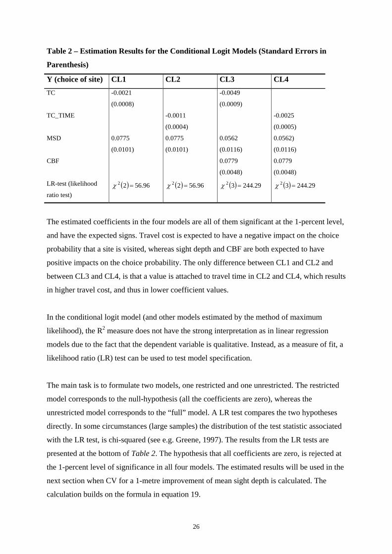
Table 2 – Estimation Results for the Conditional Logit Models (Standard Errors in

Parenthesis)

Y (choice of site) CL1 CL2 CL3 CL4

TC

TC_TIME

MSD

CBF

LR-test (likelihood

ratio test)

-0.0021

(0.0008)

0.0775

(0.0101)

( ) 96.5622 =χ

-0.0011

(0.0004)

0.0775

(0.0101)

( ) 96.5622 =χ

-0.0049

(0.0009)

0.0562

(0.0116)

0.0779

(0.0048)

( ) 29.24432 =χ

-0.0025

(0.0005)

0.0562)

(0.0116)

0.0779

(0.0048)

( ) 29.24432 =χ

The estimated coefficients in the four models are all of them significant at the 1-percent level,

and have the expected signs. Travel cost is expected to have a negative impact on the choice

probability that a site is visited, whereas sight depth and CBF are both expected to have

positive impacts on the choice probability. The only difference between CL1 and CL2 and

between CL3 and CL4, is that a value is attached to travel time in CL2 and CL4, which results

in higher travel cost, and thus in lower coefficient values.

In the conditional logit model (and other models estimated by the method of maximum

likelihood), the R2 measure does not have the strong interpretation as in linear regression

models due to the fact that the dependent variable is qualitative. Instead, as a measure of fit, a

likelihood ratio (LR) test can be used to test model specification.

The main task is to formulate two models, one restricted and one unrestricted. The restricted

model corresponds to the null-hypothesis (all the coefficients are zero), whereas the

unrestricted model corresponds to the “full” model. A LR test compares the two hypotheses

directly. In some circumstances (large samples) the distribution of the test statistic associated

with the LR test, is chi-squared (see e.g. Greene, 1997). The results from the LR tests are

presented at the bottom of Table 2. The hypothesis that all coefficients are zero, is rejected at

the 1-percent level of significance in all four models. The estimated results will be used in the

next section when CV for a 1-metre improvement of mean sight depth is calculated. The

calculation builds on the formula in equation 19.

26

4.4 A Policy Experiment

As a policy experiment, a 1-metre improvement of mean sight depth in the archipelago is

simulated. Approximately this corresponds to a 30 percent reduction of the nutrient

concentration. The results above reflect the actual level of water quality, but we are interested

in the value of improved water quality. Equation 19 states that we need to know the difference

between the indirect utility function corresponding to improved water quality, and the indirect

utility function of unchanged water quality.

A variable for improved mean sight depth is constructed by adding 1 metre to original mean

sight depth. The two indirect utility functions, for actual and improved sight depth, are

summed over the whole sample. Then the logarithm of the difference between the two sums is

divided by the marginal utility of income, which Hanemann (1984) has shown is the negative

of the coefficient of travel cost. This produces an estimate of compensating variation per trip.

Table 3 presents the estimated aggregated consumer surpluses of the two counties Stockholm

and Uppsala for 1998, 1999 and an average of these two years.

Table 3 – Aggregated Consumer Surplus (million SEK)

CL1 CL2 CL3 CL4

CV (1998)

CV (1999)

CV (average)

111

170

140

215

330

273

35

53

44

67

103

85

As expected, the consumer surplus is higher when time is valued. Again, weather conditions

in the summer of 1998 were very poor, and thus the figures of consumer surplus for this year

should be interpreted as lower bound estimates. In the same manner, the estimates for 1999

can be interpreted as upper bound estimates due to the extraordinary beautiful weather in the

Stockholm region that summer. Hence, a normal summer the recreational benefits should lie

somewhere between these extreme bounds, SEK 85-273 million when travel time is valued

and 44-140 when it is not. However, since it is strongly recommended to value time in

recreation demand models, the estimations that exclude travel time are not further interpreted

in this paper. From Table 3 it is also evident that benefits fall significantly when the

communication variable enters the model.

27

5 Conclusions

The recreational benefits from improved water quality in the Stockholm archipelago are

estimated in this paper. With the conditional logit model the aggregated consumer surplus is

estimated as SEK 85-273 million a normal summer, depending on whether or not a

communication variable is included.

These figures are lower than those of Sandström (1996). With the conditional logit model he

estimated the consumer surplus from a 50 percent reduction of the nutrient load to SEK 330

million for the entire Swedish coast per year. Apparently Sandström regarded both a larger

population and a greater improvement of water quality, which may explain the difference

between the two studies. Sandström’s figures should be interpreted as lower bound estimates

since a large fraction of trips are not included in his data set. In the Tourism and Travel

Database (TDB) that Sandström used are only overnight trips and day trips to destinations

situated no less than 100 kilometres away from home included.15 A large fraction of trips –

daytrips and overnight trips situated less than 100 kilometres from home - are thus excluded

from the study. Many of these trips should be covered by the present study. The consumer

surplus of the present study is still likely to be biased downwards due to the fact that trips

from outside Stockholm and Uppsala are not included.

One potential problem is the small number of explanatory variables in the model. The

problem of endogeneity when adding attraction variables makes it difficult to find suitable

variables. It is evident that consumer surplus falls considerably when the communication

variable enters the model. This fact, if nothing else, emphasises the importance to include

exogenous explanatory variables in the conditional logit model since the results may be quite

dramatically changed when we do so. Further, by adjusting the travel costs according to the

respondents’ purposes with their trips, the risk of exaggerating the economic value of

improved water quality has been reduced.

This paper does not have the ambition to conduct CBA on improved water quality, although it

is interesting indeed to compare the benefit measure obtained here with some recent estimates

of the costs for reduced nutrient concentration in the same region. Recent estimations

28

(Scharin, 2005) indicate that the cost for a 30 percent reduction of the nutrient concentration

is SEK 57 million per year.16 Based on the average welfare estimates for 1998 and 1999 (SEK

85-273 million), there would be a net benefit of SEK 28-216 million a year to society from a

reduction of the nutrient concentration in the archipelago.

The recreational benefits of this study are considerably lower than the possibly total benefits

that Söderqvist and Scharin (2000) estimated by using the contingent valuation method

(CVM) on reduced eutrophication in the Stockholm archipelago. This is not surprising, since

the TCM measures only use-values whereas the CVM aims at including non-use values too.

The difference between the two studies can possibly be explained by the presence of non-use

values in the latter study. The estimated benefits by the CVM study for the population of

Stockholm and Uppsala is SEK 506-842 million per year.

15 The TDB is based on 2000 (4000 in June and July) telephone interviews each month on travel behaviour. 16 The percentage approximately corresponds to a 1-metre improvement of sight depth.

29

References

Becker, G.S., (1965), “A Theory of the Allocation of Time”, The Economic Journal, 75: 493-517. Bockstael, N.E., Hanemann, W.M., Strand, I.E., (1987), Measuring the Benefits of Water Quality Improvements Using Recreation Demand Models, Volume II, Report to US EPA, Department of Agricultural and Resource Economics, University of Maryland. Bockstael, N.E., McConnell, K.E., Strand, I.E., (1991) in J.B. Braden and C.D. Kolstad, eds. Measuring the demand for environmental quality, North-Holland, Amsterdam, New York, Oxford and Tokyo. Bockstael, N.E., McConnell, K.E., (1993), “Public goods as quality characteristics of non-market commodities”, The Economic Journal, 103:1244-1257. Bojö, J.,(1985), “Kostnadsnyttoanalys av fjällnära skogar: fallet Vålådalen”, Research Report, Stockholm School of Economics, Dep. Of Economics. Boonstra, F., (1993), “Valuation of Ski Recreation in Sweden: A Travel Cost Analysis”, Umeå Economic Studies No. 316, University of Umeå. Cesario, F.J.,(1976), “Value of Time in Recreation Benefit Studies”, Land Economics, 52:1:32-41. Clawson, M., and Knetsch, J.L., (1966), Economics of Outdoor Recreation, Resources for the Future, Washington D.C. Cronin and Herzeg, (1982), “Valuing Nonmarket Goods Through Contingent Markets”, Report No. PNL-4255, Richland, WA: Pacific Northwest Laboratory. Daily, G.C., Söderqvist, T., Aniyar, S., et al (2000), “The Value of Nature and the Nature of Value”, Science, 289:395-396. Daubert and Young, (1981), “Recreational Demands for Maintaining Instream Flows: A Contingent Valuation Approach, American Journal of Agricultural Economics, 63:666-676. DeSerpa, A.C., (1971), “A Theory of the Economics of Time”, The Economic Journal, Dec 1971:828-846. Diamond, P.A., and Hausmann, J.A., (1994), “Contingent Valuation: Is Some Number Better than No Number?”, Journal of Economic Perspectives, 8:4:45-64. Freeman, A.M., (1979), “The benefits of air and water pollution: A review and synthesis of recent estimates”, Technical report prepared for the Council on Environmental Quality, Washington, D.C.

30

Gravelle, H., Rees, R., (1998), Microeconomics, Longman, London and New York. Greene, W.H., (1997), Econometric Analysis, Prentice-Hall Int. Inc., London. Haab, T.C., Hicks, R.L., (1999), ”Choice Set Considerations in Models of Recreation Demand”, Marine Resource Economics, 14: 4:271-281. Hanemann, W.M, (1982), “Applied welfare analysis with qualitative response models”, Working paper, no 241, California Agricultural Experiment Station, Division of Agricultural Sciences, University of California, Berkeley. Hanemann, W.M., (1984), “Welfare Analysis with Discrete Choice Models”, Working Paper, Department of Agricultural and Resource Economics, University of California, Berkeley. Hanemann, W.M., (1994), “Valuing the Environment Through Contingent Valuation”, Journal of Economic Perspectives, 8:4:19-43. Heckman, J.J, (1974), “Shadow Prices, Market Wages, and Labor Supply”, Econometrica, 42:679-694. Hotelling, H., (1948), Letter to the U.S. National Park Service. Maddala, G.S., (1983), Limited-Dependent and Qualitative Variables in Econometrics, New York, Cambridge University Press. McFadden, D., (1973), Conditional Logit Analysis of Qualitative Choice Behavior, in Zarembka, P., ed, Frontiers in Econometrics, Academic Press, New York. Mäler, K-G, (1974), Environmental Economics: a Theoretical Inquiry, John Hopkins University Press, Baltimore. Perman, R, Ma, Y, McGilvray, J and Common, M, (1999), Natural Resource and Environmental Economics, Longman, London, New York. Portney, P.R., (1994), “The Contingent Valuation Debate: Why Economists Should Care”, Journal of Economic Perspectives, 8:4:3-17. Sandström, M., Scharin, H., Söderqvist, T., (2000), “Seaside Recreation in the Stockholm Archipelago: Travel Patterns and Costs”, Discussion Paper, no. 129, Beijer International Institute of Ecological Economics, The Royal Swedish Academy of Sciences. Sandström, M.,(1996), “Recreational Benefits from Improved Water Quality: A Random Utility Model of Swedish Seaside Recreation”, Working paper no 121, Stockholm School of Economics, Working Paper Series in Economics and Finance. Scharin, H., (2004), ”Management of Eutrophicated Coastal Zones: The quest for an optimal policy under spatial heterogeneity”, Doctoral Thesis, Swedish University of Agricultural Sciences, Uppsala.

31

Small, K.A, and Rosen, H.S., (1981), “Applied welfare economics with discrete choice models, Econometrica, 49:1:105-130. SMHI Swedish Water Archive (SMHI, Svenskt Vattenarkiv, Havsområdesregister),(1993). Söderqvist, T. and Scharin, H, (2000), “The Regional Willingness to Pay for a Reduced Eutrophication in the Stockholm archipelago”, Discussion Paper, no. 128, Beijer International Institute of Ecological Economics, The Royal Swedish Academy of Sciences. Walsh, R.G., Greenley, D.G., Young, R.A., McKean, J.R. and Prato, A.A., (1978), “Option Values, Preservation Values and Recreational Benefits of Improved Water Quality: A Case Study of the South Platte River Basin, Colorado”, EPA-600/5-78-001, U.S. Environmental Protection Agency, Office of Research and Development. Willig, R.D.,(1976), “Consumer’s Surplus Without apology”, American Economic Review, 66:4:589-597. Sources of sight depth data, maps etc Haninge kommun, sight depth observations from Miljö & Stadsbyggnad, miljökontoret, “Utvärdering av vattenprovtagningar och analyser i några havsvikar i Haninge kommun 1992-1998”, Ulf Larsson at Akvatisk Miljöforskning AB. Himmerfjärden Eutrophication Study, http://www.ecology.su.se/dbhfj/hfjsmall.htm, Joakim Pansar. Inregia AB, Basemma Codes for Stockholm County and Maps with Basemma Zones. Inregia AB, Travel time- and distance matrix from the County Council (Landstinget) of Stockholm, traffic database Emma, Lars Pettersson. Lantmäteriet, (The National Land Survey of Sweden), “Blå kartan”, no. 96, 106 and 116. Naturvårdsverket (The Swedish Environmental Protection Agency), Britta Hedlund. Norrtälje kommun, sight depth observations from The County Administrative Board (Länsstyrelsen) of Stockholm, Joakim Pansar. Nynäshamn kommun, sight depth observations. Stockholm Vatten AB, sight depth observations for 1997, 1998 and 1999, Christer Lännergren. Sjöhistoriska museet (The National Maritime Museum of Sweden), Malin Joakimsson. Tyresö kommun, sight depth observations from Miljö- och stadsbyggnadsförvaltningen, planeringsavdelningen, Göran Eriksson.

32