The Value of Health and Longevity

Kevin M. Murphy Robert H. Topel University of Chicago University of Chicago

Revised March 15, 2005

Abstract

We develop an economic framework for valuing improvements to health and life expectancy, based on individuals’ willingness to pay. We then apply the framework to past and prospective reductions in mortality risks, both overall and for specific life-threatening diseases. We calculate (i) the social values of increased longevity for men and women over the 20th century; (ii) the social value of progress against various diseases after 1970; and (iii) the social value of potential future progress against various major categories of disease. The historical gains from increased longevity have been enormous. Over the 20th century, cumulative gains in life expectancy were worth over $1.2 million per person for both men and women. Between 1970 and 2000 increased longevity added about $3.2 trillion per year to national wealth, an uncounted value equal to about half of average annual GDP over the period. Reduced mortality from heart disease alone has increased the value of life by about $1.5 trillion per year since 1970. The potential gains from future innovations in health care are also extremely large. Even a modest 1 percent reduction in cancer mortality would be worth nearly $500 billion. The authors are also Research Associates of the National Bureau of Economic Research, Senior Fellows of the Milkin Institute, and Research Associates of the George J. Stigler Center for the Study of the Economy and the State. We acknowledge support from the Milken Foundation, the Lasker Charitable Trust, and the Stigler Center. An earlier version was presented as keynote lectures to the European meetings of the Econometric Society and the Society of Labor Economists, as the Thompson Lecture to the Midwest Economic Association, the Pihl Lecture at Wayne State University, and in workshops at the World Bank, the University of Chicago, Stanford University, Boston University, NBER, MIT, University of Wisconsin, and Texas A&M.

1

I. Introduction

During the 20th century, life expectancy at birth for a representative American increased by

roughly 30 years. In 1900, nearly 18 percent of males born in the United States died before their

first birthday – today, it isn’t until age 62 that cumulative mortality reaches 18 percent.1 As we

demonstrate below, this remarkable increase in longevity reflects progress against a variety of

afflictions and diseases, driving reductions in mortality at all ages. It illustrates a substantial, but

unmeasured, increase in social welfare due to improvements in health.

This paper develops and applies an economic framework for valuing improvements in

health and longevity, based on individuals’ willingness to pay. We use our framework to estimate

the economic gains from declining mortality in the United States over the 20th century, and to

value the prospective gains that could be obtained from further progress against major diseases.

We find that these values are enormous. Gains in life expectancy over the century were worth

over $1.2 million per person to the current population. From 1970 to 2000 gains in life

expectancy added about $3.2 trillion per year to national wealth, with half of these gains due to

progress against heart disease alone. Looking ahead, we estimate that even modest progress

against major diseases would be extremely valuable. For example, a permanent 1 percent

reduction in mortality from cancer has a present value to current and future generations of

Americans of nearly $500 billion, while a cure (if one is feasible) would be worth about $50

trillion.

1 Death rates by age are recorded in Vital Statistics of the United States. Other developed countries show similar progress over the century. Longer term data are scant, but suggest that progress accelerated up until about 1950. For example, Swedish data since 1751 show an increase in life expectancy of 6 years between 1800 and 1850, 9 years between 1850 and 1900, 17 years between 1900 and 1950, and 9 years between 1950 and 2000 (Statistics Sweden, Program for Population Statistics).

2

Our analysis of the values of health improvements is founded on individuals’

maximization of lifetime expected utility. We distinguish two types of health improvements –

those that extend life by reducing mortality, and those that raise the quality of life. Life extension

is valued because utility from goods and leisure accrues over a longer period, and improvements in

the quality of life raise utility from given amounts of goods and leisure. This framework delivers

precise expressions for the economic value of a life-year, for the value of remaining life, and for

changes in these values when health improves. We show that the social value of improvements in

health is greater: (a) the larger is the population, (b) the higher are average lifetime incomes, (c)

the greater is the existing level of health, and (d) the closer are the ages of the population to the

age of onset of disease. These factors point to an increasing valuation of health improvements

over the past several decades and into the future. As the U.S. population grows, as lifetime

incomes grow, as health levels improve and as the baby-boom generation approaches the primary

ages of disease-related death, the social value of improvements in health will continue to rise.

We also show that improvements in health tend to be complementary; for example,

improvements in life expectancy (from any source) raise willingness to pay for further health

improvements by increasing the value of remaining life. This means that advances against one

disease, say heart disease, raise the value of progress against other age-related ailments such as

cancer or Alzheimer’s. This is of significant empirical relevance, as it implies that the well-

documented historical progress against heart disease, for which mortality has fallen by roughly 30

percent since 1970, has increased the value of further progress against other afflictions. We find

that reductions in mortality since 1970 have raised the value of further health progress by about 18

percent.

3

An analysis of the social value of improvements in health is a first step toward evaluating

the social returns to medical research and health-augmenting innovations. Improvements in health

and longevity are partially determined by society’s stock of medical knowledge, for which basic

medical research is a key input. The U.S. invests over $50 billion annually in medical research, of

which about 40 percent is federally funded, accounting for 25 percent of government research and

development outlays.2 The $27 billion federal expenditure for health related research in FY 2003,

the vast majority of which is for the National Institutes of Health, represented a real dollar

doubling over 1993 outlays. Are these expenditures warranted? Our analysis suggests that the

returns to basic research may be quite large, so that substantially greater expenditures may be

worthwhile. By way of example, take our estimate that a 1 percent reduction in cancer mortality

would be worth about $500 billion. Then a “war on cancer” that would spend an additional $100

billion (over some period) on cancer research and treatment would be worthwhile if it has a 1-in-5

chance of reducing mortality by 1 percent, and a 4-in-5 chance of doing nothing at all.

Against these potential benefits of improving health one must weigh the costs of

implementing new medical technologies. Our analysis highlights some of the important economic

issues surrounding the valuation of improvements in health, health research and the growth in

health expenditures. Many of these issues have significant policy implications. For example, the

annuitization of many public and private retirement benefits (Social Security, private pensions,

Medicare and private medical coverage) and the prevalence of third party payers increase

incentives to spend on medical care, even when benefits are far smaller than costs. These

distortions also skew investments in research away from cost-decreasing improvements in

2 The distribution of health R&D expenditure is reported by the National Institutes of Health. See http://www.cdc.gov/nchs/products/pubs/pubd/hus/tables/2001/01hus126.pdf. Pharmaceutical industry R&D expenditures are reported in www.phrma.org/publications/publications/profile02/chapter2.pdf. Government

4

technology, as the demand for care is artificially price insensitive. This creates “second-best”

considerations in valuing medical advances: innovations that would otherwise be welfare

improving may be socially wasteful because ex-post utilization decisions are distorted. In the

presence of such distortions, we must take account of the induced effect that medical advances

have on expenditures when evaluating the social returns to improvements in technology. Our

methodology does this, and we provide evidence on the value of improving health relative to

increased health care expenditures. Overall, the value of increased longevity has greatly exceeded

the costs of health care, though for some cases we find negative net social values.

The paper is organized as follows. Section II provides some empirical foundation for the

analysis that follows, documenting the increase in longevity, and its sources, that occurred has

occurred in the U.S. Section III develops our economic model for valuing improvements in health

and life expectancy, and Sections IV calibrates willingness to pay for health improvements.

Sections V and VI present the empirical application of our methods, estimating the economic

gains associated with the improvements in life expectancy over the 20th century, with particular

focus on the post-1970 period. We also estimate the potential gains to future progress against

major categories of disease, and we provide a rough estimate of the value of improvements in the

health-related “quality” of life. Section VII concludes.

II. The Setting: Long-Term Evidence of Improvements in Health

Figure 1 shows life expectancy at birth and age 50 in the United States since 1900. These and

other estimates that follow are based on cross sectional age-specific death rates at each date, so

(when health is improving) they will underestimate life expectancy for a given birth cohort. The

figure shows that life expectancy over the century increased by slightly over 30 years. Progress

expenditures for health R&D are reported by the National Science Foundation; see www.nsf.gov/sbe/srs/nsf02330/historic.htm.

5

during the first half of the century was rapid and evidently concentrated at younger ages – life

expectancy conditional on reaching age 50 grew only slightly. In 1900, about 18 percent of males

died before their first birthday. By 1950 it took 52 years for cumulative male mortality to reach

18 percent, and with current mortality rates it would take 62 years. Progress slowed between 1950

and 1970, especially for men, but the upward trend in life expectancy began again after 1970.

Late century gains were especially prominent for older individuals—expected remaining life of 50

year old men has increased by 5 years since 1970.

Tables 1 and 2 provide further insight into the reasons for these trends. Table 1 uses age

specific mortality data to decompose inter-decade changes in longevity into contributions from

various age intervals. The estimates show the additional life years contributed by declining

mortality rates in each age interval and decade; for example, between 1910 and 1920 lower male

infant mortality (<1 year old) contributed 2.48 of the 4.85 expected life-years gained over the

decade. The table demonstrates important age and gender differences in the timing of life-

extending improvements in health. Over the century reductions in infant (<1) and child (1-14)

mortality were the major contributing factors to increasing lifespans, yet almost all (85%) of these

gains occurred before 1950. This partially explains the slowdown in overall growth that occurred

from 1950 to 1970. In contrast, the renewal of growth that occurred after 1970 is largely

accounted for by declining mortality among older Americans. For example, the contribution of

reduced mortality among men aged 55 and over was negligible before 1970, but since then

declining death rates of older men have added 3.9 years to expected lifetimes. This is more than

half of the total male gain over that period. Women’s gains at older ages began earlier, in the

1940’s, but slowed relative to men’s gains after 1980.3

3 Evidence for other developed countries roughly conforms to the data in Figure 1 and Tables 1 and 2. For OECD countries as a whole, from 1960 to 2000 the average at-birth life expectancy of women increased by 9 years and that

6

This shift in the age distribution of rising longevity reflects differential progress against life-

threatening ailments, shown in Table 2. The importance of declining mortality from afflictions

that strike older individuals is clear. Since 1950 the largest single contributor is reduced mortality

from heart disease, which added more than 3.5 years to the expected lifetimes of both men and

women, accounting for more than 40 percent of the total. When combined with strokes, progress

against cardiovascular diseases added 4.7 and 5.1 years to the expected lifetimes of men and

women, with most of the gain occurring after 1970.4

These data are the foundation for the problem we study. Rising longevity, and health

improvements more generally, are a form of economic progress. Valuation of these gains is

important for two reasons. First, traditional measures of economic growth and welfare, based on

national income accounts, make no attempt to account for this source of rising living standards.

They therefore underestimate improvements in well-being. Second, public expenditure accounts

for a large portion of both medical research and the provision of medical care. Efficient decisions

require a framework for measuring the value of treatment, and of research-based medical progress.

III. Economic Framework: Valuing Improvements in Health

Advances in health-related knowledge and its application can take many forms, ranging

from the development of new medicines and techniques for treating disease to improvements in

public health infrastructure. These advances affect the quality of life and the risks of mortality at

various stages of the lifecycle. We assume that these effects are channeled through the intangible

“health” of individuals, of which we distinguish two types. The first, H(t), raises the quality of life

of men by 8 years. OECD Health Data, Table 1, Life Expectancy in Years, http://www.oecd.org/xls/M00031000/M00031357.xls. 4 These tabulations indicate little progress against cancer. This is partly an artifact of the way the underlying data are aggregated. Closer examination (we do not provide the details here) shows declining cancer mortality at younger ages and rising mortality at older ones, with the overall age-adjusted rate fairly constant. This may reflect selection: those who would have died from heart disease at younger ages may also be more prone to die from cancer later in life.

7

without affecting mortality. For example, new medicines that improve mental health, cure

migraine headaches, or reduce the effects of arthritis will increase instantaneous utility without

necessarily affecting the length of life. The other, G(t), affects mortality without affecting the

quality of life. New methods of detecting treatable diseases or advances in surgical techniques are

examples. Of course, many advances in medical knowledge affect both types of health. New

medicines that reduce blood pressure or retard the advance of cancer can raise both the quality of

life and its duration. H(t) and G(t) are affected by the state of health technologies and also by

individuals’ choices, but we relegate these choices to the background.

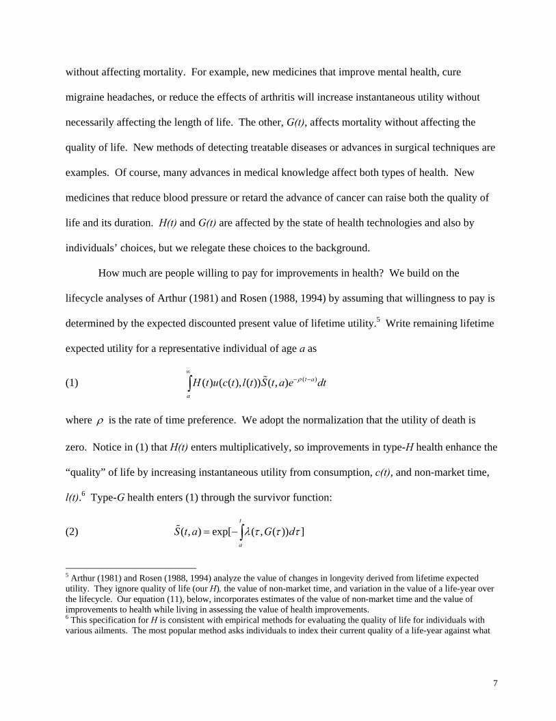
How much are people willing to pay for improvements in health? We build on the

lifecycle analyses of Arthur (1981) and Rosen (1988, 1994) by assuming that willingness to pay is

determined by the expected discounted present value of lifetime utility.5 Write remaining lifetime

expected utility for a representative individual of age a as

(1) ( )( ) ( ( ), ( )) ( , ) t a

a

H t u c t l t S t a e dtρ∞

− −∫ %

where ρ is the rate of time preference. We adopt the normalization that the utility of death is

zero. Notice in (1) that H(t) enters multiplicatively, so improvements in type-H health enhance the

“quality” of life by increasing instantaneous utility from consumption, c(t), and non-market time,

l(t).6 Type-G health enters (1) through the survivor function:

(2) ( , ) exp[ ( , ( )) ]t

a

S t a G dλ τ τ τ= −∫%

5 Arthur (1981) and Rosen (1988, 1994) analyze the value of changes in longevity derived from lifetime expected utility. They ignore quality of life (our H), the value of non-market time, and variation in the value of a life-year over the lifecycle. Our equation (11), below, incorporates estimates of the value of non-market time and the value of improvements to health while living in assessing the value of health improvements. 6 This specification for H is consistent with empirical methods for evaluating the quality of life for individuals with various ailments. The most popular method asks individuals to index their current quality of a life-year against what

8

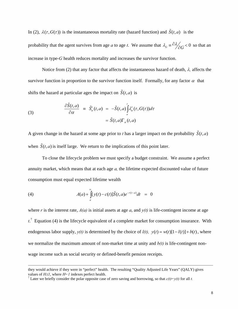
In (2), ( , ( ))Gλ τ τ is the instantaneous mortality rate (hazard function) and ( , )S t a% is the

probability that the agent survives from age a to age t. We assume that 0G Gλλ ∂≡ <∂ so that an

increase in type-G health reduces mortality and increases the survivor function.

Notice from (2) that any factor that affects the instantaneous hazard of death, λ, affects the

survivor function in proportion to the survivor function itself. Formally, for any factor α that

shifts the hazard at particular ages the impact on ( , )S t a% is

(3) ( , ) ( , ) ( , ) ( , ( ))

( , ) ( , )

t

a

S t a S t a S t a G d

S t a t a

α α

α

λ τ τ τα

∂ ′ ′≡ = −∂

= Γ

∫%

% %

%

A given change in the hazard at some age prior to t has a larger impact on the probability ( , )S t a%

when ( , )S t a% is itself large. We return to the implications of this point later.

To close the lifecycle problem we must specify a budget constraint. We assume a perfect

annuity market, which means that at each age a, the lifetime expected discounted value of future

consumption must equal expected lifetime wealth

(4) ( )( ) [ ( ) ( )] ( , ) 0r t a

a

A a y t c t S t a e dt∞

− −+ − =∫ %

where r is the interest rate, A(a) is initial assets at age a, and y(t) is life-contingent income at age

t.7 Equation (4) is the lifecycle equivalent of a complete market for consumption insurance. With

endogenous labor supply, y(t) is determined by the choice of l(t), ( ) ( )[1 ( )] ( )y t w t l t b t= − + , where

we normalize the maximum amount of non-market time at unity and b(t) is life-contingent non-

wage income such as social security or defined-benefit pension receipts.

they would achieve if they were in “perfect” health. The resulting “Quality Adjusted Life Years” (QALY) gives values of H≤1, where H=1 indexes perfect health. 7 Later we briefly consider the polar opposite case of zero saving and borrowing, so that c(t)=y(t) for all t.

9

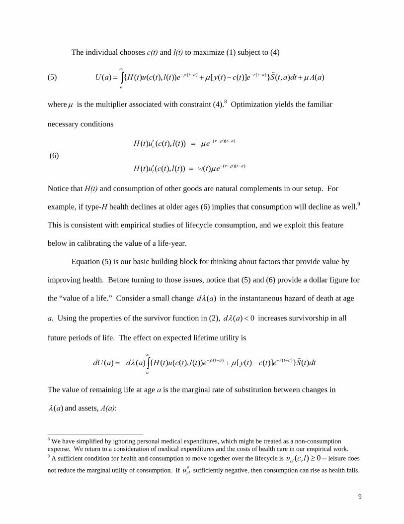
The individual chooses c(t) and l(t) to maximize (1) subject to (4)

(5) ( ) ( )( ) { ( ) ( ( ), ( )) [ ( ) ( )] } ( , ) ( )t a r t a

a

U a H t u c t l t e y t c t e S t a dt A aρ µ µ∞

− − − −= + − +∫ %

whereµ is the multiplier associated with constraint (4).8 Optimization yields the familiar

necessary conditions

(6)

( )( )

( )( )

( ) ( ( ), ( ))

( ) ( ( ), ( )) ( )

r t ac

r t al

H t u c t l t e

H t u c t l t w t e

ρ

ρ

µ

µ

− − −

− − −

′ =

′ =

Notice that H(t) and consumption of other goods are natural complements in our setup. For

example, if type-H health declines at older ages (6) implies that consumption will decline as well.9

This is consistent with empirical studies of lifecycle consumption, and we exploit this feature

below in calibrating the value of a life-year.

Equation (5) is our basic building block for thinking about factors that provide value by

improving health. Before turning to those issues, notice that (5) and (6) provide a dollar figure for

the “value of a life.” Consider a small change ( )d aλ in the instantaneous hazard of death at age

a. Using the properties of the survivor function in (2), ( ) 0d aλ < increases survivorship in all

future periods of life. The effect on expected lifetime utility is

( ) ( )( ) ( ) { ( ) ( ( ), ( )) [ ( ) ( )] } ( )t a r t a

a

dU a d a H t u c t l t e y t c t e S t dtρλ µ∞

− − − −= − + −∫ %

The value of remaining life at age a is the marginal rate of substitution between changes in

( )aλ and assets, A(a):

8 We have simplified by ignoring personal medical expenditures, which might be treated as a non-consumption expense. We return to a consideration of medical expenditures and the costs of health care in our empirical work. 9 A sufficient condition for health and consumption to move together over the lifecycle is ( , ) 0clu c l ≥ -- leisure does

not reduce the marginal utility of consumption. If clu′′ sufficiently negative, then consumption can rise as health falls.

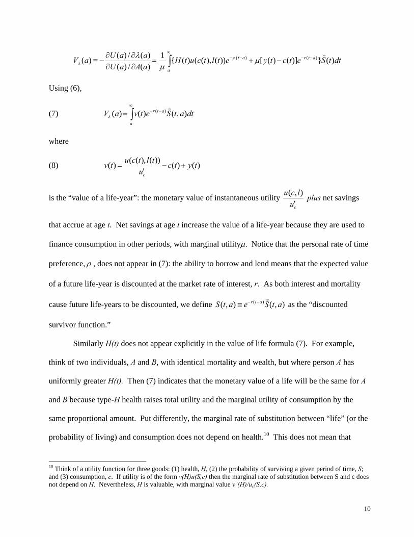
10

( ) ( )( ) / ( ) 1( ) { ( ) ( ( ), ( )) [ ( ) ( )] } ( )( ) / ( )

t a r t a

a

U a aV a H t u c t l t e y t c t e S t dtU a A a

ρλ

λ µµ

∞− − − −∂ ∂

≡ − = + −∂ ∂ ∫ %

Using (6),

(7) ( )( ) ( ) ( , )r t a

a

V a v t e S t a dtλ

∞− −= ∫ %

where

(8) ( ( ), ( ))( ) ( ) ( )c

u c t l tv t c t y tu

= − +′

is the “value of a life-year”: the monetary value of instantaneous utility ( , )

c

u c lu′

plus net savings

that accrue at age t. Net savings at age t increase the value of a life-year because they are used to

finance consumption in other periods, with marginal utilityµ. Notice that the personal rate of time

preference, ρ , does not appear in (7): the ability to borrow and lend means that the expected value

of a future life-year is discounted at the market rate of interest, r. As both interest and mortality

cause future life-years to be discounted, we define ( )( , ) ( , )r t aS t a e S t a− −≡ % as the “discounted

survivor function.”

Similarly H(t) does not appear explicitly in the value of life formula (7). For example,

think of two individuals, A and B, with identical mortality and wealth, but where person A has

uniformly greater H(t). Then (7) indicates that the monetary value of a life will be the same for A

and B because type-H health raises total utility and the marginal utility of consumption by the

same proportional amount. Put differently, the marginal rate of substitution between “life” (or the

probability of living) and consumption does not depend on health.10 This does not mean that

10 Think of a utility function for three goods: (1) health, H, (2) the probability of surviving a given period of time, S; and (3) consumption, c. If utility is of the form v(H)u(S,c) then the marginal rate of substitution between S and c does not depend on H. Nevertheless, H is valuable, with marginal value v’(H)/uc(S,c).

11

health has no value, however; it simply says that willingness to pay for changes in survival do not

depend on the level of health. This property is consistent with empirical evidence, as summarized

by the Environmental Protection Agency’s Science Advisory Board (2000):

There are no published studies that show that persons with physical limitations or chronic illnesses are willing to pay less to increase their longevity than persons without those limitations. People with physical limitations appear to adjust to their conditions, and their willingness to pay to reduce fatal risks is therefore not affected.11

Life-Cycle Changes in the Value of Life

While differences in type-H health between individuals do not generate corresponding

differences in the value of life, age-related changes in type-H health and income affect the age

profile of the value of a life-year. Adopting the notation log ( ) /x d x t dt•

≡ , differentiation of (8)

yields the rate of change in the value of a life-year as an individual ages:

(9) ( ) ( ) ( )( ) ( ) ( ) (1 ( )) ( ) 1 ( )( ) ( )w w

y t y t c tv t s t w t s t b t H t rv t v t

ρ• • • •⎛ ⎞−⎛ ⎞ ⎛ ⎞= + − + − + −⎜ ⎟ ⎜ ⎟⎜ ⎟⎝ ⎠ ⎝ ⎠⎝ ⎠

where sw is the share of labor earnings in total life-contingent income. The first term in (9) ties the

age profile of v(t) to changes in income. Pre-retirement we can set sw=1, so the value of a life-year

tracks the age profile of wages. Indexing of post-retirement annuity incomes suggests b•

=0 is a

good approximation for retired persons. The second term ties life-cycle changes in v(t) to changes

in health and to time preference. Complementarity between type-H health and consumption of

goods and leisure in (6) causes the value of a life-year to fall as health declines ( 0H•

< ) at older

ages, so persons with declining health are, in effect, more impatient. In our later empirical work

we calibrate a lifecycle pattern of H•

based on lifecycle patterns of consumption.

11 http://www.epa.gov/sab/pdf/eeacf013.pdf

12

Cost-benefit evaluations that apply employ empirical estimates of the “value of a

statistical” life (VSL), and the empirical studies on which they are founded, typically assume that

VSLs do not depend on age. Then it is just as valuable to “save” a 60 year old as a 40 year old.

Our framework indicates that the value of remaining life is age dependent, first rising and then

falling as a person ages. From (7) the value of remaining life satisfies the usual law of motion for

an asset price:

( ) ( ( )) ( ) ( )V a r a V a v aaλ

λλ∂= + −

∂

Letting R(a) represent the (discounted) length of remaining life at age a, this becomes

(10) [ ]( ) ( )( ( )) ( ) ( ) ( , ) ( )a

V a R ar a v t v a S t a dt v aa aλ λ

∞∂ ∂= + − +

∂ ∂∫

Life tables for the United States and other developed economies indicate that the last term is

negative at all ages—surviving another year reduces the length of remaining life—though it is

conceivably positive in situations where the young are at particularly high risk of death, say due to

childhood disease or violence. The first term is positive (negative) if the future is “better” (worse),

on average, than the present. From (9), this term will be positive at younger ages because wages

typically rise with age and because type-H health is unlikely to deteriorate much among the young.

Later in life, when wage growth is negligible, ( )V aλ must decline as persons age because type-H

health deteriorates ( ( ) ( )v t v a< for t > a) and because the remaining length of life is falling.

Willingness to Pay for Improvements in Health

To see how this framework can be used to evaluate improvements in health, consider some

factor,α , that can affect both the type-H and type-G concepts of health. For purposes of

subsequent discussion we will refer toα as the state of “medical knowledge”—techniques,

medicines, and so on—though it can equally represent factors that improve public health, such as

13

environmental improvements, improved nutrition or access to medical care. The marginal value

of some improvement in medical knowledge follows from the displacement of (5):

(11) ( ) ( ) ( ( ), ( ))( ) ( ) ( , ) ( , ) ( , )( ) ca a

U a H t u c t l tV a v t S t a t a dt S t a dtH t u

α αα αµ

∞ ∞′ ′≡ = Γ +∫ ∫

Equation (11) measures the change in value of life induced by changes in any factor that affects

type-H or type-G health. The first term in (11) is the dollar value of the gain in lifetime expected

utility from changes in mortality, indexed by changes in the survivor

function ( , )( , ) ( , ) S t aS t a t aα α∂

Γ =∂

. These changes in the probability of survival weight the value

of a life-year in each period where mortality changes.

The second term is the value of changes in type-H health at each age, ( ) ( ) /H t H tα α′ ≡ ∂ ∂ ,

that raise quality of life while holding mortality fixed. These improvements weight utility itself,

with no contribution from net savings. Notice that when savings are negligible, proportional

changes in type-H health ( /H Hα′ ) and in the survivor function ( αΓ ) are valued in exactly the

same way. Living a bit better is like living a bit longer.

Equation (11) is the foundation for our efforts to value past and prospective changes in

longevity and the quality of life. To make empirical headway we restrict utility to be homothetic,

so ( , ) ( ( , ))u c l u z c l≡ where z is homogeneous of degree one. Then the dollar value of a life-year is

(suppressing time arguments)

(12) ( )( , )( , ) ( )

c l

c c

u z c z lu c lv y c y cu c l z u z

+= + − = + −

′

so z is a composite commodity that aggregates consumption and non-market time. Define full

consumption and full income by adding the shadow value of non-market time to consumption and

income:

14

1F lc

c

F l

c

zc c l z zzzy y lz

−= + =

= +

where for labor force participants we know that ( )( )

l l

c c

u z z wu z z

= = , the market wage. Then

( ) ( ) 1( ) ( )

F Fc l

c

u z c z l u zv y c y cz u z zu z

⎛ ⎞+= + − = + −⎜ ⎟′ ′⎝ ⎠

or

(13) ( )F Fv y c z= + Φ

In (13), ( )zΦ is consumer surplus per unit of the composite commodity z, which is identical to

surplus per dollar of full consumption. It is positive when average utility of z is greater than

marginal utility, or equivalently when the elasticity of utility with respect to z is smaller than 1.0.

The theory does not imply that ( )zΦ ≥ 0, however. Positive utility may require composite

consumption above some minimum subsistence level, 0z , where 0( ) 0u z = . Then 0( ) 1zΦ = − and,

by monotonicity of surplus, there is a 1 0z z> where 1( ) 0zΦ = .12

Equation (13) demonstrates two important points about the value of a life-year. First, even

if ( ) 0zΦ = the value of being alive exceeds measured income because of the value of non-market

time. This is especially important for persons without wage and salary income—such as the

retired—for whom the value of non-market time accounts for most of Fy . For full-time workers

non-working hours are valued at w and annual hours of leisure are (reasonably) greater than hours

worked, so that Fy may be more than double money income. Second, full consumption adds to

12 Note that v(t)<0 doesn’t mean that death is preferred, as the value of continued life at a is determined by

( )V aλ which will be positive if future prospects are brighter.

15

this value so long as ( ) 0zΦ > . For example, if ( ) 1zΦ = (surplus equals consumption expenditure)

and y=c (no savings), then the value of a life year would be more than 4 times annual income. For

a typical male at peak lifecycle earnings—roughly $45,000 per year around age 50—this would

put the value of a life year above $180,000. The evidence we develop below suggests it is larger

still.

Now use (13) to rewrite (7) and (11):

(14) ( ) [ ( ) ( ) ( ( ))] ( , )F F

a

V a y t c t z t S t a dtλ

∞

= + Φ∫

(15) ( )( ) [ ( ) ( ) ( ( ))] ( , ) ( , ) ( )[1 ( ( ))] ( , )( )

F F F

a a

H tV a y t c t z t S t a t a dt c t z t S t a dtH tα

α α

∞ ∞ ′= + Φ Γ + +Φ∫ ∫

Equation (14) is the value of an age-a statistical life, which is the expected discounted value of full

income and surplus on full consumption. Equation (15) is the age-a willingness to pay for

improvements in health. Both are proportional to full income and consumption, implying that

health is perhaps the ultimate “normal” good. To pursue this point let ( )( )( )

u zzzu z

σ′

= −′′

denote the

elasticity of intertemporal substitution (EIS) in consumption, and consider the impact of increased

income or wealth on v(t). Abstracting from saving by setting y=c, the income elasticity of v(t) is

(16) 1

log 1 11log ( ) 1 ( )

vy z zσ −

∂= + −

∂ +Φ

which is larger than 1.0 if 1( ) 1( )

zz

σ < +Φ

. Evidence developed below indicates ( )zΦ ≈ 2 for

prime-aged individuals, and empirical estimates of the EIS suggests ( ) 1.0zσ = as a rough upper

bound, so the condition is likely satisfied—with these values the income elasticity of the value of a

16

life year is 1.33. It would be larger still for values of ( ) 1.0zσ < , as are common found in

empirical applications.13

Equations (14)-(16) have a number of implications for valuing improvements in health and

health-related investments.

1. Willingness to pay for improvements in health is proportional to full income and full

consumption, so willingness to pay rises with wealth. That wealthier individuals are willing to

pay more for improvements in health may seem obvious, but the broader implication is that

economic growth is a boon to health-related investments. This is especially important when

willingness to pay for health improvements is income elastic, as suggested by (16). Then

richer societies invest proportionally more in health because life itself is more valuable.14

2. The relevant concepts of income and consumption include the shadow value of non-market

time. Common attempts to value life-years based on income or consumption expenditures

alone will miss a large part of what people value, especially when health improvements are

concentrated at older ages.15

3. Wealth constant, improvements in both type-G and type-H health are more valuable when

surplus per dollar of full consumption,Φ , is large. Intuitively,Φ is large when the demand

for current consumption is inelastic, so that consumption expenditures at different ages are

poor substitutes— ( )zσ is small. Then loss of a year of life cannot be offset by simply

reallocating consumption to other years. We exploit this notion in the next section, gauging

Φ from evidence on intertemporal substitution in consumption.

4. For given profiles of income and consumption, the value of a reduction in mortality ( αΓ ) or an

improvement in the quality of life ( /H Hα′ ) is larger when ( , )S t a is large. This suggests a

form of increasing returns in health improvements: medical and other advances that reduce

mortality raise the value of further advances, because individuals are more likely to be alive to

enjoy the benefits. So health-related investments will be more valuable to already healthy

13 Section IV discusses empirical evidence on ( )zσ . 14 Our estimates of the value of a life year are based on empirical estimates of the value of a statistical life (VSL), as surveyed in Viscusi (1992) and Viscusi and Aldy (2003). Based on comparisons of VSLs across countries Viscusi and Aldy conclude that the income elasticity of the value of a statistical life is about 0.6. 15 For example, the Conference Board of Canada’s (2001) estimates the “costs” of excess mortality based on what a decedent would have produced, not the value to the individual of remaining alive.

17

individuals, and in societies where average health is already high. We develop this point more

completely in Section V.

5. The value of progress against a particular disease is greatest when the current age, a, is close

to, but before, the typical age of onset of the disease. For example, for an ailment like

cardiovascular disease, mortality-reducing progress ( αΓ ) is likely to be concentrated at ages

50 and above. Then the expected present value of such progress will be greater at age 45 than

at ages 25 or 90 because of both discounting and survivorship. Thus we estimate in Section

VI that a 10% reduction in mortality from heart disease would be worth about $30,000 to a 45-

year old male but only about $15,000 to men aged 25 or 90. Similarly, progress against

Alzheimer’s that improves the quality of life ( /H Hα′ >0) will be more valuable to 60 year-olds

than to 30 year-olds.

IV. Calibration: The Value of a Life-Year

Our calibration strategy begins with estimates of “the value of a statistical life” taken from

the literature on willingness to pay for reductions in risks of accidental death (see Viscusi (1992)

for a survey or Thaler and Rosen (1975) for an original analysis). These studies estimate

willingness to pay from wage differences on jobs with varying probabilities of accidental death, or

from market prices for products (such as airbags) that reduce the likelihood of a fatal injury. For

example, suppose that workers in a particular occupation require a $500 annual wage premium in

order to accept a 1 in 10,000 increase in the annual probability of accidental death. In a population

of 10,000 workers this change in risk would raise expected deaths by 1 each year, with an

aggregate value of $500 × 10,000 = $5 million. Then the value of one statistical life is $5 million.

In our framework this is the conceptual equivalent of the value of remaining life given by ( )V aλ in

(14).

According to Viscusi’s (1993) survey, this literature yields a “reasonable range” of values

for ( )V aλ of $4 million to $9 million per statistical life, expressed in current (2004) dollars, while

18

Viscusi and Aldy (2003) provide a tighter range for U.S. data at $5.5 to $7.5 million. Government

agencies and panels regularly update these estimates to account for economic growth, new

methods, and evidence; for example since 1999 the Environmental Protection Agency used a value

of $6.3 million per statistical life in its cost-benefit analyses.16 These estimates are typically

founded on regression analyses of risk-income tradeoffs for working-age individuals, so for the

calculations that follow we will assume that the survivorship-weighted average value of a

statistical life for individuals between the ages of 25 and 55 is $6.3 million. Readers who prefer a

different value may adjust things accordingly, as most of our later estimates are scalable.

Given this average value in (14), it remains to impute a lifecycle shape for the value of a

life-year, ( ) ( ) ( ) ( ( ))F Fv t y t c t z t= + Φ , which in turn determines the lifecycle pattern of the value of

a life (14) and willingness to pay for health improvements (15). We construct v(t) from the

model’s structure and empirical evidence on key parameters. Values of full income ( )Fy t for a

representative individual can be constructed from lifecycle wage profiles, while the time paths of

( )c t and ( )Fc t satisfy

(17a) ( ) ( ) Lc r H s wσ ρ σ η σ= − + − −&& &

(17b) ( ) (1 )FLc r H s wσ ρ σ σ= − + − −&& &

where Ls is the share of non-market time in full consumption and η is the elasticity of substitution

between consumption and leisure in z(c,l). We assume that σ and η are constants, which implies

that z(c.l) is CES and that

(18) 1 1

11 1

10 01

1( ) ( ) 1 ( )1 1

z z zu z zz

σ σσσ

σ σ

− −

−− −

−−

− ⎛ ⎞= ⇒ Φ = −⎜ ⎟− − ⎝ ⎠

16 See Dockins et. al. (2004) for a review.

19

where 0( )u z =0. The value of a life-year will be larger when demand for current full consumption

is more inelastic, which occurs when there is little intertemporal substitution in consumption.

There is a substantial empirical literature seeking to estimate σ based on versions of (17a).

Hansen and Singleton (1983), Hall (1988), and Campbell and Mankiw (1989) find that aggregate

consumption growth is insensitive to changes in the real interest rate, so that σ is close to zero.

This would imply unreasonably large values of a life-year because ( )zΦ would be huge.

Similarly Barsky et. al. (1997), using questionnaire responses, find an upper bound on σ of about

0.36. In contrast, Browning, Hansen, and Heckman (1999) survey estimates of σ from micro-

data and conclude that the evidence favors a value for σ that is “a bit” larger than 1.0. We know

of no formal evidence on an analogue of 0 /z z , though comparisons of living standards over time

and across countries suggest that it is quite small. In effect, the ratio asks how much composite

consumption individuals would sacrifice before they would rather be dead. Notice that this ratio

must be sufficiently positive for values of 1σ < to generate positive surplus in (18).

Table 3 shows values of a life-year for a 50 year-old male who earns annual wages and

benefits of $60,000 for 2000 hours of work.17 We assume that y=c for these calculations, which is

reasonable at this point in the lifecycle,18 and that full income and consumption are based on 4000

hours available for work and leisure. We calculate v(t) under various assumptions for the sizes of

σ and 0 /z z . The values in the table are large. For example, for σ =1.0 the value of an age-50

life-year ranges from $193,000 ( ( )zΦ = 0.61) when 0 /z z =.2 up to $360,000 ( ( )zΦ = 2.0) when

17 Median annual earnings of men aged 45-54 who worked full time in 1999 were about $45,000, http://www.census.gov/hhes/income/earnings/call1usmale.html. Non-wage benefits average about 29% of total compensation for a typical worker, http://www.bls.gov/news.release/ecec.t01.htm. 18 Consumer Expenditure Survey data indicate that households with a “reference person” aged 45-54 2002-2003 reported average after tax incomes of $53,195 and consumption expenditures of $46,353. http://www.bls.gov/cex/home.htm, Table 29.

20

0 /z z =.05. For purposes of the following calculations we assume .80σ = at all ages and 0 /z z =

.10 at age 50, yielding a value of a life-year of $373,000 ( ( )zΦ = 2.11) when y=c.

To complete the lifecycle calibration of v(t) we choose the parameters of (17) in order to

fit lifecycle patterns of consumption, and y(t) to match lifecycle wages. We impute the shape of

y(t) by estimating a standard human capital earnings function with a 4th order polynomial in years

of labor market experience. Empirical studies of lifecycle consumption indicate that consumption

expenditures peak around age 50 and then decline by about 2% per year thereafter.19 This pattern

is consistent with declining type-H health after middle-age, together with r ρ> , which we

assume. Figure 2a shows our imputed lifecycle patterns of v(t), ( )Fy t and ( )Fc t that yield an

average value of Vλ =$6.3 million between ages 25 and 55.20 The value of a life-year peaks at

over $350,000 around age 50, but falls by more than half by age 80 because consumption (health)

declines. Figure 2b shows the implied shape of H(t) that is consistent with lifecycle

consumption—type-H health is stable until age 40, but declines rapidly in late middle-age.

The values of a life-year shown in Figure 2a are large in comparison to values that have

been used in some related studies, but these magnitudes are necessary in order to match empirical

estimates of the value of a statistical life. Lichtenberg (2001) and Cutler et. al. (1998) apply a

uniform value of $25,000 per life year saved in valuing gains from new drugs and advances

against heart disease. This value is less than income for a typical full-time worker, and almost

19 See Banks et. al. (1998) and Browning and Crossley (2001). Fernandez-Villaverde and Krueger (2004) track the lifecycle profile of consumption from age 20, using Consumer Expenditure Survey data. Their relative consumption index peaks at about 1.3 at age 50 and declines by about 2 percent per year thereafter. Using British data Banks et. al. (1998) find that consumption peaks at age 50, declines by 2 percent per year pre-retirement, and by about 1 percent per year post-retirement. In our calibrations, relative consumption peaks at 1.29 at age 50, with a rate of decline of 2 percent at age 60 and 1.5-2 percent thereafter. 20 In addition to the assumptions stated in the text, we assume r ρ− =.02,η =.50 and equal present values of expected lifetime income and consumption from age 20 forward. We also assume that post-retirement life-contingent income replaces 50 percent of pre-retirement earnings, commencing at age 65. Further details are presented in Murphy and Topel (2005).

21

certainly less than full income, so it appears inconsistent with both theory and the evidence

mentioned above that puts the value of a statistical life in the $4-9 million range.21 Other studies

impute higher values. Moore and Viscusi (1988) estimate the value of a life-year at $175,000,

while Miller, Calhoun, and Arthur (1990) estimate a value of $120,000, based on a $2 million

value of a statistical life. None of these studies account for lifecycle changes in the value of a life-

year, as implied by theory.

Figure 3 plots values of remaining life by age for men and women using values of v(t)

from Figure 2a for both sexes. In these and following calculations we value life-years from birth

to age 20 at their age 20 values. The curves differ because we apply gender-specific survivor

functions, so imputed values of remaining life are higher for women because they live longer. The

role of discounting, due to both interest and future mortality in S(t,a), is apparent in the figure: the

value of remaining life peaks at $7 million for persons in their early 30’s, but declines smoothly

thereafter even though the value of a life-year continues to rise until age 50. We estimate that the

value of remaining life declines to $5 million at age 50 and to $2 million by age 70.

V. Further Results

Complementarity in Willingness to Pay for Health Improvements

As noted above, willingness to pay for health improvements in is larger the greater is the

likelihood that one will be around to enjoy them; that is, the larger are future values of S(t,a). This

suggests a form of complementarity in the willingness to pay for health advances. An

improvement in type-G health that reduces mortality from cardiovascular disease, for example,

raises future values of S(t,a). This increases the value of advances against other mortality-causing

21 The purpose of the calculation in Cutler et. al. (1998) was to show that the value of additional life years offset the medical cost of achieving them. So a conservative value imputed to life-years gained simply reinforced their point that benefits offset costs.

22

diseases such as cancer. So there is a sort of increasing return inherent to medical progress: past

success raises the value of new improvements in health. This complementarity is also important at

the level of individual investments in health. A medical advance that raises future survival

probabilities raises the return to individual investments in health such as diet and exercise that

have their main benefit in the future.

To formalize these ideas, assume that there are only two diseases, call them A and B, that

affect type-H or type-G health. To keep things simple, assume that A (B) affects one of type-H or

type-G health, but not both. This means that an advance against A might reduce mortality but

leave the “quality” of life, through H, unchanged. Other possibilities are simple combinations of

the formulas that follow.

Consider first the case where A and B each affect mortality only. By the nature of

competing risks we know ( ) ( ) ( )A Bt t tλ λ λ= + , where ( )j tλ is the mortality hazard from disease j.

Denote by ( )d dα β a health advance that reduces mortality from A (B), so that ( ) 0A tλα

∂<

∂.22

Differentiation of (15) and some algebra yields

(19)

( )( ) [ ( ) ( ) ( )] ( , ) ( , ) ( , )

ln [1 ( )] ( ) ( , ) ( , )

F F

a

F

a

V aV a y t z c t S t a t a t a dt

z c t S t a t a dt

ααβ α β

α

β

µβ

∞

∞

∂≡ = +Φ Γ Γ

∂

∂− +Φ Γ

∂

∫

∫

In (19) the functions 0αΓ ≥ and 0βΓ ≥ are derivatives of ln ( , )S t a , defined in (3), and are non-

decreasing in t and strictly positive for some values of t. This means that the first integral in (19)

is strictly positive, reflecting the intuition stated above: Progress against heart disease (A) raises

future values of S(t,a). This makes progress against cancer (B) more valuable because the

23

individual is more likely to be alive to enjoy the gains. Progress against cancer isn’t worth much

if you are sure to die of a heart attack first.

The second line of (19) is a wealth effect that occurs because people now expect to live

longer, so lifecycle income must be spread over a longer life.23 From the lifecycle budget

constraint these adjustments must satisfy:

( ) ( , ) [ ( ) ( )] ( , ) ( , )a a

c t S t a dt y t c t S t a t a dtββ

∞ ∞∂= − Γ

∂∫ ∫

Then using the definition of ( )zσ :

(20) [ ( ) ( )] ( , ) ( , )

ln

( ) ( ) ( , )

a

a

y t c t S t a t a dt

z c t S t a dt

βµβ

σ

∞

∞

− Γ∂

=−∂

∫

∫

If reductions in mortality from ailment B are weighted toward periods where net saving is positive,

then consumption rises (marginal utility falls) and complementarity in (19) is assured. But if

progress against B occurs mainly in periods of negative net saving the marginal utility of

consumption must rise. For recent medical advances such as reductions in mortality from

cardiovascular disease – which mainly strikes older, non-working individuals – lower per-period

consumption is likely because savings must finance a longer retirement when mortality falls.24

Even so, for reasonable values of the parameters and empirically relevant savings rates this term is

negligible. Then (19) is positive and we conclude that mortality-reducing improvements in health

are complementary.

22 To focus on essential ideas, we rule out the obvious case where progress against one disease, say A, affects mortality from B. 23 Absent saving, so y=c in all periods, this term does not appear and complementarity is assured. 24 We ignore other indirect effects that would reinforce complementarity by increasing y(t), such as delayed retirement or increased investment in human capital.

24

The next case we consider is when ailment A affects mortality (e.g. cancer) but B affects

the quality of life through type-H health (e.g. Alzheimer’s). Does progress against cancer raise the

value of progress against Alzheimer’s? As utility takes the form Hu(z), we have ruled out the

obvious case where willingness to pay depends directly on H.25 Instead the effect is channeled

though the complementarity of H with z: a medical advance that raises H at older ages, for

example, causes a reallocation of lifecycle consumption, raising consumer surplus at older ages as

well. This is complementary with reductions in mortality, which raise the probability of being

alive at older ages. Formally, the displacement of the budget constraint when 0dβ > yields

(21) ln ( ) ln0 ( ) ( , ) ( )[ ]F

a

H tc t S t a z dtµσβ β

∞ ∂ ∂= −

∂ ∂∫

because in this case the survivor function is unaffected by dβ . If the improvement in health is

age-neutral ( ln Hβ

∂∂

is constant) then ln ( ) ln 0H t µβ β

∂ ∂− =

∂ ∂ at all ages because the consumption

profile is unchanged. But if proportional changes in H are larger at older ages, such as for

progress against diseases like Alzheimer’s or arthritis, then ln ( ) lnH t µβ β

∂ ∂−

∂ ∂is negative at young

ages and positive at older ones. This fact is useful in evaluating complementarity in willingness to

pay, determined by

(22) 1 ( ) ln ( ) ln( ) ( , ) ( ) ( , ) ( )[ ]( )

F

a

z H tV a t a c t S t a z dtzαβ α

µσσ β β

∞ +Φ ∂ ∂= Γ −

∂ ∂∫

In (22) the integrand from (21) is multiplied by 1 ( ) ( , )( )

z t az ασ

+ΦΓ . If 1

σ+Φ is constant, then since

( , )t aαΓ is non-decreasing the sign of (22) is determined by whether improvements in H rise or

25 That is, we have ruled out the case where an increase in H has a larger impact on utility than on the marginal utility of consumption. In that case, progress against Alzheimer’s (for example) would raise the value of a life year among

25

fall with age. The expression is positive if ln ( )H tβ

∂∂

rises with age, because then ( , )t aαΓ gives

greater weight to positive values of ln ( ) lnH t µβ β

∂ ∂−

∂ ∂. This means that mortality-reducing

medical advances are complementary with type-H health improvements that increase with age.

Advances against heart disease raise willingness to pay for progress against Alzheimer’s and

arthritis, and so on.

The last case to consider is when afflictions A and B both affect type-H health, but not

mortality. Then complementarity is determined by the sign of

(23) 1 ( ) ln ( ) ln ( ) ln( ) [1 ] ( ) ( , ) ( ) [ ]( )

F

a

z H t H tV a c t S t a z dtzαβ

µσσ α β β

∞ +Φ ∂ ∂ ∂= + −

∂ ∂ ∂∫

Again assuming 1σ+Φ constant, comparison with (21) indicates that 0Vαβ > when ln ( )H t

α∂

∂gives

largest weight at ages when ln ( )H tβ

∂∂

is large. So age-increasing advances (e.g. against arthritis

and Alzheimer’s) tend to be complements, as are age-decreasing ones (e.g. against non-fatal

childhood ailments).

This analysis has yielded three additional implications:

6. Mortality-reducing (type-G) improvements in health tend to be complementary: reductions in

mortality from one disease raise the value of progress against other life-threatening ailments.

Progress against heart disease raises the value of progress against cancer.

7. Mortality reducing improvements in health raise the value of type-H improvements that

increase with age. Reductions in mortality from heart disease raise the value of progress

against Alzheimer’s or arthritis.

8. Type-H improvements in health that increase with age are complementary with one another.

Progress against Alzheimer’s raises the value of progress against arthritis.

the elderly, reinforcing complementarity with other advances that reduce mortality.

26

The Social Value of Improvements in Health

The framework set out above values health improvements by measuring willingness to pay

for a representative individual. An important application of our method is in assessing the value

of medical advances or improvements in public health infrastructure that increase society’s

“output” of health. These advances typically affect both current and future populations, so to

measure the social value of such advances we must aggregate over the current and expected future

populations that benefit. If (15) represents an individual’s willingness to pay for health

improvements, then the current social value of advances that improve health from dateτ onward

is:

(24) 0

( ) ( , ) ( ) ( ) (0)f

a

W N a V a da N Vα α ατ τ τ∞

=

= +∫

Here N(a,τ) is the population of age a at date τ and ( )fN τ is the present discounted value of the

number of births in future years. These enter the calculation because a medical advance that

improves the health of the current population will also apply to future generations, for whom value

is measured at birth. When combined with (15), equation (24) yields two additional implications.

9. The current social value of a medical advance is proportional to the size of the current and

future populations to which it applies.

10. Aggregate willingness to pay for progress against a particular disease will be highest when the

age distribution of the population is concentrated near, but before, the typical age of onset of

the disease. For example, the aging of the baby-boom generation has raised the social value of

medical advances against age-related ailments.

27

In our empirical applications we will apply (24) to mortality data in three ways. First, treating

reductions in mortality at any past date τ as the outcome of technical improvements that increase

health output, we will augment date-τ national income to include the value of life-years

“produced”. Second, we use (24) to calculate what past reductions in mortality are worth today.

For example, we calculate the current value of reductions in mortality from heart disease that

occurred between 1970 and 2000. Third, we use (24) to calculate the prospective value of medical

progress that would, say, reduce the average likelihood of dying from cancer or AIDs by some

amount.

VI. Estimating the Value of Past and Prospective Health Improvements

This section applies the model of Sections III-V to measure long-term gains in the value of

life, the disease-specific sources of those gains, and the prospective values of future progress

against life-threatening diseases. We also show how to account for changes in medical

expenditures that accompany life-extending medical progress, which is a central feature of cost-

benefit analyses of improving health care. We begin by gauging the size, timing, and age-

distribution of gains over the 20th century.

Valuing Longevity Gains over the 20th Century

Using age and gender specific mortality tables for the United States that begin in 1900,

Figures 4a-b show the timing and age distribution of increases in the value of life over the 20th

century.26 For these calculations, we value additional life-years at past dates at current willingness

to pay, using the age profile of values shown in Figure 2a. In other words, the figures show the

value received by individuals of a particular age today from health-improving advances that were

26 Nordhaus (2003) discusses the production of health in the context of national income accounts, and concludes that valuing increased longevity substantially growth in welfare. Murphy and Topel (2003a) provide initial estimates for the 1970-98 period.

28

achieved in the past. Vertical differences between two curves represent the present discounted

value of changes in survivor rates accruing to individuals of a particular age for a particular

decade, so the top curve (2000) shows cumulative gains from 1900 to 2000, and so on.

For both men and women the largest gains in the value of life are at birth and at young

ages, representing large declines in infant mortality and deaths from childhood diseases. We

estimate that health improvements from all sources and at all ages over the 20th century yielded

additional life years for a new born male or female with a present discounted value of nearly $2

million. Most of the gains for newborns occurred in the early decades of the century – more than

half occurred by 1930 and more than 80 percent had been realized by 1950, reflecting substantial

progress against infant and childhood mortality in the first half of the century. But gains are also

very substantial for adults. Men aged 20 to 40 gained additional life-years worth roughly $1

million, valued at current implicit prices. Women’s gains in these “prime” years were even larger,

peaking at nearly $1.2 million for women in their early 30s. This reflects the fact that expected

remaining durations of life increased by more for women than for men, as we value life years for

men and women at the same implicit prices. Importantly for what follows, Figures 4a-b show

negligible progress for women after 1980, though men enjoyed substantial gains over this period.

Even among adults, the gains by age were unevenly distributed over the century. Roughly

three-fourths of the $1 million gain enjoyed by 20 year old men had occurred by 1960, but the

corresponding proportion for 40 year olds is about half and among 60 year olds it is substantially

less than half. In other words, progress during the first half of the 20th century disproportionately

benefited the young, but progress at the end of the century shifted toward older individuals,

reflecting (as we shall see) progress against heart disease, stroke, and other older-age ailments.

29

To evaluate whether these estimates are reasonable, consider the $1 million gain enjoyed

by a 30 year old male. Over the century, the expected remaining duration of life for 30 year old

men increased by 11.3 years, from 34.9 to 46.2. So think of a current 30 year old male who is

offered the choice of (a) his current standard of living and health or (b) a lump sum of $1 million

and the life-expectancy of 30 year old in 1900, which is 11.3 years shorter. Our estimates imply

that the choice is a close call, but for a payment of less than $1 million he would keep his current

health. For women, the corresponding gain in life expectancy is 14.9 years, from 36.4 to 50.5,

which is worth nearly $1.2 million. If the reader thinks that it would take greater payments than

these to induce a trade, then our estimates are conservative.

Figure 5 further documents the difference in timing between men’s and women’s

cumulative gains. We graph age-weighted average gains for men and women over the entire

century, using end-of-century population weights. These gains cumulate to about $1.3 million for

the representative individual of each sex. Notice that women’s gains started to outpace men’s in

the 1930s and that progress for both men and women decelerated in the early 1950s, reflecting the

near-exhaustion of potential progress against infant and child mortality. For men, health progress

stalled for 20 years, so that the female-male gap in attained value gained reached nearly $180,000

by 1970. But male progress resumed after 1970, reflecting advances against adult ailments (see

Figure 4), and the female-male disparity had vanished by the end of the century.27

The estimates in Figures 4a-b value past gains at current willingness to pay, so they

represent the current value of past progress—what people alive today gained from earlier

improvements. Another way to illustrate the importance of health progress is to value mortality-

reducing progress using willingness to pay at the date it occurs, so newly “produced” life years are

27 Murphy and Topel (2003b) apply these methods to disparities in health progress by race and gender, showing convergence in the value of health outcomes for blacks relative to whites.

30

a component of output—health capital—that is uncounted in national income accounts.28 The

result is a sort of “health augmented” measure of per-capita national output that counts the present

value of reduced mortality at the date it is observed. Table 4 reports the results of this exercise.

From 1900 to 1950 the average per-capita value of new life-years “produced” through

declining mortality was roughly equal to average output of goods and services. The decade from

1910-20 is an exception, reflecting the impact of the flu pandemic of 1917-19. Gains after 1950

form a smaller share of “output” per person because other forms of productivity have grown faster.

Taking account of health capital in this way also changes one’s perspective on relative growth

rates from different decades: per-capita GDP grew rapidly during the 1960s and slowly during the

1970s, yet production of this measure of health stagnated in the 1960s—it was lower than at any

other time during the century—but boomed in the 1970s.

Post-1970 Gains

Figures 4 and 5 showed a resumption of mortality-reducing health progress after 1970,

which was concentrated at older ages and greater for men than for women. We now turn to a more

detailed examination of this episode.

Figures 6a-b show the timing and age-distribution of gains after 1970. In contrast to the

century-long gains shown above, the largest gains after 1970 accrue to persons between ages 40

and 60, reflecting progress against ailments that affect older individuals. Cumulative gains for

men peak at over $460,000 for 50 year olds (who gained about 5 years of life-expectancy), which

is about double the peak gains of women (who gained 2.8 years). Most of this value, and most of

the difference between the gains of men and women, is due to substantial progress against heart

28 To measure willingness to pay in each period we maintain the shape of v(t) in 2000, but rescale its level according to the ratio of GDP per capita in year τ and in 2000. We (necessarily) count reductions in mortality when they are observed, which may not correspond to when they are produced. For example, if improved neo-natal care reduces the likelihood of heart attacks at age 50, we will badly miss the timing of health production.

31

disease alone (Figure 7), which kills more men, at earlier ages, than women. Reduced mortality

from heart disease over this 30-year interval was worth nearly $300,000 to a 50 year old male

(Figure 8), which was roughly three-fourths of the overall increase in the value of remaining life.

This partially accounts for the late-century “convergence” of men’s and women’s gains, due to a

sharp deceleration in women’s progress after 1980 (Figure 6b). This fact will prove important

below, when we deduct rising expenditures for medical care from these values.

Table 5 reports the social value of these advances, using (24) to aggregate private values

over end-of-century and expected future populations. So, for example, the 1970-80 gain of

$188,706 for 45-54 year old men represents what men of that age in 2000 would be willing to pay

to have 1980 survival rates instead of 1970 survival rates. This gain applies to a population of

15.8 million men, and so on. The population at birth represents the present discounted value (at

3.5%) of projected birth cohorts, as estimated by the U.S. Bureau of the Census.29

The numbers are huge because the population to which per-person gains are applied is

large. For men, mortality reductions that were achieved between 1970 and 1980 have an

aggregate present discounted value of $27 trillion. Progress slowed somewhat after 1980, but

even so the cumulative post-1970 gains for men total $61 trillion. Women’s gains, which total

“only” $34 trillion over the full period, decline sharply relative to men’s after 1980. Combining

men’s and women’s gains, reductions in mortality between 1970 and 2000 yielded additional life-

years with an end-of-century value of $95 trillion, or about $3.2 trillion per year. Of this amount,

separate calculations show that about two-thirds ($64 trillion) accrued to persons alive in 2000,

and one-third will be enjoyed by future birth cohorts.

32

Net Gains: Deducting the Rising Costs of Medical Care

To be economically worthwhile the benefits of health improvements must offset the costs

of achieving them. These costs have two basic components. The first is the up-front cost of

developing new health-improving technologies or infrastructure, which takes the form of medical

research and development expenditures, broadly defined. The second is the cost of actually

implementing new procedures and treatments, which is a flow of direct health care expenditures.

These costs can either rise or fall as a consequence of technical advances, depending on the nature

of the advance and the nature of demand for medical services.

Health expenditures can be accounted for by a straightforward extension of the earlier

analysis. We assume that health expenditures at age t, k(t), provide no direct utility beyond their

necessity for maintaining health. Then a health-improving technical advance ( 0dα > ) may

improve both longevity and the quality of life while also changing the costs of health care.

Willingness to pay for such an advance is a simple extension of (15):

(25)

( ) [ ( ) ( ) ( ) ( ( ))]( ( , ) ( , ) ( )) ( ) ( , )

( ) ( ) ( ) ( )[1 ( ( ))] ( , )( )

F Fk

a a

Fk

a

V a y t k t c t z t S t a S t a k t dt k t S t a dt

H t H t k t c t z t S t a dtH t

α α α α

α α

∞ ∞

∞

= − + Φ + −

′ ′++ +Φ

∫ ∫

∫

In (25) ( )k tα is the change in health spending at age t. If health spending is chosen efficiently

then terms involving ( )k tα vanish because the net return to a marginal increase in expenditure is

zero. Then the balance of benefits and costs is surely positive and (25) is equivalent to (15). But

the presence of third-party payers for medical services can distort these decisions, so the true

benefits of medical advances can be smaller than the costs of supplying them. This can be

29 http://www.census.gov/ipc/www/usinterimproj/ , Table 2A.

33

important on certain margins, as when large medical costs are incurred very near the end of life,

allegedly to little benefit.

Our empirical analogue of (25) compares the value of increased longevity to changes

health expenditures, broken out by gender and age. We use data on individuals’ expenditures

from the Medical Expenditure Surveys, collected in 1977, 1987, and then as a panel starting in

1996. As is the case with virtually all survey estimates of household consumption, survey-

predicted aggregate medical spending underestimates actual national expenditure for medical

services. So we use the age profile of relative spending from the survey data to allocate total

medical expenditures. This procedure gives us estimates of aggregate health care expenditure by

age and gender from 1970 to 2000.30

Table 6 shows that medical expenditures grew from 11.3% of total consumption in 1970 to

19.6% in 2000. Adjusting real per-capita expenditures for the changing age composition of the

population, per-person expenditure on medical services grew from $2171 in 1970 to $4855 in

2000, or by 124%. Calculating the present value of aggregate medical expenditures using 2000

population weights and survival probabilities, and assuming that the same level of expenditure

applies to future years and birth cohorts, the capital value of medical expenditures grew from

$16.2 trillion in 1970 to over $50 trillion by 2000.

Table 7 calculates net social gains from increased longevity by combining the estimates

from Tables 5 and 6. It is important to note that this method of allocating benefits and costs is

only a rough analogue of equation (25). In (25), ( )k tα represents the change in medical

expenditures that are the direct consequence of implementing a new medical technology. We

30 If the understatement varies by age, then our allocations will be biased. Based on data from national health care systems in Canada and the UK, the age profile of expenditures in the MES and MEPS is flatter than in these systems, suggesting that we might understate spending at older ages. However, MES and MEPS projections account for about

34

actually measure the value of increased longevity and changes in medical expenditures from all

sources. This may cause us to either overestimate or underestimate the true social value of health

care advances. First, changes in medical expenditures include expenditures that raise the “quality”

of life ( ( ) 0H tα > ), which we ignore, so we may underestimate true social gains. Second, some

current medical expenditures are investments in health that produce future benefits, so costs

incurred in one period may yield measurable benefits later. Expenditures during our period of

study may yield future benefits, leading to an underestimate of net gains, or benefits that we

observe may be the outcome of past events, which causes an overestimate. Finally, some observed

gains may be due to things unrelated to direct medical spending—cleaner air or water, for

example. We don’t count the costs of these things.

With these caveats in mind, Table 7 shows our estimates of “net” social gains. Between

1970 and 2000 increased longevity yielded a “gross” social value of $95 trillion, while the

capitalized value of medical expenditures grew by $34 trillion, leaving a net gain of $61 trillion—

still large by any standard. Almost two thirds ($39 trillion) of this gain “occurs” in the 1970s,

where both gross benefits are highest and additional costs are lowest. Overall, rising medical

expenditures absorb only 36% of the value of increased longevity.

The estimates in Table 7 represent a sort of “average” gain over the population as a whole.

Yet many critiques of the efficacy of rising medical expenditures focus on marginal decisions to

expend resources when benefits are smaller than costs (e.g., Meltzer, 2003; Fuchs, 1972),

especially on life-extending procedures for individuals who are near death.31 Table 8 provides

some evidence on how our estimates of average net gains vary with age. For men, net gains are

62 percent of total medical spending but 68 percent of actual Medicare expenditures, for which virtually all Americans over age 65 qualify. These data suggest that the actual age profile of medical spending is flatter in the US. 31 For example, over a quarter of all Medicare expenditures are spent in the last year of life, a proportion that has remained remarkably stable since the 1970s. See Hogan, Lunney, Gabel, and Lynn (2001).

35

positive overall and in each sub-period for all but the oldest (85+) age category. Incremental cost

as a proportion of gross benefits is fairly constant until we reach older age categories (65 and

older), when the cost share rises sharply. The story is different for women, however. Women’s

incremental costs are a larger proportion of benefits in every age group, and we estimate negative

average net benefits for women over age 65. In the 1990s we estimate average net losses for

women in every age group except infants, and the size of deficits rises sharply with age. Though

these expenditures may surely be offset by uncounted improvements in the quality of life, they

provide a cautionary tale that even large values may be swamped by increased costs.

What’s on the Table? Prospective Gains from Medical Progress

We now turn to estimates of what can be gained from future progress against particular

mortality-causing diseases. Our calculations make no attempt to deduct prospective costs of such

progress, so they should be interpreted as the value of life-years that could be gained from a given

reduction in mortality from a disease. This value must be large enough to cover the costs of

developing and implementing new medical advances that would save lives.

Our benchmark is a 10 percent reduction in mortality from a life-threatening disease; this or

even greater progress seems within the realm of possibility. Figures 9a and 9b show our estimates

of the age profiles of individual values resulting from a 10 percent reduction in mortality from five

major causes of death. For both men and women the largest potential values are for

cardiovascular diseases, with peak gains occurring in late middle age of nearly $35,000 per

person for men and $28,000 for women. Potential gains from progress against cancer are nearly as

large, with a noteworthy 20-year earlier peak for women that reflects the incidence of breast

cancer. Progress against infectious diseases—of which mortality from AIDS accounts for about a

36

third—has far lower average value because of much lower incidence, and it peaks earlier

reflecting the typical age of onset.

The profiles in Figures 9a-b give values of progress at different ages. To get the current social

value of such progress we aggregate over the age distribution of the 2000 U.S. population and add

the present value of gains measured at birth for forecasted future birth cohorts, as in (25). These

social values are shown in Table 9. A 10 percent reduction in all-cause mortality would have a

present discounted social value of $18.5 trillion. About 30 percent of this total ($5.7 trillion) is

due to potential progress against cardiovascular diseases, where much progress has already been

made. Similar progress against cancer would be worth $4.7 trillion, with roughly equal benefits

for men and women. A ten percent reduction in mortality from infectious diseases, including

AIDS, is of roughly the same value to men ($500 billion) that progress against breast cancer

would be for women ($444 billion). For women, mortality-reducing progress against heart disease

is four times more valuable than equivalent progress against breast cancer.

To put these values in perspective, total federal support for health related research in the

United States for fiscal 2005 is about $28 billion. If we capitalize this expenditure over the

indefinite future at 3 percent interest, it is roughly equal to the $1 trillion value of a one percent

reduction in mortality from cancer and cardiovascular disease. Even if we offset these gains by

substantial increases in the cost of the treatments required to implement potential new

technologies, potential net gains would still be very large.

Our discussion of equation (19) indicated that forms of health progress are complementary—

reductions in mortality from any source raise the value of further progress. The right hand column

of Table 9 illustrates the importance of this effect by calculating the impact of 1970-2000 health

progress on the prospective values from Panel A. The estimates show the increase in the current

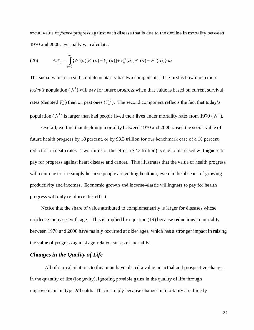
37

social value of future progress against each disease that is due to the decline in mortality between

1970 and 2000. Formally we calculate:

(26) 1 1 0 0 1 0

0

{ ( )[ ( ) ( )] ( )[ ( ) ( )]}a

W N a V a V a V a N a N a daα α α α

∞

=

∆ = − + −∫

The social value of health complementarity has two components. The first is how much more

today’s population ( 1N ) will pay for future progress when that value is based on current survival

rates (denoted 1Vα ) than on past ones ( 0Vα ). The second component reflects the fact that today’s

population ( 1N ) is larger than had people lived their lives under mortality rates from 1970 ( 0N ).

Overall, we find that declining mortality between 1970 and 2000 raised the social value of

future health progress by 18 percent, or by $3.3 trillion for our benchmark case of a 10 percent

reduction in death rates. Two-thirds of this effect ($2.2 trillion) is due to increased willingness to

pay for progress against heart disease and cancer. This illustrates that the value of health progress

will continue to rise simply because people are getting healthier, even in the absence of growing

productivity and incomes. Economic growth and income-elastic willingness to pay for health

progress will only reinforce this effect.

Notice that the share of value attributed to complementarity is larger for diseases whose

incidence increases with age. This is implied by equation (19) because reductions in mortality

between 1970 and 2000 have mainly occurred at older ages, which has a stronger impact in raising

the value of progress against age-related causes of mortality.

Changes in the Quality of Life

All of our calculations to this point have placed a value on actual and prospective changes

in the quantity of life (longevity), ignoring possible gains in the quality of life through

improvements in type-H health. This is simply because changes in mortality are directly

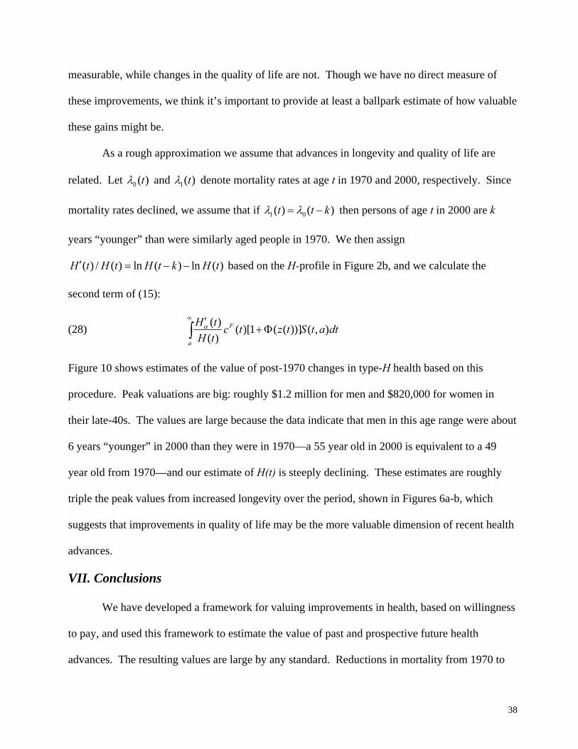
38

measurable, while changes in the quality of life are not. Though we have no direct measure of

these improvements, we think it’s important to provide at least a ballpark estimate of how valuable

these gains might be.

As a rough approximation we assume that advances in longevity and quality of life are

related. Let 0 ( )tλ and 1( )tλ denote mortality rates at age t in 1970 and 2000, respectively. Since

mortality rates declined, we assume that if 1 0( ) ( )t t kλ λ= − then persons of age t in 2000 are k

years “younger” than were similarly aged people in 1970. We then assign

( ) / ( ) ln ( ) ln ( )H t H t H t k H t′ = − − based on the H-profile in Figure 2b, and we calculate the

second term of (15):

(28) ( ) ( )[1 ( ( ))] ( , )( )

F

a

H t c t z t S t a dtH tα

∞ ′+Φ∫

Figure 10 shows estimates of the value of post-1970 changes in type-H health based on this

procedure. Peak valuations are big: roughly $1.2 million for men and $820,000 for women in

their late-40s. The values are large because the data indicate that men in this age range were about

6 years “younger” in 2000 than they were in 1970—a 55 year old in 2000 is equivalent to a 49

year old from 1970—and our estimate of H(t) is steeply declining. These estimates are roughly

triple the peak values from increased longevity over the period, shown in Figures 6a-b, which

suggests that improvements in quality of life may be the more valuable dimension of recent health

advances.

VII. Conclusions

We have developed a framework for valuing improvements in health, based on willingness

to pay, and used this framework to estimate the value of past and prospective future health

advances. The resulting values are large by any standard. Reductions in mortality from 1970 to

39

2000 had an (uncounted) economic value to the 2000 population of the U.S. of about $3.2 trillion

per year. Over the longer term, cumulative longevity gains during the 20th century were worth

about $1.3 million per person to the representative member of the 2000 U.S. population. Valued

at the date they occurred, the production of longevity-related “health capital” would raise

estimates of per-capita output in the U.S. by from 10 to 50 percent, depending on the time period

in question.

Prospectively, even modest progress against mortality causing diseases such as cancer and

heart disease would have enormous social values. A one percent reduction in mortality from

cancer or heart disease would be worth nearly $500 billion to current and future Americans.

These estimates ignore the value of health advances to individuals in other countries, so they

likely understate aggregate social values of possible innovations. They also ignore corresponding

improvements in the quality of life—which evidence suggests may be even more valuable than

gains in longevity—and for these reasons as well they are likely to be conservative. We show that

these values will increase in the future because of economic growth and, more interestingly,

because health itself continues to improve.

Large as they are, these values may be offset by the costs of developing and implementing

improvements in health. Current public and private spending on health-related research is a tiny

fraction of what is on the table, yet such investments may not be worthwhile if the costs of

implementing new technologies is large. Social transfer programs and other third-party methods

of financing health care can distort both utilization decisions and research, with the result that

some health improvements are socially inefficient.

40

References

Arthur, W.B., “The Economics of Risk to Life”, American Economic Review 71, March 1981, 54-

64.

Banks, James; Richard Blundell and Sarah Turner, “Is There a Retirement-Savings Puzzle?”

American Economic Review, vol. 88, No. 4 (Sept., 1998), 769-788

Barsky, Robert, Thomas Juster, Miles Kimball, and Matt Shapiro, “Preference Parameters and

Behavioral Heterogeneity: An Experimental Approach in the Health and Retirement

Survey,” Quarterly Journal of Economics, 12, 1997: 537-580.

Becker, Gary S. and Casey B. Mulligan. “The Endogenous Determination of Time Preference.”

Quarterly Journal of Economics. 112(3), August 1997: 729-58.

Browning, Martin, Lars Peter Hansen, and James J. Heckman “Micro Data and General

Equilibrium Models” in Handbook of Macroeconomics, volume I, ed. John Taylor and

Michael Woodford, Elsevier Science, 1999.

Browning, Martin, and Thomas Crossley, “The Life-Cycle Model of Consumption and Saving”,

Journal of Economic Perspectives, Vol. 15, No. 3 (Summer, 2001), 3-22.

Campbell, John and Gregory Mankiw, “Consumption, Income, and Interest Rates: Reinterpreting

the Time Series Evidence” NBER Macroeconomics Annual 4, 1989: 185-216

Cutler, David. “Technology, Health Costs, and the NIH,” Unpublished paper prepared for NIH

Roundtable on Economics, October 19, 1995.

Cutler, David, and Richardson, Elizabeth. “Measuring the Health of the U.S. Population,”

Brookings Papers: Microeconomics 1997, pp. 217-271.

Dockins, Chris, Kelly Maguire, Nathalie Simon and Melonie Sullivan, “Value of Statistical Life

Analysis and Environmental Policy: A White Paper”, U.S. Environmental Protection

Agency, National Center for Environmental Economics, April 2004.

V.R. Fuchs, “Health Care and the United States Economic System: An Essay in Abnormal

Physiology,” Milbank Quarterly 50, no. 2 (1972): 211–237.

Hogan, Christopher, June Lunney, Jon Gabel, and Lynn, "Medicare beneficiaries' costs of care in

the last year of life," Health Affairs 20(4), July 2001,pp. 188-195.

Griliches, Zvi, and Lichtenberg, Frank. “R&D and Productivity at the Industry Level: Is There

Still a Relationship?” in R&D, Patents, and Productivity, edited by Zvi Griliches.

Chicago: University of Chicago Press, 1984.

41

Hall, Robert “Intertemporal Substitution in Consumption”, Journal of Political Economy, 96(2),

1988: 339-357.

Hansen, Lars Peter and Kenneth Singleton “Stochastic Consumption, Risk Aversion, and the

Temporal Behavior of Asset Returns, Journal of Political Economy, 91(2), 1983, 249-265.

Jones, Matthew T. and Maurice Obstfeld, “Saving, Investment, and Gold: A Reassessment of

Historical Current Account Data,” from Money, Capital Mobility, and Trade: Essays in

Honor of Robert Mundell, ed. Guillermo Calvo, Rudiger Dornbusch and Maurice Obstfeld,

(Cambridge, MA, MIT Press, 2001)

Lichtenberg, Frank R. “The Allocation of Publicly-Funded Biomedical Research,” National

Bureau of Economic Research Working Paper No. 6601. Cambridge, MA: NBER, June

1998.

Meltzer, David, “Can Medical Cost Effectiveness Analysis Identify the Value of Medical

Research?”, in Measuring the Gains from Medical Research: An Economic Approach,

edited by Kevin M. Murphy and Robert H. Topel. Chicago: University of Chicago Press,

2003.

Murphy, Kevin M. and Robert H. Topel (2003a),“The Economic Value of Medical Research” , in

Measuring the Gains from Medical Research: An Economic Approach, edited by Kevin M.

Murphy and Robert H. Topel. Chicago: University of Chicago Press, 2003.

Murphy, Kevin M. and Robert H. Topel (2003b), “Diminishing Returns? Evidence on the Costs

and Benefits of Improving Health”, Perspectives in Biology and Medicine, volume 46, no.

3, (Summer, 2003): pp108-128.

Murphy, Kevin and Robert H. Topel, “Black-White Differences in the Economic Value of

Improving Health”, Perspectives in Biology and Medicine, vol 47, no. 3, (Summer, 2004).

Nordhaus, William D. "The Health of Nations: The Contribution of Improved Health to Living

Standards." in Measuring the Gains from Medical Research: An Economic Approach,

edited by Kevin M. Murphy and Robert H. Topel. Chicago: University of Chicago Press,

2003.

Rosen, Sherwin. “The Quantity and Quality of Life: A Conceptual Framework”, in George Tolley,

Donald Kenkel, and Robert Fabian, Valuing Health for Policy, University of Chicago

Press, 1994.

42

Thaler, Richard and Sherwin Rosen “The Value of Saving a Life: Evidence from the Labor

Market. In Household Production and Consumption, ed. Nestor E. Terleckyj, New York,

NBER, 1975.

Tolley, George, Donald Kenkel and Robert Fabian “State of the Art Health Values” in Tolley et.

al. Valuing Health for Policy, University of Chicago Press for NBER, 1994.

Topel, Robert H., and Finis Welch. “Efficient Labor Contracts with Employment Risk,” Rand

Journal of Economics 17 (Winter 1986): 490-507.

United States Environmental Protection Agency, Science Advisory Board, “SAB Report from the

Environmental Economics Advisory Committee on EPA’s White Paper ‘Valuing the

Benefits of Fatal Cancer Risk Reduction”, July 27, 2000.

Viscusi, W. Kip. “The Value of Risks to Life and Health,” Journal of Economic Literature 31

(1993): 1912-1946.

Viscusi, W. Kip and Joseph E. Aldy, “The Value of a Statistical Life: A Critical Review of Market

Estimates Throughout the World”, Brookings Joint Center for Regulatory Studies, January

2003.

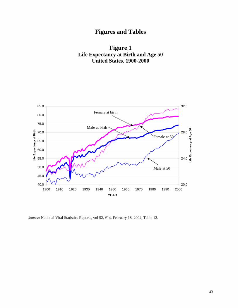
43

Figures and Tables

Figure 1 Life Expectancy at Birth and Age 50

United States, 1900-2000

40.0

45.0

50.0

55.0

60.0

65.0

70.0

75.0

80.0

85.0

1900 1910 1920 1930 1940 1950 1960 1970 1980 1990 2000

YEAR

Life

Exp

ecta

ncy

at B

irth

20.0

24.0

28.0

32.0

Life

Exp

ecta

ncy

at A

ge 5

0

Source: National Vital Statistics Reports, vol 52, #14, February 18, 2004, Table 12.

Female at birth

Female at 50

Male at birth

Male at 50

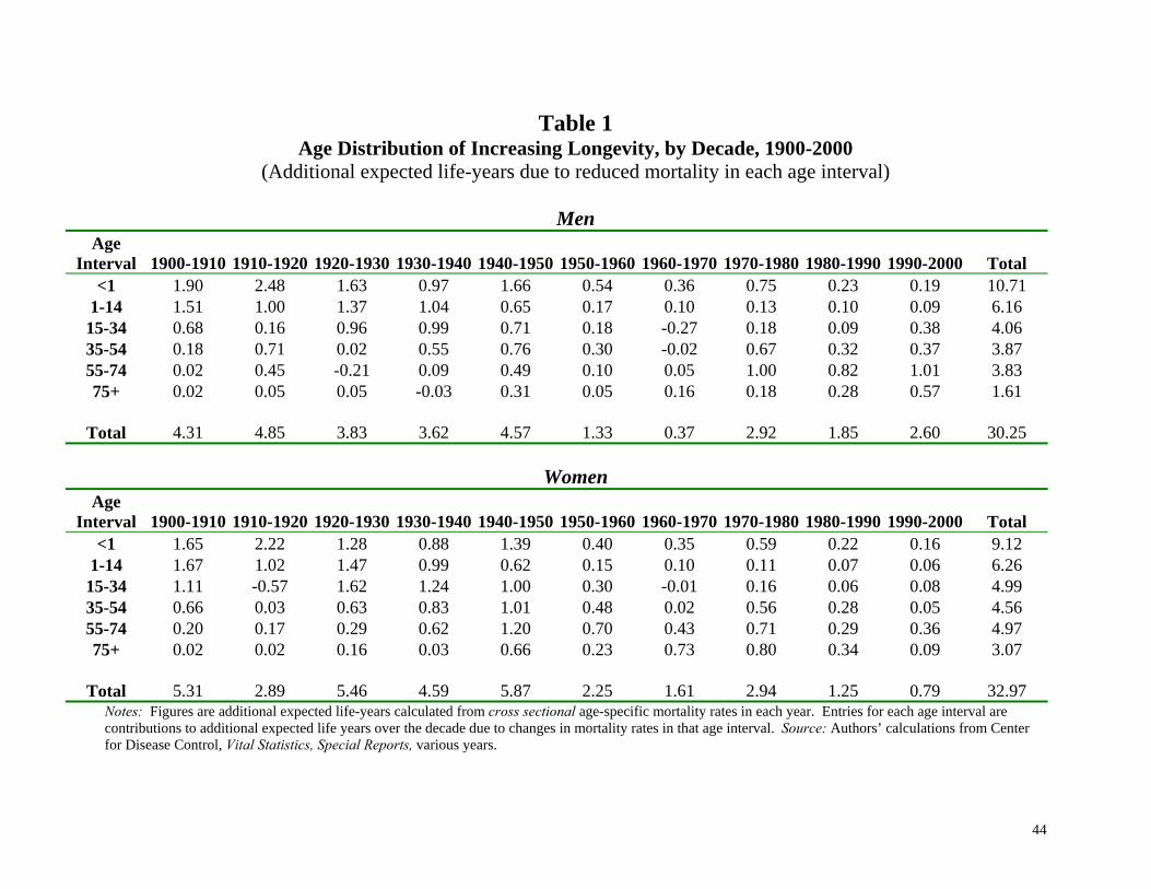
44

Table 1 Age Distribution of Increasing Longevity, by Decade, 1900-2000

(Additional expected life-years due to reduced mortality in each age interval)

Men

Age Interval 1900-1910 1910-1920 1920-1930 1930-1940 1940-1950 1950-1960 1960-1970 1970-1980 1980-1990 1990-2000

Total

<1 1.90 2.48 1.63 0.97 1.66 0.54 0.36 0.75 0.23 0.19 10.71 1-14 1.51 1.00 1.37 1.04 0.65 0.17 0.10 0.13 0.10 0.09 6.16 15-34 0.68 0.16 0.96 0.99 0.71 0.18 -0.27 0.18 0.09 0.38 4.06 35-54 0.18 0.71 0.02 0.55 0.76 0.30 -0.02 0.67 0.32 0.37 3.87 55-74 0.02 0.45 -0.21 0.09 0.49 0.10 0.05 1.00 0.82 1.01 3.83 75+ 0.02 0.05 0.05 -0.03 0.31 0.05 0.16 0.18 0.28 0.57 1.61

Total 4.31 4.85 3.83 3.62 4.57 1.33 0.37 2.92 1.85 2.60 30.25

Women

Age Interval 1900-1910 1910-1920 1920-1930 1930-1940 1940-1950 1950-1960 1960-1970 1970-1980 1980-1990 1990-2000

Total

<1 1.65 2.22 1.28 0.88 1.39 0.40 0.35 0.59 0.22 0.16 9.12 1-14 1.67 1.02 1.47 0.99 0.62 0.15 0.10 0.11 0.07 0.06 6.26 15-34 1.11 -0.57 1.62 1.24 1.00 0.30 -0.01 0.16 0.06 0.08 4.99 35-54 0.66 0.03 0.63 0.83 1.01 0.48 0.02 0.56 0.28 0.05 4.56 55-74 0.20 0.17 0.29 0.62 1.20 0.70 0.43 0.71 0.29 0.36 4.97 75+ 0.02 0.02 0.16 0.03 0.66 0.23 0.73 0.80 0.34 0.09 3.07

Total 5.31 2.89 5.46 4.59 5.87 2.25 1.61 2.94 1.25 0.79 32.97

Notes: Figures are additional expected life-years calculated from cross sectional age-specific mortality rates in each year. Entries for each age interval are contributions to additional expected life years over the decade due to changes in mortality rates in that age interval. Source: Authors’ calculations from Center for Disease Control, Vital Statistics, Special Reports, various years.

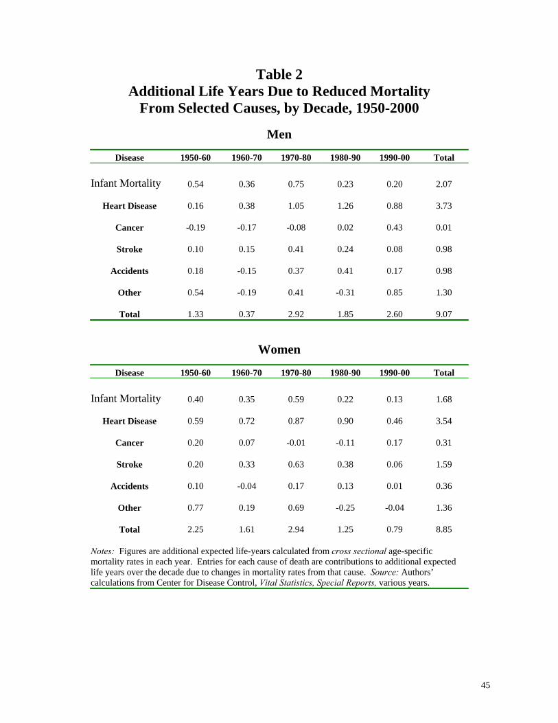
45

Table 2 Additional Life Years Due to Reduced Mortality

From Selected Causes, by Decade, 1950-2000

Men

Women

Disease 1950-60 1960-70 1970-80 1980-90 1990-00 Total Infant Mortality 0.54 0.36 0.75 0.23 0.20 2.07

Heart Disease 0.16 0.38 1.05 1.26 0.88 3.73

Cancer -0.19 -0.17 -0.08 0.02 0.43 0.01

Stroke 0.10 0.15 0.41 0.24 0.08 0.98

Accidents 0.18 -0.15 0.37 0.41 0.17 0.98

Other 0.54 -0.19 0.41 -0.31 0.85 1.30

Total 1.33 0.37 2.92 1.85 2.60 9.07

Disease 1950-60 1960-70 1970-80 1980-90 1990-00 Total Infant Mortality 0.40 0.35 0.59 0.22 0.13 1.68

Heart Disease 0.59 0.72 0.87 0.90 0.46 3.54

Cancer 0.20 0.07 -0.01 -0.11 0.17 0.31

Stroke 0.20 0.33 0.63 0.38 0.06 1.59

Accidents 0.10 -0.04 0.17 0.13 0.01 0.36

Other 0.77 0.19 0.69 -0.25 -0.04 1.36

Total 2.25 1.61 2.94 1.25 0.79 8.85

Notes: Figures are additional expected life-years calculated from cross sectional age-specific mortality rates in each year. Entries for each cause of death are contributions to additional expected life years over the decade due to changes in mortality rates from that cause. Source: Authors’ calculations from Center for Disease Control, Vital Statistics, Special Reports, various years.

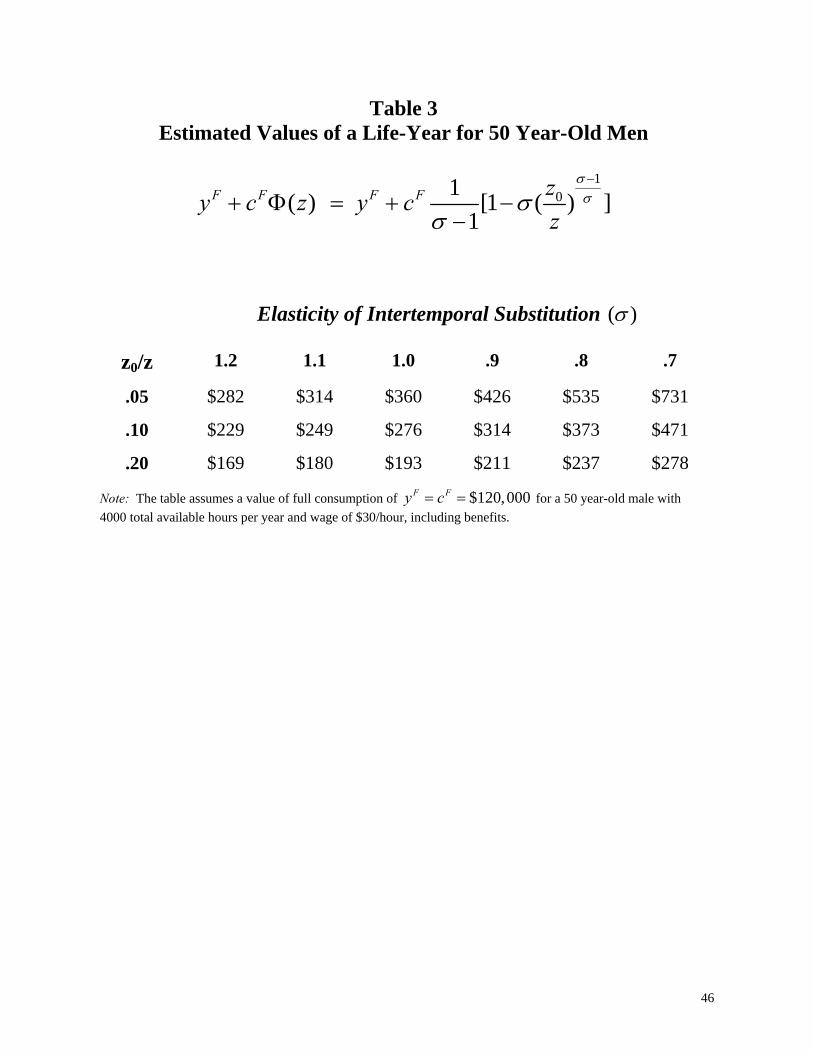
46

Table 3 Estimated Values of a Life-Year for 50 Year-Old Men

1

01( ) [1 ( ) ]1

F F F F zy c z y cz

σσσ

σ

−

+ Φ = + −−

Elasticity of Intertemporal Substitution ( )σ

z0/z

1.2

1.1

1.0

.9

.8

.7

.05

$282

$314

$360

$426

$535

$731

.10

$229

$249

$276

$314

$373

$471

.20

$169

$180

$193

$211

$237

$278

Note: The table assumes a value of full consumption of $120,000F Fy c= = for a 50 year-old male with 4000 total available hours per year and wage of $30/hour, including benefits.

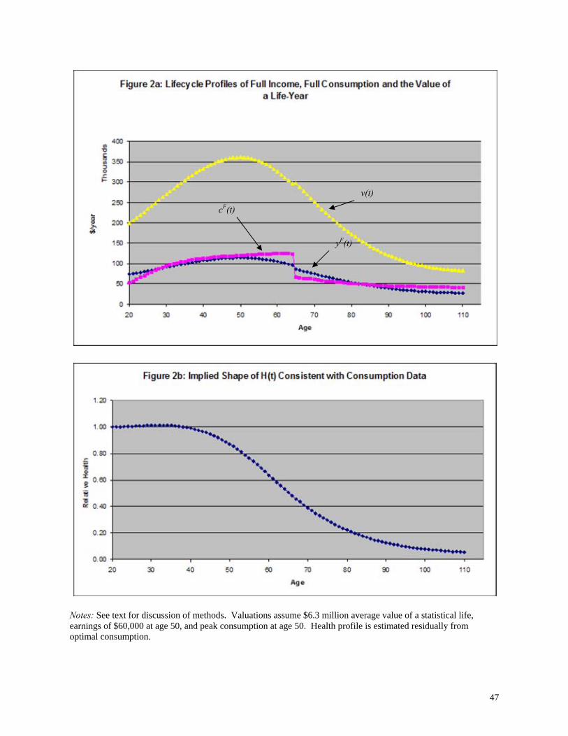
47

Notes: See text for discussion of methods. Valuations assume $6.3 million average value of a statistical life, earnings of $60,000 at age 50, and peak consumption at age 50. Health profile is estimated residually from optimal consumption.

v(t)

cF(t)

yF(t)

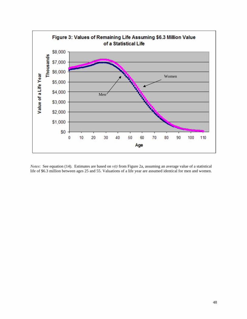
48

Notes: See equation (14). Estimates are based on v(t) from Figure 2a, assuming an average value of a statistical life of $6.3 million between ages 25 and 55. Valuations of a life year are assumed identical for men and women.

Women

Men

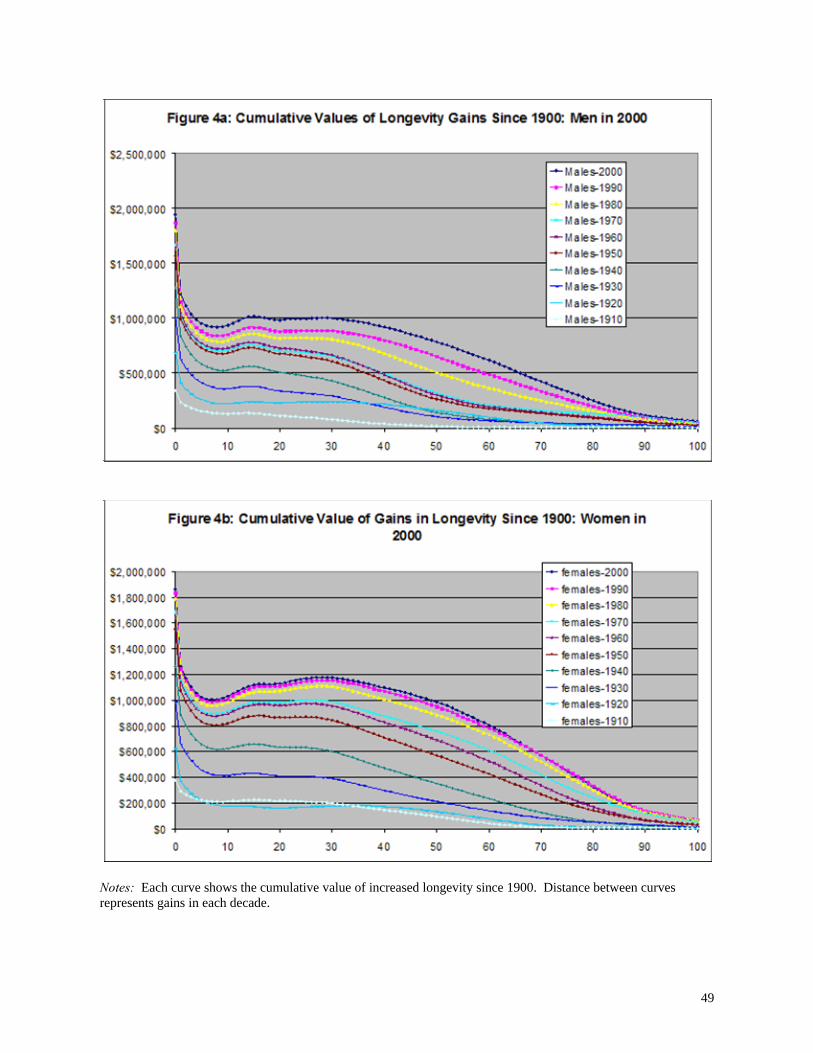
49

Notes: Each curve shows the cumulative value of increased longevity since 1900. Distance between curves represents gains in each decade.

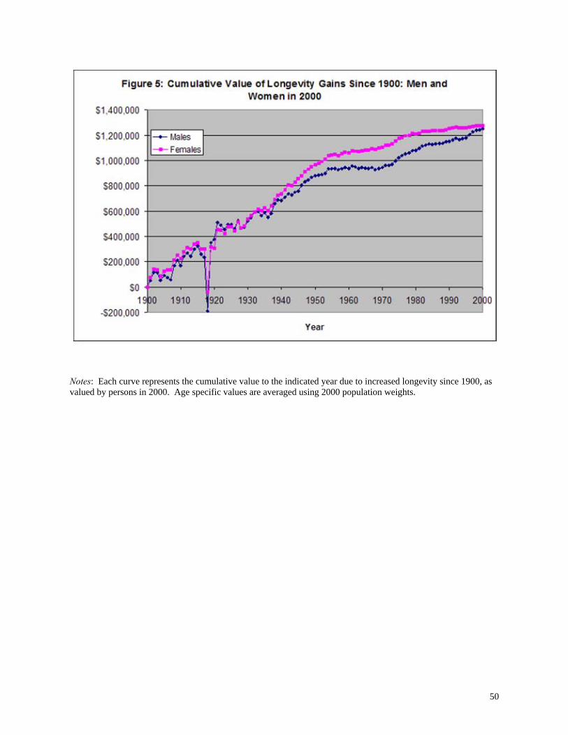
50

Notes: Each curve represents the cumulative value to the indicated year due to increased longevity since 1900, as valued by persons in 2000. Age specific values are averaged using 2000 population weights.

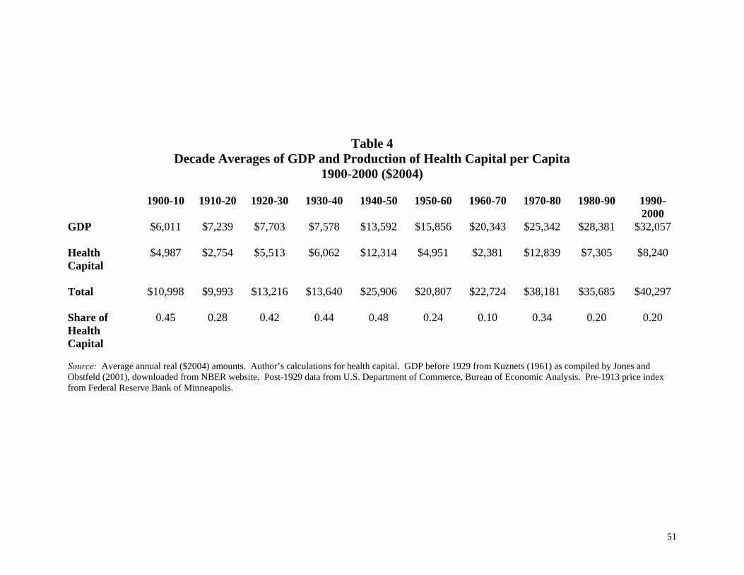
51

Table 4 Decade Averages of GDP and Production of Health Capital per Capita

1900-2000 ($2004)

1900-10 1910-20 1920-30 1930-40 1940-50 1950-60 1960-70 1970-80 1980-90 1990-2000

GDP $6,011 $7,239 $7,703 $7,578 $13,592 $15,856 $20,343 $25,342 $28,381 $32,057 Health Capital

$4,987 $2,754 $5,513 $6,062 $12,314 $4,951 $2,381 $12,839 $7,305 $8,240

Total $10,998 $9,993 $13,216 $13,640 $25,906 $20,807 $22,724 $38,181 $35,685 $40,297 Share of Health Capital

0.45 0.28 0.42 0.44 0.48 0.24 0.10 0.34 0.20 0.20

Source: Average annual real ($2004) amounts. Author’s calculations for health capital. GDP before 1929 from Kuznets (1961) as compiled by Jones and Obstfeld (2001), downloaded from NBER website. Post-1929 data from U.S. Department of Commerce, Bureau of Economic Analysis. Pre-1913 price index from Federal Reserve Bank of Minneapolis.

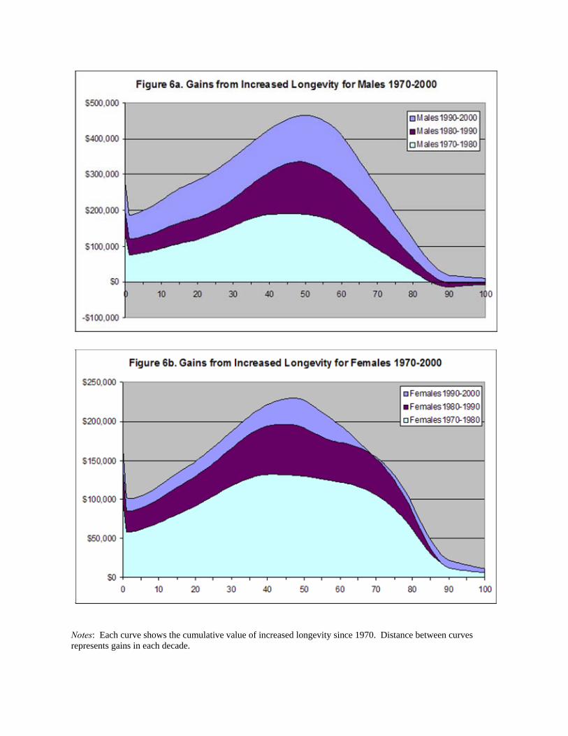
Notes: Each curve shows the cumulative value of increased longevity since 1970. Distance between curves represents gains in each decade.

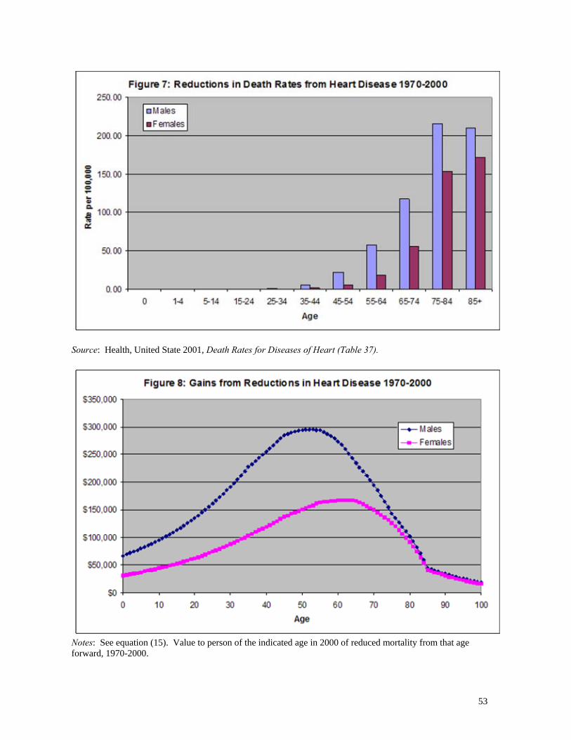
53

Source: Health, United State 2001, Death Rates for Diseases of Heart (Table 37).

Notes: See equation (15). Value to person of the indicated age in 2000 of reduced mortality from that age forward, 1970-2000.

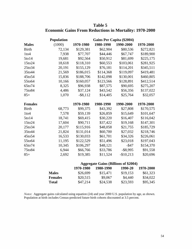
54

Table 5 Economic Gains From Reductions in Mortality: 1970-2000

Population Gains Per Capita ($2004) Males (1000) 1970-1980 1980-1990 1990-2000 1970-2000 Birth 72,134 $129,381 $62,904 $80,536 $272,8211to4 7,938 $77,707 $44,446 $67,747 $189,9005to14 19,681 $92,564 $50,912 $81,699 $225,17515to24 18,618 $118,310 $60,553 $103,061 $281,92525to34 20,191 $155,129 $76,181 $114,201 $345,51135to44 21,569 $186,015 $114,368 $119,097 $419,48145to54 15,836 $188,706 $142,098 $130,001 $460,80555to64 10,166 $160,057 $123,566 $128,891 $412,51465to74 8,325 $96,938 $87,575 $90,695 $275,20775to84 4,486 $37,124 $43,542 $56,356 $137,02285+ 1,070 -$8,112 $14,405 $25,764 $32,057

Females 1970-1980 1980-1990 1990-2000 1970-2000 Birth 68,773 $99,375 $43,392 $27,808 $170,5751to4 7,578 $59,139 $26,859 $15,649 $101,6475to14 18,741 $69,415 $30,220 $16,407 $116,04215to24 17,604 $90,711 $37,422 $19,168 $147,30125to34 20,177 $115,916 $48,058 $21,755 $185,72935to44 21,824 $131,014 $60,700 $27,032 $218,74645to54 16,533 $130,033 $61,701 $34,326 $226,06155to64 11,195 $122,529 $51,496 $23,018 $197,04365to74 10,345 $106,297 $48,121 -$47 $154,37075to84 6,944 $66,766 $33,786 -$8,995 $91,55885+ 2,692 $19,385 $11,524 -$10,213 $20,696

Aggregate Gains (Billions of $2004) 1970-1980 1980-1990 1990-20 1970-2000 Males $26,699 $15,471 $19,153 $61,323 Females $20,515 $9,067 $4,440 $34,022 Total $47,214 $24,538 $23,593 $95,345

Notes: Aggregate gains calculated using equation (24) and year 2000 U.S. population by age, as shown. Population at birth includes Census-predicted future birth cohorts discounted at 3.5 percent.

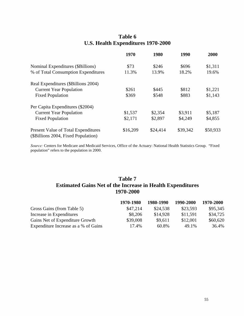
55

Table 6

U.S. Health Expenditures 1970-2000 1970 1980 1990 2000

Nominal Expenditures ($Billions) $73 $246 $696 $1,311 % of Total Consumption Expenditures 11.3% 13.9% 18.2% 19.6%

Real Expenditures ($Billions 2004) Current Year Population $261 $445 $812 $1,221 Fixed Population $369 $548 $883 $1,143

Per Capita Expenditures ($2004) Current Year Population $1,537 $2,354 $3,911 $5,187 Fixed Population $2,171 $2,897 $4,249 $4,855

Present Value of Total Expenditures $16,209 $24,414 $39,342 $50,933 ($Billions 2004, Fixed Population)

Source: Centers for Medicare and Medicaid Services, Office of the Actuary: National Health Statistics Group. “Fixed population” refers to the population in 2000.

Table 7 Estimated Gains Net of the Increase in Health Expenditures

1970-2000 1970-1980 1980-1990 1990-2000 1970-2000

Gross Gains (from Table 5) $47,214 $24,538 $23,593 $95,345Increase in Expenditures $8,206 $14,928 $11,591 $34,725Gains Net of Expenditure Growth $39,008 $9,611 $12,001 $60,620Expenditure Increase as a % of Gains 17.4% 60.8% 49.1% 36.4%

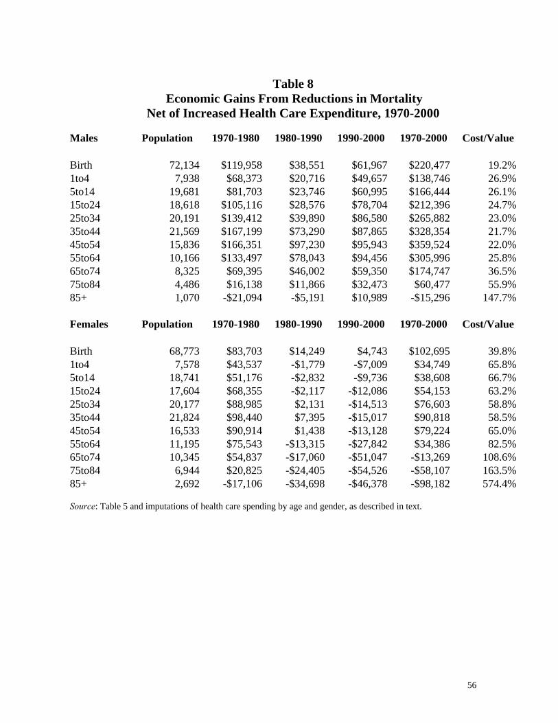
56

Table 8

Economic Gains From Reductions in Mortality Net of Increased Health Care Expenditure, 1970-2000

Males Population 1970-1980 1980-1990 1990-2000 1970-2000 Cost/Value

Birth 72,134 $119,958 $38,551 $61,967 $220,477 19.2%1to4 7,938 $68,373 $20,716 $49,657 $138,746 26.9%5to14 19,681 $81,703 $23,746 $60,995 $166,444 26.1%15to24 18,618 $105,116 $28,576 $78,704 $212,396 24.7%25to34 20,191 $139,412 $39,890 $86,580 $265,882 23.0%35to44 21,569 $167,199 $73,290 $87,865 $328,354 21.7%45to54 15,836 $166,351 $97,230 $95,943 $359,524 22.0%55to64 10,166 $133,497 $78,043 $94,456 $305,996 25.8%65to74 8,325 $69,395 $46,002 $59,350 $174,747 36.5%75to84 4,486 $16,138 $11,866 $32,473 $60,477 55.9%85+ 1,070 -$21,094 -$5,191 $10,989 -$15,296 147.7%

Females Population 1970-1980 1980-1990 1990-2000 1970-2000 Cost/Value

Birth 68,773 $83,703 $14,249 $4,743 $102,695 39.8%1to4 7,578 $43,537 -$1,779 -$7,009 $34,749 65.8%5to14 18,741 $51,176 -$2,832 -$9,736 $38,608 66.7%15to24 17,604 $68,355 -$2,117 -$12,086 $54,153 63.2%25to34 20,177 $88,985 $2,131 -$14,513 $76,603 58.8%35to44 21,824 $98,440 $7,395 -$15,017 $90,818 58.5%45to54 16,533 $90,914 $1,438 -$13,128 $79,224 65.0%55to64 11,195 $75,543 -$13,315 -$27,842 $34,386 82.5%65to74 10,345 $54,837 -$17,060 -$51,047 -$13,269 108.6%75to84 6,944 $20,825 -$24,405 -$54,526 -$58,107 163.5%85+ 2,692 -$17,106 -$34,698 -$46,378 -$98,182 574.4% Source: Table 5 and imputations of health care spending by age and gender, as described in text.

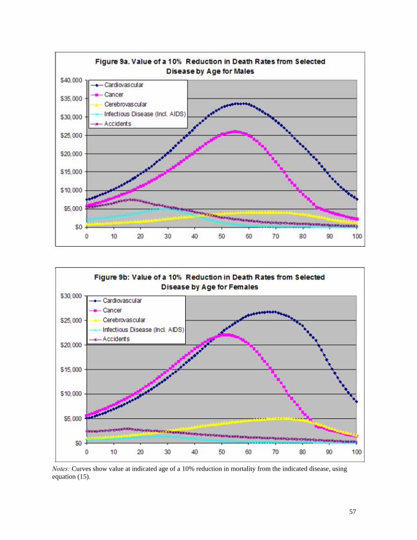
57

Notes: Curves show value at indicated age of a 10% reduction in mortality from the indicated disease, using equation (15).

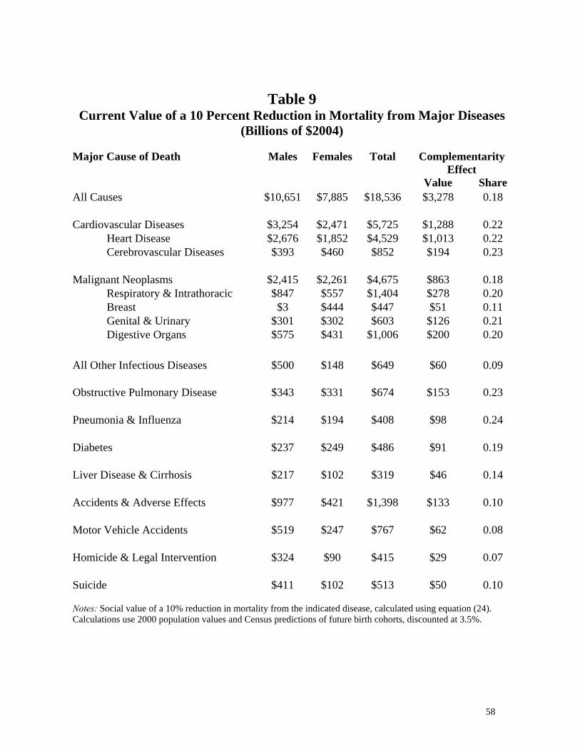
58

Table 9 Current Value of a 10 Percent Reduction in Mortality from Major Diseases

(Billions of $2004)

Major Cause of Death Males Females Total Complementarity Effect

Value Share All Causes $10,651 $7,885 $18,536 $3,278 0.18

Cardiovascular Diseases $3,254 $2,471 $5,725 $1,288 0.22

Heart Disease $2,676 $1,852 $4,529 $1,013 0.22 Cerebrovascular Diseases $393 $460 $852 $194 0.23

Malignant Neoplasms $2,415 $2,261 $4,675 $863 0.18

Respiratory & Intrathoracic $847 $557 $1,404 $278 0.20 Breast $3 $444 $447 $51 0.11 Genital & Urinary $301 $302 $603 $126 0.21 Digestive Organs $575 $431 $1,006 $200 0.20

All Other Infectious Diseases $500 $148 $649 $60 0.09

Obstructive Pulmonary Disease $343 $331 $674 $153 0.23

Pneumonia & Influenza $214 $194 $408 $98 0.24

Diabetes $237 $249 $486 $91 0.19

Liver Disease & Cirrhosis $217 $102 $319 $46 0.14

Accidents & Adverse Effects $977 $421 $1,398 $133 0.10

Motor Vehicle Accidents $519 $247 $767 $62 0.08

Homicide & Legal Intervention $324 $90 $415 $29 0.07

Suicide $411 $102 $513 $50 0.10 Notes: Social value of a 10% reduction in mortality from the indicated disease, calculated using equation (24). Calculations use 2000 population values and Census predictions of future birth cohorts, discounted at 3.5%.

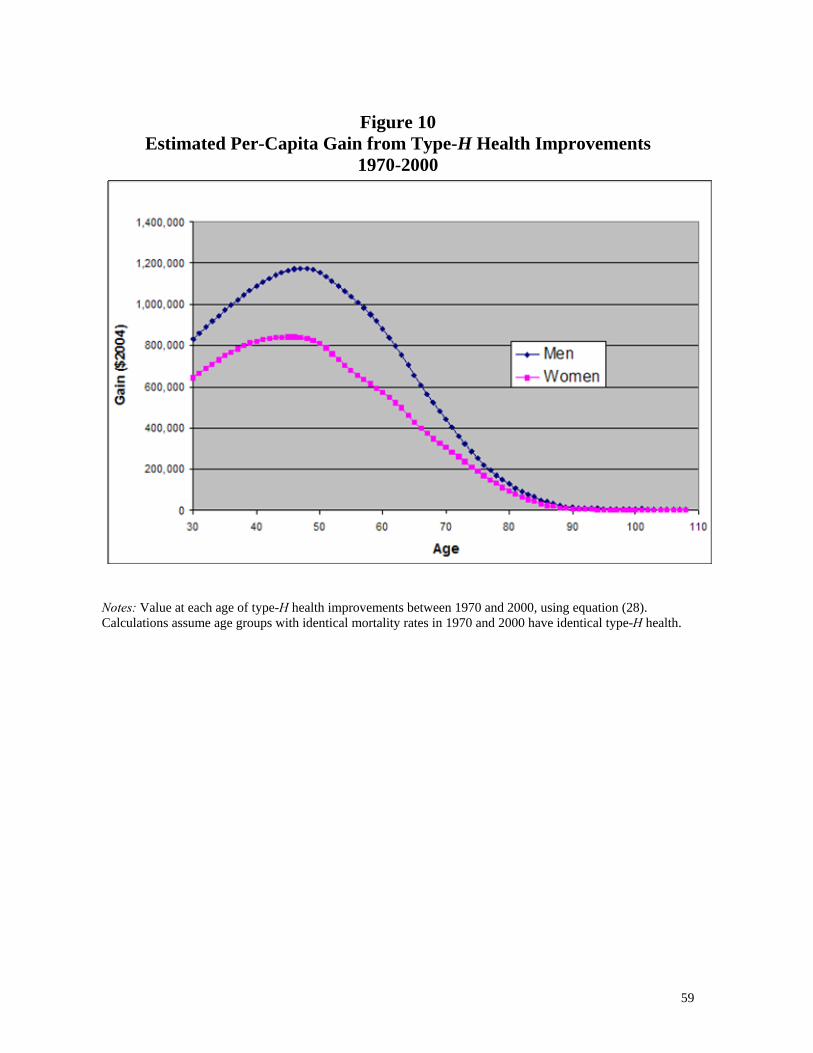
59

Figure 10

Estimated Per-Capita Gain from Type-H Health Improvements 1970-2000

Notes: Value at each age of type-H health improvements between 1970 and 2000, using equation (28). Calculations assume age groups with identical mortality rates in 1970 and 2000 have identical type-H health.