THE VALUATION OF FOREIGN CURRENCY OPTIONS IN KENYA

UNDER STOCHASTIC VOLATILITY

BY: KAMBI ROBINSONMUNENE D61/63201/2011

A Management Research Project Submitted In Partial Fulfillment of theRequirements for the Degree of Masters of Business Administration (MBA),

School Of Business, University Of Nairobi

NOVEMBER 2013

DECLARATIO

N

This research project is my original work and has not been submitted for the award of a degree at anyother university.

Signed…………………………………………………… Date………………………………….

Kambi Robinson Munene. Registration

Number: D61/63201/2011.

This research project has been submitted for examination with my approval as a University of Nairobi supervisor.

Signed…………………………………………………….Date………………………………….

Dr. Aduda Josiah O. Senior Lecturer. School of Business, University of Nairobi.

DEDICATIO

N

I dedicate this research project to my loving family; my mother and three sisters all of whom havebeen a source of great inspiration in all my endevours.May the Almighty God bless them abundantly.

ACKNOWLEDGEMENT

S

I would first like to acknowledge my supervisor Dr.Josiah O Aduda whose guidance, input and insight

has enabled me complete the research project. I am particularly grateful for his patience, insightful

comments and advice throughout the entire process the project. I would also like to acknowledge my

moderatorMr.MwangiMirie for the helpful and insightful input and comments all of which were very

important in conducting this research project.

I would also like to acknowledge the contribution made by Mr.Tirop of Central Bank of Kenya in this

project, I especially acknowledge him for the adequate and helpful assistance that he gave me in the

certification of the secondary data that I used.

Lastly I would like to acknowledge the University Of Nairobi Masters Of Business Administration(MBA) for the assistance they gave me throughout the whole process of coming up with this projectand without forgetting MBA students University of Nairobi for the constructive criticism and insight.May God bless you all.

ABSTRAC

T

The main objective of this research project is to show how foreign currency options can be valued in

Kenya under stochastic volatility and also to come up with a model for predicting variance and

volatility of exchange rates. First the research sought to develop a model for predicting variance based

on the USD and Kenya Shillings exchange rates in Kenya for a period of five years between 2008-

2012.The research also sought to show how foreign currency options would be priced information

from the available data.

This research used descriptive research design and the Garman Kohlhagen model for valuation of

foreign currency options. The research uses Garch (1, 1) model to fit the variance regression line

which was used to predict variance and subsequently the volatility that together with other variables

isplugged into the Garman Kohlhagen model. to price the foreign currency options.

The research gave findings that were consistent with research done in the area of valuation of foreigncurrency options. The research shown that foreign currency options can be valued in Kenya by use ofa Garch (1, 1) framework which was a good fit for the actual data as the coefficients of the modelwere within the model constraints of (+ 0.98) <1 for using Garch (1, 1) .The research found out thatfor call options when the spot exchange rate is below the strike price the option has statistically zerovalue and when above strike price the option has a positive value. On the other hand the price of a putcurrency option is positive when the spot exchange rate is below the strike price and statistically zerowhen the spot exchange rates are above the strike prices and the further away from the strike price thespot exchange rate is the higher the value of the option.

ABBREVIATION

S

ATM……………….. At-the-money ARCH……………….Auto Regressive Conditional Heteroscedasticity BA-W……………….. Barone Adesi Whaley Model.B-S…………………..Black Scholes Model. CMA………………...Capital Markets Authority. GARCH…………….Generalized Autoregressive Conditional Heteroscedasticity GBP………………….Great Britain Pound ITM…………….. …..In-the-money JPY…………………..Japanese Yen. NSE…………………Nairobi Securities Exchange. OTC…………………Over the Counter. OTM………………… Out-the-money PHLX ……………….Philadelphia Stock Exchange REITS………………Real Estate Investments Trusts. USD…………………United States Dollar.

TABLE

S

Table 1……………………………………Model Summary.

Table 2……………………………………Coefficients. Table

3………………………………….. Strike price at 70. Table

4…………………………………… Strike price at 80. Table

5…………………………………… Strike price at 90. Table

6…………………………………… Strike price at 100.

TABLE OF CONTENT

S

DECLARATION .............................................................................................................

................. i

DEDICATION.................................................................................................................

.................ii ACKNOWLEDGEMENTS

.............................................................................................................iii

ABSTRACT....................................................................................................................

.................iv

ABBREVIATIONS...........................................................................................................

................v TABLES

.....................................................................................................................................

.....vi CHAPTER

ONE..............................................................................................................................

.1 INTRODUCTION

............................................................................................................................1

1.1. Background of the Study....................................................................................................1

1.1.1. Capital Market in Kenya and Foreign Currency Options...........................................3

1.2. Statement of the Problem...................................................................................................5

1.3. ResearchObjectives...........................................................................................................7

1.4 Significance of the Study ....................................................................................................7

CHAPTERTWO.............................................................................................................................

.9 LITERATURE REVIEW.................................................................................................................9 2.1

Introduction.......................................................................................................................9 2.2 Review of

Theories...........................................................................................................10 2.2.1 Black-Scholes Model.................................................................................................10

2.2.2 Garman and Kohlhagen model.................................................................................12

2.2.3 Binomial option pricing model..................................................................................13

2.3 Review of Empirical Studies.............................................................................................15

2.4 Conclusion from literature review....................................................................................21

CHAPTERTHREE........................................................................................................................2

3 RESEARCHMETHODOLOGY....................................................................................................23 3.1

Introduction.....................................................................................................................23 3.2 Research design

...............................................................................................................23 3.3

Population........................................................................................................................23 3.4 Sample

.............................................................................................................................24 3.5 Data Collection

................................................................................................................24 3.6 Data Analysis

...................................................................................................................24 3.7 Conceptual model

............................................................................................................25

3.8 Empirical model

...............................................................................................................2

5

3.9 Data Validity & Reliability....................................................................................................27 CHAPTER FOUR

..........................................................................................................................28DATA ANALYSIS AND PRESENTATION

...............................................................................28 4.1 Introduction.................................................................................................................28 4.2 Data Presentation.........................................................................................................28 4.2.1 Variance...................................................................................................................28 4.2.2 Squared log Returns .................................................................................................28

4.2.3 Risk free rate............................................................................................................29 4.2.4 Strike price...............................................................................................................29 4.2.5 Time to maturity.......................................................................................................30

4.2.6 Volatility...................................................................................................................30 4.3 Regression results analysis and application of model....................................................31

4.4 Summary and Interpretation ofFindings............................................................................37 CHAPTER

FIVE............................................................................................................................39 SUMMARY, CONCLUSIONS AND RECOMMENDATIONS

..................................................39 5.1 Summary......................................................................................................................39 5.2 Conclusions..................................................................................................................40 5.3 Policy Recommendations..............................................................................................41

5.4 Limitations of the Study ...............................................................................................42

5.5 Suggestions for FurtherStudies....................................................................................43REFERENCES...............................................................................................................................44 APPENDICES................................................................................................................................49

CHAPTER ON

E

INTRODUCTION

1.1. Background of the Study

Currency options are derivative financial instrument where there is an agreement between two parties

that gives the purchaser the right, but not the obligation, to exchange a given amount of one currency

for another, at a specified rate, on an agreed date in the future. Currency options insure the purchaser

against adverse exchange rate movements. According to Mixon (2011) foreign exchange option

markets were active during and after the First World War where call options on German marks were

the dominant instrument, but calls on French francs, Italian lira, and other currencies also traded. The

largest clientele for the options consisted of optimistic investors of German heritage. Initially there

were fixed exchange rate regimes in operation and hence this limited growth of the foreign currency

options market.

Trading in foreign currency options began in 1970’s and 1980’s in listed futures and options market ofChicago, Philadelphia and London but from 1990’s the trading in foreign currency options shifted tothe over the counter market.While options on foreign currencies are traded on several organizedexchanges, liquidity in currency options trading is predominant in (OTC) market. Liquidity incurrency options trading is centered in (OTC) market. In fact, according to Malz (1998), the prices ofOTC currency options provide a better expression of changing views of future exchange rates than doprices of exchange traded currency options. According to Chance (2008) the currency options aretherefore a useful tool for a business to use in order to reduce costs and increase benefits from havingincreasing certainty in financial transactions that involve currency conversions.

In pricing of foreign currency options there are various terms as defined in Welch (2009) :First a derivative financial instrument as a financial instrument that derives its value from an underlying asset which in foreign currency options is the exchange rate, there are two types of foreign currency options a call currency option and a put currency option. A call optionon a particular currency gives the holder the right but not an obligation to buy that currency at a predetermined exchange rate at a particular date and a foreign currency put option gives the holder the right to sell the currency at a predetermined exchange rate at a particular date. The seller or writer of the option, receives a payment, referred to as the optionpremium, that then obligates him to sell the exchange currency at the pre specified price known as the strike price,if the option purchaser chooses to exercise his right tobuy or sell the currency. The holder will only decide to exchange currencies if the strike price is a more favorable rate than can be obtained in the spot market at expiration.

Foreign currency options can either be European style that can only be exercised on the expiry date orAmerican style that can be exercised at any day and up to the expiry date .Foreign currency options can either be traded in exchange markets which occur in developed financial markets that have an option market or be traded over the counter. Over the counter traded foreign currency options are better for they can be customized further to offer more flexibility. The majority of currency options traded over the counter (OTC) are European style. The date on which the foreign currency option contract ends is called the expiration date. Currency options can be at the money (ATM) where currency options have an exercise price equal to the spot rate of the underlying currency, in the money(ITM) where currency options may be profitable,

excluding premium costs, if exercised immediately or the foreign currency options may be Out the money (OTM) options would not be profitable, excluding the premium costs, if exercised.

According to Kotz’e (2011) the holder of a call option on a currency will only exercise the option if

the underlying currency is trading in the market at a higher price than the strike price of the option.

The call option gives the right to buy, so in exercising it the holder buys currency at the strike price

and can then sell it in the market at a higher price. Similarly, the holder of a put option on a currency

will only exercise the option if the spot currency is trading in the market at a lower price than the

strike price. The put option gives the right to sell, so in exercising it the holder sells currency at the

strike price and can then buy it in the market at a lower price. From the point of view of the option

holder, the negative profit and loss represent the premium that is paid for the option. Thus, the

premium is the maximum loss that can result from purchasing an option.

1.1.1. Capital Market in Kenya and Foreign Currency Options

According to Aloo (2011) in the emerging markets capital account liberalization has increased currency exposures of both domestic and foreign entities. The demand for instruments to manage the currency risk associated with portfolio investment, as well as foreign direct investment, is expanding quickly. In Kenya the capital account has been liberalized hence leading to increased currency risk exposure hence the need to develop an appropriate foreign currency option pricing framework so as toprovide an additional tool to hedge against this risk. Currency options have

gained acceptance as invaluable tools in managing foreign exchange risk and are extensively used andbring a much wider range of hedging alternatives as a result of their unique nature.

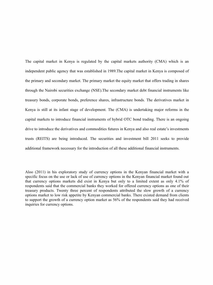
The capital market in Kenya is regulated by the capital markets authority (CMA) which is an

independent public agency that was established in 1989.The capital market in Kenya is composed of

the primary and secondary market. The primary market the equity market that offers trading in shares

through the Nairobi securities exchange (NSE).The secondary market debt financial instruments like

treasury bonds, corporate bonds, preference shares, infrastructure bonds. The derivatives market in

Kenya is still at its infant stage of development. The (CMA) is undertaking major reforms in the

capital markets to introduce financial instruments of hybrid OTC bond trading. There is an ongoing

drive to introduce the derivatives and commodities futures in Kenya and also real estate’s investments

trusts (REITS) are being introduced. The securities and investment bill 2011 seeks to provide

additional framework necessary for the introduction of all these additional financial instruments.

Aloo (2011) in his exploratory study of currency options in the Kenyan financial market with aspecific focus on the use or lack of use of currency options in the Kenyan financial market found outthat currency options markets did exist in Kenya but only to a limited extent as only 4.1% ofrespondents said that the commercial banks they worked for offered currency options as one of theirtreasury products. Twenty three percent of respondents attributed the slow growth of a currencyoptions market to low risk appetite by Kenyan commercial banks. There existed demand from clientsto support the growth of a currency option market as 56% of the respondents said they had receivedinquiries for currency options.

The Kenya shilling is usually very volatile hitting highs of 107 as it did in October 2011 whereas it has also hit lows of 61 in 2008.Most of the trading in imports and exports involve the dealing with theUSD and hence development of foreign currency options market will enable hedge against foreign exchange risk. Most of the trading in currency options in Kenya today is OTC by various commercial banks like the Kenya commercial bank and Commercial bank of Africa offer currency options but on a limited scale. Understanding the valuation of currency options will be important in development of an efficient currency options market in Kenya.

1.2. Statement of the Problem

There are two views in pricing of foreign currency options. One assumes that the volatility used in the

valuation of currency options is known and is constant and the other argues that volatility is

stochastic. Garman and Kohlhagen (1983) developed a variation of (B-S) used in the valuation of

currency options. Black and Scholes (1973) developed the landmark paper in valuation of options.

Most of pricing models today seek to relax the assumptions made by Black and Scholes (1973) and

most focus on stochastic volatility develop a model for predicting volatility which is then plugged into

the (B-S) model and Garman Kohlhagen Model.

Various studies have been done in Kenya relating to derivatives but most of the studies done so far have been exploratory in nature, Alaro (1998) studied the conditions necessary for the existence of a currency options market in Kenya. His study analyzed the conditions necessary for the operation of currency options by reviewingavailable literature. He concluded that main conditions for an options market to exist were a growing economy, supported by the Central Bank of Kenya, a fairly independent exchange rate mechanism, market liquidity and

efficiency, a regulatory organization and a strong and developing banking system. The study recommended the strengthening of the regulatory framework to provide clear guidelines as to the operation of currency option markets.

Aloo (2011)in his exploratory study of currency options in the Kenyan financial market with a

specific focus on the use or lack of use of currency options in the Kenyan financial market. The study

found that currency markets did exist in Kenya but only to a limited extent as only 4.1% of

respondents said that the commercial banks they worked for offered currency options as one of their

treasury products. Twenty three percent of respondents attributed the slow growth of a currency

options market to low risk appetite by Kenyan commercial banks. There existed demand from clients

to support the growth of a currency option market as 56% of the respondents said they had received

inquiries for currency options.Orina (2009) in a survey to a survey of the factors hindering the trading

of financial derivatives in the NSE found out that there existed factors of lack of adequate regulation

and lack of adequate demand that hindered the trading of financial derivatives at NSE.

In Kenya few researches have been done in the area of foreign currency options and the ones thathave been done are exploratory in nature. This research seeks to fill this research gap and show howforeign currency options can be priced in Kenya. This research will important especially now thatderivatives’ trading is being introduced in Kenya and it will offer useful insights into foreign currencyoptions pricing.

1.3.

Research Objectives

This research seeks to achieve the following key research objectives:

1. To develop an appropriate model for predicting volatility of USD/KSHS exchange rate. 2. To conduct variance analysis for USD/KSHS foreign currency options.

3. To value foreign currency options in Kenya using the predicted volatility values.

1.4 Significance of the Study

The research into valuation of foreign currency options in Kenya is very important in hedging against

foreign exchange risk exposures. Foreign currency exchange rates in Kenya are unpredictable and are

not stable due to the opening up of the foreign exchange market by the central bank. The exchange

rates are determined by the market hence foreign currency options will be of Importance to the

following: This research will use the USD/KSHS exchange rates.

The first are the importers who have to pay for their imports in the foreign currency and by the use of

the pricing framework brought by this foreign currency options pricing. Here the importers can first

buy a call option on the foreign currency which gives the importer the right to buy the foreign

currency at a certain fixed price. Under if the Kenya shilling depreciates against the USD the importer

exercises the call option to cover the downside risk and on the other hand if the Kenya shilling

appreciates against the USD the importer will exercise the put option then he can sell the currency in

the market at a higher rate and earn a profit.

Exporters on the other hand usually receive the payment for their exports in foreign currencyequivalent of their Kenya shillings price and here they can buy some call and put options.

Whereby if the Kenya shilling appreciates against the USD they will exercise the call options to coverthe downside risk and if the Kenya shilling depreciates they will exercise the put options on the USD so as to gain a profit.

Banks also will find this pricing framework very important as they will be able to offer new financialinstruments to their customers to hedge against foreign exchange risk by selling both call and putoptions on various currencies. Here the banks will be able to also hedge their downside risk relating toforeign currency and also profit at the same time.

CHAPTER TW

O

LITERATURE REVIEW

2.1 Introduction

This chapter seeks to analyze the literature relating to foreign currency options pricing. The chapter

will have three broad areas where various theories of foreign currency options will first be analyzed.

The chapter will show how the pricing of foreign currency options has evolved by analyzing three

theories of Black and Scholes (1973) model, Garman and Kohlhagen (1983) model and the binomial

option pricing model. Once the various theories of foreign currency option pricing have been

analyzed empirical studies will then be analyzed showing clearly findings of various researchers who

have ventured into the area of foreign currency option valuation.

The chapter will show clearly the various empirical findings done by the researchers in this area offoreign currency option pricing. The chapter will show clearly the different researches done and howthey differ from each other and also show the similarities of the various studies done by differentresearchers. The evolution of the research into the area of foreign currency pricing will be clearlystipulated showing how the valuation of foreign currency options has evolved from the seminal paperto date. Then finally the chapter will offer a conclusion that can be drawn from the literature reviewshowing what are the major themes of the literature on pricing of foreign currency options. Majorcontestations will also be spelt out in the literature review and research gaps identified.

2.2

Review of Theories

= d1 −σ

T ..............................................( vi )σ T

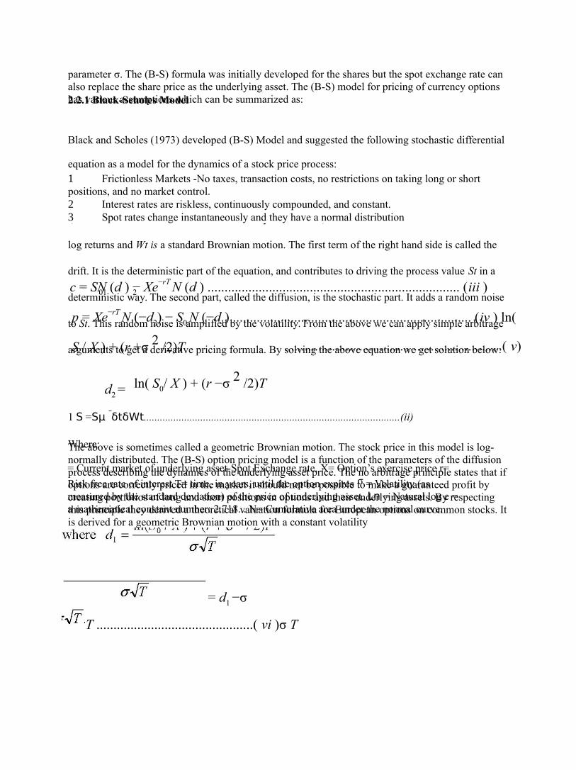
2.2.1 Black-Scholes Model

Black and Scholes (1973) developed (B-S) Model and suggested the following stochastic differential

equation as a model for the dynamics of a stock price process:

…………………………………………………………………. (i) Where St is the stock price at time

t, is the return on the stock and is the volatility of the stock, defined as the standard deviation of the

log returns and Wt is a standard Brownian motion. The first term of the right hand side is called the

drift. It is the deterministic part of the equation, and contributes to driving the process value St in a

deterministic way. The second part, called the diffusion, is the stochastic part. It adds a random noise

to St. This random noise is amplified by the volatility. From the above we can apply simple arbitrage

arguments to get a derivative pricing formula. By solving the above equation we get solution below:

1 S =Sµ δtδWt...............................................................................................(ii)

The above is sometimes called a geometric Brownian motion. The stock price in this model is log-normally distributed. The (B-S) option pricing model is a function of the parameters of the diffusion process describing the dynamics of the underlying asset price. The no arbitrage principle states that if options are correctly priced in the market it should not be possible to make a guaranteed profit by creating portfolios of long and short positions in options and their underlying assets. By respecting this principle they derived a theoretical valuation formula for European options on common stocks. It is derived for a geometric Brownian motion with a constant volatility

parameter σ. The (B-S) formula was initially developed for the shares but the spot exchange rate can also replace the share price as the underlying asset. The (B-S) model for pricing of currency options has various assumptions which can be summarized as:

1 Frictionless Markets -No taxes, transaction costs, no restrictions on taking long or short positions, and no market control. 2 Interest rates are riskless, continuously compounded, and constant. 3 Spot rates change instantaneously and they have a normal distribution

c = SN (d ) − Xe−rT N (d ) .......................................................................... (iii )01 2

p = Xe−rT N (−d2) − S0 N (−d1) ...................................................................... (iv ) ln(

S / X ) + (r +σ 2 /2)T ................................................................( v)

ln( S0/ X ) + (r −σ 2 /2)Td2 =

Where:

= Current market of underlying asset-Spot Exchange rate. X= Option’s exercise price r=

Risk free rate of interest T= time, in years, until the option expires σ = Volatility (as measured by the standard deviation) of the price of underlying asset. Ln = Natural log e =a mathematical constant number: 2.718... N= Cumulative area under the normal curve.

For the Black-Scholes model, the only input that is unobservable is the future volatility of the underlying asset. One way to determine this volatility is to select a value that equates the theoretical (B-S) price of the option to the observed market price. This value is often referred to as the implied orimplicit volatility of the option. Under the (B-S) model implied volatilities from options should be thesame regardless of which option is used to compute the volatility.

2.2.2 Garman and Kohlhagen model

Garman and Kohlhagen (1983) extended the Black Scholes model to cover the foreign exchange

market, Garman and Kohlhagen suggested that foreign exchange rates could be treated as non-

dividend paying stocks. Where they allowed for the fact that currency pricing involves two interest

rates and that a currency can trade at a premium or discount forward depending on the interest rate

differential. The Garman and Kohlhagen formula applies only to European options. Garman and

Kohlhagen (1983) extended the (B-S) to cope with the presence of two interest rates the domestic

interest rate and the foreign currency interest rate.

The model assumed that It is easy to convert the domestic currency into the foreign currency and thatwe can invest in foreign bonds without any restrictions. The standard Garman and Kohlhagen foreigncurrency option pricing model has the following form:

-

…………………………………………………. (vii)

+ ………………………………………… (viii) Where:

= …………………………………………………………… (ix) √

√

…

…

…

…

…

…

…

…

…

…

…

…

…

…

…

…

…

…

…

…

…

…

…

…

…

…

…

(x)

And,

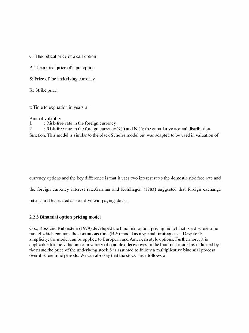
C: Theoretical price of a call option

P: Theoretical price of a put option

S: Price of the underlying currency

K: Strike price

t: Time to expiration in years σ:

Annual volatility 1 : Risk-free rate in the foreign currency 2 : Risk-free rate in the foreign currency N( ) and N ( ): the cumulative normal distribution function. This model is similar to the black Scholes model but was adapted to be used in valuation of

currency options and the key difference is that it uses two interest rates the domestic risk free rate and

the foreign currency interest rate.Garman and Kohlhagen (1983) suggested that foreign exchange

rates could be treated as non-dividend-paying stocks.

2.2.3 Binomial option pricing model

Cox, Ross and Rubinstein (1979) developed the binomial option pricing model that is a discrete time model which contains the continuous time (B-S) model as a special limiting case. Despite its simplicity, the model can be applied to European and American style options. Furthermore, it is applicable for the valuation of a variety of complex derivatives.In the binomial model as indicated by the name the price of the underlying stock S is assumed to follow a multiplicative binomial process over discrete time periods. We can also say that the stock price follows a

random walk, because in each period, it may either move up by a certain percentage amount u-1 where u > 1 or down by a certain percentage amount 1 -d where d < 1. We denote the (physical) probability of an upward move as

p

and the (physical) probability of a downward move as 1 -

p

. Let

be the current value of a European style option, whereas f can be either a call (

) or a put (

) option. Then

(

or

) is the option's price if the stock price moves upward, and

(

or

its price if the stock price moves downward:

With probability p

With probability 1 -p

If the call option is only away one period from expiration, Then ( orand ( or are given by = max ( u -K; 0) or = max (K - u; 0); = max ( d -K; 0) or = max (K - d; 0);

2.3

Review of Empirical Studies

Fabozzi, Hauser and Yaari (1990) conducted a research that compared the performance of the Barone

Adesi Whaley (BA-W) model for currency options and Garman Kohlhagen model in pricing

American currency options. It was shown that the (BA-W) model is superior to the Garman

Kohlhagen model in pricing out-of-the-money long-term put options and inferior in pricing in-the-

money short-term put options. The two models performed equally well in pricing call options. The

research further shown that the interest rate differential across countries has a greater effect on the

probability of gainful early exercise in foreign currency puts than that of calls. The American model

identified a large number of opportunities in our sample for gainful early exercise among in-the-

money options maturing in less than 45 days. These findings suggest the need for a further

investigation of the ex-post consequences of early exercise decisions based on the (BA-W) model. In

combination with our results, such an investigation was found to be useful in the developments of

trading strategies and the testing of market efficiency.

Campa and Chang (1995, 1998) conducted a research to test the suitability of the (B-S) model argue

that the (B-S) model generates accurate option values even though it may be misspecified,and use (B-

S) implied volatilities to forecast exchange rate variance and the correlations between exchange rates.

Hamilton and Susmel (1994) present a regime switching model in which each regime is characterized by a different ARCH process. In their model, the null of a single regime would be equivalent to a single ARCH process governing innovations. In this sense their regime switching model nests a standard ARCH process. However, as Hamilton and Susmel point out, the general

econometric problem of regime switching models remains: the null of a single regime is not testable in the usual way since parameters of the other regimes are not identified. Hamilton and Susmel rely on standard linear regression statistics as a simple measure of relative fit.

Bollen et al (2003) compares the performance of three competing option valuation models in the

foreign exchange market, one based on a regime-switching process for exchange rate changes, one

based on a GARCH process, and the other based on jump diffusion. Three tests are executed based on

the parameter values implicit in option prices. The first test compares in sample fit of option prices.

The study found out that GARCH model is superior to the regime-switching model for the GBP, but

the two models perform about the same for the JPY. Both models dominate an ad hoc valuation model

based on Black Scholes, but both are dominated by the jump diffusion model. The second test

compares out-of-sample fit of option prices. Here the GARCH model performs better than the

regime-switching model for both exchange rates, and again both are superior to an ad hoc valuation

model. The jump-diffusion model offers only modest improvement over the others for the GBP

options. The third test simulates the role of a market maker who sells options and uses the competing

valuation models to hedge the positions. In this test, the GARCH and regime-switching models

perform almost identically. An ad hoc strategy is superior for the GBP and is inferior for the JPY. The

jump-diffusion model performs as well as the ad-hoc strategy for the GBP and is superior to all others

for the JPY options.

Kalivas and Dritsakis (1997) in their study dealing with volatility forecasting techniques and volatilitytrading in the case of currency options they sought to provide evidence on how foreign exchange ratesare moving under time varying volatility. They sought to identify the existence of

heteroscedasticity then applied widely acclaimed methods in order to estimate future exchange rates under changing volatility. They then used different methods for estimating future foreign exchange volatility, such as implied volatility and historical volatility approaches.In their study implied and historical volatility were compared and it was found, that historical volatility is the best approximation. The white

’

s test for existence of heteroscedasticity showed that there was time variation in volatility.

Abken and Nandi (1996) model the volatility in such a way that the future volatility depends on a

constant and a constant proportion of the last period’s volatility. They used the ARCH framework to

predict volatility.Thus, ARCH models provide a well-established quantitative method for estimating

and updating volatility.

Natenberg (1994) proposed a forecast by using a weighting method, giving more distant volatility

data progressively less weight in the forecast. The above weighting characteristic is a method which

many traders and academics use to forecast volatility. It depends on identifying the typical

characteristics of volatility, and then projecting volatility over the forecasting period.

Melino and Turnbull (1990) found that the stochastic volatility model dominates the standard option valuation models. In addition, they pointed out that a stochastic volatility model yield option prices which coincide with the observed option prices market prices.They generalized the model to allow stochastic volatility and they report that this approach is successful in explaining the prices of currency options. Though this model has the disadvantage that their models do not

have closed form solutions and require extensive use of numerical techniques to solve two dimensional partial differential equations.

Scott and Tucker (1989) examined the relative performance of three different weighting schemes for

calculating implied volatility from American foreign exchange call options on the British pound,

Canadian dollar, Deutschemark, Yen; and Swiss franc. They found no evidence that one of the three

weighting schemes is superior to the others.

Kroner et al. (1995) found out implied volatility being higher than historical volatility due to the fact

that if interest rates are stochastic, then the implied volatility will capture both asset price volatility

and interest rate volatility, thus skewing implied volatility upwards, and that if volatility is stochastic

but the option pricing formula is constant, then this additional source of volatility will be picked up by

the implied volatility.Kroner et al (1995) also point out that, since expectations of future volatility

play such a critical role in the determination of option prices, better forecasts of volatility should lead

to a more accurate pricing and should therefore help an option trader to identify over-or underpriced

options. Therefore a profitable trading strategy can be established based on the difference between the

prevailing market implied volatility and the volatility forecast.

Dontwi, Dedu and Biney (2010)in pricing of foreign currency options in a developing financial Market. They conducted a research seeking to develop a suitable approach to the valuation of foreign currency options in an underdeveloped financial market in Ghana. Volatility analysis was done. This included the application of the GARCH model which resulted in the marginal

volatility measure. Further, the pricing of basic foreign currency options in the local market was obtained from the marginal volatility measure. The research had the following findings and conclusions: The resulting GARCH specification volatility measure can then be implemented as an input in the pricing of theoretically formed currency options in the local market. This analysis can form the basis for the pricing of currency options in developing financial the local markets. Implementation of the standardized instruments is expected to follow the further development of the domestic Forex market, its size, liquidity and legislative framework. In the beginning the further Pricing of Foreign Currency Options in a Developing Financial Market implementation of forward and swap contracts is appropriate, until the volume of trading reaches levels That would require standardization of contracts and their variety. More complex pricing schemes would then be available and adequate Forex management schemes created. This opens avenue for further research directions.

Heston (1993) proposed a closed form solution for options with stochastic volatility with applications to bond and currency options where he used a new technique to derive a closed-form solution for the price of a European call option on an asset with stochastic volatility. The model allows arbitrary correlation between volatility and spot asset returns. He introduced stochastic interest rates and showshow to apply the model to bond options and foreign currency options. Simulations show that correlation between volatility and the spot asset’s price is important for explaining return skewness and strike-price biases in the Black Scholes (1973) model. The solution technique is based on characteristic functions and can be applied to other problems.

Chen and Gau (2004) investigates the relative pricing performance between constant volatility and stochastic volatility pricing models, based on a comprehensive sample of options on four currencies, including the British pound, Deutsche mark, Japanese yen and Swiss franc, traded frequently in the Philadelphia Stock Exchange (PHLX) from 1994 to 2001. The results show that Heston model outperforms the (G-S) model in terms of sum of squared pricing errors for all currency options and the adjustment speed toward the long-run mean volatility in the currency market is faster than that in the stock market.

Posedel (2006) analyzed the implications of volatility that changes over time for option pricing. The

nonlinear-in-mean asymmetric GARCH model that reflects asymmetry in the distribution of returns

and the correlation between returns and variance is recommended. He used the NGARCH model for

the pricing of foreign currency options. Possible prices for such options having different strikes and

maturities are then determined using Monte Carlo simulations. The improvement provided by the

NGARCH model is that the option price is a function of the risk premium embedded in the

underlying asset. This contrasts with the standard preference-free option pricing result that is obtained

in the Black-Scholes model.

Aloo (2011)in his exploratory study of currency options in the Kenyan financial market with a specific focus on the use or lack of use of currency options in the Kenyan financial market. The study found that currency markets did exist in Kenya but only to a limited extent as only 4.1% of respondents said that the commercial banks they worked for offered currency options as one of their treasury products. Twenty three percent of respondents attributed the slow growth of a currency options market to low risk appetite by Kenyan commercial banks. There existed

demand from clients to support the growth of a currency option market as 56% of the respondents said they had received inquiries for currency options.

Akinyi (2007) did a study where she compared the classical B-S model and the Garch option pricing

model in Kenya and she looked at the consequences of introducing heteroscedasticity in option

pricing. The analysis showed that introducing heteroscedasticity results in a better fitting of the

empirical distribution of foreign exchange rates than in the Brownian model. In the Black-Scholes

world the assumption is that the variance is constant, which is definitely not the case when looking at

financial time series data. The study priced a European call option under a Garch model Framework

using the Locally Risk Neutral Valuation Relationship. Option prices for different spot prices are

calculated using simulations. The study used the non-linear in mean Garch model in analyzing the

Kenyan foreign exchange market.

2.4 Conclusion from literature review

The original option pricing model was developed by Black and Scholes (1973). Since then, it hasbeen extended to apply to foreign currency options in Garman and Kohlhagen, 1983; Grabbe, (1986).Garman and Kohlhagen (1983) suggested that foreign exchange rates could be treated as non-dividend-paying stocks. From the initial studies of foreign currency option valuation variousassumptions were made by Black and Scholes (1973) and research from that time has been focused ofrelaxing some of the assumptions. From the literature volatility is the main variable involved whereby most researchers now focus on developing a model of predicting future volatility based on eitherhistorical data or implied volatility.

Volatility forecasts have many practical applications such as use in the analysis of market timing decisions, aid with portfolio selection and the provision of estimates of variance for use in option pricing models. Thus, it follows that it is important to distinguish between various models in order to find the model which provides the most accurate forecast the literature provides conflicting evidence about the superiority of each method. One the one hand, some researchers stress that relatively complex forecasts (ARCH) and (GARCH) models and implied volatility forecasts provide estimationswith the best quality. From the literature review we can conclude that most of the models of option pricing are based on the initial model of Black and Scholes and almost all the models start there and go on and relax some of the unrealistic assumptions made by the black Scholes model of option pricing. In general we can say that Black & Scholes assumed that the financial market is a system thatis in equilibrium. Most research on pricing of currency options have concentrated in developed markets and there is a research gap to conduct research in valuation of developing and emerging markets like the Kenya market. The financial markets of developed countries where most of the research on the valuation of foreign currency options has been carried out is different from the financial market in Kenya in terms of efficiency and the way they are structured .Also there is currently no market for trading of options in Kenya and some data used in the model is not readily available as in the developed financial markets. Due to the above differences in the financial markets in developed economies and Kenya

’

s financial market there is need to come up with a model that properly fits the available data in Kenya hence the model developed specifically for Kenya will give more accurate results in valuation of foreign currency options in Kenya compared to using the already developed models for developed countries.

CHAPTER THRE

E

RESEARCH METHODOLOGY

3.1 Introduction

This chapter discusses the type of research methodology used in the study. First the research design used is discussed and it’s very important to select the appropriate research design as this will enable you to achieve the research objectives. The population of the study is then defined and the sample thatwill be used is then selected and justified. Data collection methods and data analysis methods that willbe used are then discussed. Then the conceptual and empirical models are then defined and various variables defined and then finally the data validity and reliability is explained.

3.2 Research design

Research design refers to how data collection and analysis are structured in order to meet the research

objectives through empirical evidence economically Schindler (2006). This research uses descriptive

research design which is a scientific method which involves observing and describing the behavior of

a subject without influencing it in any way. The research looks at USD/KSHS exchange rate in the

past and analyses it to come up with a pricing model for foreign currency options in Kenya.

3.3 Population

Cooper and Emory (1995) define population as the total collection of elements about which the researcher wishes to make inferences. The population of interest in this study is the foreign currency exchange rates in Kenya.

3.4

Sample

The sample for this research will be the daily USD/KSHS exchange rate for 5 years from 2008 to

2012.The exchange rates used in formulating the model for predicting volatility are the mean daily

exchange rates from January 2008 to December 2012 with 1253 daily data exchange rates for the

USD against the KSHS. The exchange rate for the USD against the Kenya Shilling range from a low

of 61.51 in May 2008 to a high of 105.91 in October 2011 but the majority of the exchange rates lie

between 70-90 against the USD. For the simulation of the foreign currency option pricing exchange

rate data for January 2013 is used. The USD is used for it’s the most traded currency and most

transactions in Kenya are pegged against the USD which also acts as the intermediary in triangular

currency transactions. The exchange rates are given by appendix 3.

3.5 Data Collection

This study will use secondary data for the various variables that will be put into the model. Thesecondary data will be obtained from Central bank of Kenya and Kenya bureau of statistics. Thesecondary data collected will cover a period of five years from 2008 to 2012.

3.6 Data Analysis

This study will use both descriptive and inferential statistics to analyze the data. Analysis will be doneusing the Statistical package for social scientists (SPSS Version 20).Secondary data will be collectedthen regression analysis will be carried out to model the volatility equation and the gained volatilityestimate used in the valuation of foreign currency options.

3.7

Conceptual model

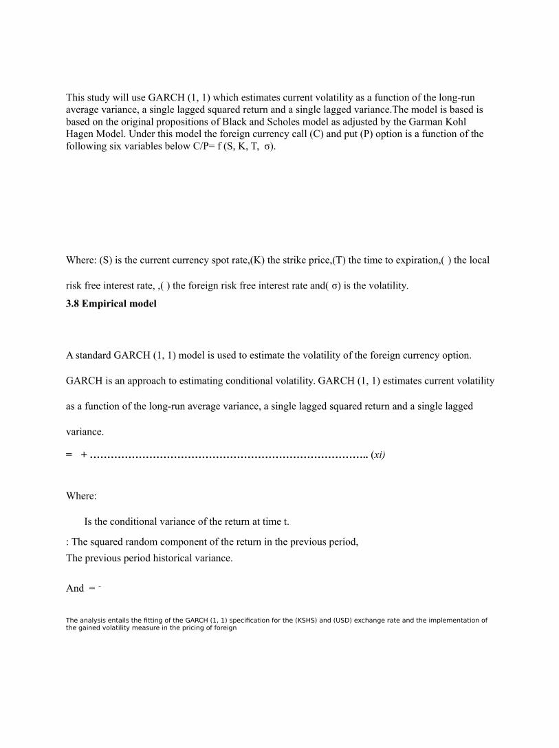
This study will use GARCH (1, 1) which estimates current volatility as a function of the long-run average variance, a single lagged squared return and a single lagged variance.The model is based is based on the original propositions of Black and Scholes model as adjusted by the Garman Kohl Hagen Model. Under this model the foreign currency call (C) and put (P) option is a function of the following six variables below C/P= f (S, K, T, σ).

Where: (S) is the current currency spot rate,(K) the strike price,(T) the time to expiration,( ) the local

risk free interest rate, ,( ) the foreign risk free interest rate and( σ) is the volatility.

3.8 Empirical model

A standard GARCH (1, 1) model is used to estimate the volatility of the foreign currency option.

GARCH is an approach to estimating conditional volatility. GARCH (1, 1) estimates current volatility

as a function of the long-run average variance, a single lagged squared return and a single lagged

variance.

= + …………………………………………………………………….. (xi)

Where:

Is the conditional variance of the return at time t.

: The squared random component of the return in the previous period,

The previous period historical variance.

And =

The analysis entails the fitting of the GARCH (1, 1) specification for the (KSHS) and (USD) exchange rate and the implementation of the gained volatility measure in the pricing of foreign

currency options in the Kenyan market. Once the variance is estimated standard deviation which represents the volatility is attained by finding the square root of the variance. The volatility is estimated on monthly basis and is assumed to be constant over that month. The above volatility model is used to predict volatility for the next period which is the month that follows .The volatility will bepredicted by the above model then the resultant volatility plugged into the Garman and Kohlhagen model stipulated below. All the variables below are observable except volatility which will be estimated from the above model.

- ……………………………………………………… (vii)

+ ……………………………………………… (viii) Where:

= √

……………………………………………………………….. (xi)

√…………………………………………………………………………. ..(x) And,

C: theoretical price of a call option

P: theoretical price of a put option

S: price of the underlying currency

K: strike price-(Simulated values are used).

t: time to expiration in years

σ: annual volatility 1 : The risk-free rate in the foreign currency 2 The risk-free rate in the Kenya economy.

N(

) and N (

): the cumulative normal distribution function All the above variables are observable except annual volatility which will be estimated by the Garch (1, 1) model above and the foreign currency call and put options will be valued at various simulated strike prices.

3.9 Data Validity & Reliability

The data validity and reliability will be assured for this study will use secondary data from trusted sources of Central bank of Kenya and the Kenya national bureau of statistics.

CHAPTER FOU

R

DATA ANALYSIS AND PRESENTATION

4.1 Introduction

This of data analysis and presentations has two major parts. First the data is clearly presented and

defined, data analysis methods used for the research is also discussed and finally summary and

findings are clearly interpreted.

4.2 Data Presentation

4.2.1 Variance

The variance is a measure of the squared deviations of the observations from the mean. In this

research first price relatives are calculated from the exchange rates given, then natural logs of the

price relatives are now used as the variable by which the variance is estimated. In this research

variance is assumed to follow an historical trend where the variance of today’s period determines the

variance of the following periods. The variance in this research is a function of two main dependent

variable whereby current period’s variance depends on previous period variance and previous period

squared log returns. The variance used in the study is the historical variance which is calculated based

on the returns of the USD/KSHS exchange rates and the variance period is thirty days.

4.2.2 Squared log Returns

Squared log returns is one of the independent variable is this research. For this research squared log returns for the exchange rates is used to estimate variance and consequently the volatility. The squared log returns has been determined to be a goon variable for estimating the variance

from previous studies done in this area of pricing of foreign currency options. To determine the squared log returns first the exchange price relative rates is calculated and the price relative relates thecurrent daily exchange rate with the previous day's exchange rate and it

’

scomputed by dividing current daily exchange rate by the previous day exchange rate. The squared log returns is based on the natural logarithm of price relative of the USD/KSHS exchange rates as illustrated in appendix 1.

4.2.3 Risk free rate

Risk free interest rate is the theoretical rate of return of an investment with zero risk including the

default risk. The risk free rate represents the interest that an investor would expect from an absolutely

risk free investment over a given period of time.Risk free rate can be said to be the rate of interest

with no risk. Therefore any rational investor will reject all the investments yielding sub risk free

returns.The risk free rate is usually obtained from government securities which offer a guaranteed

return with no risk. The risk free rates used are the 364 days Treasury bill rate for the domestic Kenya

interest rate which in January 2013 averaged 11.67% and the foreign risk free rate the 1 year Treasury

bill for USA was used in the study and the foreign risk free rate is as shown in appendix 2.

4.2.4 Strike price

The strike price is defined as the price at which the holder of currency options can buy in the case of acall option or sell in the case of a put option the underlying security when the option is exercised. Since we don’t have the options market in Kenya the foreign currency options was priced based on simulated strike prices of 70,80,90 and 100.These four strike prices are adequate in this analysis as they help portray various pricing dynamics of foreign currency options

pricing.The strike prices selected will be adequate in illustrating the pricing of foreign currency options the exchange rate for the USD versus the Kenya shilling is usually within this range.

4.2.5 Time to maturity

The time to maturity is the period that remaining before the option expires. This research assumes that

the currency options are European currency options that can only be exercised on the maturity date on

their expiry date. The time to maturity used in this study is a foreign currency option of 6 months and

this translates to a 0.5 fraction of a year.

4.2.6 Volatility

Volatility is one of the major variable in this research and coming up with a good volatility estimate isvery key in coming up with an adequate and accurate foreign currency pricing model. Volatilityshowsthe variation in data in relation to the mean. If the data is close together, the standard deviation will besmall. If the data is spread out, the standard deviation will be large. Volatility is estimated from asample of recent continuously compounded returns .This research uses historical volatility estimatesand assumes that volatility of the past will hold in the future and in this research variance from pastdata of the exchange rates for the USD against the Kenya shilling is calculated and a regression modelbased on the Garch (1, 1) framework is formulated to predict future volatility. From the predictedvariance estimates we obtain the standard deviation by finding the square-root of the estimatedvariance which represents the volatility used in pricing of foreign currency options. The volatility usedin this study is as predicted by the variance model and it’s shown in appendix 2

4.3

Regression results analysis and application of model.

Regression analysis was conducted for the above model and produced the following resultssummarized below.

ModelR R Square

Adjusted R Square

Std. Error of theEstimate

1 .995a .990 .990 .000005765254121

Table 1:Model Summary

Predictors: , ,

Dependent Variable:

R square is the coefficient of determination and shows by what proportion the variations of the dependent variable are explained by the independent variables. From above the R Square statistic gives the goodness of fit of the model which shows how good the regression model approximates the real data points. An R square of 1.0 indicates that the regression line perfectly fits the data. The R square of this model is .990 which shows that the model is a good fit of the actual data. Coefficient of correlation ranges between -1 to 1 and in this model the coefficient of correlation is .995 which shows a high positive correlation between current period variance, previous period variance and previous period log returns.

Table 2:Coefficients

Model Coefficients T Sig.

B Std. Error

4.153E-007 .968 .012

.000 .003 .002

2.139 321.410 6.589

.033 .000 .000

Dependent Variable:

Independent variable:,

From above the analysis of the data a variance model can be fitted for the exchange rate data of USD

against Kenya Shilling. From the coefficients obtained above we have the following variance model

which satisfies the Garch (1, 1) conditions as (+) <1.

= 0.0000004153+0.968 +0.012

The above model is the model that is used to predict variance then we find the square root of the

estimated variance to get the standard deviation which will be used as the volatility in the Garman

Kohlhagen model as illustrated below.

By use of simulation for a hypothetical foreign currency call and put option can be valued as shownbelow. Since strike price data is not available valuation of the currency option can be valued under forstrike prices of 70, 80, 90 and 100 exchange rates for the USD. January 2013 USD/KSHS exchangerates are used to generate the variables inputted in the variance model which is used to estimatevolatility for the period of January 2-15.

Table 3: Strike price at 70.

K=70

Date-January 2013

Exchange Rate (S)

σ% 364 day T-Bill -CBK

T Call Price

Put price

2 86.0769 1.733955898

11.67% 15%

0.5

13.82490236

9.2527E-56

3 86.3569 1.735499828

11.67% 15%

0.5

14.08467053

1.78183E-57

4 86.4417 2.138661907

11.67% 15%

0.5

14.16334318

3.64191E-39

7 86.4264 2.157175963

11.67% 15%

0.5

14.1491487

1.77897E-38

8 86.4775 2.161130222

11.67% 14%

0.5

14.59870562

2.04321E-40

9 86.5242 2.160869074

11.67% 13%

0.5

15.04663167

1.55639E-42

10 86.6053 2.15883403

11.67% 14%

0.5

14.71786555

4.70173E-41

First for the analysis of the model in practice first we look at the foreign currency option having astrike price of 70.The strike price of 70 is below the spot exchange rates which are above 86 for thesimulation period of January 2013 and hence its advantageous for the currency call holders to exercisethe calls as they would gain while for put holders they would lose out hence no put holder wouldexercise their put currency options. For this reason based on the laws of demand and supply andpractical options trading we have a higher demand for currency call options hence the higher pricecompared to the currency put options. The price of the currency call option ranges between 13.82-15.04 while the currency put option prices for this period of simulation are statistically Zero as shownin the above table.

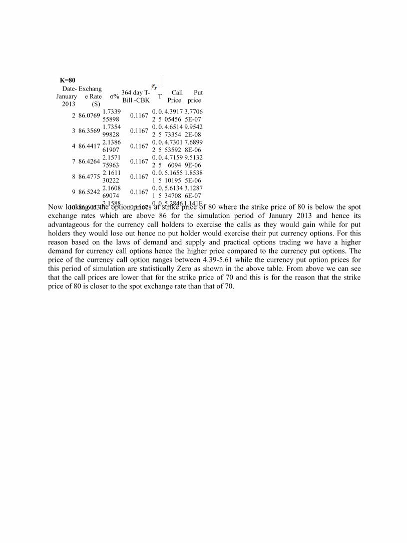
Table 4: Strike price at 80.

K=80 Date-

January2013

Exchange Rate

(S) σ%

364 day T-Bill -CBK

T Call

Price Put

price

2 86.0769 1.733955898

0.1167 0.2

0.5

4.391705456

3.77065E-07

3 86.3569 1.735499828

0.1167 0.2

0.5

4.651473354

9.95422E-08

4 86.4417 2.138661907

0.1167 0.2

0.5

4.730153592

7.68998E-06

7 86.4264 2.157175963

0.1167 0.2

0.5

4.71596094

9.51329E-06

8 86.4775 2.161130222

0.1167 0.1

0.5

5.165510195

1.85385E-06

9 86.5242 2.160869074

0.1167 0.1

0.5

5.613434708

3.12876E-07

10 86.6053 2.1588

0.1167 0. 0. 5.2846 1.141ENow looking at the option prices at strike price of 80 where the strike price of 80 is below the spot

exchange rates which are above 86 for the simulation period of January 2013 and hence itsadvantageous for the currency call holders to exercise the calls as they would gain while for putholders they would lose out hence no put holder would exercise their put currency options. For thisreason based on the laws of demand and supply and practical options trading we have a higherdemand for currency call options hence the higher price compared to the currency put options. Theprice of the currency call option ranges between 4.39-5.61 while the currency put option prices forthis period of simulation are statistically Zero as shown in the above table. From above we can seethat the call prices are lower that for the strike price of 70 and this is for the reason that the strikeprice of 80 is closer to the spot exchange rate than that of 70.

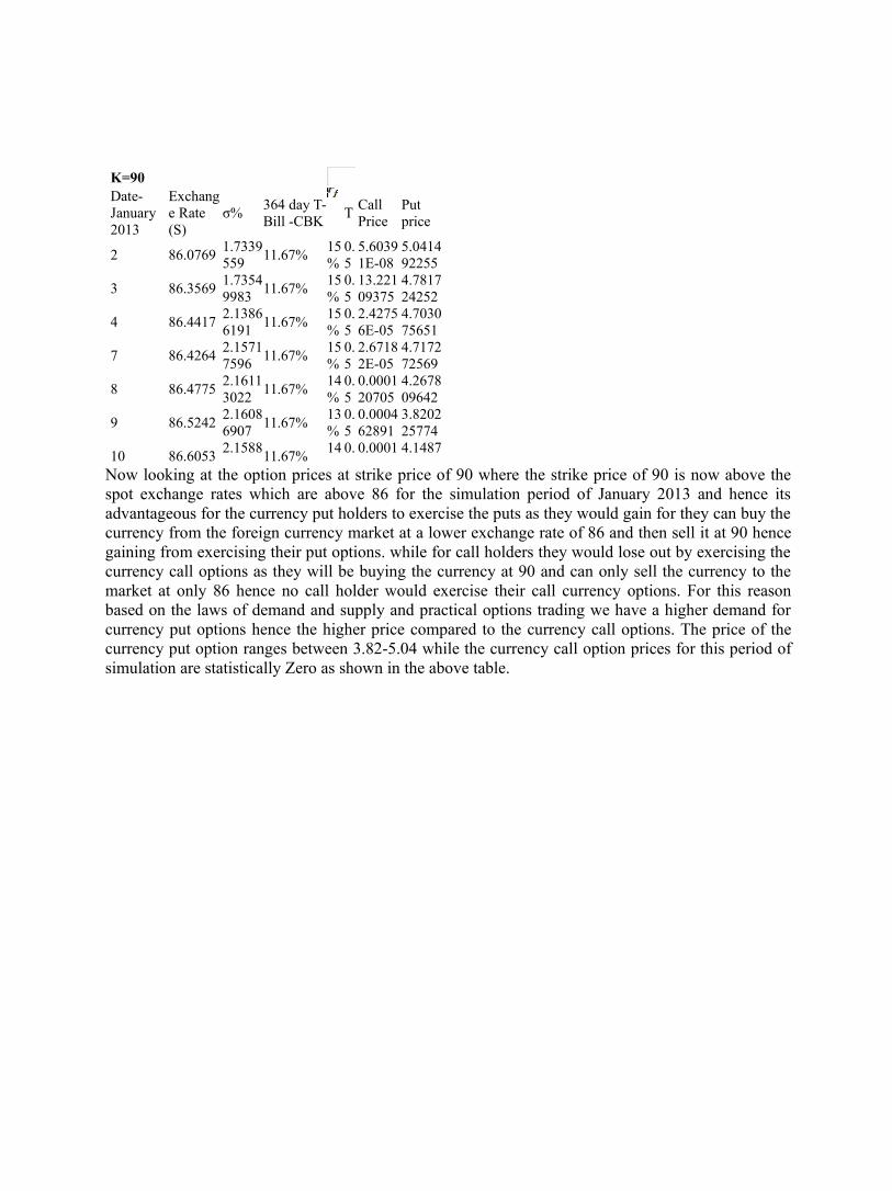
Table 5: Strike price at 90.

K=90 Date-January 2013

Exchange Rate (S)

σ% 364 day T-Bill -CBK

T Call Price

Put price

2 86.0769 1.7339559

11.67% 15%

0.5

5.60391E-08

5.041492255

3 86.3569 1.73549983

11.67% 15%

0.5

13.22109375

4.781724252

4 86.4417 2.13866191

11.67% 15%

0.5

2.42756E-05

4.703075651

7 86.4264 2.15717596

11.67% 15%

0.5

2.67182E-05

4.717272569

8 86.4775 2.16113022

11.67% 14%

0.5

0.000120705

4.267809642

9 86.5242 2.16086907

11.67% 13%

0.5

0.000462891

3.820225774

10 86.6053 2.1588

11.67% 14 0. 0.0001 4.1487

Now looking at the option prices at strike price of 90 where the strike price of 90 is now above thespot exchange rates which are above 86 for the simulation period of January 2013 and hence itsadvantageous for the currency put holders to exercise the puts as they would gain for they can buy thecurrency from the foreign currency market at a lower exchange rate of 86 and then sell it at 90 hencegaining from exercising their put options. while for call holders they would lose out by exercising thecurrency call options as they will be buying the currency at 90 and can only sell the currency to themarket at only 86 hence no call holder would exercise their call currency options. For this reasonbased on the laws of demand and supply and practical options trading we have a higher demand forcurrency put options hence the higher price compared to the currency call options. The price of thecurrency put option ranges between 3.82-5.04 while the currency call option prices for this period ofsimulation are statistically Zero as shown in the above table.

Table 6: Strike price at 100.

K=100 Date-January 2013

Exchange Rate (S)

σ% 364 day T-Bill -CBK

T Call Price

Put price

2 86.0769 1.733955898

11.67% 15% 0.5 1.87413E-43

14.4747

3 86.3569 1.735499828

11.67% 15% 0.5 8.08449E-42

14.2149

4 86.4417 2.138661907

11.67% 15% 0.5 4.17392E-28

14.1362

7 86.4264 2.157175963

11.67% 15% 0.5 1.01088E-27

14.1504

8 86.4775 2.161130222

11.67% 14% 0.5 6.15026E-26

13.7009

9 86.5242 2.160869074

11.67% 13% 0.5 2.53207E-24

13.253

10 86.6053 2.15883403

11.67% 14% 0.5 1.50311E-25

13.5817

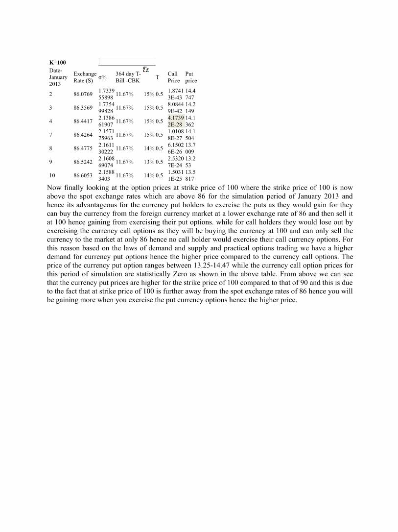
Now finally looking at the option prices at strike price of 100 where the strike price of 100 is nowabove the spot exchange rates which are above 86 for the simulation period of January 2013 andhence its advantageous for the currency put holders to exercise the puts as they would gain for theycan buy the currency from the foreign currency market at a lower exchange rate of 86 and then sell itat 100 hence gaining from exercising their put options. while for call holders they would lose out byexercising the currency call options as they will be buying the currency at 100 and can only sell thecurrency to the market at only 86 hence no call holder would exercise their call currency options. Forthis reason based on the laws of demand and supply and practical options trading we have a higherdemand for currency put options hence the higher price compared to the currency call options. Theprice of the currency put option ranges between 13.25-14.47 while the currency call option prices forthis period of simulation are statistically Zero as shown in the above table. From above we can seethat the currency put prices are higher for the strike price of 100 compared to that of 90 and this is dueto the fact that at strike price of 100 is further away from the spot exchange rates of 86 hence you willbe gaining more when you exercise the put currency options hence the higher price.

4.4

Summary and Interpretation of Findings

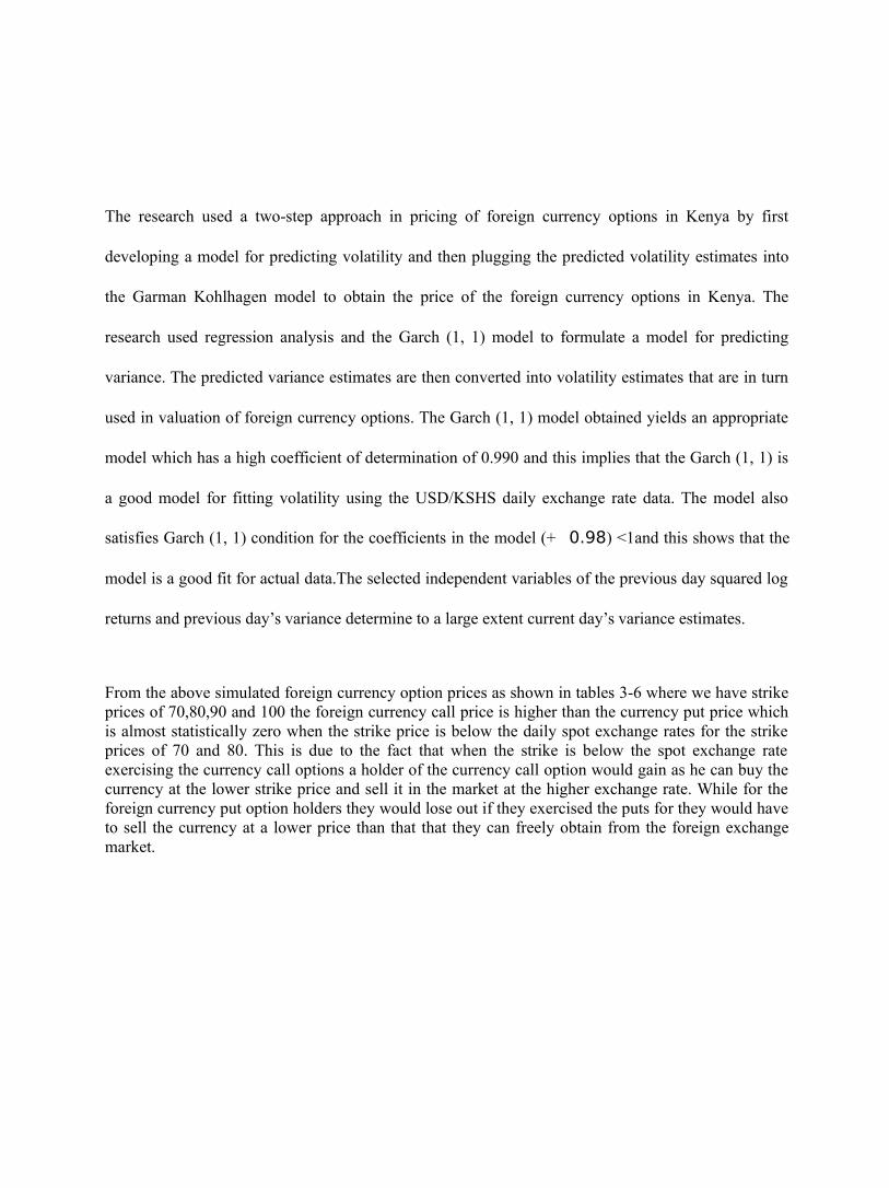
The research used a two-step approach in pricing of foreign currency options in Kenya by first

developing a model for predicting volatility and then plugging the predicted volatility estimates into

the Garman Kohlhagen model to obtain the price of the foreign currency options in Kenya. The

research used regression analysis and the Garch (1, 1) model to formulate a model for predicting

variance. The predicted variance estimates are then converted into volatility estimates that are in turn

used in valuation of foreign currency options. The Garch (1, 1) model obtained yields an appropriate

model which has a high coefficient of determination of 0.990 and this implies that the Garch (1, 1) is

a good model for fitting volatility using the USD/KSHS daily exchange rate data. The model also

satisfies Garch (1, 1) condition for the coefficients in the model (+ 0.98) <1and this shows that the

model is a good fit for actual data.The selected independent variables of the previous day squared log

returns and previous day’s variance determine to a large extent current day’s variance estimates.

From the above simulated foreign currency option prices as shown in tables 3-6 where we have strikeprices of 70,80,90 and 100 the foreign currency call price is higher than the currency put price whichis almost statistically zero when the strike price is below the daily spot exchange rates for the strikeprices of 70 and 80. This is due to the fact that when the strike is below the spot exchange rateexercising the currency call options a holder of the currency call option would gain as he can buy thecurrency at the lower strike price and sell it in the market at the higher exchange rate. While for theforeign currency put option holders they would lose out if they exercised the puts for they would haveto sell the currency at a lower price than that that they can freely obtain from the foreign exchangemarket.

When the strike price is above the daily spot exchange rate as shown in tables 5 and 6 the foreign currency options the foreign currency put price is higher than the currency call price which is almost statistically zero when the strike price is above the daily spot exchange rates for strike prices of 90 and 100. This is due to the fact that when the strike is above the spot exchange rate exercising the currency put options a holder of the currency put option would gain as he can buy the currency at the lower spot exchange rate and sell it at the higher spot exchange rate. While for the foreign currency call option holders they would lose out if they exercised the calls for they would have to pay more than the market spot exchange rate for the currencyand hence they would not exercise them.

From above simulation as shown in tables 3, 4, 5 and 6 using January 2013 USD/KSHS exchange ratedata foreign currency options can be valued in Kenya and the results obtained show that the valuationis consistent with previous literature and studies done on the valuation of foreign currency optionsespecially the studies that used the GARCH pricing like inDontwi, Dedu and Biney (2010)in pricingof foreign currency options in a developing financial Market in Ghana. The exchange rates betweenJanuary 2-15 range between 86.0769-86.6853 and using the strike prices of 70, 80, 90 and 100 thisstudy yields results consistent with previous theories and literature. From theory and previous studiesdone in the area of currency options valuation for call options, the higher the strike price, the cheaperthe currency call option and for put option the lower the strike price the cheaper the currency putoption. This model results also shows that the Garch (1,1) also yields a good model for estimating thevariance and the volatility used in pricing of foreign currency options.

CHAPTER FIV

E

SUMMARY, CONCLUSIONS AND RECOMMENDATIONS

5.1 Summary

The main objective of this study was to show how foreign currency options can be valued in Kenya

under stochastic volatility and also to come up with a model for predicting variance and volatility of

exchange rates. This research used descriptive research design which is a scientific method which

involves observing and describing the behavior of a subject without influencing it in any way. The

research looked at USD/KSHS exchange rate in the past and analyses it to come up with a pricing

model for foreign currency options in Kenya. The research looked at various literatures on valuation

of foreign currency options identifying the major models used. The research sought to show how

currency options can be valued in Kenya under stochastic volatility.

The study used Garman Kohlhagen model for valuation of foreign currency options whereby twointerest rates of domestic and foreign risk free rate. The study used Garch (1, 1) model to fit thevariance regression line which was used to predict variance and subsequently the volatility that isplugged into the Garman Kohlhagen model. The research had various findings that were consistentwith previous research done in the area of valuation of currency options. The research found out thatfor call options when the spot exchange rate is below the strike price the option has statistically zerovalue and when above strike price the option has a positive value. On the other hand the price of a putcurrency option is positive when the spot exchange rate is below the strike price and statistically zerowhen the spot exchange rates are above the strike prices and the further away from the strike price thespot exchange rate is the higher the value of the option.

5.2

Conclusions

From the findings various conclusions can be drawn. First from the findings the Garch (1, 1) model

used for predicting variance used for predicting the volatility used in valuation of foreign currency

yields an appropriate model which has a high coefficient of determination of 0.990 and this implies

that the Garch (1,1 ) is a good model for fitting volatility using the USD/KSHS exchange rate data.

The model also satisfies Garch (1, 1) condition for the coefficients in the model (+ 0.98) <1and this

shows that the model is a good fit for actual data

From the study another conclusion is that the prices of currency call and put option obtained from the

model are consistent with historical literature and empirical studies in the area of foreign currency

options valuation. From the research findings we can conclude that if the spot exchange rate is below

or above the strike price of the foreign currency determines to a great extent thee price of the foreign

currency option.

When the spot exchange rate is below the currency option strike price the price of the currency calloption is statistically zero and the price of the currency put option is positive as a holder of the putoption would gain from exercising them hence high demand and price subsequently. On the otherhand when the spot exchange rate is above the strike price the price of the currency put option isstatistically zero and the price of the currency call option is positive as the holders of the currencyoptions would gain by exercising the call options and hence high demand and price of the currencycall options. Hence the further the spot exchange rate is from the strike price the higher the price ofthe foreign currency calls and put option.

5.3

Policy Recommendations

For introduction of currency options in Kenya the first policy recommendation is to formulate a good

and robust regulation framework. Under this the Central bank of Kenya should formulate an adequate

regulatory framework for introduction of derivative trading in Kenya. The regulatory framework

should give definitions of the various derivative instruments like swaps, calls, puts and clearly spell

out the procedures that will be followed when trading in the derivatives trading. For currency options

the regulatory framework should indicate the minimum trade of the currency options allowable,

clearly spell out conditions that you need to fulfill in order to be allowed to trade in the currency

options for the dealers.

The Central Bank of Kenya and the Capital markets authority should also spearhead faster

introduction of an options market in Kenya where options and other derivatives and futures can be

traded. The options market will be very important as it will provide increased liquidity in the financial

market. The options market will also be another source of capital and it will be very essential in

management of risks associated with various underlying assets like foreign exchange rates which are

volatile. The options market will also enhance stability of importers and exporters cash flows and this

will in turn lead to a more stable economy.

The Central bank of Kenya should adopt measures to improve market efficiency especially in theforeign exchange market whereby stable macroeconomic policies should be adopted and the foreignexchange market left to operate more freely devoid of interference. Exchange rates should bedetermined by market forces of demand and supply and be more liberalized and with the increasedefficiency in the foreign exchange market this will lead to better and more accurate models ofvaluation of foreign currency options in Kenya.

5.4

Limitations of the Study

When conducting this various limitations were encountered. The first limitation was the lack of an

options market in Kenya and this is the main limitation to this study for one to ascertain how good the

model is in valuation of foreign currency options you need to compare the price obtained from the

model and the prices that are in the options market. The prices given by model should of valuation of

foreign currency options should be consistent with the prices of the same options in the actual options

market for foreign currency options.

Another limitation is the lack of high levels of efficiency in the foreign exchange market especially

informational efficiency and the foreign exchange market in Kenya is subject to interference through

various macroeconomic policies and the market is even subject to political interference. This

interference inhibits the foreign exchange market which affects foreign exchange rates which in turn

affects the quality of the model obtained.

Another limitation of the study is the assumptions in the study of no taxes and no transaction costs

some of which are not realistic. This has an impact for in today’s financial markets taxes are in all

financial transactions and transaction costs are in all financial dealings as the financial intermediaries

usually charge a commission and in this study we assume no transaction costs which in reality is not

possible in reality of today’s financial markets.

Another limitation of this study is that some variables used do not exist like the strike prices wherevaluation of the foreign currency options have to be valued by simulation of prices of the foreigncurrency options at various strike price of 70, 80, 90 and 100.

5.5

Suggestions for Further Studies

Further studies relating to this study can be done in the following areas. First valuation of currency

options under constant volatility using Black Scholes model can be conducted and here volatility

would be constant and not vary as in this study and the resulting valuation of currency options can be

compared with the values of the foreign currency options obtained in this study.

The volatility risk premium embedded in currency options whereby volatility risk premium can be

analyzed for over the counter currency options. Here we analyze if volatility has a term structure

which volatility risk premium decreases towards maturity of the option. Here we look at volatility and

how volatility varies in the life of the currency option up to the maturity date of the currency option.

Hedging with foreign currency options is another area where additional studies can be conducted and

here one can look at how you can use the currency options to hedge against foreign currency risk.

Here one will be able to come up with hedging strategies, whether to purchase a call or a put and the

volume to purchase.

Another area that further studies can be conducted is the pricing of currency Swap. Currency swap isthe best way to fully hedge a loan transaction as the terms can be structured to exactly mirror theunderlying loan. It is also flexible in that it can be structured to fully hedge a fixed rate loan with acombined currency and interest rate hedge via a fixed-floating cross currency swap. The currencyswaps will be an additional tool for hedging against financial risk.

REFERENCE

S

Abken, Peter A. and Nandi, Saikat, (1996), “Options and Volatility", Economic Review -Federal

Reserve Bank of Atlanta, Vol. 81, pp. 21-35,

Alaro, J.O., (1998), “A currency option in Kenya: The possibilities”. MBA Thesis , United States

International University.

Aloo (2011), “An exploratory study of currency options in Kenya financial market” MBA Thesis ,

United States International University.

Bakshi, G., C. Cao and Z. Chen (1997), “Empirical Performance of Alternative Option Pricing

models” The Journal of Finance, 53, 499-547.

Baillie, R. T. and T. Bollerslev (1989), “The Message in Daily Exchange Rates: A Conditional

Variance Tale”, Journal of Business and Economic Statistics, 7, 297-305.

Baillie, R. T. and T. Bollerslev (1990), “Intra-day and Inter-market Volatility in Foreign Exchange

Rates”, Review of Economic Studies, 58, 565-85.

Bates, D., 1996, “Jumps and Stochastic Volatility: Exchange Rate processes Implicit in Deutschemark

Options," Review of Financial Studies, 9, 69-107. Bardhan, Indrajit, (1995) “Exchange rate shocks,

currency options and the Siegel paradox,” Journal of International Money and Finance, 14, 441-458,

Blake.D, (1989), Option pricing models;City University Business School, London. Black F. &

Scholes M. (1973), “The Pricing of Options and Corporate Liabilities”. Journal of Political Economy,

May-June, 637-54.

Bollerslev, Tim, Engle, R. F. and Nelson, Daniel B., (1994)

“

ARCH Models

”

,

Handbook of Econometrics

, Volume IV, Chapter 49

Bollerslev, T. (1986) “Generalized Autoregressive Conditional Heteroscedasticity”. Journal of

Econometrics, 31, 307-327. Bollen, P. B., S. F. Gray and R. E. Whaley (2000), “Regime-Switching in Foreign Exchange Rates:Evidence from Currency Option Prices”, Journal of Econometrics, 94, 239-76.

Bollen and Basiel, (2003), “The performance of alternative valuation models in the OTC currencyoptions market”; Journal of International Money and Finance, vol 22, pp. 33–64

Brailsford, Timothy J. and Faff, Robert W., (1996) “An evaluation of volatility forecastingtechniques”, Journal of Banking and Finance, Vol. 20, pp. 419-438,

Campa, J.M., Chang, P.H., 1995. “Testing the expectations hypothesis on the term structure ofvolatilities in foreign exchange options”. Journal of Finance 50 (2), 529–547.

Campa, J.M., Chang, P.H., 1998. “The forecasting ability of correlations implied in foreign exchangeoptions”. Journal of International Money and Finance 17 (6), 855–880

Chance, D.M., and Brooks, R., (2008), “An Introduction to Derivatives and Risk Management”,Seventh Edition, Thomson South-Western, Mason, Ohio.

Chesney, M. and Scott, L., (1989) “Pricing European Currency Options: A comparison of the Modified Black-Scholes model and a random variance model” Journal of Financial and Quantitative Analysis, Vol. 24, pp. 267-284,

Chen and Gau (2004), “Pricing Currency Options Under Stochastic Volatility”; National Cheng ChiUniversity.

Cooper, D. & Emory, C. (1995).Business Research Methods.Chicago.Irwin.

Cooper, D.R &Schindler, P.S. (2003).Business Research Methods. McGraw-Hill-Irwin.

Cox, J. Ross, S. & Rubinstein, M. (1979)

“

Option pricing: A Simplified Approach

”

.

Journal

of Financial Economics,

September, 229-263

Dontwi, Dedu and Biney (2010), “Pricing of Foreign Currency Options in a DevelopingFinancial Market”, Vol.45 No.4, pp.608-619

Duan, J.C. (1995), “The GARCH option pricing model”, Mathematical Finance 5, 13{32.

Duan, J.C. (1996), “A unified theory of option pricing under stochastic volatility from GARCH todiffusion”. Working paper, Hong Kong University of Science and Technology.

Duan, J.C., Gauthier, G. &Simonato, J. (1999), “An analytical approximation for the GARCHOption pricing model”, Journal of Computational Finance 2, 75{116.

Engle, R.F. (2004), “Risk and Volatility: Econometric Models and Financial Practice”. TheAmerican Economic Review, 94, 405-420.

Engle, R.F. 1982. Autoregressive conditional heteroscedasticity with estimates of the variance ofUnited Kingdom inflation. Econometrica 50:987-1007.

Fabozzi, Hauser and Yaari, (1990), “Early Exercise of foreign currency options: Determinants ofAmerican premium and critical exchange rate”. Advances in Futures and Options Research, Volume4, pages 219-236.

Garman, M. and S. Kohlhagen (1983) “Foreign Currency Option Values,” Journal ofInternational Money and Finance 2, 231-253.

Hamilton, J.D andSusmel, R., (1994). “Autoregressive conditional heteroscedasticity and changes inregime”. Journal of Econometrics 64, 307–333.

Heston, S., 1993, “A Closed-Form Solution for Options with Stochastic Volatility," Review ofFinancial Studies 6, 327-344.

Heston, S., and S. Nandi, 2000,

“

A Closed Form GARCH Option Pricing Model

”

,

The Review Of Financial Studies

, 13, 585-625.

Hull, John C. (1997) Options, Futures and Other Derivatives, Prentice Hall International, Inc.

Hull, John C. and White, A., (1987) “The pricing of options on assets with stochastic volatilities, Journal of Finance, Vol. 42, pp. 281-300,

Jorion, Philippe (1995) “Predicting Volatility in the Foreign Exchange Market”, The Journal of Finance, Vol. 1, No. 2, pp. 507-528,

Kroner, K. F., K. P. Kneafsey and S. Claessens (1995), “Forecasting Volatility in Commodity Markets”, Journal of Forecasting, 14, 77-95.

Kotz´e, (2003) “Black-Scholes or Black Holes? The South African Financial Markets Journal, 2,

8. Kotz´e, (2011), “Foreign Exchange Derivatives: Advanced Hedging and trading techniques. LamprosKalivas and NikolaosDritsakis. (1997) “Volatility Forecasting Techniques and

Volatility Trading: the case of currency options”.

Malz, Allan M. (1998), “Option Prices and the Probability Distribution of Exchange Rates, in: Chen, Zhaohui (Hrsg.), Currency Options and Exchange Rate Economics, World Scientic, Singapore, 108-37.

Melino, Angelo and Turnbull, Stuart M., (1990) Pricing Foreign Currency Options with Stochastic Volatility, Journal of Econometrics, Vol. 45, pp. 239-265,

Mixon, S., 2009, Option markets and implied volatility: Past versus present, Journal of Financial

Economics, 94, 171-191latility,” Journal of Econometrics, 45, 7-39. Mixon, S., (2011), The Foreign Exchange Option Market, 1917-1921. Natenberg, Sheldon, (1994) Option Volatility and Pricing, Irwin Professional Publishing.

Orina S.Oruru (2009)

“

A survey of the factors hindering the trading of financial derivatives in the NSE

”

Poon, S.H. and C. Granger (2003). “Forecasting volatility in financial markets: a review, Journal of Economic Literature, XLI, 478-539.

Posedel (2006), Analysis of the exchange rate and pricing foreigncurrency options on the Croatian market: theNgarch model as an alternative to the black-Scholesmodel.

Shastri, Kuldeep and Tandon, Kishore, (1986) “Valuation of Foreign Currency Options: Some Empirical Tests, Journal of Financial and Quantitative Analysis, Vol. 21, No. 2, pp. 145160,

Scott, Elton and Tucker (1989) “Predicting Currency Return Volatility”, Journal of Banking

and Finance, Vol. 13, pp. 839-851.

Welch, Ivo (2009), Corporate Finance: An introduction. Pearson International Edition. Pp.,

978-1023.

APPENDICES

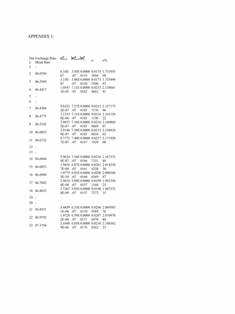
Date

Exchange Rate-Mean Rate

σ σ%

1 -

2 86.0769 6.16E-07

3.95E-07

0.00000119

0.01733956

1.73395590

3 86.3569 3.15E-07

3.96E-07

0.00000120

0.01735500

1.73549983

4 86.4417 1.05471E-05

7.11E-07

0.00000182

0.02138662

2.13866191

5 -

6 -

7 86.4264 9.63322E-07

7.27E-07

0.00000185

0.02157176

2.15717596

8 86.4775 3.13338E-08

7.31E-07

0.00000185

0.02161130

2.16113022

9 86.5242 3.49375E-07

7.30E-07

0.00000185

0.02160869

2.16086907

10 86.6053 2.91469E-07

7.29E-07

0.00000185

0.02158834

2.15883403

11 86.6722 8.77727E-07

7.40E-07

0.00000187

0.02171929

2.17192908

12 -

13 -

14 86.6844 5.96249E-07

7.36E-07

0.00000186

0.02167331

2.16733148

15 86.6853 1.98107E-08

6.07E-07

0.00000161

0.02014238

2.01423830

16 86.6989 1.07795E-10

6.01E-07

0.00000160

0.02006569

2.00656887

17 86.7042 2.46104E-08

5.89E-07

0.00000157

0.01991544

1.99154423

18 86.8653 3.73678E-09

5.85E-07

0.00000157

0.01987272

1.98727215

19 -

20 -

21 86.8531 3.44591E-06

6.53E-07

0.00000170

0.02069584

2.06958378

22 86.9792 1.97282E-08

6.59E-07

0.00000171

0.02076970

2.07697040

23 87.3794 2.10489E-06

6.85E-07

0.00000176

0.02108362

2.10836233

APPENDIX 1:

APPENDIX 2

:

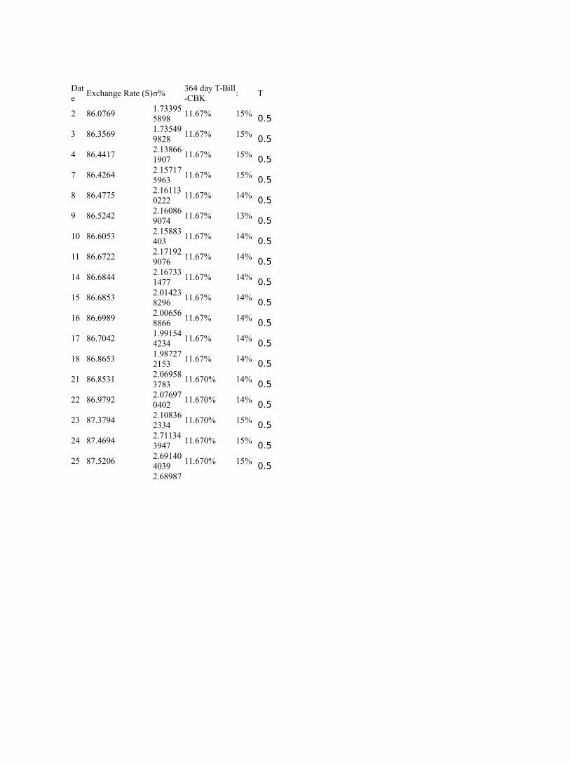
Date

Exchange Rate (S)σ% 364 day T-Bill-CBK

: T

2 86.0769 1.733955898

11.67% 15% 0.5

3 86.3569 1.735499828

11.67% 15% 0.5

4 86.4417 2.138661907

11.67% 15% 0.5

7 86.4264 2.157175963

11.67% 15% 0.5

8 86.4775 2.161130222

11.67% 14% 0.5

9 86.5242 2.160869074

11.67% 13% 0.5

10 86.6053 2.15883403

11.67% 14% 0.5

11 86.6722 2.171929076

11.67% 14% 0.5

14 86.6844 2.167331477

11.67% 14% 0.5

15 86.6853 2.014238296

11.67% 14% 0.5

16 86.6989 2.006568866

11.67% 14% 0.5

17 86.7042 1.991544234

11.67% 14% 0.5

18 86.8653 1.987272153

11.67% 14% 0.5

21 86.8531 2.069583783

11.670% 14% 0.5

22 86.9792 2.076970402

11.670% 14% 0.5

23 87.3794 2.108362334

11.670% 15% 0.5

24 87.4694 2.711343947

11.670% 15% 0.5

25 87.5206 2.691404039

11.670% 15% 0.5 2.68987

APPENDIX 3: Daily Mean Exchange Rates (January 2008-December 2012)

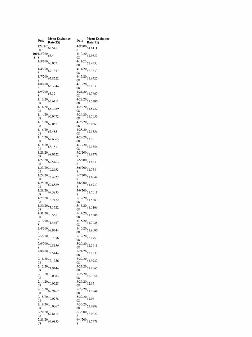
Date Mean ExchangeRate(Et)

Date Mean ExchangeRate(Et)

12/31/2007

62.5411 4/9/2008

64.6111

2008

1/2/2008

63.4 4/10/2008

62.9833

1/3/2008

65.0571 4/11/2008

62.4333

1/4/2008

67.1357 4/14/2008

62.3633

1/7/2008

65.8222 4/15/2008

61.6722

1/8/2008

65.3944 4/18/2008

62.1633

1/9/2008

65.32 4/21/2008

61.7667

1/10/2008

65.6111 4/22/2008

61.5206

1/11/2008

65.3389 4/23/2008

61.5722

1/14/2008

66.0472 4/24/2008

61.7056

1/15/2008

67.0611 4/25/2008

62.0667

1/16/2008

67.485 4/28/2008

62.1556

1/17/2008

67.6063 4/29/2008

62.25

1/18/2008

68.1511 4/30/2008

62.1356

1/21/2008

68.9222 5/2/2008

61.9778

1/22/2008

69.5163 5/5/2008

61.8333

1/23/2008

70.2933 5/6/2008

61.7544

1/24/2008

73.4722 5/7/2008

61.6044

1/25/2008

69.8889 5/8/2008

61.6733

1/28/2008

69.5833 5/9/2008

61.7011

1/29/2008

72.7472 5/12/2008

61.5883

1/30/2008

73.3722 5/13/2008

61.5106

1/31/2008

70.5611 5/14/2008

61.5306

2/1/2008

71.4667 5/15/2008

61.7028

2/4/2008

69.9744 5/16/2008

61.9006

2/5/2008

70.7056 5/19/2008

62.175

2/6/2008

70.8156 5/20/2008

62.3611

2/8/2008

72.5444 5/21/2008

62.1533

2/11/2008

72.1756 5/22/2008

61.9722

2/12/2008

71.9144 5/23/2008

61.9067

2/13/2008

70.0083 5/26/2008

62.3056

2/14/2008

70.0528 5/27/2008

62.15

2/15/2008

69.9167 5/28/2008

61.9944

2/18/2008

70.0278 5/29/2008

62.06

2/19/2008

70.0367 5/30/2008

62.0289

2/20/2008

69.8111 6/3/2008

62.0222

2/21/2008

69.6833 6/4/2008

61.7978

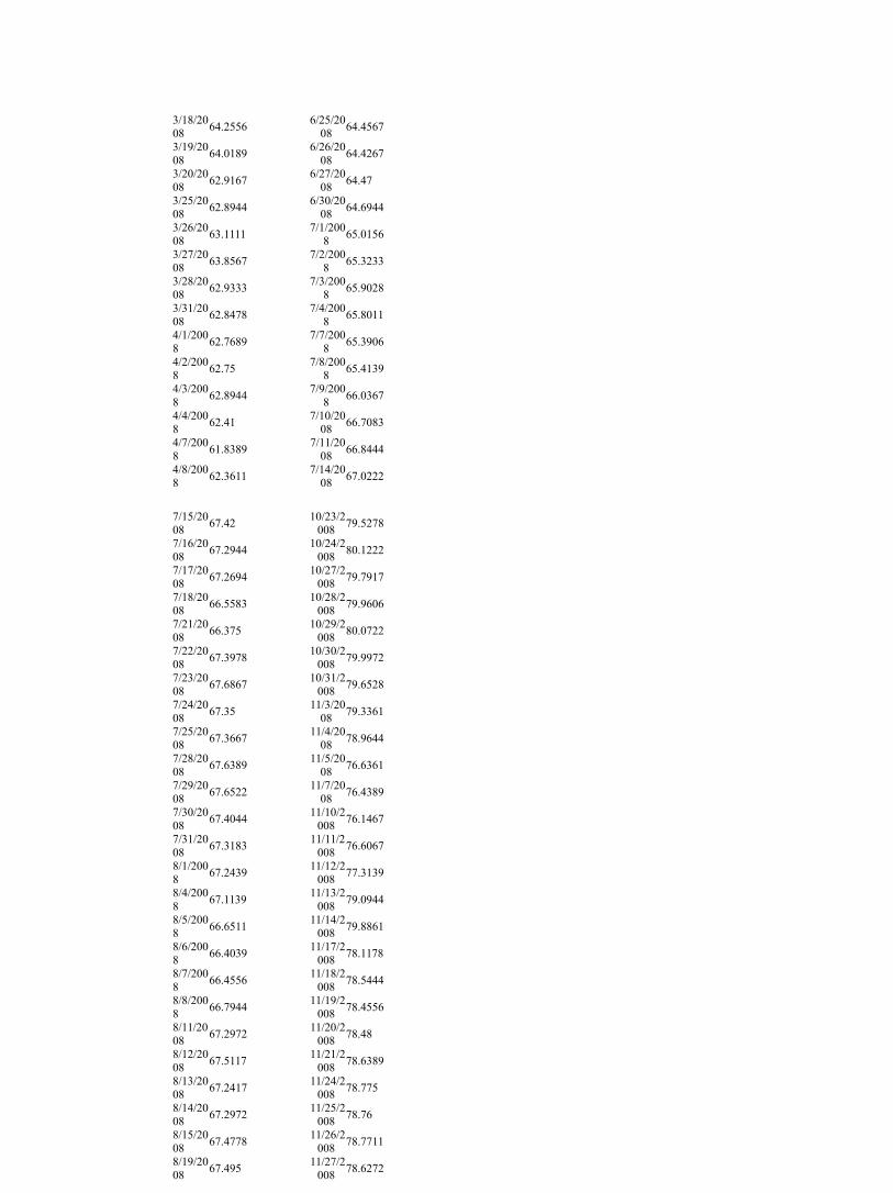
3/18/2008

64.2556 6/25/20

08 64.4567

3/19/2008

64.0189 6/26/20

08 64.4267

3/20/2008

62.9167 6/27/20

08 64.47

3/25/2008

62.8944 6/30/20

08 64.6944

3/26/2008

63.1111 7/1/200

8 65.0156

3/27/2008

63.8567 7/2/200

8 65.3233

3/28/2008

62.9333 7/3/200

8 65.9028

3/31/2008

62.8478 7/4/200

8 65.8011

4/1/2008

62.7689 7/7/200

8 65.3906

4/2/2008

62.75 7/8/200

8 65.4139

4/3/2008

62.8944 7/9/200

8 66.0367

4/4/2008

62.41 7/10/20

08 66.7083

4/7/2008

61.8389 7/11/20

08 66.8444

4/8/2008

62.3611 7/14/20

08 67.0222

7/15/2008

67.42 10/23/2

008 79.5278

7/16/2008

67.2944 10/24/2

008 80.1222

7/17/2008

67.2694 10/27/2

008 79.7917

7/18/2008

66.5583 10/28/2

008 79.9606

7/21/2008

66.375 10/29/2

008 80.0722

7/22/2008

67.3978 10/30/2

008 79.9972

7/23/2008

67.6867 10/31/2

008 79.6528

7/24/2008

67.35 11/3/20

08 79.3361

7/25/2008

67.3667 11/4/20

08 78.9644

7/28/2008

67.6389 11/5/20

08 76.6361

7/29/2008

67.6522 11/7/20

08 76.4389

7/30/2008

67.4044 11/10/2

008 76.1467

7/31/2008

67.3183 11/11/2

008 76.6067

8/1/2008

67.2439 11/12/2

008 77.3139

8/4/2008

67.1139 11/13/2

008 79.0944

8/5/2008

66.6511 11/14/2

008 79.8861

8/6/2008

66.4039 11/17/2

008 78.1178

8/7/2008

66.4556 11/18/2

008 78.5444

8/8/2008

66.7944 11/19/2

008 78.4556

8/11/2008

67.2972 11/20/2

008 78.48

8/12/2008

67.5117 11/21/2

008 78.6389

8/13/2008

67.2417 11/24/2

008 78.775

8/14/2008

67.2972 11/25/2

008 78.76

8/15/2008

67.4778 11/26/2

008 78.7711

8/19/2008

67.495 11/27/2

008 78.6272

9/9/2008

70.2583 12/19/2008

76.3067

9/10/2008

70.4056 12/22/2008

75.6411

9/11/2008

70.6222 12/23/2008

76.8778

9/12/2008

70.7067 12/24/2008

77.0778

9/15/2008

70.5311 12/29/2008

76.8389

9/16/2008

70.7417 12/30/2008

77.6833

9/17/2008

71.8639 12/31/2008

77.7111

9/18/2008

72.8417 2009

1/2/2009

78.2678

9/19/2008

72.9761 1/5/2009

78.8389

9/22/2008

71.9306 1/6/2009

79.2822

9/23/2008

72.8044 1/7/2009

78.7167

9/24/2008

73.1022 1/8/2009

78.2317

9/26/2008

73.8778 1/9/2009

77.4361

9/29/2008

73.8267 1/12/2009

77.665

9/30/2008

73.2189 1/13/2009

77.8944

10/2/2008

73.1728 1/14/2009

78.6306

10/3/2008

72.9678 1/15/2009

78.8306

10/6/2008

72.9117 1/16/2009

79.7567

10/7/2008

73.6728 1/19/2009

78.7417

10/8/2008

73.7656 1/20/2009

78.9539

10/9/2008

74.1772 1/21/2009

79.7028

10/13/2008

74.3333 1/22/2009

80.0083

10/14/2008

75.9722 1/23/2009

79.7339

10/15/2008

75.5861 1/26/2009

79.7167

10/16/2008

75.5894 1/27/2009

79.6139

10/17/2008

77.2917 1/28/2009

79.7961

10/21/2008

76.3944 1/29/2009

79.6317

10/22/2008

78.1833 1/30/2009

79.5439

2/2/2009

79.6461 5/11/2009

77.8833

2/3/2009

79.4583 5/12/2009

77.4778

2/4/2009

79.4789 5/13/2009

76.9361

2/5/2009

79.4 5/14/2009

77.0522

2/6/2009

79.3172 5/15/2009

78.3278

2/9/2009

79.3983 5/18/2009

78.2139

2/10/2009

79.2478 5/19/2009

78.3383

2/11/2009

79.1028 5/20/2009

78.0972

2/12/2009

79.05 5/21/2009

77.7894

2/13/2009

79.6528 5/22/2009

77.975

2/16/2009

79.55 5/25/2009

77.8756

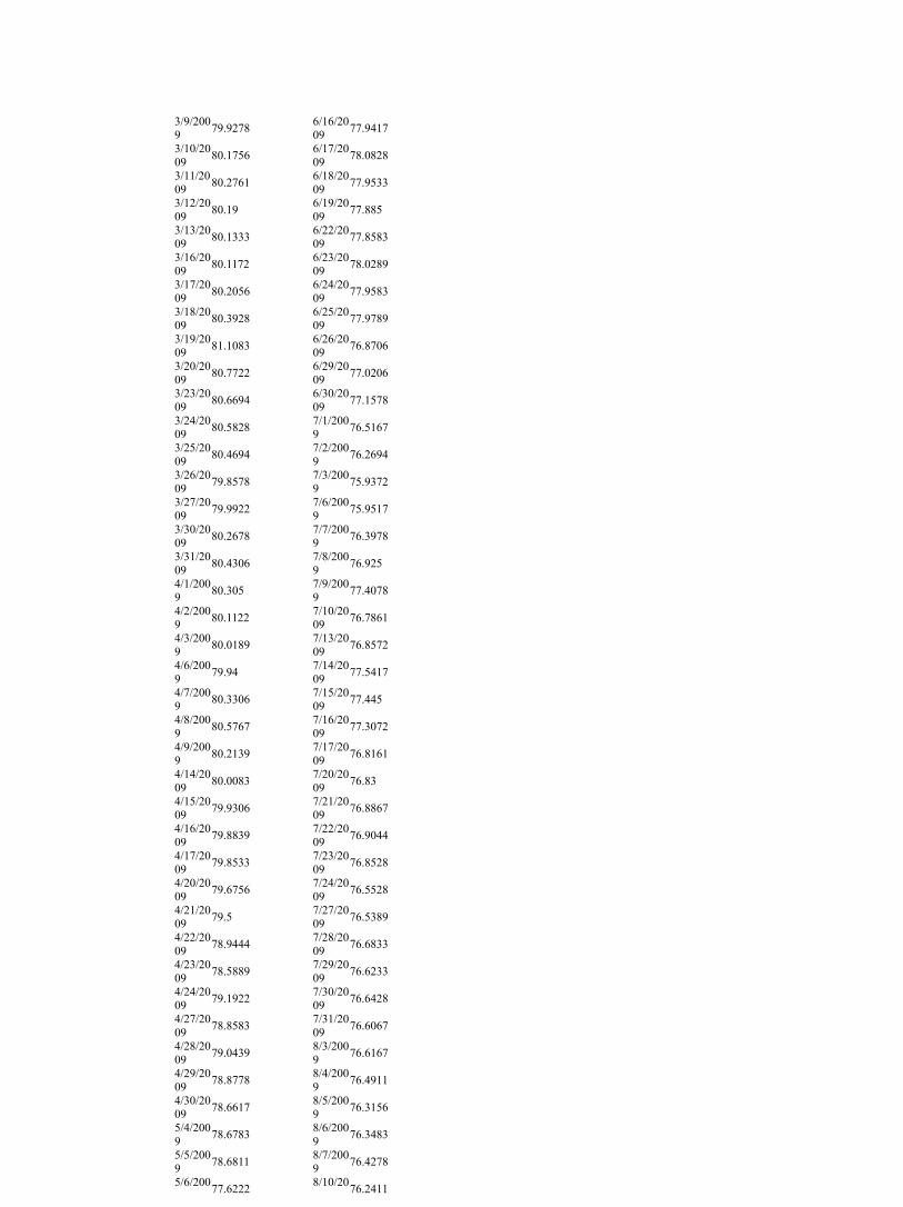
3/9/2009

79.9278 6/16/2009

77.9417

3/10/2009

80.1756 6/17/2009

78.0828

3/11/2009

80.2761 6/18/2009

77.9533

3/12/2009

80.19 6/19/2009

77.885

3/13/2009

80.1333 6/22/2009

77.8583

3/16/2009

80.1172 6/23/2009

78.0289

3/17/2009

80.2056 6/24/2009

77.9583

3/18/2009

80.3928 6/25/2009

77.9789

3/19/2009

81.1083 6/26/2009

76.8706

3/20/2009

80.7722 6/29/2009

77.0206

3/23/2009

80.6694 6/30/2009

77.1578

3/24/2009

80.5828 7/1/2009

76.5167

3/25/2009

80.4694 7/2/2009

76.2694

3/26/2009

79.8578 7/3/2009

75.9372

3/27/2009

79.9922 7/6/2009

75.9517

3/30/2009

80.2678 7/7/2009

76.3978

3/31/2009

80.4306 7/8/2009

76.925

4/1/2009

80.305 7/9/2009

77.4078

4/2/2009

80.1122 7/10/2009

76.7861

4/3/2009

80.0189 7/13/2009

76.8572

4/6/2009

79.94 7/14/2009

77.5417

4/7/2009

80.3306 7/15/2009

77.445

4/8/2009

80.5767 7/16/2009

77.3072

4/9/2009

80.2139 7/17/2009

76.8161

4/14/2009

80.0083 7/20/2009

76.83

4/15/2009

79.9306 7/21/2009

76.8867

4/16/2009

79.8839 7/22/2009

76.9044

4/17/2009

79.8533 7/23/2009

76.8528

4/20/2009

79.6756 7/24/2009

76.5528

4/21/2009

79.5 7/27/2009

76.5389

4/22/2009

78.9444 7/28/2009

76.6833

4/23/2009

78.5889 7/29/2009

76.6233

4/24/2009

79.1922 7/30/2009

76.6428

4/27/2009

78.8583 7/31/2009

76.6067

4/28/2009

79.0439 8/3/2009

76.6167

4/29/2009

78.8778 8/4/2009

76.4911

4/30/2009

78.6617 8/5/2009

76.3156

5/4/2009

78.6783 8/6/2009

76.3483

5/5/2009

78.6811 8/7/2009

76.4278

5/6/20077.6222

8/10/2076.2411

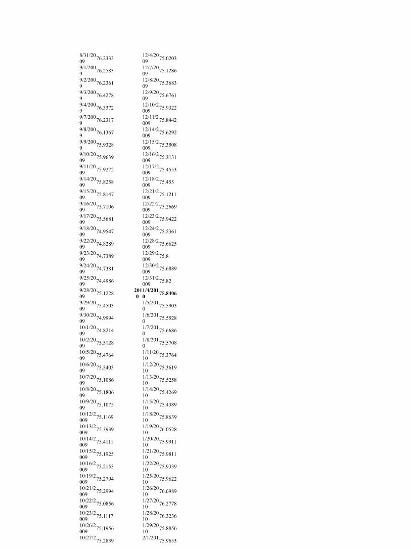
8/31/2009

76.2333 12/4/2009

75.0203

9/1/2009

76.2583 12/7/2009

75.1286

9/2/2009

76.2361 12/8/2009

75.3683

9/3/2009

76.4278 12/9/2009

75.6761

9/4/2009

76.3372 12/10/2009

75.9322

9/7/2009

76.2317 12/11/2009

75.8442

9/8/2009

76.1367 12/14/2009

75.6292

9/9/2009

75.9328 12/15/2009

75.3508

9/10/2009

75.9639 12/16/2009

75.3131

9/11/2009

75.9272 12/17/2009

75.4553

9/14/2009

75.8258 12/18/2009

75.455

9/15/2009

75.8147 12/21/2009

75.1211

9/16/2009

75.7106 12/22/2009

75.2669

9/17/2009

75.5681 12/23/2009

75.9422

9/18/2009

74.9547 12/24/2009

75.5361

9/22/2009

74.8289 12/28/2009

75.6625

9/23/2009

74.7389 12/29/2009

75.8

9/24/2009

74.7381 12/30/2009

75.6889

9/25/2009

74.4986 12/31/2009

75.82

9/28/2009

75.1228 2010

1/4/2010

75.8406

9/29/2009

75.4503 1/5/2010

75.5903

9/30/2009

74.9994 1/6/2010

75.5528

10/1/2009

74.8214 1/7/2010

75.6686

10/2/2009

75.5128 1/8/2010

75.5708

10/5/2009

75.4764 1/11/2010

75.3764

10/6/2009

75.5403 1/12/2010

75.3619

10/7/2009

75.1086 1/13/2010

75.5258

10/8/2009

75.1806 1/14/2010

75.4269

10/9/2009

75.1075 1/15/2010

75.4389

10/12/2009

75.1169 1/18/2010

75.8639

10/13/2009

75.3939 1/19/2010

76.0528

10/14/2009

75.4111 1/20/2010

75.9911

10/15/2009

75.1925 1/21/2010

75.9811

10/16/2009

75.2153 1/22/2010

75.9339

10/19/2009

75.2794 1/25/2010

75.9622

10/21/2009

75.2994 1/26/2010

76.0989

10/22/2009

75.0856 1/27/2010

76.2778

10/23/2009

75.1117 1/28/2010

76.3236

10/26/2009

75.1956 1/29/2010

75.8856

10/27/275.2839

2/1/20175.9653

11/17/2009

74.7161 2/22/2010

76.7814

11/18/2009

74.4722 2/23/2010

76.8386

2/24/2010

76.9681 6/2/2010

79.8929

2/25/2010

77.0556 6/3/2010

80.0085

2/26/2010

76.8972 6/4/2010

80.2228

3/1/2010

76.8083 6/7/2010

81.5586

3/2/2010

76.9378 6/8/2010

82.1028

3/3/2010

76.8931 6/9/2010

81.9486

3/4/2010

76.8486 6/10/2010

81.7458

3/5/2010

76.7447 6/11/2010

80.6889

3/8/2010

76.7944 6/14/2010

80.6806

3/9/2010

76.6653 6/15/2010

80.6958

3/10/2010

76.7778 6/16/2010

80.55

3/11/2010

76.6608 6/17/2010

80.7194

3/12/2010

76.7197 6/18/2010

80.7117

3/15/2010

76.6639 6/21/2010

80.5264

3/16/2010

76.8444 6/22/2010

80.6361

3/17/2010

76.8292 6/23/2010

80.9936

3/18/2010

76.8569 6/24/2010

80.9375

3/19/2010

76.9714 6/25/2010

81.6153

3/22/2010

76.9539 6/28/2010

81.4694

3/23/2010

77.0489 6/29/2010

81.7583

3/24/2010

77.0531 6/30/2010

81.9167

3/25/2010

77.4586 7/1/2010

81.7958

3/26/2010

77.3089 7/2/2010

81.6583

3/29/2010

77.3017 7/5/2010

81.4225

3/30/2010

77.3025 7/6/2010

81.4919

3/31/2010

77.3314 7/7/2010

81.5422

4/1/2010

77.2975 7/8/2010

81.4847

4/6/2010

77.2083 7/9/2010

81.4475

4/7/2010

77.2097 7/12/2010

81.5097

4/8/2010

77.2994 7/13/2010

81.8106

4/9/2010

77.2767 7/14/2010

81.6839

4/12/2010

77.1708 7/15/2010

81.6033

4/13/2010

77.175 7/16/2010

81.4375

4/14/2010

77.0978 7/19/2010

81.5417

4/15/2010

76.9472 7/20/2010

81.5861

4/16/2010

77.0281 7/21/2010

81.8403

4/19/2010

77.3481 7/22/2010

81.8153

5/10/2010

77.9713 8/13/2010

80.3983

5/11/2010

77.8241 8/16/2010

80.4208

5/12/2010

77.8899 8/17/2010

80.4872

5/13/2010

77.8009 8/18/2010

80.5286

5/14/2010

78.0468 8/19/2010

80.7806

5/17/2010

78.3497 8/20/2010

81.0153

5/18/2010

78.6397 8/23/2010

81.085

5/19/2010

78.7834 8/24/2010

81.3628

5/20/2010

79.1712 8/25/2010

81.2428

5/21/2010

79.4427 8/26/2010

80.7819

5/24/2010

79.2471 8/30/2010

80.8731

5/25/2010

79.5467 8/31/2010

81.0711

5/26/2010

79.7868 9/1/2010

80.9742

5/27/2010

79.7463 9/2/2010

80.7689

5/28/2010

79.7171 9/3/2010

80.7272

5/31/2010

79.7453 9/6/2010

80.6708

9/7/2010

80.9442 12/10/2010

80.5578

9/8/2010

81.1514 12/14/2010

80.5153

9/9/2010

81.2619 12/15/2010

80.5239

9/10/2010

81.2703 12/16/2010

80.6325

9/13/2010

80.8933 12/17/2010

80.5375

9/14/2010

80.9303 12/20/2010

80.5308

9/15/2010

80.8592 12/21/2010

80.4886

9/16/2010

80.8403 12/22/2010

80.4906

9/17/2010

80.5903 12/23/2010

80.5733

9/20/2010

80.7869 12/24/2010

80.5903

9/21/2010

80.9917 12/27/2010

80.6625

9/22/2010

80.8358 12/28/2010

80.6144

9/23/2010

80.9486 12/29/2010

80.6292

9/24/2010

81.1597 12/30/2010

80.6714

9/27/2010

80.8917 12/31/2010

80.7519

9/28/2010

80.9375 2011

1/3/2011

80.7961

9/29/2010

80.8503 1/4/2011

80.995

9/30/2010

80.7781 1/5/2011

80.9389

10/1/2010

80.8444 1/6/2011

81.1322

10/4/2010

80.8361 1/7/2011

81.1444

10/5/2010

80.8411 1/10/2011

81.1747

10/6/2010

80.7172 1/11/2011

81.2181

10/7/2010

80.63 1/12/2011

81.0708

10/29/2010

80.7869 2/2/2011

81.1014

11/1/2010

80.7539 2/3/2011

81.0667

11/2/2010

80.7394 2/4/2011

81.1889

11/3/2010

80.5586 2/7/2011

81.1472

11/4/2010

80.5308 2/8/2011

81.2042

11/5/2010

80.1356 2/9/2011

81.2167

11/8/2010

80.3333 2/10/2011

81.2375

11/9/2010

80.6236 2/11/2011

81.3014

11/10/2010

80.6344 2/14/2011

81.4428

11/11/2010

80.5469 2/15/2011

81.3869

11/12/2010

80.5986 2/16/2011

81.3583

11/15/2010

80.5147 2/17/2011

81.3942

11/16/2010

80.4572 2/18/2011

81.4456

11/17/2010

80.45 2/21/2011

81.7936

11/18/2010

80.1639 2/22/2011

81.8611

11/19/2010

80.1006 2/23/2011

81.875

11/22/2010

80.0397 2/24/2011

81.8917

11/23/2010

80.1625 2/25/2011

81.9992

11/24/2010

80.3486 2/28/2011

82.3639

11/25/2010

80.2931 3/1/2011

82.6014

11/26/2010

80.3892 3/2/2011

82.8031

11/29/2010

80.7764 3/3/2011

82.9278

11/30/2010

80.9742 3/4/2011

83.0542

12/1/2010

80.8972 3/7/2011

83.0081

12/2/2010

80.3208 3/8/2011

83.0833

12/3/2010

80.4625 3/9/2011

83.4667

12/6/2010

80.4364 3/10/2011

84.0447

12/7/2010

80.4831 3/11/2011

84.6569

12/8/2010

80.5525 3/14/2011

84.9294

12/9/2010 80.5736

3/15/2011 86.3239

3/16/2011

85.8572 6/23/2011

90.5597

3/17/2011

85.8108 6/24/2011

90.4486

3/18/2011

85.0417 6/27/2011

90.4625

3/21/2011

84.5917 6/28/2011

90.8278

3/22/2011

85.1486 6/29/2011

90.0236

3/23/2011

84.7847 6/30/2011

89.8639

3/24/2011

84.9931 7/1/2011

89.3597

3/25/2011

84.9444 7/4/2011

88.6856

3/28/2011

84.2944 7/5/2011

88.4514

4/18/2011

84.0056 7/26/2011

90.375

4/19/2011

83.8417 7/27/2011

90.5111

4/20/2011

83.9181 7/28/2011

90.8444

4/21/2011

83.9828 7/29/2011

91.1

4/26/2011

83.9278 8/1/2011

90.975

4/27/2011

83.5708 8/2/2011

91.2111

4/28/2011

83.625 8/3/2011

91.5847

4/29/2011

83.4194 8/4/2011

91.9361

5/3/2011

83.4583 8/5/2011

92.3528

5/4/2011

83.5278 8/8/2011

92.7667

5/5/2011

83.6556 8/9/2011

93.7375

5/6/2011

84.05 8/10/2011

94.5167

5/9/2011

84.2208 8/11/2011

93.9131

5/10/2011

84.7056 8/12/2011

93.2328

5/11/2011

85.2222 8/15/2011

92.7183

5/12/2011

85.9244 8/16/2011

92.85

5/13/2011

86.1139 8/17/2011

93.1431

5/16/2011

85.9333 8/18/2011

93.1361

5/17/2011

86.2514 8/19/2011

92.9028

5/18/2011

86.5611 8/22/2011

93.0097

5/19/2011

87.0486 8/23/2011

92.8056

5/20/2011

86.0261 8/24/2011

92.7306

5/23/2011

86.1528 8/25/2011

92.4042

5/24/2011

86.1472 8/26/2011

92.8931

5/25/2011

86.4208 8/29/2011

92.8489

5/26/2011

86.0111 8/30/2011

93.6222

5/27/2011

85.4417 9/1/2011

93.6806

5/30/2011

85.5161 9/2/2011

94.1097

5/31/2011

85.7044 9/5/2011

94.4278

6/2/2011

86.375 9/6/2011

94.7722

6/3/2011

86.7514 9/7/2011

93.4597

6/6/2011

86.8292 9/8/2011

93.9903

6/7/2011

87.0422 9/9/2011

93.7083

6/8/2011

87.7219 9/12/2011

94.1111

6/9/2011

87.5569 9/13/2011

95.4306

6/10/2011

87.6625 9/14/2011

94.7819

6/13/2011

88.0931 9/15/2011

94.9708

6/14/2011

89.3708 9/16/2011

94.8056

6/15/2011

89.2361 9/19/2011

95.1928

6/16/2088.9764

9/20/2095.8361

10/10/2011

102.811 1/17/2012

86.9583

10/11/2011

103.908 1/18/2012

86.3331

10/12/2011

105.961 1/19/2012

86.2197

10/13/2011

104.01 1/20/2012

85.6778

10/14/2011

101.426 1/23/2012

86.0444

10/17/2011

100.512 1/24/2012

86.1

10/18/2011

99.1861 1/25/2012

85.8444

10/19/2011

99.5181 1/26/2012

85.3639

10/21/2011

99.7014 1/27/2012

85.0306

10/24/2011

100.117 1/30/2012

84.9167

10/25/2011

100.596 1/31/2012

84.5875

10/26/2011

101.443 2/1/2012

83.8833

10/27/2011

100.632 2/2/2012

83.5861

10/28/2011

99.0319 2/3/2012

83.8708

10/31/2011

99.7783 2/6/2012

83.8125

11/1/2011

99.3347 2/7/2012

83.4903

11/2/2011

96.5222 2/8/2012

83.1403

11/3/2011

96.8097 2/9/2012

82.7167

11/4/2011

96.975 2/10/2012

83.9278

11/7/2011

97.3819 2/13/2012

82.8125

11/8/2011

96.9706 2/14/2012

82.9583

11/9/2011

96.2694 2/15/2012

82.93

11/10/2011

95.6903 2/16/2012

83.1667

11/11/2011

94.7989 2/17/2012

83.0722

11/14/2011

93.2164 2/20/2012

82.9097

11/15/2011

93.7208 2/21/2012

83.2972

11/16/2011

94.1458 2/22/2012

83.2944

11/17/2011

93.6806 2/23/2012

82.7569

11/18/2011

92.5433 2/24/2012

82.6986

11/21/2011

91.0417 2/27/2012

82.6519

11/22/2011

90.6722 2/28/2012

82.7514

11/23/2011

90.0611 2/29/2012

82.9708

11/24/2011

90.3097 3/1/2012

83.2625

11/25/2011

90.2681 3/2/2012

83.2561

11/28/2011

90.5611 3/5/2012

83.2347

11/29/2011

90.1681 3/6/2012

83.3625

11/30/2011

89.7208 3/7/2012

82.8222

12/1/2011

89.5972 3/8/2012

82.8292

12/2/2011

89.7125 3/9/2012

82.7514

12/5/2089.8281

3/9/20184.1483

12/28/2011

83.7167 3/29/2012

83.0153

12/29/2011

84.6667 3/30/2012

83.0556

12/30/2011

85.0681 4/2/2012

83.1014

2012

1/3/2012 85.0906

4/3/2012

83.0694

4/4/2012

83.1764 7/12/2012

83.9292

4/5/2012

83.0667 7/13/2012

84.0265

4/10/2012

83.1031 7/16/2012

84.1222

4/11/2012

83.1961 7/17/2012

84.1889

4/12/2012

83.2541 7/18/2012

84.1794

4/13/2012

83.3681 7/19/2012

84.1558

4/16/2012

83.1611 7/20/2012

84.1447

4/17/2012

83.15 7/23/2012

84.1917

4/18/2012

83.1389 7/24/2012

84.2617

4/19/2012

83.1542 7/25/2012

84.2997

4/20/2012

83.1969 7/26/2012

84.2292

4/23/2012

83.2178 7/27/2012

84.2011

4/24/2012

83.2293 7/30/2012

84.2014

4/25/2012

83.2531 7/31/2012

84.2125

4/26/2012

83.265 8/1/2012

84.2383

4/27/2012

83.25 8/2/2012

84.2264

4/30/2012

83.2164 8/3/2012

84.2506

5/2/2012

83.2903 8/6/2012

84.2022

5/3/2012

83.4053 8/7/2012

84.095

5/4/2012

83.2806 8/8/2012

83.9367

5/7/2012

83.2703 8/9/2012

84.0875

5/8/2012

83.2831 8/10/2012

84.0139

5/9/2012

83.2958 8/13/2012

84.0506

5/10/2012

83.3972 8/14/2012

83.8975

5/11/2012

83.6181 8/15/2012

83.9333

5/14/2012

83.6764 8/16/2012

83.9833

5/15/2012

83.9469 8/17/2012

84.0672

5/16/2012

84.9572 8/21/2012

83.975

5/17/2012

84.5639 8/22/2012

84.0056

5/18/2012

85.1625 8/23/2012

83.9903

5/21/2012

84.9572 8/24/2012

84.0056

5/22/2012

84.5639 8/27/2012

84.0236

5/23/2012

85.1625 8/28/2012

84.0961

5/24/2012

85.2558 8/29/2012

84.1181

5/25/2012

85.3153 8/30/2012

84.1422

6/18/2012

84.8847 9/20/2012

84.8275

6/19/2012

84.525 9/21/2012

84.8264

6/20/2012

84.1556 9/24/2012

84.8667

6/21/2012

83.6403 9/25/2012

84.8444

6/22/2012

84.0125 9/26/2012

85.0097

6/25/2012

83.9472 9/27/2012

85.1764

6/26/2012

84.2519 9/28/2012

85.2833

6/27/2012

84.1625 10/1/2012

85.2764

6/28/2012

84.1478 10/2/2012

85.1764

6/29/2012

84.2333 10/3/2012

84.9714

7/2/2012

84.1322 10/4/2012

84.925

7/3/2012

84.1231 10/5/2012

84.9125

7/4/2012

84.0278 10/8/2012

84.9153

7/5/2012

84.0347 10/9/2012

85.1019

7/6/2012

84.5292 10/10/2012

85.0978

7/9/2012

84.0972 10/11/2012

85.1175

7/10/2012

83.9368 10/12/2012

85.1339

7/11/2012 83.9588

10/15/2012 85.1383

10/16/2012 85.1261

10/17/2012

85.0342

10/18/2012

85.0422

10/19/2012

85.1667

10/22/2012

85.1819

10/23/2012

85.2328

10/24/2012

85.2208

10/25/2012

85.1472

10/26/2012

85.1342

10/29/2012

85.1692

10/30/2012

85.1678

10/31/2012

85.1775

11/1/2012

85.2361

11/2/2012

85.3083

11/5/2012

85.4456

11/6/2012

85.55

11/7/2012

85.5069

11/8/2012

85.41

11/9/2012

85.3778

11/12/2012

85.3994

11/13/2012

85.5283

11/14/2

12/4/2012

85.9639

12/5/2012

85.9417

12/6/2012

85.9889

12/7/2012

85.9575

12/10/2012

85.9889

12/11/2012

86.0522

12/13/2012

86.0422

12/14/2012

86.0383

12/17/2012

86.0672

12/18/2012

86.0611

12/19/2012

86.0744

12/20/2012

86.0472

12/21/2012

86.0008

12/24/2012

85.9039

12/27/2012

85.8628

12/28/2012

85.9611

12/31/2012

86.0286