THE VALUATION OF CORRELATION-DEPENDENT CREDIT DERIVATIVES USING A

STRUCTURAL MODEL

John Hull, Mirela Predescu, and Alan White*

First Draft: March 2005

This Draft: November 2006

*John Hull and Alan White are at the Joseph L. Rotman School of Management, University of Toronto, Canada. Mirela Predescu is at the Saïd Business School, Oxford University, UK. We are grateful to Moody’s Investment Services for providing financial support for this research and to GFI for providing data. We are also grateful for helpful discussions with Leif Andersen, Darrell Duffie, Jon Gregory, Marek Musiela and for the comments of seminar participants at the INI Credit Workshop at Cambridge University’s Isaac Newton Institute, the Moody’s/London Business School Second Annual Credit Risk Conference, the 2005 meeting of the Northern Finance Association, and the Credit Risk Workshop at the Statistical and Applied Mathematical Sciences Institute.

2

The Valuation of Correlation-Dependent Credit Derivatives Using a Structural Model

John Hull, Mirela Predescu, and Alan White

ABSTRACT

In 1976 Black and Cox proposed a structural model where an obligor defaults when the value of its assets

hits a certain barrier. In 2001 Zhou showed how the model can be extended to two obligors whose assets

are correlated. In this paper we show how the model can be extended to a large number of different

obligors. The correlations between the assets of the obligors are determined by one or more factors. We

examine the dynamics of credit spreads implied by the model and explore how the model prices tranches

of collateralized debt obligations (CDOs). We compare the model with the widely used Gaussian copula

model of survival time and test how well the model fits market data on the prices of CDO tranches. We

consider three extensions of the model. The first reflects empirical research showing that default

correlations are positively dependent on default rates. The second reflects empirical research showing that

recovery rates are negatively dependent on default rates. The third reflects research showing that market

prices are consistent with heavy tails for both the common factor and the idiosyncratic factor in a copula

model.

3

The Valuation of Correlation-Dependent Credit Derivatives Using a Structural Model

The trading of products whose values depend on credit correlation has grown rapidly in recent years. The

most popular credit-correlation product is a collateralized debt obligation (CDO). The size of the market

for CDOs in 2005, measured in terms of notional principal of outstanding transactions, is estimated to be

$2 trillion. This compares with a total market for all credit derivatives of about $12 trillion.

A CDO is a structure that distributes credit risk to investors in much the same way that collateralized

mortgage obligations distribute prepayment risk. The early CDOs were known as cash CDOs. The

arranger of the CDO would buy a portfolio of bonds and distribute the credit risk to investors by creating

tranches. The first tranche would be responsible for all credit losses between 0% and K1% of the total

principal; the second tranche would be responsible for all credit losses between K1% and K2% of the total

principal; and so on. The market then moved to creating what are known as synthetic CDOs where the

arranger of the CDO sells a portfolio of credit default swaps in the market and then distributes the credit

risk to investors by creating tranches in the same way as for a cash CDO. A third development in the

CDO market involves what is known as “single tranche trading”. A portfolio and a tranche are defined

and the buyer and seller of protection agree to exchange the cash flows that would have been applicable if

a synthetic CDO had been set up.

The growth of single tranche trading has been helped by the establishment of standard portfolios. The

most important standard portfolios are CDX IG, a portfolio of 125 investment grade companies in the

United States, and iTraxx IG, a portfolio of 125 European investment grade companies. Standard credit-

loss tranches for these portfolios have been defined and bid and ask quotes for the CDX and iTraxx

tranches are now available through Reuters.

To value a CDO tranche it is necessary to develop a model of the joint probability of default of the

companies in the underlying portfolio. The first structural model of default for a single company was

produced by Merton (1974). In this model a default occurs if the value of the assets of the company is

below the face value of the debt at a particular future time. Black and Cox (1976) provide an important

extension of Merton’s model. Their model has a first passage time structure where a default takes place

whenever the value of the assets of a company drops below a barrier level. Other extensions of the

Merton’s model are provided by Geske (1977), Kim, Ramaswamy and Sundaresan (1993), Leland (1994),

4

Longstaff and Schwartz (1995), Leland and Toft (1996), and Zhou (2001a). All these papers looked at

the default probability of only one issuer.

Zhou (2001b) and Hull and White (2001) were the first to incorporate default correlation between

different issuers into the Black and Cox first passage time structural model. Zhou (2001b) finds a closed-

form formula for the joint default probability of two issuers, but his results cannot easily be extended to

more than two issuers. Hull and White (2001) show how many issuers can be handled, but their

correlation model requires computationally time-consuming numerical procedures.

In this paper we provide a way to model default correlation using the Black-Cox structural model

framework. Our approach can be used to price and calculate deltas for credit derivatives and is

computationally feasible when there are a large number of different companies. We assume that the

correlation between the asset values of different companies is driven by one or more common factors. We

consider, first, a base case model, where the asset correlation and the recovery rate are both constant. We

then extend the base case model in three ways. The first allows the asset correlation to be stochastic and

correlated with default rates. This is motivated by empirical evidence that suggests that asset correlations

are stochastic and increase when default rates are high (see Servigny and Renault (2002), Das, Freed,

Geng and Kapadia (2004) and Ang and Chen (2002)). The second assumes that the recovery rate is

stochastic and correlated with default rates. This is consistent with Altman et al (2005) and Cantor,

Hamilton, and Ou (2002) who found that recovery rates are negatively dependent on default rates. The

third assumes a mixture of processes for asset prices that leads to both the common factors and

idiosyncratic factors having distributions with heavy tails. This model is in the spirit of the double t

copula of Hull and White (2004) which was found to fit market prices well.

We implement the base-case model and the three extensions using Monte Carlo simulation and then

investigate how well the model can explain empirical data on the market prices for CDX and iTraxx

tranches. We also compare our model with the Gaussian copula model, a reduced form model of survival

times that has become the standard market-model for pricing correlation-dependent credit derivatives.

The Gaussian copula model was developed by Li (2000) and later extended by Gregory and Laurent

(2005).

This paper shows that the structural model is a computationally viable alternative to the Gaussian copula

approach. Whether structural models eventually replace copula models remains to be seen. They do have

two important advantages. First they are dynamic models where the credit qualities of companies evolve

through time (and dynamic models are necessary to value products such as options on CDOs and

leveraged super seniors). Second they have an economic rationale so that correlation parameters can be

estimated empirically. It is therefore useful to push these models to see how well they can perform.

5

The paper is the first study to test empirically the performance of structural models for explaining CDO

tranche prices. The modeling approach we consider is a “bottom-up” approach where the individual

defaults/credit losses are aggregated up to the portfolio losses which then determine the CDO tranche

prices. An alternative model for explaining CDO tranche prices is provided by Longstaff and Rajan

(2006). They use a “top down” framework similar to that employed by Duffie and Gârleanu (2001). They

show that the evolution of losses on a portfolio can be explained by three independent jump processes.

These processes give rise to losses of 0.4%, 6% and 30%. The first which is assumed to correspond to

firm-specific default risk occurs on average once every 1.2 years; the second which is assumed to

correspond to sector default risk occurs on average once every 41.5 years; the third which is assumed to

correspond to economy-wide default risk occurs on average once every 763 years.

The rest of the paper is organized as follows. Section 1 discusses the market for CDOs. Section 2

describes the model. Section 3 compares the model to the survival-time copula model. Section 4

describes the data and the way we fit the model parameters to the data. Section 5 presents our empirical

results. Conclusions are in Section 6.

1. The CDO Market

Collateralized debt obligations (CDOs) are actively traded default-correlation-dependent credit

derivatives. A CDO tranche is defined with reference to a (usually equally weighted) portfolio of credit

exposures. The tranche has a notional principal, which we will denote by P. Two default loss levels for

the portfolio, LU and LD, expressed as a fraction of the size of the portfolio, are specified with LU > LD.

The seller of protection on the tranche is required to make payments to the buyer of protection for

cumulative default losses on the reference portfolio that are in the range between LD and LU. If a loss

equal to a proportion δ of the portfolio is incurred at a particular time and is in the range, the protection

seller makes a payment of Pδ/(LU – LD) at that time. The protection seller earns a rate of return, referred

to as a spread. Initially the spread is earned on the whole notional principal, P. However, when

cumulative losses on the portfolio are L and LU > L > LD, the spread is earned on P(LU – L)/(LU – LD).

When losses exceed LU, no spread is earned.

Early CDOs were known as cash CDOs. The arranger of the CDO would buy a portfolio of bonds and

distribute the credit risk to investors by creating tranches in the way we have just described. The market

then moved to creating what are known as synthetic CDOs. To create these structures the arranger of the

CDO sells a portfolio of credit default swaps in the market and then distributes the credit risk to investors

by creating tranches in the same way as for a cash CDO. A third development in the CDO market

6

involves what is known as single tranche trading. Standard portfolios and standard tranches are defined.

One party to a contract agrees to buy protection on an individual tranche; the other party agrees to sell

protection on the tranche. Cash flows are calculated in the same way as they would be if a synthetic CDO

were constructed for the portfolio. However, in single tranche trading, the underlying portfolio of credits

is never created. It is merely a reference portfolio used to calculate cash flows.

Two popular reference portfolios for single tranche trading are the CDX IG and the iTraxx IG portfolios.

In the case of CDX IG, the underlying portfolio consists of 125 equally weighted investment grade

companies in the United States. In the case of iTraxx IG the underlying portfolio is 125 equally weighted

investment grade companies in Europe. The composition of both portfolios is reviewed and updated every

six months.

Sample quotes for five- and ten-year tranches of the CDX IG and iTraxx IG portfolios on August 25,

2004 are shown in Table 1. Consider first the CDX IG portfolio. The riskiest tranche that trades is known

as the equity tranche. This is responsible for losses between 0% and 3% of the notional principal. The

next tranche is known as the mezzanine tranche. This is responsible for losses between 3% and 7%. Other

tranches are responsible for losses in higher ranges. To understand the quotes consider first the 15% to

30% tranche. The quote for five-year protection on August 25, 2004 was 12.43 basis points. This means

that the buyer of protection would pay 0.1243% of the outstanding notional principal per year and be

compensated for any losses on the portfolio during the five years that are between 15% and 30% of the

principal. (The relevant portfolio is the portfolio underlying the index at the time of the trade.) For 10-

year protection on the 15 to 30% tranche, the spread is 0.495% per year.

The quotes for the other tranches are defined similarly to the quotes for the 15 to 30% tranche except that

in the case of the equity tranche the quote is an upfront fee, expressed as a percent of the notional

principal, that must be paid in addition to a spread of 500 basis points per year on the outstanding

principal. The percent of the notional principal that buyers of the equity tranche had to pay on August 25,

2004 was 40.02% for five-year protection and 58.17% for ten-year protection.

The Index quote indicates the cost of buying protection against losses. The table shows that the cost of

five-year protection on the CDX IG portfolio on August 25, 2004 was 59.73 basis points. This means that

the cost of $800,000 worth of protection on each of the 125 names would be 0.5973% of $100 million or

$597,300 per year. (When there is a default the cost per annum reduces by 1/125 of $597,300.) For a ten-

year instrument the spread was 81 basis points on August 25, 2004. The index is approximately equal to

7

the average of the credit default swap spreads for the 125 companies.1 The loss ranges for the standard

tranches of iTraxx IG are different from those of CDX IG. Quotes can be interpreted in the same way as

for CDX IG.2 Table 2 provides statistics for the period January 2 to December 21, 2004 indicating that the

August 25, 2004 data is representative.

2. The Firm Model

We consider Nc different companies and define Vi(t) as the value of the assets of company i at time t (1 ≤ i

≤ Nc). We assume the risk-neutral diffusion process followed by Vi is

i i i i i idV V dt V dX= µ + σ

so that

( )2ln / 2i i i i id V dt dX= µ − σ + σ (1)

where Xi is a Wiener process.

Company i defaults whenever the value of its assets falls below a barrier Hi. This corresponds to the

Black and Cox (1976) extension of Merton’s (1974) model. We will assume that µi and iσ are constant3.

Corresponding to Hi there is a barrier Hi*(t) such that company i defaults when Xi falls below Hi

*(t) for the

first time. Without loss of generality we assume that Xi(0) = 0. This means that

( )( ) ( ) ( )2ln ln 0 / 2i i i i

ii

V t V tX t

− − µ − σ=

σ

and

1 The index is slightly lower than the average of the credit default swap spreads for the companies comprising the underlying portfolio. To understand the reason consider two companies, one with a spread of 1000 basis points and the other with a spread of 10 basis points. To buy protection on both companies would cost slightly less than 505 basis points per company. This is because the 1000 basis points is not expected to be paid for as long as the 10 basis points and should therefore carry less weight. 2 As the quotes in the table indicate, the market considered the iTraxx IG portfolio to be less risky than the CDX IG portfolio on August 25, 2004. As mentioned in Kakodkar and Martin (2004), CDX had an average rating of BBB+ at the end of June 2004, while iTraxx had an average rating of A−. 3 The analysis can be extended to the case where these parameters are non-constant. The barrier is then non-linear. When the model is fitted to market prices for credit derivatives the implied parameters are the risk-neutral values. In this case, for a non-dividend-paying company µi is the risk-free rate, r. For a company that pays a dividend that is a known percentage, qi, of its assets µi = r – qi.

8

( )( ) ( )2

*ln ln 0 / 2i i i i

ii

H V tH t

− − µ − σ=

σ

Defining

( ) ( )2

i

/ 2ln ln 0 i ii i

ii i

H V µ − σ−β = γ = −

σ σ

the default barrier for Xi is βi + γi t.

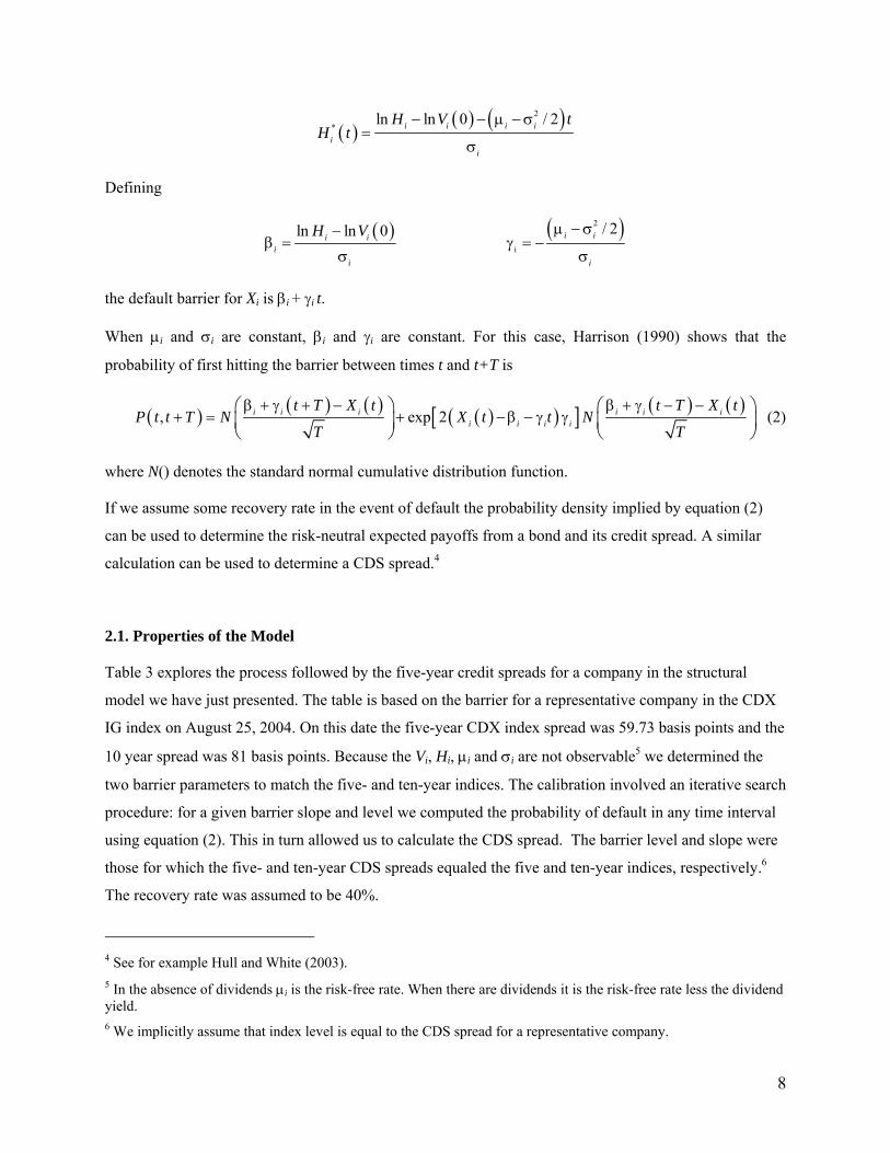
When µi and σi are constant, βi and γi are constant. For this case, Harrison (1990) shows that the

probability of first hitting the barrier between times t and t+T is

( ) ( ) ( ) ( )( )[ ] ( ) ( ), exp 2i i i i i i

i i i i

t T X t t T X tP t t T N X t t N

T T

β + γ + − β + γ − −+ = + − β − γ γ

⎛ ⎞ ⎛ ⎞⎜ ⎟ ⎜ ⎟⎝ ⎠ ⎝ ⎠

(2)

where N() denotes the standard normal cumulative distribution function.

If we assume some recovery rate in the event of default the probability density implied by equation (2)

can be used to determine the risk-neutral expected payoffs from a bond and its credit spread. A similar

calculation can be used to determine a CDS spread.4

2.1. Properties of the Model

Table 3 explores the process followed by the five-year credit spreads for a company in the structural

model we have just presented. The table is based on the barrier for a representative company in the CDX

IG index on August 25, 2004. On this date the five-year CDX index spread was 59.73 basis points and the

10 year spread was 81 basis points. Because the Vi, Hi, µi and σi are not observable5 we determined the

two barrier parameters to match the five- and ten-year indices. The calibration involved an iterative search

procedure: for a given barrier slope and level we computed the probability of default in any time interval

using equation (2). This in turn allowed us to calculate the CDS spread. The barrier level and slope were

those for which the five- and ten-year CDS spreads equaled the five and ten-year indices, respectively.6

The recovery rate was assumed to be 40%.

4 See for example Hull and White (2003). 5 In the absence of dividends µi is the risk-free rate. When there are dividends it is the risk-free rate less the dividend yield. 6 We implicitly assume that index level is equal to the CDS spread for a representative company.

9

The assumption that the barrier level and slope are equal to those for the representative company may

seem to be to be totally unreasonable. However, our experience with both structural and copula models

suggests that setting all credit spreads and pairwise correlations equal to their average values does not

have a significant effect on the valuation of CDO tranches. Practitioners we have spoken to agree with

this observation.

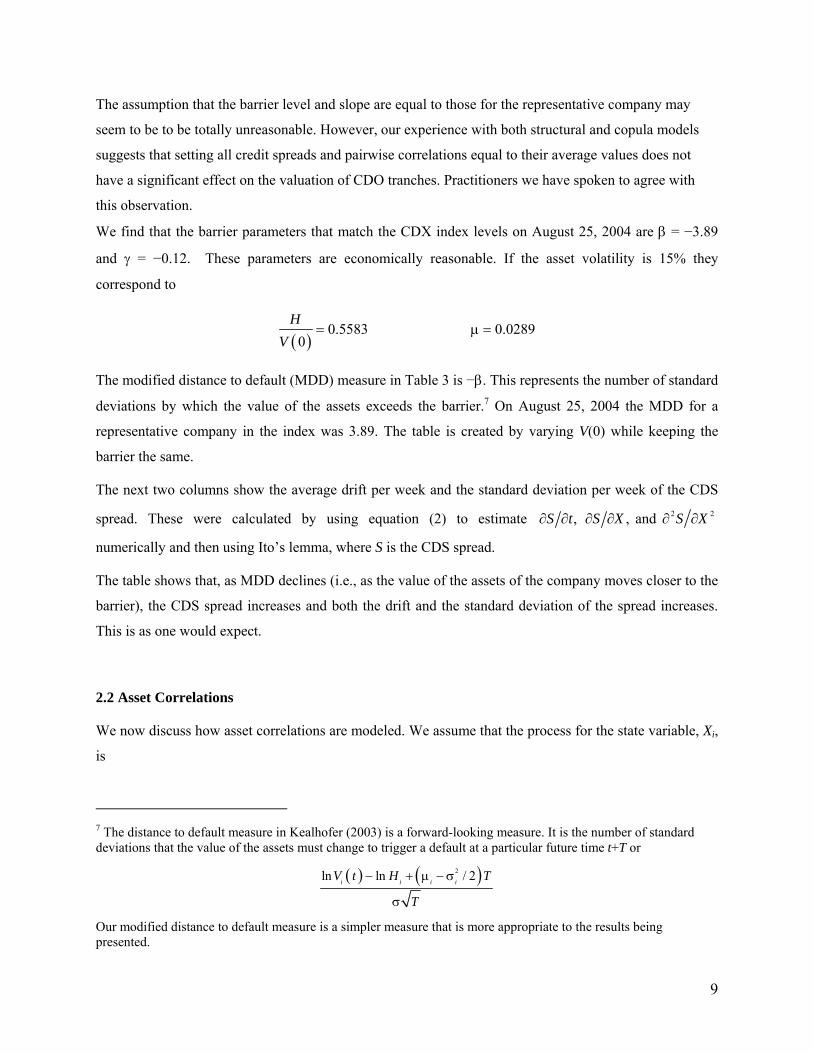
We find that the barrier parameters that match the CDX index levels on August 25, 2004 are β = −3.89

and γ = −0.12. These parameters are economically reasonable. If the asset volatility is 15% they

correspond to

( )0.5583 0.0289

0H

V= µ =

The modified distance to default (MDD) measure in Table 3 is −β. This represents the number of standard

deviations by which the value of the assets exceeds the barrier.7 On August 25, 2004 the MDD for a

representative company in the index was 3.89. The table is created by varying V(0) while keeping the

barrier the same.

The next two columns show the average drift per week and the standard deviation per week of the CDS

spread. These were calculated by using equation (2) to estimate 2 2, , and S t S X S X∂ ∂ ∂ ∂ ∂ ∂

numerically and then using Ito’s lemma, where S is the CDS spread.

The table shows that, as MDD declines (i.e., as the value of the assets of the company moves closer to the

barrier), the CDS spread increases and both the drift and the standard deviation of the spread increases.

This is as one would expect.

2.2 Asset Correlations

We now discuss how asset correlations are modeled. We assume that the process for the state variable, Xi,

is

7 The distance to default measure in Kealhofer (2003) is a forward-looking measure. It is the number of standard deviations that the value of the assets must change to trigger a default at a particular future time t+T or

( ) ( )2ln ln / 2i i i iV t H T

T

− + µ − σ

σ

Our modified distance to default measure is a simpler measure that is more appropriate to the results being presented.

10

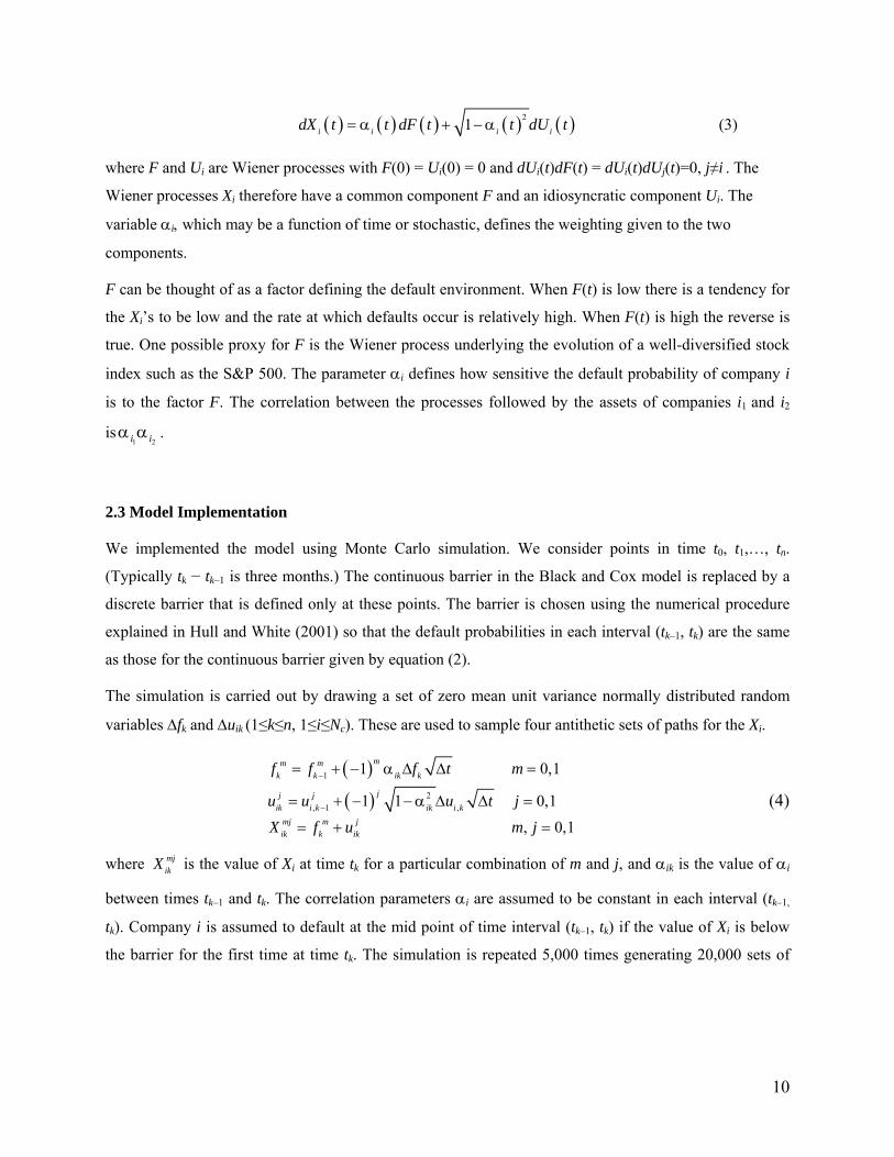
( ) ( ) ( ) ( ) ( )21i i i idX t t dF t t dU t= α + − α (3)

where F and Ui are Wiener processes with F(0) = Ui(0) = 0 and dUi(t)dF(t) = dUi(t)dUj(t)=0, j≠i . The

Wiener processes Xi therefore have a common component F and an idiosyncratic component Ui. The

variable αi, which may be a function of time or stochastic, defines the weighting given to the two

components.

F can be thought of as a factor defining the default environment. When F(t) is low there is a tendency for

the Xi’s to be low and the rate at which defaults occur is relatively high. When F(t) is high the reverse is

true. One possible proxy for F is the Wiener process underlying the evolution of a well-diversified stock

index such as the S&P 500. The parameter αi defines how sensitive the default probability of company i

is to the factor F. The correlation between the processes followed by the assets of companies i1 and i2

is21 ii αα .

2.3 Model Implementation

We implemented the model using Monte Carlo simulation. We consider points in time t0, t1,…, tn.

(Typically tk − tk–1 is three months.) The continuous barrier in the Black and Cox model is replaced by a

discrete barrier that is defined only at these points. The barrier is chosen using the numerical procedure

explained in Hull and White (2001) so that the default probabilities in each interval (tk–1, tk) are the same

as those for the continuous barrier given by equation (2).

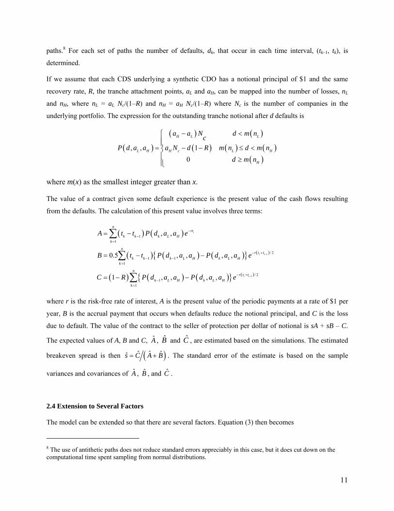
The simulation is carried out by drawing a set of zero mean unit variance normally distributed random

variables ∆fk and ∆uik (1≤k≤n, 1≤i≤Nc). These are used to sample four antithetic sets of paths for the Xi.

( )( )

1

2, 1 ,

1 0,1

1 1 0,1, 0,1

mm mk k ik k

jj jik i k ik i k

mj m jik k ik

f f f t m

u u u t jX f u m j

−

−

= + − α ∆ ∆ =

= + − − α ∆ ∆ =

= + =

(4)

where mjikX is the value of Xi at time tk for a particular combination of m and j, and αik is the value of αi

between times tk–1 and tk. The correlation parameters αi are assumed to be constant in each interval (tk–1,

tk). Company i is assumed to default at the mid point of time interval (tk–1, tk) if the value of Xi is below

the barrier for the first time at time tk. The simulation is repeated 5,000 times generating 20,000 sets of

11

paths.8 For each set of paths the number of defaults, dk, that occur in each time interval, (tk–1, tk), is

determined.

If we assume that each CDS underlying a synthetic CDO has a notional principal of $1 and the same

recovery rate, R, the tranche attachment points, aL and aH, can be mapped into the number of losses, nL

and nH, where nL = aL Nc/(1–R) and nH = aH Nc/(1–R) where Nc is the number of companies in the

underlying portfolio. The expression for the outstanding tranche notional after d defaults is

( )

( ) ( )

( ) ( ) ( )( )

, , 10

H L L

L H H c L H

H

a a N d m ncP d a a a N d R m n d m n

d m n

− <

= − − ≤ <

≥

⎧⎪⎪⎨⎪⎪⎩

where m(x) as the smallest integer greater than x.

The value of a contract given some default experience is the present value of the cash flows resulting

from the defaults. The calculation of this present value involves three terms:

( ) ( )

( ) ( ) ( ){ } ( )

( ) ( ) ( ){ } ( )

1

1

11

/ 21 1

1

/ 21

1

, ,

0.5 , , , ,

1 , , , ,

i

i i

i i

nrt

k k k L Hk

nr t t

k k k L H k L Hk

nr t t

k L H k L Hk

A t t P d a a e

B t t P d a a P d a a e

C R P d a a P d a a e

−

−

−−

=

− +− −

=

− +−

=

= −

= − −

= − −

∑

∑

∑

where r is the risk-free rate of interest, A is the present value of the periodic payments at a rate of $1 per

year, B is the accrual payment that occurs when defaults reduce the notional principal, and C is the loss

due to default. The value of the contract to the seller of protection per dollar of notional is sA + sB – C.

The expected values of A, B and C, A , B and C , are estimated based on the simulations. The estimated

breakeven spread is then ( )ˆ ˆ ˆs C A B= + . The standard error of the estimate is based on the sample

variances and covariances of A , B , and C .

2.4 Extension to Several Factors

The model can be extended so that there are several factors. Equation (3) then becomes

8 The use of antithetic paths does not reduce standard errors appreciably in this case, but it does cut down on the computational time spent sampling from normal distributions.

12

( ) ( ) ( ) ( ) ( )2

1 1

1F Fn n

i ij j ij ij j

dX t t dF t t dU t= =

= α + − α∑ ∑

where nF is the number of factors and αij is the jth factor loading for company i. The correlation between

the processes followed by the assets of companies i1 and i2 is1 2

1

Fn

i j i jj=

α α∑ .

3. Comparison with the Survival-Time Copula Model

As mentioned earlier, a popular way of modeling the joint default probability of many obligors is to use

the factor-based Gaussian copula model of survival time that was suggested by Gregory and Laurent

(2005). In the simplest form of the model, firm i has a random variable xi associated with it. The xi’s are

related through a single factor model

21i i i ix a M Z a= + − (5)

where ai2 ≤ 1 and M and the Zi’s are independent zero mean unit variance normally distributed random

variables. The correlation between xi and xj is aiaj. This is referred to as the copula correlation.

The xi is related to firm i’s time to default ti by equating cumulative density functions so that

N(xi) = Qi(ti)

where N is the cumulative normal distribution function and Qi is the cumulative distribution function for

ti. In this model the factor M captures all the dependence between default events.

Conditional on a particular value of M the probability that firm i will survive until time t is

( ) ( )[ ]1

21

1i i

i

i

N Q t a MS t M N

a

− −= −

−

⎧ ⎫⎪ ⎪⎨ ⎬⎪ ⎪⎩ ⎭

Conditional on M, survival times are independent. The present values of expected cash inflows and

outflows conditional on M can be calculated and these can be integrated over the probability distribution

of M to obtain their unconditional present values.

The survival time copula model has been extended in a number of ways by authors such as Andersen and

Sidenius (2004), Giesecke (2003), and Hull and White (2004). One approach is to increase the number of

factors. Another is to switch from the Gaussian copula to another copula such as the Student t, Clayton,

Archimedean, Marshall-Olkin, or double t. A third approach is to assume a probability distribution for ai

13

that can be dependent on the factor M. These extensions are reviewed in Burtschell, Gregory, and Laurent

(2005).

The survival time copula model is different from the structural model in that the realization of the

common factor M happens at time zero and governs the default outcomes in all time periods. In other

words the default environment is the same for the whole life of the model (usually five or ten years). The

structural model we described in Section 2 is much richer because the realization of F at time t defines the

default environment at that time. A bad default environment in one year can be followed by a good

default environment in the next year.

In spite of these differences there are some reasons to suppose that the correlation environment generated

by the Gaussian copula model is a reasonable approximation to that given by the structural model.

Consider two companies i and j with cumulative probabilities of default by time t equal to Qi(t) and Qj(t).

As before we define ti and tj as the times to default for the companies. Suppose that the Gaussian copula

correlation is *ijρ . The probability that both companies will default by time t is the joint probability that ti

< t and tj < t. Equivalently it is the probability that

xi < N-1(Qi(t)) and xj < N-1(Qj(t))

where xi and xj are defined by equation (5). This is ( ) ( )( )*, ;i j ijB Q t Q t ρ where ( ), ;B a b ρ is the

cumulative probability in a standardized bivariate normal distribution that the first variable will be less

than a and the second variable will be less than b when the correlation between the two variables is ρ.

Under the structural model the joint probability that the companies will default by time t is the probability

that the values of the assets of both companies have dropped below the barrier by time t. If we ignore the

possibility of the value of a company’s assets dropping below the barrier before time t and recovering to

be above the barrier by time t, this equals the probability that the assets of both companies are below the

barrier at time t. This is ( ) ( )( ), ;i j ijB Q t Q t ρ where ρij is the correlation between the asset price

processes for i and j.

This shows that, if we make the simplifying assumption that once a company’s assets are less than the

barrier they remain less than the barrier, the Gaussian copula model and the structural model give the

same joint probabilities of default by any time t when *ij ijρ = ρ . An extension of the argument shows that,

when this simplifying assumption is made, they give the same joint default probabilities of the time to

default for a set of Nc companies for any value of Nc. This in turn means that the models give rise to the

same default correlation structure and the same pricing for CDO tranches.

14

To test the closeness of the results given by the two models we carry out three tests in the sections that

follow. The results show that the models are very similar. However, it is dangerous to assume from this

that the extensions to the basic Gaussian copula survival time model that have been proposed are

reasonable approximations to the corresponding extensions to the basic structural model. For example

making ai dependent on M in equation (5) is clearly quite different from making αi dependent on F in

equation (3).

3.1 Pairwise Correlations

Zhou (2001b) provides exact analytic results for the joint probability of default of two companies under

the Black and Cox (1976) structural model. As we have just explained, the joint probability of default in

the Gaussian copula model can be calculated from the cumulative bivariate normal distribution function.

In Tables 4 and 5 we compare the joint probabilities of default given by the Gaussian copula model with

those given by the structural model when the same correlation parameter is used.

We fit the structural model to market data on August 25, 2004 as in Section 2.1. In Table 4 we investigate

the effect of changing the MDD while keeping the barrier the same. In Table 5 we investigate the effect of

changing the time horizon considered. In all cases the marginal default probabilities for the Gaussian

copula model and the structural model are the same.

Table 5 shows that the joint probabilities given by the two models are very close. As MDD decreases, the

probability of default increases and the absolute difference between the joint probabilities given by the

two models increases. (This is consistent with the fact that companies far away from the barrier are likely

to cross the barrier toward the end of the period making the Gaussian copula a better approximation than

for companies close to the barrier.). However, the proportional difference decreases. As the correlation

parameter increases, the difference (absolute and proportional) between the two models increases. Table 5

shows that as the time horizon is increased the absolute difference between the joint probabilities given by

the two models increases while the percentage difference decreases. In all cases the Gaussian copula

model overstates the joint probabilities.

3.2 CDO Tranche Pricing

Table 6 compares tranche prices for the structural model with those for the Gaussian copula survival time

model. Again we use a structural model with parameters chosen to match the indices on August 25, 2004.

15

As in the case of the pairwise correlation analysis, the marginal default probabilities for the two models

are the same.

It can be seen that the models produce quite similar results. We measure the difference between the two

models by calculating the mean absolute spread difference (MASD) across tranches. We obtained similar

results using the 10-year CDX data and using iTraxx data. It is clear that from these results and other tests

we have carried out that the Gaussian copula survival time model is a good approximation to the basic

structural model in a wide range of situations. When we increased spreads we found that two models do

diverge, but only very slowly.

3.3 Deltas

It is sometimes assumed that an accurate calculation of deltas for a structural model is impossible. We

have not found this to be the case. Our approach is to perturb the 5- and 10-year index spreads by x basis

points, recalculate the barrier and the marginal default probabilities, and reprice the CDO tranches using

the same sequence of random numbers. The delta is calculated as the change in the breakeven tranche

spread divided by x. To test the robustness of our procedure we used values of x equal to −10, −5, −3, −2,

−1, +1, +2, +3, +5, and +10.

Two alternative deltas can be calculated. For the first delta the perturbed barrier or marginal default

probabilities applies to only one of the 125 firms in the portfolio underlying the CDO. The barrier or

default probabilities for the remaining 124 firms remain unchanged. For the second delta the change is

applied to all the firms in the portfolio.

By comparing the results for different values of x we found that the relationship between tranche spread

and index spread is fairly linear, particularly in the case of the single-name delta. The results for the

structural model using 20,000 trials (5,000 independent paths for F and U) are summarized in Table 7.

Apart from confirming that our approach to calculating delta is fairly robust the table shows that the 125-

name delta is approximately 125 times the one-name delta. This suggests an interesting approach to

calculating a one-name delta when a homogeneous model is used. The common CDS spread is shifted

by, say, 10 basis points and the resulting 125-name delta is divided by 125.

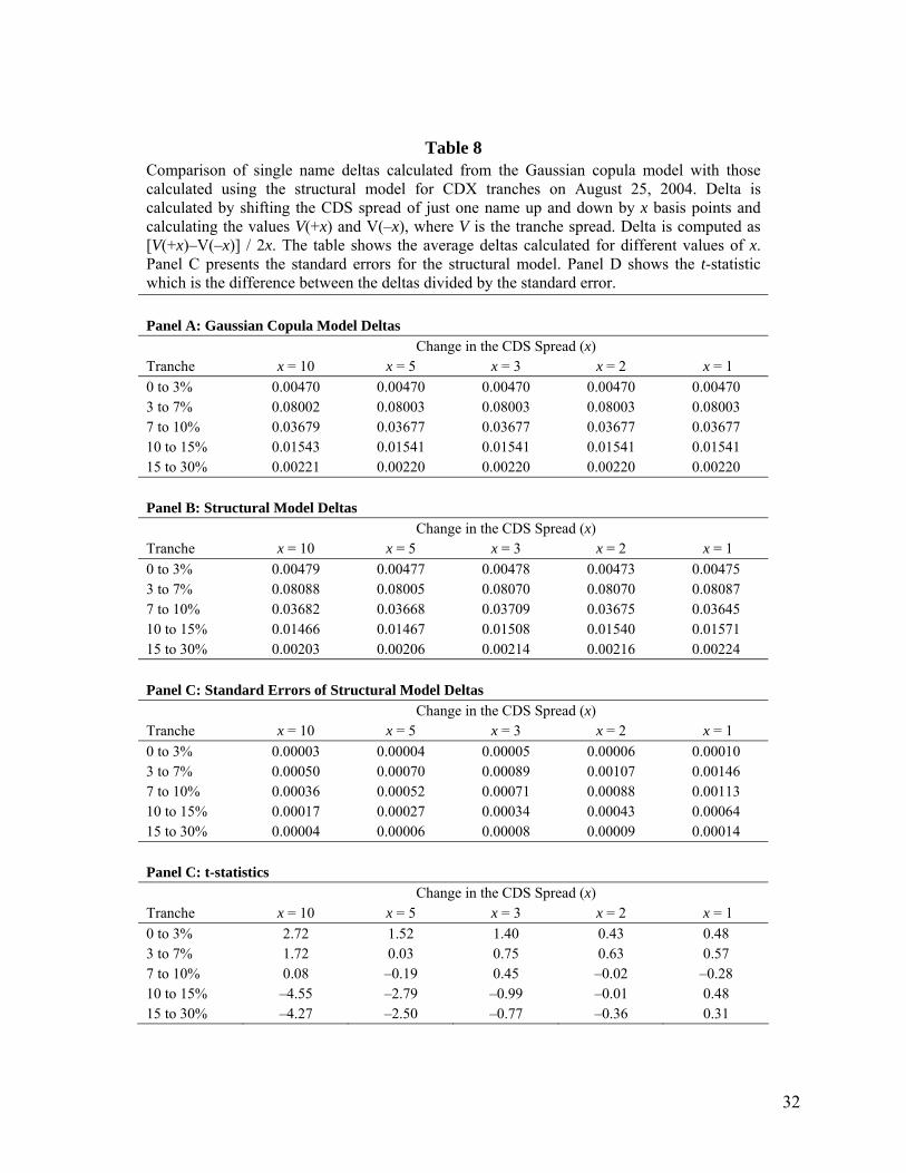
Table 8 compares the structural model delta with the delta calculated from the Gaussian copula model.9

The standard error of the estimate was calculated by repeating the Monte Carlo simulation several

9 The latter required the bucketing approach to calculating the loss distribution explained by Andersen et al (2003) and Hull and White (2004).

16

hundred times. It can be seen that the Gaussian copula deltas are very close to the structural model deltas.

This provides further evidence that the two models are very close to each other.

4. Data

The data on CDX and iTraxx index tranches was provided by GFI, a large credit derivatives broker. It

covers the period from January 2, 2004 to December 21, 2004 and consists of intraday bid and offer

quotes as well as trades for CDO tranches. We computed the daily bid as the average of all intra-day bids.

The daily offer quote was computed similarly. We used the daily mid-quote (the average of daily bid and

offer quotes) as the daily observation in the sample.

Table 2 presents summary statistics on tranche spreads and bid-ask spreads for 5 year and 10 year index

tranches. In general CDX and iTraxx tranche spreads decreased over time. For example the mean 5 year

CDX equity tranche spread for the first half a year (1/1/2004-30/6/2004) was 41.5%. It decreased to

37.9% in the second half. The spreads for the other five-year CDX tranches decreased from 332.3bp,

118.2bp, 51.7bp, and 13.8bp to 272.2bp, 105.1bp, 37.8bp and 11.6bp, respectively.10

The bid-ask spreads also fell over time, consistent with an increase in liquidity in this market. For

example, in the case of CDX, the mean bid-ask spread for the five-year equity tranche for the first half a

year was 2.4% and decreased to 1.5% in the second half. Similarly the mean bid-ask spreads for the 5Y

CDX 3-7%, 7-10%, 10-15% and 15-30% tranches decreased from 43.6bp, 11.8bp, 13.1bp, 7.6bp to 9.6bp,

6.1bp, 6.3bp and 3.1 bp, respectively.

The data is incomplete in that not all the quotes shown in Table 1 are available for all days. In our

analysis we considered only days where a complete set of bids and offers was available, that is,

observations on all five tranches and the index for both five- and ten-year maturities. There were 51 such

days for iTraxx IG and 60 such days for CDX IG.

In order to fit the structural model to a set of CDX or iTraxx quotes on a particular day we must estimate

the following: the risk-free zero curve, the asset correlation, the barrier slope, and the barrier level. We

downloaded risk-free zero curves from Bloomberg. The applicable risk-free zero curve for CDX IG is the

USD zero curve and the applicable zero curve for iTraxx IG is the EUR zero curve. In the next section,

we describe how the correlation parameter was chosen in the various tests we carried out.

10 These numbers are not included in the table.

17

The barrier level and slope were chosen to be the same for all companies and consistent with the quoted

five- and ten-year indices.11 For a given barrier we can calculate the probability of default in any time

interval using equation (2). This in turn allows us to calculate the CDS spread. The barrier level and

slope were those for which the five- and ten-year CDS spreads equaled the five and ten-year indices,

respectively.12

5. Empirical Analysis

We now test how well the structural model fits CDX IG market data on the days for which a complete set

of data is available. The results for iTraxx IG are similar.

5.1 Base Case

In our base case the correlation parameter, αi(t) and recovery rate, R, are independent of the default

environment parameter, F(t). For the first test αi(t) was the same for all i and t so that the pricing of the

five-year equity tranche matched the market.13 We then compared the model’s pricing of the other five-

year tranches and all ten-year tranches with the market. These results are referred to as Base Case (5) in

our tables. As a second test, we assumed that αi(t) is the same for all i and is a step function, having one

value up to five years and another value beyond five years. The step function is chosen to match both the

five-year and the ten-year equity tranches. The results comparing model and market pricing for other

tranches for this test are referred to as Base Case (5, 10) in our tables.

The recovery rate, R, was assumed to be constant and 40% for all obligors. This is consistent with

research in Varma and Cantor (2004).

11 This approach can be extended so that a non-linear barrier that is consistent with a complete term structure of default probabilities or CDS spreads is developed. 12 Under our assumption that default probabilities are the same for all companies the CDS spread equals the index. The calculation of CDS spreads from default probabilities and recovery rates is described in, for example, Hull and White (2003). We assumed a recovery rate of 40%. This is consistent with Varma and Cantor (2004). Our definition of recovery rate is the standard one: value of cheapest to deliver bond as a percent of face value. 13 We matched the equity tranche because the pricing of this tranche is highly sensitive to the value of the correlation parameter.

18

5.2. Stochastic Correlation

There is some empirical evidence to suggest that asset correlations are stochastic and increase when

default rates are high. For example Servigny and Renault (2002), who look at historical data on defaults

and ratings transitions to estimate default correlations, find that the correlations are higher in recessions

than in expansion periods. Das, Freed, Geng and Kapadia (2004) employ a reduced form approach and

compute the correlation between default intensities. They conclude that default correlations increase when

default rates are high. Ang and Chen (2002) find that the correlation between equity returns is higher

during a market downturn.

To test the impact of stochastic correlation we assumed that the correlation parameter αik applicable

between times tk–1 and tk is drawn from a beta distribution. The beta distribution was the same for all i. We

used a Gaussian copula model to build in dependence between the value sampled for αik and the value

sampled for Fk–1. The copula correlation was chosen as 0.5− .14 This is achieved by making the value

sampled for αk the same fractile of a beta distribution as ( )1 10.5 0.5k kF − −− − ξ is of a normal

distribution, where the ξ ’s have normal distributions with zero mean and unit variance rate and are

independent of the F’s and U’s.

Our tests for the stochastic correlation model are similar to those for the base case model. For the first

test, the mean of the beta distribution, α , is assumed to be the same for ten years and is chosen to match

the 5-year equity tranche. The results from this test are referred to as “Stochastic Corr. (5)”. For the

second test α is a step function, chosen to match both the five-year and the ten-year equity tranche. The

results for the second test are referred to as “Stochastic Corr. (5, 10)”.

5.3 Stochastic Recovery Rate

Altman et al. (2005) and Cantor, Hamilton, and Ou (2002) show that recovery rates are negatively

dependent on default rates. To test the impact of this we assumed that the recovery rate, Rk, applicable

between times tk–1 and tk has a beta distribution and used a Gaussian copula model to build in dependence

between it and Fk-1. In this case the copula correlation was chosen to be 0.5+ .15 As before this means

14 A negative correlation between the α’s and the F’s corresponds to a positive correlation between α and the default rates. 15 A positive correlation between the recovery rate and the F’s corresponds to a negative correlation between recovery rates and default rates.

19

that value sampled for αk is the same fractile of a beta distribution as ( )11 5.05.0 −− + kkF ξ is of a

normal distribution, where the ξ ’s have normal distributions with zero mean and unit variance rate and

are independent of the F’s and U’s.

The mean of the recovery rate distribution, R , was chosen so that the expected recovery given default is

0.4. This does not mean that 0.4.R = In practice a higher value of R (about 0.47) was necessary because

the recovery rates tend to be observed when the factor F is low.

5.4 Stochastic Volatility

Hull and White (2004) and Burtschell, Gregory and Laurent (2005) show that a double-t copula model

where both the common factor and the idiosyncratic factor have a t-distribution with 4 degrees of freedom

fits the market prices well. These findings suggest that market prices are consistent with heavy tails for

the common factor and the idiosyncratic factor.

To investigate this in the context of the structural framework, we consider a third extension to the base

case model where both the common factor F and the idiosyncratic factor U have stochastic volatilities.

Specifically we assume that each of the factors is drawn from a mixture of Wiener processes with

different variance rates. F is assumed to be drawn with probability pF,1 from a process with variance rate

VF,1 and probability (1 – pF,1) from a process with variance rate VF,2. The expected variance of F is 1. U is

treated similarly. The parameters we chose are VF,1=1.5, VF,2=0.5, pF,1=0.5; VU,1 =1.5, VU,2=0.5, pU,1=0.5.

5.5 The Results

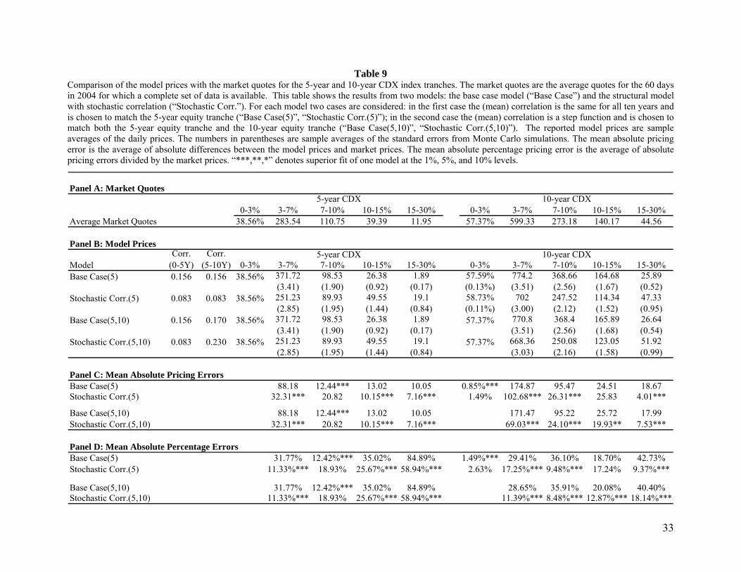
Our results are shown in Tables 9 to 12. Table 9 compares the model prices from the base case model and

the stochastic correlation model with the market quotes for CDX IG. Table 10 compares model prices

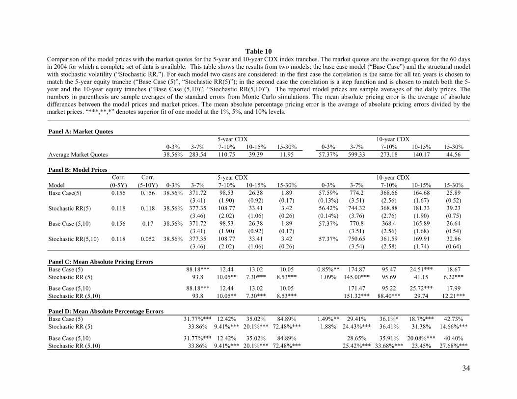
from the base case model and the stochastic recovery rate model with the market quotes for CDX IG.

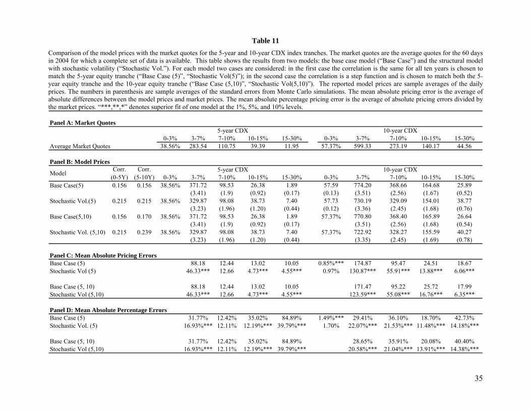
Table 11 compares model prices from the base case model and the stochastic volatility model with the

market quotes for CDX IG.16 The overall fit of the models is examined in Table 12.

Table 9 shows that Base Case (5), where the correlation parameter is constant and fits the market price of

the five-year equity tranche, greatly overprices the mezzanine tranche and greatly under prices the most

senior tranche. Stochastic Corr. (5), where the mean correlation is constant and fits the market price of the

five-year equity tranche, brings pricing closer to that in the market for both these tranches. Base Case (5)

sometimes does a better job at pricing intermediate tranches than Stochastic Corr. (5) (for example, the 16 Similar tests to those in Tables 9, 10 and 11 were carried out for iTraxx. The results were similar.

20

7% to 10% tranche) but the improvement is relatively small. The results from comparing Base Case

(5, 10) where the correlation is a step function with Stochastic Corr. (5, 10) are similar.

Table 10 shows the results from the base case and the stochastic recovery models are fairly close. This is

a little surprising. A possible explanation is that the positive effect on the fit of the model caused by the

negative correlation of recovery rate and default rate is counteracted by the negative effect on the fit of

the lower default correlation necessary to match the equity tranche.

From Table 11 we see that Stochastic Vol (5) does significantly better than Base Case (5) and Stochastic

Vol (5, 10) does significantly better than Base Case (5,10) for almost all tranches. The one exception is

that Base Case (5) outperforms Stochastic Vol (5) for the 10-year equity tranche. But the extent of the out

performance is relatively small.

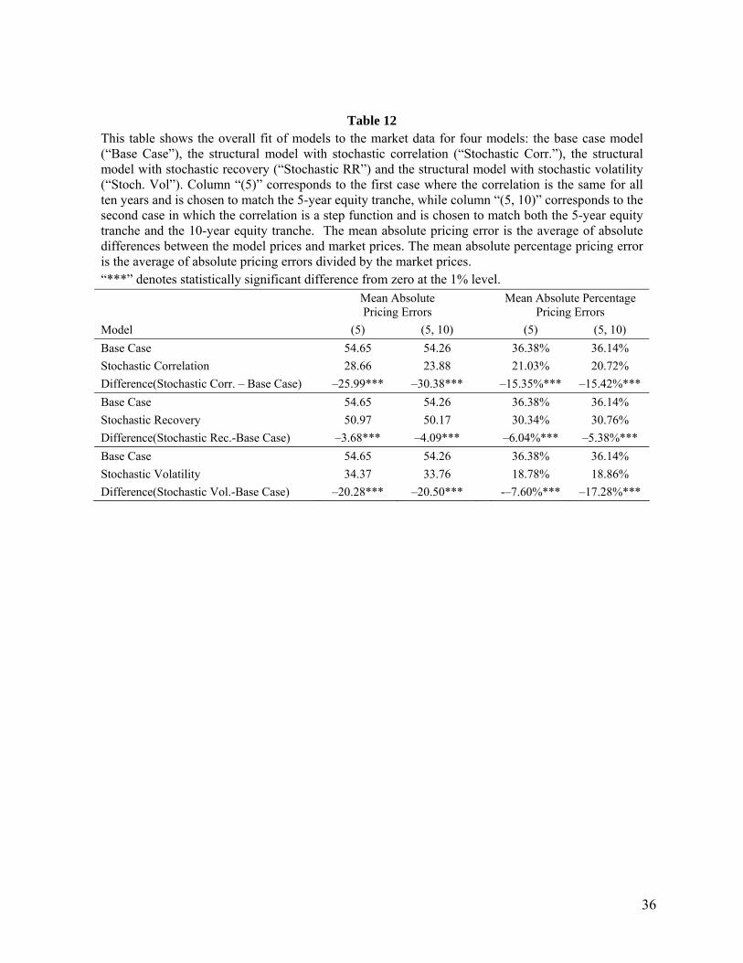
Table 12 compares the overall fit of the models by computing the mean absolute pricing errors and the

mean absolute percentage pricing errors. The mean absolute pricing error is the average of absolute

differences between the model prices and market prices. The mean absolute percentage pricing error is the

average of absolute pricing errors divided by the market prices. The statistical significance of the mean

difference between the pricing errors from the two models is tested using both a parametric t-test and a

non-parametric bootstrap test. All three (5) and (5, 10) extensions of the Base Case model provide an

improvement over the Base Case model at the 1% level. However, the economic significance of the

results for the stochastic correlation model and the stochastic volatility model is much greater than that for

the stochastic recovery rate model.

The stochastic correlation model does a better job than the stochastic volatility model when mean

absolute pricing errors are used but slightly worse when mean absolute percentage pricing errors are used.

This is because the stochastic volatility model tends to be closer in absolute terms on senior tranches

where the quote is low and less close on junior tranches where the quote is high.

6. Conclusions

We have proposed a structural model similar to that in Black and Cox (1976) for valuing correlation-

dependent credit derivatives. The correlation between the assets of different companies is determined by

one or more common factors.

The basic Gaussian copula survival time model provides a good approximation to our base-case structural

model when the correlation parameter in the model is set equal to the asset correlation in the structural

model. Even for relatively large credit spreads the prices given by the two models are fairly close. The

21

advantage of the structural model is that it provides a way of simultaneously modeling credit rating

changes and defaults. Also it is possible to make extensions to the model while maintaining its economic

integrity as a structural model.

The basic structural model does not provide a good fit to the market prices of CDO tranches. When the

correlation parameter is chosen to match the price of the equity tranche, the mezzanine tranche is

overpriced and the other tranches (particularly the most senior tranche) are under priced.

The basic structural model assumes that asset correlations are constant. Empirical evidence suggests that

asset correlations are positively related to default rates. We therefore tested whether an extension of the

structural model that incorporates this positive relationship fits market prices better than the basic

structural model. We found that there is a significantly better fit at the 1% level. Our results suggest that

further research quantifying the relationship between asset correlations and default rates could lead to

better pricing models. Another model where the common factor and the idiosyncratic factor in the

structural model have heavy tails produced approximately the same improvement over the basic structural

model as the stochastic correlation model.

There is a growing body of empirical evidence to show that recovery rates are negatively correlated with

default rates. Surprisingly, an extension of the basic structural model to incorporate this phenomenon

produces only a marginally better fit to market prices. Although statistically significant this is not

economically significant.

Hull and White (2006) show that a copula model can be developed by simply specifying a number of

different hazard rate term structures and assigning probabilities to them (the implied copula approach).

They provide a way of choosing the hazard rate term structures and their associated probabilities so that

market quotes are matched. An interesting idea is to extend their methodology so that a copula model

consistent with a structural model is identified. This would enable a much faster way of implementing a

structural model to be developed. This is an area for further research.

22

References

Altman, E. I., B. Brady, A. Resti and A. Sironi, 2005, “The Link between Default and Recovery Rates:

Theory, Empirical Evidence, and Implications,” Journal of Business, 78, 2203–2228.

Andersen, L., 2000, “A Simple Approach to Pricing Bermudan Options in the Multifactor LIBOR Market

Model,” Journal of Computational Finance, 3, 2 (Winter), 1-32.

Andersen, L. and J. Sidenius, 2004, “Extensions to the Gaussian Copula: Random Recovery and random

Factor Loadings,” Journal of Credit Risk, 1, 1 (Winter), 29-70.

Andersen, L., J. Sidenius, and S. Basu, 2003, “All Your Hedges in One Basket,” RISK, November.

Ang, A. and J. Chen, 2002, “Asymmetric Correlations of Equity Portfolios,” Journal of Financial

Economics, Vol. 63, 443-494

Black, F. and J. Cox, 1976, “Valuing Corporate Securities: Some Effects of Bond Indenture Provisions,”

Journal of Finance, 31, 351-67.

Burtschell, X., J. Gregory and J.-P. Laurent, 2005, “A Comparative Analysis of CDO pricing models,”

Working Paper, BNP Paribas.

Cantor, R., D.T. Hamilton, and S. Ou, 2002, "Default and Recovery Rates of Corporate Bond

Issuers" Moody's Investors Services, February.

Das, S. R., L. Freed, G. Geng and N. Kapadia, 2006, “Correlated Default Risk,” Journal of Fixed Income,

16, 2, 7-32.

Duffie, D. and N. Gârleanu, 2001, “Risk and Valuation of Collateralized Debt Obligations,” Financial

Analysts Journal, 57 (January/February), 41-59.

Geske, R., 1977, “The Valuation of Corporate Liabilities as Compound Options,” Journal of Financial

and Quantitative Analysis, 5, 541-52.

23

Giesecke, K., 2003, “A Simple Exponential Model for Dependent Defaults,” Journal of Fixed Income,

December, 74-83.

Gregory, J. and J.-P. Laurent, 2005, “Basket Default Swaps, CDO’s and Factor Copulas,” Journal of Risk,

7, 4 (Summer), 103-22.

Harrison, J. M., 1990, Brownian Motion and Stochastic Flow Systems, Krieger Publishing Company.

Hull, J. and A. White, 2003, “The Valuation of Credit Default Swap Options,” Journal of Derivatives, 10,

3 (Spring), 40-50

Hull, J., and White, A., 2001, “Valuing Credit Default Swaps II: Modeling Default Correlations,” Journal

of Derivatives, Vol. 8, No. 3, 12-22

Hull, J. and White, A., 2004, “Valuation of a CDO and nth to Default CDS Without Monte Carlo

Simulation,” Journal of Derivatives, Vol. 12, No. 2, 8-23.

Hull, J. and White A., 2006, “Valuing Credit Derivatives Using an Implied Copula Approach,” Journal

of Derivatives, Forthcoming.

Kakodkar, A. and B. Martin, 2004, “The Standardized Tranche Market Has Come Out of Hiding,”

Journal of Structured Finance, Fall, p. 76-81.

Kealhofer, S., 2003, “Quantifying Default Risk I: Default Prediction,” Financial Analysts Journal, 59, 1,

33-44.

Kim, I. J., Ramaswamy, K., and Sundaresan, S. M., 1993, “Valuation of Corporate Fixed-Income

Securities,” Financial Management, Autumn, p. 117-131.

Leland, H. E., 1994, “Risky Debt, Bond Covenants and Optimal Capital Structure,” Journal of Finance,

Vol. 49, 1213-1252.

Leland, H. E. and Toft, K. B., 1996, “Optimal Capital Structure, Endogenous Bankruptcy and the Term

Structure of Credit Spreads,” Journal of Finance, Vol. 50, 789-819.

24

Li, D.X., 2000, “On Default Correlation: A Copula Approach,” Journal of Fixed Income, Vol. 9, March,

p. 43-54.

Longstaff, F. A. and Schwartz, E. S., 1995, “A Simple Approach to Valuing Risky Fixed and Floating

Rate Debt,” Journal of Finance, Vol. 50, No. 3, 789-819.

Longstaff, F.A. and Schwartz, E.S., 2001, “Valuing American Options by Simulation: A Simple Least

Squares Approach,” Review of Financial Studies, 14, 1 (Spring ), 113-47.

Longstaff, F. A. and Rajan, A., 2006, “An Empirical Analysis of the Pricing of Collateralized Debt

Obligations,” Working Paper, UCLA Anderson School of Management

Merton, R., 1974, “On the Pricing of Corporate Debt: the Risk Structure of Interest Rates,” Journal of

Finance, Vol. 29, 449-470.

Servigny, A. and O. Renault, 2002, “Default Correlation: Empirical Evidence,” Working Paper, Standard

and Poors.

Varma, P. and R. Cantor, 2004, “Determinants of Recovery Rates on Defaulted Bonds and Loans for

North American Corporate Issuers: 1983-2003,” Moody’s Investors Services, December.

Zhou, C., 2001a, “The Term Structure of Credit Spreads with Jump Risk,” Journal of Banking and

Finance, Vol. 25, 2015-2040.

Zhou, C., 2001b, “An Analysis of Default Correlations and Multiple Defaults,” Review of Financial

Studies, Vol. 14, No. 2, 555-576.

25

Table 1 Quotes for CDX IG and iTraxx IG Tranches on August 25, 2004. The quote for the 0% to 3% tranche is the upfront payment as a percentage of the notional principal that is paid in addition to 500 basis points per year. Quotes for all other tranches and the index are in basis points per year. Source: GFI CDX IG Tranches 0% to 3% 3% to 7% 7% to 10% 10% to 15% 15% to 30% Index 5-year Quotes 40.02 295.71 120.50 43.00 12.43 59.73 10-year Quotes 58.17 632.00 301.00 154.00 49.50 81.00

iTraxx IG Tranches 0% to 3% 3% to 6% 6% to 9% 9% to 12% 12% to 22% Index 5-year Quotes 24.10 127.50 54.00 32.50 18.00 37.79 10-year Quotes 43.80 350.17 167.17 97.67 54.33 51.25

26

Table 2

Descriptive Statistics on Daily Mid-Quotes and Bid-Ask Spreads for CDX and iTraxx tranches between January 2 and December 21, 2004. The daily bid for each tranche is computed as the average of all intra-day bids for that tranche. The daily offer quote was computed similarly. The mid-quote is the average of daily bid and daily ask. The bid-ask spread is defined as the difference between the daily ask and daily bid, while the percentage bid-ask spread is the ratio of the bid-ask spread and the mid-quote. Panels A present the time-series means and standard deviations of daily tranche mid-quotes. Panels B and C present the same statistics for bid-ask spreads and percentage bid-ask spreads. CDX Tranches 5Y Tranches 10Y Tranches 0-3% 3-7% 7-10% 10-15% 15-30% 0-3% 3-7% 7-10% 10-15% 15-30% Panel A: Mid Quotes Mean 39.6 301.4 111.4 44.4 12.7 57.0 597.8 270.7 145.2 43.4 Std. Dev. 3.6 57.9 24.1 10.7 2.2 2.3 70.7 62.1 36.1 8.1 No. Obs. 214 214 215 207 210 84 101 107 106 86 Panel B: Bid-Ask Spreads Mean 1.9 26.1 8.8 9.5 5.2 3.7 37.1 29.0 20.9 9.6 Std. Dev. 1.0 24.8 5.0 5.0 2.8 1.4 16.7 14.5 6.4 4.1 Panel C: Percentage Bid-Ask Spreads Mean 4.8% 8.4% 8.3% 21.7% 41.0% 6.5% 6.2% 10.7% 15.0% 22.5% Std. Dev. 2.5% 7.8% 5.5% 10.2% 20.5% 2.4% 2.8% 5.1% 5.2% 9.1% iTraxx Tranches 5Y Tranches 10Y Tranches 0-3% 3-6% 6-9% 9-12% 12-22% 0-3% 3-6% 6-9% 9-12% 12-22% Panel A: Mid Quotes Mean 25.4 148.5 56.9 36.6 17.4 45.1 376.7 165.5 95.4 50.2 Std. Dev. 3.3 28.8 16.0 9.1 3.3 4.0 37.8 26.5 17.1 9.8 No. Obs. 131 132 131 130 131 68 63 64 61 62 Panel B: Bid-Ask Spreads Mean 1.4 7.4 5.8 6.0 2.9 3.3 37.5 21.1 20.4 17.6 Std. Dev. 0.8 4.6 2.6 1.6 1.4 1.0 7.3 8.6 5.1 2.7 Panel C: Percentage Bid-Ask Spreads Mean 5.4% 4.9% 10.2% 16.5% 16.2% 7.3% 10.0% 12.6% 21.4% 36.5% Std. Dev. 3.0% 2.3% 3.2% 3.4% 5.2% 2.3% 2.2% 4.9% 4.5% 9.4%

27

Table 3 Five-year credit spread dynamics given by the structural model for a representative CDX IG company. The model parameters (barrier level, β, and slope, γ, for the representative company) are calibrated to the five-year and ten-year CDX index levels on August 25, 2004. The Modified Distance to Default (MDD) represents the number of standard deviations by which the asset value exceeds the default barrier ( (ln (0) ln )MDD V H= −β = − σ ). The table is created by varying MDD (i.e. the barrier level) and keeping the barrier slope the same. The CDS spread, drift and standard deviation are all expressed in basis points. Modified Distance to

Default (MDD) 5Y CDS Spread Drift of 5Y Credit Spread (per week)

Std Dev of 5Y credit spread (per week)

2.50 251.64 1.7 34.3 3.00 153.01 0.9 21.5 3.50 91.04 0.5 13.5 4.00 52.54 0.2 8.3 4.50 29.24 0.1 4.9 5.00 15.64 0.1 2.8

28

Table 4 This table compares the five-year joint default probability of two correlated issuers implied by the structural model with that implied by the Gaussian copula model. The comparison is performed for different levels of issuers’ riskiness (as represented by the Modified Distance to Default) and different levels of correlation between the issuers’ asset values. The structural model parameters are fitted to August 25th data on CDX indices. The five-year joint default probabilities from the structural model (presented in Panel A) are computed using the analytical formulas in Zhou (2001). Panel B presents the joint five-year default probabilities of two-issuers as implied by the Gaussian copula model. These are calculated from the cumulative bivariate normal distribution function under the assumptions that the marginal default probabilities of the two issuers are matched to those in the structural model and the copula correlation is equal to the asset returns correlation in the structural model.

Panel A: Structural Model Modified Distance to Default (MDD)

Correlation 2 2.5 3 3.5 4 4.5 5 0.1 15.11% 7.97% 3.91% 1.78% 0.75% 0.29% 0.10% 0.2 16.48% 9.05% 4.65% 2.23% 1.00% 0.42% 0.16% 0.3 17.91% 10.19% 5.46% 2.74% 1.29% 0.57% 0.24% 0.4 19.42% 11.41% 6.34% 3.32% 1.64% 0.76% 0.33% 0.5 21.02% 12.72% 7.31% 3.98% 2.05% 1.00% 0.46%

Panel B: Gaussian Copula Model MDD

Correlation 2 2.5 3 3.5 4 4.5 5 0.1 15.21% 8.03% 3.95% 1.80% 0.76% 0.29% 0.11% 0.2 16.67% 9.17% 4.72% 2.27% 1.02% 0.42% 0.16% 0.3 18.18% 10.37% 5.56% 2.80% 1.32% 0.58% 0.24% 0.4 19.75% 11.63% 6.47% 3.40% 1.68% 0.78% 0.34% 0.5 21.41% 12.98% 7.47% 4.07% 2.10% 1.02% 0.47%

29

Table 5 This table compares the joint default probability of two correlated issuers implied by the structural model with that implied by the Gaussian copula model. The comparison is performed for different time horizons and different levels of correlation between the issuers’ asset values. The structural model parameters are fitted to August 25th data on CDX indices. The joint default probabilities from the structural model (presented in Panel A) are computed using the analytical formulas in Zhou (2001). Panel B presents the joint default probabilities of two-issuers as implied by the Gaussian copula model. These are calculated from the cumulative bivariate normal distribution function under the assumptions that the marginal default probabilities of the two issuers are matched to those in the structural model and the copula correlation is equal to the asset returns correlation.

Panel A: Structural Model Maturity (in years)

Correlation 1 3 5 7 10 15 20 0.1 0.00% 0.10% 0.92% 2.52% 5.65% 11.16% 16.17% 0.2 0.00% 0.16% 1.21% 3.09% 6.56% 12.41% 17.58% 0.3 0.00% 0.23% 1.55% 3.72% 7.53% 13.71% 19.03% 0.4 0.00% 0.32% 1.94% 4.42% 8.58% 15.09% 20.56% 0.5 0.00% 0.45% 2.40% 5.21% 9.73% 16.56% 22.18%

Panel B: Gaussian Copula Model Maturity (in years)

Correlation 1 3 5 7 10 15 20 0.1 0.00% 0.10% 0.93% 2.55% 5.70% 11.24% 16.28% 0.2 0.00% 0.16% 1.23% 3.14% 6.65% 12.56% 17.78% 0.3 0.00% 0.23% 1.58% 3.79% 7.67% 13.93% 19.31% 0.4 0.00% 0.33% 1.98% 4.52% 8.76% 15.36% 20.91% 0.5 0.00% 0.46% 2.46% 5.33% 9.94% 16.89% 22.59%

30

Table 6 Comparison of the 5-year CDX IG tranche prices computed from the structural model with the prices from the Gaussian Copula model. The 0% to 3% tranche is quoted as the percentage upfront payment required on the assumption that subsequent payments will be 500 basis points per year. The other tranches are quoted as basis points per year. The structural model parameters are fitted to August 25th data on CDX indices. Panel A presents the tranche prices implied by the structural model for different asset correlation values. The numbers in parentheses are standard errors of the tranche price estimates from the structural model. Panel B presents the tranche prices implied by the Gaussian copula model. The marginal default probabilities in the Gaussian copula model are matched to those in the structural model and the copula correlation is equal to the asset returns correlation.

Panel A: Structural Model Prices Tranches

Correlation 0-3% 3-7% 7-10% 10-15% 15-30% 0.1 46.2% (0.16%) 376.0 (3.3) 66.9 (1.5) 11.0 (0.6) 0.3 (0.1) 0.2 37.1% (0.19%) 407.5 (3.7) 135.1 (2.3) 45.8 (1.3) 5.1 (0.3) 0.3 29.4% (0.20%) 407.4 (3.9) 175.8 (2.7) 81.4 (1.8) 16.2 (0.7) 0.4 22.5% (0.21%) 393.1 (3.9) 198.9 (2.9) 109.7 (2.1) 31.2 (1.0) 0.5 16.1% (0.21%) 369.6 (3.9) 210.8 (3.0) 130.2 (2.4) 47.8 (1.3)

Panel B: Gaussian Copula Model Prices Tranches

Correlation 0-3% 3-7% 7-10% 10-15% 15-30% 0.1 45.8% 383.4 70.9 12.0 0.4 0.2 36.5% 414.8 140.8 48.7 5.5 0.3 28.7% 413.0 182.1 84.8 17.2 0.4 21.7% 396.5 205.5 114.3 32.3 0.5 15.4% 370.9 218.3 132.4 50.1

Panel C: Differences: Structural – Gaussian Copula Tranches

Correlation 0-3% 3-7% 7-10% 10-15% 15-30% 0.1 0.4% –7.4 –4.0 –1.0 0.0 0.2 0.6% –7.3 –5.8 –2.8 –0.4 0.3 0.7% –5.7 –6.3 –3.4 –1.1 0.4 0.8% –3.4 –6.6 –4.6 –1.1 0.5 0.7% –1.3 –7.5 –2.2 –2.3

31

Table 7 Deltas for the breakeven spreads of CDX tranches calculated from a Monte Carlo implementation of the structural model on August 25, 2004. Delta is calculated by shifting the CDS spread up and down by x basis points and calculating the values V(+x) and V(–x), where V is the tranche spread. Delta is computed as [V(+x)–V(–x)] / 2x. The table shows the average deltas calculated for different values of x. Panel A presents the 1-name deltas for CDX tranches. These are computed by assuming that the shift in the CDS spread is applied to just one company. Panel B presents the 125-name deltas computed by shifting the CDS spreads of all 125 companies. Panel C shows the ratio of the 125-name delta to the 1-name delta. Panel A: Tranche Deltas Calculated by Perturbing the CDS Spread for One Name Change in the CDS Spread of One Name (x) Tranche x = 10 x = 5 x = 3 x = 2 x = 1 0 to 3% 0.00470 0.00470 0.00470 0.00470 0.00470 3 to 7% 0.08002 0.08003 0.08003 0.08003 0.08003 7 to 10% 0.03679 0.03677 0.03677 0.03677 0.03677 10 to 15% 0.01543 0.01541 0.01541 0.01541 0.01541 15 to 30% 0.00221 0.00220 0.00220 0.00220 0.00220 Panel B: Tranche Deltas Calculated by Perturbing the CDS Spread for All 125 names Change in the CDS Spreads of Each of the 125 Names (x) Tranche x = 10 x = 5 x = 3 x = 2 x = 1 0 to 3% 0.59081 0.58877 0.58830 0.58817 0.58808 3 to 7% 9.97683 9.99772 10.00149 10.00285 10.00366 7 to 10% 4.58313 4.59289 4.59452 4.59512 4.59548 10 to 15% 1.92200 1.92506 1.92560 1.92582 1.92595 15 to 30% 0.27608 0.27513 0.27491 0.27485 0.27481 Panel C: Ratio of 125-name Delta to 1-name Delta Change in the CDS Spreads of Each of the 125 Names (x) Tranche x = 10 x = 5 x = 3 x = 2 x = 1 0 to 3% 125.7 125.2 125.1 125.0 125.0 3 to 7% 124.7 124.9 125.0 125.0 125.0 7 to 10% 124.6 124.9 125.0 125.0 125.0 10 to 15% 124.5 124.9 125.0 125.0 125.0 15 to 30% 125.2 125.0 125.0 125.0 125.0

32

Table 8 Comparison of single name deltas calculated from the Gaussian copula model with those calculated using the structural model for CDX tranches on August 25, 2004. Delta is calculated by shifting the CDS spread of just one name up and down by x basis points and calculating the values V(+x) and V(–x), where V is the tranche spread. Delta is computed as [V(+x)–V(–x)] / 2x. The table shows the average deltas calculated for different values of x. Panel C presents the standard errors for the structural model. Panel D shows the t-statistic which is the difference between the deltas divided by the standard error. Panel A: Gaussian Copula Model Deltas Change in the CDS Spread (x) Tranche x = 10 x = 5 x = 3 x = 2 x = 1 0 to 3% 0.00470 0.00470 0.00470 0.00470 0.00470 3 to 7% 0.08002 0.08003 0.08003 0.08003 0.08003 7 to 10% 0.03679 0.03677 0.03677 0.03677 0.03677 10 to 15% 0.01543 0.01541 0.01541 0.01541 0.01541 15 to 30% 0.00221 0.00220 0.00220 0.00220 0.00220 Panel B: Structural Model Deltas Change in the CDS Spread (x) Tranche x = 10 x = 5 x = 3 x = 2 x = 1 0 to 3% 0.00479 0.00477 0.00478 0.00473 0.00475 3 to 7% 0.08088 0.08005 0.08070 0.08070 0.08087 7 to 10% 0.03682 0.03668 0.03709 0.03675 0.03645 10 to 15% 0.01466 0.01467 0.01508 0.01540 0.01571 15 to 30% 0.00203 0.00206 0.00214 0.00216 0.00224 Panel C: Standard Errors of Structural Model Deltas Change in the CDS Spread (x) Tranche x = 10 x = 5 x = 3 x = 2 x = 1 0 to 3% 0.00003 0.00004 0.00005 0.00006 0.00010 3 to 7% 0.00050 0.00070 0.00089 0.00107 0.00146 7 to 10% 0.00036 0.00052 0.00071 0.00088 0.00113 10 to 15% 0.00017 0.00027 0.00034 0.00043 0.00064 15 to 30% 0.00004 0.00006 0.00008 0.00009 0.00014 Panel C: t-statistics Change in the CDS Spread (x) Tranche x = 10 x = 5 x = 3 x = 2 x = 1 0 to 3% 2.72 1.52 1.40 0.43 0.48 3 to 7% 1.72 0.03 0.75 0.63 0.57 7 to 10% 0.08 –0.19 0.45 –0.02 –0.28 10 to 15% –4.55 –2.79 –0.99 –0.01 0.48 15 to 30% –4.27 –2.50 –0.77 –0.36 0.31

33

Table 9 Comparison of the model prices with the market quotes for the 5-year and 10-year CDX index tranches. The market quotes are the average quotes for the 60 days in 2004 for which a complete set of data is available. This table shows the results from two models: the base case model (“Base Case”) and the structural model with stochastic correlation (“Stochastic Corr.”). For each model two cases are considered: in the first case the (mean) correlation is the same for all ten years and is chosen to match the 5-year equity tranche (“Base Case(5)”, “Stochastic Corr.(5)”); in the second case the (mean) correlation is a step function and is chosen to match both the 5-year equity tranche and the 10-year equity tranche (“Base Case(5,10)”, “Stochastic Corr.(5,10)”). The reported model prices are sample averages of the daily prices. The numbers in parentheses are sample averages of the standard errors from Monte Carlo simulations. The mean absolute pricing error is the average of absolute differences between the model prices and market prices. The mean absolute percentage pricing error is the average of absolute pricing errors divided by the market prices. “***,**,*” denotes superior fit of one model at the 1%, 5%, and 10% levels.

0-3% 3-7% 7-10% 10-15% 15-30% 0-3% 3-7% 7-10% 10-15% 15-30%38.56% 283.54 110.75 39.39 11.95 57.37% 599.33 273.18 140.17 44.56

0-3% 3-7% 7-10% 10-15% 15-30% 0-3% 3-7% 7-10% 10-15% 15-30%371.72 98.53 26.38 1.89 57.59% 774.2 368.66 164.68 25.89(3.41) (1.90) (0.92) (0.17) (0.13%) (3.51) (2.56) (1.67) (0.52)251.23 89.93 49.55 19.1 58.73% 702 247.52 114.34 47.33(2.85) (1.95) (1.44) (0.84) (0.11%) (3.00) (2.12) (1.52) (0.95)371.72 98.53 26.38 1.89 770.8 368.4 165.89 26.64(3.41) (1.90) (0.92) (0.17) (3.51) (2.56) (1.68) (0.54)251.23 89.93 49.55 19.1 668.36 250.08 123.05 51.92(2.85) (1.95) (1.44) (0.84) (3.03) (2.16) (1.58) (0.99)

88.18 12.44*** 13.02 10.05 0.85%*** 174.87 95.47 24.51 18.6732.31*** 20.82 10.15*** 7.16*** 1.49% 102.68*** 26.31*** 25.83 4.01***

88.18 12.44*** 13.02 10.05 171.47 95.22 25.72 17.9932.31*** 20.82 10.15*** 7.16*** 69.03*** 24.10*** 19.93** 7.53***

31.77% 12.42%*** 35.02% 84.89% 1.49%*** 29.41% 36.10% 18.70% 42.73%11.33%*** 18.93% 25.67%*** 58.94%*** 2.63% 17.25%*** 9.48%*** 17.24% 9.37%***

31.77% 12.42%*** 35.02% 84.89% 28.65% 35.91% 20.08% 40.40%11.33%*** 18.93% 25.67%*** 58.94%*** 11.39%*** 8.48%*** 12.87%*** 18.14%***

Base Case(5,10)Stochastic Corr.(5,10)

Panel A: Market Quotes

Panel B: Model Prices

Panel C: Mean Absolute Pricing Errors

Panel D: Mean Absolute Percentage Errors

Stochastic Corr.(5,10)

Base Case(5)Stochastic Corr.(5)

Base Case(5)Stochastic Corr.(5)

Base Case(5,10)

57.37%

Stochastic Corr.(5,10) 0.083 0.230 38.56% 57.37%

Base Case(5,10) 0.156 0.170 38.56%

Stochastic Corr.(5) 0.083 0.083 38.56%

Base Case(5) 0.156 0.156 38.56%

5-year CDX 10-year CDX

5-year CDX 10-year CDX

Average Market Quotes

ModelCorr.

(0-5Y)Corr.

(5-10Y)

34

Table 10 Comparison of the model prices with the market quotes for the 5-year and 10-year CDX index tranches. The market quotes are the average quotes for the 60 days in 2004 for which a complete set of data is available. This table shows the results from two models: the base case model (“Base Case”) and the structural model with stochastic volatility (“Stochastic RR.”). For each model two cases are considered: in the first case the correlation is the same for all ten years is chosen to match the 5-year equity tranche (“Base Case (5)”, “Stochastic RR(5)”); in the second case the correlation is a step function and is chosen to match both the 5-year and the 10-year equity tranches (“Base Case (5,10)”, “Stochastic RR(5,10)”). The reported model prices are sample averages of the daily prices. The numbers in parenthesis are sample averages of the standard errors from Monte Carlo simulations. The mean absolute pricing error is the average of absolute differences between the model prices and market prices. The mean absolute percentage pricing error is the average of absolute pricing errors divided by the market prices. “***,**,*” denotes superior fit of one model at the 1%, 5%, and 10% levels.

0-3% 3-7% 7-10% 10-15% 15-30% 0-3% 3-7% 7-10% 10-15% 15-30%38.56% 283.54 110.75 39.39 11.95 57.37% 599.33 273.18 140.17 44.56

0-3% 3-7% 7-10% 10-15% 15-30% 0-3% 3-7% 7-10% 10-15% 15-30%371.72 98.53 26.38 1.89 57.59% 774.2 368.66 164.68 25.89(3.41) (1.90) (0.92) (0.17) (0.13%) (3.51) (2.56) (1.67) (0.52)377.35 108.77 33.41 3.42 56.42% 744.32 368.88 181.33 39.23(3.46) (2.02) (1.06) (0.26) (0.14%) (3.76) (2.76) (1.90) (0.75)371.72 98.53 26.38 1.89 770.8 368.4 165.89 26.64(3.41) (1.90) (0.92) (0.17) (3.51) (2.56) (1.68) (0.54)377.35 108.77 33.41 3.42 750.65 361.59 169.91 32.86(3.46) (2.02) (1.06) (0.26) (3.54) (2.58) (1.74) (0.64)

88.18*** 12.44 13.02 10.05 0.85%** 174.87 95.47 24.51*** 18.6793.8 10.05** 7.30*** 8.53*** 1.09% 145.00*** 95.69 41.15 6.22***

88.18*** 12.44 13.02 10.05 171.47 95.22 25.72*** 17.9993.8 10.05** 7.30*** 8.53*** 151.32*** 88.40*** 29.74 12.21***

31.77%*** 12.42% 35.02% 84.89% 1.49%** 29.41% 36.1%* 18.7%*** 42.73%33.86% 9.41%*** 20.1%*** 72.48%*** 1.88% 24.43%*** 36.41% 31.38% 14.66%***

31.77%*** 12.42% 35.02% 84.89% 28.65% 35.91% 20.08%*** 40.40%33.86% 9.41%*** 20.1%*** 72.48%*** 25.42%*** 33.68%*** 23.45% 27.68%***

Base Case (5,10)Stochastic RR (5,10)

Panel A: Market Quotes

Panel B: Model Prices

Panel C: Mean Absolute Pricing Errors

Panel D: Mean Absolute Percentage Errors

Stochastic RR (5,10)

Base Case (5)Stochastic RR (5)

Base Case (5)Stochastic RR (5)

Base Case (5,10)

57.37%

Stochastic RR(5,10) 0.118 0.052 38.56% 57.37%

Base Case (5,10) 0.156 0.17 38.56%

Stochastic RR(5) 0.118 0.118 38.56%

Base Case(5) 0.156 0.156 38.56%

5-year CDX 10-year CDX

5-year CDX 10-year CDX

Average Market Quotes

ModelCorr.

(0-5Y)Corr.

(5-10Y)

35

Table 11 Comparison of the model prices with the market quotes for the 5-year and 10-year CDX index tranches. The market quotes are the average quotes for the 60 days in 2004 for which a complete set of data is available. This table shows the results from two models: the base case model (“Base Case”) and the structural model with stochastic volatility (“Stochastic Vol.”). For each model two cases are considered: in the first case the correlation is the same for all ten years is chosen to match the 5-year equity tranche (“Base Case (5)”, “Stochastic Vol(5)”); in the second case the correlation is a step function and is chosen to match both the 5-year equity tranche and the 10-year equity tranche (“Base Case (5,10)”, “Stochastic Vol(5,10)”). The reported model prices are sample averages of the daily prices. The numbers in parenthesis are sample averages of the standard errors from Monte Carlo simulations. The mean absolute pricing error is the average of absolute differences between the model prices and market prices. The mean absolute percentage pricing error is the average of absolute pricing errors divided by the market prices. “***,**,*” denotes superior fit of one model at the 1%, 5%, and 10% levels.

0-3% 3-7% 7-10% 10-15% 15-30% 0-3% 3-7% 7-10% 10-15% 15-30%38.56% 283.54 110.75 39.39 11.95 57.37% 599.33 273.19 140.17 44.56

0-3% 3-7% 7-10% 10-15% 15-30% 0-3% 3-7% 7-10% 10-15% 15-30%371.72 98.53 26.38 1.89 57.59 774.20 368.66 164.68 25.89(3.41) (1.9) (0.92) (0.17) (0.13) (3.51) (2.56) (1.67) (0.52)329.87 98.08 38.73 7.40 57.73 730.19 329.09 154.01 38.77(3.23) (1.96) (1.20) (0.44) (0.12) (3.36) (2.45) (1.68) (0.76)371.72 98.53 26.38 1.89 770.80 368.40 165.89 26.64(3.41) (1.9) (0.92) (0.17) (3.51) (2.56) (1.68) (0.54)329.87 98.08 38.73 7.40 722.92 328.27 155.59 40.27(3.23) (1.96) (1.20) (0.44) (3.35) (2.45) (1.69) (0.78)

88.18 12.44 13.02 10.05 0.85%*** 174.87 95.47 24.51 18.6746.33*** 12.66 4.73*** 4.55*** 0.97% 130.87*** 55.91*** 13.88*** 6.06***

88.18 12.44 13.02 10.05 171.47 95.22 25.72 17.9946.33*** 12.66 4.73*** 4.55*** 123.59*** 55.08*** 16.76*** 6.35***

31.77% 12.42% 35.02% 84.89% 1.49%*** 29.41% 36.10% 18.70% 42.73%16.93%*** 12.11% 12.19%*** 39.79%*** 1.70% 22.07%*** 21.53%*** 11.48%*** 14.18%***

31.77% 12.42% 35.02% 84.89% 28.65% 35.91% 20.08% 40.40%16.93%*** 12.11% 12.19%*** 39.79%*** 20.58%*** 21.04%*** 13.91%*** 14.38%***

Base Case (5, 10)Stochastic Vol (5,10)

57.37%

57.37%

Stochastic Vol (5,10)

Panel D: Mean Absolute Percentage ErrorsBase Case (5)Stochastic Vol. (5)

Panel C: Mean Absolute Pricing ErrorsBase Case (5)Stochastic Vol (5)

Base Case (5, 10)

Stochastic Vol. (5,10) 0.215 0.239 38.56%

Base Case(5,10) 0.156 0.170 38.56%

Stochastic Vol.(5) 0.215 0.215 38.56%

Base Case(5) 0.156 0.156 38.56%

Average Market Quotes

Panel B: Model Prices

Model Corr. (0-5Y)

Corr. (5-10Y)

5-year CDX 10-year CDX

Panel A: Market Quotes5-year CDX 10-year CDX

36

Table 12 This table shows the overall fit of models to the market data for four models: the base case model (“Base Case”), the structural model with stochastic correlation (“Stochastic Corr.”), the structural model with stochastic recovery (“Stochastic RR”) and the structural model with stochastic volatility (“Stoch. Vol”). Column “(5)” corresponds to the first case where the correlation is the same for all ten years and is chosen to match the 5-year equity tranche, while column “(5, 10)” corresponds to the second case in which the correlation is a step function and is chosen to match both the 5-year equity tranche and the 10-year equity tranche. The mean absolute pricing error is the average of absolute differences between the model prices and market prices. The mean absolute percentage pricing error is the average of absolute pricing errors divided by the market prices. “***” denotes statistically significant difference from zero at the 1% level.

Mean Absolute Pricing Errors

Mean Absolute Percentage Pricing Errors

Model (5) (5, 10) (5) (5, 10) Base Case 54.65 54.26 36.38% 36.14% Stochastic Correlation 28.66 23.88 21.03% 20.72% Difference(Stochastic Corr. – Base Case) –25.99*** –30.38*** –15.35%*** –15.42%*** Base Case 54.65 54.26 36.38% 36.14% Stochastic Recovery 50.97 50.17 30.34% 30.76% Difference(Stochastic Rec.-Base Case) –3.68*** –4.09*** –6.04%*** –5.38%*** Base Case 54.65 54.26 36.38% 36.14% Stochastic Volatility 34.37 33.76 18.78% 18.86% Difference(Stochastic Vol.-Base Case) –20.28*** –20.50*** -–7.60%*** –17.28%***