Embed Size (px)
Citation preview
THE UTILITY OF RING SPRINGS IN
SEISMIC ISOLATION SYSTEMS
KE HILL
A thesis submitted for the degree of
Doctor of Philosophy
in the
Department of Mechanical Engineering
University of Canterbury
Christchurch, New Zealand
December 1995


Blessed are the poor in spirit: for theirs is the kingdom of heaven.
Blessed are the meek: for they shall possess the land.
Blessed are they that mourn: for they shall be comforted.
Blessed are they that hunger and thirst after justice: for they shall have their fill.
Blessed are the merciful: for they shall obtain mercy.
Blessed are the clean of heart: they shall see God.
Blessed are the peacemakers: for they shall be called the children of God.
Blessed are they that suffer persecution for justice' sake: for theirs is the kingdom
of heaven. (Matthew 5:3-10)


For my family

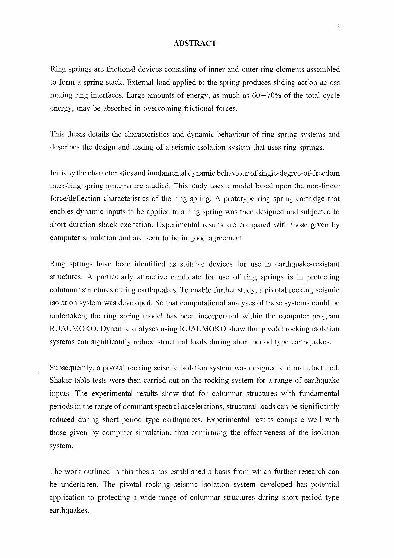
ABSTRACT
Ring springs are frictional devices consisting of inner and outer ring elements assembled
to form a spring stack. External load applied to the spring produces sliding action across
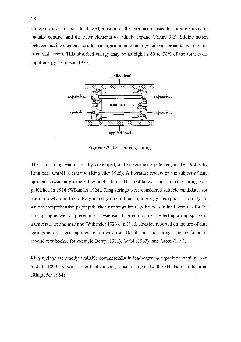
mating ring interfaces. Large amounts of energy, as much as 60-70% of the total cycle
energy, may be absorbed in overcoming frictional forces.
This thesis details the characteristics and dynamic behaviour of ring spring systems and
describes the design and testing of a seismic isolation system that uses ring springs.
Initially the characteristics and fundamental dynamic behaviour of single-degree-of-freedom
mass/ring spring systems are studied. This study uses a model based upon the non-linear
force/deflection characteristics of the ring spring. A prototype ring spring cartridge that
enables dynamic inputs to be applied to a ring spring was then designed and subjected to
short duration shock excitation. Experimental results are compared with those given by
computer simulation and are seen to be in good agreement.
Ring spnngs have been identified as suitable devices for use in earthquake-resistant
structures. A particularly attractive candidate for use of ring springs is in protecting
columnar structures during earthquakes. To enable further study, a pivotal rocking seismic
isolation system was developed. So that computational analyses of these systems could be
undertaken, the ring spring model has been incorporated within the computer program
RUAUMOKO. Dynamic analyses using RUAUMOKO show that pivotal rocking isolation
systems can significantly reduce structural loads during short period type earthquakes.
Subsequently, a pivotal rocking seismic isolation system was designed and manufactured.
Shaker table tests were then carried out on the rocking system for a range of earthquake
inputs. The experimental results show that for colunmar structures with fundamental
periods in the range of dominant spectral accelerations, structural loads can be significantly
reduced during short period type earthquakes. Experimental results· compare well with
those given by computer simulation, thus confirming the effectiveness of the isolation
system.
The work outlined in this thesis has established a basis from which further research can
be undertaken. The pivotal rocking seismic isolation system developed has potential
application to protecting a wide range of columnar structures during short period type
earthquakes.

11
Hill, K.E.
Hill, K.E.
Hill, K.E.
Hill, K.E.
Hill, K.E.
Hill, K.E.
Hill, K.E.
Hill, K.E.
Hill, K.E.
Hill, K.E.
111
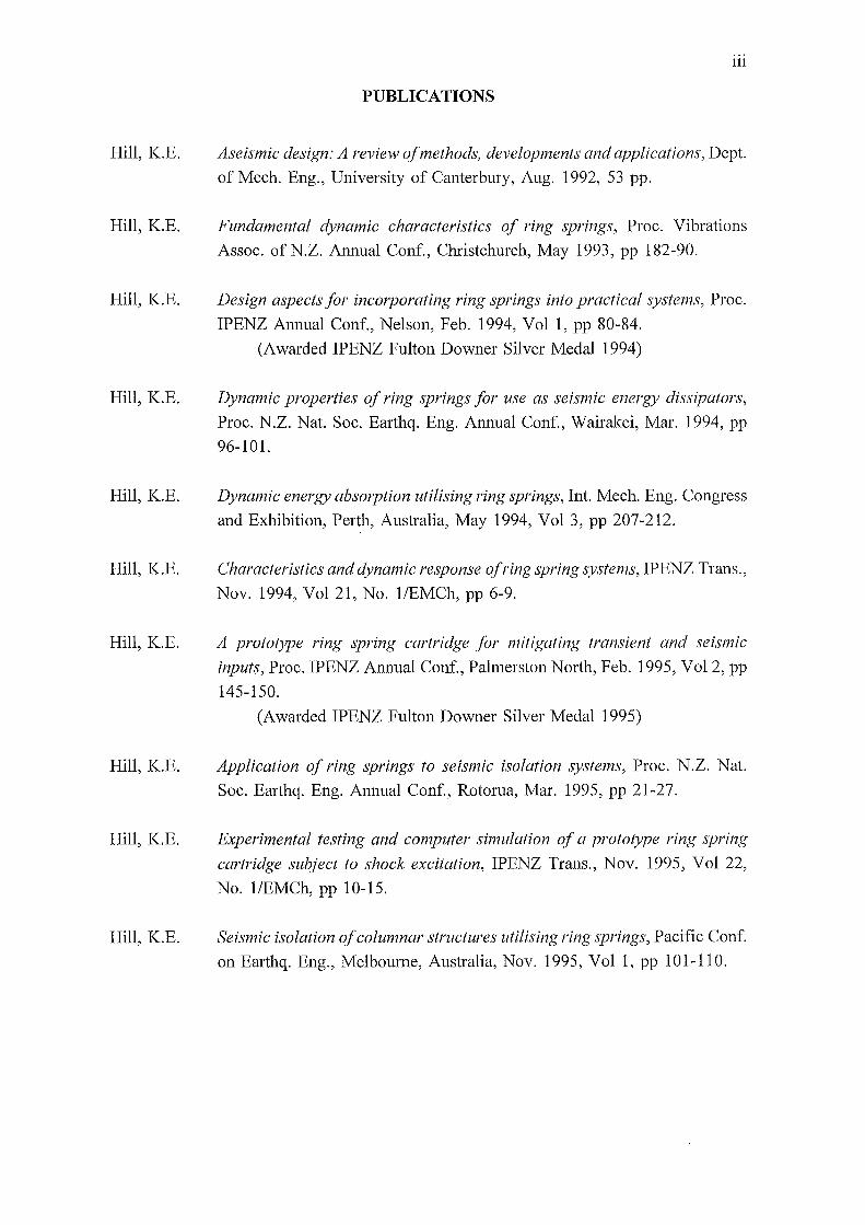
PUBLICATIONS
Aseismic design: A review of methods, developments and applications, Dept.
of Mech. Eng., University of Canterbury, Aug. 1992, 53 pp.
Fundamental dynamic characteristics of ring springs, Proc. Vibrations
Assoc. ofN.Z. Annual Conf., Christchurch, May 1993, pp 182-90.
Design aspects for incmporating ring springs into practical systems, Proc.
IPENZ Almual Conf., Nelson, Feb. 1994, Vol 1, pp 80-84.
(Awarded IPENZ Fulton Downer Silver Medal 1994)
Dynamic properties of ring springs for use as seismic energy dissipators,
Proc. N.Z. Nat. Soc. Earthq. Eng. Annual Conf., Wairakei, Mar. 1994, pp
96-101.
Dynamic energy absorption utilising ring springs, Int. Mech. Eng. Congress
and Exhibition, Perth, Australia, May 1994, Vol 3, pp 207-212.
Characteristics and dynamic response ofring spring systems, IPENZ Trans.,
Nov. 1994, Vol 21, No. 1/EMCh, pp 6-9.
A prototype ring spring cartridge for mitigating transient and seismic
inputs, Proc. IPENZ Annual Conf., Palmerston North, Feb. 1995, Vol 2, pp
145-150.
(Awarded IPENZ Fulton Downer Silver Medal 1995)
Application of ring springs to seismic isolation systems, Proc. N.Z. Nat.
Soc. Earthq. Eng. Annual Conf., Rotorua, Mar. 1995, pp 21-27.
Experimental testing and computer simulation of a prototype ring spring
cartridge subject to shock excitation, IPENZ Trans., Nov. 1995, Vol 22,
No. 1/EMCh, pp 10-15.
Seismic isolation of columnar structures utilising ring springs, Pacific Conf.
on Earthq. Eng., Melbourne, Australia, Nov. 1995, Vol 1, pp 101-110.

lV

v
ACKNOWLEDGEMENTS
I sincerely thank Professor RJ Astley for his supervision of this research project. The
associate supervision of Professor Emeritus LA Erasmus, Drs JS Smaill and AK Ditcher
is gratefully acknowledged. I also thank Dr AJ Carr for his assistance with the
RUAUMOKO computer program.
To the other members of the Mechanical and Civil Engineering Departments who have
assisted during this project, I offer many thanks; of special mention are the workshop staff
of Messrs 0 Bolt, K Brown and CS Amies.
Warm gratitude is giVen to my fellow postgraduates, past and present, for their
encouragement and constructive discussions. Particular thanks to Mr RJ Henderson for his
many valuable comments. The co-operation of the staff of Industrial Research Ltd,
Christchurch, especially that of Mr B Donohue and Dr L Lengoc, is warmly aclmowledged.
I thank the Emihquake Commission and the University Grants Committee, New Zealand,
for providing financial support for this work. Thanks is also given to Ringfeder GmbH,
Germany, for providing the ring springs used in the research programme.

Vl
Vll
TABLE OF CONTENTS
Abstract ..................................................... 1
Publications . . . . . . . . . . . . . . . . . . . . . . . . . . . . . . . . . . . . . . . . . . . . . . . . . . 111
Acknowledgements . . . . . . . . . . . . . . . . . . . . . . . . . . . . . . . . . . . . . . . . . . . . . v
Table of contents . . . . . . . . . . . . . . . . . . . . . . . . . . . . . . . . . . . . . . . . . . . . . vii
Notation ................................................... x1n
1. INTRODUCTION
1.1 General . . . . . . . . . . . . . . . . . . . . . . . . . . . . . . . . . . . . . . . . . . . . . . 1
1.2 Objectives of research . . . . . . . . . . . . . . . . . . . . . . . . . . . . . . . . . . . . 1
1.3 Scope and outline of the thesis . . . . . . . . . . . . . . . . . . . . . . . . . . . . . . 2
2. ASEISMIC DESIGN: METHODS, DEVELOPMENTS AND APPLICATIONS
2.1 Introduction . . . . . . . . . . . . . . . . . . . . . . . . . . . . . . . . . . . . . . . . . . . 5
2.2 Aseismic design methods . . . . . . . . . . . . . . . . . . . . . . . . . . . . . . . . . . 5
2.3 Strength design . . . . . . . . . . . . . . . . . . . . . . . . . . . . . . . . . . . . . . . . . 6
2.3.1 Working stress method . . . . . . . . . . . . . . . . . . . . . . . . . . . . . . . 6
2.3 .2 Strength method . . . . . . . . . . . . . . . . . . . . . . . . . . . . . . . . . . . . 7
2.4 Response control . . . . . . . . . . . . . . . . . . . . . . . . . . . . . . . . . . . . . . . . 8
2.4.1 Passive, active and semi-active control . . . . . . . . . . . . . . . . . . . . 9
(a) Passive control . . . . . . . . . . . . . . . . . . . . . . . . . . . . . . . . . . 9
(b) Active control . . . . . . . . . . . . . . . . . . . . . . . . . . . . . . . . . . 9
(c) Semi-active control . . . . . . . . . . . . . . . . . . . . . . . . . . . . . . 11
2.5 Response control methods . . . . . . . . . . . . . . . . . . . . . . . . . . . . . . . . 12
2.5.1 Seismic isolation . . . . . . . . . . . . . . . . . . . . . . . . . . . . . . . . . . 12
(a) Characteristics of seismic isolation systems . . . . . . . . . . . . . . 12
(b) System flexibility . . . . . . . . . . . . . . . . . . . . . . . . . . . . . . . 13
(c) Dissipative mechanisms . . . . . . . . . . . . . . . . . . . . . . . . . . . 14
(d) Advantages of seismic isolation . . . . . . . . . . . . . . . . . . . . . . 19
(e) Seismic isolation applications in New Zealand . . . . . . . . . . . . 19
2.5.2 Supplemental damping . . . . . . . . . . . . . . . . . . . . . . . . . . . . . . 21
(a) Auxiliary mass dampers . . . . . . . . . . . . . . . . . . . . . . . . . . . 21
(b) Mechanical dissipators . . . . . . . . . . . . . . . . . . . . . . . . . . . . 22
(c) Advantages of supplemental damping . . . . . . . . . . . . . . . . . . 24
2.5.3 Structural parameter adjustment . . . . . . . . . . . . . . . . . . . . . . . . 25
2.6 Sumn1ary . . . . . . . . . . . . . . . . . . . . . . . . . . . . . . . . . . . . . . . . . . . . 25
vm
3. RING SPRINGS: CHARACTERISTICS AND DESIGN REQUIREMENTS
3.1 Introduction . . . . . . . . . . . . . . . . . . . . . . . . . . . . . . . . . . . . . . . . . . 27
3.2 Ring springs . . . . . . . . . . . . . . . . . . . . . . . . . . . . . . . . . . . . . . . . . . 27
3.2.1 Description and literature review . . . . . . . . . . . . . . . . . . . . . . . 27
3.2.2 Ring spring stiffness equations . . . . . . . . . . . . . . . . . . . . . . . . . 30
3.2.3 Ring spring hysteresis diagram . . . . . . . . . . . . . . . . . . . . . . . . . 30
3.3 Design requirements for practical use of ring springs . . . . . . . . . . . . . . 31
3.3.1 Ring spring lubrication . . . . . . . . . . . . . . . . . . . . . . . . . . . . . . 31
3.3.2 Housing and guidance of ring springs . . . . . . . . . . . . . . . . . . . . 32
3.3.3 Spring pre-displacement . . . . . . . . . . . . . . . . . . . . . . . . . . . . . 32
3.3.4 Energy absorption and temperature limits . . . . . . . . . . . . . . . . . 32
3.4 Ring spring configurations . . . . . . . . . . . . . . . . . . . . . . . . . . . . . . . . 35
3.4.1 Bi-directional ring spring systems . . . . . . . . . . . . . . . . . . . . . . . 35
3.4.2 Force/deflection characteristics . . . . . . . . . . . . . . . . . . . . . . . . . 36
3.5 Free vibration response of bi-directional mass/ring spring systems . . . . . 36
3.5.1 System model . . . . . . . . . . . . . . . . . . . . . . . . . . . . . . . . . . . . 36
3.5.2 Governing equation of motion . . . . . . . . . . . . . . . . . . . . . . . . . 37
3.5.3 Dynamic response . . . . . . . . . . . . . . . . . . . . . . . . . . . . . . . . . 38
(a) Displacement solution . . . . . . . . . . . . . . . . . . . . . . . . . . . . 38
(b) Acceleration solution . . . . . . . . . . . . . . . . . . . . . . . . . . . . . 39
3. 5.4 Ring spring damping factor . . . . . . . . . . . . . . . . . . . . . . . . . . . 40
3.6 Summary . . . . . . . . . . . . . . . . . . . . . . . . . . . . . . . . . . . . . . . . . . . . 41
4. HYSTERESIS CHARACTERISTICS OF A BI-DIRECTIONAL RING SPRING
CARTRIDGE ASSEMBLY
4.1 Introduction . . . . . . . . . . . . . . . . . . . . . . . . . . . . . . . . . . . . . . . . . . 43
4.2 Ring spring selection and quasi-static test results . . . . . . . . . . . . . . . . . 43
4.2.1 Physical properties of the selected ring spring . . . . . . . . . . . . . . 44
4.2.2 Quasi-static hysteresis diagram . . . . . . . . . . . . . . . . . . . . . . . . . 44
4.2.3 Force/deflection stiffnesses . . . . . . . . . . . . . . . . . . . . . . . . . . . 45
4.3 Theoretical hysteresis characteristics of bi-directional ring
spring systems . . . . . . . . . . . . . . . . . . . . . . . . . . . . . . . . . . . . . . . . 46
4.3 .1 Force/deflection stiffnesses . . . . . . . . . . . . . . . . . . . . . . . . . . . 46
(a) Zero pre-displacement systems . . . . . . . . . . . . . . . . . . . . . . 47
(b) Pre-displaced systems . . . . . . . . . . . . . . . . . . . . . . . . . . . . 48
4.4 A prototype bi-directional ring spring cartridge . . . . . . . . . . . . . . . . . . 49
lX
4.4.1 Design detail . . . . . . . . . . . . . . . . . . . . . . . . . . . . . . . . . . . . . 50
4.4.2 Manufactured ring spring cartridge . . . . . . . . . . . . . . . . . . . . . . 50
4.5 Experimental testing of the ring spring cartridge . . . . . . . . . . . . . . . . . 51
4.5.1 Test facility . . . . . . . . . . . . . . . . . . . . . . . . . . . . . . . . . . . . . . 51
4.5.2 Quasi-static hysteresis diagrams . . . . . . . . . . . . . . . . . . . . . . . . 52
(a) 16% pre-displacement . . . . . . . . . . . . . . . . . . . . . . . . . . . . 52
(b) 28% pre-displacement . . . . . . . . . . . . . . . . . . . . . . . . . . . . 53
(c) Force/ deflection stiffnesses . . . . . . . . . . . . . . . . . . . . . . . . . 53
4.6 Summary . . . . . . . . . . . . . . . . . . . . . . . . . . . . . . . . . . . . . . . . . . . . 54
5. FREE VIBRATION BEHAVIOUR OF PRE-DISPLACED AND PRE-LOADED
MASS/RING SPRING SYSTEMS
5 .1 Introduction . . . . . . . . . . . . . . . . . . . . . . . . . . . . . . . . . . . . . . . . . . 55
5.2 Computer modelling of SDOF mass/ring spring systems . . . . . . . . . . . . 55
5.2.1 Numerical integration method . . . . . . . . . . . . . . . . . . . . . . . . . 55
5.2.2 Ring spring model computer algorithm . . . . . . . . . . . . . . . . . . . 56
5.2.3 Types of ring spring systems considered in the study . . . . . . . . . . 56
5.3 Free vibration behaviour of pre-displaced ring spring systems . . . . . . . . 56
5.3.1 System model . . . . . . . . . . . . . . . . . . . . . . . . . . . . . . . . . . . . 56
5.3.2 Force/deflection characteristics . . . . . . . . . . . . . . . . . . . . . . . . . 57
5.3.3 Equation of motion . . . . . . . . . . . . . . . . . . . . . . . . . . . . . . . . 59
5.3.4 Dynamic response . . . . . . . . . . . . . . . . . . . . . . . . . . . . . . . . . 59
5.4 Free vibration behaviour of pre-loaded ring spring systems . . . . . . . . . . 62
5.4.1 System model . . . . . . . . . . . . . . . . . . . . . . . . . . . . . . . . . . . . 62
5.4.2 Force/deflection characteristics . . . . . . . . . . . . . . . . . . . . . . . . . 63
5.4.3 Equation of motion . . . . . . . . . . . . . . . . . . . . . . . . . . . . . . . . 64
5.4.4 Dynamic response . . . . . . . . . . . . . . . . . . . . . . . . . . . . . . . . . 64
5.5 Free vibration behaviour of pre-displaced pre-loaded ring spring systems 68
5.5.1 System model . . . . . . . . . . . . . . . . . . . . . . . . . . . . . . . . . . . . 68
5.5.2 Force/deflection characteristics . . . . . . . . . . . . . . . . . . . . . . . . . 68
5.5.3 Equation of motion . . . . . . . . . . . . . . . . . . . . . . . . . . . . . . . . 69
5.5.4 Dynamic response . . . . . . . . . . . . . . . . . . . . . . . . . . . . . . . . . 69
5.6 Sumn1ary . . . . . . . . . . . . . . . . . . . . . . . . . . . . . . . . . . . . . . . . . . . . 72
X
6. DYNAMIC TESTING OF A PRE-DISPLACED MASS/RING SPRING
CARTRIDGE SYSTEM: COMPARISON WITH COMPUTER SIMULATION
RESULTS
6.1 Introduction . . . . . . . . . . . . . . . . . . . . . . . . . . . . . . . . . . . . . . . . . . 73
6.2 Experimental system . . . . . . . . . . . . . . . . . . . . . . . . . . . . . . . . . . . . 73
6.2.1 Mass/ring spring cartridge system . . . . . . . . . . . . . . . . . . . . . . . 73
6.2.2 Experimental test facility . . . . . . . . . . . . . . . . . . . . . . . . . . . . . 74
6.2.3 Instrumentation . . . . . . . . . . . . . . . . . . . . . . . . . . . . . . . . . . . 75
(a) Accelerometers . . . . . . . . . . . . . . . . . . . . . . . . . . . . . . . . . 7 5
(b) Displacement transducer . . . . . . . . . . . . . . . . . . . . . . . . . . . 76
6.2.4 Data acquisition system . . . . . . . . . . . . . . . . . . . . . . . . . . . . . . 76
6.3 Computational modelling ......................... ·. . . . . . . . 76
6.3.1 Computer model for mass/ring spring system . . . . . . . . . . . . . . . 76
6.3.2 Ring spring cartridge stiffnesses . . . . . . . . . . . . . . . . . . . . . . . . 77
6.4 Experimental tests and computer simulation results . . . . . . . . . . . . . . . 77
6.4.1 Dynamic inputs . . . . . . . . . . . . . . . . . . . . . . . . . . . . . . . . . . . 77
6.4.2 Dynamic response of system subjected to 1 second input . . . . . . . 78
(a) 16% pre-displacement . . . . . . . . . . . . . . . . . . . . . . . . . . . . 78
(b) 28% pre-displacement . . . . . . . . . . . . . . . . . . . . . . . . . . . . 80
6.4.3 Dynamic response of system subjected to 4 second input . . . . . . . 82
(a) 16% pre-displacement . . . . . . . . . . . . . . . . . . . . . . . . . . . . 82
(b) 28% pre-displacement . . . . . . . . . . . . . . . . . . . . . . . . . . . . 84
6.4.4 Discussion of results . . . . . . . . . . . . . . . . . . . . . . . . . . . . . . . . 86
6.5 Summary . . . . . . . . . . . . . . . . . . . . . . . . . . . . . . . . . . . . . . . . . . . . 87
7. EARTHQUAKE-RESISTANT DESIGN UTILISING RING SPRINGS
7.1 Introduction . . . . . . . . . . . . . . . . . . . . . . . . . . . . . . . . . . . . . . . . . . 89
7.2 Emihquake-resistant design . . . . . . . . . . . . . . . . . . . . . . . . . . . . . . . . 89
7.2.1 Seismic isolation systems utilising ring springs . . . . . . . . . . . . . . 89
7.2.2 Potential benefits of ring springs . . . . . . . . . . . . . . . . . . . . . . . 91
7.2.3 Practical applications for use of ring springs . . . . . . . . . . . . . . . 91
7.3 A pivotal rocking seismic isolation system incorporating ring springs . . . 93
7.3.1 Detail of system . . . . . . . . . . . . . . . . . . . . . . . . . . . . . . . . . . . 93
7.3.2 Fundamental period of system . . . . . . . . . . . . . . . . . . . . . . . . . 94
7.4 Computer modelling of PRSIS's . . . . . . . . . . . . . . . . . . . . . . . . . . . . 95
7.4.1 Generalised equation of motion . . . . . . . . . . . . . . . . . . . . . . . . 95
XI
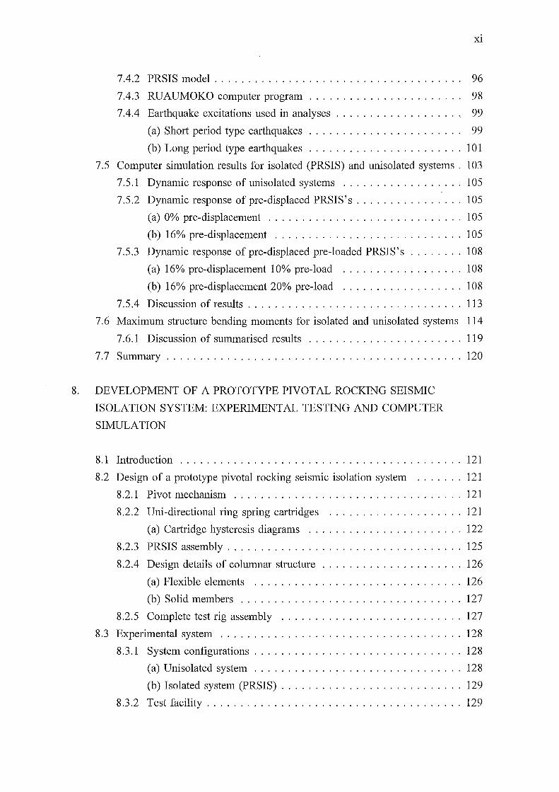
7.4.2 PRSIS model . . . . . . . . . . . . . . . . . . . . . . . . . . . . . . . . . . . . . 96
7.4.3 RUAUMOKO computer program . . . . . . . . . . . . . . . . . . . . . . . 98
7.4.4 Earthquake excitations used in analyses . . . . . . . . . . . . . . . . . . . 99
(a) Short period type earthquakes . . . . . . . . . . . . . . . . . . . . . . . 99
(b) Long period type earthquakes . . . . . . . . . . . . . . . . . . . . . . . 1 0 1
7.5 Computer simulation results for isolated (PRSIS) and unisolated systems . 103
7.5.1 Dynamic response of unisolated systems .................. 105
7.5.2 Dynamic response of pre-displaced PRSIS's ................ 105
(a) 0% pre-displacement ............................. 105
(b) 16% pre-displacement . . . . . . . . . . . . . . . . . . . . . . . . . . . . 105
7.5.3 Dynamic response of pre-displaced pre-loaded PRSIS's ........ 108
(a) 16% pre-displacement 10% pre-load .................. 108
(b) 16% pre-displacement 20% pre-load .................. 108
7. 5 .4 Discussion of results . . . . . . . . . . . . . . . . . . . . . . . . . . . . . . . . 113
7.6 Maximum structure bending moments for isolated and unisolated systems 114
7.6.1 Discussion of summarised results ....................... 119
7.7 Summary ............................................ 120
8. DEVELOPMENT OF A PROTOTYPE PIVOTAL ROCKING SEISMIC
ISOLATION SYSTEM: EXPERIMENTAL TESTING AND COMPUTER
SIMULATION
8.1 Introduction 121
8.2 Design of a prototype pivotal rocking seismic isolation system ....... 121
8.2.1 Pivot mechanism .................................. 121
8.2.2 Uni-directional ring spring cartridges .................... 121
(a) Cartridge hysteresis diagrams ....................... 122
8.2.3 PRSIS assembly ................................... 125
8.2.4 Design details of columnar structure ..................... 126
(a) Flexible elements ............................... 126
(b) Solid members ................................. 127
8.2.5 Complete test rig assembly ........................... 127
8.3 Experimental system .................................... 128
8.3.1 System configurations ............................... 128
(a) Unisolated system ............................... 128
(b) Isolated system (PRSIS) ........................... 129
8.3.2 Test facility ...................................... 129
Xll
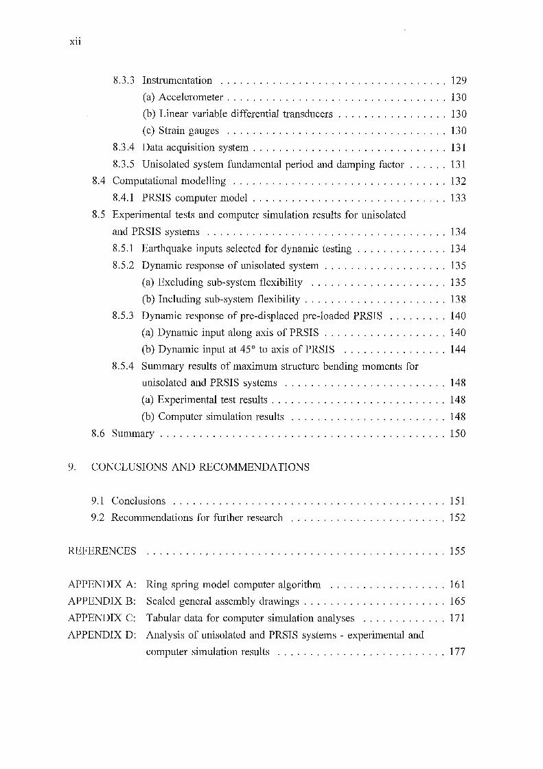
8.3.3 Instrumentation ................................... 129
(a) Accelerometer .................................. 130
(b) Linear variable differential transducers ................. 130
(c) Strain gauges . . . . . . . . . . . . . . . . . . . . . . . . . . . . . . . . . . 130
8.3 .4 Data acquisition system . . . . . . . . . . . . . . . . . . . . . . . . . . . . . . 131
8.3.5 Unisolated system fundamental period and damping factor ...... 131
8.4 Computational modelling ................................. 132
8.4.1 PRSIS computer model .............................. 133
8.5 Experimental tests and computer simulation results for unisolated
and PRSIS systems ..................................... 134
8. 5.1 Earthquake inputs selected for dynamic testing . . . . . . . . . . . . . . 134
8.5.2 Dynamic response of unisolated system ................... 135
(a) Excluding sub-system flexibility . . . . . . . . . . . . . . . . . . . . . 13 5
(b) Including sub-system flexibility . . . . . . . . . . . . . . . . . . . . . . 13 8
8.5.3 Dynamic response of pre-displaced pre-loaded PRSIS ......... 140
(a) Dynamic input along axis of PRSIS . . . . . . . . . . . . . . . . . . . 140
(b) Dynamic input at 45° to axis of PRSIS ................ 144
8.5.4 Summary results of maximum structure bending moments for
unisolated and PRSIS systems . . . . . . . . . . . . . . . . . . . . . . . . . 148
(a) Experimental test results . . . . . . . . . . . . . . . . . . . . . . . . . . . 148
(b) Computer simulation results . . . . . . . . . . . . . . . . . . . . . . . . 148
8.6 Summary ............................................ 150
9. CONCLUSIONS AND RECOMMENDATIONS
9.1 Conclusions . . . . . . . . . . . . . . . . . . . . . . . . . . . . . . . . . . . . . . . . . . 151
9.2 Recommendations for further research . . . . . . . . . . . . . . . . . . . . . . . . 152
REFERENCES ............................................... 155
APPENDIX A: Ring spring model computer algorithm .................. 161
APPENDIX B: Scaled general assembly drawings ...................... 165
APPENDIX C: Tabular data for computer simulation analyses ............. 171
APPENDIX D: Analysis of unisolated and PRSIS systems - experimental and
computer simulation results . . . . . . . . . . . . . . . . . . . . . . . . . . 1 77

xm
NOTATION
a rocking arm radius
Ai inner element cross sectional area
A0 outer element cross sectional area
b height to centre of gravity of column
[ C] damping matrix
Ed energy absorbed for decreasing load
Ei energy absorbed for increasing load
E modulus of elasticity
F ~-tN, frictional force
F 0 Ki /1, force at transition from Ko to Ki
g gravity
10 IG+mb2 = ( 4mb2)/3, mass moment of inertia about point 0
IG mass moment of inertia about centre of gravity
k spring stiffness
k* either stiffness K0, Ki, K1, or Kd
Ko ring spring stiffness at origin
K1 ring spring stiffness between Ki and Kd
Kd decreasing ring spring stiffness
Ke elastic spring stiffness
Kerr effective spring stiffness (secant stiffness)
Ki increasing ring spring stiffness
[K] stiffness matrix
m mass
[M] mass matrix
N total normal force
n total number of interfaces of ring spring
p{t} time varying load
P d decreasing compressive load
Pi increasing compressive load
ri inner ring element mean radius
rm (ri+ro)/2, mean radius
r0
outer ring element mean radius
{r} influence coefficient vector
T1 cycle 1/4 period on stiffness Kd
T2 cycle 114 period on stiffness Ki

XIV
T,is first mode period of isolated system
T 1unis first mode period of unisolated system
Tn period
t total time
ua mg/Ki, initial displacement due to load mg
u displacement of mass
ii acceleration of mass
{ v} total displacement vector
{ v} total velocity vector
{ v} total acceleration vector
w relative displacement
w relative acceleration
{ w} relative displacement vector
{ w} relative velocity vector
{ w} relative acceleration vector
W mg, weight
xg ground displacement
xg ground acceleration
z input displacement
z input acceleration
a ring spring taper angle
y cycle decay factor
8 deflection of ring spring
11 ring spring pre-displacement
11 1 initial spring displacement
11i spring displacement after i cycles
11i+q spring displacement after i+q cycles
s damping factor
8 angular rotation
8 angular acceleration
).l coefficient of friction
wnd natural frequency on stiffness Kd
wni natural frequency on stiffness Ki
1
Chapter 1
INTRODUCTION
1.1 GENERAL
Earthquakes plague many regions of the world resulting in significant damage and loss of
life each year. Damage caused by several seconds of violent ground shaking can be
devastating to communities and countries alike. The destruction earthquakes can cause has
been graphically demonstrated in recent years. In 1994 in Northridge, USA, an earthquake
of moment magnitude 6.7, killed 57 people and caused damage estimated at US$18-20
billion (Norton et al. 1994). More recently, in 1995 in Kobe, Japan, approximately 5500
people lost their lives in an earthquake of Richter magnitude 7 .2. The direct rebuilding cost
as a result of this earthquake has been estimated at approximately NZ$200 billion (Park
et al. 1995).
In today' s society of increasingly advanced technology - taller structures, nuclear power
generation, increased reliance on lifeline utilities such as water supply and electricity, it is
imperative that the nature of earthquakes, and their effect on structures, be understood.
This has lead to a vast amount of work being undertaken in the field of earthquake
engineering and is evidenced by an enormous amount of published literature. The general
aim of such work is to enable a greater understanding of earthquakes and their influence
on man-made structures, thus prevent loss of life and minimise damage and economic loss.
1.2 OBJECTIVES OF RESEARCH
The initial objective of this study was to examme the vanous earthquake-resistant
(aseismic) design methods used to protect structures and structural systems during
earthquakes. This is detailed in Chapter 2.
Based on knowledge of these ase1sm1c design methods, the second objective was to
investigate the possibility of utilising a frictional device known as a ring spring in
earthquake-resistant structures.
2
1.3 SCOPE AND OUTLINE OF THE THESIS
The following outline describes the scope of the research reported in this thesis. First, the
methods and principles utilised in aseismic design are detailed in Chapter 2. Of the
methods presented, special discussion is given to that of seismic isolation, a technique that
aims to reduce the level of loading experienced by a structure during an earthquake. This
is achieved by isolating the structure from the ground motion.
Chapter 3 details the basic characteristics of ring springs. The equations that define the ring
spring stiffness characteristics are detailed; these equations form the basis of a model for
the ring spring. Design requirements for utilising ring springs in practical applications are
then discussed. Subsequently, different types of ring spring configurations are detailed and
solutions to the equations of motion for a bi-directional ring spring system are presented.
A prototype ring spring cartridge that allows bi-directional dynamic inputs to be applied
to ring springs was designed and manufactured. Chapter 4 details the hysteresis
characteristics obtained from experimental tests conducted on the cartridge.
Utilising these hysteresis characteristics, Chapter 5 then details computer simulation
analyses that predict the dynamic behaviour of single-degree-of-freedom (SDOF) mass/ring
spring systems. The study considers the effect of applying a pre-displacement and a pre
load to the ring spring.
To assess the accuracy of computer simulation results, experimental tests were undertaken.
Chapter 6 details experimental testing of a mass/ring spring cartridge system. Testing is
carried out on a single-axis shaker table facility and experimental results are determined
for various pre-displacements and dynamic inputs. These results are then compared with
those given by computer simulation.
The possibility of utilising ring springs in earthquake-resistant applications is examined in
Chapter 7. Discussion considers possible situations identified as suitable for use of ring
springs. Of these, seismic isolation systems are seen as offering considerable potential. To
explore this option, a pivotal rocking seismic isolation system has been developed. Details
of this system, as well as results of computer simulation analyses, are presented. To

3
facilitate this modelling, the ring spring model has been incorporated within the computer
program RUAUMOKO.
Chapter 8 details experimental testing of the pivotal rocking seismic isolation system
subject to four different short period type earthquakes. Test results are then compared with
those given by computer simulation.
Conclusions and recommendations for future research are reported in Chapter 9.

4

Chapter 2
ASEISMIC DESIGN: METHODS, DEVELOPMENTS
AND APPLICATIONS
2.1 INTRODUCTION
5
In the design of structures situated in regions of seismic risk, it is necessary that an
appropriate earthquake-resistant (aseismic) design technique be employed. This is to
minimise the likelihood of loss of life and the collapse of structures during a major
earthquake. This chapter examines the various methods used in aseismic design. Discussion
covers numerous developments and considers their practical application.
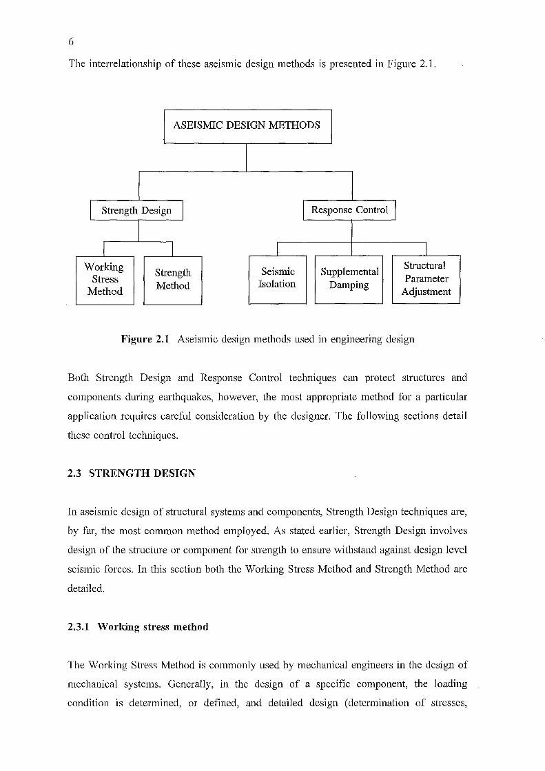
2.2 ASEISMIC DESIGN METHODS
The aseismic design methods utilised in engineering design can be broadly classified into
two principal techniques:
(a) Strength Design: With this technique the structure is designed for strength to
ensure it can withstand design level forces. Two procedures are commonly
employed in this design approach; these are:
• Working Stress Method - primarily an elastic design approach.
• Strength Method - primarily an inelastic design approach.
(b) Response Control: In this technique the response of a structure is regulated by
incorporating specific devices within the system. The following three procedures
may be utilised:
• Seismic Isolation - isolation of the structure from ground disturbances.
• Supplemental Damping - controlling structural response through
increased damping.
• Structural Parameter Adjustment - incorporating within the structural
system actively controlled members.
6
The interrelationship of these aseismic design methods is presented in Figure 2.1.
ASEISMIC DESIGN METHODS
I Strength Design I I Response Control I
I I I I Working Strength Seismic Supplemental
Structural Stress
Method Isolation Damping Parameter
Method Adjustment
Figure 2.1 Aseismic design methods used in engineering design
Both Strength Design and Response Control techniques can protect structures and
components during earthquakes, however, the most appropriate method for a particular
application requires careful consideration by the designer. The following sections detail
these control techniques.
2.3 STRENGTH DESIGN
In aseismic design of structural systems and components, Strength Design techniques are,
by far, the most common method employed. As stated earlier, Strength Design involves
design of the structure or component for strength to ensure withstand against design level
seismic forces. In this section both the Working Stress Method and Strength Method are
detailed.
2.3.1 Worl{ing stress method
The Working Stress Method is commonly used by mechanical engineers in the design of
mechanical systems. Generally, in the design of a specific component, the loading
condition is determined, or defined, and detailed design (determination of stresses,
7
deflections etc.) is based upon this assigned load. The basis of the Working Stress Method
is that under working loads, an allowable working stress should not be exceeded. This
allowable working stress is usually determined by dividing the yield stress by a design
factor.
Generally, structures such as buildings are designed using relatively low seismic factors;
their earthquake resistance dependent on post yield ductility. However, for many items of
electrical and mechanical equipment, deformation due to yielding of fixings would impair
the operation of the equipment, hence, it is generally more appropriate to secure equipment
to withstand elastically the earthquake design level forces. Nevertheless, it remains of
foremost importance in the design of such plant and equipment that the overall ductility
of the component fixings should be considered to avoid sudden failure in the event of the
design earthquake load being exceeded. This point is sometimes overlooked by mechanical
engineers in the design of equipment fixings required to withstand earthquake induced
loads.
2.3.2 Strength method
The Strength Method is generally used by civil engineers in structural design. In this
method working loads are multiplied by appropriate factors, usually specified in design
codes; structural members are then proportioned based upon their ultimate strength -
usually concrete at maximum strength and steel at yield. Bridges and buildings are typical
structures that are designed using the Strength Method approach.
In structural design, it is generally accepted that it is uneconomic to design a building to
remain elastic during the greatest likely earthquake (Park 1987). Thus, the Strength Method
employs an inelastic design philosophy. This ensures adequate structural ductility by
utilising the principles of capacity design whereby chosen inelastic mechanisms provide
both adequate strength and ductility. To ensure yielding occurs within these plastic hinges,
other structural elements are provided with increased strength. In conventional buildings
these ductile yielding mechanisms are concentrated in beams at beam-column connections.
The purpose of incorporating these mechanisms within the system is to allow a
considerable amount of the energy associated with the seismic disturbance to be absorbed
by the structure itself.

8
In applying the Strength Method, the designer is able to assess the ductility of the structure
in the post-elastic range; the designed collapse mechanisms enable an appreciation of the
likely structural response during an earthquake. This fact is not readily appreciated in
applying the Working Stress Method.
Engineers, in applying Strength Design techniques in the design of structural systems, are
usually required to comply with statutory codes and standards. In New Zealand codes,
commonly both the Strength Method and Working Stress Method may be appropriate
design methods, except where specifically stated. However, for reasons outlined earlier,
clear preference is given to employing the Strength Method. This is emphasised by terming
the Working Stress Method the Alternative Method.
The general design philosophy that embodies building codes employing the Strength
Method can be summarised as follows: In the event of a major earthquake, significant
structural damage may result, however, complete collapse of the structure should be
prevented; in the event of a severe earthquake that can be expected during the life of the
building, the aim is for minimal or no damage (Park 1987).
In applying the Strength Design approach, the mechanism that provides structural
protection is the ability of the structure to resist elastically, or absorb inelastically, the input
energy it experiences during a seismic disturbance. A means of enhancing seismic
resistance is by controlling structural response, i.e., reducing seismic energy transmitted
into the structure. This method, Response Control, is presented in the next section.
2.4 RESPONSE CONTROL
Response Control is an aseismic design approach that involves regulating the response of
a structure during a seismic disturbance. This approach utilises any of the following
methods: Seismic Isolation, Supplemental Damping, or Structural Parameter Adjustment.
In the discussion that follows, the devices these methods employ are described.

9
2.4.1 Passive, active and semi-active control
Response Control techniques may use passive, active or semi-active control.
(a) Passive control
In passive control, passive devices are embodied within the structural system. Passive
devices require no power supply; they respond directly to the seismic disturbance and
exhibit response characteristics dependent on their physical properties. These devices can
either store or dissipate the energy associated with a seismic disturbance. Examples of
passive devices for protecting engineering systems from earthquake damage include: lead
rubber bearings, lead extrusion dampers, mild steel energy dissipators, elastic springs,
viscous dampers, visco-elastic dampers, and frictional dissipators (Hill 1992, Skinner et al.
1993). Passive devices offer advantages that they are generally inexpensive, reliable and
possess well defined characteristics.
(b) Active control
In active control, active devices apply control forces at specific locations throughout the
structure. These control forces counteract the seismic response of the structure, thereby
reducing the forces experienced by structural elements.
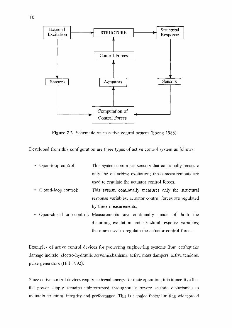
Figure 2.2 presents the basic configuration of an active control system (Soong 1988); the
components comprise:
( 1) Sensors appropriately positioned within the structure to measure either, the disturbing
excitation, structural response variables, or both;
(2) A control unit to register the sensor inputs and compute the required control forces
based on a prescribed control algorithm;
(3) Actuators that apply the required control forces.
10
External Structural I STRUCTURE I .. Excitation I
~
Response A
I Control Forces
A
r , I Sensors I I J\ctuators I I Sensors I
Computation of .. ~
Control Forces ~
Figure 2.2 Schematic of an active control system (Soong 1988)
Developed from this configuration are three types of active control system as follows:
• Open-loop control:
• Closed-loop control:
This system comprises sensors that continually measure
only the disturbing excitation; these measurements are
used to regulate the actuator control forces.
This system continually measures only the structural
response variables; actuator control forces are regulated
by these measurements.
• Open-closed loop control: Measurements are continually made of both the
disturbing excitation and structural response variables;
these are used to regulate the actuator control forces.
Examples of active control devices for protecting engineering systems from earthquake
damage include: electro-hydraulic servomechanisms, active mass dampers, active tendons,
pulse generators (Hill 1992).
Since active control devices require external energy for their operation, it is imperative that
the power supply remains uninterrupted throughout a severe seismic disturbance to
maintain structural integrity and performance. This is a major factor limiting widespread
11
use of active control in protecting engineering systems from earthquake damage. Other
disadvantageous features include maintenance requirements as well as the large power
requirement. Generally active control systems are more costly and less reliable (due to their
complexity) than passive control systems.
Despite these shortcomings, active control has been applied in a number of practical
applications to reduce wind-induced vibrations in buildings. For example, a 400-ton
auxiliary mass damper is installed on the 59th floor of the Citicorp Building in New York
City; the damper controls the first mode bending response of the building (Miller et al.
1988).
(c) Semi -active control
Semi-active control is a control method that combines the characteristics of both passive
and active control. In this type of control the structural parameters of the system: mass,
stiffness and damping, are modified or adjusted (usually using control actuators) rather than
directly applying control forces to counteract the seismic response of the structure (as in
active control). Thus, the supply energy requirement of semi-active control systems is
generally considerably less than that of active control systems.
As an example of a semi-active control device, Karnopp et al. (1974) discuss a system that
incorporates a conventional passive damper whose force across the device is controllable.
An example of this type of device is a damper with a variable damping coefficient. It is
reported that semi-active control systems can provide many of the performance gains of
active systems. These include: improved vibrational control by providing adjustable
parameters to suit varying excitation or response characteristics; simpler and less costly
hardware than active control systems since semi-active systems require only signal
processing and low level power supplies.
Hrovat et al. (1983) compared the performance of a semi-active tuned mass damper (TMD)
with both passive and active TMD's; they found that semi-active TMD's offered significant
improvements over passive TMD's for reducing wind-induced vibrations in buildings.
Furthermore, the performance of a semi-active TMD was shown to be comparable with a
fully active TMD.
12
2.5 RESPONSE CONTROL METHODS
This section details the characteristics of the Response Control techniques: Seismic
Isolation, Supplemental Damping, and Structural Parameter Adjustment.
2.5.1 Seismic isolation
Seismic Isolation is a Response Control technique that aims to protect structures during
earthquakes. This is essentially achieved by isolating the structure from the ground
disturbance. For over a century, efforts have been made to develop systems that minimise
structural damage during earthquakes. Izumi (1988) describes in a review paper what may
be the first Seismic Isolation system developed. The design consists of supporting a
structure on layers of logs, each layer positioned orthogonally. However, it was not until
1909 that an earthquake-resistant design was patented; this design proposed separating a
building from its foundation by a layer of talc (Kelly 1986).
In the past, Seismic Isolation had been resisted by the engineering profession with favour
given to firmly attaching a structure to its foundations. However, in recent times,
particularly over the last twenty five years, a vast amount of research has been undertaken
in the field of Seismic Isolation with some significant advantages over conventional design
identified. This has resulted in the development and implementation of numerous systems
worldwide. Comprehensive coverage of the history of Seismic Isolation, its development
and practical application, is detailed by Lee and Medland (1978), Kelly (1986), Izumi
(1988), Tajirian and Kelly (1989), Buckle and Mayes (1990), and Skinner et al (1993).
The following sections discuss aspects of Seismic Isolation systems and detail a number
of applications employing various devices.
(a) Characteristics of seismic isolation systems
Principally, a Seismic Isolation system incorporates a mechanism that introduces both
flexibility and damping into a structural system (characteristically at the base attachment,
hence sometimes referred to as Base Isolation). Flexibility is incorporated within the
system to lengthen its fundamental period. This action shifts the fundamental period of the
13
system away from the dominant earthquake energy region, thus significantly reducing the
inertia forces induced in the structure. Damping devices are also incorporated within the
system; their purpose being to dissipate earthquake energy and resist excessive horizontal
displacements at the base of the structure.
Although Seismic Isolation systems may be either passively, actively or semi-actively
controlled, few known applications employ active or semi-active control. Passive control
on the other hand, has been widely used in practice and the following discussion is
confined to this method.
Generally a passive Seismic Isolation system comprises supporting elements and dissipative
mechanisms. The former characterises system flexibility, and the latter provides system
damping.
(b) System flexibility
Several types of supporting elements capable of introducing flexibility into a structural
system include: elastomeric bearings, rollers, sliding plates, cable suspensions, sleeved
piles, rocking/stepping foundations, air cushions and elastic springs (Hill 1992; Skinner et
al. 1993).
An example of a Seismic Isolation system incorporating flexible supports is electrical
power transmission equipment mounted on conventional helical springs (Rani and Kumar
1980). In this system, increased flexibility aims to reduce the induced accelerations in both
the vertical and the horizontal directions. However, the system does not incorporate
additional damping, and so is reliant solely on hysteretic damping within the structure. This
condition could lead to excessive relative displacements.
Laminated rubber-steel bearings have also been used to provide system flexibility. Delfosse
(1977) developed a system, named GAPEC, that utilises these flexible elements. The
system has been applied to the isolation of a 230 kV circuit breaker situated in California
(Delfosse 1980). Delfosse reported that for this system the fundamental period was
increased from 0.4 sec. (without isolators) to 1.37 sec. (with isolators).
14
Other types of supporting elements that have been explored as a means of introducing
system flexibility include roller bearings and ball bearings. Kelly (1986) describes a seven
storey reinforced concrete building built on spherical bearings. Caspe (1984) proposed
supporting an entire building on stainless steel ball bearing clusters and use
polytetrafluoroethylene (PTFE) control pads to provide a minimum force to resist service
loads.
(c) Dissipative mechanisms
Practical Seismic Isolation systems also require dissipative elements that absorb the seismic
input energy and limit excessive base deflections. These elements can be classified into the
following three categories: hysteretic dampers, viscous dampers, and friction dampers.
(i) Hysteretic Damping
Hysteretic dampers provide damping by utilising the deformation properties of materials,
such as, steel and lead; these dampers generally exhibit displacement-dependent
characteristics. Extensive research has been undertaken in New Zealand on the use of steel
as a hysteretic damping material. This has resulted in the development of various types of
mild steel hysteretic dampers which include: torsional beam devices, cantilever devices
(tapered round type and tapered plate), bent round bars, and flexural beam dampers
(Skinner et al. 1980; Hill 1992; Skinner et al. 1993).
Research effmis have also concentrated on the property of lead to recrystallize at ambient
temperatures. This has resulted in the development of the lead extrusion damper (Robinson
and Greenbank 1975, 1976) and the lead-rubber bearing (LRB) (Robinson and Tucker
1977, 1981; Robinson 1982). A typical LRB incorporates a cylinder of lead centrally
located within an elastomeric bearing. Recently, Buckle (1989) reported that the LRB was
in use in over 50% of all Seismic Isolation structures worldwide, and in more than 80%
of all isolated structures in the USA.
15
(ii) Viscous damping
Generally, viscous dampers use either a liquid medium or a specific compound possessing
visco-elastic characteristics. The damping force of these devices is normally a function of
velocity.
As an example of a practical system employing viscous damping for increased seismic
protection, a spring-dashpot system has been applied to a machine and foundation at a
diesel generator station (Huffmann 1980; Tezcan et al. 1980). This system provides
flexibility and damping and can offer seismic protection for vertical, horizontal and rocking
motions. It was found that the inclusion of the dashpots significantly reduced horizontal
displacements measured at the floor level, and it is suggested that this scheme could be
utilised to isolate nuclear power plant reactor buildings during earthquakes.
In Japan, a seismically isolated building supported on laminated bearings and oil dampers
has been subjected to numerous earthquakes since its construction in 1987 (Higashino et
al. 1988). From observed records it was found that the measured acceleration of the
superstructure was less than half that of the ground acceleration.
In another scheme in Japan, two full size buildings, one employing Seismic Isolation using
laminated rubber bearings and viscous dampers, the other unisolated, were constructed side
by side (Izumi and Yamahara 1988). Site tests have been carried out, as well as
observations of thirty earthquakes that occurred throughout a one year period. Seismic
Isolation was found to be highly effective in reducing structural accelerations. The
acceleration levels of the isolated building were between 1/6 and 1/3 of those experienced
by the unisolated building.
Also in Japan, viscous shear dampers have been applied as dissipative devices in over one
hundred prestressed concrete railway bridges (Kitta et al. 1973; Ishiguro et al. 1977). These
dampers, in providing an increase in energy absorption, seek to reduce the relative
displacements at the top of the bridge piers.
Since viscous dampers are velocity dependent devices, they can be effective over both
large and small displacements. This has advantages where isolation from ambient ground

16
noise is a requirement such as in semi-conductor manufacturing factories (Fujita 1985;
Fujita et al. 1988; Tyler 1991). However, in some applications viscous dampers have
drawbacks. A disadvantage in their use for seismic protection of buildings, is that under
service loadings (such as wind loads) the structure will drift; hence, the system requires
wind stabilisers. Maintenance requirements may also present problems, especially if the
devices are left unused for a long period of time before being called into action during a
major earthquake.
(iii) Frictional damping
Frictional damping is a dissipative mechanism that is reliant on relative motion between
contacting surfaces. A system employing frictional elements can be designed such that a
designated pre-load must be overcome before relative motion is initiated. This feature
enables the system break away force to resist the maximum service loadings anticipated,
eg. wind loading, yet when acted upon by an earthquake, relative motion results and the
input energy is dissipated. However, for frictional devices that possess slip-stick
characteristics, high frequency accelerations may be generated and these may be damaging
to sensitive items of equipment housed in structures (Kelly 1986).
As an example of a system employing frictional elements, bridges often employ PTFE
sliding bearings to accommodate relative displacements arising from temperature variations,
creep and concrete shrinkage. These motions can be considered quasi-static; however, Tyler
(1977a) completed tests on a number of PTFE bearings to determine their frictional
characteristics under emihquake conditions for possible use in Seismic Isolation buildings.
Test results showed that friction increases as speed increases or as temperature decreases.
The paper suggested that systems incorporating PTFE bearings could employ laminated
rubber bearings to provide the required self-centring action.
Kelly and Beucke (1983) examined a Seismic Isolation system that employed both rubber
bearings and frictional skids. For this system, as the structure is displaced the shear action
of the rubber bearing causes a reduction in the bearing height; this transfers a portion of
the structure load from the rubber bearings to the skids, thus energy is dissipated by sliding
action. An attractive feature of this system is that it offers a fail-safe mechanism should
displacements greater than the design level occur; this fail-safe characteristic has been
17
demonstrated by shaker table testing.
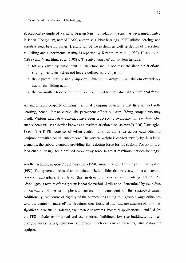
A practical example of a sliding bearing Seismic Isolation system has been implemented
in Japan. The system, named TASS, comprises rubber bearings, PTFE sliding bearings and
stainless steel bearing plates. Description of the system, as well as details of theoretical
modelling and experimental testing is reported by Kawamura et al. (1988), Hisano et al.
(1988) and Nagashima et al. (1988). The advantages of this system include:
• for any given dynamic input the structure should not resonate since the frictional
sliding mechanism does not have a defined natural period;
• the superstructure is stably supported since the bearings do not deform excessively
due to the sliding action;
• the transmitted horizontal input force is limited to the value of the frictional force.
An undesirable property of many frictional damping devices is that they are not self
centring, hence after an earthquake permanent off-set between sliding components may
result. Various innovative schemes have been proposed to overcome this problem. One
such scheme utilises a device known as a resilient-friction base isolator (R-FBI) (Mostaghel
1986). The R-FBI consists of teflon coated flat rings that slide across each other in
conjunction with a central rubber core. The vertical weight is carried entirely by the sliding
elements, the rubber elements providing the restoring force for the system. Frictional pre
load enables design for a defined break away force to resist maximum service loadings.
Another scheme, proposed by Zayas et al. (1990), makes use of a friction pendulum system
(FPS). The system consists of an articulated friction slider that moves within a concave or
convex semi-spherical surface; this motion produces a self centring action. An
advantageous feature of this system is that the period of vibration, determined by the radius
of curvature of the semi-spherical surface, is independent of the supported mass.
Additionally, the centre of rigidity of the connections acting as a group always coincides
with the centre of mass of the structure, thus torsional motions are minimised; this has
significant benefits in isolating asymmetric structures. Potential applications identified for
the FPS include: symmetrical and asymmetrical buildings, low rise buildings, highway
bridges, water tanks, museum sculptures, electrical circuit breakers, and computer
equipment.
18
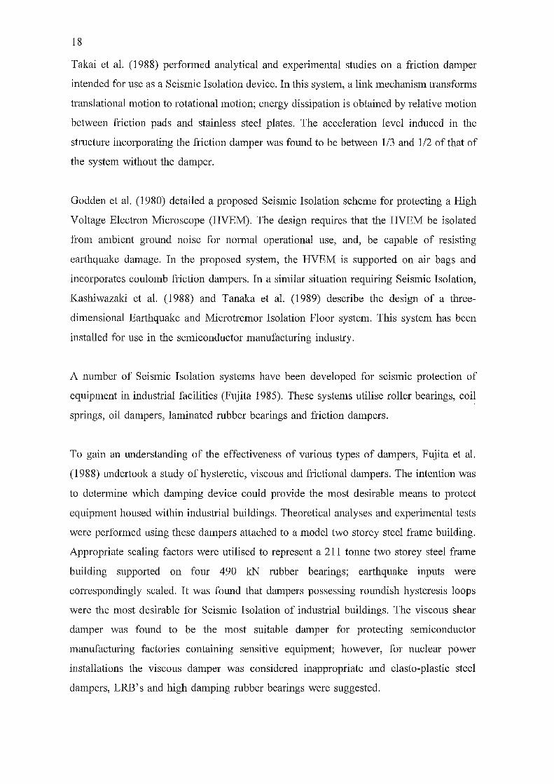
Takai et al. (1988) performed analytical and experimental studies on a friction damper
intended for use as a Seismic Isolation device. In this system, a link mechanism transforms
translational motion to rotational motion; energy dissipation is obtained by relative motion
between friction pads and stainless steel plates. The acceleration level induced in the
structure incorporating the friction damper was found to be between 1/3 and 1/2 of that of
the system without the damper.
Godden et al. (1980) detailed a proposed Seismic Isolation scheme for protecting a High
Voltage Electron Microscope (HVEM). The design requires that the HVEM be isolated
from ambient ground noise for normal operational use, and, be capable of resisting
earthquake damage. In the proposed system, the HVEM is suppmied on air bags and
incorporates coulomb friction dampers. In a similar situation requiring Seismic Isolation,
Kashiwazaki et al. (1988) and Tanaka et al. (1989) describe the design of a three
dimensional Earthquake and Microtremor Isolation Floor system. This system has been
installed for use in the semiconductor manufacturing industry.
A number of Seismic Isolation systems have been developed for seismic protection of
equipment in industrial facilities (Fujita 1985). These systems utilise roller bearings, coil
springs, oil dampers, laminated rubber bearings and friction dampers.
To gain an understanding of the effectiveness of various types of dampers, Fujita et al.
(1988) undertook a study of hysteretic, viscous and frictional dampers. The intention was
to determine which damping device could provide the most desirable means to protect
equipment housed within industrial buildings. Theoretical analyses and experimental tests
were performed using these dampers attached to a model two storey steel frame building.
Appropriate scaling factors were utilised to represent a 211 tonne two storey steel frame
building supported on four 490 kN rubber bearings; earthquake inputs were
correspondingly scaled. It was found that dampers possessing roundish hysteresis loops
were the most desirable for Seismic Isolation of industrial buildings. The viscous shear
damper was found to be the most suitable damper for protecting semiconductor
manufacturing factories containing sensitive equipment; however, for nuclear power
installations the viscous damper was considered inappropriate and elasto-plastic steel
dampers, LRB's and high damping rubber bearings were suggested.

19
(d) Advantages of seismic isolation
The principal aim of a Seismic Isolation scheme is to isolate a supported structure from
seismic disturbances, hence, reduce the level of excitation transmitted into the structure.
The advantages of Seismic Isolation can be summarised as follows.
(1) The benefits of seismically isolating structures include (Buckle 1985):
• simpler design procedures;
• use of non-ductile forms or components;
• construction economies;
• greater protection against earthquake induced damage (both structural and
non-structural);
• confinement of damage to a readily replaceable element.
(2) Seismic Isolation can provide economic benefits; numerous applications employing
Seismic Isolation have shown it to be cost effective in terms of both initial costs and
life cycle costs (Mayes et al. 1984, 1990). As an example, Seismic Isolation of the
Wellington Central Police Station cost 10% less than that of a ductile frame design
(McKay et al. 1990).
(3) For seismically isolated structures subjected to earthquakes possessmg response
spectra whose spectral accelerations reduce at longer periods (similar to that of El
Centro 1940 N-S), inertia forces and interstorey drifts of multi-storey structures can
be considerably reduced. For earthquakes greater than the design level, Seismic
Isolation buildings show fewer plastic hinges and much lower ductility demands when
compared with conventional ductile design structures (Andriano and Carr 1991).
(e) Seismic isolation applications in New Zealand
New Zealand has been recognised as a world leader in Seismic Isolation technology. Many
innovative Seismic Isolation devices and systems have been developed in New Zealand and
adopted both within the country and overseas. The following discussion details New
Zealand applications. Coverage of Seismic Isolation systems utilised worldwide is detailed
in a recently published book by Skinner et al. (1993).

20
At present seven buildings in New Zealand employ Seismic Isolation. A summary of these
structures and the isolation devices used are:
(1) William Clayton Building, Wellington: lead-rubber bearings
(Megget 1978)
(2) Union House, Auckland: sleeved piles and steel cantilever dissipators
(Boardman et al. 1983)
(3) Central Police Station, Wellington: sleeved piles and lead extrusion dampers
(Charleson et al. 1987)
(4) Wellington Newspapers Printing Press, Lower Butt: lead-rubber bearings
(Dowrick et al. 1991)
( 5) Parliament House, and,
(6) Parliament Library, Wellington: high damping bearings and lead-rubber bearings
(Poole and Clendon 1992; Robinson et al. 1995)
(7) Museum of New Zealand, Wellington: lead rubber bearings
(Robinson et al. 1995).
In New Zealand, 49 bridges employ Seismic Isolation systems (Skinner et al. 1993); the
majority of these applications use LRB's.
Two structures have been constructed that utilise rocking/stepping motion. A chimney,
located at the Christchurch airport, rests on lead pads and is designed to rock during strong
seismic excitation. In this system two cantilever type hysteretic dampers provide additional
energy dissipation (Sharpe and Skinner 1983).
Another structure, the South Rangitikei Rail Bridge, comprises twin concrete legs designed
to alternately lift off elastomeric bearings during seismic excitation. To provide damping
and control displacements, torsional beam hysteretic dampers are attached to each leg
(Cormack 1988).
In New Zealand, several items of high voltage electrical equipment have been protected
using Seismic Isolation. Capacitor banks at Haywards substation in Lower Butt are
seismically isolated using rubber bearings and hysteretic steel dampers (Cousins et al. 1991;
Skinner et al. 1993). In addition, circuit breakers as well as other items of electrical
21
equipment, have been fitted with Belleville washer dampers. These are discussed in
Chapter 7.
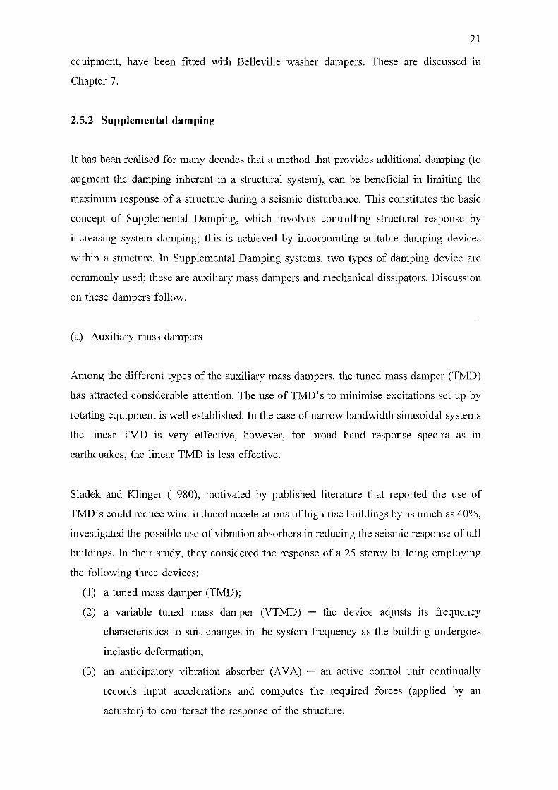
2.5.2 Supplemental damping
It has been realised for many decades that a method that provides additional damping (to
augment the damping inherent in a structural system), can be beneficial in limiting the
maximum response of a structure during a seismic disturbance. This constitutes the basic
concept of Supplemental Damping, which involves controlling structural response by
increasing system damping; this is achieved by incorporating suitable damping devices
within a structure. In Supplemental Damping systems, two types of damping device are
commonly used; these are auxiliary mass dampers and mechanical dissipators. Discussion
on these dampers follow.
(a) Auxiliary mass dampers
Among the different types of the auxiliary mass dampers, the tuned mass damper (TMD)
has attracted considerable attention. The use of TMD's to minimise excitations set up by
rotating equipment is well established. In the case of narrow bandwidth sinusoidal systems
the linear TMD is very effective, however, for broad band response spectra as in
earthquakes, the linear TMD is less effective.
Sladek and Klinger (1980), motivated by published literature that reported the use of
TMD's could reduce wind induced accelerations of high rise buildings by as much as 40%,
investigated the possible use of vibration absorbers in reducing the seismic response of tall
buildings. In their study, they considered the response of a 25 storey building employing
the following three devices:
(1) a tuned mass damper (TMD);
(2) a variable tuned mass damper (VTMD) - the device adjusts its frequency
characteristics to suit changes in the system frequency as the building undergoes
inelastic deformation;
(3) an anticipatory vibration absorber (AVA) - an active control unit continually
records input accelerations and computes the required forces (applied by an
actuator) to counteract the response of the structure.
22
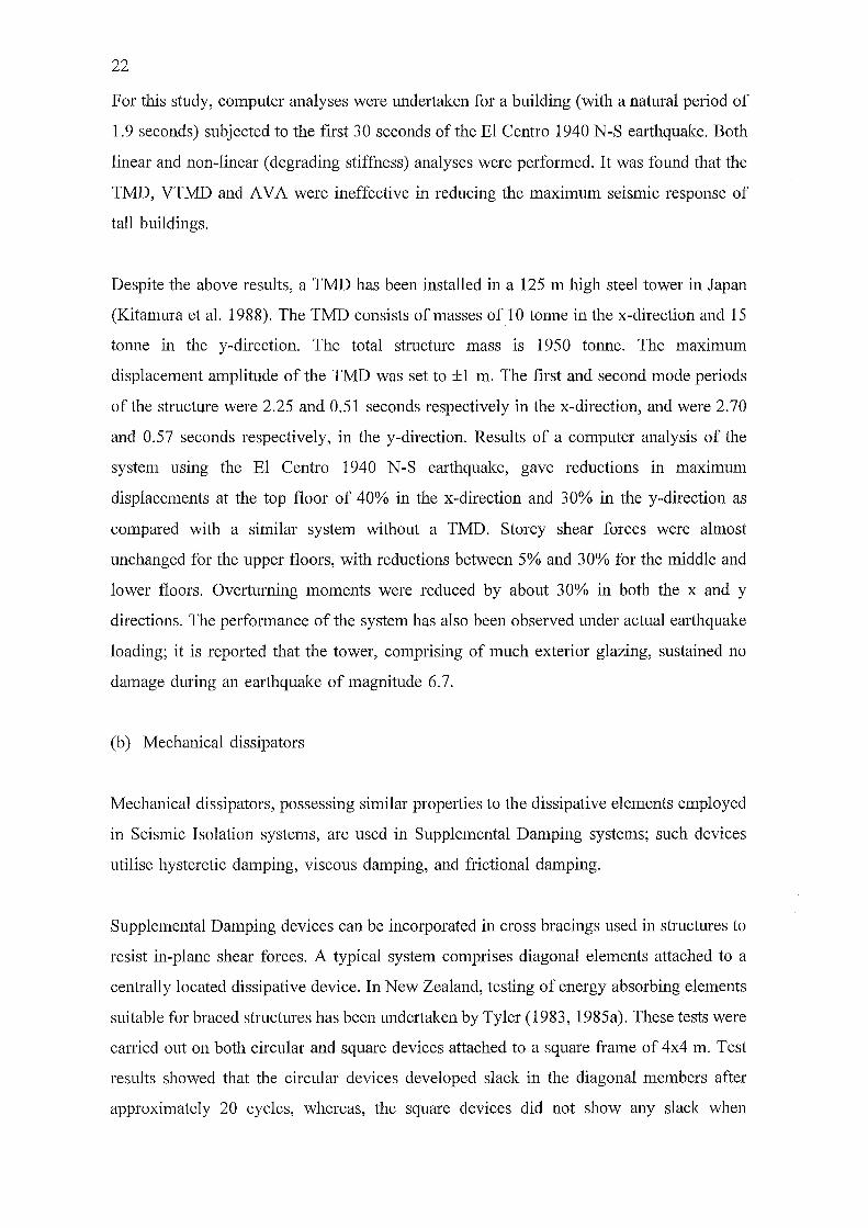
For this study, computer analyses were undertaken for a building (with a natural period of
1.9 seconds) subjected to the first 30 seconds of the El Centro 1940 N-S earthquake. Both
linear and non-linear (degrading stiffness) analyses were performed. It was found that the
TMD, VTMD and AVA were ineffective in reducing the maximum seismic response of
tall buildings.
Despite the above results, a TMD has been installed in a 125m high steel tower in Japan
(Kitamura et al. 1988). The TMD consists of masses of 10 tonne in the x-direction and 15
tonne in the y-direction. The total structure mass is 1950 tonne. The maximum
displacement amplitude of the TMD was set to ±1 m. The first and second mode periods
of the structure were 2.25 and 0.51 seconds respectively in the x-direction, and were 2. 70
and 0.57 seconds respectively, in the y-direction. Results of a computer analysis of the
system using the El Centro 1940 N-S earthquake, gave reductions in maximum
displacements at the top floor of 40% in the x-direction and 30% in the y-direction as
compared with a similar system without a TMD. Storey shear forces were almost
unchanged for the upper floors, with reductions between 5% and 30% for the middle and
lower floors. Ove1iurning moments were reduced by about 30% in both the x and y
directions. The performance of the system has also been observed under actual earthquake
loading; it is reported that the tower, comprising of much exterior glazing, sustained no
damage during an earthquake of magnitude 6.7.
(b) Mechanical dissipators
Mechanical dissipators, possessing similar properties to the dissipative elements employed
in Seismic Isolation systems, are used in Supplemental Damping systems; such devices
utilise hysteretic damping, viscous damping, and frictional damping.
Supplemental Damping devices can be incorporated in cross bracings used in structures to
resist in-plane shear forces. A typical system comprises diagonal elements attached to a
centrally located dissipative device. In New Zealand, testing of energy absorbing elements
suitable for braced structures has been undertaken by Tyler (1983, 1985a). These tests were
carried out on both circular and square devices attached to a square frame of 4x4 m. Test
results showed that the circular devices developed slack in the diagonal members after
approximately 20 cycles, whereas, the square devices did not show any slack when
23
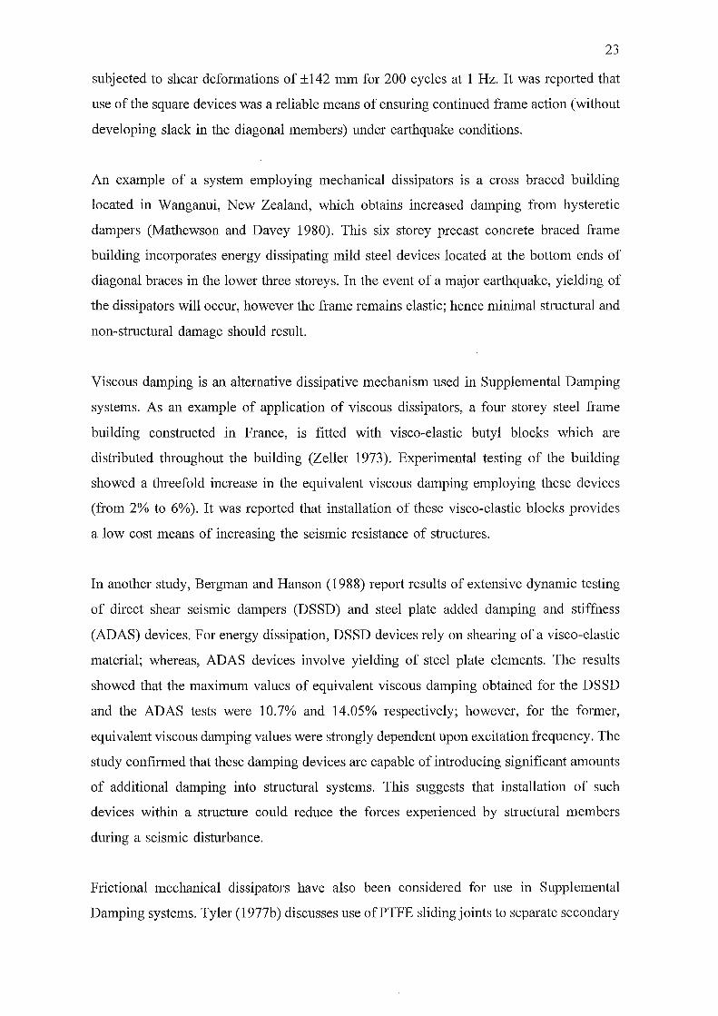
subjected to shear deformations of ±142 mm for 200 cycles at 1 Hz. It was repmied that
use of the square devices was a reliable means of ensuring continued frame action (without
developing slack in the diagonal members) under earthquake conditions.
An example of a system employing mechanical dissipators is a cross braced building
located in Wanganui, New Zealand, which obtains increased damping from hysteretic
dampers (Mathewson and Davey 1980). This six storey precast concrete braced frame
building incorporates energy dissipating mild steel devices located at the bottom ends of
diagonal braces in the lower three storeys. In the event of a major emihquake, yielding of
the dissipators will occur, however the frame remains elastic; hence minimal structural and
non-structural damage should result.
Viscous damping is an alternative dissipative mechanism used in Supplemental Damping
systems. As an example of application of viscous dissipators, a four storey steel frame
building constructed in France, is fitted with visco-elastic butyl blocks which are
distributed throughout the building (Zeller 1973). Experimental testing of the building
showed a threefold increase in the equivalent viscous damping employing these devices
(from 2% to 6%). It was reported that installation of these visco-elastic blocks provides
a low cost means of increasing the seismic resistance of structures.
In another study, Bergman and Hanson (1988) report results of extensive dynamic testing
of direct shear seismic dampers (DSSD) and steel plate added damping and stiffness
(ADAS) devices. For energy dissipation, DSSD devices rely on shearing of a visco-elastic
material; whereas, ADAS devices involve yielding of steel plate elements. The results
showed that the maximum values of equivalent viscous damping obtained for the DSSD
and the ADAS tests were 10.7% and 14.05% respectively; however, for the former,
equivalent viscous damping values were strongly dependent upon excitation frequency. The
study confirmed that these damping devices are capable of introducing significant amounts
of additional damping into structural systems. This suggests that installation of such
devices within a structure could reduce the forces experienced by structural members
during a seismic disturbance.
Frictional mechanical dissipators have also been considered for use in Supplemental
Damping systems. Tyler (1977b) discusses use ofPTFE sliding joints to separate secondary
24
components from the main structure of a building. These joints not only allow temperature
variation movement, but also provide additional damping during seismic and wind-induced
vibrations. Tyler (1985b) also completed tests on a frictional damper that dissipates seismic
energy during the relative displacement of structural elements. The damper comprised of
a sliding steel plate clamped against a brake lining. The test results for the friction damper
showed significant fluctuation in the shape of the force/deflection diagrams as a result of
slip-stick action. These results differ from those obtained by other researchers. Pall (1986),
for instance, showed results obtained from dynamic testing of a frictional damper, were
reliable and repeatable.
(c) Advantages of supplemental damping
Further research is required before stating any definite advantages in using auxiliary mass
dampers for protecting structural systems during earthquakes. However, the advantages of
using mechanical dissipators in Supplemental Damping systems have been reported as
follows.
(1) Supplemental Damping, by increasing the system damping, primarily reduces the
inertia loads induced in the structural system; this effect may provide (Thiel et al.
1986):
• increased protection of the structural system since member loads are reduced;
• a reduction in inelastic deformation sustained by the structure since some of the
input energy is dissipated by the mechanical dissipators;
• increased capability of the structure to resist subsequent earthquakes as inelastic
deformation of the structure's primary load carrying system is reduced;
• a reduction in non-structural damage since the maximum response of the
structure is reduced.
(2) The mechanical dissipators employed in Supplemental damping schemes, can be
simple, inexpensive, and exhibit reliable and repeatable characteristics. The devices
dissipate a portion of the seismic input energy, hence can reduce the energy that the
structure is required to absorb through inelastic deformation (Pall 1986).
25
2.5.3 Structural parameter adjustment
The Structural Parameter Adjustment method is a technique that utilises semi-active control
to adjust the parameters of a structural system; these parameters include mass, stiffness,
and damping. The system makes use of a control algorithm that optimises these parameters
so as to minimise the forces experienced by the structure members during a seismic
disturbance.
Experimental testing of this control concept has been reported by Kobori et al. (1988). For
this experiment, a model tluee storey steel frame building was built and tested on a shaker
table. The test results showed that the maximum response of the time history record
measured at the top floor of the building, was reduced to 114 of the response without
dynamic control. This system employed a central processing unit for carrying out the
optimisation of the structural parameters.
Though this control technique is still in its early stage of development, research in this
field is actively being pursued. However, before Structural Parameter Adjustment systems
become readily adopted, the system must demonstrate a fail-safe mechanism should the
control system power supply fail during a major earthquake; in addition, further work is
necessary to establish the economic feasibility of such schemes.
2.6 SUMMARY
The aseismic design methods used to protect engineering systems from seismic damage
have been detailed. These methods can be classified into two principal techniques: Strength
Design and Response Control. Strength Design involves using either the Working Stress
Method or the Strength Method. In the latter, structure detail provides plastic hinge
mechanisms that absorb inelastically the earthquake input energy.
In Response Control, specific control devices are incorporated within a structure to regulate
its response during an earthquake. Response Control utilises either active, passive, or semi
active control and can employ the following methods: Seismic Isolation, Supplemental
Damping, or Structural Parameter Adjustment. Details of these systems, the devices they
employ, developments and practical applications, have been presented.

26
Of the Response Control techniques, Seismic Isolation has attracted substantial attention
by researchers. This is because it is a simple, yet highly effective means of reducing
seismic loads experienced by structures during earthquakes. Extensive research, both
developmental and experimental, undertaken over the last 25 years has determined benefits
of Seismic Isolation schemes over conventional systems. Further, the performance of
several structures during actual earthquakes has demonstrated the effectiveness of this
technique. It is anticipated that recognition of Seismic Isolation as an effective method for
protecting structures during emihquakes will result in its increased use in seismic risk
regions throughout the world.
Chapter 3
RING SPRINGS: CHARACTERISTICS AND DESIGN
REQUIREMENTS
3.1 INTRODUCTION
27
Passive energy dissipation devices are used in earthquake-resistant applications; their
purpose is to absorb seismic input energy, thereby reduce structural deformations and hence
the level of loading experienced by a structure during an earthquake.
This chapter details the characteristics of a passive dissipation device known as a ring
spring. The ring spring stiffness equations and hysteresis diagram are detailed followed by
discussion on the design requirements for practical use of these devices. Subsequently,
solutions to the equations of motion for a bi-directional ring spring system are determined.
3.2 RING SPRINGS
3.2.1 Description and literature review
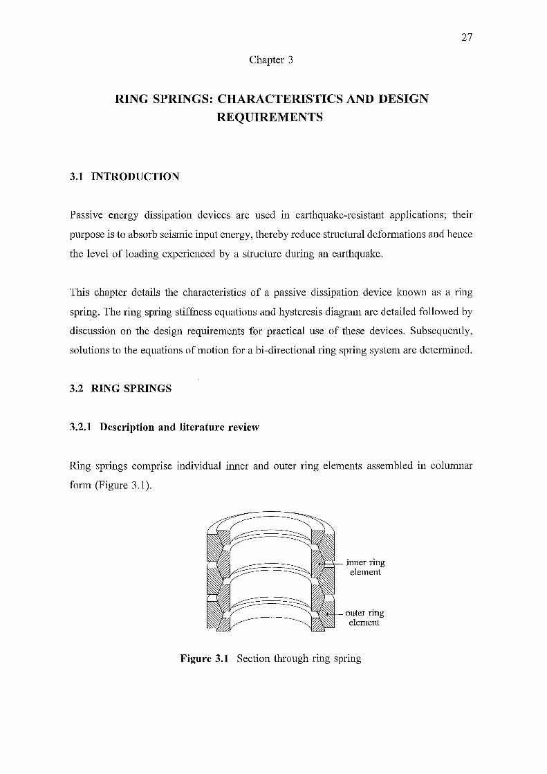
Ring springs comprise individual inner and outer ring elements assembled in columnar
form (Figure 3.1 ).
inner ring element
outer ring element
Figure 3.1 Section through ring spring
28
On application of axial load, wedge action at the interface causes the inner elements to
radially contract and the outer elements to radially expand (Figure 3 .2). Sliding action
between mating elements results in a large amount of energy being absorbed in overcoming
frictional forces. This absorbed energy may be as high as 60 to 70% of the total cycle
input energy (Simpson 1970).
applied load
expansion
expansion
applied load
Figure 3.2 Loaded ring spring
The ring spring was originally developed, and subsequently patented, in the 1920's by
Ringfeder GmbH, Germany, (Ringfeder 1925). A literature review on the subject of ring
springs showed surprisingly few publications. The first known paper on ring springs was
published in 1924 (Wikander 1924). Ring springs were considered suitable candidates for
use in drawbars in the railway industry due to their high energy absorption capability. In
a more comprehensive paper published two years later, Wikander outlined formulas for the
ring spring as well as presenting a hysteresis diagram obtained by testing a ring spring in
a universal testing machine (Wikander 1926). In 1933, Endsley reported on the use of ring
springs as draft gear springs for railway use. Details on ring springs can be found in
several text books, for example Berry (1961), Wahl (1963), and Gross (1966).
Ring springs are readily available commercially in load-carrying capacities ranging from
5 kN to 1800 kN, with larger load carrying capacities up to 10 000 kN also manufactured
(Ringfeder 1984).
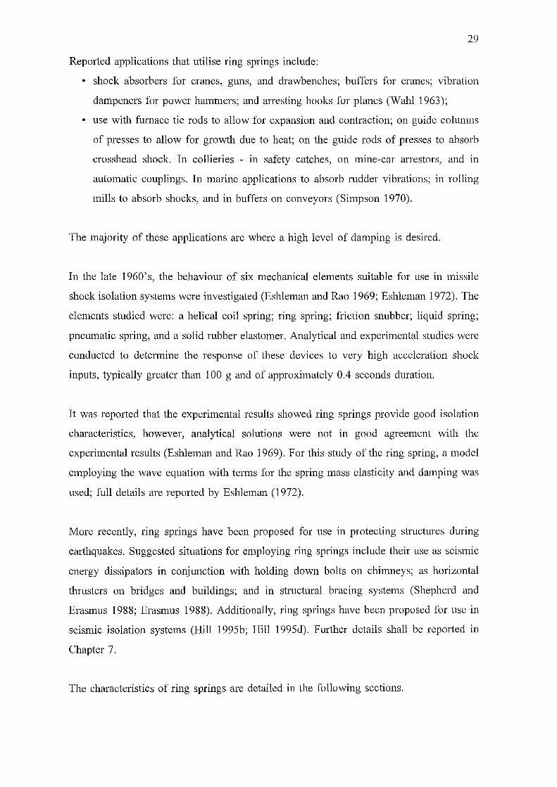
29
Reported applications that utilise ring springs include:
• shock absorbers for cranes, guns, and drawbenches; buffers for cranes; vibration
dampeners for power hammers; and arresting hooks for planes (Wahl 1963);
• use with furnace tie rods to allow for expansion and contraction; on guide columns
of presses to allow for growth due to heat; on the guide rods of presses to absorb
crosshead shock In collieries - in safety catches, on mine-car arrestors, and in
automatic couplings. In marine applications to absorb rudder vibrations; in rolling
mills to absorb shocks, and in buffers on conveyors (Simpson 1970).
The majority of these applications are where a high level of damping is desired.
In the late 1960's, the behaviour of six mechanical elements suitable for use in missile
shock isolation systems were investigated (Eshleman and Rao 1969; Eshleman 1972). The
elements studied were: a helical coil spring; ring spring; friction snubber; liquid spring;
pneumatic spring, and a solid rubber elastomer. Analytical and experimental studies were
conducted to determine the response of these devices to very high acceleration shock
inputs, typically greater than 100 g and of approximately 0.4 seconds duration.
It was reported that the experimental results showed ring springs provide good isolation
characteristics, however, analytical solutions were not in good agreement with the
experimental results (Eshleman and Rao 1969). For this study of the ring spring, a model
employing the wave equation with terms for the spring mass elasticity and damping was
used; full details are reported by Eshleman (1972).
More recently, ring springs have been proposed for use in protecting structures during
earthquakes. Suggested situations for employing ring springs include their use as seismic
energy dissipators in conjunction with holding down bolts on chimneys; as horizontal
thrusters on bridges and buildings; and in structural bracing systems (Shepherd and
Erasmus 1988; Erasmus 1988). Additionally, ring springs have been proposed for use in
seismic isolation systems (Hill 1995b; Hill 1995d). Further details shall be reported in
Chapter 7.
The characteristics of ring springs are detailed in the following sections.
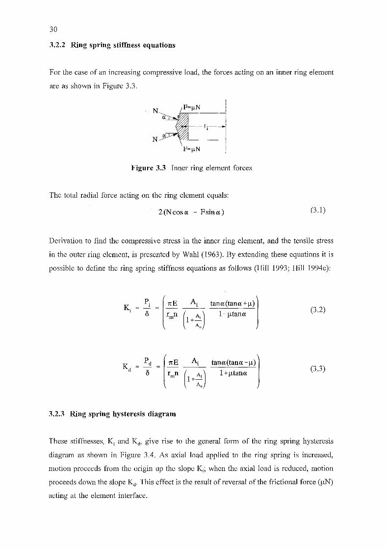
30
3.2.2 Ring spring stiffness equations
For the case of an increasing compressive load, the forces acting on an inner ring element
are as shown in Figure 3.3.
N I
~r------ r i ---j i !
Figure 3.3 Inner ring element forces
The total radial force acting on the ring element equals:
2 (N cos a - Fsina) (3.1)
Derivation to find the compressive stress in the inner ring element, and the tensile stress
in the outer ring element, is presented by Wahl (1963). By extending these equations it is
possible to define the ring spring stiffness equations as follows (Hill 1993; Hill 1994c):
(3.2)
(3.3)
3.2.3 Ring spring hysteresis diagram
These stiffnesses, Ki and Kd, give rise to the general form of the ring spring hysteresis
diagram as shown in Figure 3 .4. As axial load applied to the ring spring is increased,
motion proceeds from the origin up the slope Ki; when the axial load is reduced, motion
proceeds down the slope Kd. This effect is the result of reversal of the frictional force (~tN)
acting at the element interface.
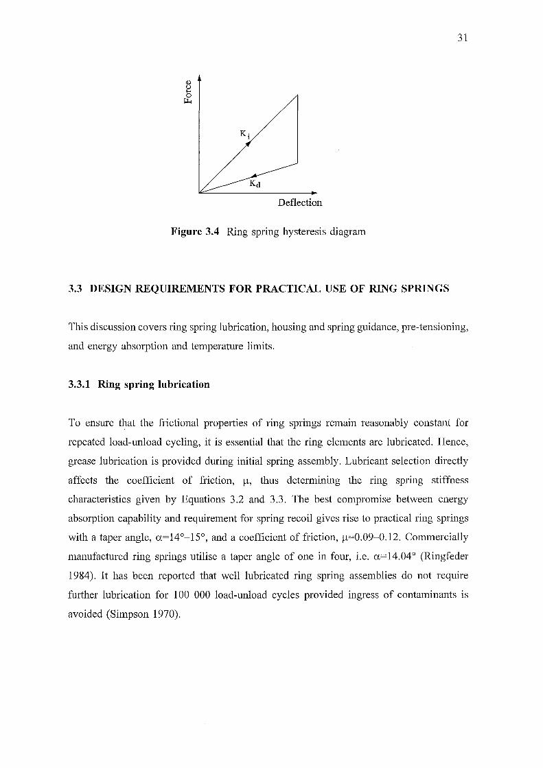
31
Deflection
Figure 3.4 Ring spring hysteresis diagram
3.3 DESIGN REQUIREMENTS FOR PRACTICAL USE OF RING SPRINGS
This discussion covers ring spring lubrication, housing and spring guidance, pre-tensioning,
and energy absorption and temperature limits.
3.3.1 Ring spring lubrication
To ensure that the frictional properties of ring springs remain reasonably constant for
repeated load-unload cycling, it is essential that the ring elements are lubricated. Hence,
grease lubrication is provided during initial spring assembly. Lubricant selection directly
affects the coefficient of friction, fl, thus determining the ring spring stiffness
characteristics given by Equations 3.2 and 3.3. The best compromise between energy
absorption capability and requirement for spring recoil gives rise to practical ring springs
with a taper angle, a=l4°-l5°, and a coefficient of friction, f-L=0.09-0.12. Commercially
manufactured ring springs utilise a taper angle of one in four, i.e. a=14.04° (Ringfeder
1984). It has been reported that well lubricated ring spring assemblies do not require
further lubrication for 100 000 load-unload cycles provided ingress of contaminants is
avoided (Simpson 1970).
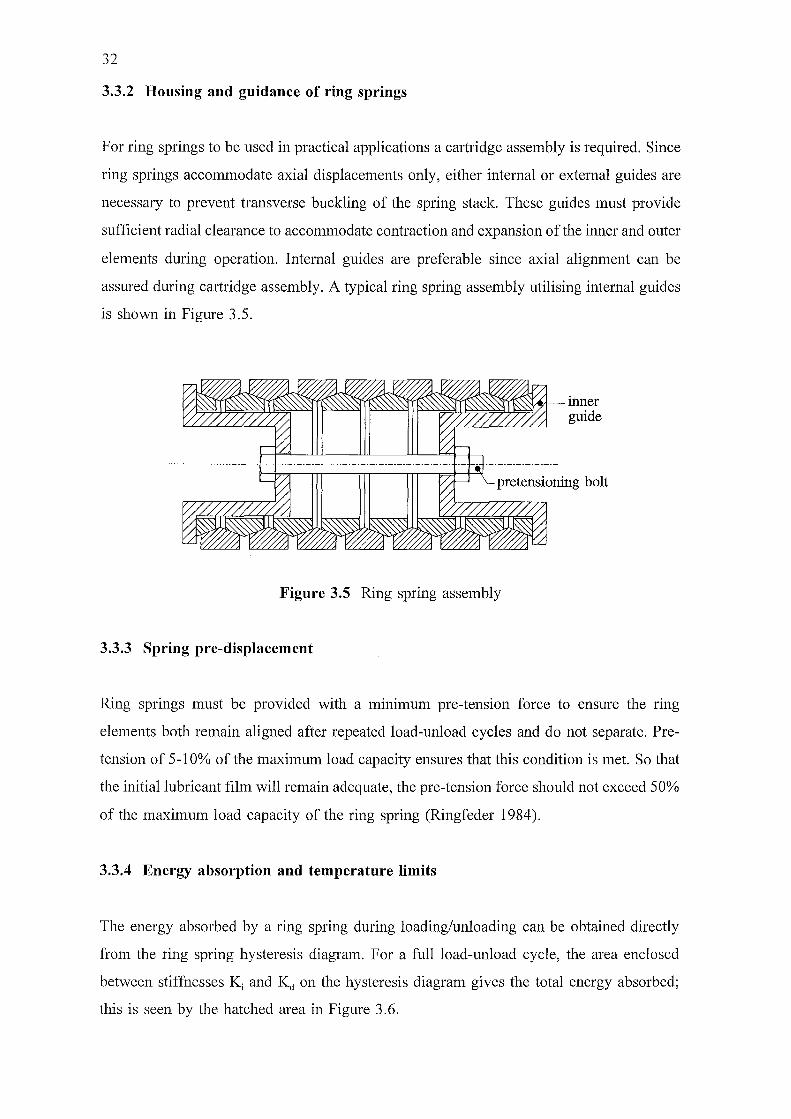
32
3.3.2 Housing and guidance of ring springs
For ring springs to be used in practical applications a cartridge assembly is required. Since
ring springs accommodate axial displacements only, either internal or external guides are
necessary to prevent transverse buckling of the spring stack. These guides must provide
sufficient radial clearance to accommodate contraction and expansion of the inner and outer
elements during operation. Internal guides are preferable since axial alignment can be
assured during cartridge assembly. A typical ring spring assembly utilising internal guides
is shown in Figure 3.5.
Figure 3.5 Ring spring assembly
3.3.3 Spring pre-displacement
inner guide
Ring springs must be provided with a minimum pre-tension force to ensure the ring
elements both remain aligned after repeated load-unload cycles and do not separate. Pre
tension of 5-l 0% of the maximum load capacity ensures that this condition is met. So that
the initial lubricant film will remain adequate, the pre-tension force should not exceed 50%
of the maximum load capacity of the ring spring (Ringfeder 1984).
3.3.4 Energy absorption and temperature limits
The energy absorbed by a ring spring during loading/unloading can be obtained directly
from the ring spring hysteresis diagram. For a full load-unload cycle, the area enclosed
between stiffnesses K; and Kd on the hysteresis diagram gives the total energy absorbed;
this is seen by the hatched area in Figure 3.6.
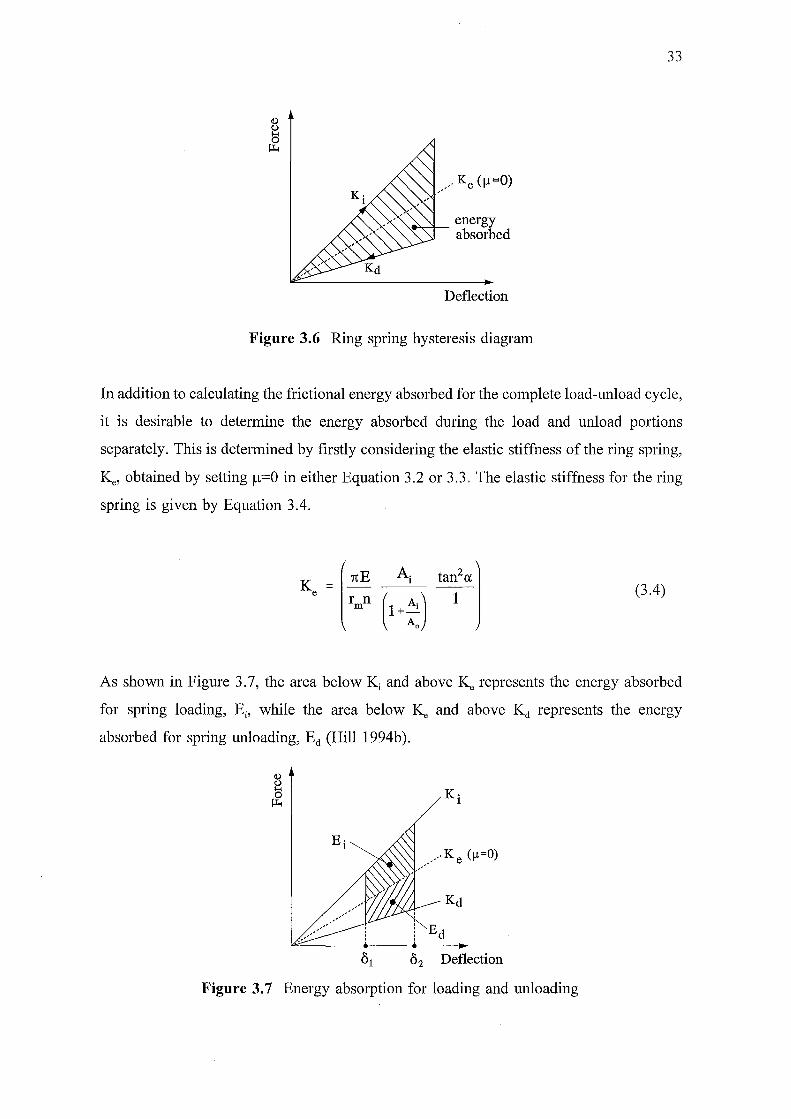
33
Deflection
Figure 3.6 Ring spring hysteresis diagram
In addition to calculating the frictional energy absorbed for the complete load-unload cycle,
it is desirable to determine the energy absorbed during the load and unload portions
separately. This is determined by firstly considering the elastic stiffness of the ring spring,
Ke, obtained by setting J.L=O in either Equation 3.2 or 3.3. The elastic stiffness for the ring
spring is given by Equation 3.4.
(3.4)
As shown in Figure 3. 7, the area below Ki and above Ke represents the energy absorbed
for spring loading, Ei, while the area below Ke and above Kd represents the energy
absorbed for spring unloading, Ed (Hill 1994b).
K· 1
01 o2 Deflection
Figure 3. 7 Energy absorption for loading and unloading
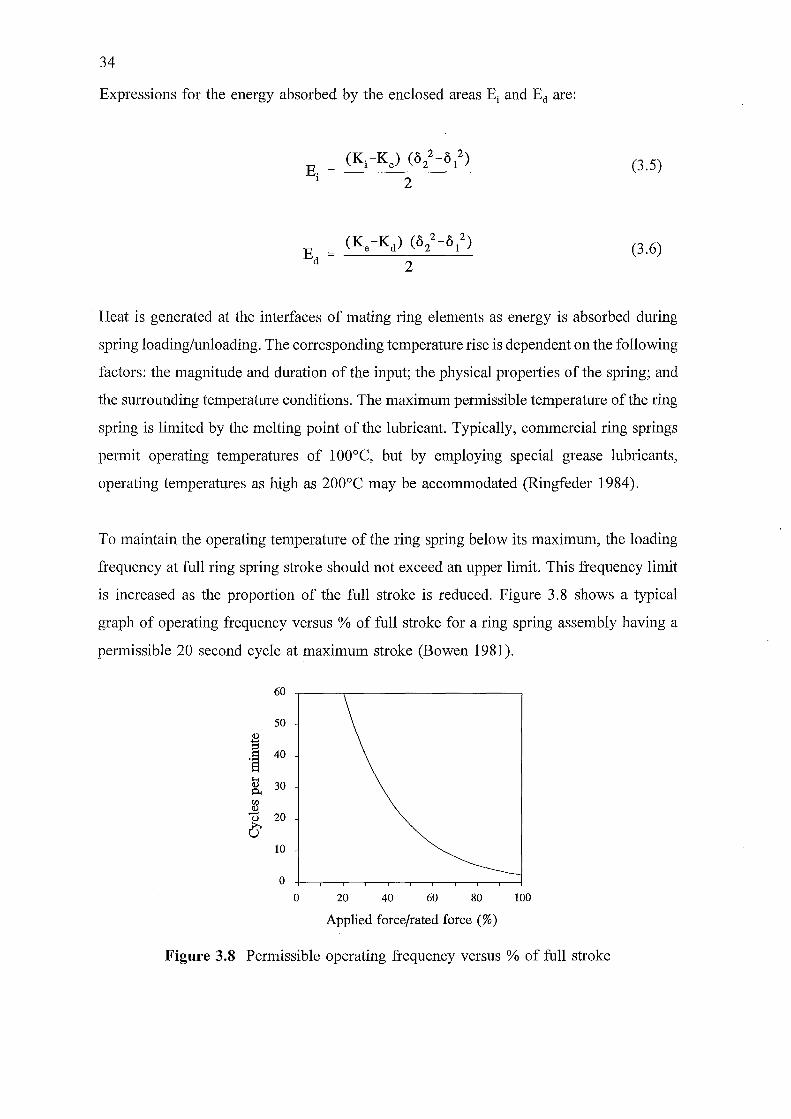
34
Expressions for the energy absorbed by the enclosed areas Ei and Ed are:
(Ki-Ke) (o/-o/) 2
(Ke -Kd) (o/-o /) 2
(3.5)
(3.6)
Heat is generated at the interfaces of mating ring elements as energy is absorbed during
spring loading/unloading. The corresponding temperature rise is dependent on the following
factors: the magnitude and duration of the input; the physical properties of the spring; and
the surrounding temperature conditions. The maximum permissible temperature of the ring
spring is limited by the melting point of the lubricant. Typically, commercial ring springs
permit operating temperatures of 1 00°C, but by employing special grease lubricants,
operating temperatures as high as 200°C may be accommodated (Ringfeder 1984).
To maintain the operating temperature of the ring spring below its maximum, the loading
frequency at full ring spring stroke should not exceed an upper limit. This frequency limit
is increased as the proportion of the full stroke is reduced. Figure 3. 8 shows a typical
graph of operating frequency versus % of full stroke for a ring spring assembly having a
permissible 20 second cycle at maximum stroke (Bowen 1981).
60
50 <I)
~ ·§ 40
~ 30 Pi {/)
~ 20
0 10
0
0 20 40 60 80 100
Applied force/rated force(%)
Figure 3.8 Permissible operating frequency versus % of full stroke
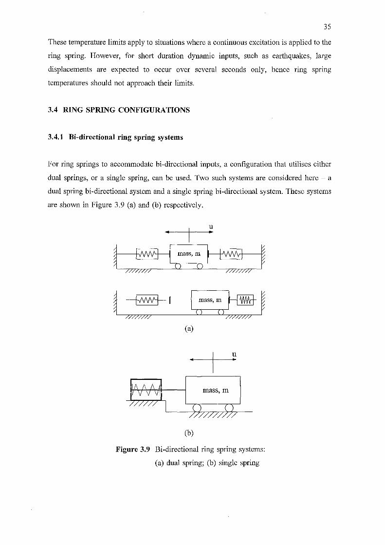
35
These temperature limits apply to situations where a continuous excitation is applied to the
ring spring. However, for short duration dynamic inputs, such as earthquakes, large
displacements are expected to occur over several seconds only, hence ring spring
temperatures should not approach their limits.
3.4 RING SPRING CONFIGURATIONS
3.4.1 Bi-directional ring spring systems
For ring springs to accommodate bi-directional inputs, a configuration that utilises either
dual springs, or a single spring, can be used. Two such systems are considered here - a
dual spring bi-directional system and a single spring bi-directional system. These systems
are shown in Figure 3.9 (a) and (b) respectively.
u ..
I m•&<, m l!!J () ()
(a)
u ..
mass, m
(b)
Figure 3.9 Bi-directional ring spring systems:
(a) dual spring; (b) single spring
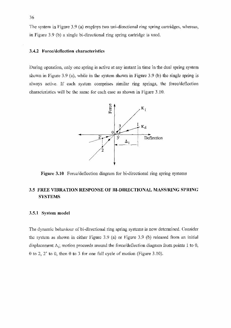
36
The system in Figure 3.9 (a) employs two uni-directional ring spring cartridges, whereas,
in Figure 3.9 (b) a single bi-directional ring spring cartridge is used.
3.4.2 Force/deflection characteristics
During operation, only one spring is active at any instant in time in the dual spring system
shown in Figure 3 .9 (a), while in the system shown in Figure 3 .9 (b) the single spring is
always active. If each system comprises similar ring springs, the force/deflection
characteristics will be the same for each case as shown in Figure 3.1 0.
2
K· 1
Deflection
Figure 3.10 Force/deflection diagram for bi-directional ring spring systems
3.5 FREE VIBRATION RESPONSE OF BI-DIRECTIONAL MASS/RING SPRING
SYSTEMS
3.5.1 System model
The dynamic behaviour of bi-directional ring spring systems is now determined. Consider
the system as shown in either Figure 3.9 (a) or Figure 3.9 (b) released from an initial
displacement .!11; motion proceeds around the force/deflection diagram from points 1 to 0,
0 to 2, 2' to 0, then 0 to 3 for one full cycle of motion (Figure 3.10).

37
3.5.2 Governing equation of motion
To determine the dynamic response of this system, the equation of motion can be
expressed as:
mii + k*u = 0 (3.7)
where:
- k* is the particular stiffness on the force/deflection diagram at the instant of motion
considered (either Ki or KJ;
- u(t) is the displacement of the mass.
The system has two separate natural frequencies, a natural frequency on the lower slope,
_ (Kd]+ w --nd m
(3.8)
a natural fi·equency on the upper slope,
_ (Ki]+ w.- -m m
(3.9)
and four cycle 1/4 periods, comprising both T1 and T2, where:
T = 7t (3.10) 1 2wnd
T2 7t (3.11) --
2wni
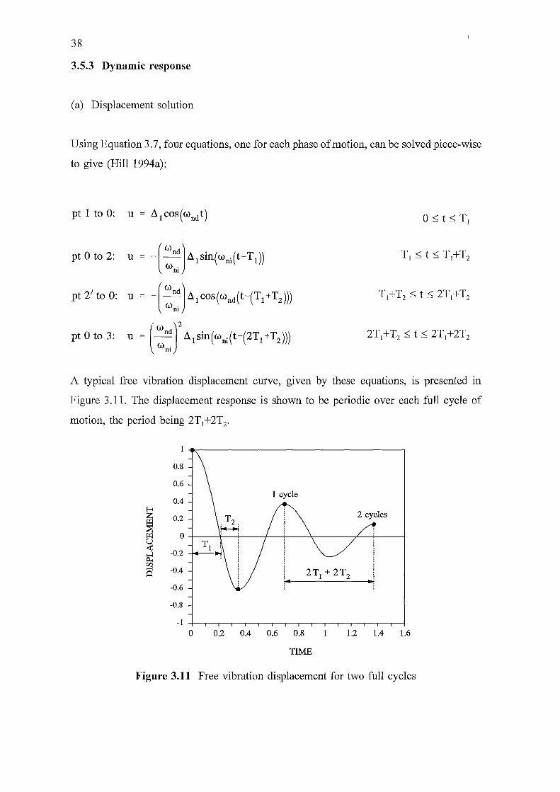
38
3.5.3 Dynamic response
(a) Displacement solution
Using Equation 3. 7, four equations, one for each phase of motion, can be solved piece-wise
to give (Hill 1994a):
pt 0 to 2: u o -( :::JLI 1sin("',1(t-Tl))
pt 21 to 0: u o -(:::)a, cos("',,(t-(T1+T2 )))
pt o to 3: u 0 ( ::)' a,sin("'m(t-(2T,+T,JJl
A typical free vibration displacement curve, given by these equations, is presented in
Figure 3 .11. The displacement response is shown to be periodic over each full cycle of
motion, the period being 2T1+2T2•
1
0.8
0.6
0.4 1 cycle
~ 0.2
j:il 0 u Tl j -0.2 Po< ga
-0.4 0
-0.6
-0.8
-1 0 0.2 0.4 0.6 0.8 1 1.2 1.4 1.6
TIME
Figure 3.11 Free vibration displacement for two full cycles

39
(b) Acceleration solution
The acceleration solution can also be solved in a piece-wise manner. This gives:
pt 1 to 0: ii = -(c.und)2~1cos(c.undt)
pt 0 to 2: ii = ( c.und. c.uni) ~ 1 sin( c.uni (t-T !))
pt 21 to 0: ii U)nd ( 'l = c.uni ~1 cos(c.unct(t-(Tl +T2)))
pt 0 to 3: ii -(c.unct)2 ~1 sin(c.uru(t-(2Tl +T2)))
A typical free vibration acceleration curve, given by these equations, is presented in Figure
3.12. The steep lines shown on the response between points 2 and 2', and 3 and 3',
correspond to a stiffness change, from Ki to Kd, as motion reverses direction (Figure 3 .1 0).
1
0.8
0.6
0.4
a 0.2
~ 0
5 -0.2 B u -0.4 < -0.6
-0.8
-1
0 0.2 0.4 0.6 0.8 1 1.2 1.4 1.6
TIME
Figure 3.12 Free vibration acceleration for two full cycles
40
3.5.4 Ring spring damping factor
From the displacement solution, the initial displacement 111 is shown to reduce over one
full cycle by a factor given by:
Utilising Equations 3.2 and 3.3 and Equations 3.8 and 3.9, this gives:
y (tana -f..l) (1-f..Ltana) (1 +f..Ltana) (tana +f..L)
(3.12)
(3.13)
After q cycles, the initial displacement reduces by a factor of yq. For a ring spring with a
taper angle of a=15° and coefficient of friction f.t=0.12, the displacement reduces after one,
two and three cycles to 0.358, 0.128 and 0.046 of the initial displacement respectively. The
free vibration decay curve shown in Figure 3.11 is for a=15° and f.t=0.12. These results
show that free vibration oscillations reduce to small values within a few cycles of motion.
The above equations can be used to define the ring spring damping factor. For free
vibration decay the damping factor can be approximated from the ratio of displacement
amplitudes measured after q cycles:
(3.14)
Utilising Equation 3.13 the ring spring damping factor is given by (Hill 1994b):
_1 ln(l)
2n y (3.15)
Thus, the damping factor for the ring spring is a function of both the spring taper angle,
a, and the coefficient of friction, fl·

41
For ring springs with a taper angle, a=l4°-15°, and a coefficient offriction, !-1=0.09-0.12,
the above equations give the damping factor as 0.119:::::; s:::::; 0.176; an equivalent viscous
damping value of between 11.9% and 17.6%.
3.6 SUMMARY
Ring springs are passive devices capable of absorbing as much as 60-70% of the total
cycle input energy. Their stiffness equations and hysteresis characteristics have been
detailed. The requirements for utilising ring springs in practical systems have been
presented. Consideration has been given to ring spring lubrication, guidance, pre
tensioning, and energy absorption and temperature limits.
Solutions to the equations of motion for a bi-directional ring spring system have been
determined. These show that free vibration oscillations diminish within a few cycles of
motion. Ring springs have damping factors of between 11.9% and 17.6%.

42
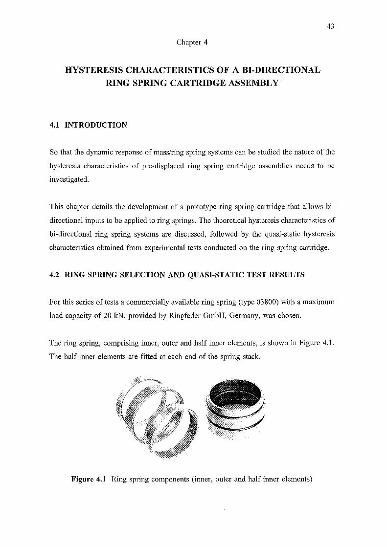
Chapter 4
HYSTERESIS CHARACTERISTICS OF A BI-DIRECTIONAL
RING SPRING CARTRIDGE ASSEMBLY
4.1 INTRODUCTION
43
So that the dynamic response of mass/ring spring systems can be studied the nature of the
hysteresis characteristics of pre-displaced ring spring cartridge assemblies needs to be
investigated.
This chapter details the development of a prototype ring spring cartridge that allows bi
directional inputs to be applied to ring springs. The theoretical hysteresis characteristics of
bi-directional ring spring systems are discussed, followed by the quasi-static hysteresis
characteristics obtained from experimental tests conducted on the ring spring cartridge.
4.2 RING SPRING SELECTION AND QUASI-STATIC TEST RESULTS
For this series of tests a commercially available ring spring (type 03800) with a maximum
load capacity of 20 k:N, provided by Ringfeder GmbH, Germany, was chosen.
The ring spring, comprising inner, outer and half inner elements, is shown in Figure 4.1.
The half inner elements are fitted at each end of the spring stack.
Figure 4.1 Ring spring components (inner, outer and half inner elements)

44
4.2.1 Physical properties of the selected ring spring
Details of the chosen ring spring are presented in Figure 4.2 and in the specifications
below.
ring spring external diameter = 3 8.1 mm
ring spring internal diameter = 31.7 mm
free length of ring spring= 266.0 mm
n = 56 interfaces
tana = 0.25 (a = 14.04°)
)l 0.10
E 200 GPa
AD 14.12 mm2
Ai 11.09 mm2
rm 17.35 mm
4.2.2 Quasi-static hysteresis diagram
ri = 16.6 mm
Figure 4.2 Ring spring dimensions
To experimentally determine the hysteresis characteristics of the ring spring, a universal
testing machine at the University of Canterbury was used. Tests were performed for a
spring loading rate of 15 mm/min, and an unloading rate of 5 mm/min. The resultant
quasi-static hysteresis diagram is presented in Figure 4.3 (Hill 1995a).
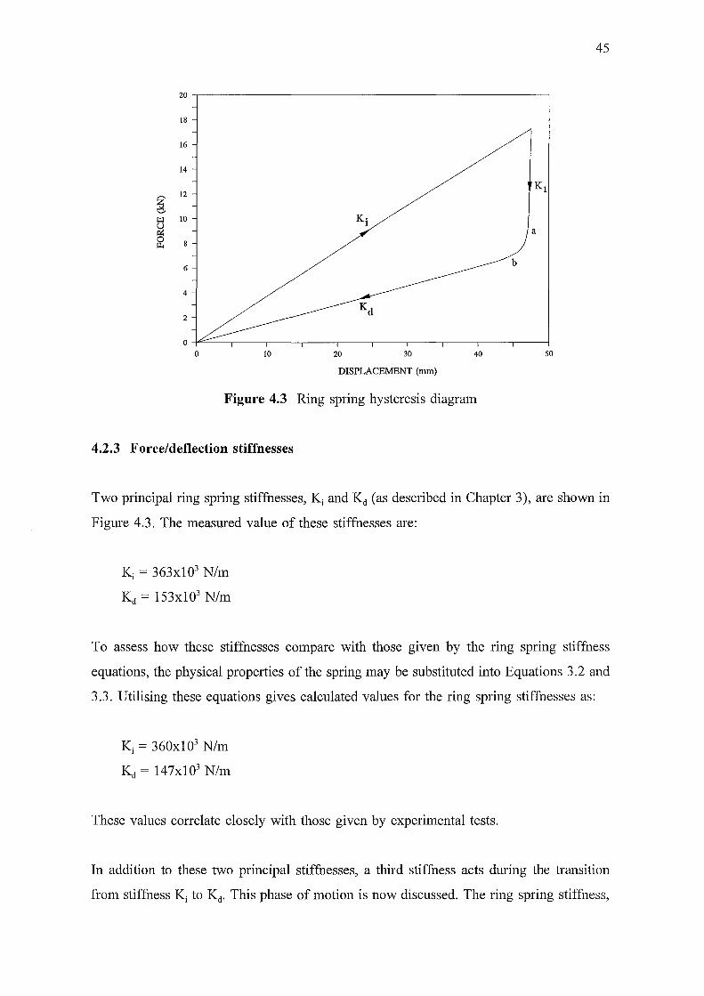
45
20
18
16
14
~ 12
~ 10
a 0 8 ~
6 b
4
2
0
0 10 20 30 40 50
DISPLACEMENT (mm)
Figure 4.3 Ring spring hysteresis diagram
4.2.3 Force/deflection stiffnesses
Two principal ring spring stiffnesses, Ki and Kd (as described in Chapter 3), are shown in
Figure 4.3. The measured value of these stiffnesses are:
Ki = 363xl 03 N/m
Kd = 153xl 03 N/m
To assess how these stiffnesses compare with those given by the ring spring stiffness
equations, the physical properties of the spring may be substituted into Equations 3 .2 and
3.3. Utilising these equations gives calculated values for the ring spring stiffnesses as:
Ki = 360xl 03 N/m
Kd = 147xl03 N/m
These values correlate closely with those given by experimental tests.
In addition to these two principal stiffnesses, a third stiffness acts during the transition
from stiffness Ki to Kd. This phase of motion is now discussed. The ring spring stiffness,
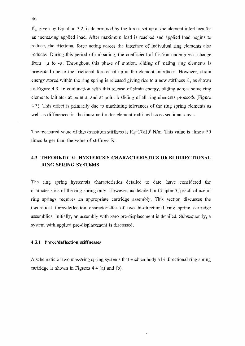
46
Ki, given by Equation 3 .2, is determined by the forces set up at the element interfaces for
an increasing applied load. After maximum load is reached and applied load begins to
reduce, the frictional force acting across the interface of individual ring elements also
reduces. During this period of unloading, the coefficient of friction undergoes a change
from +f.! to -f.!. Throughout this phase of motion, sliding of mating ring elements is
prevented due to the frictional forces set up at the element interfaces. However, strain
energy stored within the ring spring is released giving rise to a new stiffness K1 as shown
in Figure 4.3. In conjunction with this release of strain energy, sliding across some ring
elements initiates at point a, and at point b sliding of all ring elements proceeds (Figure
4.3). This effect is primarily due. to machining tolerances of the ring spring elements as
well as differences in the inner and outer element radii and cross sectional areas.
The measured value of this transition stiffness is K1= 17xl 06 N/m. This value is almost 50
times larger than the value of stiffness Ki.
4.3 THEORETICAL HYSTERESIS CHARACTERISTICS OF BI-DIRECTIONAL
RING SPRING SYSTEMS
The ring spring hysteresis characteristics detailed to date, have considered the
characteristics of the ring spring only. However, as detailed in Chapter 3, practical use of
ring springs requires an appropriate cartridge assembly. This section discusses the
theoretical force/deflection characteristics of two bi-directional ring spring cartridge
assemblies. Initially, an assembly with zero pre-displacement is detailed. Subsequently, a
system with applied pre-displacement is discussed.
4.3.1 Force/deflection stiffnesses
A schematic of two mass/ring spring systems that each embody a bi-directional ring spring
cartridge is shown in Figures 4.4 (a) and (b).
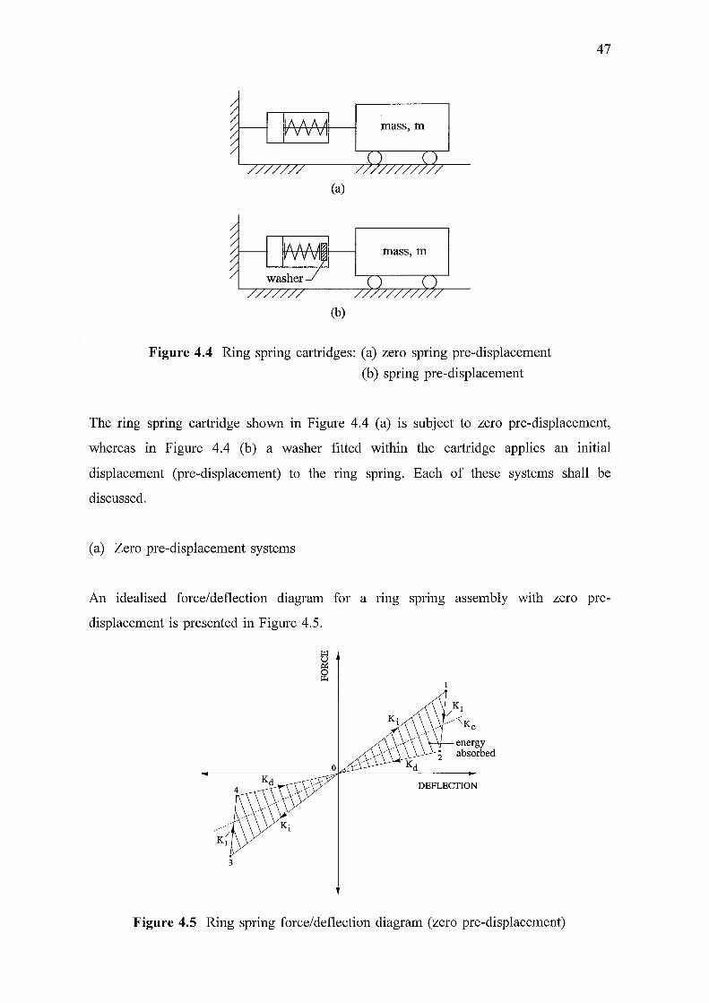
mass, m
(a)
mass, m
(b)
Figure 4.4 Ring spring cartridges: (a) zero spring pre-displacement
(b) spring pre-displacement
47
The ring spring cartridge shown in Figure 4.4 (a) is subject to zero pre-displacement,
whereas in Figure 4.4 (b) a washer fitted within the cartridge applies an initial
displacement (pre-displacement) to the ring spring. Each of these systems shall be
discussed.
(a) Zero pre-displacement systems
An idealised force/deflection diagram for a nng spring assembly with zero pre
displacement is presented in Figure 4.5.
energy 2 absorbed
DEFLECTION
3
Figure 4.5 Ring spring force/deflection diagram (zero pre-displacement)
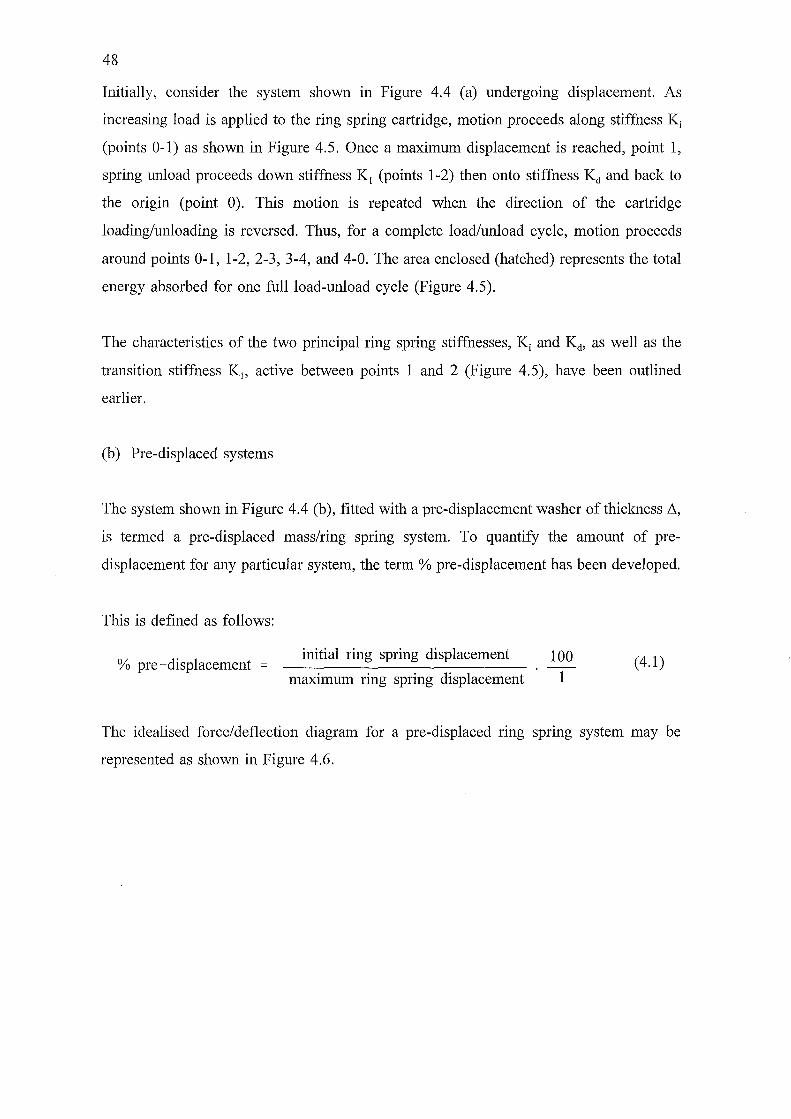
48
Initially, consider the system shown in Figure 4.4 (a) undergoing displacement. As
increasing load is applied to the ring spring cartridge, motion proceeds along stiffness Ki
(points 0-1) as shown in Figure 4.5. Once a maximum displacement is reached, point 1,
spring unload proceeds down stiffness K 1 (points 1-2) then onto stiffness Kd and back to
the origin (point 0). This motion is repeated when the direction of the cartridge
loading/unloading is reversed. Thus, for a complete load/unload cycle, motion proceeds
around points 0-1, 1-2, 2-3, 3-4, and 4-0. The area enclosed (hatched) represents the total
energy absorbed for one full load-unload cycle (Figure 4.5).
The characteristics of the two principal ring spring stiffnesses, Ki and Kd, as well as the
transition stiffness K 1, active between points 1 and 2 (Figure 4.5), have been outlined
earlier.
(b) Pre-displaced systems
The system shown in Figure 4.4 (b), fitted with a pre-displacement washer of thickness ~'
is termed a pre-displaced mass/ring spring system. To quantify the amount of pre
displacement for any particular system, the term % pre-displacement has been developed.
This is defined as follows:
% pre -displacement = initial ring spring displacement
maximum ring spring displacement
100 1
(4.1)
The idealised force/deflection diagram for a pre-displaced ring spring system may be
represented as shown in Figure 4.6.
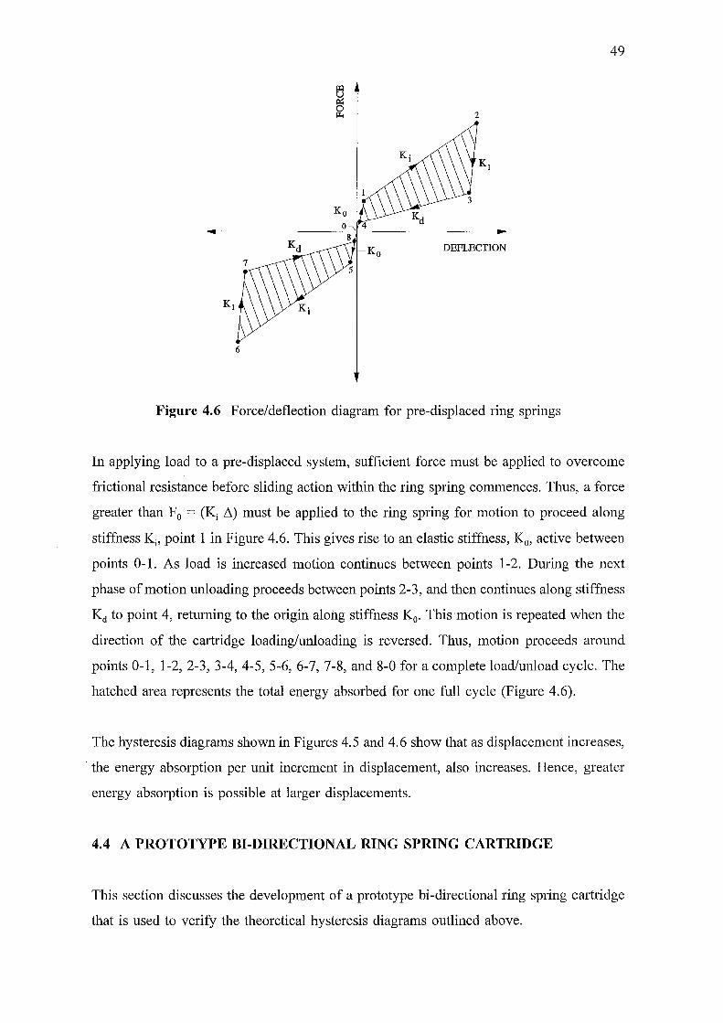
49
2
DEFLECTION
6
Figure 4.6 Force/deflection diagram for pre-displaced ring springs
In applying load to a pre-displaced system, sufficient force must be applied to overcome
frictional resistance before sliding action within the ring spring commences. Thus, a force
greater than F0 = (Ki ~) must be applied to the ring spring for motion to proceed along
stiffness Ki, point 1 in Figure 4.6. This gives rise to an elastic stiffness, K 0, active between
points 0-1. As load is increased motion continues between points 1-2. During the next
phase of motion unloading proceeds between points 2-3, and then continues along stiffness
Kd to point 4, returning to the origin along stiffness K0 • This motion is repeated when the
direction of the cartridge loading/unloading is reversed. Thus, motion proceeds around
points 0-1, 1-2, 2-3, 3-4, 4-5, 5-6, 6-7, 7-8, and 8-0 for a complete load/unload cycle. The
hatched area represents the total energy absorbed for one full cycle (Figure 4.6).
The hysteresis diagrams shown in Figures 4. 5 and 4. 6 show that as displacement increases,
· the energy absorption per unit increment in displacement, also increases. Hence, greater
energy absorption is possible at larger displacements.
4.4 A PROTOTYPE BI-DIRECTIONAL RING SPRING CARTRIDGE
This section discusses the development of a prototype bi-directional ring spring cartridge
that is used to verify the theoretical hysteresis diagrams outlined above.
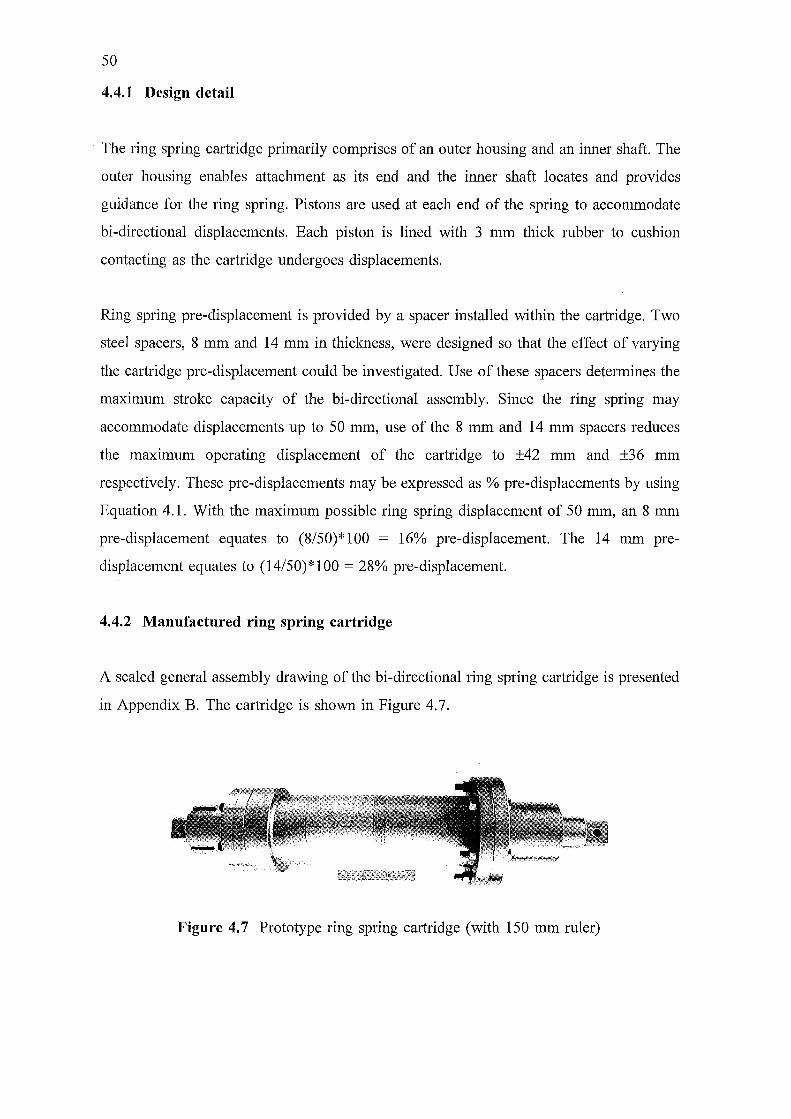
50
4.4.1 Design detail
The ring spring cartridge primarily comprises of an outer housing and an inner shaft. The
outer housing enables attachment as its end and the inner shaft locates and provides
guidance for the ring spring. Pistons are used at each end of the spring to accommodate
bi-directional displacements. Each piston is lined with 3 mm thick rubber to cushion
contacting as the cartridge undergoes displacements.
Ring spring pre-displacement is provided by a spacer installed within the cartridge. Two
steel spacers, 8 mm and 14 mm in thickness, were designed so that the effect of varying
the cartridge pre-displacement could be investigated. Use of these spacers determines the
maximum stroke capacity of the bi-directional assembly. Since the ring spring may
accommodate displacements up to 50 mm, use of the 8 mm and 14 mm spacers reduces
the maximum operating displacement of the cartridge to ±42 mm and ±36 mm
respectively. These pre-displacements may be expressed as% pre-displacements by using
Equation 4.1. With the maximum possible ring spring displacement of 50 mm, an 8 mm
pre-displacement equates to (8/50)*100 = 16% pre-displacement. The 14 mm pre
displacement equates to (14/50)*100 = 28% pre-displacement.
4.4.2 Manufactured ring spring cartridge
A scaled general assembly drawing of the bi-directional ring spring cartridge is presented
in Appendix B. The cartridge is shown in Figure 4.7.
Figure 4.7 Prototype ring spring cartridge (with 150 mm ruler)
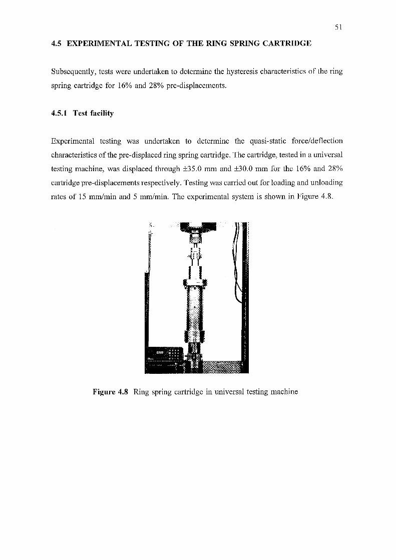
51
4.5 EXPERIMENTAL TESTING OF THE RING SPRING CARTRIDGE
Subsequently, tests were undertaken to determine the hysteresis characteristics of the ring
spring cartridge for 16% and 28% pre-displacements.
4.5.1 Test facility
Experimental testing was undertaken to determine the quasi-static force/deflection
characteristics of the pre-displaced ring spring cartridge. The cartridge, tested in a universal
testing machine, was displaced through ±35.0 mm and ±30.0 mm for the 16% and 28%
cartridge pre-displacements respectively. Testing was carried out for loading and unloading
rates of 15 mm/min and 5 mm/min. The experimental system is shown in Figure 4.8.
Figure 4.8 Ring spring cartridge in universal testing machine
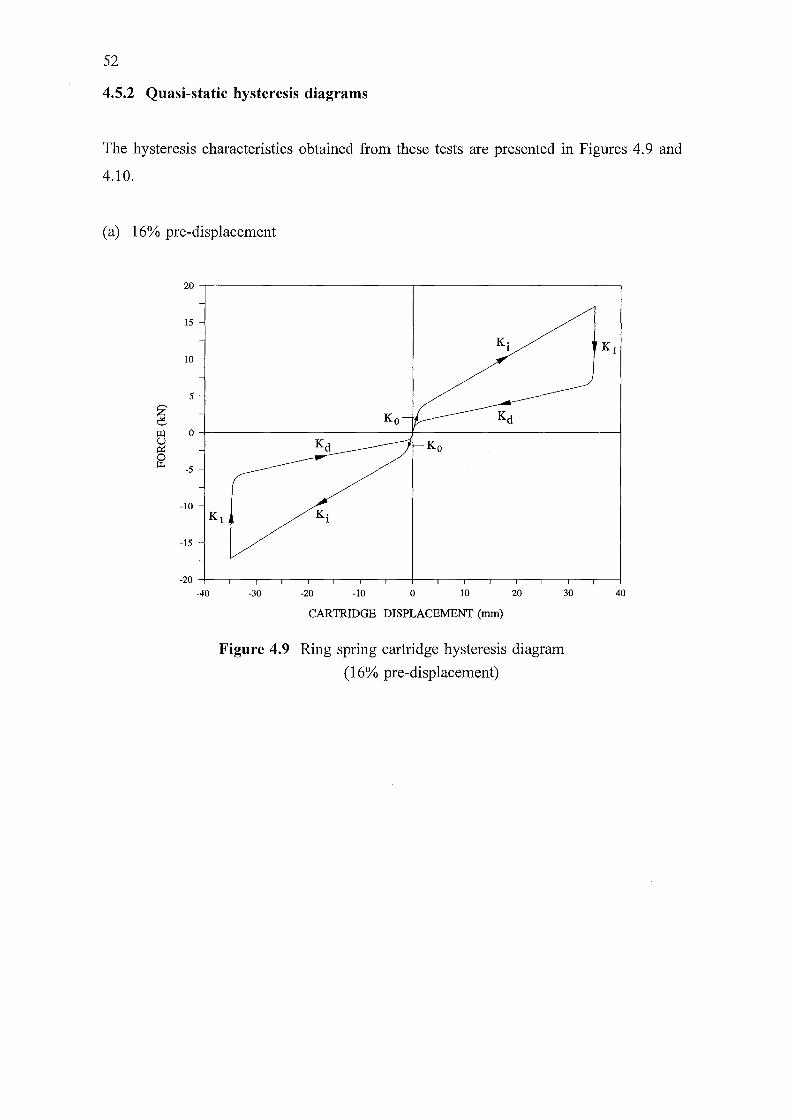
52
4.5.2 Quasi-static hysteresis diagrams
The hysteresis characteristics obtained from these tests are presented in Figures 4.9 and
4.10.
(a) 16% pre-displacement
20
15
10
5
~ ~
0
0 p:.
-5
-10
-15
-20
K1
-40 -30 -20 -10 0 10 20 30
CARTRIDGE DISPLACEMENT (nun)
Figure 4.9 Ring spring cartridge hysteresis diagram
(16% pre-displacement)
40
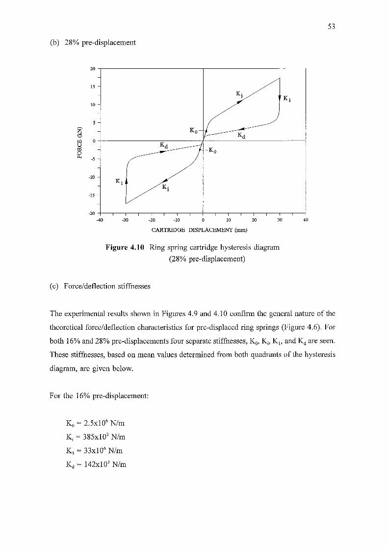
(b) 28% pre-displacement
20
15
10
5
~ ~
0
0 p..
-5
-10
-15
-20
-40 -30 -20
K· 1
-10 0 10
CARTRIDGE DISPLACEMENT (nun)
20 30
Figure 4.10 Ring spring cartridge hysteresis diagram
(28% pre-displacement)
(c) Force/ deflection stiffnesses
53
40
The experimental results shown in Figures 4.9 and 4.10 confirm the general nature of the
theoretical force/deflection characteristics for pre-displaced ring springs (Figure 4.6). For
both 16% and 28% pre-displacements four separate stiffnesses, K 0, Ki, K1, and Kd are seen.
These stiffnesses, based on mean values determined from both quadrants of the hysteresis
diagram, are given below.
For the 16% pre-displacement:
K0 = 2.5x10⁶ N/m
Ki = 385x103 N/m
K1 = 33x106 N/m
Kd = 142x103 N/m
54
For the 28% pre-displacement:
I<o = 2x10⁶ N/m
Ki = 410x103 N/m
K 1 = 38x106 N/m
Kd = 135x103 N/m
In addition, the force at the transition from stiffness Ka to Ki was measured as:
Fa= 2900 N (for the 16% pre-displacement)
Fa= 5500 N (for the 28% pre-displacement)
These forces compare with calculated values of Fa = 3080 Nand 5740 N (using Fa= Ki
6) for the 16% and 28% pre-displacements respectively.
Determination of the above hysteresis characteristics enables dynamic modelling of pre
displaced mass/ring spring systems to be undertaken. For this, the ring spring model is able
to be based upon four non-linear force/deflection stiffnesses - Ka, Ki, K 1, and Kd.
4.6 SUMMARY
The development and testing of a prototype ring spring cartridge suitable for applying bi
directional inputs to ring springs has been presented. Quasi-static testing of the cartridge
for two different pre-displacements has established that the hysteresis characteristics of pre
displaced ring spring systems comprise of four stiffness, Ka, Ki, K 1, and Kd. The dynamic
behaviour of ring spring systems may now be determined based upon these hysteresis
characteristics.
Chapter 5
FREE VIBRATION BEHAVIOUR OF PRE-DISPLACED AND
PRE-LOADED MASS/RING SPRING SYSTEMS
5.1 INTRODUCTION
55
Understanding of the dynamic behaviour of ring spring systems is a prerequisite to use of
these devices in applications subject to dynamic excitation. This chapter investigates the
dynamic behaviour of pre-displaced, pre-loaded, and pre-displaced pre-loaded single
degree-of-freedom (SDOF) mass/ring spring systems. Each of these systems is defined,
then their free vibration behaviour is detailed.
5.2 COMPUTER MODELLING OF SDOF MASS/RING SPRING SYSTEMS
In Chapter 3 the free vibration response of a SDOF mass/ring spring system was
determined by solving piece-wise the equations of motion. It was assumed that the ring
spring hysteresis characteristics comprised of only two stiffnesses, Ki and Kct, thus, making
it relatively easy to determine the free vibration response.
However, for practical ring spnng systems, the hysteresis diagram consists of four
stiffnesses: K0, Ki, K1 and Kct. To determine the free vibration response of systems with
these stiffnesses, it is difficult and cumbersome to solve the equations of motion for the
system in a piece-wise manner. A more convenient method for determining the dynamic
response is to employ a numerical integration technique. This allows the dynamic response
of a non-linear system to be determined.
5.2.1 Numerical integration method
A numerical technique, the Newmark (B = 0.25) constant average acceleration method
(Newmark 1962) was chosen to determine the dynamic response of the SDOF mass/ring
spring systems to be analysed. This method was selected as it is unconditionally stable.
56
The equations formulated using the Newmark method are detailed in several text books,
eg. Craig (1981), and are not restated here.
5.2.2 Ring spring model computer algorithm
To enable mass/ring sprmg systems to be analysed, a ring spring model has been
developed. The model is based upon the non-linear force/deflection characteristics of the
ring spring and uses five variables that fully define the ring spring hysteresis
characteristics. These are the four stiffnesses: Ko, Ki, K 1, and Kd and the ring spring pre
displacement.
In addition, a computer algorithm was written that embodies the ring spring model and
tracks the current stiffness on the hysteresis diagram at any given instant in time. The ring
spring model computer algorithm is presented in Appendix A. Further discussion of this
algorithm is reported in Chapter 7.
5.2.3 Types of ring spring systems considered in the study
The following sections detail the free vibration behaviour of:
• pre-displaced ring spring systems,
• pre-loaded ring spring systems,
• pre-displaced pre-loaded ring spring systems.
5.3 FREE VIBRATION BEHAVIOUR OF PRE-DISPLACED RING SPRING
SYSTEMS
This section details the dynamic response of a SDOF mass/ring spring system for both zero
and 16% pre-displacement.
5.3.1 System model
The model for a SDOF pre-displaced mass/ring spring system consists of a spring cartridge
attached to a mass as shown in Figure 5 .1. In (a) the system has zero pre-displacement,
whereas in (b) the cartridge, fitted with a washer, is pre-displaced. These systems have
been detailed in Chapter 4.
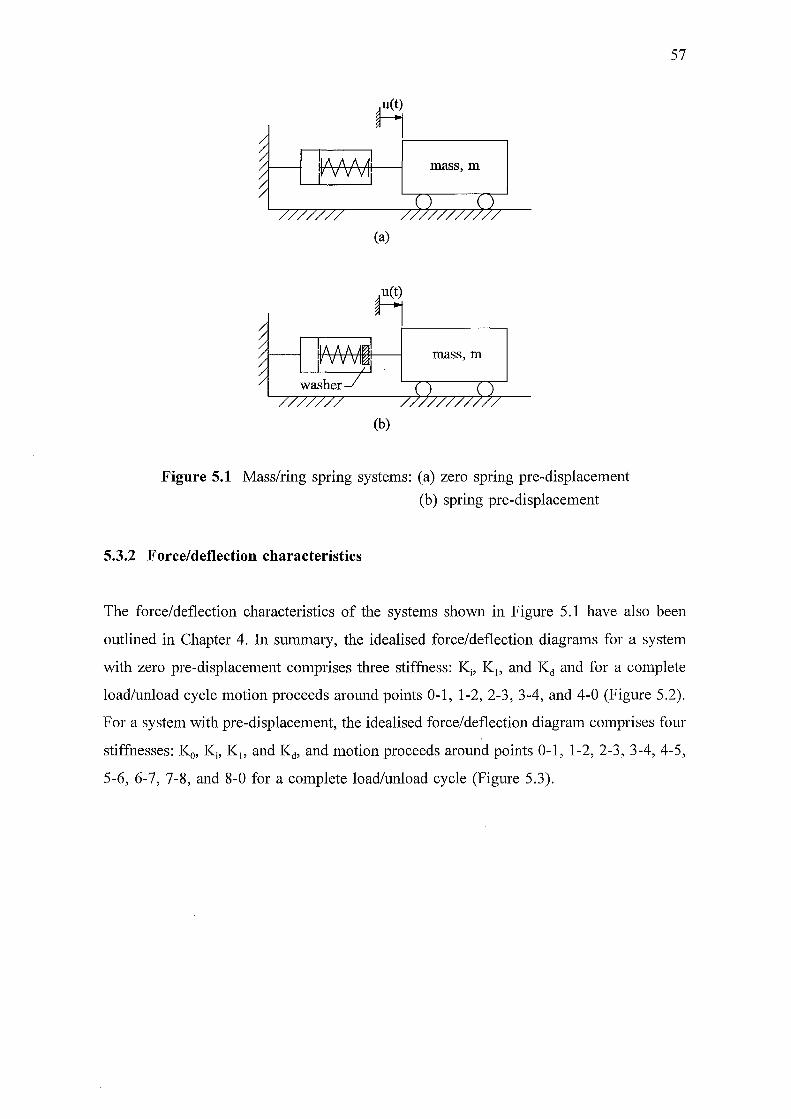
~ ;---------, mass, m
(a)
mass, m
(b)
Figure 5.1 Mass/ring spring systems: (a) zero spring pre-displacement
(b) spring pre-displacement
5.3.2 Force/deflection characteristics
57
The force/deflection characteristics of the systems shown in Figure 5.1 have also been
outlined in Chapter 4. In summary, the idealised force/deflection diagrams for a system
with zero pre-displacement comprises three stiffness: Ki, K1, and Kct and for a complete
load/unload cycle motion proceeds around points 0-1, 1-2, 2-3, 3-4, and 4-0 (Figure 5.2).
For a system with pre-displacement, the idealised force/deflection diagram comprises four
stiffnesses: K0, Ki, K1, and Kct, and motion proceeds around points 0-1, 1-2, 2-3, 3-4, 4-5,
5-6, 6-7, 7-8, and 8-0 for a complete load/unload cycle (Figure 5.3).
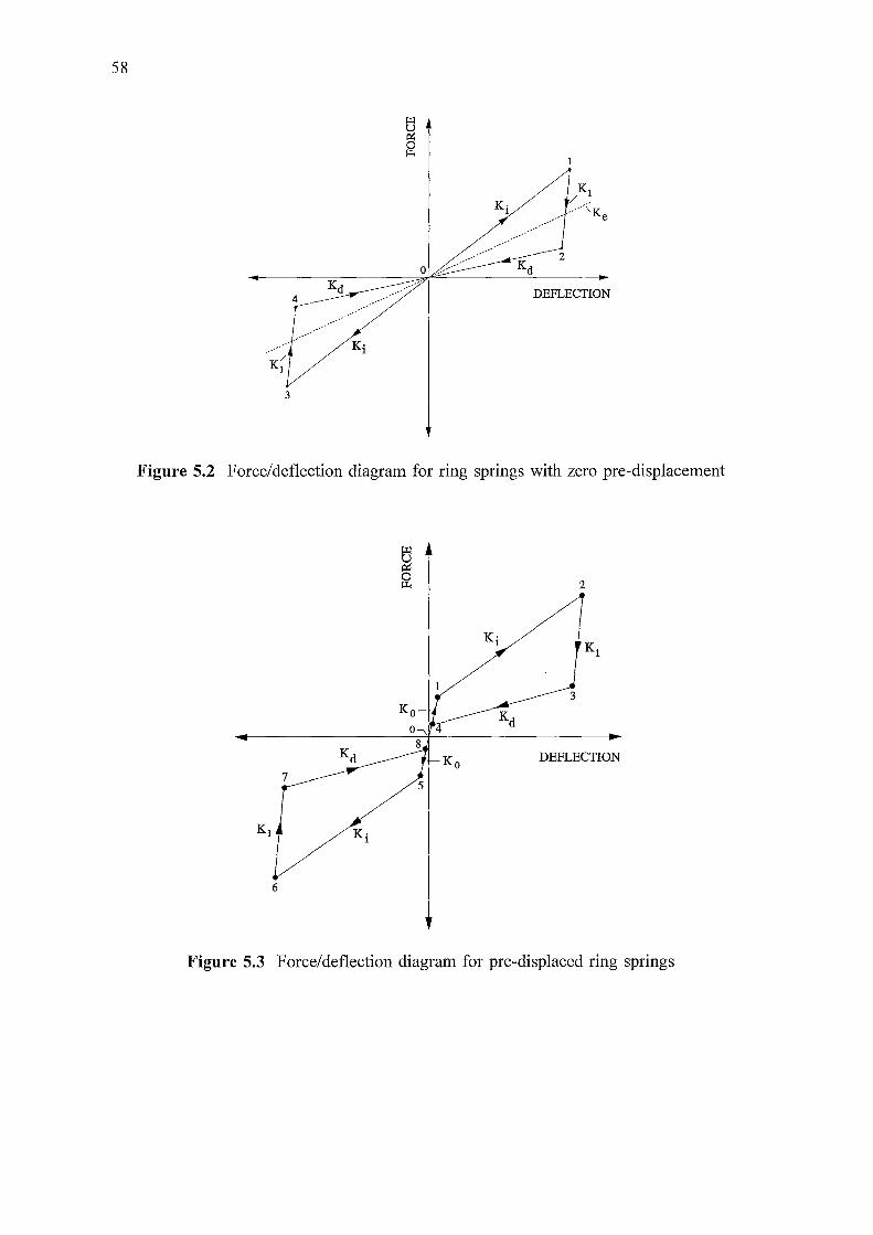
58
DEFLECTION
3
Figure 5.2 Force/deflection diagram for ring springs with zero pre-displacement
7
6
K· 1
2
3
DEFLECTION
Figure 5.3 Force/deflection diagram for pre-displaced ring springs
59
5.3.3 Equation of motion
The generalised equation of motion for a pre-displaced mass/ring spring system is:
mii + k*u = 0 (5.1)
where:
- k* is the particular stiffness on the force/deflection diagram at the instant of motion
considered (either Ko, Ki, K 1, or Kd); and
- u(t) is the displacement of the mass.
The following parameters have been used in analysing the dynamic response of the
mass/ring spring systems reported in this chapter:
Ko = 2.5x10⁶ N/m
~ = 385x103 N/m
K 1 = 33x106 N/m
Kd = 142x103 N/m
m = 472 kg
These stiffnesses were obtained from tests carried out on the prototype ring spring cartridge
reported in Chapter 4. The selected mass was chosen to correspond with that of an item
of equipment available for use in subsequent experimental testing.
5.3.4 Dynamic response
Utilising these values in the computer algorithm, the free vibration response of a mass/ring
spring system with zero, and with 16% pre-displacement, was determined. The systems,
as shown in Figure 5.1 (a) and (b), were each released from an initial displacement of 40
mm. Their displacement and acceleration responses are presented in Figures 5.4 and 5.5.
Further, force/deflection response curves for these systems are given in Figures 5.6 (a) and
(b). These diagrams give plots of the ring spring hysteresis characteristics developed during
the response.
Discussion of the results obtained for the pre-displaced systems follow.
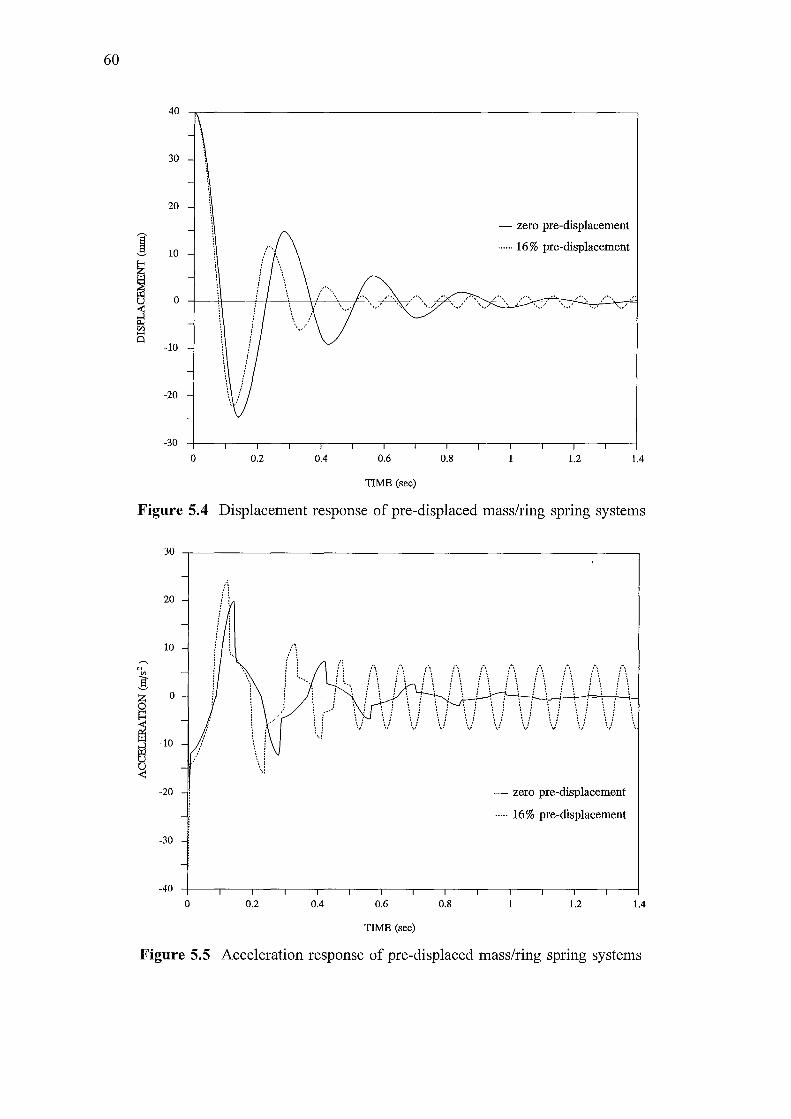
60
40
30
20
I 10
!i ~ ~
0
en ...... Q
-10
-20
-30
0 0.2 0.4 0.6
TIME (sec)
0.8
- zero pre-displacement
...... 16% pre-displacement
1.2 1.4
Figure 5.4 Displacement response of pre-displaced mass/ring spring systems
30 .----------------------------------------------------------.
20
10
-20
-30
-40
0 0.2 0.4 0.6
TIME (sec)
0.8
f \ f : •• i : .•
- zero pre-displacement
..... 16% pre-displacement
1.2 1.4
Figure 5.5 Acceleration response of pre-displaced mass/ring spring systems
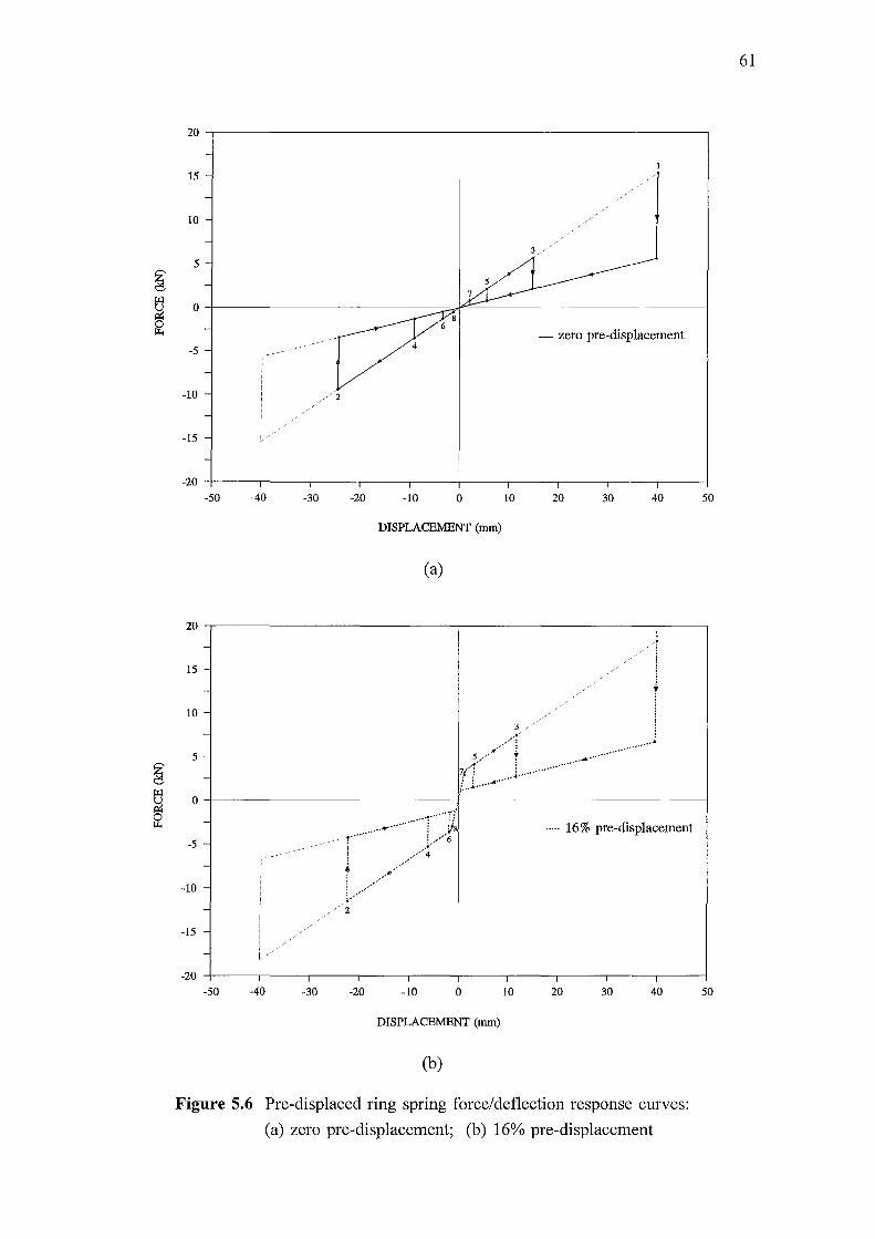
~ ~ 0 ~
~ ~ ~
20
15
10
3 /
5
0
- zero pre-displacement -5
I I I I I
-10 I
//2 I I / I /
/ I / I /
I / /
I / /
-15 ~/
~0 4------.-----.-----r-----.-----+-----.-----.-----.-----.----~
-50 -40 -30 -20 -10 0 10 20 30 40 50
DISPLACEMENT (mm)
(a)
20 1
-15 -
/I
-10 -
- I 5- ................................
-
0- -~---------~ ----!--- ----- ---------f--------·
-5
-10
-
-15
I I I I I I I I I I I I I I / I / I//
.... ···c ~.:: r~ ..... 16% pre-displacement
/z
-20 ~----.-----.------.-----r-----+-----.-----.-----.-----.----~
-50 -40 -30 -20 -10 0 10 20 30 40
DISPLACEMENT (mm)
(b)
Figure 5.6 Pre-displaced ring spring force/deflection response curves:
(a) zero pre-displacenaent; (b) 16~ pre-displacenaent
50
61
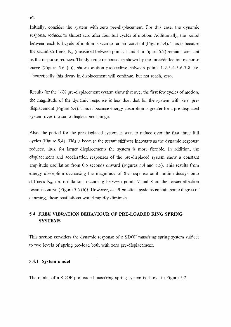
62
Initially, consider the system with zero pre-displacement. For this case, the dynamic
response reduces to almost zero after four full cycles of motion. Additionally, the period
between each full cycle of motion is seen to remain constant (Figure 5.4). This is because
the secant stiffness, Ki, (measured between points 1 and 3 in Figure 5.2) remains constant
as the response reduces. The dynamic response, as shown by the force/deflection response
curve (Figure 5.6 (a)), shows motion proceeding between points 1-2-3-4-5-6-7-8 etc.
Theoretically this decay in displacement will continue, but not reach, zero.
Results for the 16% pre-displacement system show that over the first few cycles of motion,
the magnitude of the dynamic response is less than that for the system with zero pre
displacement (Figure 5.4). This is because energy absorption is greater for a pre-displaced
system over the same displacement range.
Also, the period for the pre-displaced system is seen to reduce over the first three full
cycles (Figure 5.4). This is because the secant stiffness increases as the dynamic response
reduces, thus, for larger displacements the system is more flexible. In addition, the
displacement and acceleration responses of the pre-displaced system show a constant
amplitude oscillation from 0.5 seconds onward (Figures 5.4 and 5.5). This results from
energy absorption decreasing the magnitude of the response until motion decays onto
stiffness K0, i.e. oscillations occurring between points 7 and 8 on the force/deflection
response curve (Figure 5.6 (b)). However, as all practical systems contain some degree of
damping, these oscillations would rapidly diminish.
5.4 FREE VIBRATION BEHAVIOUR OF PRE-LOADED RING SPRING
SYSTEMS
This section considers the dynamic response of a SDOF mass/ring spring system subject
to two levels of spring pre-load both with zero pre-displacement.
5.4.1 System model
The model of a SDOF pre-loaded mass/ring spring system is shown in Figure 5.7.
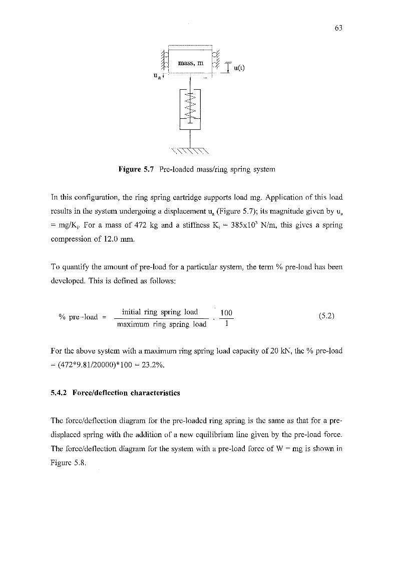
·········-----------------------., ' ' ' '
mass, m ::8 -f u(t) uar::··············T·------------~
Figure 5.7 Pre-loaded mass/ring spring system
63
In this configuration, the ring spring cartridge supports load mg. Application of this load
results in the system undergoing a displacement ua (Figure 5.7); its magnitude given by ua
= mg/Ki. For a mass of 472 kg and a stiffness Ki = 385x103 N/m, this gives a spring
compression of 12.0 mm.
To quantify the amount of pre-load for a particular system, the term% pre-load has been
developed. This is defined as follows:
% pre-load initial ring spring load
maximum ring spring load
100 1
(5.2)
For the above system with a maximum ring spring load capacity of 20 kN, the% pre-load
= (472*9.81/20000)*100 = 23.2%.
5.4.2 Force/deflection characteristics
The force/deflection diagram for the pre-loaded ring spring is the same as that for a pre
displaced spring with the addition of a new equilibrium line given by the pre-load force.
The force/deflection diagram for the system with a pre-load force of W = mg is shown in
Figure 5.8.
64
DEFLECTION
Figure 5.8 Force/deflection diagram for pre-loaded ring springs with
zero pre-displacement
5.4.3 Equation of motion
The generalised equation of motion for the free vibration of pre-loaded mass/ring spring
systems is:
mii + k*u = mg (5.3)
where k* and u(t) are as defined previously and mg is a constant force acting on the
system. This equation can be solved using the ring spring model computer algorithm.
5.4.4 Dynamic response
The free vibration response of a mass/ring spring system supporting weight mg (i.e. for
23.2% pre-load) and released from initial displacements of 40 mm and 15 mm was
determined. In addition, the response of a system with a 10% pre-load, released from an
initial displacement of 40 mm, was obtained. The displacement and acceleration responses
for these systems are presented in Figures 5.9 and 5.10, and their force/deflection response
curves are given in Figures 5.11 (a) and (b).
Discussion of the results for the pre-loaded systems follow.
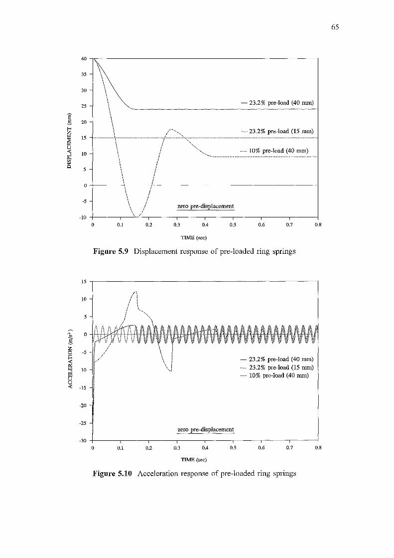
01
! ~
~ 5 a u ...::
40 ~------------------------------------------------------~
35
30
25
20 -
\ \
\ \ \
\ \
\
\ \
- 23.2% pre-load (40 mm)
\ /'·-.,., ····· 23.2% pre-load (15 mm) 15 - ................ \ .................................... / ........... ::-,,._<:~·-··········· .................................................................................. ..
\ / ·,, 10- \ I '·,·,·-·,·-·-·-·-·-·-----·-·-·-·-·::::: -~~-~--~:.:=~~~-~--~~?.- ~~---·-·
' ; i i
\ i I i
5 -
\ i \ i 0 -+----- ~~\\,,--------i,-------~----------------
\ i
zero pre-displacement \ I \ \ I
\ '
-5 -
-10 4------,,--·~\~,/-·-.------.------.------.-----~------.-----~
15
10
5
-5
-10
-15
-20
-25
-30
0 0.1 0.2 0.3 0.4 0.5 0.6 0.7
TIME (sec)
Figure 5.9 Displacement response of pre-loaded ring springs
zero pre-displacement
0 0.1 0.2 0.3 0.4 0.5
TIME (sec)
- 23.2% pre-load (40 mm) ..... 23.2% pre-load (15 mm) -·-·- 10% pre-load (40 mm)
0.6 0.7
Figure 5.10 Acceleration response of pre-loaded ring springs
0.8
0.8
65
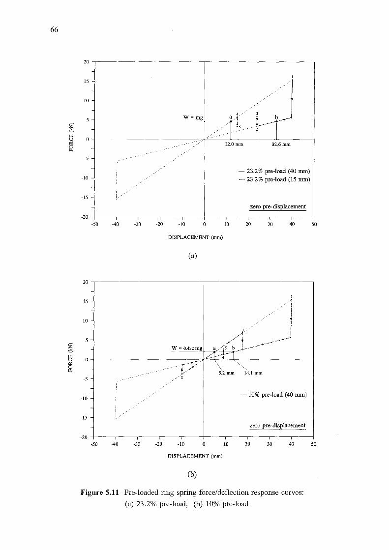
66
~ e:J ~ 0 ~
~ e:J ~ ~
20
-
15 -
10
5
-
0 ---------
-
-5 --
-10 -
-
-15 -
--20
-50
20
-
15 -
-
10-
-
5 -
-
0-
-
-5 -
-
-10 -
-
-15 -
-
-20
-50
/
I I I I I I I I I I I
I I !/
I
-40
I I I I I I I I I I I
I
--
/ /
I /
i/
-40
/ /
/ /
/ -/ ---/
/ /
/ /
/ /
/ /
/ /
I
-30
-30
/ / -
/ /
/ /
/ /
/ /
-20
-20
1 /
/ /
/ /
/ /
/ /
/ /
/ /
/ /
/ /
/ /
4/ 3 W=mg a/.; ; b
----------"-
< --- >l-~~------ 2
--
/ / /
/ ---;::/ 12.0 mm 32.6mm /
/ /
/
/ /
/ /
/ /
/ /
/ /
/
- 23.2% pre-load (40 mm) --· .. 23.2% pre-load (15 mm)
zero pre-displacement
I I I I
-10 0 10 20 30 40
DISPLACEMENT (rnm)
(a)
....... 10% pre-load (40 mm)
zero pre-displacement
-10 0 10 20 30 40
DISPLACEMENT (rnm)
(b)
Figure 5.11 Pre-loaded ring spring force/deflection response curves:
(a) 23.2% pre-load; (b) 10% pre-load
50
50
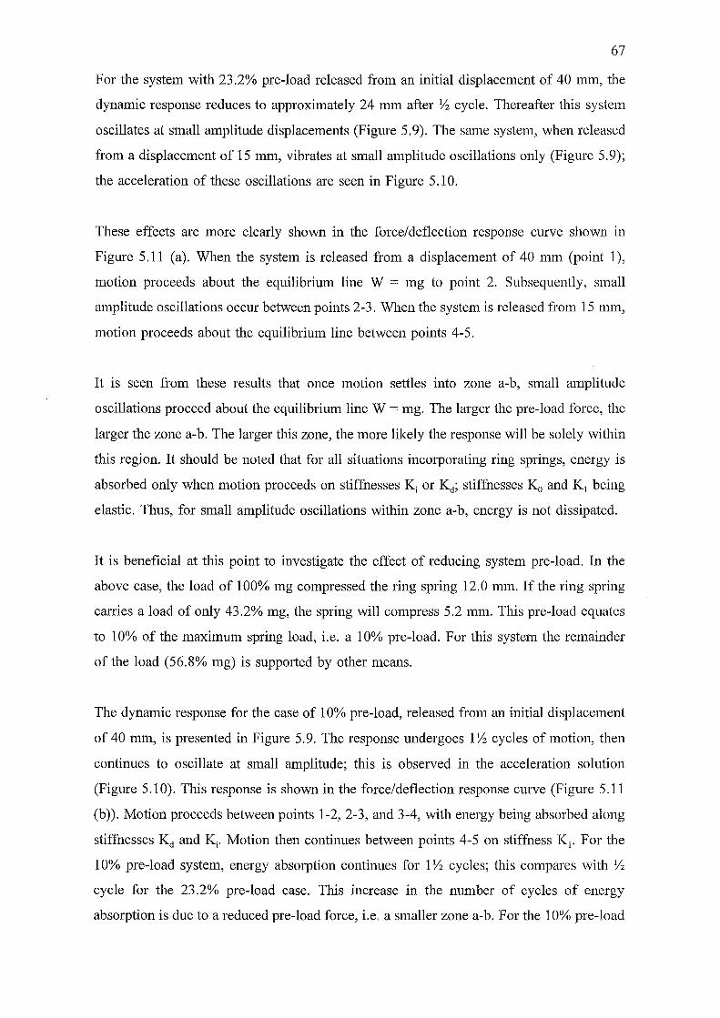
67
For the system with 23.2% pre-load released from an initial displacement of 40 mm, the
dynamic response reduces to approximately 24 mm after Yz cycle. Thereafter this system
oscillates at small amplitude displacements (Figure 5.9). The same system, when released
from a displacement of 15 mm, vibrates at small amplitude oscillations only (Figure 5.9);
the acceleration of these oscillations are seen in Figure 5.10.
These effects are more clearly shown in the force/deflection response curve shown in
Figure 5.11 (a). When the system is released from a displacement of 40 mm (point 1),
motion proceeds about the equilibrium line W = mg to point 2. Subsequently, small
amplitude oscillations occur between points 2-3. When the system is released from 15 mm,
motion proceeds about the equilibrium line between points 4-5.
It is seen from these results that once motion settles into zone a-b, small amplitude
oscillations proceed about the equilibrium line W = mg. The larger the pre-load force, the
larger the zone a-b. The larger this zone, the more likely the response will be solely within
this region. It should be noted that for all situations incorporating ring springs, energy is
absorbed only when motion proceeds on stiffnesses Ki or Kd; stiffnesses K 0 and K 1 being
elastic. Thus, for small amplitude oscillations within zone a-b, energy is not dissipated.
It is beneficial at this point to investigate the effect of reducing system pre-load. In the
above case, the load of 100% mg compressed the ring spring 12.0 mm. If the ring spring
carries a load of only 43.2% mg, the spring will compress 5.2 mm. This pre-load equates
to 10% of the maximum spring load, i.e. a 10% pre-load. For this system the remainder
of the load (56.8% mg) is supported by other means.
The dynamic response for the case of 10% pre-load, released from an initial displacement
of 40 mm, is presented in Figure 5.9. The response undergoes 1 Yz cycles of motion, then
continues to oscillate at small amplitude; this is observed in the acceleration solution
(Figure 5.10). This response is shown in the force/deflection response curve (Figure 5.11
(b)). Motion proceeds between points 1-2, 2-3, and 3-4, with energy being absorbed along
stiffnesses Kd and Ki. Motion then continues between points 4-5 on stiffness K 1• For the
10% pre-load system, energy absorption continues for 1 Yz cycles; this compares with Yz
cycle for the 23.2% pre-load case. This increase in the number of cycles of energy
absorption is due to a reduced pre-load force, i.e. a smaller zone a-b. For the 10% pre-load

68
case, zone a-b falls between 5.2 and 14.1 mm (Figure 5.11 (b)), this being much smaller
than the zone between 12.0 and 32.6 mm for 23.2% pre-load case (Figure 5.11(a)).
5.5 FREE VIBRATION BEHAVIOUR OF PRE-DISPLACED PRE-LOADED RING
SPRING SYSTEMS
This section details the dynamic response of a SDOF mass/ring spring system that is both
pre-displaced and pre-loaded. The system analysed is subjected to two levels of spring pre
load and has a pre-displacement of 16%.
5.5.1 System model
The model of a SDOF pre-displaced pre-loaded mass/ring spring system is shown in Figure
5.12.
mass, m =t; f u(t) u a r::: ______________ T _____________ ___r____1
Figure 5.12 Pre-displaced pre-loaded mass/ring spring system
In this system a pre-displaced ring spring cartridge supports load mg. For the case where
the total weight (1 00% mg) is carried by the cartridge, this equates to a pre-load of 23.2%
(as calculated in Section 5.4.1).
5.5.2 Force/deflection characteristics
The force/deflection diagram for a pre-displaced pre-loaded ring spring is the same as that
for a pre-displaced system with an equilibrium line given by the pre-load force. The
force/deflection diagram for the system with a pre-load of W = mg is shown in Figure
5.13.
DEFLECTION
Figure 5.13 Force/deflection diagram for pre-displaced pre-loaded ring springs
5.5.3 Equation of motion
The equation of motion for a pre-displaced pre-loaded system is given by:
mii + k*u = mg (5.4)
69
This equation is the same as that for a pre-loaded ring spring system with zero pre
displacement (Equation 5.3).
5.5.4 Dynamic response
The free vibration response of a mass/ring spring system of 16% pre-displacement and
23.2% pre-load, released from initial displacements of 40 mm and 15 mm, was computed.
Also analysed was a system with 10% pre-load released from a displacement of 40 mm.
The displacement and acceleration response for these systems are presented in Figures 5.14
and 5.15. Their force/deflection response curves are given in Figures 5.16 (a) and (b).
Results obtained for these pre-displaced pre-loaded systems are now discussed.
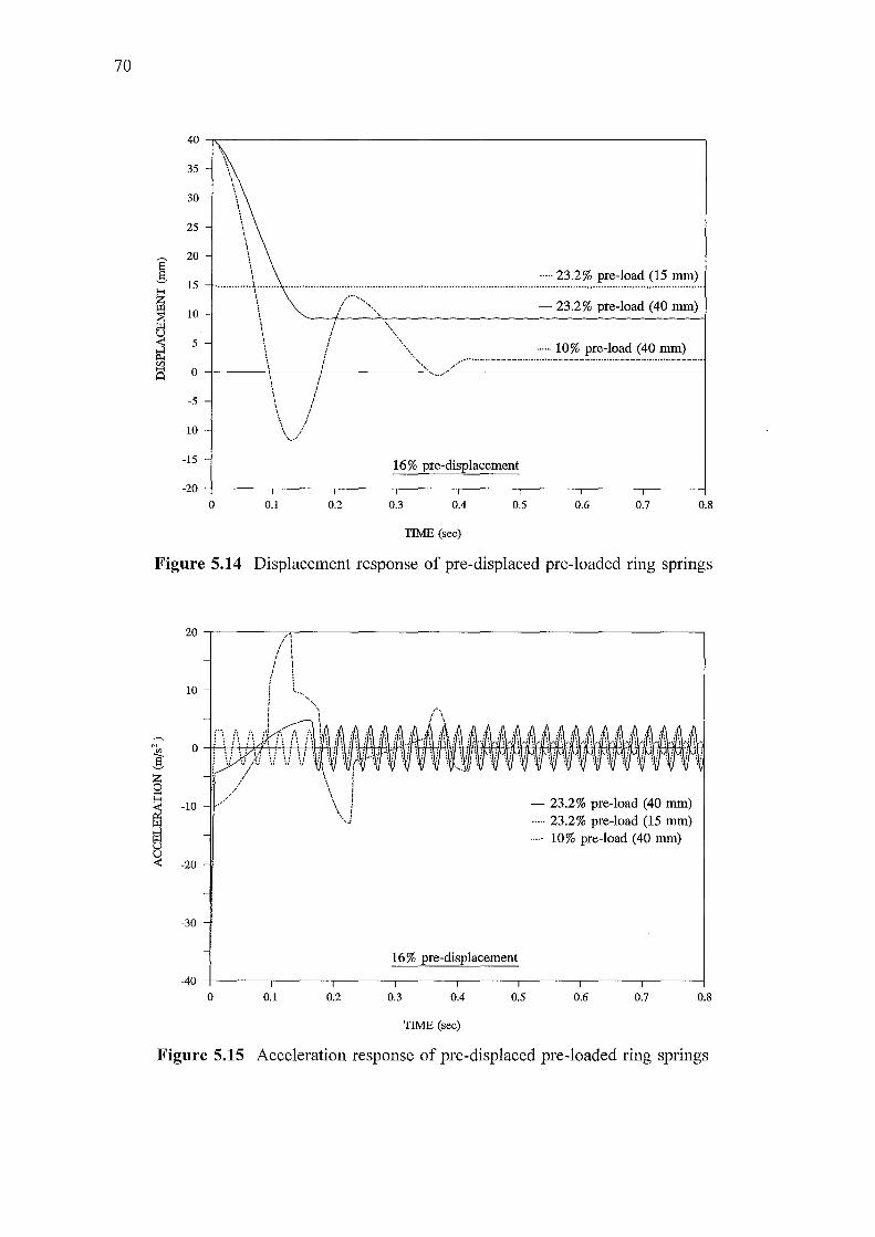
70
40
35 -
30 -
25 -
\ \
' \ \ ' ' ' ' \ \ \ ' ·, \
20 - \ \ \ ..... 23.2% pre-load (15 mm)
15 - ·············-\"""" .................................................................................................................................................. ..
10 \ /.-.,.,'.,, -23.2% pre-load (40 mm) \ i ·,. I i '\.
5 \ I ' . I ·,.. ---·-·- -·-·-·-·-·-·-·-·-·:::::.-~~~.-~~~=~~~.~-.~~?- ~~·-·-·-\ . '"·,, 0 -------\ J ,.-\ i
-5
-10
-15 -
\ I \ . \ / \ / ·-.../
16% pre-displacement
-20 +-----,---,-----,-----,----,----,------,------j
0 0.1 0.2 0.3 0.4 0.5 0.6 0.7 0.8
TIME (sec)
Figure 5.14 Displacement response of pre-displaced pre-loaded ring springs
i z 0
! u ~
20.-----,~ .. ---------------------~
10
0
/ /
-10 ·'
-20
-30
I !
/ I ! .
{
- 23.2% pre-load (40 mm) ...... 23.2% pre-load (15 mm) ·-- 10% pre-load (40 mm)
16% pre-displacement
-40 -+-----.----,------.------.----.-----.------.-----1 0 0.1 0.2 0.3 0.4 0.5 0.6 0.7 0.8
TIME (sec)
Figure 5.15 Acceleration response of pre-displaced pre-loaded ring springs
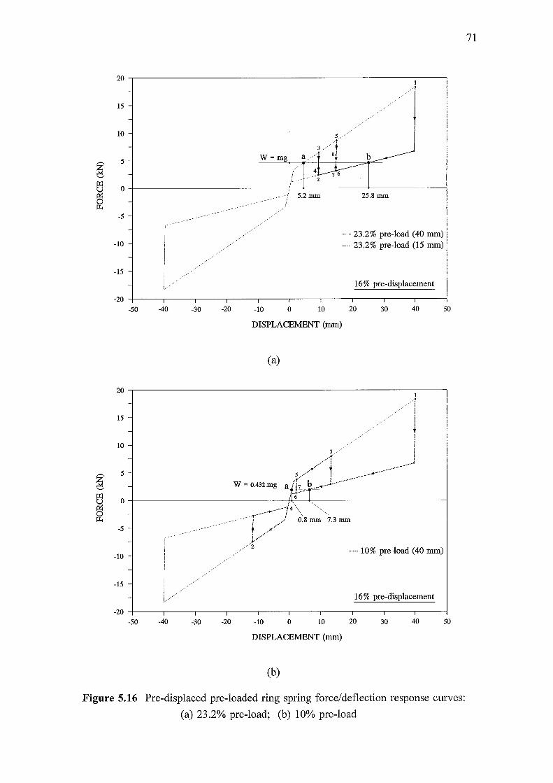
20
15
10
~ 5
~ 0
p:.
-5
-10
-15
-20
-50 -40 -30
20
-
15 -
-
10 -
-
~ 5 -
-
~ 0
-p:.
-5 -
r - I I I
-10 - I I I I - I I I
-15 - I I I I /
- I / 1//
-20
-50 -40 -30
-20 -10 0 10
DISPLACEMENT (nun)
(a)
-20 -10 0 10
DISPLACEMENT (nun)
(b)
-23.2% pre-load (40 nun) ····· 23.2% pre-load (15 nun)
16% pre-displacement
20
/ /
/
30 40
1
/ /1 i ! ! t I i ........
-·-.. 10% pre-load (40 nun)
16% pre-displacement
20 30 40
50
50
Figure 5.16 Pre-displaced pre-loaded ring spring force/deflection response curves:
(a) 23.2% pre-load; (b) 10% pre-load
71
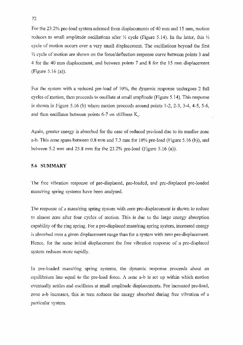
72
For the 23.2% pre-load system released from displacements of 40 mm and 15 mm, motion
reduces to small amplitude oscillations after Yz cycle (Figure 5.14). In the latter, this Yz
cycle of motion occurs over a very small displacement. The oscillations beyond the first
Yz cycle of motion are shown on the force/deflection response curve between points 3 and
4 for the 40 mm displacement, and between points 7 and 8 for the 15 mm displacement
(Figure 5. 16 (a)).
For the system with a reduced pre-load of 10%, the dynamic response undergoes 2 full
cycles of motion, then proceeds to oscillate at small amplitude (Figure 5.14). This response
is shown in Figure 5.16 (b) where motion proceeds around points 1-2, 2-3, 3-4, 4-5, 5-6,
and then oscillates between points 6-7 on stiffness K1•
Again, greater energy is absorbed for the case of reduced pre-load due to its smaller zone
a-b. This zone spans between 0.8 mm and 7.3 mm for 10% pre-load (Figure 5.16 (b)), and
between 5.2 mm and 25.8 mm for the 23.2% pre-load (Figure 5.16 (a)).
5.6 SUMMARY
The free vibration response of pre-displaced, pre-loaded, and pre-displaced pre-loaded
mass/ring spring systems have been analysed.
The response of a mass/ring spring system with zero pre-displacement is shown to reduce
to almost zero after four cycles of motion. This is due to the large energy absorption
capability of the ring spring. For a pre-displaced mass/ring spring system, increased energy
is absorbed over a given displacement range than for a system with zero pre-displacement.
Hence, for the same initial displacement the free vibration response of a pre-displaced
system reduces more rapidly.
In pre-loaded mass/ring spring systems, the dynamic response proceeds about an
equilibrium line equal to the pre-load force. A zone a-b is set up within which motion
eventually settles and oscillates at small amplitude displacements. For increased pre-load,
zone a-b increases, this in turn reduces the energy absorbed during free vibration of a
particular system.

Chapter 6
DYNAMIC TESTING OF A PRE-DISPLACED MASS/RING
SPRING CARTRIDGE SYSTEM: COMPARISON WITH
COMPUTER SIMULATION RESULTS
6.1 INTRODUCTION
73
Computer analyses provide a powerful tool for determining the response of structural
systems subject to dynamic excitation. However, it is important that their accuracy be
determined by comparing results with those given by experimental testing. This chapter
details results of experimental testing of a mass/ring spring system subject to short duration
excitation. The system comprises of a ring spring cartridge (detailed in Chapter 4) attached
to a rigid mass and mounted on a shaker table. Shaker table test results for spring pre
displacements of 16% and 28% are presented. These results are then compared with those
given by computer simulation.
6.2 EXPERIMENTAL SYSTEM
To enable the dynamic behaviour of mass/ring spnng systems to be analysed
experimentally, a test assembly was built and subsequently tested (Hill1995c ). This system
is now detailed.
6.2.1 Mass/ring spring cartridge system
The experimental system comprises of a bi-directional ring spring cartridge attached to a
mass, m, and mounted on a shaker as shown in Figure 6.1.
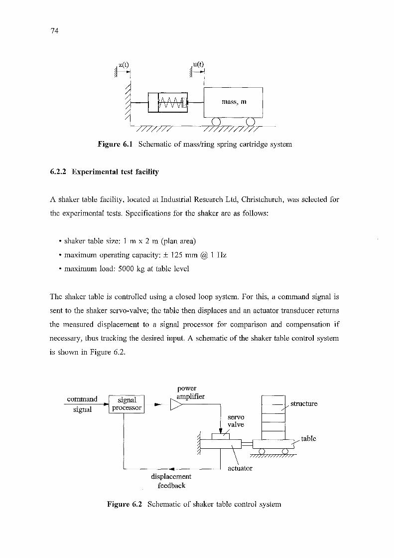
74
mass, m
Figure 6.1 Schematic of mass/ring spring cartridge system
6.2.2 Experimental test facility
A shaker table facility, located at Industrial Research Ltd, Christchurch, was selected for
the experimental tests. Specifications for the shaker are as follows:
• shaker table size: 1 m x 2 m (plan area)
• maximum operating capacity: ± 125 mm @ 1 Hz
• maximum load: 5000 kg at table level
The shaker table is controlled using a closed loop system. For this, a command signal is
sent to the shaker servo-valve; the table then displaces and an actuator transducer returns
the measured displacement to a signal processor for comparison and compensation if
necessary, thus tracking the desired input. A schematic of the shaker table control system
is shown in Figure 6.2.
command
signal
power amplifier
displacement feedback
actuator
Figure 6.2 Schematic of shaker table control system
structure
table
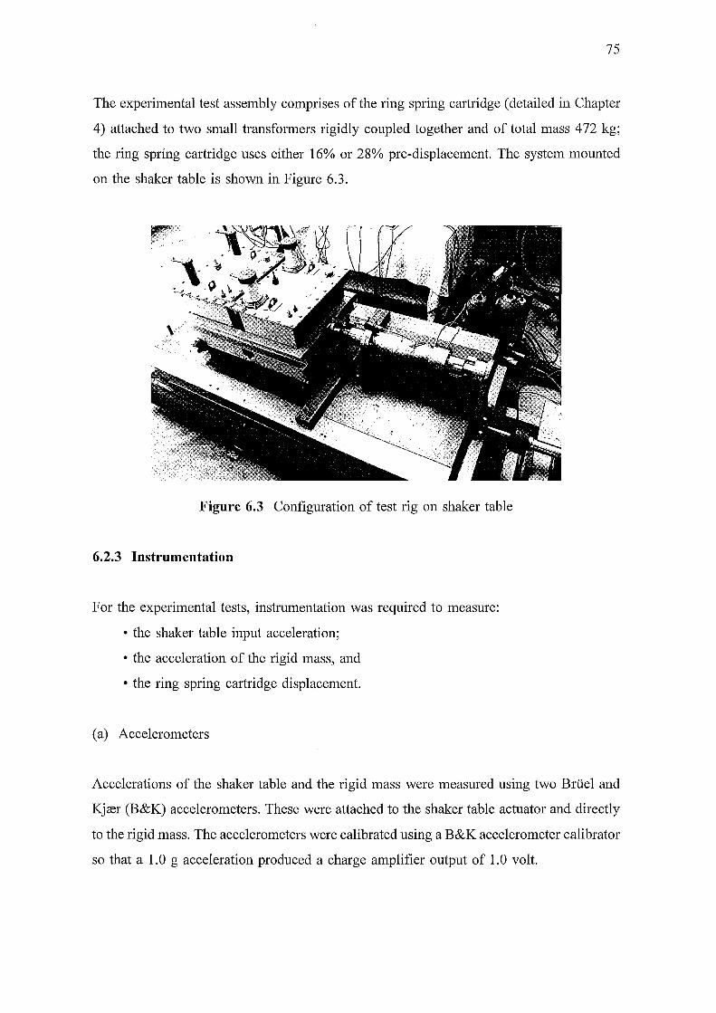
75
The experimental test assembly comprises of the ring spring cartridge (detailed in Chapter
4) attached to two small transformers rigidly coupled together and of total mass 472 kg;
the ring spring cartridge uses either 16% or 28% pre-displacement. The system mounted
on the shaker table is shown in Figure 6.3.
Figure 6.3 Configuration of test rig on shaker table
6.2.3 Instrumentation
For the experimental tests, instrumentation was required to measure:
• the shaker table input acceleration;
• the acceleration of the rigid mass, and
• the ring spring cartridge displacement.
(a) Accelerometers
Accelerations of the shaker table and the rigid mass were measured using two Briiel and
Kj<er (B&K) accelerometers. These were attached to the shaker table actuator and directly
to the rigid mass. The accelerometers were calibrated using a B&K accelerometer calibrator
so that a 1.0 g acceleration produced a charge amplifier output of 1.0 volt.
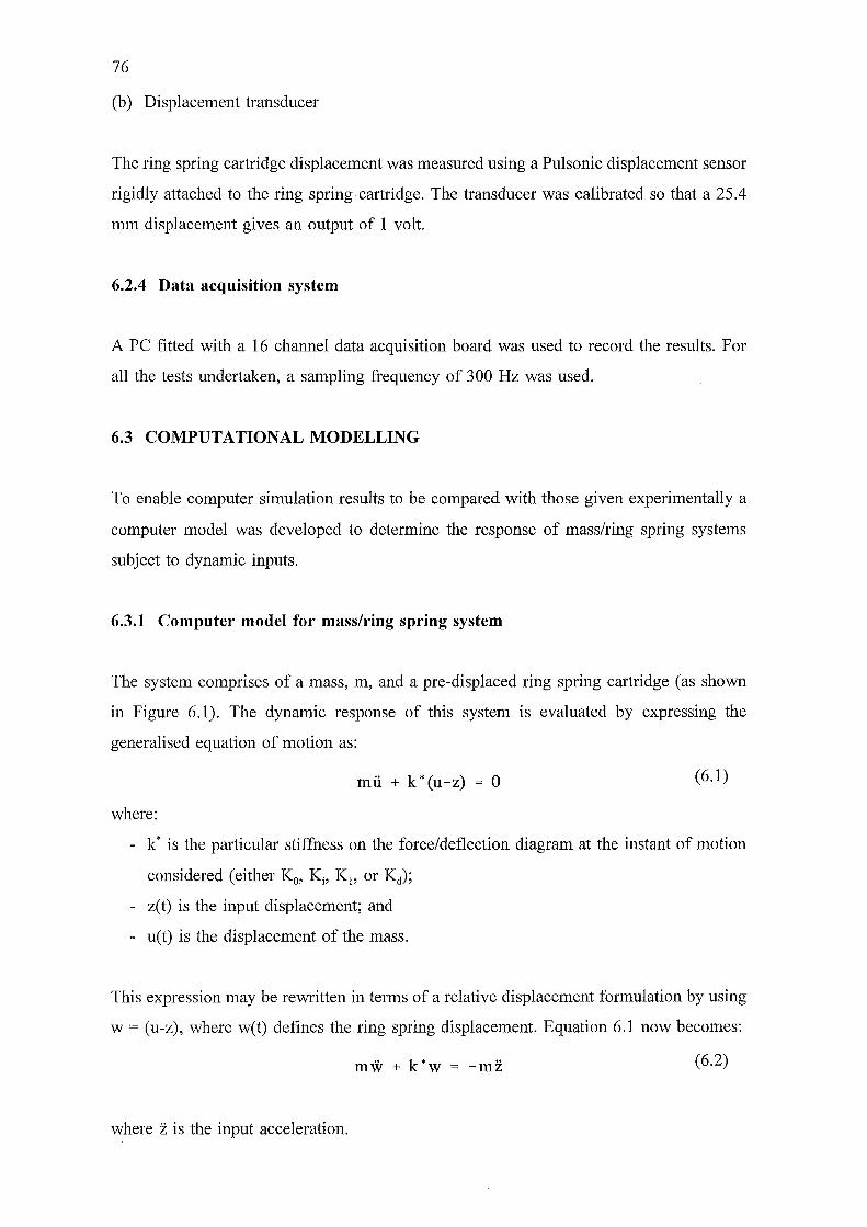
76
(b) Displacement transducer
The ring spring cartridge displacement was measured using a Pulsonic displacement sensor
rigidly attached to the ring spring cartridge. The transducer was calibrated so that a 25.4
mm displacement gives an output of 1 volt.
6.2.4 Data acquisition system
A PC fitted with a 16 channel data acquisition board was used to record the results. For
all the tests undertaken, a sampling frequency of 300 Hz was used.
6.3 COMPUTATIONAL MODELLING
To enable computer simulation results to be compared with those given experimentally a
computer model was developed to determine the response of mass/ring spring systems
subject to dynamic inputs.
6.3.1 Computer model for mass/ring spring system
The system comprises of a mass, m, and a pre-displaced ring spring cartridge (as shown
in Figure 6.1). The dynamic response of this system is evaluated by expressing the
generalised equation of motion as:
mii + k*(u-z) = 0 (6.1)
where:
- k* is the particular stiffness on the force/deflection diagram at the instant of motion
considered (either K 0, Ki, K 1, or Kd);
- z(t) is the input displacement; and
- u(t) is the displacement of the mass.
This expression may be rewritten in terms of a relative displacement formulation by using
w = (u-z), where w(t) defines the ring spring displacement. Equation 6.1 now becomes:
mw + k*w = -mz (6.2)
where z is the input acceleration.
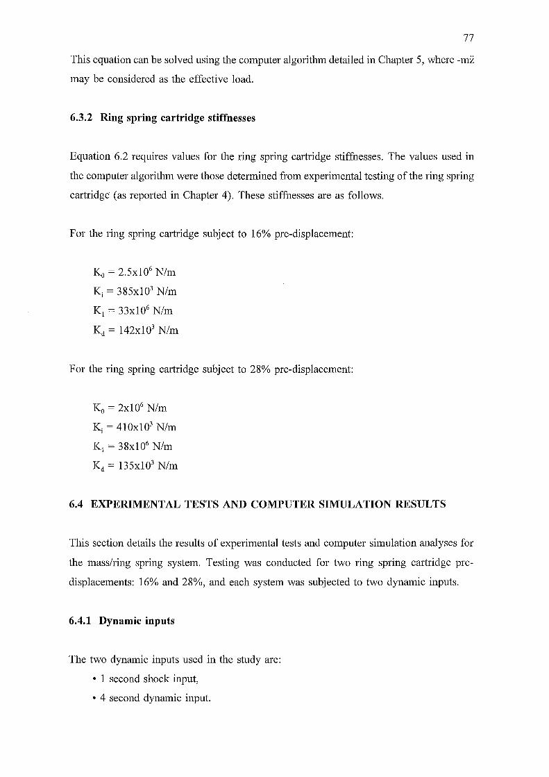
77
This equation can be solved using the computer algorithm detailed in Chapter 5, where -mz
may be considered as the effective load.
6.3.2 Ring spring cartridge stiffnesses
Equation 6.2 requires values for the ring spring cartridge stiffnesses. The values used in
the computer algorithm were those determined from experimental testing of the ring spring
cartridge (as reported in Chapter 4). These stiffnesses are as follows.
For the ring spring cartridge subject to 16% pre-displacement:
K0 = 2.5xl06 N/m
Ki = 385xl03 N/m
K1 = 33xl06 N/m
Kd = 142x103 N/m
For the ring spring cartridge subject to 28% pre-displacement:
K0 = 2xl06 N/m
Ki = 410xl03 N/m
K1 = 38xl06 N/m
Kd = 135x103 N/m
6.4 EXPERIMENTAL TESTS AND COMPUTER SIMULATION RESULTS
This section details the results of experimental tests and computer simulation analyses for
the mass/ring spring system. Testing was conducted for two ring spring cmiridge pre
displacements: 16% and 28%, and each system was subjected to two dynamic inputs.
6.4.1 Dynamic inputs
The two dynamic inputs used in the study are:
• 1 second shock input,
• 4 second dynamic input.

78
The 1 second shock input was generated by manually controlling the shaker table
displacement using a hand-held potentiometer. Different signals were obtained for the 16%
and 28% pre-displaced systems.
The 4 second dynamic input was obtained using a signal derived from the first 12 seconds
of the Pacoima 1971 S16E earthquake (this earthquake is detailed in Chapter 7). The
emihquake acceleration was trebled and its time base reduced by a factor of three to give
the desired short duration excitation, i.e., from a 12 second record to a 4 second record.
This signal was then used as the shaker table input for the 16% and 28% pre-displaced
systems, thus enabling these experimental results to be compared for the same input.
The measured shaker table accelerations were used as the computer algorithm inputs to
enable experimental and computational results to be compared for the same excitation.
6.4.2 Dynamic response of system subjected to 1 second input
(a) 16% pre-displacement
The graphical results presented for the 16% pre-displaced system subjected to the 1 second
shock input are:
• recorded shaker table input acceleration (Figure 6.4)
• ring spring cartridge displacement - experimental and computational (Figure 6.5)
• acceleration of the mass - experimental and computational (Figure 6.6)
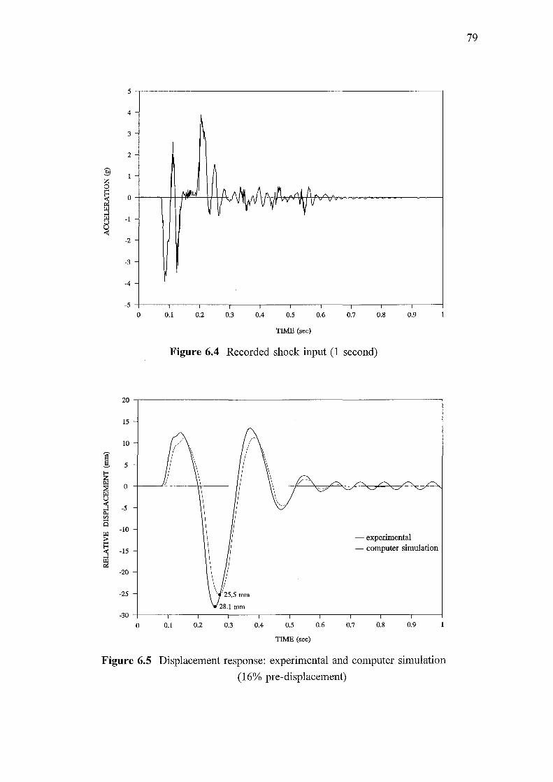
5
4
3
2
3 z 0 ~ 0
~ 0 -1
~ -2
-3
-4
-5 0
20
15
10
I 5
!i
~ 0
< ~ -5 </.) ...... Q
-10
~ -15
~ -20
-25
-30
0
Figure 6.5
0.1 0.2 0.3 0.4 0.5 0.6 0.7 0.8 0.9
TIME (sec)
Figure 6.4 Recorded shock input (1 second)
0.1 0.2 0.3 0.4 0.5
TIME (sec)
- experimental - computer simulation
0.6 0.7 0.8 0.9
1
Displacement response: experimental and computer simulation
( 16% pre-displacement)
79
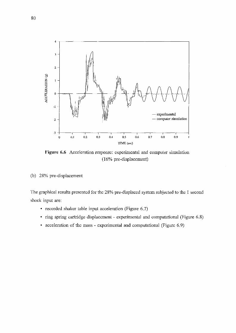
80
4,-------------------------------------------------~
3
2
-1
- experimental
-2 - computer simulation
-3 ,_---,----,----,,---,----,,----.----.----.----.---~
0 0.1 0.2 0.3 0.4 0.5 0.6 0.7 0.8 0.9
TIME (sec)
Figure 6.6 Acceleration response: experimental and computer simulation
( 16% pre-displacement)
(b) 28% pre-displacement
The graphical results presented for the 28% pre-displaced system subjected to the 1 second
shock input are:
• recorded shaker table input acceleration (Figure 6. 7)
• ring spring cartridge displacement - experimental and computational (Figure 6.8)
• acceleration of the mass - experimental and computational (Figure 6.9)
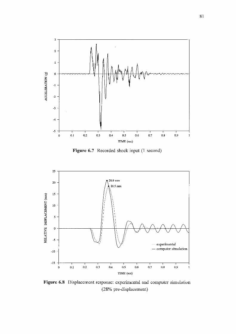
3
2 -
-
§ 0
5 ~ -1
~ El -2 ~
-
-
-3
-4
-5
0
25
20
I 15
I 10
j ~
5 rJ) ...... 0
~ 0
~ -5
-10
-15
0
Figure 6.8
0.1 0.2 0.3
A A '~ N A ~ ¥\ IL~ v v v I \J v v
0.4 0.5
TIME (sec)
0.6 0.7
¥
0.8 0.9
Figure 6. 7 Recorded shock input ( 1 second)
0.1 0.2 0.3 0.4 0.5
TIME (sec)
0.6
- experimental - computer simulation
0.7 0.8 0.9
Displacement response: experimental and computer simulation
(28% pre-displacement)
81
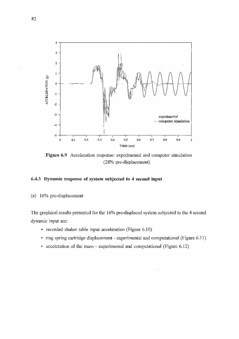
82
4
3
2
:§ z 0 0 b1
~ -1 tl u u ~ -2
-3
-4
-5
0
Figure 6.9
- experimental - computer simulation
0.1 0.2 0.3 0.4 0.5 0.6 0.7 0.8 0.9
TIME (sec)
Acceleration response: experimental and computer simulation
(28% pre-displacement)
6.4.3 Dynamic response of system subjected to 4 second input
(a) 16% pre-displacement
The graphical results presented for the 16% pre-displaced system subjected to the 4 second
dynamic input are:
• recorded shaker table input acceleration (Figure 6.1 0)
• ring spring cartridge displacement - experimental and computational (Figure 6.11)
• acceleration of the mass - experimental and computational (Figure 6.12)
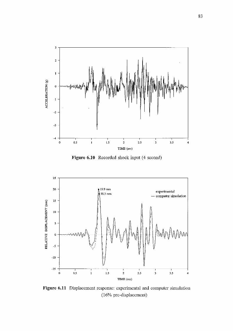
:§
~ 0
~ -1
~ -2
-3
-4
0
25
20
I 15
!i 10
8 j 5 p., rJ) ..... A
~ 0
~ gj -5
-10
-15
0
0.5 1.5 2 2.5 3 3.5
TIME (sec)
Figure 6.10 Recorded shock input ( 4 second)
0.5
19.9mm
18.3 rum
1.5 2
TIME (sec)
2.5
- experimental - computer simulation
3 3.5
4
4
Figure 6.11 Displacement response: experimental and computer simulation
(16% pre-displacement)
83
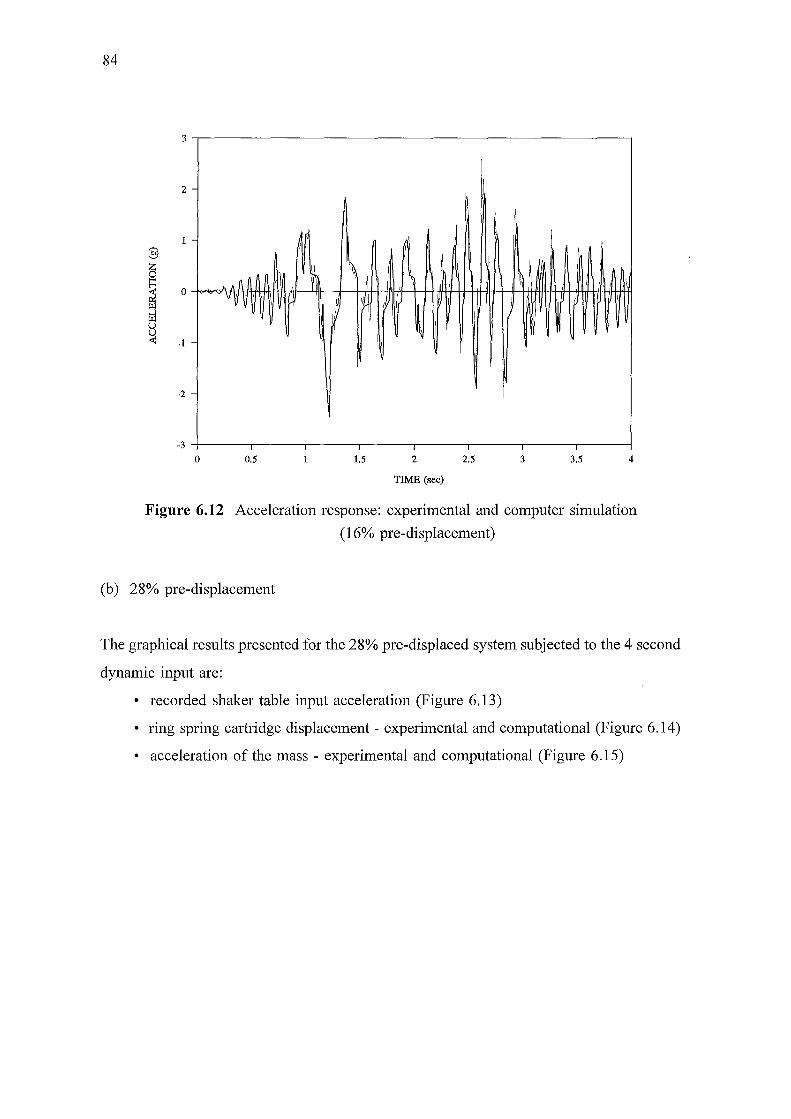
84
3.-----------------------------------------------~
2
0
-1
-2 -
-3~----------------~----~-----.-----.-----.----~
0 0.5 1.5 2
TIME (sec)
2.5 3 3.5 4
Figure 6.12 Acceleration response: experimental and computer simulation
( 16% pre-displacement)
(b) 28% pre-displacement
The graphical results presented for the 28% pre-displaced system subjected to the 4 second
dynamic input are:
• recorded shaker table input acceleration (Figure 6.13)
• ring spring cartridge displacement- experimental and computational (Figure 6.14)
• acceleration of the mass - experimental and computational (Figure 6 .15)
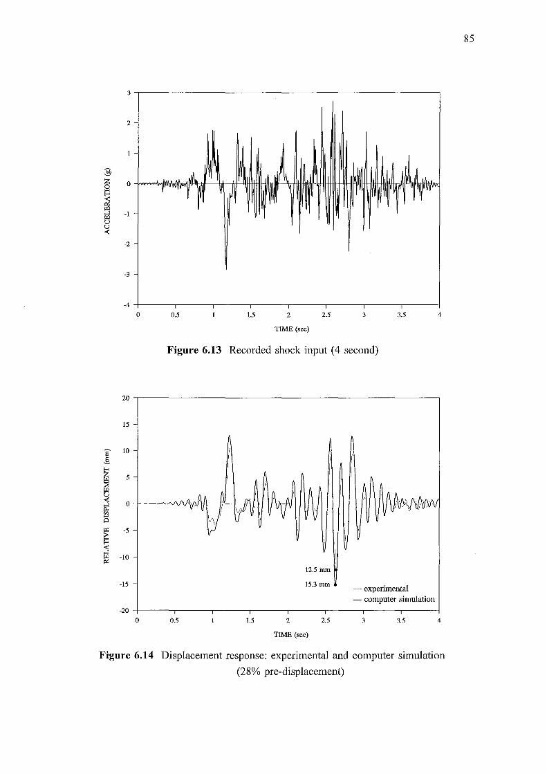
3
2
1
:§
~ 0
~ 0 -1 -
u <
-2 -
-3 -
-4
0
20
15
I 10
~ El
5
~ 0 til >-< A
~ -5
j g;J -10
-15
-20
0
.hi .~.~ v· ,,..f·~ ~ J\ ~
0.5 1.5
~~
2
TIME (sec)
2.5
~~ ''II
3
~ .lA rr 1~'VV'
3.5
Figure 6.13 Recorded shock input ( 4 second)
0.5 1.5
\ '
12.5 mm
15.3 mm
2
TIME (sec)
2.5
-··- experimental - computer simulation
3 3.5
4
4
Figure 6.14 Displacement response: experimental and computer simulation
(28% pre-displacement)
85
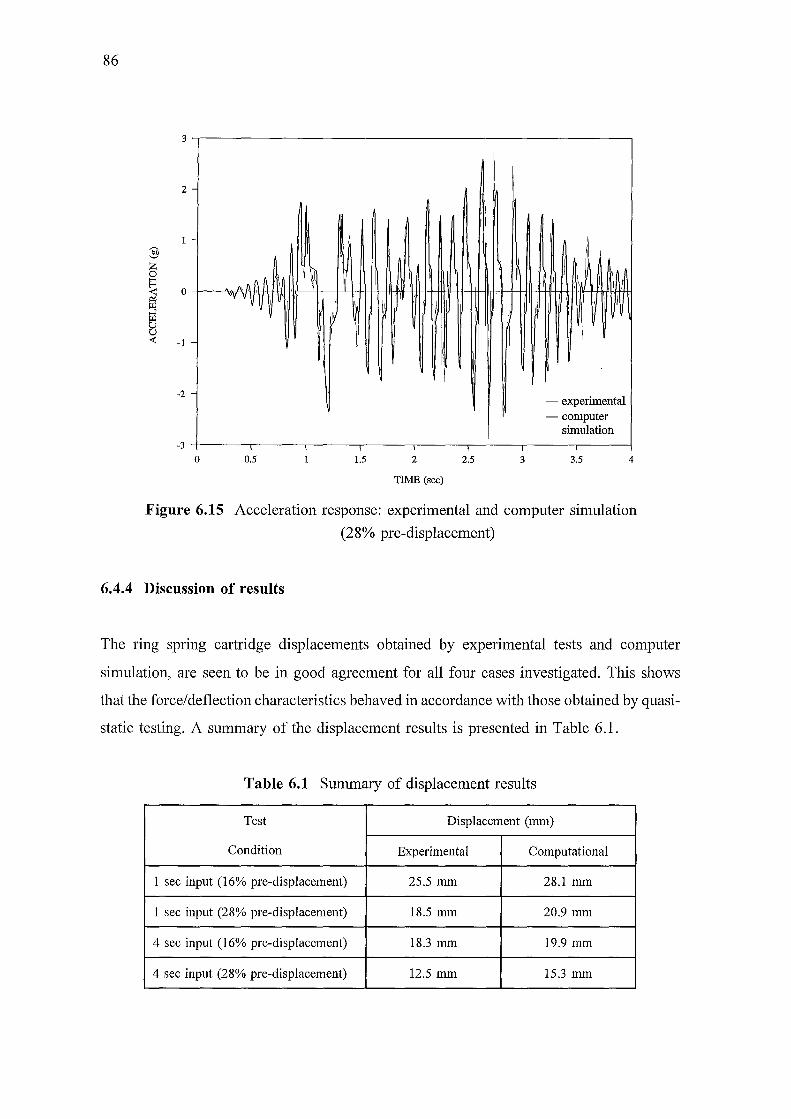
86
3,---------------------------------------------------~
2-
I I J ~ I II '\ -1-t-t+-iHI-f\!Hti+ 11---l--tt/--ttttc-l-t-+-lil--1
i :I; I I I I J' 1
-1
-2 -- experimental -computer
simulation -3 ~----------~------~----~----~------~----~----~
0 0.5 1.5 2
TIME (sec)
2.5 3 3.5 4
Figure 6.15 Acceleration response: experimental and computer simulation
(28% pre-displacement)
6.4.4 Discussion of results
The ring spring cartridge displacements obtained by experimental tests and computer
simulation, are seen to be in good agreement for all four cases investigated. This shows
that the force/deflection characteristics behaved in accordance with those obtained by quasi
static testing. A summary of the displacement results is presented in Table 6.1.
Table 6.1 Summary of displacement results
Test Displacement (mm)
Condition Experimental Computational
1 sec input (16% pre-displacement) 25.5 mm 28.1 mm
1 sec input (28% pre-displacement) 18.5 mm 20.9 mm
4 sec input (16% pre-displacement) 18.3 mm 19.9 mm
4 sec input (28% pre-displacement) 12.5 mm 15.3 mm
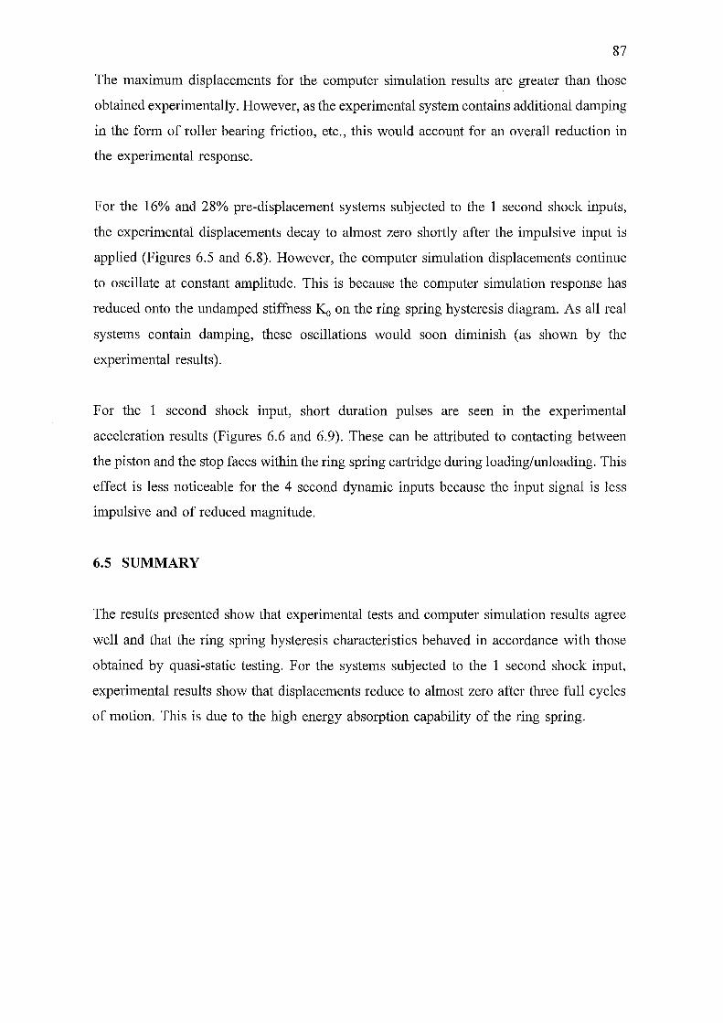
87
The maximum displacements for the computer simulation results are greater than those
obtained experimentally. However, as the experimental system contains additional damping
in the form of roller bearing friction, etc., this would account for an overall reduction in
the experimental response.
For the 16% and 28% pre-displacement systems subjected to the 1 second shock inputs,
the experimental displacements decay to almost zero shortly after the impulsive input is
applied (Figures 6.5 and 6.8). However, the computer simulation displacements continue
to oscillate at constant amplitude. This is because the computer simulation response has
reduced onto the undamped stiffness Ko on the ring spring hysteresis diagram. As all real
systems contain damping, these oscillations would soon diminish (as shown by the
experimental results).
For the 1 second shock input, short duration pulses are seen in the experimental
acceleration results (Figures 6.6 and 6.9). These can be attributed to contacting between
the piston and the stop faces within the ring spring cartridge during loading/unloading. This
effect is less noticeable for the 4 second dynamic inputs because the input signal is less
impulsive and of reduced magnitude.
6.5 SUMMARY
The results presented show that experimental tests and computer simulation results agree
well and that the ring spring hysteresis characteristics behaved in accordance with those
obtained by quasi-static testing. For the systems subjected to the 1 second shock input,
experimental results show that displacements reduce to almost zero after three full cycles
of motion. This is due to the high energy absorption capability of the ring spring.

88

Chapter 7
EARTHQUAKE-RESISTANT DESIGN
UTILISING RING SPRINGS
7.1 INTRODUCTION
89
The investigation to date has detailed the characteristics and dynamic behaviour of ring
spring systems. Based on these characteristics, ring springs would appear suitable
candidates for use in situations requiring additional flexibility as well as damping
capability.
This chapter considers practical applications in which ring springs may be employed. One
application identified as being particularly promising, is in utilising ring springs in seismic
isolation systems. The benefits of utilising ring springs in these applications are discussed.
Further, an innovative isolation system that aims to reduce the level of dynamic loading
experienced by a structure during an earthquake, has been developed. This system is
detailed, followed by computer analyses undertaken to establish the efficacy of the design.
A summary of the results of these analyses is presented.
7.2 EARTHQUAKE-RESISTANT DESIGN
In the design of structures located in regions of seismic risk, it is imperative that the
influence of earthquake generated forces be considered. In Chapter 2, the earthquake
resistant design techniques, along with numerous devices developed for use within
earthquake-resistant structures, were reported. The following sections investigate the
possibility of utilising ring springs in earthquake-resistant systems.
7.2.1 Seismic isolation systems utilising ring springs
As reported in Chapter 2, ring springs have been suggested for use as seismic energy
dissipaters (Shepherd and Erasmus, 1988; Erasmus 1988). In addition, Hill (1995d)
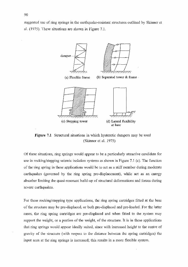
90
suggested use of ring springs in the earthquake-resistant structures outlined by Skinner et
al. (1975). These situations are shown in Figure 7.1.
damper
(a) Flexible frame
(c) Stepping tower
(b) Separated tower & frame
(d) Lateral flexibility at base
Figure 7.1 Structural situations in which hysteretic dampers may be used
(Skinner et al. 1975)
Of these situations, ring springs would appear to be a particularly attractive candidate for
use in rocking/stepping seismic isolation systems as shown in Figure 7.1 (c). The function
of the ring spring in these applications would be to act as a stiff member during moderate
earthquakes (governed by the ring spring pre-displacement), while act as an energy
absorber limiting the quasi-resonant build-up of structural deformations and forces during
severe earthquakes.
For these rocking/stepping type applications, the ring spring cartridges fitted at the base
of the structure may be pre-displaced, or both pre-displaced and pre-loaded. For the latter
cases, the ring spring cartridges are pre-displaced and when fitted to the system may
support the weight, or a portion of the weight, of the structure. It is in these applications
that ring springs would appear ideally suited, since with increased height to the centre of
gravity of the structure (with respect to the distance between the spring cartridges) the
input seen at the ring springs is increased; this results in a more flexible system.
91
7.2.2 Potential benefits of ring springs
The potential benefits of utilising ring springs in seismic isolation systems are (Hill1995d):
both the dissipative mechanism (friction) and system flexibility (spring) are
incorporated within a single unit;
ring springs remain fully elastic throughout the seismic disturbance - replacement
after a major earthquake is not necessary thus providing protection against
aftershocks;
the elastic restoring force relocates the structure near to its original position;
spring pre-tension may be adjusted such that sufficient rigidity exists to resist
service loadings (such as wind and small earthquakes);
minimal or no maintenance is required;
a wide range of loading situations is possible as ring springs are commercially
available in load carrying capacities ranging from 5 kN to 10 000 kN.
7.2.3 Practical applications for use of ring springs
Columnar type structures are those primarily suited to rocking/stepping systems. Possible
candidates include multi-storey buildings, chimneys, towers, as well as other similarly
proportioned structures.
An application for which ring springs would appear to be suitable is in protecting high
voltage electrical equipment during earthquakes. A number of features specific to high
voltage electrical equipment make it necessary to provide these items with adequate
protection from seismic damage. First, it is generally considered that electricity supply is
essential after a major earthquake, therefore, electrical equipment should be designed to
withstand a maximum design level earthquake. In addition, many items of electrical
equipment possess fundamental periods in the range 0.125-0.5 seconds and thereby
experience acceleration amplification during earthquakes with dominant periods in this
range. Also, high voltage electrical equipment of necessity requires adequate electrical
insulation from the ground and surrounding structures, thus, many items incorporate brittle
insulating members which are highly susceptible to fracture and possess little inherent
damping. Typical damping factors of2% are common for high voltage electrical equipment

92
(Pham and Hoby 1991), however, structural damping as low as 0.8% of critical has been
measured for some items (Rutledge et al. 1984).
The susceptibility of high voltage electrical equipment has been demonstrated by damage
sustained during only moderately sized earthquakes. The San Fernando earthquake on 9
February 1971 of magnitude 6.6, caused damage totalling $30 million to a new $110
million electrical converter station; circuit breakers were reported as being especially
vulnerable (Hausner and Jennings 1972). In New Zealand, an earthquake 9 km north of
the Tokaanu Power Station on 5 March 1984 of magnitude 5.6, caused damage to 5 out
of 33 current transformers, and 10 out of 12 capacitor voltage transformers broke at their
base (Rutledge et al. 1984). An earthquake near Edgecumbe in the North Island of New
Zealand, on 2 March 1987 of magnitude 6.3, caused extensive damage to buswork,
transformers and circuit breakers at the Edgecumbe and Kawerau Substations (Pender and
Robertson 1987; Rutledge 1988).
Work undertaken in New Zealand since the late 1960's has considered methods of
protecting items of high voltage electrical equipment during earthquakes (Hitchcock 1969,
Hitchcock 1973). This has lead to the development and installation of several isolation
systems (Pham 1988; Safi et al. 1989; Cousins et al. 1991; Coad and Pham 1993).
Recently, Pham reported on the use of Belleville washers in protecting such equipment
(Pham and Hoby 1991). The system developed utilises Belleville washers fitted between
the item of equipment and its support stand, thus increasing system flexibility and
damping. Tests carried out on a Belleville washer damper gave a damping factor of 4.4%,
with site tests conducted on three items of electrical equipment fitted with dampers giving
an average increase in damping of 4.1% (Pham and Hoby 1991). Ring springs, with
damping factors as high as 17.6% (Hill 1994b), could provide these items with increased
seismic protection.
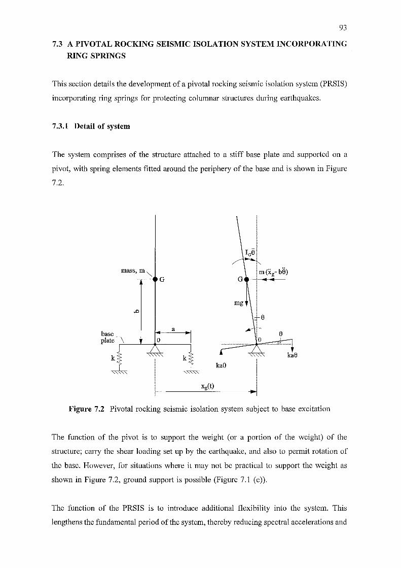
93
7.3 A PIVOTAL ROCKING SEISMIC ISOLATION SYSTEM INCORPORATING
RING SPRINGS
This section details the development of a pivotal rocking seismic isolation system (PRSIS)
incorporating ring springs for protecting columnar structures during earthquakes.
7.3.1 Detail of system
The system comprises of the structure attached to a stiff base plate and supported on a
pivot, with spring elements fitted around the periphery of the base and is shown in Figure
7.2.
mass, m"'-G
Xg(t)
kae
I
...1
Figure 7.2 Pivotal rocking seismic isolation system subject to base excitation
The function of the pivot is to support the weight (or a portion of the weight) of the
structure; carry the shear loading set up by the earthquake, and also to permit rotation of
the base. However, for situations where it may not be practical to suppmi the weight as
shown in Figure 7 .2, ground support is possible (Figure 7.1 (c)).
The function of the PRSIS is to introduce additional flexibility into the system. This
lengthens the fundamental period of the system, thereby reducing spectral accelerations and
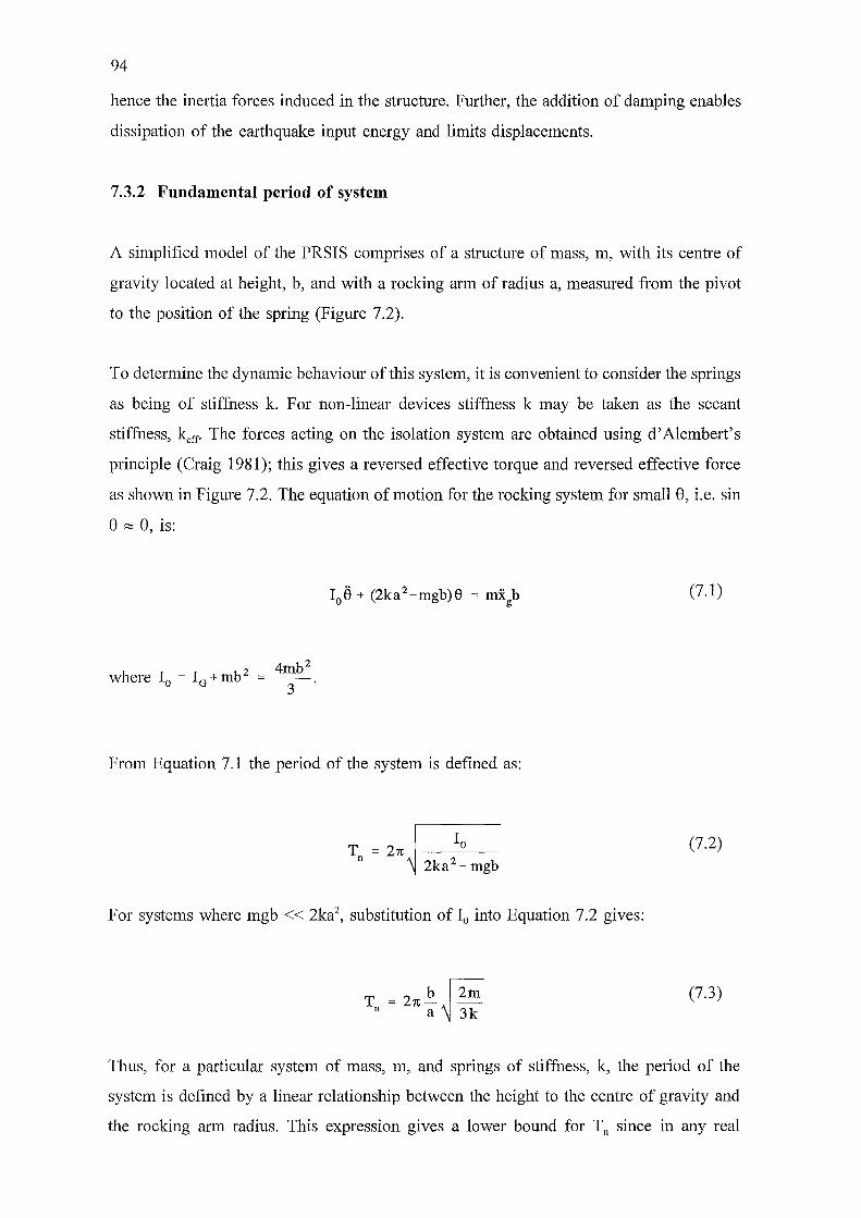
94
hence the inertia forces induced in the structure. Further, the addition of damping enables
dissipation of the earthquake input energy and limits displacements.
7.3.2 Fundamental period of system
A simplified model of the PRSIS comprises of a structure of mass, m, with its centre of
gravity located at height, b, and with a rocking arm of radius a, measured from the pivot
to the position of the spring (Figure 7.2).
To determine the dynamic behaviour of this system, it is convenient to consider the springs
as being of stiffness k. For non-linear devices stiffness k may be taken as the secant
stiffness, kerr· The forces acting on the isolation system are obtained using d' Alembert's
principle (Craig 1981); this gives a reversed effective torque and reversed effective force
as shown in Figure 7.2. The equation of motion for the rocking system for small 8, i.e. sin
8 r:::; 8, is:
(7.1)
where I = I + mb 2 0 G
4mb 2 ---
3
From Equation 7.1 the period of the system is defined as:
(7.2) 2ka 2 -mgb
For systems where mgb << 2lca2, substitution of 10 into Equation 7.2 gives:
T = 2n l ~ 2m n a 3k
(7.3)
Thus, for a particular system of mass, m, and springs of stiffness, k, the period of the
system is defined by a linear relationship between the height to the centre of gravity and
the rocking arm radius. This expression gives a lower bound for T n since in any real
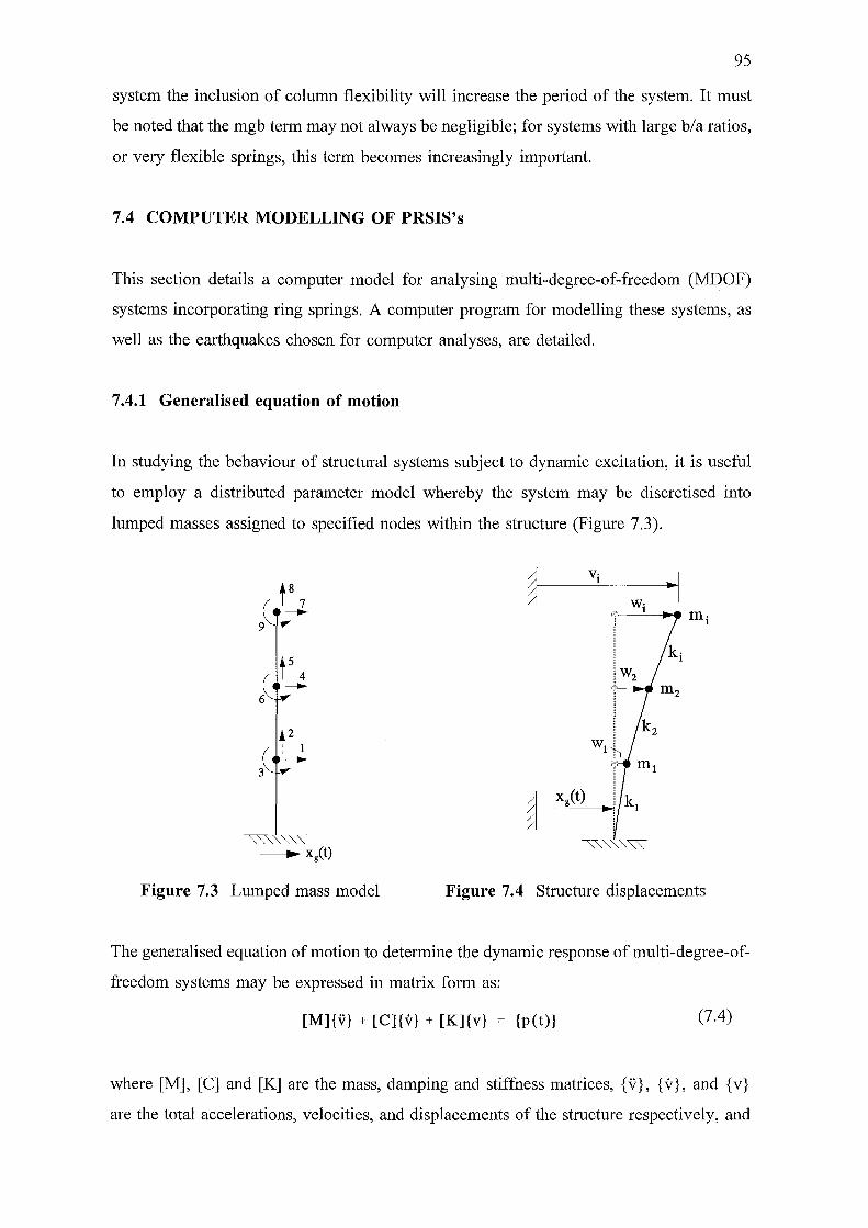
95
system the inclusion of column flexibility will increase the period of the system. It must
be noted that the mgb term may not always be negligible; for systems with large b/a ratios,
or very flexible springs, this term becomes increasingly important.
7.4 COMPUTER MODELLING OF PRSIS's
This section details a computer model for analysing multi-degree-of-freedom (MDOF)
systems incorporating ring springs. A computer program for modelling these systems, as
well as the earthquakes chosen for computer analyses, are detailed.
7.4.1 Generalised equation of motion
In studying the behaviour of structural systems subject to dynamic excitation, it is useful
to employ a distributed parameter model whereby the system may be discretised into
lumped masses assigned to specified nodes within the structure (Figure 7.3).
Figure 7.3 Lumped mass model Figure 7.4 Structure displacements
The generalised equation of motion to determine the dynamic response of multi-degree-of
freedom systems may be expressed in matrix form as:
[M]{v} + [C]{v} + [K]{v} = {p(t)} (7.4)
where [M], [C] and [K] are the mass, damping and stiffness matrices, {v}, {v}, and {v}
are the total accelerations, velocities, and displacements of the structure respectively, and
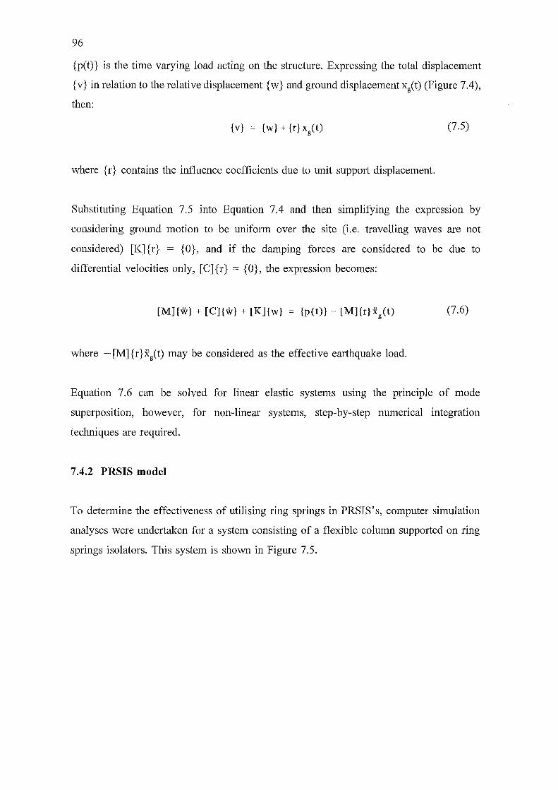
96
{p(t)} is the time varying load acting on the structure. Expressing the total displacement
{v} in relation to the relative displacement {w} and ground displacement xg(t) (Figure 7.4),
then:
{v} (7.5)
where {r} contains the influence coefficients due to unit support displacement.
Substituting Equation 7.5 into Equation 7.4 and then simplifying the expression by
considering ground motion to be uniform over the site (i.e. travelling waves are not
considered) [K] { r} = { 0}, and if the damping forces are considered to be due to
differential velocities only, [C]{r} = {0}, the expression becomes:
[M]{w} + [C]{w} + [K]{w} {p(t)}- [M]{r}xg(t) (7.6)
where -[M]{r}x-g(t) may be considered as the effective earthquake load.
Equation 7.6 can be solved for linear elastic systems using the principle of mode
superposition, however, for non-linear systems, step-by-step numerical integration
techniques are required.
7.4.2 PRSIS model
To determine the effectiveness of utilising ring springs in PRSIS's, computer simulation
analyses were undertaken for a system consisting of a flexible column supported on ring
springs isolators. This system is shown in Figure 7.5.
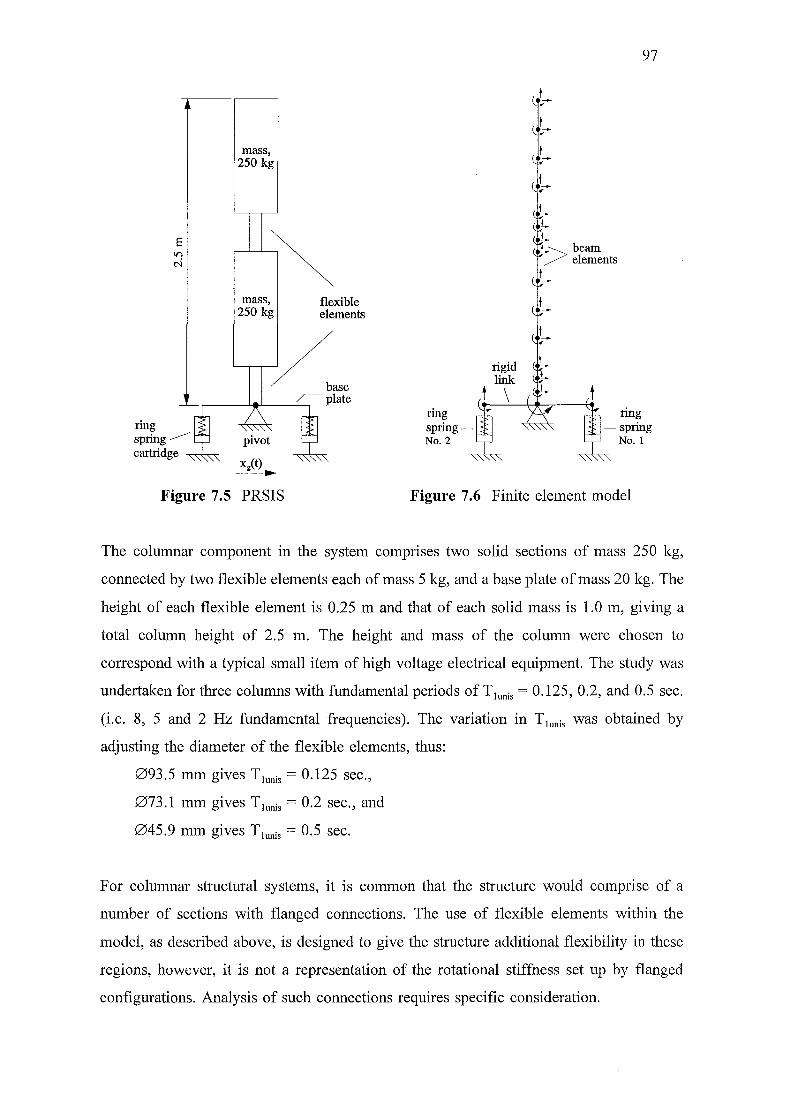
mass, 250 kg
mass, 250 kg
ring spring -----cartridge
Figure 7.5 PRSIS
flexible elements
ring springNo. 2
rigid link
\
97
!_
'-'-->beam / elements
L
ring -spring
No.1
Figure 7.6 Finite element model
The columnar component in the system comprises two solid sections of mass 250 kg,
connected by two flexible elements each of mass 5 kg, and a base plate of mass 20 kg. The
height of each flexible element is 0.25 m and that of each solid mass is 1.0 m, giving a
total column height of 2.5 m. The height and mass of the column were chosen to
correspond with a typical small item of high voltage electrical equipment. The study was
undertaken for three columns with fundamental periods of Ttunis = 0.125, 0.2, and 0.5 sec.
(i.e. 8, 5 and 2 Hz fundamental frequencies). The variation in T1unis was obtained by
adjusting the diameter of the flexible elements, thus:
093.5 mm gives T1unis = 0.125 sec.,
073.1 mm gives Ttunis = 0.2 sec., and
045.9 mm gives Ttunis = 0.5 sec.
For columnar structural systems, it is common that the structure would comprise of a
number of sections with flanged connections. The use of flexible elements within the
model, as described above, is designed to give the structure additional flexibility in these
regions, however, it is not a representation of the rotational stiffness set up by flanged
configurations. Analysis of such connections requires specific consideration.

98
The computer model of the isolation system is presented in Figure 7.6. The model
comprises beam elements with lumped nodal masses and rigid linlc elements modelling the
base plate. The ring spring elements represent bi-directional ring spring cartridges. These
elements are defined by the ring spring force/deflection characteristics. The stiffness values
chosen for the ring spring elements are as follows:
Ko = 2.5xl06 N/m
Ki = 385xl03 N/m
K 1 = 33xl06 N/m
Kd = 142x103 N/m
These values have been obtained from tests carried out on a prototype ring spring cartridge
reported in Section 4.5.2. Though these stiffness values apply to the ring spring chosen,
the same stiffnesses may be obtained for ring springs of different sizes simply by
increasing or decreasing the number of ring elements in a particular stack. The fundamental
period of the rocking system, T lis' based upon stiffness Ki for each of the three columns
is as follows: for the column of T1unis = 0.125 sec., the fundamental period of the isolated
system is Tlis = 1.006 sec; for the column of T1unis = 0.2 sec., the fundamental isolated
period is Tlis = 1.018 sec; and for the column of period T1unis = 0.5 sec., the fundamental
isolated period is T lis = 1.116 sec. These fundamental periods have been determined using
a computer program capable of modelling MDOF systems incorporating ring springs; this
program is now discussed.
7.4.3 RUAUMOKO computer program
The nng spnng model, as reported in section 5 .2.2, was incorporated within a
commercially available time history analysis software package - RUAUMOKO. This
program was initially written by Sharpe (1974), and has been significantly extended by
Carr (1995). RUAUMOKO uses the unconditionally stable Newmark constant average
acceleration (Newmark 13 = 0.25) method to compute the time history response of non
linear two-dimensional general frame structures subject to dynamic excitation. The ring
spring algorithm incorporated within RUAUMOKO is presented in Appendix A.
99
7.4.4 Earthquake excitations used in analyses
The PRSIS was subjected to six earthquakes: four short period and two long period. These
are detailed below.
(a) Short period type earthquakes
Short period type earthquakes are classed as those earthquakes whose dominant spectral
accelerations occur at periods less than about 0.8-1.0 second. Four such earthquakes were
chosen for the study. These are:
• El Centro 1940 N-S (Trifunac and Brune 1970)
• Pacoima Dam 1971 S16E (Oakeshott 1975)
• Parkfield 1966 N65E (Hausner and Trifunac 1967)
• El Centro 1979 N-S (Brandow and Leeds 1980)
Detailed discussion on the specific nature of these earthquakes may be found in the above
references; accelerograms of the earthquakes, as well as their response spectra, are
presented in Figures 7.7 and 7.8.
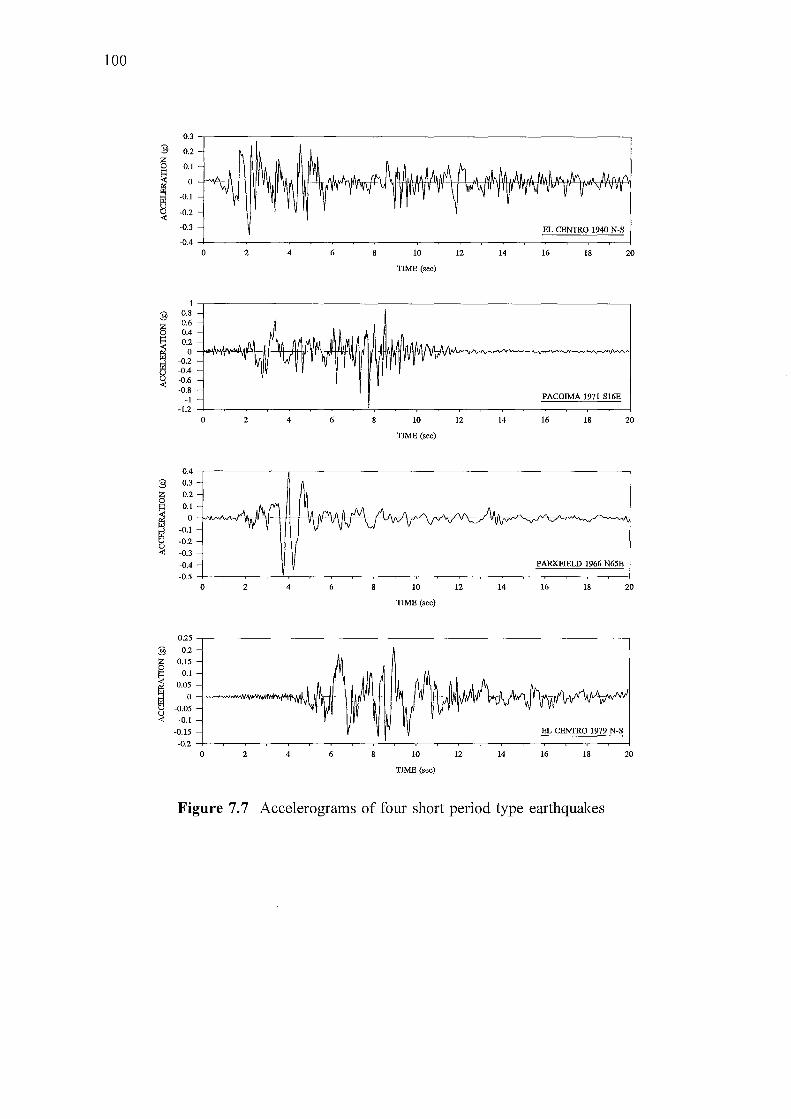
100
0.3,---------------------------------------------------------------.
3 0.2
~ 0.1
1:: -0.3 EL CENTRO 1940 N-S
-0.4 .L~_;_~~~~~~~-~~~~~-~~~~==:=~ 0 2 4 6 10
TIME (sec)
12 14 16 18 20
1 -,--------------------------------------------------------------, :§ 0.8 z 0.6 0 0.4
~~~ .::~ !:l -0.4
-0.6 -0.8
-1 PACOIMA 1971 S16E
-1.2 -+---~~--~----~--~~--'-~~--~----~--~~--~----~--~~--~
:§
0 2 4 6 10
TIME (sec)
12 14 16 18 20
0.4.------------.--------------------------------------------------, 0.3 0.2
0.1
0 ___,.,.,""""'-~'"-1'..-11-'\
-0.1
-0.2
-0.3
-0.4 PARKFIELD 1966 N65E
-0.5 -+-----~--~----'-.--~--~~--~~--~----~--~~--~----~--~~--~ 0 2 4 10
TIME (sec)
12 14 16 18 20
0.25 --.-----------------------------------------------------------------,
0.2
~ 0.15
~ 0.1 0:: 0.05
~ ~
-0.05
-0.1
-0.15 EL CENTRO 1979 N-S
-0.2 -+---~~--~----~--~~--~~--~--~~--~~--~--~~--~~--~ 0 2 4 6 10
TIME (sec)
12 14 16 18
Figure 7.7 Accelerograms of four short period type earthquakes
20
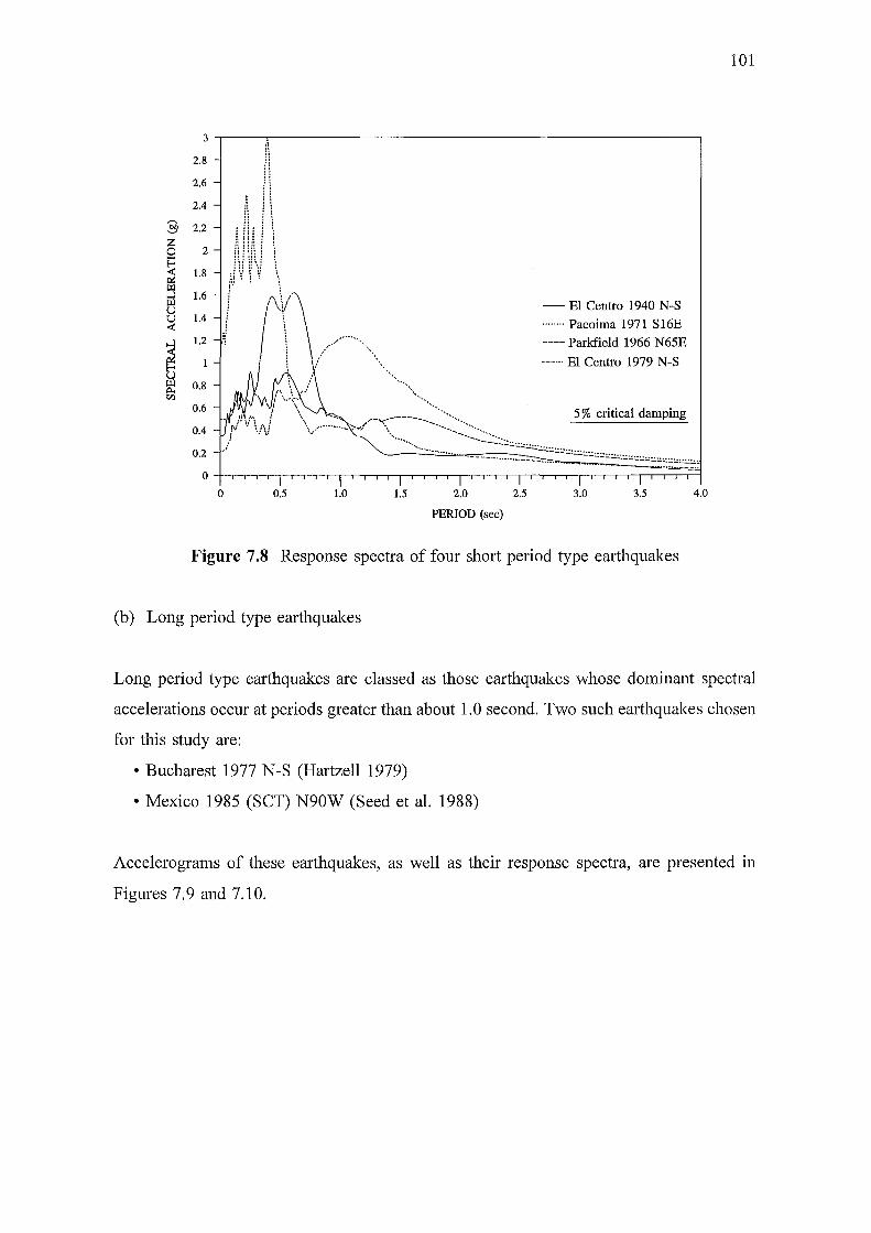
:§ z 0
~ ~ el u <:
~ Cl)
3
2.8
2.6
2.4
2.2
2
1.8
1.6
1.4
1.2
0.8
0.6
0.4
0.2
0
..
..... - ' ...... ... . . . ' Ill o I .. .
I 1\Y\ :! I \ I ·: I ~ \ •••• /······· •••
I i \/ ···.\. I ', :\ ·· .. I : :I "•,,,
!\ \ •. · \ ....... ; · .... ,~. \ '•
j \\ \ ······· .. .
- El Centro 1940 N-S ........ Pacoima 1971 S16E
----Parkfield 1966 N65E
.. ...... El Centro 1979 N-S
5% critical damping .Jt v \ i\ I '\ ... ~ ~ : ..... ~ ..... .~ ..... -";.~------ ........................ :·· ...
) ·: \J ·., -·-·-·-·---·-·---·-· --,~·~-~·.:::.:::::'-':.::.::.::.::::.::.::.::.::.::.::.::.::.::.::.::.::.::.::.::.::.::.::.::.::.::.::.::.::.::.::.:·
0 0.5 1.0 1.5 2.0
PERIOD (sec)
2.5 3.0 3.5 4.0
Figure 7.8 Response spectra of four short period type earthquakes
(b) Long period type earthquakes
101
Long period type earthquakes are classed as those earthquakes whose dominant spectral
accelerations occur at periods greater than about 1. 0 second. Two such earthquakes chosen
for this study are:
• Bucharest 1977 N-S (Hartzell 1979)
• Mexico 1985 (SCT) N90W (Seed et al. 1988)
Accelerograms of these earthquakes, as well as their response spectra, are presented in
Figures 7.9 and 7.10.
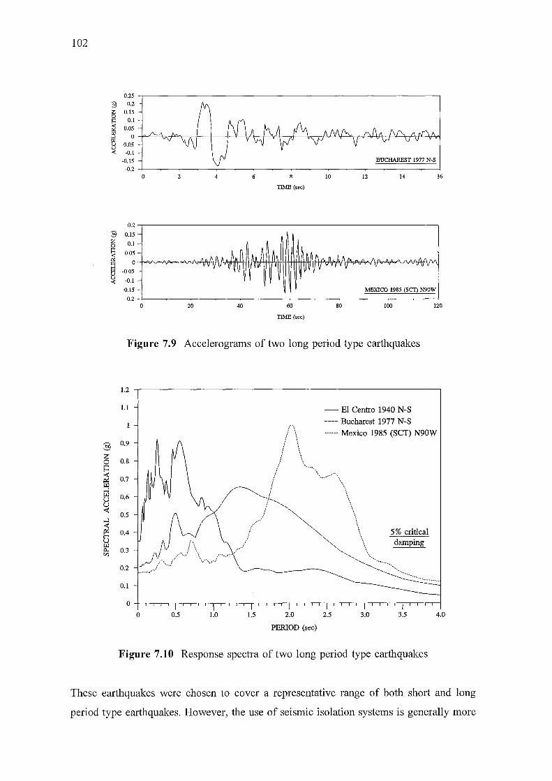
102
:§
I {.) {.)
<
:§ z 0
~ ~ {.) {.)
<
§ z 0 E=:
~ ~ el ~
~ te Cl)
0.25 0.2
0.15 0.1
0.05 0
-0.05 -0.1
-0.15 -0.2
0 2
0.2
0.15
0.1
0.05
0
-0.05
-0.1
-0.15
-0.2 0 20
4 6
40
TIME (sec)
60
TIME (sec)
10
80
BUCHAREST 1977 N-S
12 14 16
MEXICO 1985 (SCD N90W
100 120
Figure 7.9 Accelerograms of two long period type earthquakes
1.2 -r-------------------------------,
1.1
0.9
0.8
0.7
0.6
0.5
0.4
0.3
0.2
0.1
0
0 0.5 1.0 1.5 2.0
PERIOD (sec)
- El Centro 1940 N-S
---- Bucharest 1977 N-S
········ Mexico 1985 (SCT) N90W
2.5 3.0
5% critical damping
3.5 4.0
Figure 7.10 Response spectra of two long period type earthquakes
These earthquakes were chosen to cover a representative range of both short and long
period type earthquakes. However, the use of seismic isolation systems is generally more

103
suited to structures subjected to short period type earthquakes. This is because the addition
of flexibility moves the period of the system away from the vicinity of dominant spectral
accelerations. However, for structures exposed to long period type earthquakes, inclusion
of additional flexibility, could lead to a period shift into a region of increased spectral
accelerations. For these systems, an earthquake-resistant design that incorporates devices
that do not lengthen the period of the structure, but provide increased amounts of damping,
would be desirable. Such devices would include viscous dampers.
The likely characteristics of an earthquake at a particular site are important since this
determines which aseismic design method is appropriate. Several earthquakes recorded in
New Zealand recently, have shown response spectra characteristics similar to those of short
period type earthquakes (Sritharan and Dowrick 1994). These sites may be appropriate for
use of seismic isolation systems.
However, for completeness of the computer simulation analyses, both short and long period
type earthquakes are considered.
7.5 COMPUTER SIMULATION RESULTS FOR ISOLATED (PRSIS) AND
UNISOLATED SYSTEMS
This section details results of computer simulation analyses (using RUAUMOKO) for
isolated (PRSIS) and unisolated systems consisting of a column ofT1unis = 0.2 seconds and
subjected to the El Centro 1940 N-S earthquake. The following cases are analysed:
• unisolated (fixed base)
• PRSIS with 0% pre-displacement and 0% pre-load
• PRSIS with 16% pre-displacement and 0% pre-load
• PRSIS with 16% pre-displacement and 10% pre-load
• PRSIS with 16% pre-displacement and 20% pre-load
To compare the magnitude of loading experienced by each of these systems, the structure
bending moment for each case was determined. Bending moments were used as the
structure shear forces contribute only a few percent toward the total structural load.
The graphical results presented in the following sub-sections give the bending moment time
histories measured at the base of the structure; for all cases studied the maximum bending

104
moment occurred at this point.
The RUAUMOKO results for all cases considered were obtained using a consistent mass
matrix, constant damping of 2% applied to all modes, and a time step of 0.0001 sec. This
time step was shown to give a converged solution for the analyses considered. Also, 2%
damping was chosen to be representative of lightly damped systems. A small displacement
analysis was used and to avoid the high frequencies of the structure in the y direction, the
y degrees of freedom of the column were constrained.
The results of the computational analyses are presented graphically in Sections 7. 5.1, 7. 5 .2,
and 7.5.3. These are then discussed in Section 7.5.4.

105
7.5.1 Dynamic response of unisolated systems
The unisolated system was modelled by constraining the x, y and 8 degrees-of-freedom at
the base of the column (Figure 7.6). The bending moment time history for the unisolated
system subjected to the El Centro 1940 N-S earthquake is presented in Figure 7 .11.
s 6
~ 4
; 2
~ 0
I -2
-4 Unlsolated
-6 0 2 4 6 8 10 12 14 16 18 20 22 24
TIME (sec)
Figure 7.11 Dynamic response of unisolated system: bending moment time history
7.5.2 Dynamic response of pre-displaced PRSIS's
(a) 0% pre-displacement
The graphical results presented for the 0% pre-displaced 0% pre-loaded PRSIS subjected
to the El Centro 1940 N-S earthquake are:
• bending moment time history - measured at the base node (Figure 7.12 (a))
• ring spring cartridge displacement for spring No. 1 (Figure 7.12 (b))
• force/deflection response curve for spring No. 1 (Figure 7.12 (c))
Ring spring cartridge No. 1 is shown in Figure 7.6.
(b) 16% pre-displacement
The graphical results presented for the 16% pre-displaced 0% pre-loaded PRSIS subjected
to the El Centro 1940 N-S earthquake are:
• bending moment time history- measured at the base node (Figure 7.13 (a))
• ring spring cartridge displacement for spring No. 1 (Figure 7.13 (b))
• force/deflection response curve for spring No. 1 (Figure 7.13 (c))
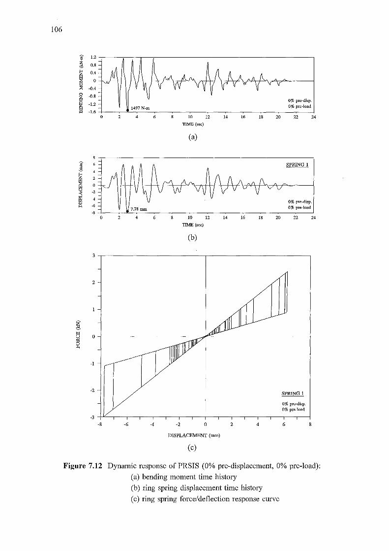
106
a 1.2
~ 0.8
i 0.4
0
~ -0.4
~ -0.8
ffi -1.2
1497 N-m ill -1.6
0 2 4 6
I 6
4
i 2
0 t:l -2
~ -4 s -6
-8 0 2 4 6
3
2
0
-1
-2
-8 -6 -4
8 10 12 14
TIME (sec)
(a)
8 10 12 14
TIME (sec)
(b)
-2 0 2
DISPLACEMENT (nun)
(c)
16 18 20
16 18 20
4
0% pre-disp. 0% pre-load
22 24
SPRING 1
0% pre-disp. 0% pre-load
22 24
SPRING 1
0% pre-disp. 0% pre-load
6 8
Figure 7.12 Dynamic response of PRSIS (0% pre-displacement, 0% pre-load):
(a) bending moment time history
(b) ring spring displacement time history
(c) ring spring force/deflection response curve
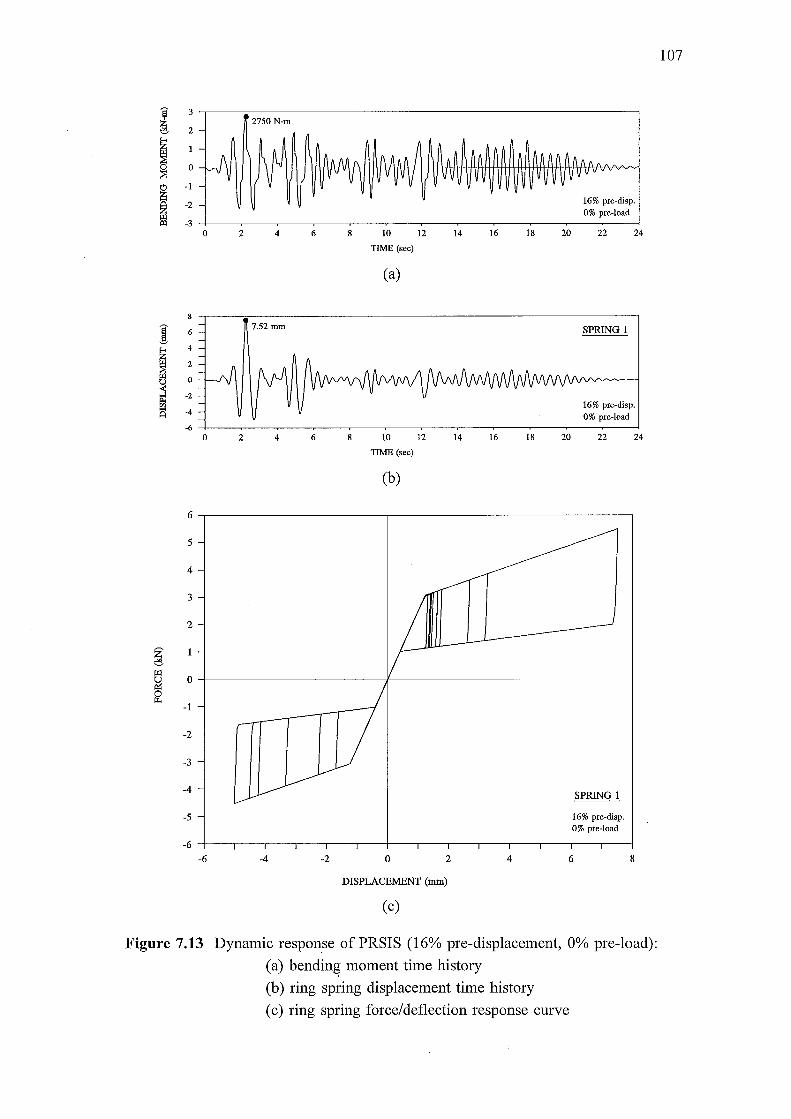
3 .-----~-------------------------------------------------. 2750 N-m
2
o~~~~H4~~~~~~~~~~~
-1
-2 16% pre-disp. 0% pre-load
-3 ~--~----~--~--~----~--~--~----~--~----~--~--~
4
2
0 2 4
7.52 mm
6 8 10
TIME (sec)
(a)
0 ---t-..J-"'f+t-+-i~"'-t-tt-i'-fficf\/"P'\Atttti-V'-tN-'r-1
-2
-4
12 14 16 18 20 22 24
SPRING 1
16% pre-disp. 0% pre-load
-6 ~--~----~--~--~----~--~--~----~--~----~--~--~ 0 2 4 6 10 12 14 16 18 20 22
TIME (sec)
(b)
6,-----------------------,-------------------------------,
5
4
3
2
0 ,_ _______________________ ,________________ --------------1
-1
-2
-3
-4
-5 16% pre-disp. 0% pre-load
-6 ~------.---.---.---.---~------.---.---.---.---.---.---~
24
-6 -4 -2 0 2 4 6 8
DISPLACEMENT (mm)
(c)
Figure 7.13 Dynamic response of PRSIS (16% pre-displacement, 0% pre-load):
(a) bending moment time history
(b) ring spring displacement time history
(c) ring spring force/deflection response curve
107
108
7.5.3 Dynamic response of pre:..displaced pre-loaded PRSIS's
(a) 16% pre-displacement 10% pre-load
The graphical results presented for the 16% pre-displaced 10% pre-loaded PRSIS subjected
to the El Centro 1940 N-S earthquake are:
• bending moment time history- measured at the base node (Figure 7.14 (a))
• ring spring cartridge displacement for spring No. 1 (Figure 7.14 (b))
• ring spring cartridge displacement for spring No. 2 (Figure 7.14 (c))
• force/deflection response curve for spring No. 1 (Figure 7.15 (a))
• force/deflection response curve for spring No. 2 (Figure 7.15 (b))
Ring spring cartridges No. 1 and 2 are shown in Figure 7.6.
(b) 16% pre-displacement 20% pre-load
The graphical results presented for the 16% pre-displaced 20% pre-loaded PRSIS subjected
to the El Centro 1940 N-S earthquake are:
• bending moment time history -measured at the base node (Figure 7.16 (a))
• ring spring cartridge displacement for spring No. 1 (Figure 7.16 (b))
• ring spring cartridge displacement for spring No. 2 (Figure 7.16 (c))
• force/deflection response curve for spring No. 1 (Figure 7.17 (a))
• force/deflection response curve for spring No.2 (Figure 7.17 (b))
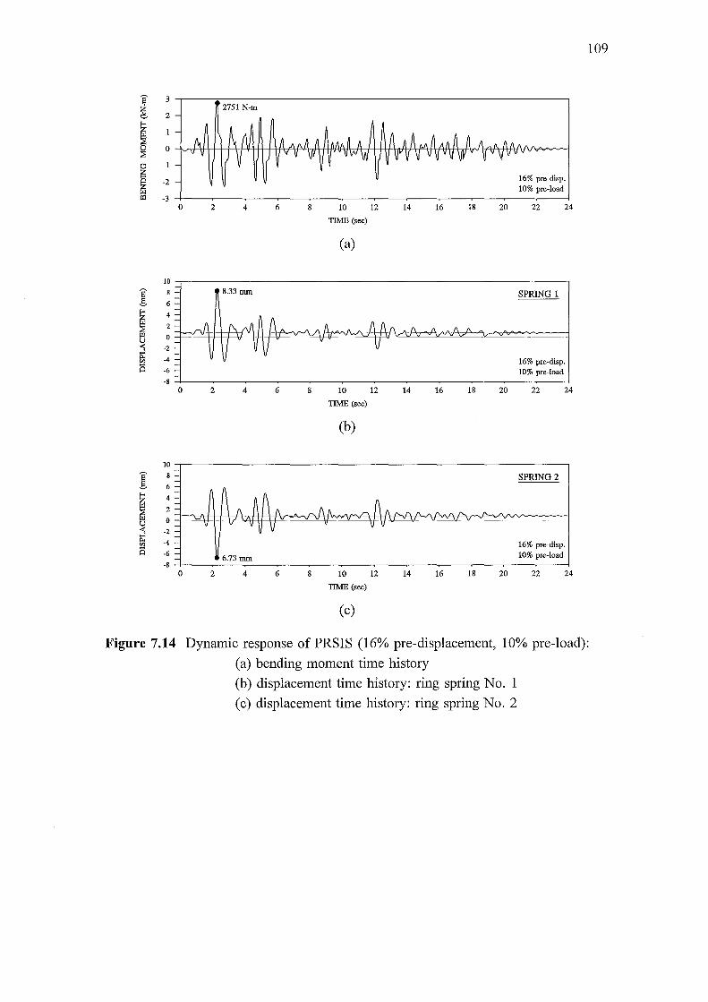
109
~ 3
g 2751 N-m 2
; ~ 0
I -1
-2 16% pre-disp. 10% pre-load
-3 0 2 4 6 10 12 14 16 18 20 22 24
TIME (sec)
(a)
10
I 8 SPRING 1 6
; 4
2
f:l 0
~ -2
-4 16% pre-disp. s -6 10% pre-load -8
0 2 4 6 8 10 12 14 16 18 20 22 24
TIME (sec)
(b)
10
I SPRING 2
~ 4
2
u 0
~ -2
~ -4 16% pre-disp. -6 10% pre-load -8
0 2 4 6 8 10 12 14 16 18 20 22 24
TIME (sec)
(c)
Figure 7.14 Dynamic response of PRSIS (16% pre-displacement, 10% pre-load):
(a) bending moment time history
(b) displacement time history: ring spring No. 1
(c) displacement time history: ring spring No. 2
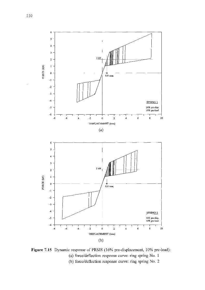
110
6 .----------------------,----------------------------.
5
4
3
2
0
-1
-2
-3
-4
-5
-8 -6 -4 -2 0 2 4
DISPLACEMENT (mm)
(a)
6
SPRING 1
16% pre-disp. 10% pre-load
8 10
6 .----------------------,----------------------------.
5
4
3
2
0
-1
-2
-3
-4
-5
-8 -6 -4 -2 0 2 4
DISPLACEMENT (mm)
(b)
6
SPRING2
16% pre-disp. 10% pre-load
8 10
Figure 7.15 Dynamic response of PRSIS (16% pre-displacement, 10% pre-load):
(a) force/deflection response curve: ring spring No. 1
(b) force/deflection response curve: ring spring No. 2
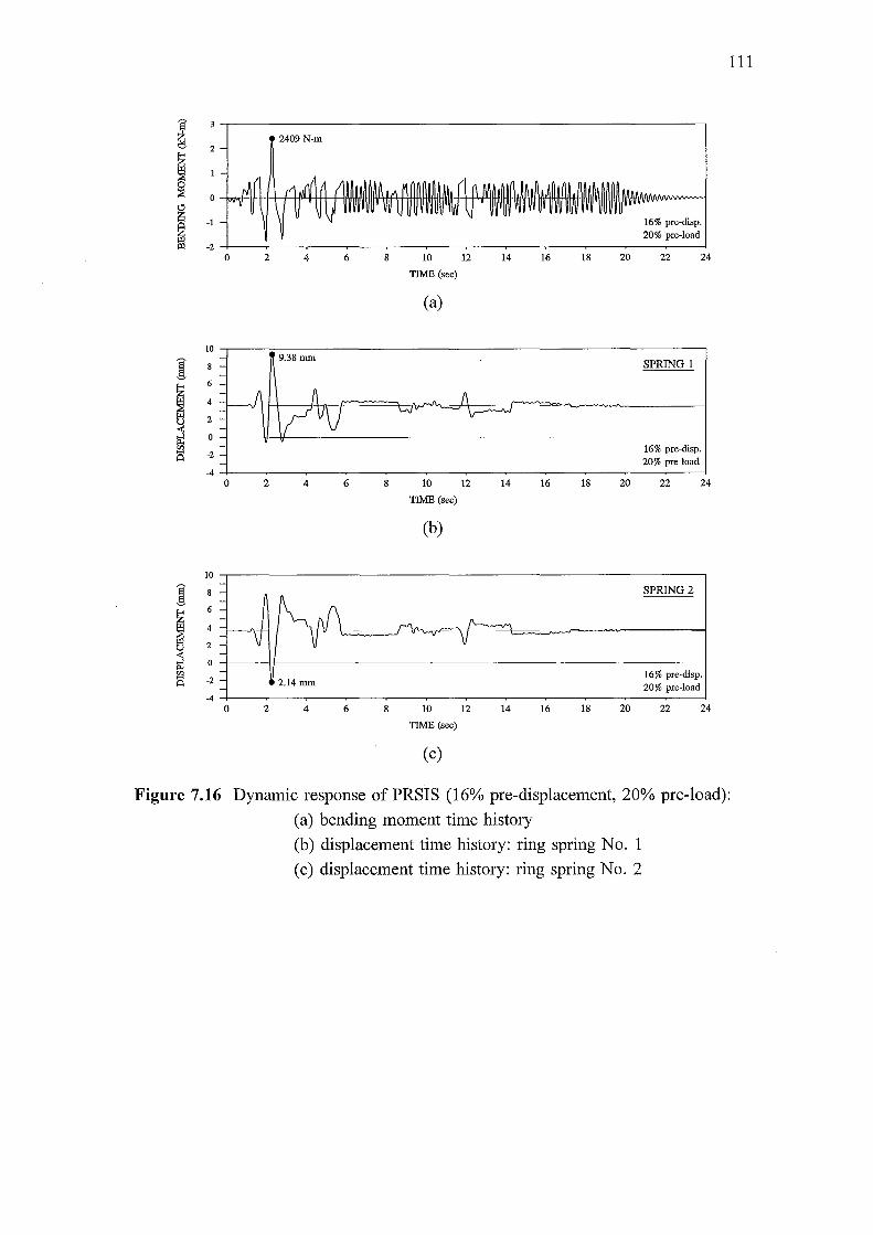
111
i ~ 2409 N-m
2 ; ~ 0
i -1 16% pre-disp. 20% pre-load
-2 0 2 4 6 8 10 12 14 16 18 20 22 24
TIME (sec)
(a)
10
I SPRING 1
~ 6
4
2
~ 0
iS -2 16% pre-disp. 20% pre-load
-4 0 2 4 6 10 12 14 16 18 20 22 24
TIME (sec)
(b)
10
I SPRING2
I 6
4
2
0 (/) 16% pre-disp. S -2
20% pre-load -4
0 2 4 6 8 10 12 14 16 18 20 22 24
TIME (sec)
(c)
Figure 7.16 Dynamic response of PRSIS (16% pre-displacement, 20% pre-load):
(a) bending moment time history
(b) displacement time history: ring spring No. 1
(c) displacement time history: ring spring No. 2
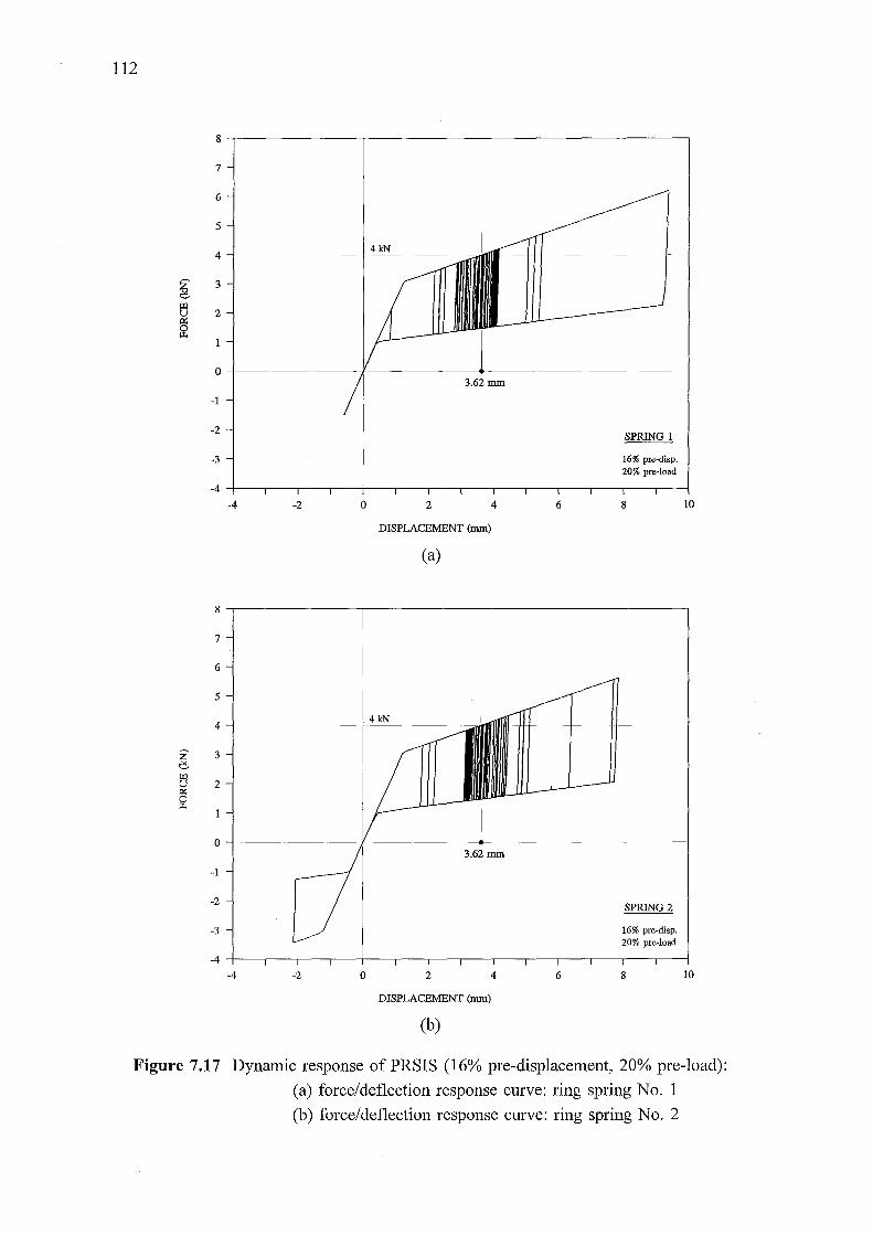
112
8.--------------,------------------------------------,
7
6
5
4
3
2
0
-1
-2
-3
-4 -2 0 2 4 6
DISPLACEMENT (mm)
(a)
SPRING 1
16% pre-disp. 20% pre-load
8 10
8 .--------------,------------------------------------,
7
6
5
4
3
2
0
-1
-2
-3
SPRING2
16% pre-disp. 20% pre-load
-4 1---.---~-.---+--~--~--.---.---.--.---.---r--.-~
-4 -2 0 2 4 6 8 10
DISPLACEMENT (mm)
(b)
Figure 7.17 Dynamic response of PRSIS (16% pre-displacement, 20% pre-load):
(a) force/deflection response curve: ring spring No. 1
(b) force/deflection response curve: ring spring No. 2
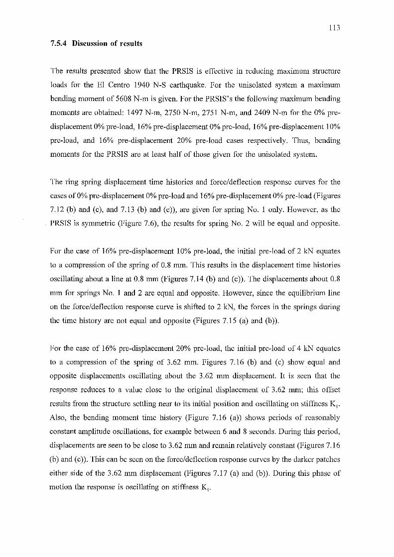
113
7.5.4 Discussion of results
The results presented show that the PRSIS is effective in reducing maximum structure
loads for the El Centro 1940 N-S earthquake. For the unisolated system a maximum
bending moment of 5608 N-m is given. For the PRSIS's the following maximum bending
moments are obtained: 1497 N-m, 2750 N-m, 2751 N-m, and 2409 N-m for the 0% pre
displacement 0% pre-load, 16% pre-displacement 0% pre-load, 16% pre-displacement 10%
pre-load, and 16% pre-displacement 20% pre-load cases respectively. Thus, bending
moments for the PRSIS are at least half of those given for the unisolated system.
The ring spring displacement time histories and force/deflection response curves for the
cases ofO% pre-displacement 0% pre-load and 16% pre-displacement 0% pre-load (Figures
7.12 (b) and (c), and 7.13 (b) and (c)), are given for spring No.1 only. However, as the
PRSIS is symmetric (Figure 7.6), the results for spring No. 2 will be equal and opposite.
For the case of 16% pre-displacement 10% pre-load, the initial pre-load of 2 kN equates
to a compression of the spring of 0.8 mm. This results in the displacement time histories
oscillating about a line at 0.8 mm (Figures 7.14 (b) and (c)). The displacements about 0.8
mm for springs No. 1 and 2 are equal and opposite. However, since the equilibrium line
on the force/deflection response curve is shifted to 2 kN, the forces in the springs during
the time history are not equal and opposite (Figures 7.15 (a) and (b)).
For the case of 16% pre-displacement 20% pre-load, the initial pre-load of 4 kN equates
to a compression of the spring of 3. 62 mm. Figures 7.16 (b) and (c) show equal and
opposite displacements oscillating about the 3.62 mm displacement. It is seen that the
response reduces to a value close to the original displacement of 3.62 mm; this offset
results from the structure settling near to its initial position and oscillating on stiffness K1•
Also, the bending moment time history (Figure 7.16 (a)) shows periods of reasonably
constant amplitude oscillations, for example between 6 and 8 seconds. During this period,
displacements are seen to be close to 3. 62 mm and remain relatively constant (Figures 7.16
(b) and (c)). This can be seen on the force/deflection response curves by the darker patches
either side ofthe 3.62 mm displacement (Figures 7.17 (a) and (b)). During this phase of
motion the response is oscillating on stiffness K1•
114
7.6 MAXIMUM STRUCTURE BENDING MOMENTS FOR ISOLATED AND
UNISOLATED SYSTEMS
The above analyses have been repeated to consider a comprehensive range of isolated
(PRSIS) and unisolated systems subjected to the six different earthquake excitations.
The systems analysed were for the flexible column with unisolated fundamental periods
of:
Tiunis = 0.125 seconds
T 1unis = 0.2 seconds
T I unis = 0. 5 seconds
and used in the following system configurations:
• unisolated (fixed base)
• PRSIS with 0% pre-displacement and 0% pre-load
• PRSIS with 16% pre-displacement and 0% pre-load
• PRSIS with 16% pre-displacement and 10% pre-load
• PRSIS with 16% pre-displacement and 20% pre-load
Tabular results for all cases studied are presented in Appendix C. These tables give the
maximum structure bending moment for the isolated and unisolated systems for each
earthquake input. The case for T1unis = 0.2 seconds, and for 0% pre-displacement 0% pre
load, is presented in Table 7.1.
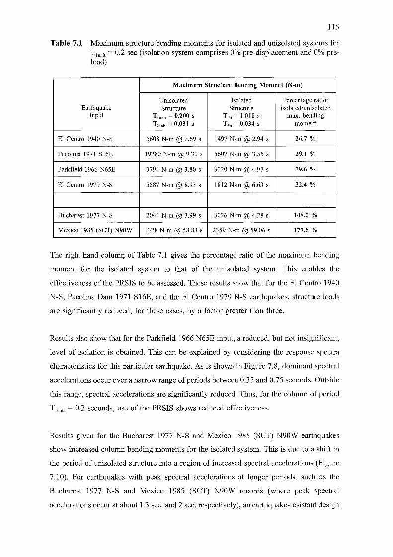
115
Table 7.1 Maximum structure bending moments for isolated and unisolated systems for T1unis = 0.2 sec (isolation system comprises 0% pre-displacement and 0% preload)
Maximum Structure Bending Moment (N-m)
Unisolated Isolated Percentage ratio: Earthquake Structure Structure isolated/unisolated
Input Tlunis = 0.200 S Tlis = 1.018 S max. bending Tzunis = 0.031 S T2;, = 0.034 S moment
El Centro 1940 N-S 5608 N-m @ 2.69 s 1497 N-m@ 2.94 s 26.7%
Pacoima 1971 S16E 19280 N-m @ 9.31 s 5607 N-m @ 3.55 s 29.1%
Parkfield 1966 N65E 3794 N-m@ 3.80 s 3020 N-m @ 4.97 s 79.6%
El Centro 1979 N-S 5587 N-m @ 8.93 s 1812 N-m@ 6.63 s 32.4%
Bucharest 1977 N-S 2044 N-m @ 3.99 s 3026 N-m @ 4.28 s 148.0%
Mexico 1985 (SCT) N90W 1328 N-m @ 58.83 s 2359 N-m @ 59.06 s 177.6%
The right hand column of Table 7.1 gives the percentage ratio of the maximum bending
moment for the isolated system to that of the unisolated system. This enables the
effectiveness of the PRSIS to be assessed. These results show that for the El Centro 1940
N-S, Pacoima Dam 1971 S16E, and the El Centro 1979 N-S earthquakes, structure loads
are significantly reduced; for these cases, by a factor greater than three.
Results also show that for the Parkfield 1966 N65E input, a reduced, but not insignificant,
level of isolation is obtained. This can be explained by considering the response spectra
characteristics for this particular earthquake. As is shown in Figure 7.8, dominant spectral
accelerations occur over a narrow range of periods between 0. 3 5 and 0. 7 5 seconds. Outside
this range, spectral accelerations are significantly reduced. Thus, for the column of period
T1unis = 0.2 seconds, use of the PRSIS shows reduced effectiveness.
Results given for the Bucharest 1977 N-S and Mexico 1985 (SCT) N90W earthquakes
show increased column bending moments for the isolated system. This is due to a shift in
the period of unisolated structure into a region of increased spectral accelerations (Figure
7.1 0). For earthquakes with peak spectral accelerations at longer periods, such as the
Bucharest 1977 N-S and Mexico 1985 (SCT) N90W records (where peak spectral
accelerations occur at about 1.3 sec. and 2 sec. respectively), an earthquake-resistant design
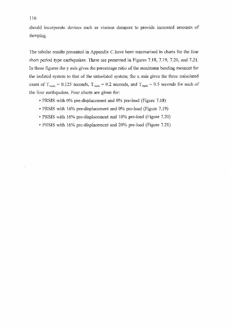
116
should incorporate devices such as viscous dampers to provide increased amounts of
damping.
The tabular results presented in Appendix C have been summarised in charts for the four
short period type earthquakes. These are presented in Figures 7.18, 7.19, 7.20, and 7.21.
In these figures the y axis gives the percentage ratio of the maximum bending moment for
the isolated system to that of the unisolated system; the x axis gives the three unisolated
cases of T1unis = 0.125 seconds, T1unis = 0.2 seconds, and T1unis = 0.5 seconds for each of
the four earthquakes. Four charts are given for:
• PRSIS with 0% pre-displacement and 0% pre-load (Figure 7.18)
• PRSIS with 16% pre-displacement and 0% pre-load (Figure 7.19)
• PRSIS with 16% pre-displacement and 10% pre-load (Figure 7.20)
• PRSIS with 16% pre-displacement and 20% pre-load (Figure 7.21)
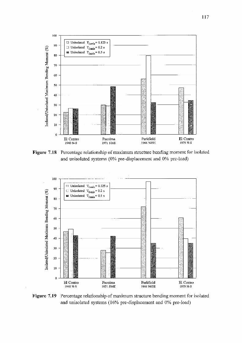
100 ,---------------------------------------------------------,
90 0 Unisolated Tlunis= 0.125 s
~--------------~-------------
0 Unisolated T1unis= 0.2 s
80 1111 Unisolated T1unis = 0.5 s
70 4----------------~------------------~
40 1---------------------
20
10
El Centro 1940 N-S
Pacoima 1971 S16E
Parkfield 1966 N65E
El Centro 1979 N-S
117
Figure 7.18 Percentage relationship of maximum structure bending moment for isolated
and unisolated systems (0% pre-displacement and 0% pre-load)
100 .---------------------------------------------------------.
90 D Unisolated T1unis= 0.125 s
1-----------------1 D Unisolated Tlunis = 0.2 s
80 1111 Unisolated Tlunis = 0.5 s
60 4---------------------~----
40
30
20
10
El Centro 1940 N-S
Pacoima 1971 S16E
Parkfield 1966 N65E
El Centro 1979 N-S
Figure 7.19 Percentage relationship of maximum structure bending moment for isolated
and unisolated systems (16% pre-displacement and 0% pre-load)
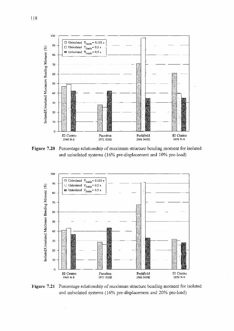
118
100 ~--------------------------------------------------------.
90
80
D Unisolated Tlunis~ 0.125 s 1----·----------1
D Unisolated T1unis~ 0.2 s
IIIII Unisolated T1unis ~ 0.5 s
El Centro 1940 N-S
Pacoima 1971 S16E
Parkfield 1966 N65E
El Centro 1979 N-S
Figure 7.20 Percentage relationship of maximum structure bending moment for isolated
and unisolated systems (16% pre-displacement and 10% pre-load)
100 .---------------------------------------------------------.
90
80
40
30
20
10
D Unisolated T1unis~ 0.125 s ~--------~-.--------------~
D Unisolated Tlunis~ 0.2 s
El Centro 1940 N-S
Pacoima 1971 S16E
Parkfield 1966 N65E
El Centro 1979 N-S
Figure 7.21 Percentage relationship of maximum structure bending moment for isolated
and unisolated systems (16% pre-displacement and 20% pre-load)
119
7.6.1 Discussion of summarised results
The results show that structural loads experienced during short period type earthquakes,
can be significantly reduced utilising pivotal rocking seismic isolation systems. Structure
bending moments were reduced by factors of approximately 2-3 or greater in some cases.
The exceptions were the isolation systems incorporating flexible columns of period T1unis
= 0.125 and 0.2 seconds, subjected to the Parkfield 1966 N65E earthquake.
Results were obtained for an isolation system fundamental period (Tlis) of approximately
1. 0- 1.1 seconds, suggesting that these periods are sufficient to ensure effective isolation.
The maximum rotation of the isolation system base plate occurred for the system of period
Tlis = 1.116 sec (0% pre-displacement and 0% pre-load) when subjected to the Pacoima
Dam 1971 S16E earthquake. A maximum base rotation of 7.8° was obtained.
Generally, ring spring pre-displacement and pre-load did not have a significant effect on
the results. However, in practical systems it would be desirable to keep both the pre
displacement and pre-load small, thus allow a larger displacement range for a given ring
spring cartridge.
In addition to the computer simulation results presented, the effect of using a large
displacement analysis was studied. This enabled changes in the geometry of the system,
as well as gravity effects of the column self weight, to be considered. Two pre-displaced
pre-loaded systems subjected to the El Centro 1940 N-S earthquake were analysed. Results
for these systems are as follows:
• 16% pre-displacement 0% pre-load (T1unis = 0.2 sec):
bending moment (max.) = 2708 N-m @ 2.23 sec (large displacement analysis)
bending moment (max.) = 2750 N-m @ 2.24 sec (small displacement analysis)
• 16% pre-displacement 20% pre-load (T1unis = 0.2 sec):
bending moment (max.) = 2419 N-m @ 2.24 sec (large displacement analysis)
bending moment (max.) = 2409 N-m @ 2.25 sec (small displacement analysis)
These results show differences of less than 2% for large and small displacement analyses.
120
Further, the influence of simultaneously applying both the horizontal and vertical
components of an earthquake to a PRSIS was studied. For PRSIS's, vertical inputs are fed
directly through the pivot into the column. Hence to determine the effect on structure
bending moment, two pre-displaced pre-loaded systems, subjected to the El Centro 1940
N-S and El Centro 1940 U-D (ve1iical) earthquakes simultaneously, were analysed. Results
for these systems are as follows:
• 16% pre-displacement 0% pre-load (T1unis = 0.2 sec):
bending moment (max.) = 2708 N-m @ 2.23 sec (large displacement analysis)
• 16% pre-displacement 20% pre-load (T1unis = 0.2 sec):
bending moment (max.) = 2420 N-m@ 2.24 sec (large displacement analysis)
These results are almost identical to those above for the El Centro 1940 N-S earthquake
only. However, the effect on column bending moment would be more noticeable in cases
where a structure is deformed near to its maximum and is then subject to a large vertical
input.
7.7 SUMMARY
Ring springs have been identified as possible candidates for use in rocking/stepping seismic
isolation systems. The potential benefits of utilising ring springs in these applications have
been outlined.
Subsequently, a pivotal rocking seismic isolation system (PRSIS) incorporating ring springs
was developed. To determine the effectiveness of utilising ring springs in these systems,
computer simulation analyses were undertaken. The study investigated the behaviour of
isolated and unisolated systems subject to six different earthquake inputs.
Results show that for columnar structures with fundamental periods between 0.125-0.5
seconds, PRSIS' s can significantly reduce structural loads during short period type
earthquakes. To confirm the performance of these isolation systems, experimental testing
of a PRSIS subjected to a range of earthquake excitations, is required.
Chapter 8
DEVELOPMENT OF A PROTOTYPE PIVOTAL ROCKING
SEISMIC ISOLATION SYSTEM: EXPERIMENTAL
TESTING AND COMPUTER SIMULATION
8.1 INTRODUCTION
121
Results of computer simulation analyses, as reported in Chapter 7, show that pivotal
rocking seismic isolation systems can significantly reduce structural loads during short
period type earthquakes. This chapter details the design and testing of a manufactured
PRSIS. Initially, design details of the PRSIS are presented, followed by results of shaker
table tests. These test results, for both isolated and unisolated systems, are then compared
with results given by computer simulation.
8.2 DESIGN OF A PROTOTYPE PIVOTAL ROCKING SEISMIC ISOLATION SYSTEM
This section details the design of a prototype PRSIS consisting of a pivot mechanism and
a series of ring spring cartridge assemblies.
8.2.1 Pivot mechanism
A Hooke's joint was chosen for the PRSIS pivot mechanism. This selection was made
primarily because of the simplicity and ease of manufacture of a Hooke's joint.
8.2.2 Uni-directional ring spring cartridges
In conjunction with the pivot mechanism, a system of four ring spring assemblies fitted at
90° intervals around the periphery of a stiff base, was developed. Symmetry of this design
enables the system to be analysed as an equivalent two-dimensional system for inputs
applied in line, as well as at an angle of 45°, with the axes of the ring spring cartridges.
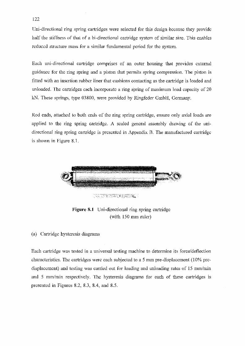
122
Uni-directional ring spring cartridges were selected for this design because they provide
half the stiffness of that of a bi-directional cartridge system of similar size. This enables
reduced structure mass for a similar fundamental period for the system.
Each uni-directional cartridge comprises of an outer housing that provides external
guidance for the ring spring and a piston that permits spring compression. The piston is
fitted with an insertion rubber liner that cushions contacting as the cartridge is loaded and
unloaded. The cartridges each incorporate a ring spring of maximum load capacity of 20
kN. These springs, type 03800, were provided by Ringfeder GmbH, Germany.
Rod ends, attached to both ends of the ring spring cartridge, ensure only axial loads are
applied to the ring spring cartridge. A scaled general assembly drawing of the uni
directional ring spring cartridge is presented in Appendix B. The manufactured cartridge
is shown in Figure 8.1.
Figure 8.1 Uni-directional ring spring cartridge
(with 150 mm ruler)
(a) Cartridge hysteresis diagrams
Each cartridge was tested in a universal testing machine to determine its force/deflection
characteristics. The cartridges were each subjected to a 5 mm pre-displacement (10% pre
displacement) and testing was carried out for loading and unloading rates of 15 mm/min
and 5 mm/min respectively. The hysteresis diagrams for each of these cartridges is
presented in Figures 8.2, 8.3, 8.4, and 8.5.
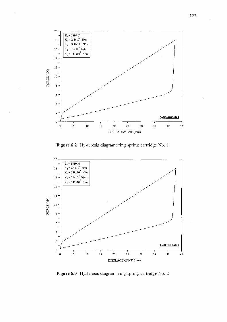
~ ~ ~ 0 ~
~ ~ 0 ~
20
18
16
14
12
10
8
6
4
2
0
0
F0 = 1890 N
K 0 = 2.4x10⁶ N/m 3
K 1 = 380x10 N/m
K 1 = 10x106
N/m 3
Kd = 141x10 N/m
5 10
CARTRIDGE 1
15 20 25 30 35 40
DISPLACEMENT (mm)
Figure 8.2 Hysteresis diagram: ring spring cartridge No. 1
20
18
16
14
12
10
8
6
4
2
0
0
F0 = 1810 N
K 0 = 2.4x10⁶ N/m 3
K 1 = 388x10 N/m
K 1 = llx106
N/m 3
Kd = 141x10 N/m
5 10
CARTRIDGE2
15 20 25 30 35 40
DISPLACEMENT (mm)
Figure 8.3 Hysteresis diagram: ring spring cartridge No. 2
123
45
45
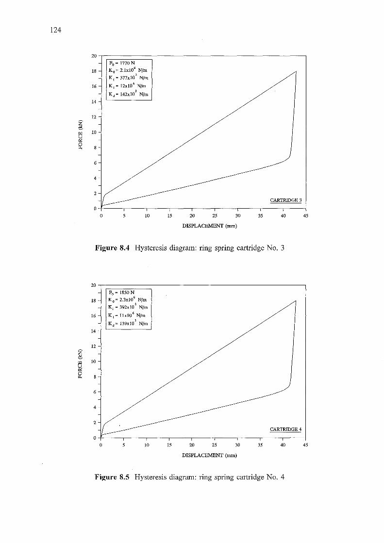
124
~ ~ ~ 0 JJ..
~
i
20
18
16
14
12
10
8
6
4
2
0
0
F0 =1770N
K 0 = 2.1x10⁶
N/m 3
K 1 = 377x10 N/m
K 1 = 12x106
N/m 3
Kd = 142x10 N/m
5 10
CARTRIDGE 3
15 20 25 30 35 40
DISPLACEMENT (mm)
Figure 8.4 Hysteresis diagram: ring spring cartridge No. 3
20
18
16
14
12
10
8
6
4
2
0
0
F0 = 1850 N
K 0 = 2.3x10⁶
N/m 3
K 1 = 392x10 Nfm
K 1 = llx106
N/m 3
Kd = 139x10 N/m
5 10
CARTRIDGE4
15 20 25 30 35 40
DISPLACEMENT (mm)
Figure 8.5 Hysteresis diagram: ring spring cartridge No. 4
45
45
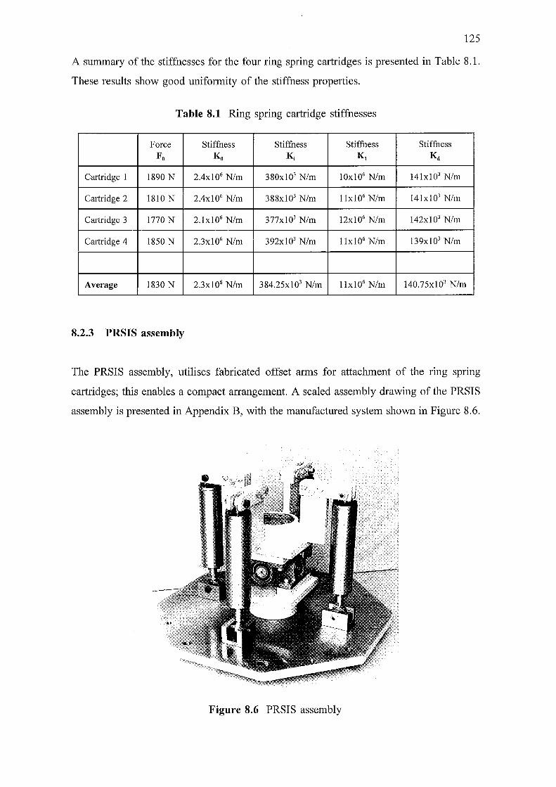
125
A summary of the stiffnesses for the four ring spring cartridges is presented in Table 8.1.
These results show good uniformity of the stiffness properties.
Table 8.1 Ring spring cartridge stiffnesses
Force Stiffness Stiffness Stiffness Stiffness Fo Ko K; Kt Kd
Cartridge 1 1890 N 2.4x10⁶ N/m 380xl03 N/m 10xl06 N/m 141x103 N/m
Cartridge 2 1810 N 2.4xl06 N/m 388xl03 N/m llxl06 N/m 141xl03 N/m
Cartridge 3 1770 N 2.1xl06 N/m 377x103 N/m 12xl06 N/m 142x103 N/m
Cmtridge 4 1850 N 2.3x10⁶ N/m 392xl03 N/m 11x106 N/m 139x103 N/m
Average 1830 N 2.3x10⁶ N/m 384.25xl03 N/m 11x106 N/m 140.75xl03 N/m
8.2.3 PRSIS assembly
The PRSIS assembly, utilises fabricated offset arms for attachment of the ring spring
cartridges; this enables a compact arrangement. A scaled assembly drawing of the PRSIS
assembly is presented in Appendix B, with the manufactured system shown in Figure 8.6.
Figure 8.6 PRSIS assembly
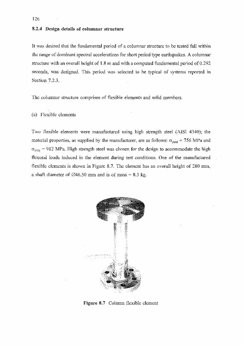
126
8.2.4 Design details of columnar structure
It was desired that the fundamental period of a columnar structure to be tested fall within
the range of dominant spectral accelerations for short period type earthquakes. A columnar
structure with an overall height of 1.8 m and with a computed fundamental period of 0.292
seconds, was designed. This period was selected to be typical of systems reported in
Section 7.2.3.
The columnar structure comprises of flexible elements and solid members.
(a) Flexible elements
Two flexible elements were manufactured using high strength steel (AISI 4340); the
material properties, as supplied by the manufacturer, are as follows: cryieid = 756 MPa and
crms = 912 MPa. High strength steel was chosen for the design to accommodate the high
flexural loads induced in the element during test conditions. One of the manufactured
flexible elements is shown in Figure 8.7. The element has an overall height of 280 mm,
a shaft diameter of 046.50 mm and is of mass= 8.3 kg.
Figure 8. 7 Column flexible element
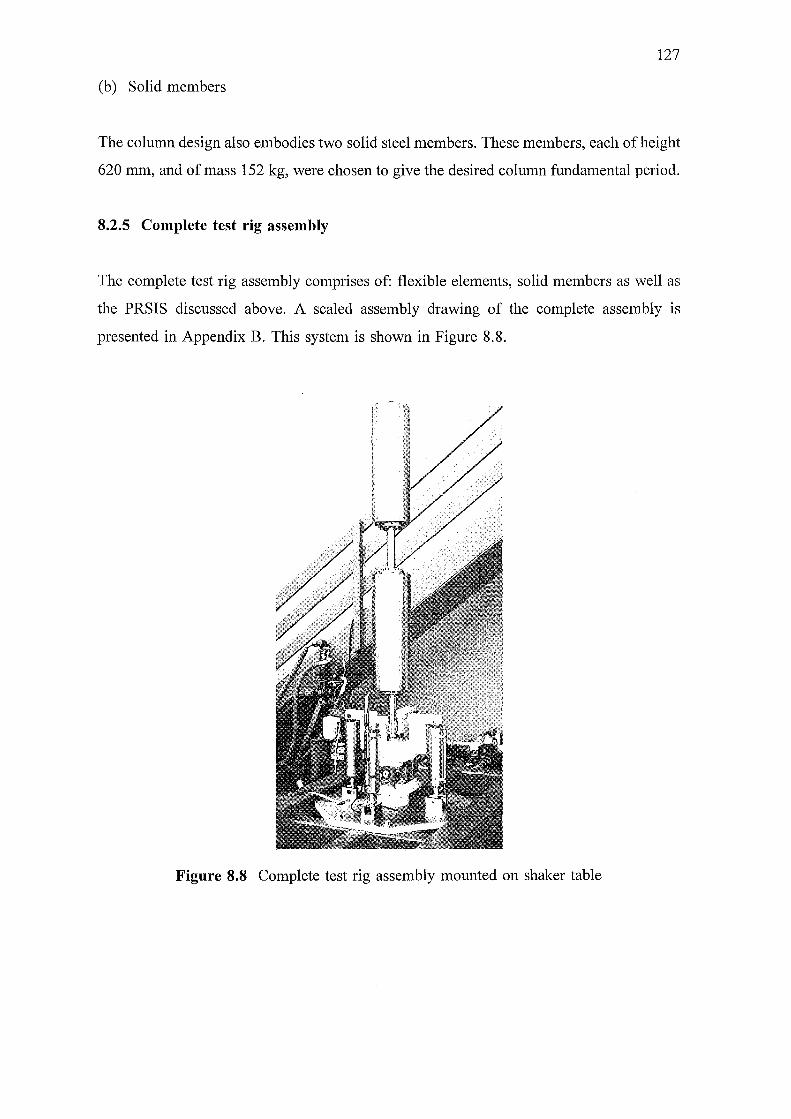
127
(b) Solid members
The column design also embodies two solid steel members. These members, each of height
620 mm, and of mass 152 kg, were chosen to give the desired column fundamental period.
8.2.5 Complete test rig assembly
The complete test rig assembly comprises of: flexible elements, solid members as well as
the PRSIS discussed above. A scaled assembly drawing of the complete assembly is
presented in Appendix B. This system is shown in Figure 8.8.
Figure 8.8 Complete test rig assembly mounted on shaker table
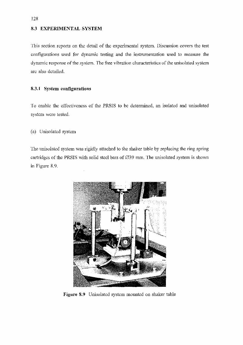
128
8.3 EXPERIMENTAL SYSTEM
This section reports on the detail of the experimental system. Discussion covers the test
configurations used for dynamic testing and the instrumentation used to measure the
dynamic response of the system. The free vibration characteristics of the unisolated system
are also detailed.
8.3.1 System configurations
To enable the effectiveness of the PRSIS to be determined, an isolated and unisolated
system were tested.
(a) Unisolated system
The unisolated system was rigidly attached to the shaker table by replacing the ring spring
cartridges of the PRSIS with solid steel bars of 039 mm. The unisolated system is shown
in Figure 8.9.
Figure 8.9 Unisolated system mounted on shaker table
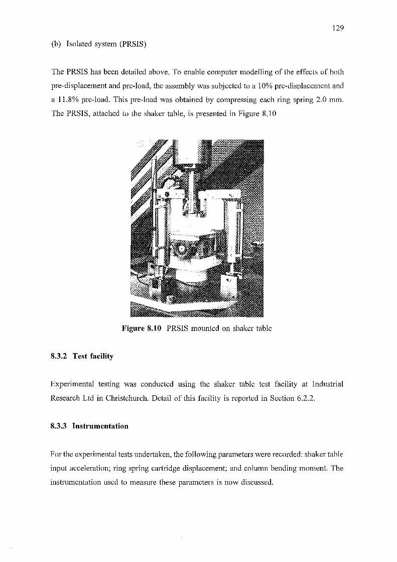
129
(b) Isolated system (PRSIS)
The PRSIS has been detailed above. To enable computer modelling of the effects of both
pre-displacement and pre-load, the assembly was subjected to a 10% pre-displacement and
a 11.8% pre-load. This pre-load was obtained by compressing each ring spring 2.0 mm.
The PRSIS, attached to the shaker table, is presented in Figure 8.10
Figure 8.10 PRSIS mounted on shaker table
8.3.2 Test facility
Experimental testing was conducted usmg the shaker table test facility at Industrial
Research Ltd in Christchurch. Detail of this facility is reported in Section 6.2.2.
8.3.3 Instrumentation
For the experimental tests undertaken, the following parameters were recorded: shaker table
input acceleration; ring spring cartridge displacement; and column bending moment. The
instrumentation used to measure these parameters is now discussed.
130
(a) Accelerometer
The shaker table input acceleration was measured using a Brtiel and Kjrer (B&K)
accelerometer, attached directly to the shaker table actuator. The accelerometer was
calibrated using a B&K accelerometer calibrator. An acceleration of 1.0 g gives a charge
amplifier output of 1.0 volt.
(b) Linear variable differential transducers
Two Schlumberger linear variable differential transducers (LVDT's) were used to measure
ring spring cartridge displacements. The LVDT's were attached to two orthogonal ring
spring cartridges, thus enabling displacements to be measured at 90° positions. Each L VDT
was calibrated to give a 1.0 volt output for a 10.0 mm ring spring displacement.
Attachment of the LVDT's to the ring spring cartridges is seen in Figure 8.10.
(c) Strain gauges
Bending moments induced in the column during dynamic loading were measured by
attaching a series of 1200 strain gauges at 90° intervals around the periphery of the shaft
section of the flexible element. This is seen in Figure 8.7; only the vertically mounted
gauges were used in this study. To minimise the influence of localised stress concentration
effects, the strain gauges were attached 30 mm away from the fillet radius at the junction
of the shaft section and the flange (Figure 8. 7).
Calibration of the strain gauges was undertaken by loading the flexible element in a
universal testing machine and measuring quasi-static strains using a six channel Kyowa
dynamic strain amplifier. Pairs of strain gauges, each fitted at 180° intervals on the flexible
element, were connected in a half bridge configuration. The gauges were connected to give
the summation of the strains for the axial load conditions experienced during testing in the
universal testing machine.
For applied loads up to 200 kN, the mean strain amplifier output voltage was 1.202
volts/1 000 llm strain. Using the sectional properties of the flexible element and Esteet = 21 0
GPa, the equivalent bending moment/volt output is 862.3 N-m/volt.
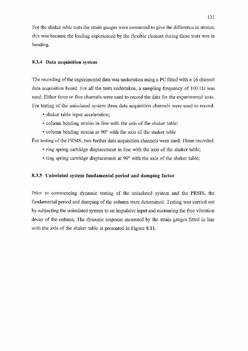
131
For the shaker table tests the strain gauges were connected to give the difference in strains;
this was because the loading experienced by the flexible element during these tests was in
bending.
8.3.4 Data acquisition system
The recording of the experimental data was undertaken using a PC fitted with a 16 channel
data acquisition board. For all the tests undertaken, a sampling frequency of 1 00 Hz was
used. Either three or five channels were used to record the data for the experimental tests.
For testing of the unisolated system three data acquisition channels were used to record:
• shaker table input acceleration;
• column bending strains in line with the axis of the shaker table;
• column bending strains at 90° with the axis of the shaker table
For testing of the PRSIS, two further data acquisition channels were used. These recorded:
• ring spring cartridge displacement in line with the axis of the shaker table;
• ring spring cartridge displacement at 90° with the axis of the shaker table;
8.3.5 Unisolated system fundamental period and damping factor
Prior to commencmg dynamic testing of the unisolated system and the PRSIS, the
fundamental period and damping of the colunm were determined. Testing was carried out
by subjecting the unisolated system to an impulsive input and measuring the free vibration
decay of the column. The dynamic response measured by the strain gauges fitted in line
with the axis of the shaker table is presented in Figure 8.11.
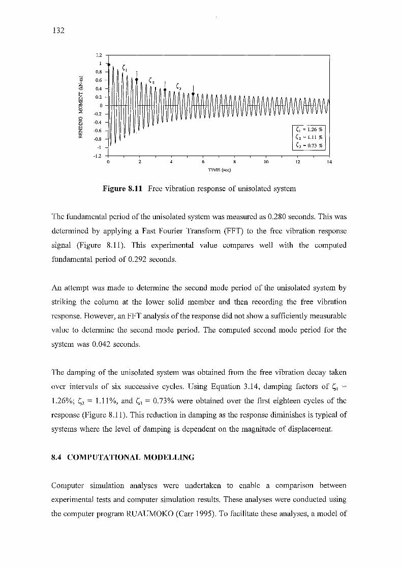
132
1.2
0.8 (1
I 0.6 (2
0.4 (3
I 0.2
0
-0.2 0 ~ -0.4
~ -0.6
-0.8
(1 = 1.26%
(2=1.11%
-1 (3 = 0.73 %
-1.2 0 2 4 6 8 10 12 14
TIME (sec)
Figure 8.11 Free vibration response of unisolated system
The fundamental period of the unisolated system was measured as 0.280 seconds. This was
determined by applying a Fast Fourier Transform (FFT) to the free vibration response
signal (Figure 8.11). This experimental value compares well with the computed
fundamental period of 0.292 seconds.
An attempt was made to determine the second mode period of the unisolated system by
striking the column at the lower solid member and then recording the free vibration
response. However, an FFT analysis of the response did not show a sufficiently measurable
value to determine the second mode period. The computed second mode period for the
system was 0.042 seconds.
The damping of the unisolated system was obtained from the free vibration decay taken
over intervals of six successive cycles. Using Equation 3.14, damping factors of s1 =
1.26%; s2 = 1.11 %, and s3 = 0.73% were obtained over the first eighteen cycles of the
response (Figure 8.11). This reduction in damping as the response diminishes is typical of
systems where the level of damping is dependent on the magnitude of displacement.
8.4 COMPUTATIONAL MODELLING
Computer simulation analyses were undertaken to enable a comparison between
experimental tests and computer simulation results. These analyses were conducted using
the computer program RUAUMOKO (Carr 1995). To facilitate these analyses, a model of
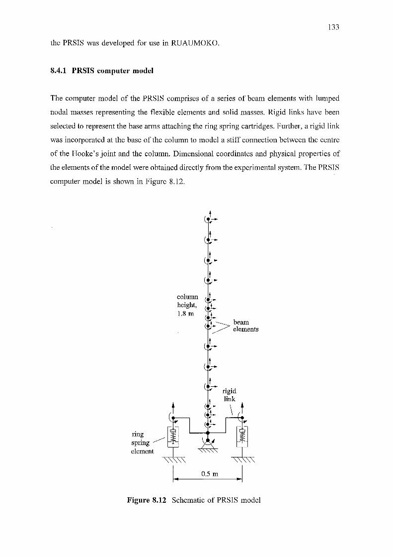
133
the PRSIS was developed for use in RUAUMOKO.
8.4.1 PRSIS computer model
The computer model of the PRSIS comprises of a series of beam elements with lumped
nodal masses representing the flexible elements and solid masses. Rigid links have been
selected to represent the base arms attaching the ring spring cartridges. Further, a rigid linlc
was incorporated at the base of the column to model a stiff connection between the centre
of the Hooke's joint and the column. Dimensional coordinates and physical properties of
the elements of the model were obtained directly from the experimental system. The PRSIS
computer model is shown in Figure 8.12.
column height, 1.8 ill
ring ~ spring~ -element
~~~
,_ !
0.5 ill .. I
Figure 8.12 Schematic of PRSIS model
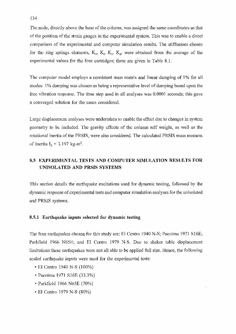
134
The node, directly above the base of the column, was assigned the same coordinates as that
of the position of the strain gauges in the experimental system. This was to enable a direct
comparison of the experimental and computer simulation results. The stiffnesses chosen
for the ring springs elements, K 0, Ki, K 1, Kd, were obtained from the average of the
experimental values for the four cartridges; these are given in Table 8.1.
The computer model employs a consistent mass matrix and linear damping of 1% for all
modes. 1% damping was chosen as being a representative level of damping based upon the
free vibration response. The time step used in all analyses was 0.0001 seconds; this gave
a converged solution for the cases considered.
Large displacement analyses were undertaken to enable the effect due to changes in system
geometry to be included. The gravity effects of the column self weight, as well as the
rotational inertia of the PRSIS, were also considered. The calculated PRSIS mass moment
of inertia I0 = 3.197 kg-m2•
8.5 EXPERIMENTAL TESTS AND COMPUTER SIMULATION RESULTS FOR
UNISOLATED AND PRSIS SYSTEMS
This section details the earthquake excitations used for dynamic testing, followed by the
dynamic response of experimental tests and computer simulation analyses for the unisolated
and PRSIS systems.
8.5.1 Earthquake inputs selected for dynamic testing
The four earthquakes chosen for this study are: El Centro 1940 N-S; Pacoima 1971 S16E;
Parkfield 1966 N65E; and El Centro 1979 N-S. Due to shaker table displacement
limitations these earthquakes were not all able to be applied full size. Hence, the following
scaled earthquake inputs were used for the experimental tests:
• El Centro 1940 N-S (100%)
• Pacoima 1971 S16E (33.3%)
• Parkfield 1966 N65E (70%)
• El Centro 1979 N-S (80%)

135
Acceleration inputs, recorded by an accelerometer attached to the shaker table, were used
as the RUAUMOKO input file. RUAUMOKO results for the PRSIS were output for:
(1) the bending moment at the node positioned at the strain gauges;
(2) the ring spring displacement.
For the unisolated system, column bending moment only was output.
Results of analyses for the El Centro 1940 N-S earthquake are detailed in the following
sections. The study considers the dynamic behaviour of the following four cases:
(i) the unisolated system built in at its base;
(ii) the unisolated system including the effects of subsystem flexibility;
(iii) the PRSIS mounted in line with the shaker table axis;
(iv) the PRSIS mounted at 45° with the shaker table axis.
8.5.2 Dynamic response of unisolated system
In this section the dynamic behaviour of the unisolated system, excluding, as well as
including, sub-system flexibility is detailed.
(a) Excluding sub-system flexibility
The system, mounted on the shaker table, was subjected to the El Centro 1940 N-S
earthquake. The shaker table acceleration, measured by the accelerometer attached to the
shaker table, is presented in Figure 8.13 (a). The bending moment time history experienced
by the flexible element during this excitation is shown in Figure 8.13 (b). These results are
plotted using the same time base.
For the computer simulation analysis, the computer model considered the column to be
built in at its base, that is, the base node of the column was constrained in the x, y and 8
directions. The fundamental period of this system, given by the computer model, is 0.292
seconds. This compares with a value of 0.280 seconds obtained experimentally.
The computer simulation bending moment time history using the measured shaker table
acceleration is presented in Figure 8.13 (c).
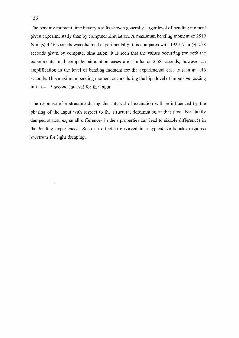
136
The bending moment time history results show a generally larger level of bending moment
given experimentally than by computer simulation. A maximum bending moment of 2519
N-m@ 4.46 seconds was obtained experimentally; this compares with 1920 N-m@ 2.58
seconds given by computer simulation. It is seen that the values occurring for both the
experimental and computer simulation cases are similar at 2.58 seconds, however an
amplification in the level of bending moment for the experimental case is seen at 4.46
seconds. This maximum bending moment occurs during the high level of impulsive loading
in the 4 - 5 second interval for the input.
The response of a structure during this interval of excitation will be influenced by the
phasing of the input with respect to the structural deformation at that time. For lightly
damped structures, small differences in their properties can lead to sizable differences in
the loading experienced. Such an effect is observed in a typical earthquake response
spectrum for light damping.
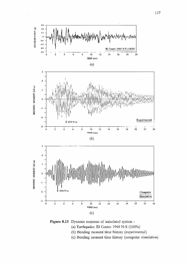
0.3
:§ 0.2
; 0.1
0
-0.1
-0.2
~ -0.3
-0.4
3
2
0
-1
-2
-3
3
2
s ~ ;
0
~ (!)
I -1
-2
-3
0 2 4 6 8
-
-
-
-
- A~~ AA
- T ~ ~p
-
-
-
10
TIME (sec)
(a)
12
El Centro 1940 N-S (100%)
14 16 18
137
20
-- 2519 N-m
Experimental
0 2 4 6 8 10 12 14 16 18 20 22 24
TIME (sec)
(b)
Computer
Simulation
0 2 4 6 8 10 12 14 16 18 20 22 24
TIME (sec)
(c)
Figure 8.13 Dynamic response of unisolated system -
(a) Earthquake: El Centro 1940 N-S (100%)
(b) Bending moment time history (experimental)
(c) Bending moment time history (computer simulation)
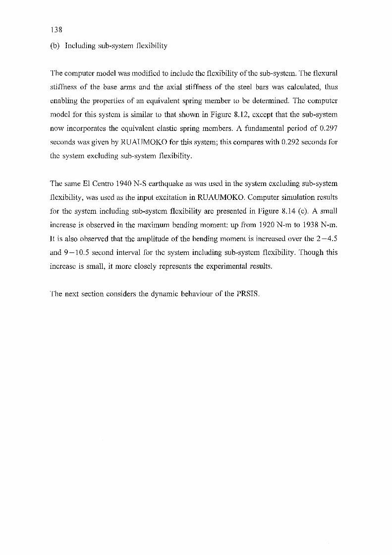
138
(b) Including sub-system flexibility
The computer model was modified to include the flexibility of the sub-system. The flexural
stiffness of the base arms and the axial stiffness of the steel bars was calculated, thus
enabling the properties of an equivalent spring member to be determined. The computer
model for this system is similar to that shown in Figure 8.12, except that the sub-system
now incorporates the equivalent elastic spring members. A fundamental period of 0.297
seconds was given by RUAUMOKO for this system; this compares with 0.292 seconds for
the system excluding sub-system flexibility.
The same El Centro 1940 N-S earthquake as was used in the system excluding sub-system
flexibility, was used as the input excitation in RUAUMOKO. Computer simulation results
for the system including sub-system flexibility are presented in Figure 8.14 (c). A small
increase is observed in the maximum bending moment: up from 1920 N-m to 1938 N-m.
It is also observed that the amplitude of the bending moment is increased over the 2-4.5
and 9- 10.5 second interval for the system including sub-system flexibility. Though this
increase is small, it more closely represents the experimental results.
The next section considers the dynamic behaviour of the PRSIS.
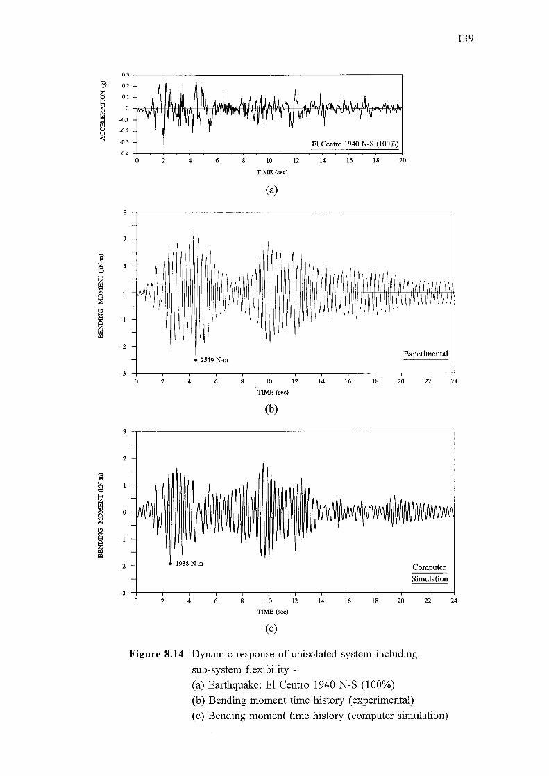
:§
I u <t!
0.3
0.2
0.1
0
-0.1
-0.2
-0.3 El Centro 1940 N-S (100%) -0.4
0 2 4 6 8 10 12 14 16 18 20
TIME (sec)
(a)
3
-
2 -
-
-
-IM I AA
! ~ ~~~M~~~ ~!!!!!~~!~~~Ill T\/lr II~
- ~ ~ ~ ~ ~ ~ ~ ~ ~~ ~ ~1 ~ ~ II~ ~I! ~ I -
0
-1
-
-2 -
- 2519 N-m Experimental
-3 0 2 4 6 8 10 12 14 16 18 20 22 24
TIME (sec)
(b)
3 ~------------------------------------------------~
2
-1
-2 Computer
Simulation
-3 ,_---,---.---.---.----.---,---,---.----.---,---,--~ 0 2 4 6 8 10 12 14 16 18 20
TIME (sec)
(c)
Figure 8.14 Dynamic response of unisolated system including
sub-system flexibility -
(a) Earthquake: El Centro 1940 N-S (100%)
(b) Bending moment time history (experimental)
22
(c) Bending moment time history (computer simulation)
24
139
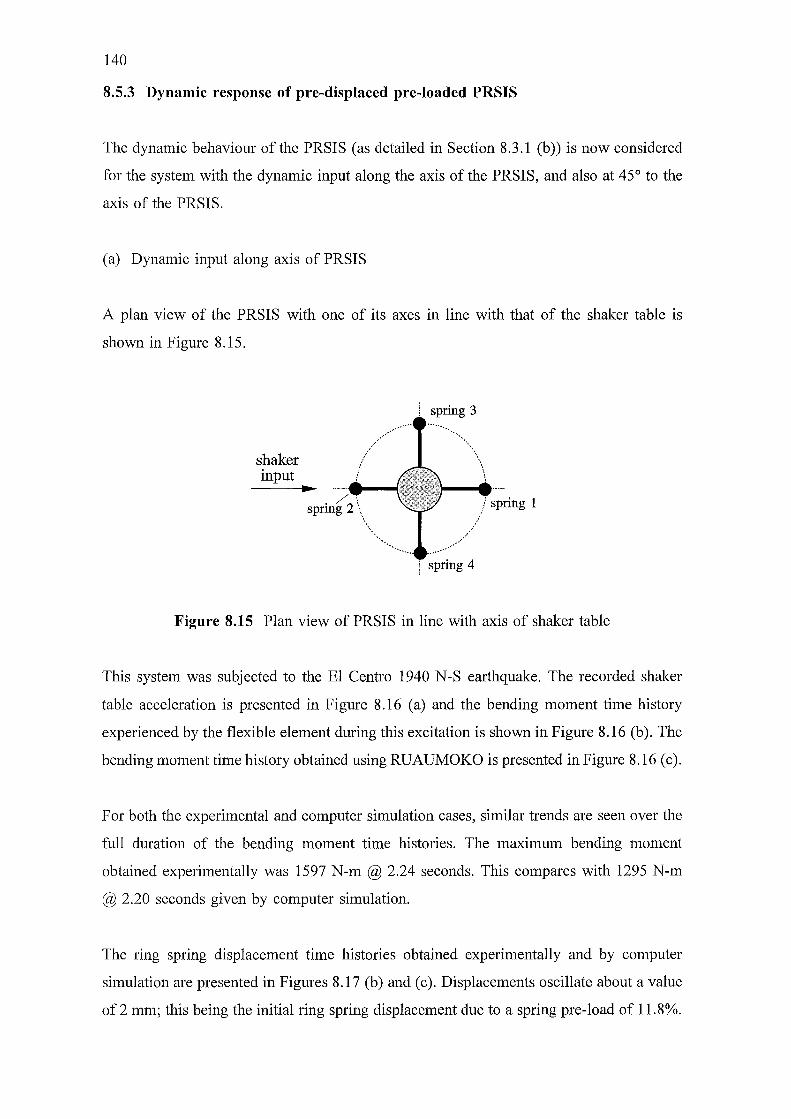
140
8.5.3 Dynamic response of pre-displaced pre-loaded PRSIS
The dynamic behaviour of the PRSIS (as detailed in Section 8.3.1 (b)) is now considered
for the system with the dynamic input along the axis of the PRSIS, and also at 45° to the
axis of the PRSIS.
(a) Dynamic input along axis of PRSIS
A plan view of the PRSIS with one of its axes in line with that of the shaker table is
shown in Figure 8.15.
shaker input
. /2\ sprmg \\· ..
'•, ···· ...
spring 3
/spring 1
. ... --·/
spring 4
Figure 8.15 Plan view of PRSIS in line with axis of shaker table
This system was subjected to the El Centro 1940 N-S earthquake. The recorded shaker
table acceleration is presented in Figure 8.16 (a) and the bending moment time history
experienced by the flexible element during this excitation is shown in Figure 8.16 (b). The
bending moment time history obtained using RUAUMOKO is presented in Figure 8.16 (c).
For both the experimental and computer simulation cases, similar trends are seen over the
full duration of the bending moment time histories. The maximum bending moment
obtained experimentally was 1597 N-m @ 2.24 seconds. This compares with 1295 N-m
@ 2.20 seconds given by computer simulation.
The ring spring displacement time histories obtained experimentally and by computer
simulation are presented in Figures 8.17 (b) and (c). Displacements oscillate about a value
of 2 mm; this being the initial ring spring displacement due to a spring pre-load of 11.8%.
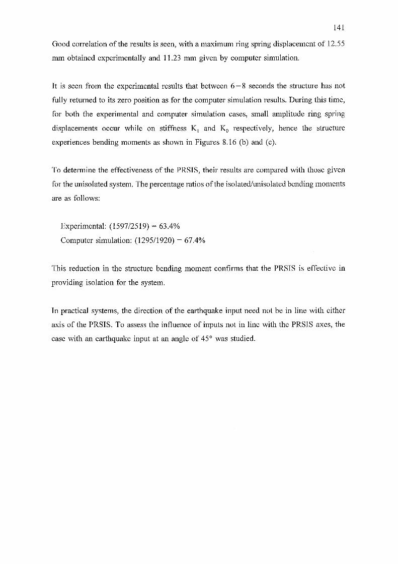
141
Good correlation of the results is seen, with a maximum ring spring displacement of 12.55
mm obtained experimentally and 11.23 mm given by computer simulation.
It is seen from the experimental results that between 6-8 seconds the structure has not
fully returned to its zero position as for the computer simulation results. During this time,
for both the experimental and computer simulation cases, small amplitude ring spring
displacements occur while on stiffness K1 and Ko respectively, hence the structure
experiences bending moments as shown in Figures 8.16 (b) and (c).
To determine the effectiveness of the PRSIS, their results are compared with those given
for the unisolated system. The percentage ratios of the isolated/unisolated bending moments
are as follows:
Experimental: (1597/2519) = 63.4%
Computer simulation: (1295/1920) = 67.4%
This reduction in the structure bending moment confirms that the PRSIS is effective in
providing isolation for the system.
In practical systems, the direction of the earthquake input need not be in line with either
axis of the PRSIS. To assess the influence of inputs not in line with the PRSIS axes, the
case with an earthquake input at an angle of 45° was studied.
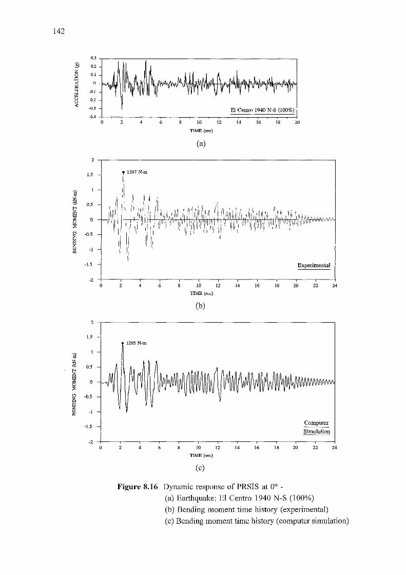
142
0.3 --,--------,----------------------,
0.2
0.1
0 ...WWHH
-0.1
-0.2
-0.3 El Centro 1940 N-S (100%) -0.4 -!-~~~~-~~~~~~~-~-.-=:::;::==;::::::;::::=::;::==;:::::;:::::::.j
0 2 4 6 8 10
TIME (sec)
(a)
12 14 16 18 20
2 ,-----------------------------.
1.5 1597 N-m
0.5
0
-0.5
-1
-1.5 Experimental
0 2 4 6 8 10 12 14 16 18 20 22 24
TIME (sec)
(b)
2 .-----------------------------.
1.5
0.5
0
-0.5
-1
-1.5
1295 N-m
Computer
Simulation
-2 -r--.--.---.--.--,---.--.---,--,,--,---.-~ 0 2 4 6 8 10 12 14 16 18 20 22 24
TIME (sec)
(c)
Figure 8.16 Dynamic response of PRSIS at oo -(a) Earthquake: El Centro 1940 N-S (100%)
(b) Bending moment time history (experimental)
(c) Bending moment time history (computer simulation)
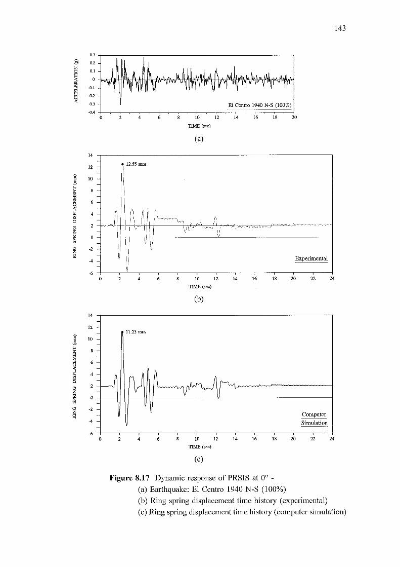
0.3
3 0.2
~ 0.1
~ 0
-0.1
tl -0.2 (.)
...:: -0.3
-0.4
14
12
1 10
~ 8
6 (.)
~ 4 ~ Ci
C!J 2
~ 0
"' C!J -2
~ -4
-6
14
12
1 10
I 8
6
~ 4 ~ Ci
C!J 2
~ 0
"' C!J -2
~ -4
-6
0 2 4
- 12.55mm --------
=~Nj __ -~I ------
0 2 4
--- 11.23 mm
-------
( p) -
-
-----0 2 4
6 8 10
TIME (sec)
(a)
12
~"~·~~"\_, v·"\ A c/1 A
\j\1" '\J'-r._l v __ ._
6 8 10 12
TIME (sec)
(b)
El Centro 1940 N-S (100%)
14 16 18 20
.•. ·v
--
Experimental
14 16 18 20 22 24
A (\.1"\ In "--'vv ~\/
Computer
Simulation
6 8 10 12 14 16 18 20 22 24
TIME (sec)
(c)
143
Figure 8.17 Dynamic response of PRSIS at oo -(a) Earthquake: El Centro 1940 N-S (100%)
(b) Ring spring displacement time history (experimental)
(c) Ring spring displacement time history (computer simulation)
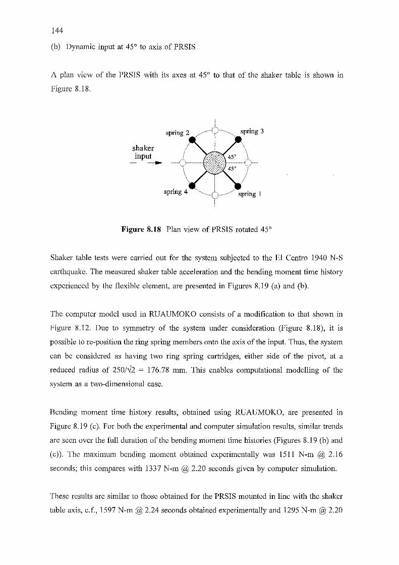
144
(b) Dynamic input at 45° to axis of PRSIS
A plan view of the PRSIS with its axes at 45° to that of the shaker table is shown in
Figure 8.18.
shaker input ....
; ;
spring 2 ,---·······-<;>·········... spring 3
'·· ..... {"···:--··· · ..... spring 1 spring 4
i
Figure 8.18 Plan view of PRSIS rotated 45°
Shaker table tests were carried out for the system subjected to the El Centro 1940 N-S
earthquake. The measured shaker table acceleration and the bending moment time history
experienced by the flexible element, are presented in Figures 8.19 (a) and (b).
The computer model used in RUAUMOKO consists of a modification to that shown in
Figure 8.12. Due to symmetry of the system under consideration (Figure 8.18), it is
possible to re-position the ring spring members onto the axis of the input. Thus, the system
can be considered as having two ring spring cartridges, either side of the pivot, at a
reduced radius of 250/.Y2 = 176.78 mm. This enables computational modelling of the
system as a two-dimensional case.
Bending moment time history results, obtained using RUAUMOKO, are presented in
Figure 8.19 (c). For both the experimental and computer simulation results, similar trends
are seen over the full duration of the bending moment time histories (Figures 8.19 (b) and
(c)). The maximum bending moment obtained experimentally was 1511 N-m @ 2.16
seconds; this compares with 1337 N-m @ 2.20 seconds given by computer simulation.
These results are similar to those obtained for the PRSIS mounted in line with the shaker
table axis, c.f., 1597 N-m@ 2.24 seconds obtained experimentally and 1295 N-m@ 2.20

145
seconds given by computer simulation.
The ring spring displacement time histories, obtained experimentally and by computer
simulation for the PRSIS rotated 45°, are presented in Figures 8.20 (b) and (c).
Displacement results for ring spring cartridges 1 and 3, both fitted with LVDT's, are seen
to be in good agreement (Figure 8.20 (b)). This suggests that rocking of the system
occurred about an axis orthogonal to the shaker input. Good correlation is seen for the
experimental and computer simulation results, with maximum ring spring displacements
of 7.20 mm and 7.71 mm obtained experimentally and 6.63 mm given by computer
simulation.
It is seen from the computer simulation results (Figure 8.20 (c)) that the structure returns
near to its initial position of 2 mm; its final displacement being 1. 79 mm. This effect of
a small offset from the original displacement is common to pre-displaced pre-loaded
systems.
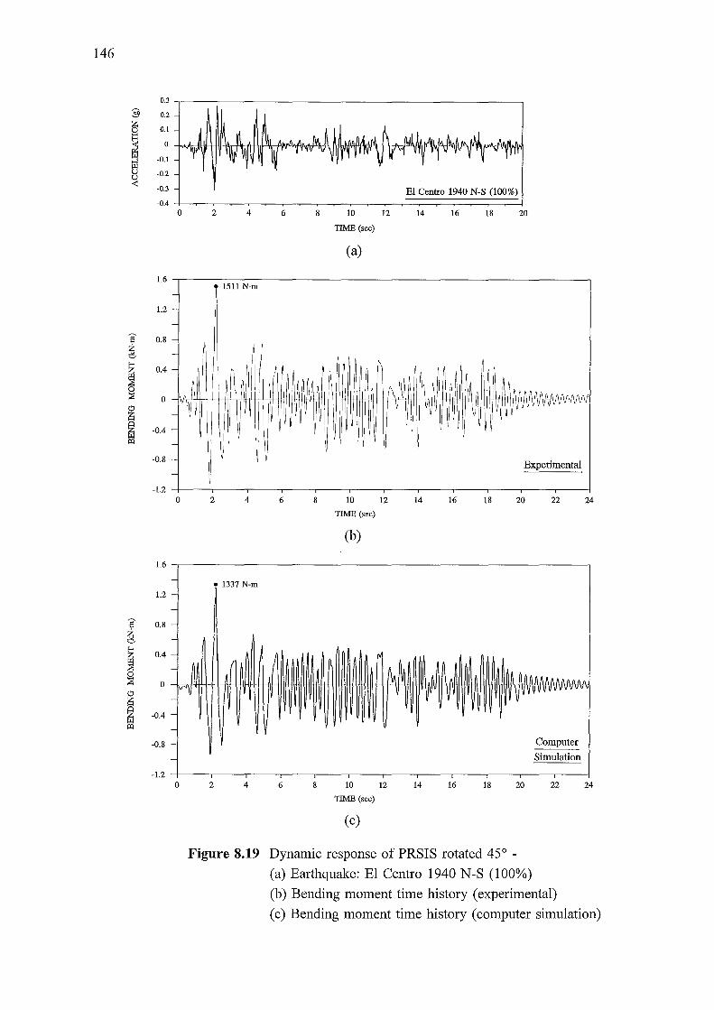
146
0.3
3 0.2
a 0.1
~ 0
-0.1
eJ -0.2 (.)
4! -0.3
-0.4
1.6
1.2
s.: ~
0.8
~ 0.4
0 ::s 0
@
ffi -0.4 >0
-0.8
-1.2
1.6
1.2
s.: 0.8
~
~ 0.4
~ 0
@
ffi -0.4 >0
-0.8
-1.2
0 2 4
1511 N-m ---
-
-
-
" ~~ -
~ - \ --
--
0 2 4
-1337 N-m
-----
- ~~ r
~"""~ --
-
-
-
0 2 4
6 8
Ill
6 8
J I~
6 8
10
TIME (sec)
(a)
10
TIME (sec)
(b)
10
TIME (sec)
(c)
El Centro 1940 N-S (100%)
12 14 16 18 20
r\N \H II II~ ~ ~AAAAAAAAAAAAA ' v V\J I~ 'VI ~I · ~ v v v v v v v v
Experimental
12 14 16 18 20 22 24
rJ ~~ ~~I IL~ }'1 lh AAAAAAIIAA/\111111 v ~v vv I~ vvvvvvvv• •
Computer
Simulation
12 14 16 18 20 22 24
Figure 8.19 Dynamic response of PRSIS rotated 45° -
(a) Earthquake: El Centro 1940 N-S (100%)
(b) Bending moment time history (experimental)
(c) Bending moment time history (computer simulation)
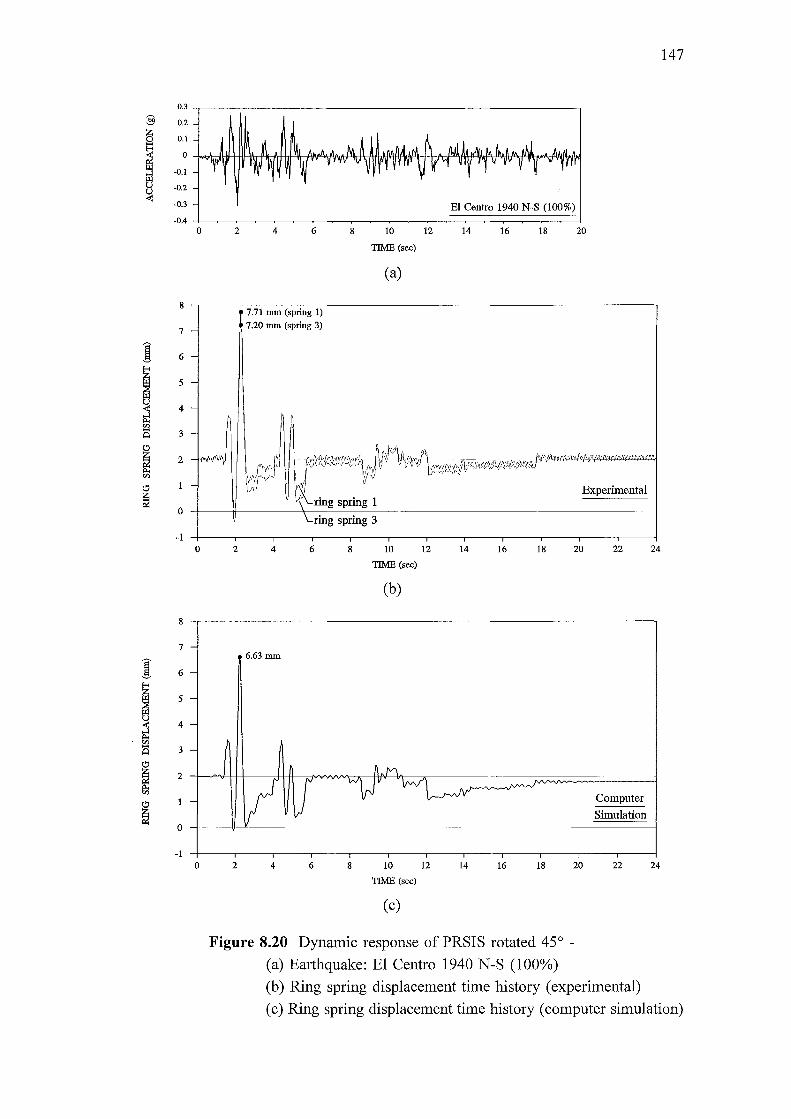
0.3
:§ 0.2
! 0.1
0
-0.1
u -0.2 ~
-0.3
-0.4
8
7
j 6
I 5
~ 4
s 3
" ~ 2
~
" ~ 0
-1
8
7
j 6
~ 5
4
f!l 3 Q
~ 2
" ~ 0
-1
0 2
-
-
-
-
-
- Nnfi
-
0 2
0 2
4 6
7.71 mm (spring 1) 7.20 mm (spring 3)
8 10
TIME (sec)
(a)
El Centro 1940 N-S (100%)
12 14 16 18 20
t!f~ ~ J"""" "" ! rl'\n. .•. A JV\N'-I'-1'-\AJ\~ ~ tncv ~~~(~#v
\;0- ring spring 1 Experimental
~--
\...ring spring 3
4 6 8 10 12 14 16 18 20 22 24
TIME (sec)
(b)
Computer
Simulation
4 6 8 10 12 14 16 18 20 22 24
TIME (sec)
(c)
147
Figure 8.20 Dynamic response of PRSIS rotated 45° -
(a) Earthquake: El Centro 1940 N-S (100%)
(b) Ring spring displacement time history (experimental)
(c) Ring spring displacement time history (computer simulation)
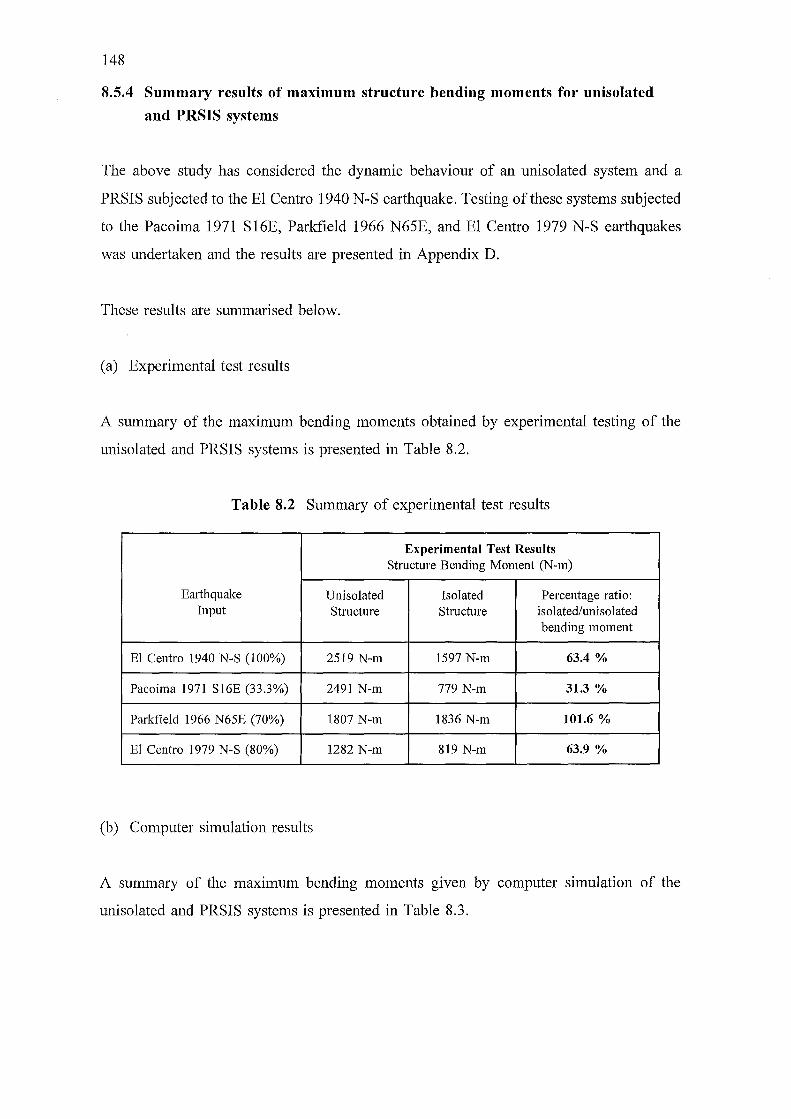
148
8.5.4 Summary results of maximum structure bending moments for unisolated
and PRSIS systems
The above study has considered the dynamic behaviour of an unisolated system and a
PRSIS subjected to the El Centro 1940 N-S earthquake. Testing of these systems subjected
to the Pacoima 1971 S16E, Parkfield 1966 N65E, and El Centro 1979 N-S earthquakes
was undertaken and the results are presented in Appendix D.
These results are summarised below.
(a) Experimental test results
A summary of the maximum bending moments obtained by experimental testing of the
unisolated and PRSIS systems is presented in Table 8.2.
Table 8.2 Summary of experimental test results
Experimental Test Results Structure Bending Moment (N-m)
Earthquake Unisolated Isolated Percentage ratio: Input Structure Structure isolated/unisolated
bending moment
El Centro 1940 N-S (100%) 2519 N-m 1597 N-m 63.4%
Pacoima 1971 S16E (33.3%) 2491 N-m 779 N-m 31.3%
Parkfield 1966 N65E (70%) 1807 N-m 1836 N-m 101.6 %
El Centro 1979 N-S (80%) 1282 N-m 819 N-m 63.9%
(b) Computer simulation results
A summary of the maximum bending moments given by computer simulation of the
unisolated and PRSIS systems is presented in Table 8.3.
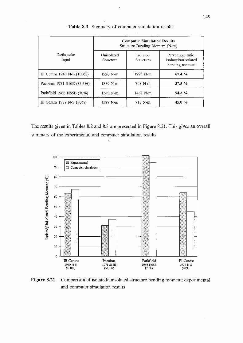
149
Table 8.3 Summary of computer simulation results
Computer Simulation Results Structure Bending Moment (N-m)
Earthquake Unisolated Isolated Percentage ratio: Input Structure Structure isolated/unisolated
bending moment
El Centro 1940 N-S (100%) 1920 N-m 1295 N-m 67.4%
Pacoima 1971 S16E (33.3%) 1889 N-m 708 N-m 37.5%
Parkfield 1966 N65E (70%) 1549 N-m 1461 N-m 94.3%
El Centro 1979 N-S (80%) 1597 N-m 718 N-m 45.0%
The results given in Tables 8.2 and 8.3 are presented in Figure 8.21. This gives an overall
summary of the experimental and computer simulation results.
100
D Experimental 90 0 Computer simulation
...--. 80 ~ ._, 'l:l s 70 0 ::s bJ) 60
;@ ~ 50 ~
13 1;! 40 0 ·El ~ 30
1;! -0 20 ;a
10
0
El Centro Pacoima Parkfield El Centro 1940 N-S 1971 S16E 1966 N65E 1979 N-S
(100%) (33.3%) (70%) (80%)
Figure 8.21 Comparison of isolated/unisolated structure bending moment: experimental
and computer simulation results
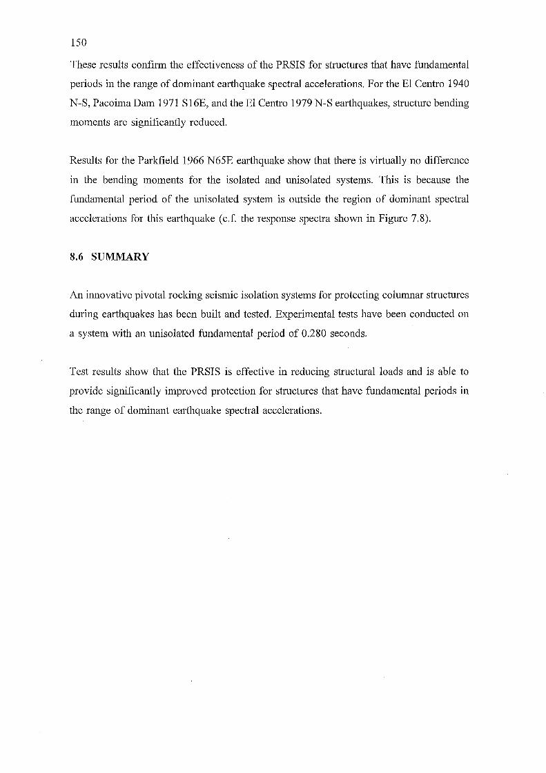
150
These results confirm the effectiveness of the PRSIS for structures that have fundamental
periods in the range of dominant earthquake spectral accelerations. For the El Centro 1940
N-S, Pacoima Dam 1971 S16E, and the El Centro 1979 N-S earthquakes, structure bending
moments are significantly reduced.
Results for the Parkfield 1966 N65E earthquake show that there is virtually no difference
in the bending moments for the isolated and unisolated systems. This is because the
fundamental period of the unisolated system is outside the region of dominant spectral
accelerations for this earthquake (c.f. the response spectra shown in Figure 7.8).
8.6 SUMMARY
An innovative pivotal rocking seismic isolation systems for protecting columnar structures
during earthquakes has been built and tested. Experimental tests have been conducted on
a system with an unisolated fundamental period of 0.280 seconds.
Test results show that the PRSIS is effective in reducing structural loads and is able to
provide significantly improved protection for structures that have fundamental periods in
the range of dominant earthquake spectral accelerations.
151
Chapter 9
CONCLUSIONS AND RECOMMENDATIONS
9.1 CONCLUSIONS
This research project has examined the characteristics, design requirements, and dynamic
response of ring spring systems. Based on this and a comprehensive study of the aseismic
design methods used in engineering design, an innovative seismic isolation system
incorporating ring springs was developed and subsequently tested. The key findings of this
research are presented below.
• Aseismic design methods can be broadly classified into two principal techniques:
strength design and response control. Of the response control techniques, seismic
isolation is a simple yet effective method of reducing structural loads during
earthquakes.
e Ring springs are friction devices capable of absorbing large amounts of input energy;
these devices have application where a high level of damping is required. Practical
use of ring springs requires: lubrication of the ring elements; either internal or
external guidance of the spring stack, and a minimum pre-tension force of at least
5-10% of the maximum load capacity of the spring. Based upon their free vibration
response, practical ring springs have damping factors of between 11.9% and 17.6%.
• Experimental testing of a prototype bi-directional ring spring cartridge showed its
hysteresis characteristics comprise of four stiffnesses: Ko, Ki, K 1, and Kd.
• Mass/ring spring systems may be pre-displaced, pre-loaded, or pre-displaced pre
loaded. The theoretical free vibration response of pre-displaced mass/ring spring
systems showed that motion proceeds around the hysteresis diagram until settling onto
the origin stiffness (Ko); for pre-loaded systems, motion proceeds about an
equilibrium line equal to the pre-load force. A zone is set up within which motion
eventually settles.
152
• The theoretical behaviour of pre-displaced mass/ring spring systems was verified by
experimental tests. These test results showed that the ring spring hysteresis
characteristics behaved in accordance with those given by quasi-static testing.
• Ring springs are possible candidates for use in earthquake-resistant applications. They
are deemed especially suitable for use in rocking/stepping seismic isolation systems.
To investigate this option, a pivotal rocking seismic isolation system (PRSIS) was
developed.
• Computer analyses for a range of isolated and unisolated systems subjected to six
different earthquake inputs, showed that PRSIS 's can significantly reduce structural
loads during short period type earthquakes - in some cases by a factor of between
three and four.
• Shaker table tests conducted on a PRSIS showed that the design is effective in
reducing structural loads during short period type earthquakes.
• An application seen as ideal for use of PRSIS' s is in protecting high voltage electrical
equipment during earthquakes. Though this is one specific situation, the isolation
system has potential application to protecting a wide range of columnar type
structures during earthquakes; for larger systems ground support of the structure
weight may be required. Possible candidates include multi-storey buildings, chimneys,
towers, as well as other similarly proportioned structures.
9.2 RECOMMENDATIONS FOR FURTHER RESEARCH
The work outlined in this thesis has established a basis from which further research can
be undertaken. Suggested areas for additional work are as follows.
• Design guidelines outlining steps in the selection of suitable ring springs for specific
applications are required. Design charts may be useful for presenting this information.
• RUAUMOKO is at present being expanded to enable dynamic modelling of non-

153
linear three-dimensional systems. When fully developed, a study should be undertaken
to investigate the effect of simultaneously applying two horizontal earthquake
components to a structure. Further, inputs not in line with the axes of the PRSIS
should be considered.
• A study is required that compares the performance of PRSIS's incorporating ring
springs with other types of isolation systems and devices, for example, Belleville
washers. RUAUMOKO may be a suitable software package for undertaking computer
simulation analyses.
• The option of utilising a PRSIS consisting of three cartridges attached to the base
should be investigated; this design could provide economic advantages over a system
that uses four cartridges. Also, rather than a single support for the pivot mechanism,
multi-support configurations should be explored. These systems may be suitable for
support of larger structures.

154

155
REFERENCES
ANDRIONO, T., and CARR, A.J. (1991) Reduction and distribution of lateral seismic inertia forces on base isolated multistorey structures, Bull. N.Z. Nat. Soc. Earthq. Eng., Vol 24, No. 3, pp 225-237.
BERGMAN, D.M., and HANSON, R.D. (1988) Characteristics of mechanical dampers, Ninth World Conf. Earthq. Eng., Japan, Vol 5, pp 815-820.
BERRY, W.R. (1961) Spring design- A practical treatment, Emmott & Company Ltd, London, pp 262-266.
BOARDMAN, P.R., WOOD, B.J., and CARR, A.J. (1983) Union House -A cross braced structure with energy dissipators, Bull. N.Z. Nat. Soc. Earthq. Eng., Vol 16, No. 2, pp 83-97.
BOWEN, A.A.D. (1981) Mechanical Springs, Oxford University Press, Oxford, pp 34-39.
BRANDOW, G.E. and LEEDS, D.J. (1980) Reconnaissance Report: Imperial Country, California, earthquake, Oct. 15, 1979, Earthq. Eng. Research Institute, 194 pp.
BUCKLE, I.G. (1985) New Zealand seismic base isolation concepts and their applications to nuclear engineering, Nuclear Eng. and Design, Vol 84, No.3, pp 313-326.
BUCKLE, I.G. (1989) Recent developments in isolation hardware, seismic engineering: Research and practice, Proc. of the Sessions Related to Seismic Eng. at Structures Congress '89, San Francisco, California, ASCE, pp 789-798.
BUCKLE, I. G., and MAYES, R.L. (1990) Seismic isolation: Histmy, application, and pe!formance- A world overview, Earthq. Spectra, Vol 6, No. 2, pp 161-202.
CARR, A.J. (1995) Ruaumoko computer program libra!)', Dept. of Civil Eng., University of Canterbury, 132 pp.
CASPE, M.S. (1984) Base isolationfi·om earthquake hazards- An idea whose time has come!, Eighth World Conf. Earthq. Eng., California, Vol 5, pp 1031-1038.
CHARLESON, A.W., WRIGHT, P.D., and SKINNER, R.I. (1987) Wellington central police station- Base isolation of an essential facility, Pacific Conf. Earthq. Eng., New Zealand, Vol 2, pp 377-388.
COAD, J.N.O., and PHAM, L.T. (1993) The earthquake strengthening of high voltage electrical equipment, Proc. IPENZ Annual Conf., Hamilton, pp 321-330.
CORMACK, L.G. (1988) The design and construction of the major bridges on the Mangaweka rail deviation, IPENZ Trans., Vol 15, liCE, pp 16-23.
COUSINS, W.J., ROBINSON, W.H., and McVERRY, G.H. (1991) Recent developments in devices for seismic isolation, Pacific Conf. Earthq. Eng., New Zealand, Vol 2, pp 221-232.
CRAIG, R.R. Jr. (1981) Structural dynamics, an introduction to computer methods, John Wiley & Sons, New York, 527 pp.
DELFOSSE, G.C. (1977) The GAPEC system: A new highly effective aseismic system, Sixth World Conf. Earthq. Eng., India, Vol2, pp 1135-1140.
DELFOSSE, G.C. (1980) Full earthquake protection through base isolation system, Seventh World Conf. Earthq. Eng., Turkey, Vol 8, pp 61-68.
DOWRICK, D.J., BABOR, J., COUSINS, W.J., and SKINNER, R.I. (1991) Seismic isolation of a printing press in Wellington, New Zealand, Pacific Conf. Earthq. Eng., New Zealand, Vol 3, pp 35-44.

156
ENDSLEY, L.E. (1933) Draft gear springs- past and present, Railway Mech. Engineer, Vol 107, No. 7, pp 253-255.
ERASMUS, L. ( 1988) Ring springs on holding-down bolts for seismic energy dissipation, IPENZ Trans., Vol 15, No. 2/CE, pp 41-47.
ESHLEMAN, R.L., and RAO, P.N. (1969) The response of mechanical shock isolation elements to high rate input loading, Shock and Vib. Bull., Vol 40, No. 5, pp 217-234.
ESHLEMAN, R.L. (1972) Dynamic response of a ring spring, Shock and Vib. Bull., Vol42, No.4, pp 7-14.
FUJITA, T. (1985) Earthquake isolation technology for industrial facilities - Research, development and applications in Japan, Bull. N.Z. Nat. Soc. Earthq. Eng., Vol 18, No. 3, pp 224-249.
FUJITA, S., FUJITA, T., SASAKI, Y., FUJIMOTO, S., NARIKAWA, N., and TSURUYA, C. (1988) Earthquake isolation systems for buildings of industrial facilities using various types of damper, Ninth World Conf. Earthq. Eng., Japan, Vol 5, pp 797-802.
GODDEN, W.G., ASLAM, M., and SCALISE, D.T. (1980) Seismic isolation of an electron microscope, Seventh World Conf. Earthq. Eng., Turkey, Vol 8, pp 69-76.
GROSS, S. (1966) Calculation and design of metal springs, Chapman and Hall, London, pp 193-211.
HARTZELL, S. (1979) Analysis of the Bucharest strong ground motion record for the March 4, 1977 Romanian earthquake, Bull. Seism. Soc. Am., Vol 69, No. 2, pp 513-530.
HIGASHINO, M., AIZA WA, S., and HA YAMIZU, Y. (1988) The study of base isolation system for actual use, Ninth World Conf. Earthq. Eng., Japan, Vol 5, pp 705-710.
HILL, K.E. (1992) Aseismic design: A review of methods, developments and applications, Dept. of Mech. Eng., University of Canterbury, 53 pp.
HILL, K.E. (1993) Fundamental dynamic characteristics of ring springs, Proc. Vibrations Assoc. of N.Z. Annual Conf., Christchurch, pp 182-90.
HILL, K.E. (1994a) Design aspects for incmporating ring springs into practical systems, Proc. IPENZ Annual Conf., Nelson, Vol 1, pp 80-84.
HILL, K.E. (1994b) Dynamic properties of ring springs for use as seismic energy dissipators, Pro c. N.Z. Nat. Soc. Earthq. Eng. Annual Conf., Wairakei, pp 96-101.
HILL, K.E. (1994c) Dynamic energy absmption utilising ring springs, Int. Mech. Eng. Congress and Exhibition., Perth, Australia, Vol 3, pp 207-212.
HILL, K.E. (1994d) Characteristics and dynamic response of ring spring systems, IPENZ Trans., Vol 21, No 1/EMCh, pp 6-9.
HILL, K.E. (1995a) A prototype ring spring cartridge for mitigating transient and seismic inputs, Proc. IPENZ Annual Conf., Palmerston North, Vol 2, pp 145-150.
HILL, K.E. (1995b) Application of ring springs to seismic isolation systems, Proc. N.Z. Nat. Soc. Earthq. Eng. Annual Conf., Rotorua, pp 21-27.
Hill, K.E. (1995c) Experimental testing and computer simulation of a prototype ring spring cartridge subject to shock excitation, IPENZ Trans., Vol 22, No. 1/EMCh, pp 10-15.
Hill, K.E. (1995d) Seismic isolation of columnar structures utilising ring springs, Pacific Conf. on Earthq. Eng., Melbourne, Australia, Vol1, pp 101-110.

157
HISANO, M., KAWAMURA, S., KITAZAWA, K., and NAGASHIMA, I. (1988) Study on a sliding-type base isolation system-tri-axial shaking table test and its simulation, Ninth World Conf. Earthq. Eng., Japan, Vol 5, pp 741-746.
HITCHCOCK, H.C. (1969) Electrical equipment and earthquakes, NZ Eng., Vol 24, No. 1, pp 3-14.
HITCHCOCK, H. C. (1973) The specification of earthquake resistance for electricity system equipment, Bull. N.Z. Nat. Soc. Earthq. Eng., Vol 6, No. 4, pp 178-207.
HOUSNER, G.W. and TRIFUNAC, M.D. (1967) Analysis of accelerograms- Parlifield earthquake, Bull. Seism. Soc. Am., Vol 57, No. 6, pp 1193-1220.
HOUSNER, G.W. and JENNINGS, P.C. (1972) The San Fernando California earthquake, Earthq. Eng. Struct. Dyn., Vol 1, pp 5-31.
HROVAT, D., BARAK, P., and RABINS, M. (1983) Semi-active versus passive or active tuned mass dampers for structural control, Journal of Eng. Mechanics, Vol109, No.3, pp 691-705.
HUFFMANN, G. (1980) Spring-damper systems for the support of structures to prevent earthquake damage, Seventh World Conf. Earthq. Eng., Turkey, Vol 8, pp 167-168.
ISHIGURO, Y., KOSUDA, N., MAEHARA, Y., and SHIMODA, I. (1977) Shock absorbers with viscous shear resistance and its experiment, Sixth World Conf. Earthq. Eng., India, Vol 3, pg 3243.
IZUMI, M. (1988) State-of-the-art report: Base isolation and passive seismic response control, Ninth World Conf. Earthq. Eng., Japan, Vol 8, pp 385-396.
IZUMI, M., andY AMAHARA, H. (1988) Comparisons between earthquake response characteristics of baseisolated and ordinal)! buildings, Ninth World Conf. Earthq. Eng., Japan, Vol 5, pp 687-692.
KARNOPP, D., CROSBY, M.J., and HARWOOD, R.A. (1974) Vibration control using semi-active force generators, Journal of Eng. for Industry, Vol 96, No.2, pp 619-626.
KASHIWAZAKI, A., TANAKA, M., and TOKUDA N. (1988) Shaking test of seismic isolation floor system by using 3-dimensional isolator, Ninth World Conf. Earthq. Eng., Japan, Vol 5, pp 845-850.
KAWAMURA, S., KITAZAWA, K., HISANO, M., and NAGASHIMA, I. (1988) Study on a sliding-type base isolation system-system composition and element properties, Ninth World Conf. Earthq. Eng., Japan, Vol 5, pp 735-740.
KELLY, J.M., and BEUCKE, K.E. (1983) A fi·iction damped base isolation system with fail-safe characteristics, Earthq. Eng. and Struct. Dyn., Vol II, pp 33-56.
KELLY, J.M. (1986) Aseismic base isolation: Review and bibliography, Soil Dyn. and Earthq. Eng., Vol 5, No. 4, pp 202-216.
KITAMURA, H., FUJITA, T., TERAMOTO, T., and KIHARA, H. (1988) Design and analysis of a tower structure with a tuned mass damper, Ninth World Conf. Earthq. Eng., Japan, Vol 8, pp 4I5-420.
KITTA, T., KODERA, 1., UJIIE, K., and TADA, H. (1973) A new type shock absorber and its effects on the response of the bridge to the earthquake, Fifth World Conf. Earthq. Eng., Rome, Vol 1, pp 1397-I400.
KOBORI, T., KANA YAMA, H., and KAMAGATA, S. (1988) A proposal of new anti-seismic structure with active seismic response control system- dynamic intelligent building, Ninth World Conf. Earthq. Eng., Japan, Vol 8, pp 465-470.
LEE, D.M., and MEDLAND, I.C. (1978) Base isolation -An historical development, and the influence of higher mode responses, Bull. N.Z. Nat. Soc. Earthq. Eng., Vol I1, No. 4, pp 219-233.

158
MCKAY, G.R., CHAPMAN, H.E., and KIRKCALDIE, D.K. (1990) Seismic isolation: New Zealand applications, Earthq. Spectra, Vol 6, No. 2, pp 203-222.
MATHEWSON, C.D., andDA VEY, R.A. (1980) Precast concrete braced frames incorporating load-limiting energy-dissipating devices in an earthquake resistant building, Seventh World Conf. Earthq. Eng., Turkey, Vol 7, pp 349-356.
MAYES, R.L., JONES, L.R., KELLY, T.E., and BUTTON, M.R. (1984) Design guidelines for base-isolated buildings with energy dissipators, Earthq. Spectra, Vall, No. 1, pp 41-74.
MAYES, R.L., JONES, L.R., and KELLY, T.E. (1990) The economics of seismic isolation in buildings, Emthq. Spectra, Vol 6, No. 2, pp 245-263.
MEGGET, L.M. (1978) Analysis and design of a base-isolated reinforced concreteji·ame building, Bull. N.Z. Nat. Soc. Eatihq. Eng., Vol 11, No. 4, pp 245-254.
MILLER, R.K., MASRI, S.F., DEHGHANY AR, T.J., and CAUGHEY, T.K. (1988) Active vibration control of large civil structures, Journal of Eng. Mechanics, Vol 114, No. 9, pp 1542-1570.
MOSTAGHEL, N. (1986) Resilient-fi·iction base isolator (R-FBI), Proc. of a Seminar and Workshop on Base Isolation and Passive Energy Dissipation, Applied Technology Council Report ATC-17, pp 221-230.
NAGASHIMA, I., KAWAMURA, S., KITAZAWA, K., and HISANO, M. (1988) Study on a sliding-type base isolation system-multi-dimensional response analysis, Ninth World Conf. Earthq. Eng., Japan, Vol 5, pp 747-752.
NEWMARK, N.M. (1962) A method of computation for structural dynamics, Trans. ASCE, Vol 127, No. 1, pp 1406-1435.
NORTON, J.A., KING, A.B., BULL, D.K., CHAPMAN, H.E., McVERRY, G.H., LARKIN, T.J., and SPRING, K.C. (1994) Northridge earthquake reconnaissance report, Bull. N.Z. Nat. Soc. Earthq. Eng., Vol 27, No. 4, pp 235-344.
OAKESHOTT, G.B. (1975) San Fernando, California, earthquake of9 FebruaJ)i 1971, California Division of Mines and Geology, Bull. 196, 463 pp.
PALL, A.S. (1986) Energy-dissipation devices for aseismic design of buildings, Proc. of a Seminar and Workshop on Base Isolation and Passive Energy Dissipation, Applied Technology Council Report ATC-17, pp 241-250.
PARK, R. (1987) Development of structural design procedures for earthquake resistance in New Zealand, IPENZ Trans., Vol 14, liCE, pp 22-32.
PARK, R., BILLINGS, I.J., CLIFTON, G.C., COUSINS, J., FILLIATRAULT, A., JENNINGS, D.N., JONES, L.C.P., PERRIN, N.D., ROONEY, S.L., SINCLAIR, J., SPURR, D.D., TANAKA, H., and WALKER, G. (1995) The Hyogo-ken Nanbu earthquake of 17 Janumy 1995, Bull. N.Z. Nat. Soc. Earthq. Eng., Vol 28, No. 1, pp 1-98.
PENDER, M.J., and ROBERTSON, T.W. (1987) Edgecumbe earthquake: Reconnaissance report, Bull. N.Z. Nat. Soc. Earthq. Eng., Vol 20, No. 3, pp 201-249.
PHAM, L.T. (1988) A base-isolation design using spherically-ended rollers and telescopic shock absorbers, Bull. N.Z. Nat. Soc. Earthq. Eng., Vol 21, No. 2, pp 135-139.
PHAM, T., and HOBY, P. (1991) The design, testing and applications of Belleville washers as a damping device for seismic protection of electrical equipment, Pacific Conf. on Emihq. Eng., New Zealand, Vol 3, pp 381-391.
POOLE, R.A., and CLENDON, J.E. (1992) NZ parliament buildings: Seismic protection by base isolation, Bull. N.Z. Nat. Soc. Earthq. Eng., Vol 25, No. 3, pp 147-160.

159
RANI, P., and KUMAR, A. (1980) Control of seismic effect on switchyard equipments by vibration isolation system, Seventh World Conf. Earthq. Eng., Turkey, Vol 8, pp 77-84.
RING FEDER GmbH, (1925) Stoj3verzehrende Vorrichtung, Patentschrift Nr. (Patent No.) 4204 73, Klasse 4 7a, Gruppe 17 (in German).
RINGFEDER GmbH, (1984) Friction springs, Ringfeder in Mech. Eng., Report R55E, 52 pp.
ROBINSON, W.H., and GREENBANK, L.R. (1975) Properties of an extrusion energy absorber, Bull. N.Z. Nat. Soc. Earthq. Eng., Vol 8, No.3, pp 187-191.
ROBINSON, W.H., and GREENBANK, L.R. (1976) An extrusion energy absorber suitable for the protection of structures during an earthquake, Earthq. Eng. and Struct. Dyn., Vol 4, pp 251-259.
ROBINSON, W.H., and TUCKER, A.G. (1977) A lead-rubber shear damper, Bull. N.Z. Nat. Soc. Earthq. Eng., Vol 10, No.3, pp 151-153.
ROBINSON, W.H., and TUCKER, A.G. (1981) Test results for lead-rubber bearings for W.M Clayton building, Toe Toe bridge, and Waiotukupuna bridge, Bull. N.Z. Nat. Soc. Emthq. Eng., Vol 14, No. 1, pp 21-33.
ROBINSON, W.H. (1982) Lead-rubber hysteretic bearing suitable for protecting structures during earthquakes, Earthq. Eng. and Struct. Dyn., Vol 10, pp 593-604.
ROBINSON, W.H., HASKELL, T.G., and GANNON, C.R. (1995) Testing of seismic isolation systems, Proc. N.Z. Nat. Soc. Earthq. Eng. Annual Conf., Rotorua, pp 1-6.
RUTLEDGE, A., PHAM, T., LAFFERTY, M., ROBERTSON, R., and RANBY, P. (1984) Vibration tests and the installation of belleville washers on tokaanu switchyard equipment, NZ Electricity Research Report R/52/84.
RUTLEDGE, A.L. (1988) Earthquake damage at Edgecumbe and Kawerau Electricorp substations in the Bay of Plenty earthquake on 2 March 1987, Bull. N.Z. Nat. Soc. Earthq. Eng., Vol 21, No.4, pp 247-254.
SAFI, B.F., PHAM, L.T., and BUSBY, M.J. (1989) High voltage circuit breaker supported on a base isolating tripod for earthquake protection, Bull. N.Z. Nat. Soc. Earthq. Eng., Vol 22, No. 3, pp 145-154.
SEED, H.B., ROMO, M.P., SUN, J.I., JAIME, A. and LYSMER, J. (1988) The Mexico earthquake of September 19, 1985- Relationships between soil conditions and earthquake ground motions, Earthq. Spectra, Vol4, No.4, pp 687-729.
SHARPE, R.D. (1974) The seismic response of inelastic structures, PhD thesis, Dept. of Civil Eng., University of Canterbury, 126 pp.
SHARPE, R.D., and SKINNER, R.I. (1983) The seismic design of an industrial chimney with rocking base, Bull. N.Z. Nat. Soc. Earthq. Eng., Vol 16, No.2, pp 98-106.
SHEPHERD, R., and ERASMUS, L.A. (1988) Ring spring energy dissipators in seismic resistant structures, Ninth World Conf. Earthq. Eng., Japan, Vol 5, pp 767-772.
SIMPSON, C. (1970) Ring springs can solve problems, Engineering, pp 580-581.
SKINNER, R.I., KELLY, J.M., and HEINE, A.J. (1975) Hysteretic dampers for earthquake-resistant structures, Earthq. Eng. Struct. Dyn., Vol 3, pp 287-296.
SKINNER, R.I., TYLER, R.G., HEINE, A.J., and ROBINSON, W.H. (1980) Hysteretic dampers for the protection of structures from earthquakes, Bull. N.Z. Nat. Soc. Earthq. Eng., Vol 13, No. 1, pp 22-36.
SKINNER, R.I., ROBINSON, W.H. and McVERRY, G. (1993) An introduction to seismic isolation, John Wiley and Sons, New York, 354 pp.

160
SLADEK, J.R., and KLINGNER, R.E. (1980) Using tuned-mass dampers to reduce seismic response, Seventh World Conf. Earthq. Eng., Turkey, Vol 7, pp 265-271.
SOONG, T.T. (1988) State-of-the-art review: Active structural control in civil engineering, Eng. Structures, Vol 10, No. 2, pp 74-84.
SRITHARAN, S., and DOWRICK, D.J. (1994) Response of/ow-rise buildings to moderate ground shaking, particularly the May 1990 Weber earthquake, Bull. N.Z. Nat. Soc. Earthq. Eng., Vol27, No.3, pp 205-221.
TAJIRIAN, F.F., and KELLY, J.M. (1989) Seismic isolation of nuclear plants: A world overview, seismic engineering: research and practice, Proceedings of the Sessions Related to Seismic Eng. at Structures Congress '89, San Francisco, California, ASCE, pp 799-808.
TAKAI, H., UNO, T., and NAGAI, K. (1988) Study on thefi·iction damper as the device of a base isolation system, Ninth World Conf. Earthq. Eng., Japan, Vol 5, pp 803-808.
TANAKA, M., TOKUDA, N., YOKOZAWA, J., AIZAWA, K., KASHIWAZAKI, A., KOBAYASHI, M., MATSUMOTO, S., and ENOMOTO, T. (1989) Development of earthquake andmicrotremor isolation floor system utilizing air springs and laminated rubber bearings, IHI Engineering (English Ed.) Vol22, No.2, pp 47-52.
TEZCAN, S., CIVI, A., and HOFFMANN, G. (1980) Spring-dashpot vibration isolators against earthquakes, Seventh World Conf. Earthq. Eng., Turkey, Vol 8, pp 53-60.
THIEL, C.C. JR., ELSESSER, E., JONES, L., KELLY, T., BERTERO, V., FILIPPOU, F., and MCCANN, R. (1986) A seismic energy absorbing cladding system: A feasibility study, Proc. of a Seminar and Workshop on Base Isolation and Passive Energy Dissipation, Applied Technology Council Report ATC-17, pp 25 I -260.
TRIFUNAC, M.D. and BRUNE, J.N. (1970) Complexity of energy release during the Imperial Valley, California, earthquake of 1940, Bull. Seism. Soc. Am., Vol 60, No. 1, pp 137-160.
TYLER, R.G. (1977a) Dynamic tests on PTFE sliding layers under earthquake conditions, Bull. N.Z. Nat. Soc. Eatihq. Eng., Vol 10, No. 3, pp 129-138.
TYLER, R.G. (1977b) Damping in building structures by means ofPTFE slidingjoints, Bull. N.Z. Nat. Soc. Earthq. Eng., Vol 10, No.3, pp 139-142.
TYLER, R.G. (1983) PreliminalJ' tests on an energy absorbing element for braced structures under earthquake loading, Bull. N.Z. Nat. Soc. Earthq. Eng., Vol 16, No. 3, pp 201-212 ..
TYLER, R.G. (1985a) Further notes on a steel energy-absorbing element for bracedfi·ameworks, Bull. N.Z. Nat. Soc. Earthq. Eng., Vol 18, No. 3, pp 270-279.
TYLER, R.G. (1985b) Test on a brake lining damperfor structures, Bull. N.Z. Nat. Soc. Earthq. Eng., Vol 18, No. 3, pp 280-284.
TYLER, R.G. (1991) Rubber bearings in base-isolated structures- A summmJ' paper, Bull. N.Z. Nat. Soc. Earthq. Eng., Vol 24, No. 3, pp 251-274.
WAHL, A.M. (1963) Mechanical springs, McGraw-Hill, New York, 2nd Ed, pp 204-210.
WIKANDER, O.R. (1924) Characteristics of the ring spring, American Machinist, Vol 60, No. 7, pp 253-254.
WII<ANDER, O.R. (1926) The ring spring, Mech. Eng., ASME, Vol 48, No. 2, pp 139-143.
ZAYAS, V.A., LOW, S.S., and MAHIN, S.A. (1990) A simple pendulum technique for achieving seismic isolation, Earthq. Spectra, Vol 6, No.2, pp 317-333.
ZELLER, E. (1973) Dynamic tests on an actual building mounted with a new damper system, Fifth World Conf. Eatihq. Eng., Rome, Vol2, pp 1517-1520.
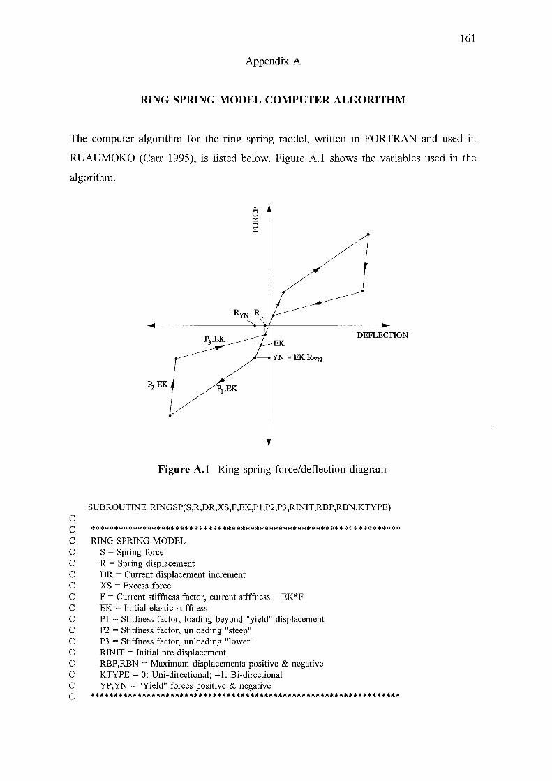
161
Appendix A
RING SPRING MODEL COMPUTER ALGORITHM
The computer algorithm for the ring spring model, written in FORTRAN and used in
RUAUMOKO (Carr 1995), is listed below. Figure A.1 shows the variables used in the
algorithm.
DEFLECTION
- YN=EK.RYN
P2 .EK
Figure A.l Ring spring force/deflection diagram
SUBROUTINE RINGSP(S,R,DR,XS,F,EK,P 1 ,P2,P3,RINIT,RBP,RBN,KTYPE) c c ****************************************************************** C RING SPRING MODEL C S = Spring force C R = Spring displacement C DR = Current displacement increment C XS = Excess force C F =Current stiffness factor, current stiffness = EK*F C EK = Initial elastic stiffness C PI = Stiffness factor, loading beyond "yield" displacement C P2 = Stiffness factor, unloading "steep" C P3 = Stiffness factor, unloading "lower" C RINIT = Initial pre-displacement C RBP,RBN =Maximum displacements positive & negative C KTYPE = 0: Uni-directional; =1: Bi-directional C YP,YN = "Yield" forces positive & negative c ******************************************************************

162
INTEGER KTYPE CS REAL S,R,DR,XS,F,EK,Pl,P2,P3,RINIT,RBP,RBN CS REAL RO,Rl,RYP,RYN,YP,YN,RNEW,TOL CD DOUBLE PRECISION S,R,DR,XS,F,EK,Pl,P2,P3,RINIT,RBP,RBN CD DOUBLE PRECISION RO,Rl,RYP,RYN,YP,YN,RNEW,TOL
c DATA TOL/0.0001/
xs = 0.0 IF(ABS(DR).LE.O.O) GO TO 100 RINIT = ABS(RINIT) RO = ((P3-Pl)/(l.O-P3)+Pl)*RINIT Rl = -RO RYP = Pl *RINIT RYN = -RYP YP = EK*RYP YN = -YP XS = S+F*EK*DR RNEW =R+DR IF(RNEW.GT.RO) THEN
IF(RBP.GT.RYP) THEN IF(DR.GT.O.O) THEN
IF(XS.GE.YP+Pl *EK*(RNEW-RYP)-TOL) THEN F = Pl S = YP+Pl *EK*(RNEW-RYP)
ELSEIF(RNEW.GE.RO.AND.RNEW.LE.RYP) THEN F = 1.0 S =EK*RNEW
ELSE F = P2 S = S+DR*P2*EK
ENDIF ELSE
IF(XS.LE.EK*RO+P3*EK*(RNEW-RO)+TOL) THEN F = P3 S = EK*RO+P3*EK*(RNEW-RO)
ELSEIF(RNEW.GE.RO .AND.RNEW.LE.RYP) THEN F = 1.0 S =EK*RNEW
ELSE F = P2 S = S+P2*EK*DR
ENDIF ENDIF
ELSE IF(RNEW.GE.RYP) THEN
F = Pl S = YP+Pl *EK*(RNEW-RYP)
ELSE F = 1.0 S = EK*RNEW
ENDIF ENDIF
ELSEIF(RNEW.LT.Rl.AND.KTYPE.GT.O) THEN IF(RBN.L T.RYN) THEN
IF(DR.L T.O.O) THEN IF(XS.LE.YN+Pl *EK*(RNEW-RYN)+TOL) THEN
F = Pl S = YN+Pl *EK*(RNEW-RYN)

c
ELSEIF(RNEW.LE.Rl.AND.RNEW.GE.RYN) THEN F = 1.0 S =EK*RNEW
ELSE F =P2 S = S+DR*EK*P2
ENDIF ELSE
IF(XS.GE.EK*Rl+P3*EK*(RNEW-Rl)-TOL) THEN F = P3 S = EK*Rl+P3*EK*(RNEW-Rl)
ELSEIF(RNEW.LE.Rl.AND.RNEW.GE.RYN) THEN F = 1.0 S =EK*RNEW
ELSE F =P2 S = S+DR *P2*EK
END IF ENDIF
ELSE IF(RNEW.LE.RYN) THEN
F = Pl S = YN+Pl *EK*(RNEW-RYN)
ELSE F = 1.0 S = EK*RNEW
END IF ENDIF
ELSE IF(RNEW.GE.O.O.OR.(RNEW.LT.O.O.AND.KTYPE.GT.O)) THEN
F = 1.0 S = EK*RNEW
ELSEIF(RNEW.LT.O.O) THEN F = 0.0 s = 0.0
ENDIF ENDIF R=RNEW XS = XS-S RBP = MAX(R,RBP) RBN = MIN(R,RBN)
100 RETURN END
163

164

Appendix B
SCALED GENERAL ASSEMBLY DRAWINGS
This appendix presents four scaled general assembly drawings. These are:
Drawing No. 1: Bi-directional ring spring cartridge
Drawing No. 2: Uni-directional ring spring cartridge
Drawing No. 3: Pivotal rocking seismic isolation system (PRSIS)
Drawing No. 4: Complete test rig assembly
165
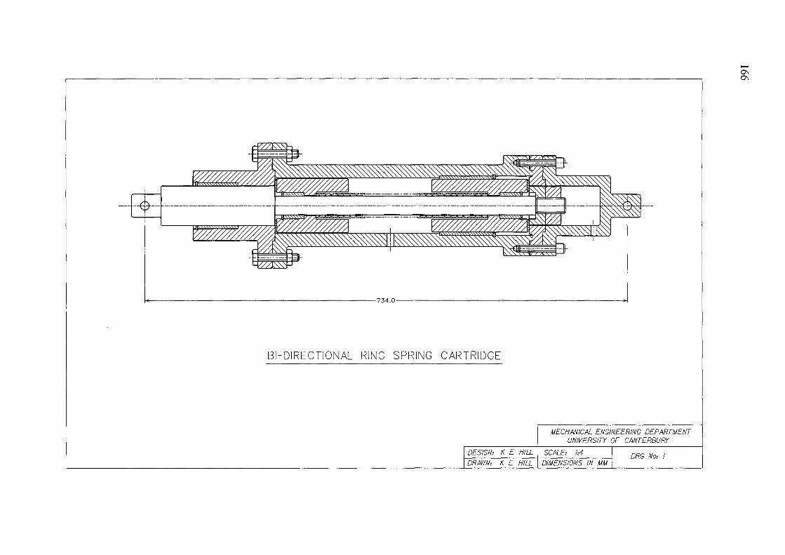
~-----------------------------------------------734.0------------------------------------------------~
BI-DIRECTIONAL RING SPRING CARTRIDGE
MECHANICAL ENGINEERING DEPARTMENT UNIVERSITY OF CANTERBURY
DESIGN: K E HILL I SCALE: 1:4 DRG No: I DRAWN: K E HILL I DIMENSIONS IN MM
........ 0\ 0\
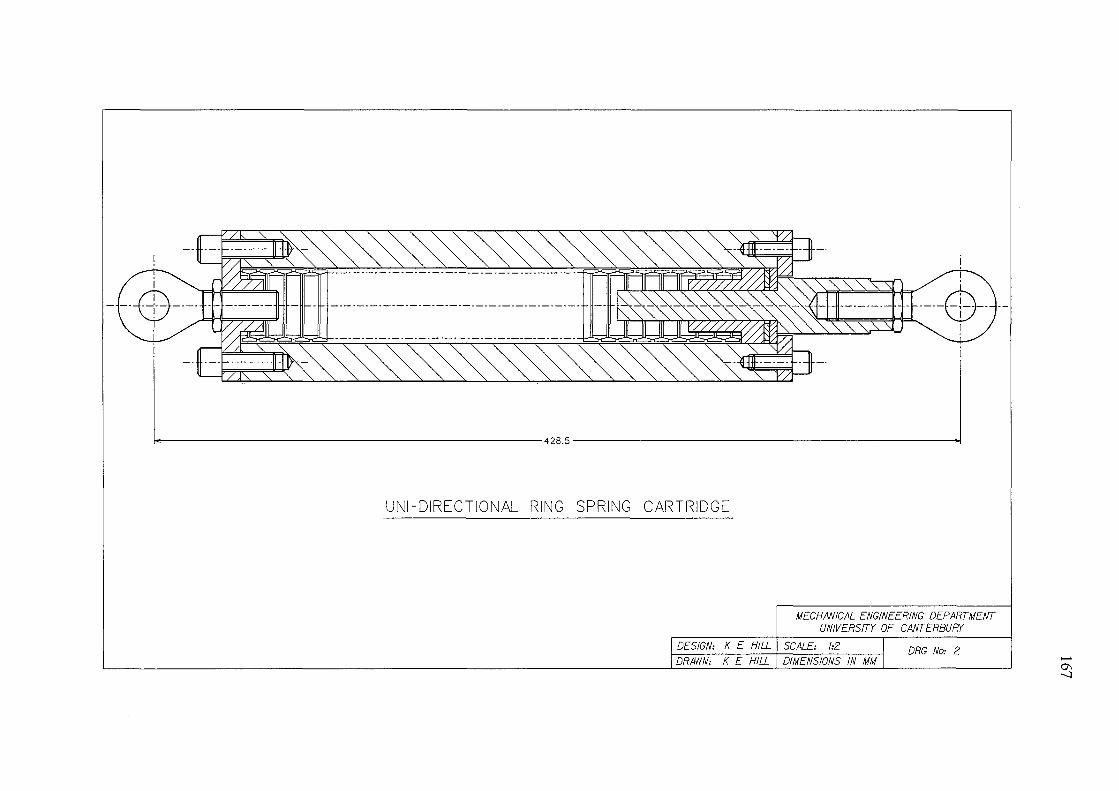
~--------------------------------------------------------428.5--------------------------------------------------------~
UNI-DIRECTIONAL RING SPRING CARTRIDGE
MECHIWICAL ENGINEERING DEPARTMENT UNIVERSITY OF CANTERBURY
DESIGN: K E HILL I SCALE: 1:2 DRG Na: 2 DRAWN: K E HILL I DIMENSIONS IN MM .........
0\ -....)
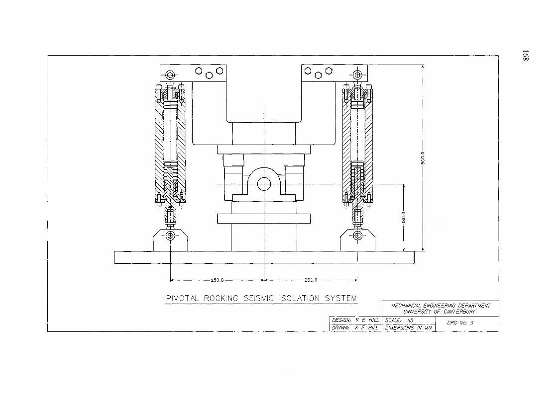
-4- I
-@)-0 0 0 0 0 0
I
1-<--------250.0 250.0 -------""1
PIVOTAL ROCKING SEISMIC ISOLATION SYSTEM
I 0 0 ':2
0
0 0 <il
MECHANICAL ENGINEERING DEPARTMENT UNIVERSITY OF CANTERBURY
DESIGN: K E HILL I SCALE: 1:5 DRG No: 3 DRAWN: K E HILL I DIMENSIONS IN MM
......... o-, 00
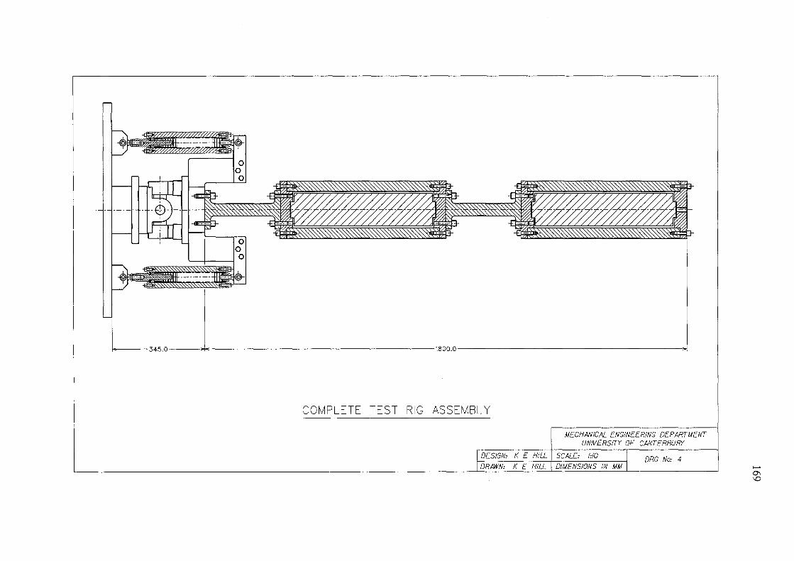
L3<5.0 >800.0-------------------------+1
COMPLETE TEST RIG ASSEMBLY
MECHANICAL ENGINEERING DEPARTMENT UNIVERSITY OF CANTERBURY
DESIGN: K E HILL I SCALE: 1:10 DRG No: 4 DRAWN: K E HILL I DIMENSIONS IN MM >-'
0'\ \D

170
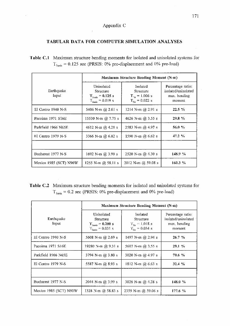
171
Appendix C
TABULAR DATA FOR COMPUTER SIMULATION ANALYSES
Table C.l Maximum structure bending moments for isolated and unisolated systems for T1unis = 0.125 sec (PRSIS: 0% pre-displacement and 0% pre-load)
Maximum Structure Bending Moment (N-m)
Unisolated Isolated Percentage ratio: Earthquake Structure Structure isolated/unisolated
Input Tlunis = 0.125 S Tlis = 1.006 S max. bending T2unis = 0.019 S T21, = 0.022 S moment
El Centro 1940 N-S 5406 N-m @ 2.61 s 1214 N-m@ 2.91 s 22.5%
Pacoima 1971 S16E 15530 N-m @ 7.75 s 4626 N-m@ 3.55 s 29.8%
Parkfield 1966 N65E 4612 N-m @ 4.21 s 2583 N-m @ 4.97 s 56.0%
El Centro 1979 N-S 3366 N-m @ 6.82 s 1590 N-m @ 6.62 s 47.2%
Bucharest 1977 N-S 1692 N-m @ 3.99 s 2520 N-m @ 4.30 s 148.9%
Mexico 1985 (SCT) N90W 1255 N-m@ 58.11 s 2012 N-m @ 59.08 s 160.3%
Table C.2 Maximum structure bending moments for isolated and unisolated systems for T1unis = 0.2 sec (PRSIS: 0% pre-displacement and 0% pre-load)
Maximum Structure Bending Moment (N-m)
Unisolated Isolated Percentage ratio: Earthquake Structure Structure isolated/unisolated
Input T lunis = 0.200 S Tlis = 1.018 S max. bending T2unis = 0.031 S T21, = 0.034 S moment
El Centro 1940 N-S 5608 N-m @ 2.69 s 1497 N-m @ 2.94 s 26.7%
Pacoima 1971 S 16E 19280 N-m@ 9.31 s 5607 N-m@ 3.55 s 29.1%
Parkfield 1966 N65E 3794 N-m @ 3.80 s 3020 N-m @ 4.97 s 79.6%
El Centro 1979 N-S 5587 N-m @ 8.93 s 1812 N-m @ 6.63 s 32.4%
Bucharest 1977 N-S 2044 N-m@ 3.99 s 3026 N-m @ 4.28 s 148.0%
Mexico 1985 (SCT) N90W 1328 N-m @ 58.83 s 2359 N-m @ 59.06 s 177.6%
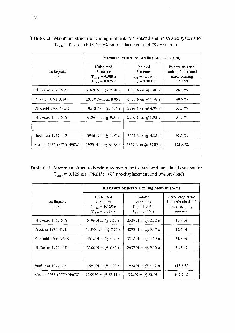
172
Table C.3 Maximum structure bending moments for isolated and unisolated systems for T1unis = 0.5 sec (PRSIS: 0% pre-displacement and 0% pre-load)
Maximum Structure Bending Moment (N-m)
Unisolated Isolated Percentage ratio: Earthquake Structure Structure isolated/unisolated
Input T lunis = 0.500 S Tlis = 1.116 S max. bending T2unis = 0.076 S T2;, = 0.083 S moment
El Centro 1940 N-S 6369 N-m @ 2.38 s 1665 N-m @ 3.00 s 26.1%
Pacoima 1971 S16E 13550 N-m @ 8.86 s 6573 N-m @ 3.58 s 48.5%
Parkfield 1966 N65E 10510 N-m@ 4.34 s 3394 N-m @ 4.99 s 32.3%
El Centro 1979 N-S 6136 N-m @ 9.04 s 2090 N-m@ 9.92 s 34.1%
Bucharest 1977 N-S 3946 N-m @ 3.97 s 3657 N-m @ 4.28 s 92.7%
Mexico 1985 (SCT) N90W 1929 N-m @ 64.88 s 2349 N-m @ 58.02 s 121.8%
Table C.4 Maximum structure bending moments for isolated and unisolated systems for T1unis = 0.125 sec (PRSIS: 16% pre-displacement and 0% pre-load)
Maximum Structure Bending Moment (N-m)
Unisolated Isolated Percentage ratio: Earthquake Structure Structure isolated/unisolated
Input Tlunis = 0.125 S Tlis = 1.006 S max. bending T2unis = 0.019 S T2;, = 0.022 S moment
El Centro 1940 N-S 5406 N-m @ 2.61 s 2526 N-m @ 2.22 s 46.7%
Pacoima 1971 S 16E 15530 N-m @ 7.75 s 4293 N-m @ 3.47 s 27.6%
Parkfield 1966 N65E 4612 N-m @ 4.21 s 3312 N-m @ 4.89 s 71.8%
El Centro 1979 N-S 3366 N-m @ 6.82 s 2037 N-m @ 9.10 s 60.5%
Bucharest 1977 N-S 1692 N-m@ 3.99 s 1920 N-m @ 4.02 s 113.5%
Mexico 1985 (SCT) N90W 1255 N-m @ 58.11 s 1354 N-m @ 58.98 s 107.9%
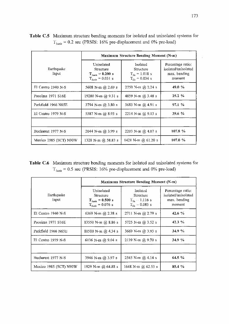
173
Table C.S Maximum structure bending moments for isolated and unisolated systems for
T1unis = 0.2 sec (PRSIS: 16% pre-displacement and 0% pre-load)
Maximum Structure Bending Moment (N-m)
Unisolated Isolated Percentage ratio: Earthquake Structure Structure isolated/unisolated
Input T lunis = 0.200 S Tlis = 1.018 S max. bending Tzunis = 0.031 S T2;, = 0.034 S moment
El Centro 1940 N-S 5608 N-m @ 2.69 s 2750 N-m @ 2.24 s 49.0%
Pacoima 1971 S16E 19280 N-m@ 9.31 s 4859 N-m @ 3.48 s 25.2%
Parkfield 1966 N65E 3794 N-m @ 3.80 s 3683 N-m @ 4.91 s 97.1%
El Centro 1979 N-S 5587 N-m @ 8.93 s 2214 N-m@ 9.13 s 39.6%
Bucharest 1977 N-S 2044 N-m@ 3.99 s 2203 N-m @ 4.07 s 107.8%
Mexico 1985 (SCT) N90W 1328 N-m@ 58.83 s 1421 N-m @ 61.20 s 107.0%
Table C.6 Maximum structure bending moments for isolated and unisolated systems for
T 1unis = 0.5 sec (PRSIS: 16% pre-displacement and 0% pre-load)
Maximum Structure Bending Moment (N-m)
Unisolated Isolated Percentage ratio: Earthquake Structure Structure isolated!unisolated
Input T lunis = 0.500 S Tlis = 1.116 S max. bending Tzunis = 0.076 S T2;, = 0.083 S moment
El Centro 1940 N-S 6369 N-m @ 2.38 s 2711 N-m @ 2.79 s 42.6%
Pacoima 1971 S 16E 13550 N-m @ 8.86 s 5725 N-m @ 3.52 s 42.3%
Parkfield 1966 N65E 10510 N-m @ 4.34 s 3669 N-m@ 3.93 s 34.9%
El Centro 1979 N-S 6136 N-m @ 9.04 s 2139 N-m @ 9.70 s 34.9%
Bucharest 1977 N-S 3946 N-m @ 3.97 s 2545 N-m@ 4.14 s 64.5%
Mexico 1985 (SCT) N90W 1929 N-m @ 64.88 s 1648 N-m @ 62.53 s 85.4%
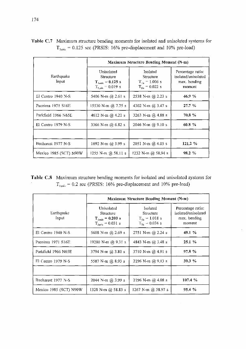
174
Table C. 7 Maximum structure bending moments for isolated and unisolated systems for T1unis = 0.125 sec (PRSIS: 16% pre-displacement and 10% pre-load)
Maximum Structure Bending Moment (N-m)
Unisolated Isolated Percentage ratio: Earthquake Structure Structure isolated/unisolated
Input Tlunis = 0.125 S T1;, = 1.006 S max. bending Tzunis = 0.019 S T2;, = 0.022 S moment
El Centro 1940 N-S 5406 N-m @ 2.61 s 2538 N-m@ 2.23 s 46.9%
Pacoima 1971 S16E 15530 N-m@ 7.75 s 4302 N-m @ 3.47 s 27.7%
Parkfield 1966 N65E 4612 N-m@ 4.21 s 3263 N-m @ 4.88 s 70.8%
E1 Centro 1979 N-S 3366 N-m @ 6.82 s 2046 N-m@ 9.10 s 60.8%
Bucharest 1977 N-S 1692 N-m @ 3.99 s 2051 N-m@ 4.05 s 121.2%
Mexico 1985 (SCT) N90W 1255 N-m @ 58.11 s 1232 N-m @ 58.94 s 98.2%
Table C.8 Maximum structure bending moments for isolated and unisolated systems for T1unis = 0.2 sec (PRSIS: 16% pre-displacement and 10% pre-load)
Maximum Structure Bending Moment (N-m)
Unisolated Isolated Percentage ratio: Earthquake Structure Structure isolated/unisolated
Input T Innis = 0.200 S Tlis = 1.018 S max. bending Tzunis = 0.031 S T2is = 0.034 S moment
El Centro 1940 N-S 5608 N-m @ 2.69 s 2751 N-m@ 2.24 s 49.1%
Pacoima 1971 S16E 19280 N-m@ 9.31 s 4843 N-m @ 3.48 s 25.1%
Parkfield 1966 N65E 3794 N-m @ 3.80 s 3710 N-m @ 4.91 s 97.8%
El Centro 1979 N-S 5587 N-m @ 8.93 s 2196 N-m @ 9.13 s 39.3%
Bucharest 1977 N-S 2044 N-m@ 3.99 s 2196 N-m@ 4.08 s 107.4%
Mexico 1985 (SCT) N90W 1328 N-m @ 58.83 s 1267 N-m @ 58.97 s 95.4%
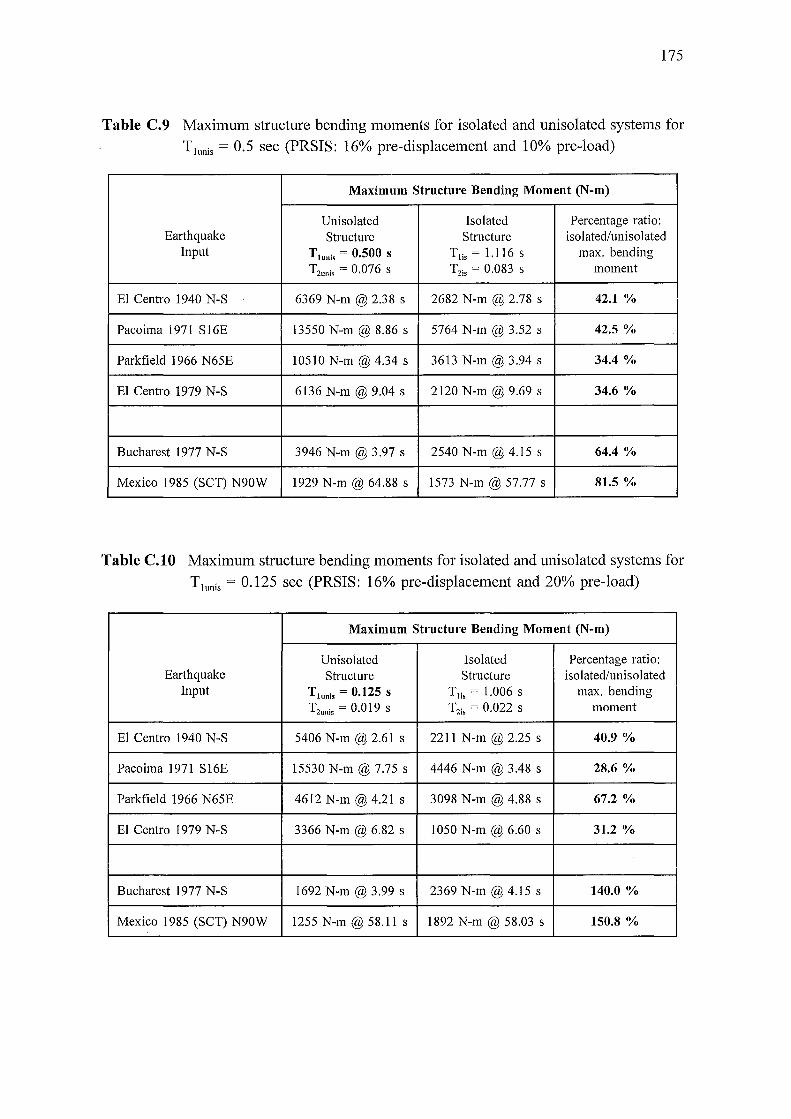
175
Table C.9 Maximum structure bending moments for isolated and unisolated systems for T1unis = 0.5 sec (PRSIS: 16% pre-displacement and 10% pre-load)
Maximum Structure Bending Moment (N-m)
Unisolated Isolated Percentage ratio: Earthquake Structure Structure isolated/unisolated
Input Tlunis = 0.500 S Tlis = 1.116 S max. bending T2unis = 0.076 S T2is = 0.083 S moment
El Centro 1940 N-S 6369 N-m @ 2.38 s 2682 N-m @ 2.78 s 42.1%
Pacoima 1971 S16E 13550 N-m @ 8.86 s 5764 N-m @ 3.52 s 42.5%
Parkfield 1966 N65E 10510 N-m @ 4.34 s 3613 N-m@ 3.94 s 34.4%
El Centro 1979 N-S 6136 N-m @ 9.04 s 2120 N-m@ 9.69 s 34.6%
Bucharest 1977 N-S 3946 N-m @ 3.97 s 2540 N-m @ 4.15 s 64.4%
Mexico 1985 (SCT) N90W 1929 N-m@ 64.88 s 1573 N-m @ 57.77 s 81.5%
Table C.lO Maximum structure bending moments for isolated and unisolated systems for T1unis = 0.125 sec (PRSIS: 16% pre-displacement and 20% pre-load)
Maximum Structure Bending Moment (N-m)
Unisolated Isolated Percentage ratio: Earthquake Structure Structure isolated/unisolated
Input Tlunis = 0.125 S Tn, = 1.006 s max. bending T2unis = 0.019 S T2is = 0.022 S moment
El Centro 1940 N-S 5406 N-m@ 2.61 s 2211 N-m @ 2.25 s 40.9%
Pacoima 1971 S16E 15530 N-m @ 7.75 s 4446 N-m @ 3.48 s 28.6%
Parkfield 1966 N65E 4612 N-m@ 4.21 s 3098 N-m @ 4.88 s 67.2%
El Centro 1979 N-S 3366 N-m @ 6.82 s 1050 N-m @ 6.60 s 31.2%
Bucharest 1977 N-S 1692 N-m @ 3.99 s 2369 N-m@ 4.15 s 140.0%
Mexico 1985 (SCT) N90W 1255 N-m@ 58.11 s 1892 N-m@ 58.03 s 150.8%
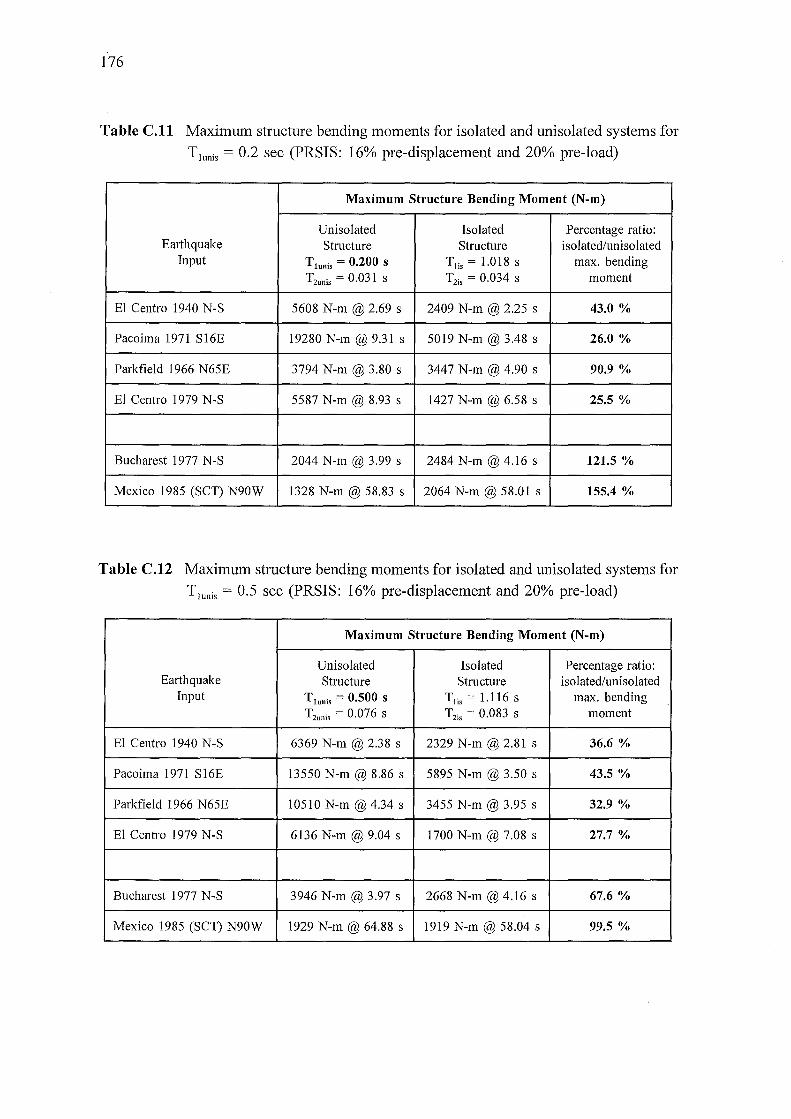
176
Table C.ll Maximum structure bending moments for isolated and unisolated systems for T1unis = 0.2 sec (PRSIS: 16% pre-displacement and 20% pre-load)
Maximum Structure Bending Moment (N-m)
Unisolated Isolated Percentage ratio: Earthquake Structure Structure isolated/unisolated
Input T lunis = 0.200 S Tlis = 1.018 S max. bending Tzunis = 0.031 S Tzis = 0.034 S moment
El Centro 1940 N-S 5608 N-m @ 2.69 s 2409 N-m @ 2.25 s 43.0%
Pacoima 1971 S16E 19280 N-m@ 9.31 s 5019 N-m @ 3.48 s 26.0%
Parkfield 1966 N65E 3794 N-m@ 3.80 s 3447 N-m@ 4.90 s 90.9%
El Centro 1979 N-S 5587 N-m @ 8.93 s 1427 N-m @ 6.58 s 25.5%
Bucharest 1977 N-S 2044 N-m@ 3.99 s 2484 N-m@ 4.16 s 121.5 %
Mexico 1985 (SCT) N90W 1328 N-m @ 58.83 s 2064 N-m @ 58.01 s 155.4%
Table C.12 Maximum structure bending moments for isolated and unisolated systems for
T1unis = 0.5 sec (PRSIS: 16% pre-displacement and 20% pre-load)
Maximum Structure Bending Moment (N-m)
Unisolated Isolated Percentage ratio: Earthquake Structure Structure isolated/unisolated
Input T lunis = 0.500 S Tlis = 1.116 S max. bending Tzunis = 0.076 S Tzis = 0.083 S moment
El Centro 1940 N-S 6369 N-m@ 2.38 s 2329 N-m @ 2.81 s 36.6%
Pacoima 1971 S 16E 13550 N-m @ 8.86 s 5895 N-m @ 3.50 s 43.5%
Parkfield 1966 N65E 10510 N-m@ 4.34 s 3455 N-m @ 3.95 s 32.9%
El Centro 1979 N-S 6136 N-m @ 9.04 s 1700 N-m @ 7.08 s 27.7%
Bucharest 1977 N-S 3946 N-m@ 3.97 s 2668 N-m @ 4.16 s 67.6%
Mexico 1985 (SCT) N90W 1929 N-m@ 64.88 s 1919 N-m @ 58.04 s 99.5%
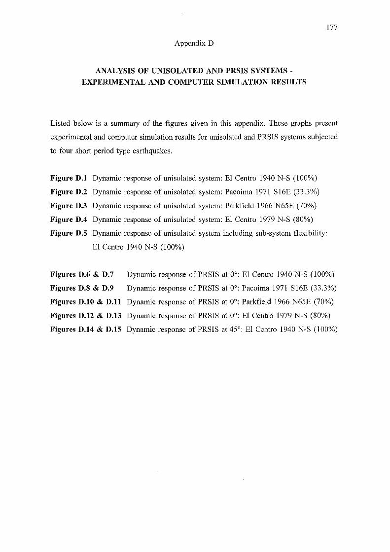
Appendix D
ANALYSIS OF UNISOLATED AND PRSIS SYSTEMS -
EXPERIMENTAL AND COMPUTER SIMULATION RESULTS
177
Listed below is a summary of the figures given in this appendix. These graphs present
experimental and computer simulation results for unisolated and PRSIS systems subjected
to four short period type earthquakes.
Figure D.l Dynamic response of unisolated system: El Centro 1940 N-S (100%)
Figure D.2 Dynamic response of unisolated system: Pacoima 1971 S16E (33.3%)
Figure D.3 Dynamic response of unisolated system: Parkfield 1966 N65E (70%)
Figure D.4 Dynamic response of unisolated system: El Centro 1979 N-S (80%)
Figure D.5 Dynamic response of unisolated system including sub-system flexibility:
El Centro 1940 N-S (100%)
Figures D.6 & D.7 Dynamic response of PRSIS at 0°: El Centro 1940 N-S (100%)
Figures D.8 & D.9 Dynamic response of PRSIS at 0°: Pacoima 1971 S16E (33.3%)
Figures D.lO & D.ll Dynamic response of PRSIS at 0°: Parkfield 1966 N65E (70%)
Figures D.12 & D.13 Dynamic response of PRSIS at 0°: El Centro 1979 N-S (80%)
Figures D.14 & D.15 Dynamic response of PRSIS at 45°: El Centro 1940 N-S (100%)
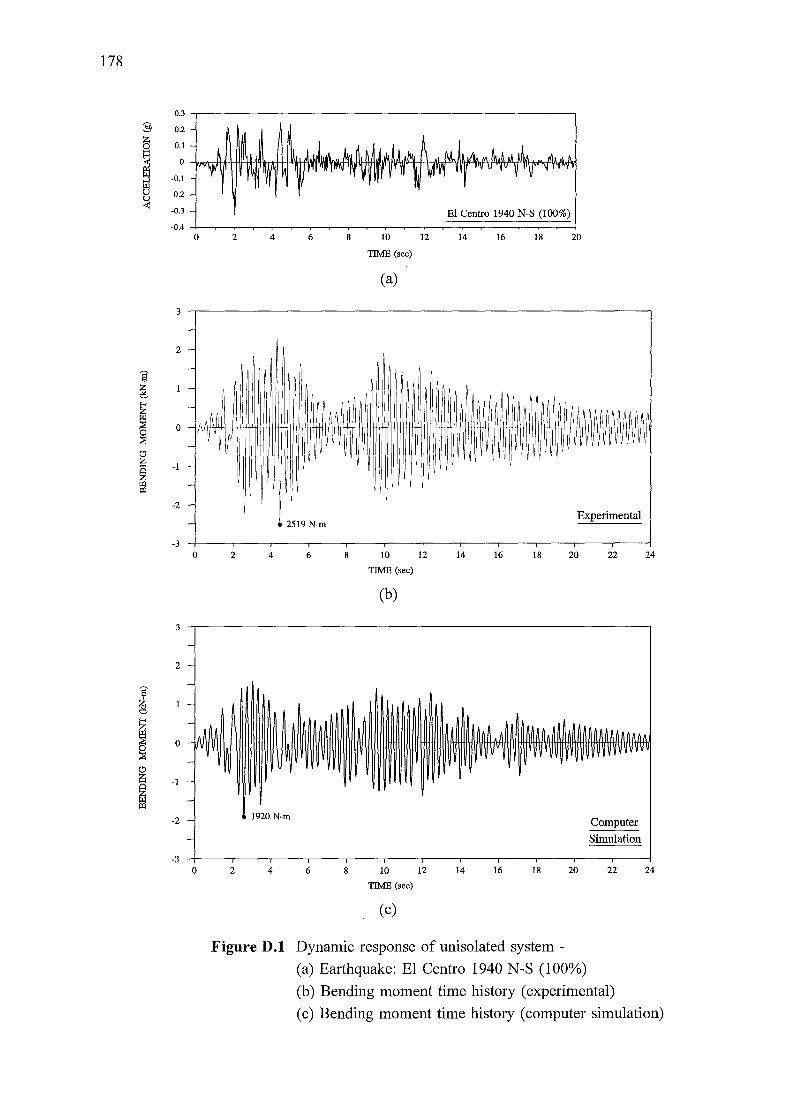
178
:§
5
~ t:l ~
s ~ ~ ~ ~ ~ ffi "'
0.3
0.2
0.1
0
-0.1
-0.2
-0.3
-0.4 0 2 4 6
3
-2 - l
--
0
-I ~~I .!\~~
Tlilfl II~~ -
-1 -- I
-2 -- 2519 N-m
-3 0 2 4 6
8
8
10
TIME (sec)
(a)
10
TIME (sec)
(b)
12
12
El Centro 1940 N-S (100%)
14 16 18 20
.~ \II~~~~~~A~W v vrmm~m
Experimental
14 16 18 20 22 24
3 ~----------------------------------------------------~
2
0
-1
-2
0
1920N-m
2 4 6 10 12
TIME (sec)
(c)
14 16 18 20
Computer
Simulation
22 24
Figure D.l Dynamic response of unisolated system-
(a) Earthquake: El Centro 1940 N-S (100%)
(b) Bending moment time history (experimental)
(c) Bending moment time history (computer simulation)

179
0.3
:§ 0.2
5 0.1
~ 0
-0.1
~ -0.2
-0.3 Pacoima 1971 Sl6E (33.3%) -0.4
0 2 4 6 8 10 12 14 16 18 20
TIME (sec)
(a)
3
2491 N-m
2
I ~ ~ g
~ 0 WMN ~
I -1
-2 Experimental
-3 0 2 4 6 8 10 12 14 16 18 20 22 24
TIME (sec)
(b)
3
2
~ g
~ 0
~
I -1
IX!
-2 1889 N-m Computer
Simulation
-3 0 2 4 6 8 10 12 14 16 18 20 22 24
TIME (sec)
(c)
Figure D.2 Dynamic response of unisolated system -
(a) Earthquake: Pacoima 1971 S16E (33.3%)
(b) Bending moment time history (experimental)
(c) Bending moment time history (computer simulation)
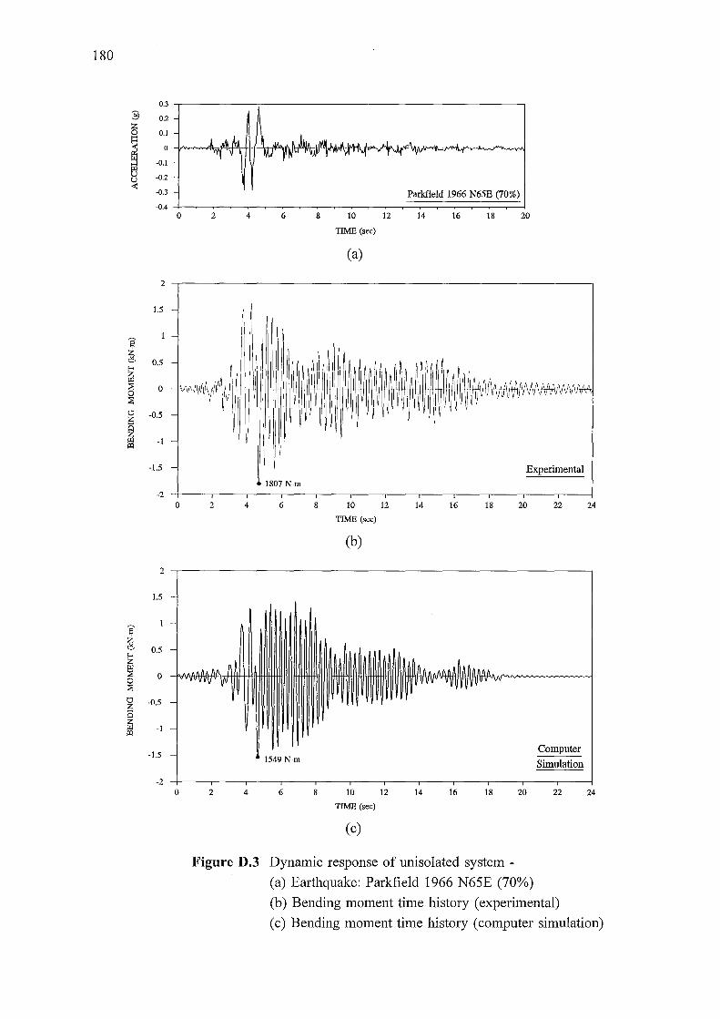
180
0.3
3 0.2
6 0.1
~ 0
-0.1
B -0.2 u < -0.3 Parkfield 1966 N65E (70%)
-0.4 0 2 4 6 8 10 12 14 16 18 20
TIME (sec)
(a)
2
1.5 -
-~ g
0.5 -
I 0
" -0.5 ~
_,~A.Iii~ I~ I~AAA AAAAA AA AAA
ryr ~V !~ ~~~VI) VVVVVVV VV VVVV •v '"
-
ffi -1 ... -
-1.5 - Experimental 1807 N-m
-2 0 2 4 6 8 10 12 14 16 18 20 22 24
TIME (sec)
(b)
2
1.5
s: ~ 0.5
~ 0
~ ~ -0.5
~ -1
-1.5 Computer
1549 N-m Simulation
-2 0 2 4 6 10 12 14 16 18 20 22 24
TIME (sec)
(c)
Figure D.3 Dynamic response of unisolated system -
(a) Earthquake: Parkfield 1966 N65E (70%)
(b) Bending moment time history (experimental)
(c) Bending moment time history (computer simulation)
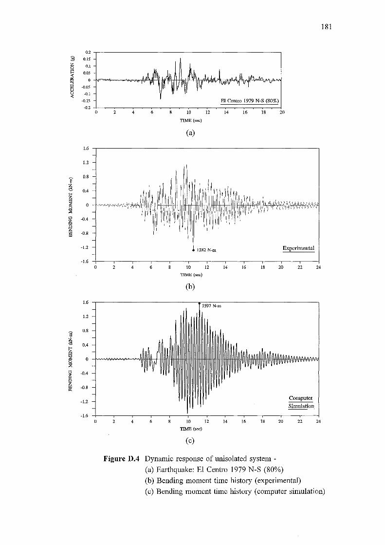
181
0.2
:§ 0.15
~ 0.1
~ 0.05
0
tS -0.05
~ -0.1
-0.15 El Centro 1979 N-S (80%) -0.2
0 2 4 6 8 10 12 14 16 18 20
TIME (sec)
(a)
1.6
1.2
s 0.8
~ 0.4
~ 0
~
I -0.4
-0.8
-1.2 1282 N-m Experimental
-1.6 0 2 4 6 8 10 12 14 16 18 20 22 24
TIME (sec)
(b)
1.6 1597 N-m
1.2
s 0.8
~ 0.4
~ 0
~ ~ -0.4
~ -0.8
-1.2 Computer
Simulation
-1.6 0 2 4 6 8 10 12 14 16 18 20 22 24
TIME (sec)
(c)
Figure D.4 Dynamic response of unisolated system -
(a) Earthquake: El Centro 1979 N-S (80%)
(b) Bending moment time history (experimental)
(c) Bending moment time history (computer simulation)
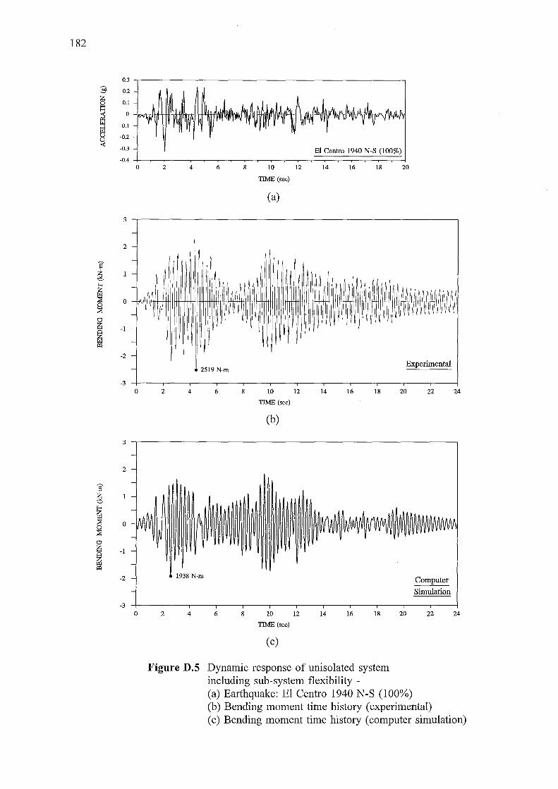
182
0.3
3 0.2 z
0.1 0
i 0
-0.1
u -0.2 u ~
-0.3
-0.4 0 2 4
3
-
2 -
-
-
- AA~ r ~
0
-
-1 --
-2 -
-
-3 0 2 4
3
2
~ g
~ 0 ~
I -1
>Q
-2
-3 0 2 4
Figure D.S
6 8 10
TIME (sec)
(a)
12
El Centro 1940 N-S (100%)
14 16 18 20
l1ill !
::8 I~
2519 N-m Experimental
6 8 10 12 14 16 18 20 22 24
TIME (sec)
(b)
Computer
Simulation
6 10 12 14 16 18 20 22 24
TIME (sec)
(c)
Dynamic response of unisolated system including sub-system flexibility -(a) Earthquake: El Centro 1940 N-S (100%) (b) Bending moment time history (experimental) (c) Bending moment time history (computer simulation)
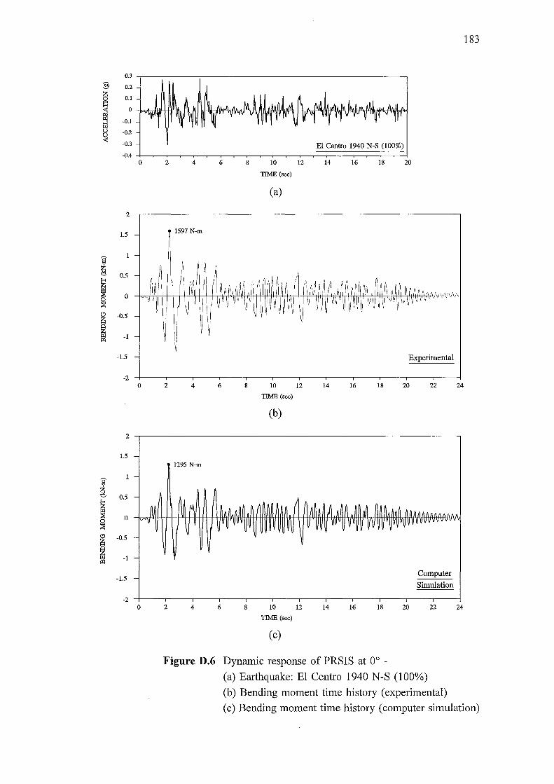
0.3 ..----------,----------------------,
0.2
0.1
0 ~~~~~~~~11H~:i~~mP~Hhl.I~W~~~~dJ~fW~~~~~~f~~~~~W~
-0.1
-0.2
-0.3 El Centro 1940 N-S (100%) -0.4 -~-~~--,-~~~~--,-~~-.-~~==;::::::::::;::=::::;::::::;::::=;:=;::::::__j
0 2 4 6 8 10
TIME (sec)
(a)
12 14 16 18 20
2 ,------------------------------.
1.5 1597 N-m
0.5
0
-0.5
-1
-1.5 Experimental
-2 ~--.--.---.--.--.---.--.---.--,.--,---.-~ 0 2 4 6 8 10 12 14 16 18 20 22 24
TIME (sec)
(b)
2 .------------------------------.
1.5
0.5
0
-0.5
-1
-1.5
1295 N-m
Computer
Simulation
~ ~--.--.---.--.--.---.--.---.--.--,---.-~
0 2 4 6 8 10 12 14 16 18 20 22 24
TIME (sec)
(c)
Figure D.6 Dynamic response of PRSIS at oo -(a) Earthquake: El Centro 1940 N-S (100%)
(b) Bending moment time history (experimental)
183
(c) Bending moment time history (computer simulation)
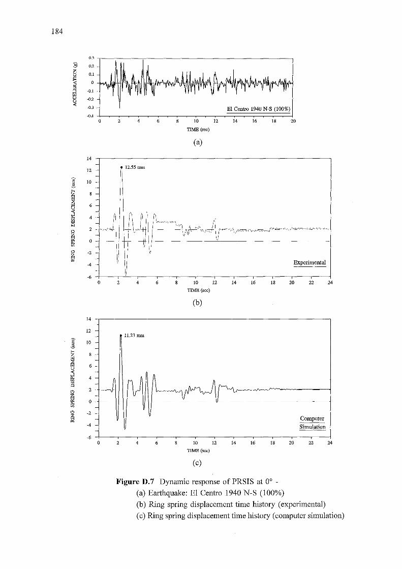
184
0.3
§ 0.2 z
0.1
I 0
-0.1
u -{).2
~ -0.3
-{).4
0
14 -
12 --
1 10 --
~ 8
6
4 "' s C!l 2
----
=~} ~ 0
-
"' -C!l -2
~ --
-4 --
-6 0
14
12
1 10
~ 8
~ 6 u
~ 4 ~ 0 C!l 2
~ 0
"' C!l -2
~ -4
-6 0
2 4
12.55mm
(\ f v
2 4
2 4
6 8 10
TIME (sec)
(a)
12
El Centro 1940 N-S (100%)
14 16 18 20
\"""1 IV f-----~· "~ ~··yMO fV·'Y"""'~· . ['- /"''~"''t-J'"'Ij>-,f\--1\rA'Vv\r,
·--·--·----------··~
Experimental
6 8 10 12 14 16 18 20 22 24
TIME (sec)
(b)
·-------
Computer
Simulation
6 10 12 14 16 18 20 22 24
TIME (sec)
(c)
Figure D.7 Dynamic response of PRSIS at oo -(a) Earthquake: El Centro 1940 N-S (100%)
(b) Ring spring displacement time history (experimental)
(c) Ring spring displacement time history (computer simulation)
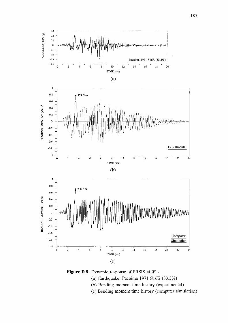
0.3
:§ 0.2 z 0 0.1
~ 0
-0.1 e)
-0.2 u ...: -0.3
-0.4
0.8
0.6
1 ~
0.4
; 0.2
0
~ -0.2
I -0.4
-0.6
-0.8
-1
0.8
0.6
1 ~
0.4
; 0.2
0
~
I -0.2
-0.4
-0.6
-0.8
-1
0 2 4 6
779 N-m
,;,"i· I~
0 2 4 6
708 N-m
0 2 4 6
8
8
8
10
TIME (sec)
(a)
12
....
10 12
TIME (sec)
(b)
10 12
TIME (sec)
(c)
~~ I~ I
Pacoima 1971 S16E (33.3%)
14 16
II l\1
14 16
14 16
18 20
I~~~ A !\j\fA (\I) A A" "'II" '1/11\1 ~~~~~~ 11VVV\fvvwvv
18
18
Experimental
20
20
22
Computer
Simulation
22
24
24
185
Figure D.8 Dynamic response of PRSIS at oo -(a) Earthquake: Pacoima 1971 S16E (33.3%)
(b) Bending moment time history (experimental)
(c) Bending moment time history (computer simulation)
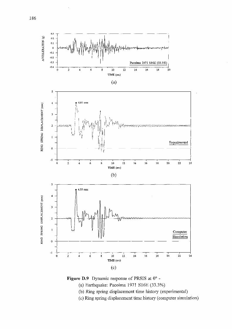
186
0.3
:§ 0.2
6 0.1
! 0
-0.1
u -0.2 ~
-0.3 Pacoima 1971 S16E (33.3%) -0.4
0 2 4 6 8 10 12 14 16 18 20
TIME (sec)
(a)
5
I 4
~
~ 3
u
~ s 2
d
~ "' Experimental d
~ 0
-1 0 2 4 6 8 10 12 14 16 18 20 22 24
TIME (sec)
(b)
5
I 4
I 3
u
~ s 2
d
~ Computer
"' Simulation d
~ 0
-1 0 2 4 6 8 10 12 14 16 18 20 22 24
TIME (sec)
(c)
Figure D.9 Dynamic response of PRSIS at oo -(a) Earthquake: Pacoima 1971 S16E (33.3%)
(b) Ring spring displacement time history (experimental)
(c) Ring spring displacement time history (computer simulation)
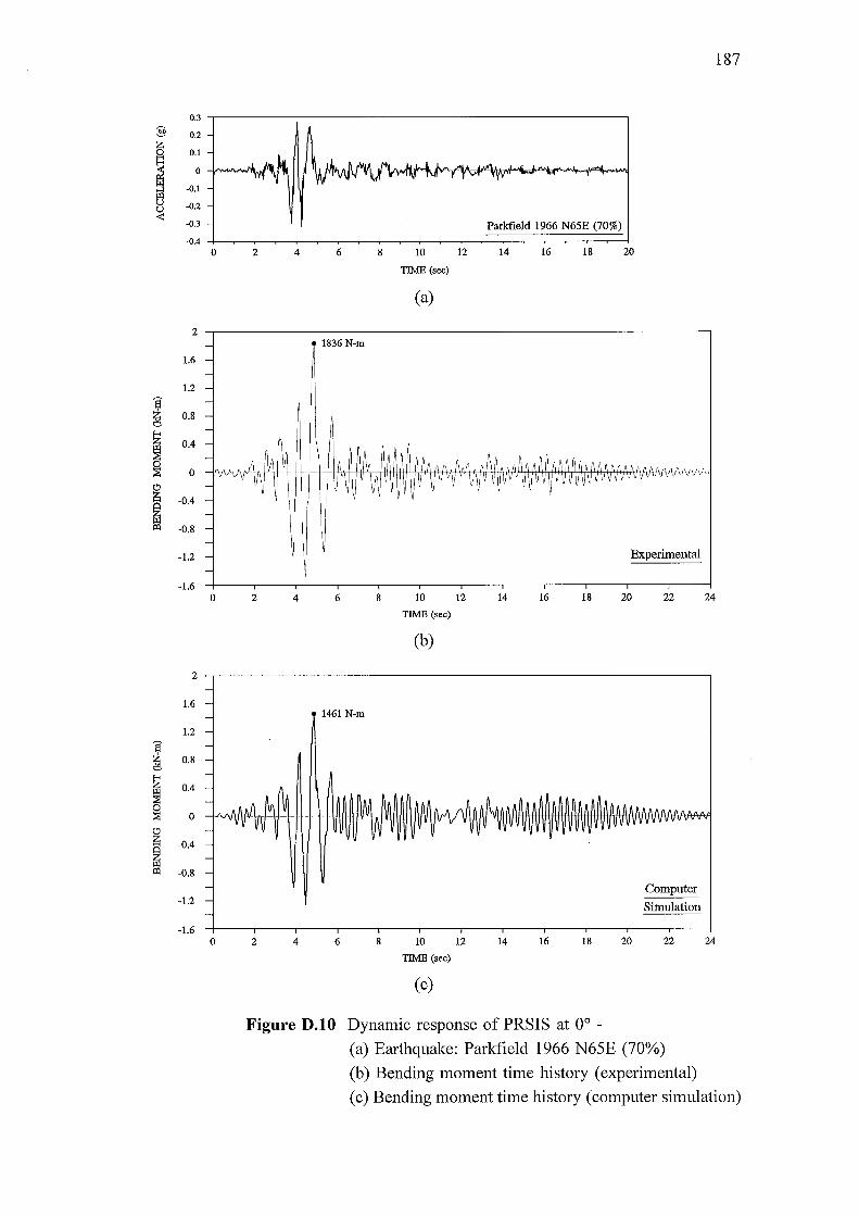
187
0.3
:§ 0.2 z 0 0.1
~ 0
-0.1
El -0.2 u ...: -0.3 Parkfield 1966 N65E (70%) -0.4
0 2 4 6 8 10 12 14 16 18 20
TIME (sec)
(a)
2 1836 N-m
1.6
1.2
s ~ 0.8
! 0.4
0 ~A A~~A6~~AAA~b~AAtv N flfAAAtt/V+t
I 'V ~v V ~v V V V vvv \/Vifif'r \ 1
\. ·
-0.4
-0.8
-1.2 Experimental
-1.6 0 2 4 6 8 10 12 14 16 18 20 22 24
TIME (sec)
(b)
2
1.6 1461 N-m
1.2
1 ~ 0.8
~ 0.4
~ 0
C!l ~ -0.4
ffi ~ -0.8
Computer -1.2
Simulation
-1.6 0 2 4 6 8 10 12 14 16 18 20 22 24
TIME (sec)
(c)
Figure D.lO Dynamic response of PRSIS at oo -(a) Earthquake: Parkfield 1966 N65E (70%)
(b) Bending moment time history (experimental)
(c) Bending moment time history (computer simulation)

188
0.3
:§ 0.2 z 0 0.1
~ 0
~ -0.1
u -0.2 u ..:: -0.3
-0.4
16
14
I 12
10 rz;
~ 8
u 6
~ 4 s 2
~ 0
"' -2 (.?
~ -4
-6
-8
16
14
I 12
10 E-<
~ 8
6
~ 4 s 2
~ 0
"' -2 (.?
~ -4
-6
-8
0 2 4 6 8
- 14.29 mm
-
-
-
-
-r~"~'\f·~Av ·v
10
TIME (sec)
(a)
12
Parkfield 1966 N65E (70%)
14 16 18 20
-~-~~- --
---··-
-
-
-
0 2 4 6 8 10 12 14 16 18
TIME (sec)
(b)
-13.27 nun
-
-
-
-
-~ n
·v
-f--------- ..
-
-
-
0 2 4 6 8 10 12 14 16 18
TIME (sec)
(c)
Figure D.ll Dynamic response of PRSIS at oo -(a) Earthquake: Parkfield 1966 N65E (70%)
Experimental
20 22
Computer
Simulation
20 22
(b) Ring spring displacement time history (experimental)
24
24
(c) Ring spring displacement time history (computer simulation)
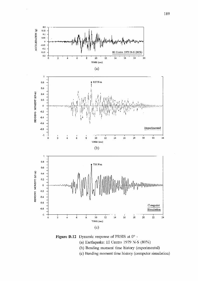
0.2
§ 0.15
~ 0.1
~ 0.05
0
!:J -0.05
u -0.1 < -0.15
-0.2 0
0.8
0.6
1 0.4
~
~ 0.2
0
~ Cl -0.2
I -0.4
~ -0.6
-0.8
-1 0
0.8
0.6
s ~
0.4
~ 0.2
0
~
I -0.2
-0.4
-0.6
-0.8
-1 0
2 4 6 8
2 4 6 8
2 4 6 8
10
TIME (sec)
(a)
819 N-m
r l i
10
TIME (sec)
(b)
718 N-m
10
TIME (sec)
(c)
El Centro 1979 N-S (80%)
12 14 16 18
12 14 16 18
12 14 16 18
20
·WWww
Experimental
20
20
22
Computer
Simulation
22
24
24
189
Figure D.12 Dynamic response of PRSIS at oo -(a) Earthquake: El Centro 1979 N-S (80%)
(b) Bending moment time history (experimental)
(c) Bending moment time history (computer simulation)
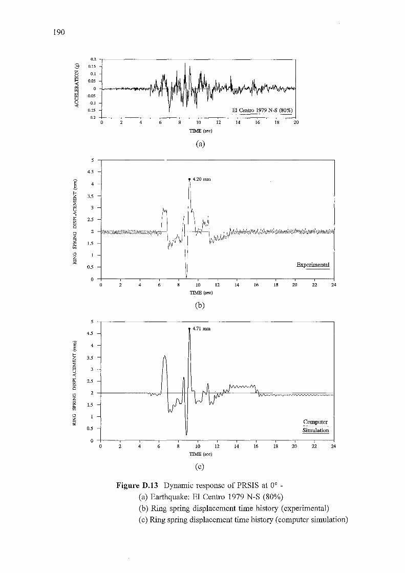
190
0.2 -,-------------------------------,
0.15
0.1
0.05
0 ~_,._,.......,_.....,l'\'l"i''>"'\JI'I'df-'l-lliHft--t't.f-IL•I-i~ttHY'/III./\I"W'l,,--A-,f-W"\illhr'lfll-IJ'4r
-0.05
-0.1
-0.15 El Centro 1979 N-S (80%) -0.2 -!-~~~-~~~~~-~~-.-~~~;::::::;:=~=;==::;::~~
0 2 4 6 8 10
TIME (sec)
(a)
12 14 16 18 20
5 .----------------------------~
4.5 -
4.20mm 4 -
3.5 -
d 1 -
~ 0.5 - Experimental
0 2 4 6 8 10 12 14 16 18 20 22 24
TIME (sec)
(b)
5 .----------------------------~
4.71 mm
Computer
Simulation
0 ~--.--.---,--,,---,---.--.---,--.--.---.-~ 0 2 4 6 8 10 12 14 16 18
TIME (sec)
(c)
Figure D.l3 Dynamic response of PRSIS at oo -(a) Earthquake: El Centro 1979 N-S (80%)
20 22
(b) Ring spring displacement time history (experimental)
24
(c) Ring spring displacement time history (computer simulation)
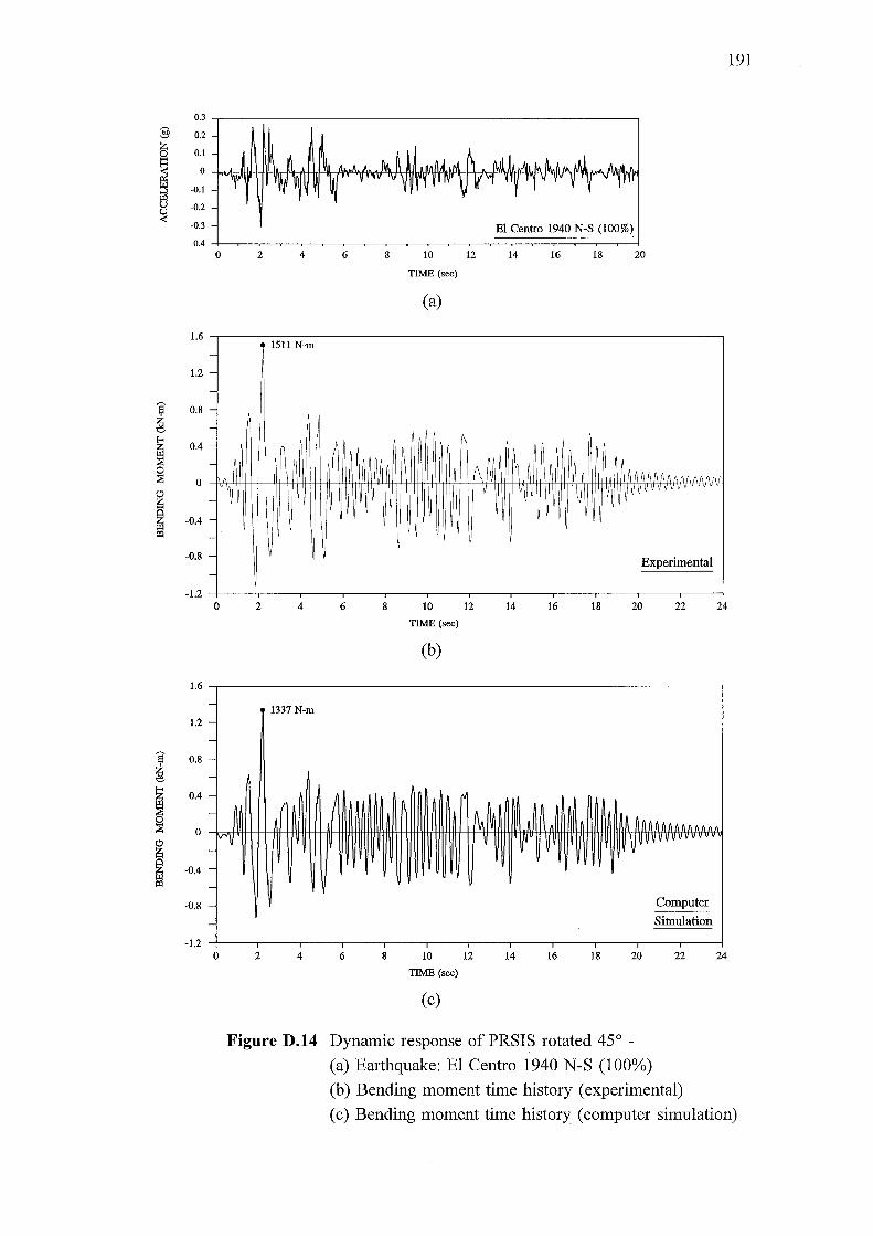
0.3
§ 0.2
~ 0.1
~ 0
-0.1
t3 -0.2
~ -0.3
-0.4
1.6
1.2
s.: 0.8
g
~ 0.4
~ 0
~ ffi -0.4 ill
-0.8
-1.2
1.6
1.2
s ~
0.8
~ 0.4
~ 0
I -0.4
-0.8
-1.2
0 2 4
1511 N-m -----
-~
-~
- \~ --
-
-
0 2 4
- 1337 N-m -----
- N I'
IV"V -----
0 2 4
6 8
~I
6 8
l I~
6 8
10
TIME (sec)
(a)
10
TIME (sec)
(b)
10
TIME (sec)
(c)
El Centro 1940 N-S (100%)
12 14 16 18 20
(\
t\N 1'1. ~. 1\li ~AAAAAI\A V\M v v~ ~ \J ~\, ~ V v v v v v v 1\Mr
Experimental
12 14 16 18 20 22 24
~~ ~.AI i\ nl ~AAAAAAAAAnn ~ ~v· vv IVVVVVVV •v
Computer
Simulation
12 14 16 18 20 22 24
Figure D.14 Dynamic response of PRSIS rotated 45° -
(a) Earthquake: El Centro 1940 N-S (100%)
(b) Bending moment time history (experimental)
191
(c) Bending moment time history (computer simulation)
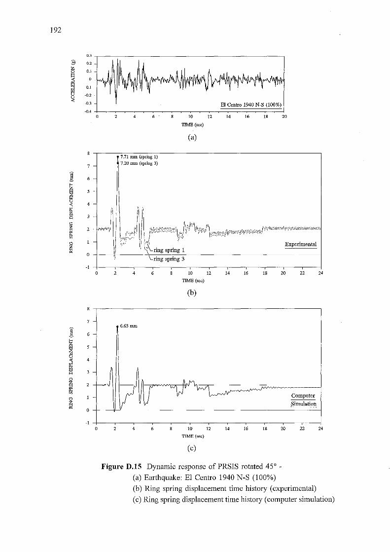
192
0.3
:§ 0.2
~ 0.1
~ 0
-0.1 ~ u -0.2 u ...:
-0.3 El Centro 1940 N-S (100%) -0.4
0 2 4 6 . 8 10 12 14 16 18 20
TIME (sec)
(a)
7.71 mm (spring 1)
7 7.20 mm (spring 3)
j 6 E-<
~ 5
~ 4
s 3
0
~ 2
"' 0
v 0- ring spring 1 Experimental
~ 0
. \.:ring spring 3
-1 0 2 4 6 8 10 12 14 16 18 20 22 24
TIME (sec)
(b)
8
7
j 6
I 5
~ 4
s 3
0
~ 2
"' Computer 0
~ Simulation 0
-1 0 2 4 6 8 10 12 14 16 18 20 22 24
TIME (sec)
(c)
Figure D.lS Dynamic response of PRSIS rotated 45° -
(a) Earthquake: El Centro 1940 N-S (100%)
(b) Ring spring displacement time history (experimental)
(c) Ring spring displacement time history (computer simulation)


![SEISMIC ROOF ISOLATION OF HALKAPINAR … · most efficient seismic isolation solution for the Halkapınar Gymnasium. In this thesis, theory of seismic isolation, ... [18] (From AASHTO](https://img.pdfslide.us/doc/110x75/5b5ba6ce7f8b9a905c8e7903/seismic-roof-isolation-of-halkapinar-most-efficient-seismic-isolation-solution.jpg)