The Use of Sodium Polyacrylate to Increase Crop Production

in Dry-Land Farming

Kira E. Powell

Advanced Science Research, Odessa High School, Odessa, WA 99159

March 20, 2011

Abstract

Sodium polyacrylate (C3H3NaO2), originally developed by the Dow Chemical Company, is a

polymer that is a mix of sodium acrylate and acrylic acid. Commonly found in baby diapers,

it can absorb 500 times its mass in water. This polymer has potential as a soil additive. The

hypothesis was if sodium polyacrylate was applied to farmable soil then the yield in the

experimental section would be higher than the control section. This should be reflected by an

increase in wheat crop growth and water retention. Three plots were planted for the full scale

test, the Control Plot, the Experimental Plot 1 with a 2.5 % sodium polyacrylate mixture and

the Experimental Plot 2 with a 5.0 % sodium polyacrylate mixture. Multiple data collections

took place throughout the test including plant height, plant count, water present and yield.

The Control Plot resulted in 26.8 bushels per acre, the Experimental Plot 1 with 32.8 bushels

per acre and the Experimental Plot 2 with 34.1 bushels per acre. The hypothesis was

accepted because both Experimental Plots had a statistically higher average plant height and

yield then the Control Plot.

Introduction

Agriculture has been the foundation of civilization since it allowed the first people

to permanently settle in Mesopotamia over six thousand years ago; today it is no

different. Ninety-nine percent of all of food consumed by humans comes from cropland

(Lang, 2006). But many factors contribute to the success or failure of agricultural

production including drought, erosion, and average annual rainfall.

Today, the United States is experiencing severe cases of drought across the

country. Eighteen out of 50 states including North and South Carolina, Wisconsin and

Washington, have fallen victim to either hydrological droughts (drought due to deficiency

in precipitation affecting local surface or subsurface water supply) or agricultural

droughts (drought involving factors vital to agriculture production such as soil water

deficiency) (NDMC, 2006) (Figure 1). Although a natural phenomenon, droughts are

2

Figure 1. This chart shows how widespread

drought is in the United States as of February 1,

2011 (NDMC, 2011).

extremely costly, causing $6-$8 billion dollars loss annually for the United States (Hayes,

2004). And, unlike other natural disasters such as hurricanes and tornados, droughts have

more longstanding affects on a greater number of people. Several elements that

contribute to drought’s devastation, is the lack of predictability, the length (droughts can

last anywhere from several months to sixty years), and the wide scale of people it affects.

For example, the Dust Bowl during the 1930’s lasted eight years, affected 260 million

acres of cropland, and displaced nearly 2.5 million people (Monatana, 2009). A drought

can directly harm farmers and ranchers, with the loss of animals and crops. The ripple

consequences extending to the average person paying more for food. During the drought

in Australia in 2008 when thousands of acres of wheat was lost, prices rose from $258 to

$367 per ton in Australia and the global price of was inflated (Smith, 2008). It has been

theorized that the likelihood of disasters like this occurring could be reduced or entirely

eliminated with soil additives designed to absorb the moisture that is available. A

chemical that has such potential is sodium polyacrylate.

Sodium polyacrylate (C3H3NaO2)n, originally developed by the Dow Chemical

Company, is a polymer that is a mix of sodium polyacrylate and acrylic acid (Figure 2).

3

Commonly found in baby diapers and household cleaners, it can absorb 500 times its

mass in water and thus is classified as a hydrogel (France, 2008). A hydrogel is a

colloidal gel in which water is the dispersion medium. Sodium polyacrylate exists in

randomly coiled chains, and there is an absence of Na+ ions (salt is removed). The

negative charges on the coils repel each other causing them to unwind. Water is then

attracted to the negative ions and attached with hydrogen bonds. This phenomenon

allows 500 times the polymers weight in pure water to be absorbed, slightly less with

impure water (France, 2008). The polymer will continue to attach to water until all

negative ions are linked to water (Figure 3). These bonds are physical, not chemical,

allowing for the process to be reversed and then repeated indefinitely. Because of this

property sodium polyacrylate could be valuable soil additive.

A factor that has to be taken into consideration for every new soil additive, like

sodium polyacrylate, is cost effectiveness. Any treatment, no matter how beneficial, must

not compromise the profit of the crop. Ideally the benefit (additional profit) of the

Figure 2. Molecular structure of sodium

polyacrylate (Kelien, 2010).

Figure 3. A model of dry coiled sodium polyacrylate (left), and

an uncoiled strand bonded with water (Richer, 2007).

4

additive, whether it is a fertilizer or a pesticide, will outweigh the cost. For example, if an

additive cost $100 to seed an entire field then the additional yield resulting from its

application to the soil would need to equal or surpass the $100 in order to be considered

cost effective. In order for the sodium polyacrylate to be a viable soil additive it has to be

cost effective. Since the sodium polyacrylate would cost approximately $0.83-$1.65 to

seed one acre, the additional profit from the yield from that respective acre would have to

exceed that (ZGEPTC, 2011). The additional yield would result from the availability of

water that the chemical absorbed and the increased water potential.

Water potential is the possible amount of water a field can hold. This is also

called field capacity. This capacity changes with soil type. There are three main types:

sandy, loam and clay and they are named for the particle that is most present in its

composition. Sand particles are the largest followed by loam then clay. The size of the

resulting spaces between the particles, called capillaries, determines the suction force

exerted on water in the soil (Figure 4). Because the retention of water through suction is

less in sandy soils, sandy soils can not retain as much water resulting in a lower field

capacity. The opposite is true in clay soils. Clay is the finest of the three particles so

when soils are made up of mainly these particles, the resulting capillaries between the

particles are smaller. The smaller the capillaries, the more suction in them, thus clay soils

Figure 4. An illustration of the effect of

capillary size on suction (Boama, 2009).

5

can retain more water and have a higher field capacity. The downside to this is that water

is hard to extract from the clay soils. With sandy soils the water cannot be retained

adequately. The third type of soil is loamy or silty soil. Silt is the particle size between

clay and sand. It allows for big enough capillaries to easily release water but small

enough capillaries to provide adequate retention for growth. The relationship between

these soil types and their resulting field capacity can be seen in the water retention curve.

The soil type present at the Control and Experimental Plots was Shano Silt Loam. This

variety of soil has a high, 29.0 cm (11.4 in), available water capacity (NRCS, 2009). It

closely follows the loam line on the water retention curve (Figure 5).

The focus of this experiment was to test the effectiveness of sodium polyacrylate

as a soil additive in farmable soil to increase crop production. The hypothesis was if

sodium polyacrylate was applied to farmable soil then the yield in the experimental

section will be higher than the control section. This should be reflected by an increase in

wheat crop growth and water retention. Water retention in soil is directly linked to crop

Figure 5. The Soil water Retention Curve. The blue line, loam is

the closest to the Shono Loam Silt present in Plots (NIVAP, 2010).

6

Figure 6. The Pre-trial testing apparatus during a test

(Powell, 2010).

production, so theoretically, if water availability in farmable soil is increased for crops,

crop production should also be increased.

Materials and Methods

Pre-trials were done in the lab to determine the application method for the full

scale tests. Soil from the field that would later be used for the full scale test was collected

for laboratory tests. A small clear plastic tube was cut and wire mesh was hot glued to the

bottom of one end to prevent anything aside from water passing through. It was held

vertical, mesh down with a clamp and ring stand over a funneled graduated cylinder

(Figure 6). With this apparatus, tests were conducted to find how to position the sodium

polyacrylate in the soil (furrow or a broadcast method). The first test consisted of 100 g

of soil and 50 g of water in order to get a control without sodium polyacrylate. The test

lasted twenty four hours. The same procedure was repeated with 10 g sodium

polyacrylate to 90 g soil, (10 % sodium polyacrylate), 5 g sodium polyacrylate to 95 g

soil, (5 % sodium polyacrylate) and 1 g sodium polyacrylate to 99 g soil, (1 % sodium

polyacrylate). Each set was also tested using the two methods: 1) the polymer was mixed

into the soil, and 2) the polymer was set in as a layer at the bottom of apparatus. These

7

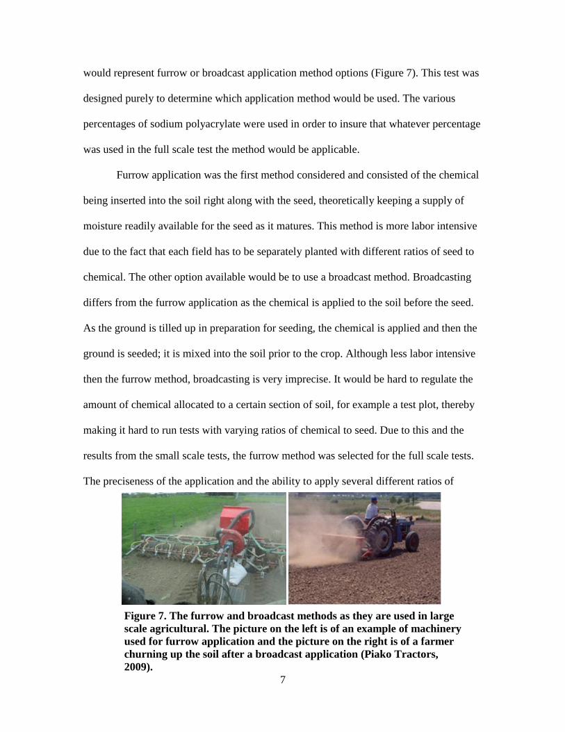
Figure 7. The furrow and broadcast methods as they are used in large

scale agricultural. The picture on the left is of an example of machinery

used for furrow application and the picture on the right is of a farmer

churning up the soil after a broadcast application (Piako Tractors,

2009).

would represent furrow or broadcast application method options (Figure 7). This test was

designed purely to determine which application method would be used. The various

percentages of sodium polyacrylate were used in order to insure that whatever percentage

was used in the full scale test the method would be applicable.

Furrow application was the first method considered and consisted of the chemical

being inserted into the soil right along with the seed, theoretically keeping a supply of

moisture readily available for the seed as it matures. This method is more labor intensive

due to the fact that each field has to be separately planted with different ratios of seed to

chemical. The other option available would be to use a broadcast method. Broadcasting

differs from the furrow application as the chemical is applied to the soil before the seed.

As the ground is tilled up in preparation for seeding, the chemical is applied and then the

ground is seeded; it is mixed into the soil prior to the crop. Although less labor intensive

then the furrow method, broadcasting is very imprecise. It would be hard to regulate the

amount of chemical allocated to a certain section of soil, for example a test plot, thereby

making it hard to run tests with varying ratios of chemical to seed. Due to this and the

results from the small scale tests, the furrow method was selected for the full scale tests.

The preciseness of the application and the ability to apply several different ratios of

8

chemical outweighed any disadvantages.

Sodium polyacrylate has never before been used in large scale agriculture and

because of this fact, application rates were unknown. Similar products were researched

and the application rates were based off their recommendations for their own products.

The most closely related product, ZEBA® made by Absorbent Technologies Inc., is a

starch based superabsorbent polymer that, like sodium polyacrylate absorbs

approximately 500 times its weight in water (Absorbent Technologies, 2009). The

company suggests using a 0.68 kg - 0.91 kg (1.5-2.0 lbs) application for wheat. This

figure was the starting point for the application ratios in the sodium polyacrylate

experimental test plots. A 0.68 kg (1.5 lbs) per acre application rate was used but instead

of a 0.91 kg (2.0 lbs) rate, the amount of sodium polyacrylate was doubled for a 1.36 kg

(3.0 lbs) per acre rate. It was determined that the 0.91 kg (2.0 lbs) was too close to the

0.68kg (1.5 lbs) per acre application for testing purposes.

For the full scale tests, a field located at 47.27º N and -118.85º W was selected

(Figure 8). The field to be used was a corner section of a larger, in use wheat field. The

Figure 8. The test plot locations at 47.27º N and -118.85º W outside of

Odessa, Washington. EX2 represents Experimental Plot 2, EX1 for

Experimental Plot 1, and C denotes the Control Plot (Google, 2010).

9

ground was divided into three plots, a control and two test plots. Each was 3.66 m (12.0

ft) by 22.9 m (66.0 ft) long with 0.61 m (2.0 ft) spacing between each plot. Soil samples

were taken for nitrogen, potassium, sulfate, and phosphorus. The same test was

preformed after the completion of the project in order to determine if the sodium

polyacrylate had any effect on the soil nutrients and also to confirm the soil was adequate

for growing purposes. These samples were sent to Best-Test Analytical Services in

Moses Lake, WA. Then the area was disced using a tillage attachment on the back of a

tractor. This process allowed for the soil to be broken up and mixed, making it easier to

insert the seeds. At this time fertilizer was applied to the test plots. The three individual

fields were defined using marker flags to show the boundaries.

The Control Plot was seeded with soft white spring wheat, Triticum aestivum, of

the Louise variety (Figure 9). This variety was developed and released by Washington

State University in 2005. Its attributes include superior end-use quality and high grain

yield potential. It also has a high-temperature adult-plant resistance to local races of stripe

rust, a highly destructive leaf fungus extremely prevalent in Washington, and partial

resistance to the Hessian fly, an insect that lays its eggs on wheat plants, destroying it in

the process ( Kidwell, 2005). The field was seeded with a wheat seeder attached to the

Figure 9. The application method used for all three

seedings. In this particular picture the Control Plot is

being seeded (Powell, 2010).

10

back of a tractor. The standard amount of wheat required to seed an entire acre is 27.2 kg

(60.0 lbs). However, based on the test plot sizes, the wheat was measured for a half acre

application, or 13.6 kg (30.0 lbs). The hopper was then cleaned out using a scoop and

vacuum. For the Experimental Plot 1, wheat was mixed for a half an acre application,

13.6 kg (30.0 lbs) of wheat with 0.34 kg (0.75 lb) of sodium polyacrylate, a 1:40

chemical to wheat ratio or a 2.5 % sodium polyacrylate mixture. The chemical was

weighed out using a hand held scale and then mixed in a large flat plastic tub by hand.

Because the chemical was not evenly spread within the wheat a small amount of water

was applied via spray bottle to adhere all the chemical to the wheat (Figure 10). This

sample was inserted into the hopper and the Experimental Plot 1, was then seeded.

This process was then repeated for the Experimental Plot 2. The hopper was

cleaned again, and the sample of sodium polyacrylate wheat was mixed. Once again it

was a half acre batch. It comprised of 13.6 kg (30.0 lbs) of wheat and 0.68 kg (1.5 lbs) of

sodium polyacrylate, a 1:20 chemical to wheat ratio or a 5.0 % sodium polyacrylate

mixture. A light spray bottle mist of water had to be used to adhere the chemical to the

wheat. This batch was then planted (Experimental Plot 2) and the planting stage of the

project was complete.

Figure 10. Adhering the chemical using a

spray bottle then mixing by hand to equally

distribute the chemical (Powell, 2010).

11

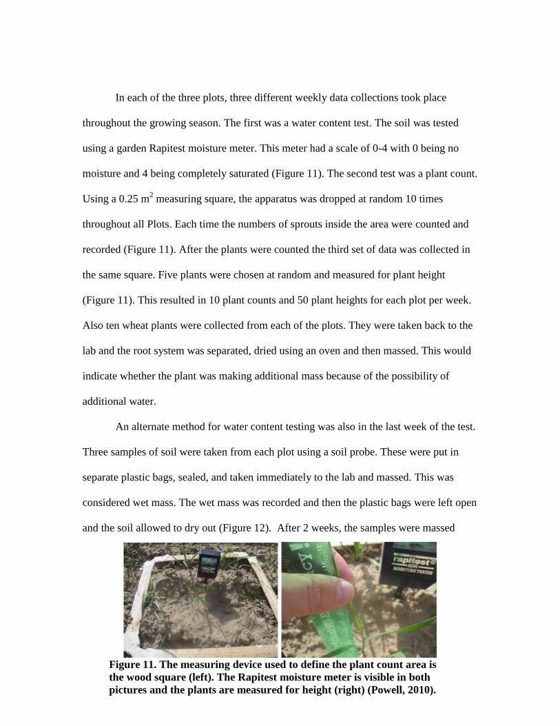
In each of the three plots, three different weekly data collections took place

throughout the growing season. The first was a water content test. The soil was tested

using a garden Rapitest moisture meter. This meter had a scale of 0-4 with 0 being no

moisture and 4 being completely saturated (Figure 11). The second test was a plant count.

Using a 0.25 m2 measuring square, the apparatus was dropped at random 10 times

throughout all Plots. Each time the numbers of sprouts inside the area were counted and

recorded (Figure 11). After the plants were counted the third set of data was collected in

the same square. Five plants were chosen at random and measured for plant height

(Figure 11). This resulted in 10 plant counts and 50 plant heights for each plot per week.

Also ten wheat plants were collected from each of the plots. They were taken back to the

lab and the root system was separated, dried using an oven and then massed. This would

indicate whether the plant was making additional mass because of the possibility of

additional water.

An alternate method for water content testing was also in the last week of the test.

Three samples of soil were taken from each plot using a soil probe. These were put in

separate plastic bags, sealed, and taken immediately to the lab and massed. This was

considered wet mass. The wet mass was recorded and then the plastic bags were left open

and the soil allowed to dry out (Figure 12). After 2 weeks, the samples were massed

Figure 11. The measuring device used to define the plant count area is

the wood square (left). The Rapitest moisture meter is visible in both

pictures and the plants are measured for height (right) (Powell, 2010).

12

Figure 13. A collected tarp sample (on the back of

the combine) about to be transferred to buckets and

later to sacks.(Powell, 2010).

again and recorded as dry mass. The wet mass was divided by the dry mass to find the

percent mass loss in water.

After 136 days, the wheat was harvested for each Plot. A tarp was installed in the

hopper of the combine to catch the wheat from its respective Plot. Each tarped sample

was carefully extracted by lifting and tipping it into grain sacks (Figure 13). This process

was carried out with care, insuring no grain was lost in transition from the combine to

each sack. After each Plot was harvested, the wheat was collected and identified in sacks;

the wheat sacks were weighed to find yield for each Plot.

To calculate the yield, the acreage of the test plots had to be determined. The area

of each of the Plots was 74 m2 (792 ft

2). Since an acre is 4,047 m

2 (43,560 ft

2), the

Figure 12. The drying station in the lab.

Observe the water moisture on the sides of the

bags (Powell, 2010).

13

plots calculated to 0.018 of an acre. To complete the yield calculation, the weights of the

wheat had to be converted into bushels. A bushel is 27.3 kg (60.0 lbs) of wheat. The

masses of the individual plots were divided by the 27.3 kg to get the number of bushels.

The number of bushels in the plots over the acreage of the plots was converted using the

known bushels per acre, 27.3 kg (60 lbs), to find the bushels that would have been

recorded had the plots been full size. Besides yield, kernel counts were taken for the

yield. Random 5.0 g samples of the harvested kernels were retrieved and the individual

kernels counted out. This number was recorded and the process was repeated 10 times for

each Plot’s yield. From that data, the average kernel mass was found by dividing the 5.0

g by the number of kernels.

The local precipitation information was retrieved from weather station at the

Odessa Grange Supply in town. They use an electronic gauge to measure the rainfall and

upload their information to Weather Underground. The annual and the monthly averages

for rainfall were collected and compared to previous years in order to determine if this

could have had an effect on the experiment because of more or less available water

throughout the growing season compared to other years.

All the data was analyzed and t-tests were run to find statistical differences. After

the yield was concluded for each plot the cost effectiveness was calculated to ascertain

whether this product was economically feasible in wide scale farm production.

Results

A soil test was run before the experiment to analyze the chemicals in the soil. The

results showed nitrogen levels at 17 ppm, sulfate at 5 ppm, the phosphorous levels at 30

ppm, and the potassium levels at 708 ppm in the top 0.3 m of soil (Appendix A). Soil

14

tests were run at the conclusion of the test as well. For the Control Plot the nitrogen level

was 3 ppm, the phosphorous at 32 ppm and the potassium at 939 ppm in the top 0.3 m

soil. Sodium was present at 0.12 meq/100g (Appendix B). For the Experimental Plot 1,

the nitrogen level was 4 ppm, the phosphorous level at 36 ppm and the potassium level at

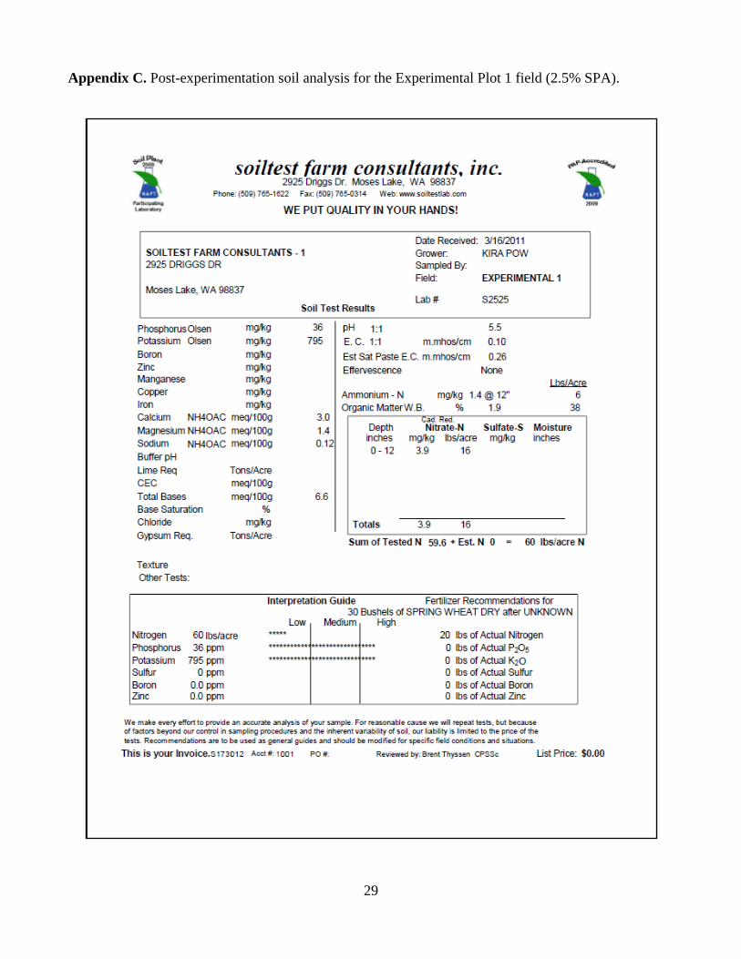
795 ppm. Sodium was present at 0.12 meq/100g (Appendix C). For the Experimental Plot

2, the nitrogen level was 3 ppm, the phosphorous at 31 ppm and the potassium at 844

ppm. Sodium was present at 0.08 meq/100g (Appendix D).

The average wheat height within the Control Plot was 76.0 cm (±4.4) with a high

of 85.0 cm and a low of 65.3 cm. The average wheat height within the Experimental Plot

1 was 81.6 cm (±3.2) with a high of 83.3 cm and a low of 16.8 cm. The average wheat

height within the Experimental Plot 2 was 80.3 cm (±3.7) with the highest individual

sample 90.0 cm and lowest sample 72.0 cm (Table 1). A two tailed t-test was used to

statistically compare the plots. The difference between the average wheat height in

Experimental Plot 1 and the Control Plot was significantly different at the 99.9 %

confidence level (t = ±7.258; df = 98; p < .001). The difference between the average

wheat height in Experimental Plot 2 and Control Plot was significantly different at the

99.9 % confidence level (t = ±5.243; df = 98; p < .001). There was no significant

difference between the average wheat height in Experimental Plot 1 compared to

Table 1. Average Plant Height in the Control Plot, the Experimental Plot 1 and

Experimental Plot 2.

Plot N Ave. Height

(cm)

SD

(cm)

Var.

(cm)

Control Plot 50 76.0 ±4.42 19.5

Experimental Plot 1 50 81.6 ±3.22 10.4

Experimental Plot 2 50 80.3 ±3.77 14.2

15

Experimental Plot 2.

Within the Control Plot the average plant count was 35.0 (±6.6) with the high of

44 and a low of 24. Within the Experimental Plot 1 the average plant count was 41.7

(±2.6) with a high of 46 and a low of 38. Within the Experimental Plot 2, the average

plant count was 38.7 (±9.4) with the high of 57 and a low of 27 (Table 2). A two-tailed t-

test was used to statistically compare the plots. The difference between the average plant

count at harvest in the Control Plot and Experimental Plot 1 was significantly different at

the 95% confidence level (t = ±2.99; df = 18; p<.05). There was no significant difference

between the average plant count in Control Plot and Experimental Plot 2 or between the

average plant count in Experimental Plot 1 and Experimental Plot 2.

Root systems were taken from 10 samples from each plot. The average mass for

the Control Plot was 0.30 g (±.14) with the high of 0.53 g and the low of 0.08 g. The

average mass for the Experimental Plot 1 was 0.56 g (±0.20) with the high of 0.95 g and

the low of 0.28 g. The average root mass for the Experimental Plot 2 was 0.40 g (±.08)

with the high of 0.52 g and the low of 0.29 g (Table 3). A two-tailed t-test was used to

statistically compare the plots. The difference between the average root mass in the

Control Plot and Experimental Plot 1 was significantly different at the 99 % confidence

level (t = ±3.24; df = 18; p < .01).There was no significant difference between the

Table 2. Average Plant Count in the Control Plot, Experimental Plot 1, and Experimental

Plot 2.

Plot N Ave. Count SD Var.

Control Plot 10 35.0 ±6.60 43.56

Experimental Plot 1 10 41.7 ±2.58 6.66

Experimental Plot 2 10 38.7 ±9.41 88.55

16

average root mass in the Control Plot and Experimental Plot 2. The difference between

the average root mass in the Experimental Plot 1 and the Experimental Plot 2 was

significantly different at the 95 % confidence level (t = ±2.33; df = 18; p < .05).

Three soil samples were collected from each of the Plots at a depth of 0.35m (1ft).

They were sealed and taken back to the lab. They were dry and wet massed and the

percent water mass loss was recorded. The average water mass percent lost for the

Control Plot was 1.018 % (±.0004) with the high of 1.066 % and the low of 0.987 %. The

average percent water mass lost for the Experimental Plot 1 was 1.041 % (±.0041) with

the high of 1.508 % and the low of 0.749 %. The average percent water mass lost for the

Experimental Plot 2 was 0.726 % (±.0044) with the high of 1.216 % and the low of

0.341 % (Table 4). A two-tailed t-test was used to statistically compare the plots. There

was no significant difference between the average percent water mass lost in any of the

Plots.

Table 3. Average Root Mass in the Control Plot, Experimental Plot 1 and

Experimental Plot 2.

Plot N Ave. Mass

(g)

SD

(g)

Var.

(g)

Control Plot 10 0.30 ±0.14 0.0196

Experimental Plot 1 10 0.56 ±0.20 0.0400

Experimental Plot 2 10 0.40 ±0.08 0.0059

Table 4. Average Percent Water Mass Lost Between the Control Plot, Experimental

Plot 1 and Experimental Plot 2.

Plot N Ave. % Water

Mass Lost

SD

(%)

Var.

(%)

Control Plot 3 1.018 ±.0004 1.6×10-7

Experimental Plot 1 3 1.041 ±.0041 1.7×10-5

Experimental Plot 2 3 0.726 ±.0044 1.9×10-5

17

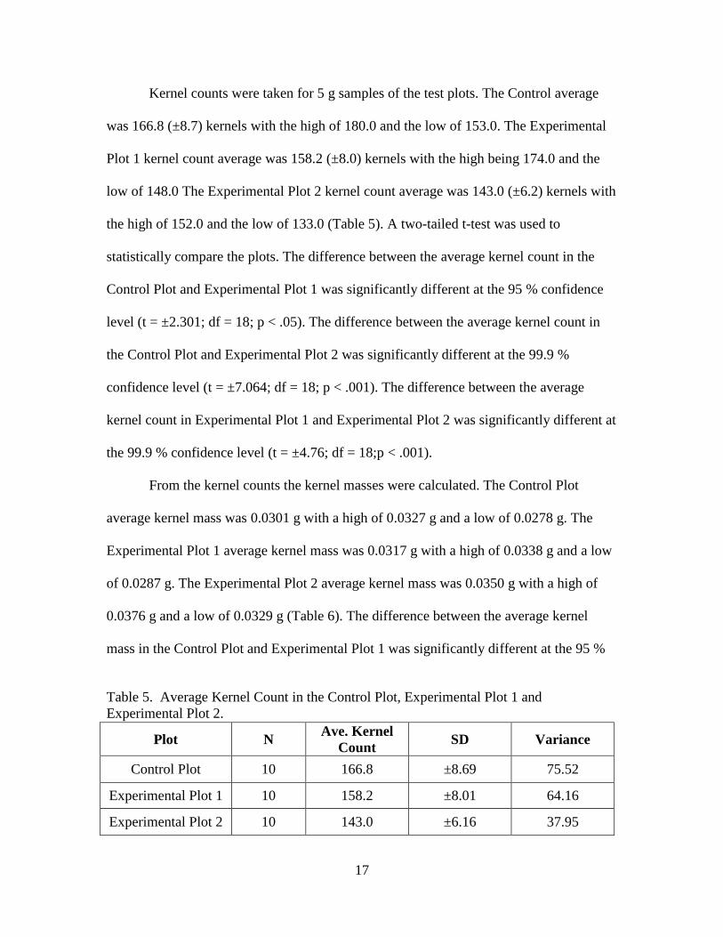
Kernel counts were taken for 5 g samples of the test plots. The Control average

was 166.8 (±8.7) kernels with the high of 180.0 and the low of 153.0. The Experimental

Plot 1 kernel count average was 158.2 (±8.0) kernels with the high being 174.0 and the

low of 148.0 The Experimental Plot 2 kernel count average was 143.0 (±6.2) kernels with

the high of 152.0 and the low of 133.0 (Table 5). A two-tailed t-test was used to

statistically compare the plots. The difference between the average kernel count in the

Control Plot and Experimental Plot 1 was significantly different at the 95 % confidence

level (t = ±2.301; df = 18; p < .05). The difference between the average kernel count in

the Control Plot and Experimental Plot 2 was significantly different at the 99.9 %

confidence level (t = ±7.064; df = 18; p < .001). The difference between the average

kernel count in Experimental Plot 1 and Experimental Plot 2 was significantly different at

the 99.9 % confidence level (t = ±4.76; df = 18;p < .001).

From the kernel counts the kernel masses were calculated. The Control Plot

average kernel mass was 0.0301 g with a high of 0.0327 g and a low of 0.0278 g. The

Experimental Plot 1 average kernel mass was 0.0317 g with a high of 0.0338 g and a low

of 0.0287 g. The Experimental Plot 2 average kernel mass was 0.0350 g with a high of

0.0376 g and a low of 0.0329 g (Table 6). The difference between the average kernel

mass in the Control Plot and Experimental Plot 1 was significantly different at the 95 %

Table 5. Average Kernel Count in the Control Plot, Experimental Plot 1 and

Experimental Plot 2.

Plot N Ave. Kernel

Count SD Variance

Control Plot 10 166.8 ±8.69 75.52

Experimental Plot 1 10 158.2 ±8.01 64.16

Experimental Plot 2 10 143.0 ±6.16 37.95

18

confidence level (t = ±2.33; df = 18; p < .05). The difference between the average kernel

mass in the Control Plot and Experimental Plot 2 was significantly different at the 99.9 %

confidence level (t = ±7.22; df = 18; p < 0.001.). The difference between the average

kernel mass in Experimental Plot 1 and Experimental Plot 2 was significantly different at

the 99.9 % confidence level (t = ±4.84; df = 18;p < 0.001.).

The wheat that was collected from each test plot was massed and the bushels/acre

was calculated using the formula that was mentioned in the Materials and Methods. The

Control Plot raw wheat weighed 13.27 kg (29.2 lbs), which when converted results in

26.8 bushels/acre. The Experimental Plot 1 raw wheat weighed 16.27 kg (35.8 lbs) which

converted into 32.8 bushels/acre. The Experimental Plot 2 raw wheat weighed 16.91 kg

(37.2 lbs), which when converted became 34.1 bushels/acre.

Rainfall was collected for the plots throughout the growing period. Rainfall

observed for the month of April was 4.2 cm. May rainfall totaled 6.1 cm. The rainfall in

June was 4.9 cm. The July rainfall totaled 0.6 cm and the August rainfall totaled 0.9 cm.

The yearly total of rainfall for 2010 was 31.8 cm.

Table 6. Averages Kernel Masses in the Control Plot, Experimental Plot 1 and

Experimental Plot 2

Plot N Ave. Kernel

Mass (g) SD Variance

Control Plot 10 0.0301 ±0.00156 2.43E-6

Experimental Plot 1 10 0.0317 ±0.00157 2.46E-6

Experimental Plot 2 10 0.0350 ±0.00152 2.31E-6

19

Discussion

The hypothesis was accepted because the plant height, kernel, and yield results

supported the theory that the sodium polyacrylate’s addition to the soil resulted in

increased crop growth and production.

The soil chemical test in the preliminary part of the planting stage showed that the

levels of nutrients in the soil were adequate for crop growth. Because the parts per

million fell between 2 ppm and 60 ppm, the level of phosphorus was classified as high

and because the potassium level was between 50 ppm and 700 ppm, it was classified as

very high. High levels of these minerals is not a negative, it is beneficial. These tests

revealed the soil was full of nutrients needed for crop production.

The post-test soil data showed the sodium polyacrylate had no apparent negative

effect on the soil. The nitrogen levels dropped from 5 ppm to 3 pmm, 4 ppm and 3 ppm

for the Control, Experimental Plot 1 and Experimental Plot 2 respectively but this can be

expected from a normal growth sequence.

The plant height data supported the hypothesis because the Control Plot was

significantly different then both the Experimental Plot 1 and the Experimental Plot 2.

This revealed that the sodium polyacrylate caused the wheat to grow higher. The growing

trend of the wheat was compared to the time (in days) for each of the three Plots. As seen

by the R2 values, the plants in the Control Plot (R

2=.991) (Figure 14), Experimental Plot

1 (R2=.970) (Figure 15), and Experimental Plot 2 (R

2=.995) (Figure 16) all grew

normally, yet the Experimental Plot 1 and Experimental Plot 2 grew with significantly

higher averages than the Control Plot. This supports the hypothesis that the addition of

the sodium polyacrylate increased crop growth.

20

The kernel counts also supported the hypothesis. The Control Plot count of 166.8

was significantly different at the 95 % confidence level from the Experimental Plot 1 and

the reduced number of kernels in the 5.0 g sample for the Experimental Plot 1 and

Experimental Plot 2 allude to the fact that the individual kernels weigh more themselves

(Figure 17).

The Control Plot kernels weighed an average of 0.0301 g, the Experimental Plot 1

kernels weighed an average of 0.0316 g and the Experimental Plot 2 kernels weighed an

average of .0350 g (Figure 18). The Experimental Plot 1 kernels weighed

1.1 % more than the Control Plot kernels and the Experimental Plot 2 kernels weighed

1.2 % more than the Control Plot kernels Higher kernel mass contributes to higher yields

and higher test weights, which are desirable, (Squires, 2011). According to the

Figure 14. The Average Control Plot Wheat Height (cm) Through Time (days).

21

Washington Grain Commission, the higher average kernel mass of the Experimental Plots

means processed, more flour would be produced as compared to the Control. Overall, the

kernels contain more usable substance. Even though the kernels do not contain any more

nutrients or protein, the bigger size is desirable because it increases yield. Kernels also

indicate how stressful the growing season was on the plants. When kernels are large and

heavy, it means they had plenty of the requirements needed for healthy growth, light,

nutrients and most of all water. Water availability and kernel size are directly linked

(Engle, 2011). The results of this test show that water was available for the plant

throughout the growing season which was the focus of this research.

The calculated yields for the three plots were truly the indicator of whether the

sodium polyacrylate was successful in retaining water. The Control Plot yielded 26.8

Figure 15. The Average Experimental Plot 1 Wheat Height (cm) Through Time (days).

22

bushels/acre. The Experimental Plot 1 yielded 32.8 bushels/acre which was a 22 %

increase from the Control Plot. The Experimental Plot 2 yielded 34.1 bushels/acre which

was a 27 % increase from the Control Plot. These percents are significant because

farmers are looking for ways to increase their crop and if sodium polyacrylate provides at

least a 20 % increase in raw yield, then it can be applicable in large scale farming.

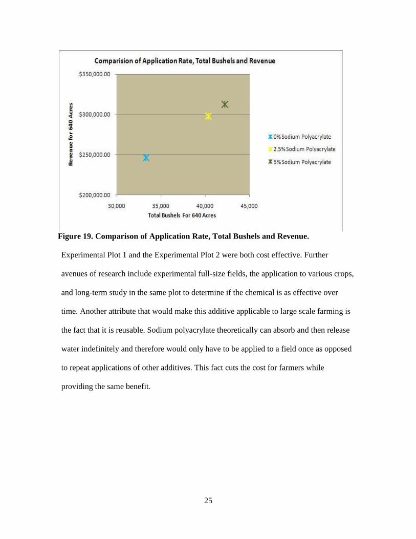
Although the yield increase is interesting it is the cost effectiveness that is truly

astounding. The current price of grain is $7.41 per bushel (Odessa Union, 2011). A 640

acre field (one square mile also called a section) without sodium polyacrylate would

harvest approximately 52 bushel/acre (the state average for spring wheat in 2010)

resulting in a total of 33,280 bushels (Knopf, 2010). If this was multiplied by the price of

one bushel, there would be a gross of $246,605. If the same field was treated with a 0.68

kg (1.5 lbs) per acre application rate of sodium polyacrylate, there should be an expected

Figure 16. The Average Experimental Plot 1 Wheat Height (cm) Through Time (days).

23

0

20

40

60

80

100

120

140

160

180

200

Average Kernel Count

Nu

mb

er

of

See

ds

Average Kernel Count

Control Plot

Experimental Plot 1

Experimental Plot 2

22% increase in bushels/acre (as shown in Experimental Plot 1 and Plot 2). This would

increase harvest to a rate of 63 bushels/acre, which translates into 40,320 total bushels or

$298,771. That is an increase of $52,166 in revenue. If you take out the cost of the

sodium polyacrylate to seed that same area ($531) then the revenue increase would be

$51,635 and the gross total would be $298,240. The use of the 1.36 kg (3.0 lbs)

application rate was also cost effective. It resulted in 66 bushel/acre harvest (27 %

increase), 42,240 total bushels, $312,998 gross, and a $65,337 revenue increase (cost of

sodium polyacrylate would be $1056) (Figure 19).

It is noted that the bushels per acre for all three of the plots were lower than the

average yield for dry-land farming in the area. This could be due to the contraction of a

stripe rust infection on June 25. Stripe rust is a fungus that infects the leaf part of the

wheat plant producing yellow, orange uredospores. If left untreated, the fungus will

Figure 17. Average Kernel Count Comparison for the Control Plot, Experimental

Plot 1 and Experimental Plot 2, with Standard Deviation.

24

completely overrun the plant and the wheat will die. However, the variety used for this

test had been genetically modified to contain a gene that is activated by heat to stop the

rust infection. At the initial onset of the infection, the weather was not quite hot enough

to stop the spread but over the next week the temperature heated up to activate the

resistance gene thus halting the infection. Because of the delay in the stoppage of the

infection, the rust could have affected the overall yield by harming the wheat. Also, it

was observed that the severity of the infection was the same throughout the three plots

and therefore should have affected the respective plot yields equally. Without the

infection the yields of the three Plots would likely have been higher.

In conclusion, the hypothesis was accepted. The application of sodium

polyacrylate increased crop growth in dry-land farming, as shown through the improved

average height, kernel count/mass, and yield results. It increased the bushels/acre by at

least 20 %. For farmers this is a highly attractive figure. The application rates used in the

Figure 18. Average Kernel Mass Comparison for the Control Plot, Experimental

Plot 1 and Experimental Plot 2, with Standard Deviation.

25

Experimental Plot 1 and the Experimental Plot 2 were both cost effective. Further

avenues of research include experimental full-size fields, the application to various crops,

and long-term study in the same plot to determine if the chemical is as effective over

time. Another attribute that would make this additive applicable to large scale farming is

the fact that it is reusable. Sodium polyacrylate theoretically can absorb and then release

water indefinitely and therefore would only have to be applied to a field once as opposed

to repeat applications of other additives. This fact cuts the cost for farmers while

providing the same benefit.

Figure 19. Comparison of Application Rate, Total Bushels and Revenue.

26

Acknowledgements

I would like to thank Mr. Jeff Schibel for the use of his land, equipment, and seed

as well as farming advice for an amateur as the study progressed. Also, I would like to

acknowledge my parents, Steven and Linda Powell for helping with transportation and

encouragement. I would like to thank Soiltest Farm Consultants, Inc. for graciously

providing free soil analysis for my research. Lastly, I would like to thank my science

teacher, Mr. Wehr for all his assistance in all stages of the project, from the initial idea on

paper to the completion of this paper, his help was invaluable.

27

Appendix A. Pre-experimentation soil analysis for the Control, Experimental Plot 1, and

Experimental Plot 2 fields.

28

Appendix B. Post-experimentation soil analysis for the Control field.

29

Appendix C. Post-experimentation soil analysis for the Experimental Plot 1 field (2.5% SPA).

30

Appendix D. Post-experimentation soil analysis for the Experimental Plot 2 field (5.0% SPA).

31

References & Literature Cited

Absorbent Technologies. (2009). How it Works: Unique Composition Promotes Healthy

Microenvironment. ZEBA Informational Site, Absorbent Technologies, (1/20/11).

Bouma, J. (2009). Retention of Water: Basics of Soil-Water Relationships-Part II.

University of Florida IFAS Extension, www.edis.ifas.ufl.edu/ss109, (12/06/10).

Bryant, K. (2008). Australian Food Bowl Lies Empty. BBC News, www.bbc.co.uk,

(12/03/10).

Engle, D. (2011). Phone Discussion Relating to Kernel Mass Significance, Western

Wheat Quality Laboratory, Pullman, WA, (2/9/11).

France, C. (2008). Products from Oil; Polymers. GCSE Science Chemistry High School,

http://www.gcsescience.com/o70.htm, (12/01/10).

Gesell, S.G. (2000). Hessian Fly on Wheat. Penn State Entomology Fact Sheet, Penn

State University, www.ento.psu.edu, (10/21/10).

Harrison, S. (2003). Soil Formulation for Resisting Erosion. United States Patent

Application Publication, (10/23/09).

Hayes, M.J. (2004). Estimating the Economic Impacts of Drought. American

Metrological Association, (12/11/09).

Inglis, D.A. (1993). Small Grain Disease-Stripe Rust. Washington State University

Bulletin, Washington State University, (10/21/10).

Kidwell, K. (2005). Registration of Louise Wheat. Agricultural Research Service, United

States Department of Agricultural, www.ars.usda.gov, (9/21/10).

Knopf, D. (2010). Washington Wheat Production 2010 up 22 Percent from Last Year.

National Agricultural Statistics Service, United State Department of Agricultural,

www.nass.usda.gov, (2/9/11).

Lang, S.S. (2006). Slow, insidious' soil erosion threatens human health and welfare as

well as the environment, Cornell study asserts. Chronicle Online, Cornell

University, Ithaca, IN, (11/16/09).

Livingston, J. (2010). Phone Conversation Pertaining to Precipitation Levels in Lincoln

County. Meteorologist. Spokane Branch of the National Weather Service,

Spokane, WA, (9/2/10).

Monatana, S. (2009). Facts About the Dust Bowl. www.factoidz.com, (12/4/09).

32

NDMC. (2006). What is Drought? Understanding and Defining Drought. National

Drought Mitigation Center, University of Nebraska-Lincoln, Lincoln, NE,

(10/26/09).

NIVAP, (2010). Water Retention Curve Graphic. Netherlands Potato Consultative

Foundation, http://www.aardappelpagina.nl/uk, (2/11/11).

NRCS. (2009). Web Soil Survey. National Resources Conservation Service, United States

Department of Agriculture, http://websoilsurvey.nrcs.usda.gov, (2/10/11).

National Weather Service, (2010). Rainfall Level Data. http://www.nws.noaa.gov/

(9/2/10)

Odessa Union, (2011). Current Grain Prices. Odessa Union Warehouse Co-Op, Odessa,

WA, (1/22/11).

Piako Tractors. (2009). Einbock Air Seed Box Universal. Piako Tractors and Equipment

website, http://www.piakotractors.co.nz, (1/20/11).

Richer Consulting Services, (2007), What Are the Components of Typical Disposable

Diapers?, Frequently Asked Questions about Disposable Diapers,

www.disposable diapers.net, (2/10/11).

Rosencrans, M. (2009). U.S Drought Monitor. National Drought Mitigation Center,

University of Nebraska-Lincoln, Lincoln, NE, (11/20/09).

Schillinger, W. (2010). Email Discussion Relating to the Water Retention Curve. Soil

Scientist. Washington State University, (01/06/10).

Schibel, J. (2010). Direct Discussion Relating to Plot Site, Odessa, WA, (3/24/10)-

(9/20/10).

Smith, T. (2008). Food Crisis: Drought Hurts Vital Australian Wheat. USA Today

Online, www.usatoday.com, (12/03/10).

Squires, G. (2011). Phone Discussion Relating to Kernel Mass Significance, Washington

Grain Commissioners, Spokane, WA, (2/9/11).

USDA. (2008). National Agricultural Statistics Service. United States Department of

Agriculture, (12/15/09).

ZGEPTC, (2011). Bulk Pricing for Sodium Polyacrylate. Zhengzhou Guangyang

Environmental Protection Technology Co., Ltd., product information,

www.alibaba.com, (2/10/11).