Embed Size (px)
Citation preview
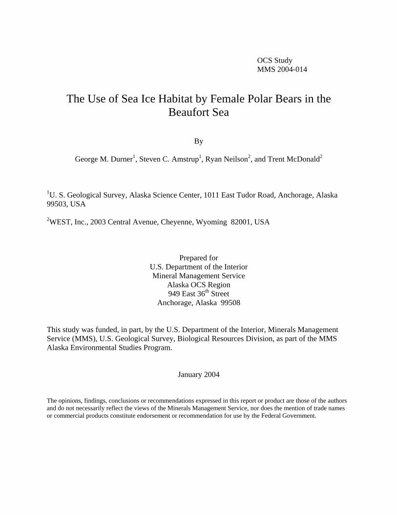
OCS Study MMS 2004-014
The Use of Sea Ice Habitat by Female Polar Bears in the Beaufort Sea
Prepared for U.S. Department of the Interior Mineral Management Service
Alaska OCS Region 949 East 36th Street
Anchorage, Alaska 99508
OCS Study MMS 2004-014
The Use of Sea Ice Habitat by Female Polar Bears in the Beaufort Sea
By
George M. Durner1, Steven C. Amstrup1, Ryan Neilson2, and Trent McDonald2
1U. S. Geological Survey, Alaska Science Center, 1011 East Tudor Road, Anchorage, Alaska 99503, USA 2WEST, Inc., 2003 Central Avenue, Cheyenne, Wyoming 82001, USA
Prepared for
U.S. Department of the Interior Mineral Management Service
Alaska OCS Region 949 East 36th Street
Anchorage, Alaska 99508
This study was funded, in part, by the U.S. Department of the Interior, Minerals Management Service (MMS), U.S. Geological Survey, Biological Resources Division, as part of the MMS Alaska Environmental Studies Program.
January 2004
The opinions, findings, conclusions or recommendations expressed in this report or product are those of the authors and do not necessarily reflect the views of the Minerals Management Service, nor does the mention of trade names or commercial products constitute endorsement or recommendation for use by the Federal Government.
PROJECT ORGANIZATION PAGE George M. Durner, Research Zoologist, U.S. Geological Survey, Alaska Science Center, 1011 East Tudor Road, Anchorage, Alaska 99503, USA Steven C. Amstrup, Project Leader, U.S. Geological Survey, Alaska Science Center, 1011 East Tudor Road, Anchorage, Alaska 99503, USA Ryan Nielson, Statistician, WEST, Inc., 2003 Central Avenue, Cheyenne, Wyoming 82001, USA Trent McDonald, Statistician, WEST, Inc., 2003 Central Avenue, Cheyenne, Wyoming 82001, USA REPORT AVAILABILITY U.S. Geological Survey Alaska Science Center 1011 East Tudor Road Anchorage, AK 99503 Telephone: (907) 786-3512 SUGGESTED CITATION Durner, G. M., S. C. Amstrup, R. Neilson, and T. McDonald. 2004. The Use of Sea Ice Habitat
by Female Polar Bears in the Beaufort Sea. U.S. Geological Survey, Alaska Science Center, Anchorage, Alaska. OCS study, MMS 2004-014.
ii
TABLE OF CONTENTS PROJECT ORGANIZATION PAGE.............................................................................................II
TABLE OF CONTENTS.............................................................................................................. III
LIST OF TABLES........................................................................................................................ IV
LIST OF FIGURES ....................................................................................................................... V
ABSTRACT.................................................................................................................................. VI
ACKNOWLEDGEMENTS.........................................................................................................VII
INTRODUCTION .......................................................................................................................... 1
METHODS ..................................................................................................................................... 2
...................................................................................................................................... 3Ice Data
............................................................................................................................... 6Ocean Depth
............................................................................................. 6Creating Discrete Choice Habitats
.................................................................................................................. 6Polar Bear Locations
................................................................................ 7Defining Habitat Available to Polar Bears
.............................................. 8Generating Random Locations and Attaching Habitat Variables
................................................................................ 8Generating a Resource Selection FunctionRESULTS ....................................................................................................................................... 9
....................................................................................................................................... 10Spring
.................................................................................................................................... 11Summer
.................................................................................................................................... 13Autumn
...................................................................................................................................... 14Winter
............................................................................................................... 14Evaluation of ModelsDISCUSSION............................................................................................................................... 16
LITERATURE CITED ................................................................................................................. 21
APPENDICES .............................................................................................................................. 25
iii

LIST OF TABLES Table 1. Descriptions and codes for ice stage and form………………………………………..4 Table 2. Original codes for National Ice Center ice concentration…………………………….6 Table 3. Seasonal discrete choice models predicting relative probability…………………….10
iv
LIST OF FIGURES Figure 1. Extent of the National Ice Center ice chart of the Beaufort Sea Figure 2. Example of movements of bear 20330 Figure 3. Defined seasons for modeling polar bear habitat use Figure 4. Relative probability of selection as a function of variables – spring Figure 5. Relative probability of selection as a function of variables – summer Figure 6. Relative probability of selection as a function of variables – autumn Figure 7. Relative probability of selection as a function of variables – winter Figure 8. Comparing the seasonal distribution of RSF values in the Beaufort Sea Figure 9. Distribution of the spring RSF in the Beaufort Sea – June Figure 10. Distribution of the spring RSF in the Beaufort Sea – February
v
ABSTRACT Polar bears (Ursus maritimus) depend on ice-covered seas to satisfy life history
requirements. Modern threats to polar bears include oil spills in the marine environment and changes in ice composition resulting from climate change. Managers need practical models that explain the distribution of bears in order to assess the impacts of these threats. We explored the use of discrete choice models to describe habitat selection by female polar bears in the Beaufort Sea. Using stepwise procedures we generated resource selection models of habitat use. Sea ice characteristics and ocean depths at known polar bear locations were compared to the same features at randomly selected locations. Models generated for each of four seasons confirmed complexities of habitat use by polar bears and their response to numerous factors. Bears preferred shallow water areas where different ice types intersected. Variation among seasons was reflected mainly in differential selection of total ice concentration, ice stages, floe sizes, and their interactions. Distance to the nearest ice interface was a significant term in models for three seasons. Water depth was selected as a significant term in all seasons, possibly reflecting higher productivity in shallow water areas. Preliminary tests indicate seasonal models can predict polar bear distribution based on prior sea ice charts and bathymetry data. KEY WORDS: discrete choice models, habitat selection, polar bear, resource selection function, RSF, sea ice, Ursus maritimus.
vi
ACKNOWLEDGEMENTS Principal funding for this work was provided by the United States Geological Survey, Alaska Science Center, and the United States Minerals Management Service. Additional support was provided by the following agencies: BP Exploration – Alaska, Inc.; the Canadian Wildlife Service, Edmonton, Alberta; ConocoPhillips Alaska, Inc.; Continental Shelf Project, Ottawa, Ontario; ExxonMobil, Corp.; U.S. Fish and Wildlife Service, Marine Mammals Management; North Slope Borough, Department of Wildlife Management; and the Northwest Territories Department of Resources, Wildlife and Economic Development, Inuvik, NWT. We thank the following for their support in the field and office: Air Logistics-Alaska, Arctic Air Alaska, D. Andriashek, M. Branigan, A. Fischbach, K. Simac and G. Weston-York. D. Douglas provided support in satellite-telemetry data processing. The following individuals provided constructive reviews on an earlier draft of this manuscript: E. Knudsen, W. Horowitz, M. Huso, K. Simac, I. Stirling, and one anonymous referee.
vii
INTRODUCTION
Polar bears (Ursus maritimus) occur in most ice-covered seas throughout the Arctic basin (Amstrup 2003). Their range includes the southern Beaufort Sea of northern Alaska and the Chukchi and Bering Seas of western Alaska. This dependence on sea ice is so strong that the distribution of polar bear sub-populations may be determined by regional characteristics of the sea ice (Ferguson et al. 1998). While the presence of sea ice is a prerequisite, bears probably respond to a multitude of ice characteristics and the interaction of those characteristics (Stirling et al. 1993). Polar bears depend on sea ice for hunting ringed (Phoca hispida) and bearded seals (Erignathus barbatus) (Stirling et al. 1993). Seal abundance and distribution in the southern Beaufort Sea is assumed to be dependent on the seasonal and annual variability of ice characteristics (Kelly 1988) and ecosystem productivity (Stirling and Oritsland 1995). While high prey density may be tied to areas of high seasonal variability in sea ice, the nature of ice may actually decrease polar bear access to prey (Ferguson et al. 2000). Female bears with new young are believed to utilize the stable nearshore fast ice in order to avoid adult males and to hunt seals occupying subnivian birth lairs (Stirling et al. 1993). The degree of success in locating mates during the breeding season may be dependent on ice type (Stirling et al. 1993). Annual dynamics of sea ice result in a pulse of polar bears into the near-shore regions of autumn ice. Access to terrestrial maternal den habitat may be dependent on autumn sea ice characteristics (Stirling and Andriashek 1992, Amstrup and Gardner 1994). In the Beaufort Sea region as many as 50% of pregnant bears give birth to their young in snow dens on the surface of the sea ice (Amstrup and Gardner 1994). Maternal dens in the pelagic environment depend on stable ice for the duration of den tenure (Amstrup and Gardner 1994). In summary, polar bear distribution is not uniform in the Arctic but rather is determined by the nature, spatial and temporal extent of sea ice, and the specific requirements of reproductive status.
Sea ice is composed of a complex array of ever changing structure and composition (MANICE 1994). The action of currents, winds and temperatures, which vary by season, produce a range of ice composition including rafts of new ice only several centimeters thick to pressure ridges of first year and old ice that rise several meters above and below the sea surface. Pack ice leads form and close and floes of various sizes are created. Some ice survives the summer’s melt to become thick and stable multiyear ice. Polar bears are the apical predator of this environment. Perceived changes in population status and distribution of polar bears may be extrapolated to determine effects due to variation in the sea ice environment (Stirling and Derocher 1993, Stirling 1997). Conversely, observed and predicted changes in sea ice patterns may be used to estimate the future effects on polar bears. The relationship between polar bears and their primary prey, i.e., ringed seals, is so close that understanding the population status of one can be used to explain the population status of another (Stirling and Øritsland 1995). On the next level, because productivity of ringed seals is closely tied to the productivity of arctic marine systems, knowledge of polar bear population status and distribution may provide an understanding of variation in productivity in arctic seas (Stirling and Derocher 1993, Stirling 1997). In oceans where sea ice is prevalent throughout most of the year, biological productivity is likely driven by presence of the continental shelf, ice edge habitat, and waters fed by nearshore polynyas (Stirling 1997). Ultimately, however, both prey and predator populations are driven by the nature of the sea ice (Stirling et al. 1977, Mauritzen et al. 2003).
Understanding the relationship between polar bears and sea ice is useful from a management perspective. Future industrial development along the northern Alaska coast is expected to extend further into polar bear habitat and will increase the potential for
1
anthropogenic disturbances (Amstrup et al. 1986). Off-shore petroleum exploration and development and ocean-going vessels can alter sea-ice habitat and thus polar bear distribution (Amstrup et al. 1986, Stirling 1990). Petroleum spills can be directly fatal to polar bears or result in long-term negative health effects (Øritsland et al. 1981, St. Aubin 1990). Spilled oil will most likely accumulate in habitats frequented by seals and polar bears (Neff 1990). Evidence suggests that arctic climate patterns are changing (Vinnikov et al. 1999, Morison et al. 2000, Parkinson 2000, Drobot and Maslanik 2002). Slight increases in average temperatures may cause dramatic changes in the sea ice on which polar bears depend. Long-term absence of sea ice will negatively impact polar bear populations (Stirling et al. 1999). One effect may include local extinction within the southern periphery of their range (Stirling and Derocher 1993, Stirling et al. 1999). The welfare of polar bears is an international and local concern (Lentfer 1974, Nageak et al. 1991). Addressing this concern will necessitate a greater understanding of polar bear habitat use in order to prevent or mitigate negative consequences from environmental perturbations.
We have a sound understanding of the population status and distribution of polar bears in the Beaufort Sea (Amstrup et al. 2000, Amstrup et al. 2001a, Amstrup et al. 2001b). Other agencies have developed protocols for accurate mapping of sea ice through compiling various remotely sensed and in situ data sources (MANICE 1994, Partington et al. 1999). Considerable gains have been made in understanding polar bear and sea ice relationships in other regions of the Arctic (Ferguson et al. 2000, Mauritzen et al. 2001, 2003) but not, however, in the Beaufort Sea. In particular, the coarse resolution of previous studies has been inadequate to explain the fine-scale aspects of sea ice habitat use (Arthur et al. 1996, Mauritzen et al. 2003). A need exists for practical models of polar bear/sea ice relationships that managers may use to assess the impacts of anthropogenic and natural changes in the Arctic. The ability to predict the response of polar bears to a changing Arctic and to reduce the potential negative effects of human-caused perturbations will increase with a better understanding of polar bear sea ice requirements.
The objective of this study was to quantitatively describe patterns of sea ice-habitat use by polar bears in the southern Beaufort Sea. Furthermore, the products of this study provide the tools that allow resource agencies to predict the likelihood of occurrence of polar bears within a region based on the characteristics of the sea ice. Historical distributions of ice may be used to predict occurrence of polar bears prior to initiation of proposed human activity. Updates of sea ice charts will allow managers to adjust management plans according to changes in sea ice composition and the expected polar bear distribution that results. In this study we used discrete choice models to quantify patterns of sea ice habitat use by polar bears in the Beaufort Sea. We tested the performance of our models against an independent set of real polar bear location data. The practical application of this knowledge will allow managers to predict occurrence of polar bears and create flexible management plans prior to initiation of proposed human activities.
METHODS
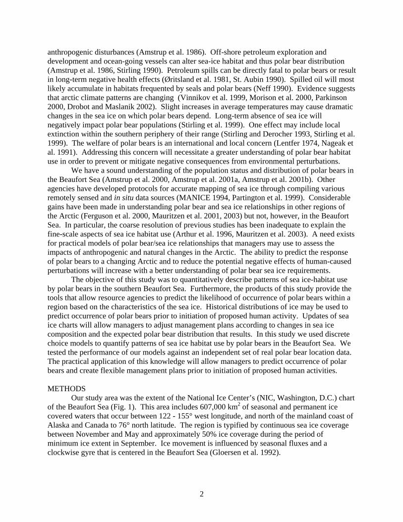
Our study area was the extent of the National Ice Center’s (NIC, Washington, D.C.) chart of the Beaufort Sea (Fig. 1). This area includes 607,000 km2 of seasonal and permanent ice covered waters that occur between 122 - 155° west longitude, and north of the mainland coast of Alaska and Canada to 76° north latitude. The region is typified by continuous sea ice coverage between November and May and approximately 50% ice coverage during the period of minimum ice extent in September. Ice movement is influenced by seasonal fluxes and a clockwise gyre that is centered in the Beaufort Sea (Gloersen et al. 1992).
2
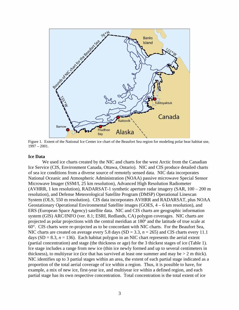
Figure 1. Extent of the National Ice Center ice chart of the Beaufort Sea region for modeling polar bear habitat use, 1997 – 2001. Ice Data
We used ice charts created by the NIC and charts for the west Arctic from the Canadian Ice Service (CIS, Environment Canada, Ottawa, Ontario). NIC and CIS produce detailed charts of sea ice conditions from a diverse source of remotely sensed data. NIC data incorporates National Oceanic and Atmospheric Administration (NOAA) passive microwave Special Sensor Microwave Imager (SSM/I, 25 km resolution), Advanced High Resolution Radiometer (AVHRR, 1 km resolution), RADARSAT-1 synthetic aperture radar imagery (SAR, 100 – 200 m resolution), and Defense Meteorological Satellite Program (DMSP) Operational Linescan System (OLS, 550 m resolution). CIS data incorporates AVHRR and RADARSAT, plus NOAA Geostationary Operational Environmental Satellite images (GOES, 4 – 6 km resolution), and ERS (European Space Agency) satellite data. NIC and CIS charts are geographic information system (GIS) ARC/INFO (ver. 8.1; ESRI, Redlands, CA) polygon coverages. NIC charts are projected as polar projections with the central meridian at 180º and the latitude of true scale at 60°. CIS charts were re-projected as to be concordant with NIC charts. For the Beaufort Sea, NIC charts are created on average every 5.8 days (SD = 3.3, n = 265) and CIS charts every 11.1 days (SD = 8.3, n = 136). Each habitat polygon in an NIC chart represents the aerial extent (partial concentration) and stage (the thickness or age) for the 3 thickest stages of ice (Table 1). Ice stage includes a range from new ice (thin ice newly formed and up to several centimeters in thickness), to multiyear ice (ice that has survived at least one summer and may be > 2 m thick). NIC identifies up to 3 partial stages within an area, the extent of each partial stage indicated as a proportion of the total aerial coverage of ice within a region. Thus, it is possible to have, for example, a mix of new ice, first-year ice, and multiyear ice within a defined region, and each partial stage has its own respective concentration. Total concentration is the total extent of ice
3
Table 1. Descriptions and codes for ice stage and form for generating polar bear resource selection functions in the Beaufort Sea, 1997 – 2001. National Ice Center Ice stage Thickness
(cm) NIC code Our code
for stage Ice free 00 Ice free No stage 80 Ice free New 81 Ice free Nilas, rind < 10 82 Ice free Young 10 – 30 83 Young Grey 10 – 15 84 Young Grey – white 10 – 30 85 Young 1st year 30 – 200 86 First year Thin 1st year 30 – 70 87 First year Thin 1st year stage 1
30 – 50 88 First year
Thin 1st year stage 2
50 – 70 89 First year
Medium 1st year
70 – 120 91 First year
Thick 1st year ice
> 120 93 First year
Old ice 95 Old 2nd year 96 Old Multi-year 97 Old Canadian Ice Service Form description
Width (m)
CIS code Our code for form
Pancake < 2 0 Cake Small cake ice < 2 1 Cake Ice cake 2 – 20 2 Cake Small floe 20 – 100 3 Small floe Medium floe 100 – 500 4 Small floe Big floe 500 – 2000 5 Big floe Vast floe 2000 – 10,000 6 Vast floe Giant floe > 10,000 7 Vast floe Fast ice 8 Fast ice coverage (expressed in tenths), and is the sum of concentrations of the 3 partial stages within the respective region (Table 2). Likewise, CIS charts delineate habitat polygons of the partial concentration and form (average floe size) of ice. Ice form is defined as a categorical average size (diameter) of individual ice floes within an area (Table 1). Ice form can range from small ice cakes that average 2 m in diameter, to giant ice floes that may be > 10 km in diameter. For example, an ice form coded as “2” indicates “cake ice” that is 2 – 20 m in diameter. Likewise, an ice form coded as “5” indicates “big floes” that range between 500 – 2000 m in diameter.
4
Each partial ice form has an accompanying partial concentration. As with ice stage, CIS data identifies as many as 3 partial ice forms within a defined region, the extent of each one a proportion of total area. Because we used NIC charts for determining partial and total concentrations, we re-calculated the extent (concentration) of CIS partial ice forms so that their sum would be equal to total concentration derived from NIC charts. We binned similar ice stages and similar ice forms to simplify models (Table 1).
Both NIC and CIS present data of ice concentration, stage and form as categorical variables. With NIC data, a single code is used to represent a range of values. For example, consider the following NIC code for an ice polygon:
CT91CA809599CB108399CC018199.
In this example the 1st 4 columns (CT91) represents the total extent of ice cover, which is 90 – 100% cover. The first thickest partial stage is represented by columns 5 – 12, where the partial ice concentration is ‘80’ (80% coverage), the stage of ice is ‘95’ (old ice), and the ice form is ‘99’ (unknown). The 2nd thickest partial stage is represented by columns 13 – 20, where the partial concentration is ‘10’ (10 % coverage), the stage is ‘83’ (young ice, 10 – 30 cm thick), and the form is ‘99’ (unknown). The 3rd thickest stage is represented by columns 21 – 28, where the partial concentration is ‘01’ (< 10 % coverage), the stage is ‘81’ (new ice < 10 cm thick), and the form is unknown. We converted NIC categorical values of partial concentration into continuous variables by simply defining concentrations as the midpoint of the concentration range of the NIC category. Using the character string presented in the prior example, the 1st, 2nd and 3rd partial concentrations would be 0.80, 0.10, and 0.05, respectively. Total concentration is set to the sum of these partial concentrations, or 0.95. Converting categorical variables into continuous variables can introduce bias into model parameter estimates. This generally is not a problem, however, when the original values are continuous in nature, and have been binned into categories after data collection (binned by NIC and CIS). Distance to the nearest polygon edge of NIC charts (edge) was also calculated. The category edge denotes the change of one NIC ice polygon to another adjacent ice polygon and is not to be confused with a transition from ice to relatively open water (Ferguson et al. 2000, Mauritzen et al. 2003). Because of the many different combinations of ice polygons that would produce an ice interface, we did not attempt to categorize ice interface types.
Both NIC and CIS data offer several advantages in modeling polar bear sea ice relationships. They provide a far higher resolution picture than previously available over large areas (Arthur et al. 1996, Mauritzen et al. 2003). Maps are generated from diverse remotely sensed data that are interpreted to provide information on total ice concentration, as well as partial ice stages and forms. NIC and CIS charts are almost real time data. The extent of both NIC and CIS data includes the entire distribution of polar bears in the world. Thus, near real time analysis of expected polar bear distribution anyplace in the polar basin may be possible by modeling NIC and CIS data. Lastly, these data are interpreted and readily available to researchers and resource managers.
5
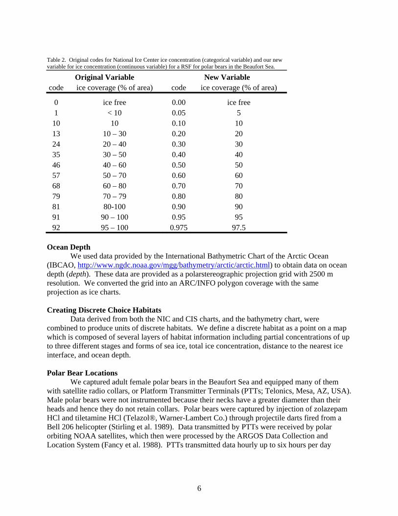
Table 2. Original codes for National Ice Center ice concentration (categorical variable) and our new variable for ice concentration (continuous variable) for a RSF for polar bears in the Beaufort Sea.
Original Variable New Variable code ice coverage (% of area) code ice coverage (% of area)
0 ice free 0.00 ice free 1 < 10 0.05 5 10 10 0.10 10 13 10 – 30 0.20 20 24 20 – 40 0.30 30 35 30 – 50 0.40 40 46 40 – 60 0.50 50 57 50 – 70 0.60 60 68 60 – 80 0.70 70 79 70 – 79 0.80 80 81 80-100 0.90 90 91 90 – 100 0.95 95 92 95 – 100 0.975 97.5
Ocean Depth We used data provided by the International Bathymetric Chart of the Arctic Ocean (IBCAO, http://www.ngdc.noaa.gov/mgg/bathymetry/arctic/arctic.html) to obtain data on ocean depth (depth). These data are provided as a polarstereographic projection grid with 2500 m resolution. We converted the grid into an ARC/INFO polygon coverage with the same projection as ice charts. Creating Discrete Choice Habitats Data derived from both the NIC and CIS charts, and the bathymetry chart, were combined to produce units of discrete habitats. We define a discrete habitat as a point on a map which is composed of several layers of habitat information including partial concentrations of up to three different stages and forms of sea ice, total ice concentration, distance to the nearest ice interface, and ocean depth. Polar Bear Locations We captured adult female polar bears in the Beaufort Sea and equipped many of them with satellite radio collars, or Platform Transmitter Terminals (PTTs; Telonics, Mesa, AZ, USA). Male polar bears were not instrumented because their necks have a greater diameter than their heads and hence they do not retain collars. Polar bears were captured by injection of zolazepam HCl and tiletamine HCl (Telazol®, Warner-Lambert Co.) through projectile darts fired from a Bell 206 helicopter (Stirling et al. 1989). Data transmitted by PTTs were received by polar orbiting NOAA satellites, which then were processed by the ARGOS Data Collection and Location System (Fancy et al. 1988). PTTs transmitted data hourly up to six hours per day
6
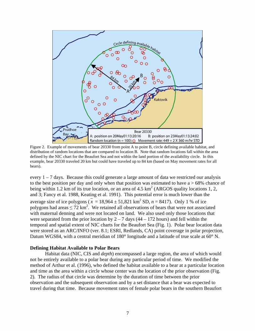
Figure 2. Example of movements of bear 20330 from point A to point B, circle defining available habitat, and distribution of random locations that are compared to location B. Note that random locations fall within the area defined by the NIC chart for the Beaufort Sea and not within the land portion of the availability circle. In this example, bear 20330 traveled 20 km but could have traveled up to 84 km (based on May movement rates for all bears). every 1 – 7 days. Because this could generate a large amount of data we restricted our analysis to the best position per day and only when that position was estimated to have a > 68% chance of being within 1.2 km of its true location, or an area of 4.5 km2 (ARGOS quality locations 1, 2, and 3; Fancy et al. 1988, Keating et al. 1991). This potential error is much lower than the average size of ice polygons ( x = 18,964 ± 51,821 km2 SD, n = 8417). Only 1 % of ice polygons had areas ≤ 72 km2. We retained all observations of bears that were not associated with maternal denning and were not located on land. We also used only those locations that were separated from the prior location by 2 – 7 days (44 – 172 hours) and fell within the temporal and spatial extent of NIC charts for the Beaufort Sea (Fig. 1). Polar bear location data were stored as an ARC/INFO (ver. 8.1; ESRI, Redlands, CA) point coverage in polar projection, Datum WGS84, with a central meridian of 180° longitude and a latitude of true scale at 60° N. Defining Habitat Available to Polar Bears Habitat data (NIC, CIS and depth) encompassed a large region, the area of which would not be entirely available to a polar bear during any particular period of time. We modified the method of Arthur et al. (1996), who defined the habitat available to a bear at a particular location and time as the area within a circle whose center was the location of the prior observation (Fig. 2). The radius of that circle was determine by the duration of time between the prior observation and the subsequent observation and by a set distance that a bear was expected to travel during that time. Because movement rates of female polar bears in the southern Beaufort
7
Sea varies by month (Amstrup et al. 2000), we calculated radii for each unique bear/date observation by the following equation:
radii of available habitat = {a + (b Χ 2)} Χ c;
where a equals the mean hourly movement rate for all bears within each month; b is the standard deviation of the movement rate; and c equals the number of hours between locations (Fig. 2). Sometimes, however, the actual straight-line distance traveled by a bear between observations exceeded the expected distance. In these cases the radius of available habitat was defined as the straight-line distance actually traveled plus 1 meter. Generating Random Locations and Attaching Habitat Variables We compared habitat characteristics of each bear location to a set of up to 100 random points generated with ARC/INFO tools (Fig. 2). These had a minimum spacing of 200 m and were generated in the portion of the availability circle that fell within the NIC chart. Both bear and random locations were merged with NIC and CIS charts, and the ocean depth coverage in order to attach habitat variables. Distance from locations and the nearest edge were calculated. Generating a Resource Selection Function
Estimation of a resource selection function (RSF) followed the methods of McCracken et al. (1998), Arthur et al. (1996) and Cooper and Millspaugh (1999). These methods fit discrete choice models for polar bear site selection and keep the availability of landscape characteristics unique to each polar bear location/date-time combination. That is, points in one polar bear’s circle of available habitat on a particular day were not available for selection by another polar bear, unless the two circles overlapped. The discrete choice model is estimated by maximizing the multinomial logit likelihood (Manly et al. 2002). This was accomplished using the stratified Cox proportional hazards likelihood maximization routine available in the SAS procedure PROC PHREG (SAS Institute 2000). Although PROC PHREG was not designed to fit discrete choice habitat selection functions, Kuhfeld (2000) describes a method by which PROC PHREG can be “tricked” into fitting the appropriate discrete choice likelihood function.
Prior to model building, Pearson’s Correlation Coefficients (r; Conover 1980) were calculated for all main effects for each season. Main effects (Table 1) were excluded from the analysis if |r| ≥ 0.6. Separate models were developed that included one or the other correlated main effect. That is, each member of a pair of correlated main effects was not allowed to enter the same model building procedure. From these, we selected the best model based on how well models appeared to predict the RSF of an independent sample of polar bears locations.
Stepwise model building began with developing a single-term model for each main effect. We set the critical level of covariate entry as α ≤ 0.1 for the adjusted score χ2 (Klein and Moeschberger 1997). The single-term model with the largest significant score χ2 was selected as the start of a forward selection process for model building. We allowed each step of the forward-selection process to add one other term only when the adjusted score χ2 value for that term was α ≤ 0.1. Each forward selection step was preceded by a backward removal step, where the variable with the smallest Wald χ2 value was dropped from the model, provided that α > 0.1. An interaction or quadratic term was not allowed in the model if the main effect involved was not already in the model. If a backward selection step identified a main effect for exclusion, and that main effect was also present in the model in an interaction with another main effect, the main
8
effect was not dropped from the RSF model. The RSF model was considered complete when no other terms could be entered or removed under the constraint of α ≤ 0.1.
As an evaluation of our model building procedure, we compared each model to two other commonly used methods of RSF model building. First, we compared each step in our procedure to the change in the likelihood ratio χ2 each time a covariate was added (Manly et al. 2002). Each coefficient in the final model was also tested to see if it was significantly different from zero. This was done by dividing the coefficient by its standard error, and then comparing the absolute value of this number (z) to a normal distribution. This is the classic Wald t-test, where a value of z > 1.64 indicates a significant difference from zero at α ≤ 0.1 (Manly et al., 2002).
A primary focus of this work was to develop tools that would predict where polar bears may occur. Hence, we were interested in how our seasonal models would perform with real data. To do this we first created a RSF map from the average multi-year habitat values for each season. We then overlaid an independent data set of bear locations on the RSF maps and attached to each bear location its respective RSF value from the seasonal map. The distribution of RSF values assigned to bear locations was then graphically compared to the distribution of RSF values of the map in order to provide an index of the predictive abilities of our models. RESULTS
Between 1 September 1997 and 31 December 2001, 88 PTTs were deployed on 80 polar bears in the Beaufort Sea. A total of 32,105 satellite observations from 77 bears were available for analysis. Following the imposition of temporal and spatial filters, 1780 observations from 53
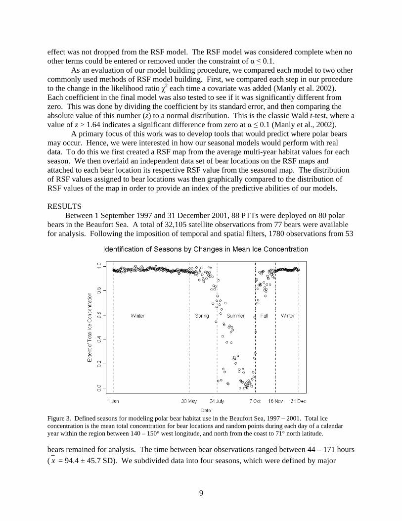
Figure 3. Defined seasons for modeling polar bear habitat use in the Beaufort Sea, 1997 – 2001. Total ice concentration is the mean total concentration for bear locations and random points during each day of a calendar year within the region between 140 – 150° west longitude, and north from the coast to 71° north latitude. bears remained for analysis. The time between bear observations ranged between 44 – 171 hours ( x = 94.4 ± 45.7 SD). We subdivided data into four seasons, which were defined by major
9
seasonal changes in ice concentration near the southern Beaufort Sea coast (Fig. 3). Seasons included spring: 30 May – 23 July; summer: 24 July – 6 October; fall: 7 October – 15 November; and winter: 16 November – 29 May. Seasonal models were unique in their combination of terms (Table 3). Depth appeared in four models and edge appeared in three models. Small changes in depth, and edge resulted in large changes in the relative probability of use (Fig. 4 – 7). Table 3. Seasonal discrete choice models predicting relative probability, w(x), of an adult female polar bear selecting a point in the landscape characterized by x, in the Beaufort Sea, 1997 – 2001. Season Model (standard errors are in parentheses below coefficients) Spring w(x) = exp{-0.0002402(depth) + 0.52481(vastfloe) + 1.67410(totcon)}
(0.0000826) (0.27476) (0.92598) Summer w(x) = exp{-0.01085(edge) + 6.58263(oldice) - 4.93599(oldice2) - 0.0003382(depth)
(0.00440) (1.29720) (1.40941) (0.0000924) + 1.21442(firstyr) + 4.52479(youngice) - 0.29138(edge*youngice)} (0.45996) (1.35200) (0.011078)
Autumn w(x) = exp{-0.00152(depth) – 0.02968(edge) + 3.99265(totcon) (0.0003056) (0.00521) (1.3244) + 0.000000231511(depth2) – 2.70505(totcon2)} (0.000000094957) (1.11305)
Winter w(x) = exp{-0.00170(depth) + 0.000000349299(depth2) + 0.44398(vastfloe) (0.0002075) (0.0000000661291) (0.11599)
+ 1.94584(youngice) – 0.00524(edge) + 0.47312(firstyr)} (0.73993) (0.00244) (0.25120)
Spring
Locations of 36 polar bears entered spring model building. There were a total of 234 actual bear observations and 22,531 random observations ( x = 96.3 ± 5.3 SD random observations per bear observation). High correlations were found between young ice (youngice) and first year ice (firstyr) (r = -0.74, P < 0.0001); old ice (oldice) and youngice (r = 0.74, P < 0.0001); oldice and firstyr (r = -0.92, P < 0.0001); vast floe (vastfloe) and fast ice (fastice) (r = -0.65, P < 0.0001); and vastfloe and big floe (bigfloe) (r = -0.62, P < 0.0001). Four permutations of model building resulted in two spring models. Based on the distribution of an independent sample of polar bear locations, our best spring model started with depth (score χ2 = 5.0378, P = 0.0248). The drop in –2 times log likelihood deviance χ2 between the “no variable” model and the model including depth was 5.097 with 1 df. This is significantly large when compared to a χ2 distribution, indicating that the addition of depth is an improvement to the “no variable” model.
The second forward step created a two-term model with the addition of vastfloe (score χ2 = 5.9091, P = 0.0151). Evidence of model improvement came from a significant drop in the likelihood ratio χ2 between the model with only depth and the model with depth and vastfloe (6.41, 1 df). The entry of totcon (score χ2 = 3.4177, P = 0.0645) followed in the next forward step and was a significant improvement in the model (drop in likelihood ratio χ2: 4.122, 1 df). All three covariates in the final model were significantly different from zero (depth: z = 2.91; vastfloe: z = 1.91; totcon: z = 1.81). A backward step did not identify any covariates for removal from the model. The next forward step identified the interaction of totcon and vastfloe
10
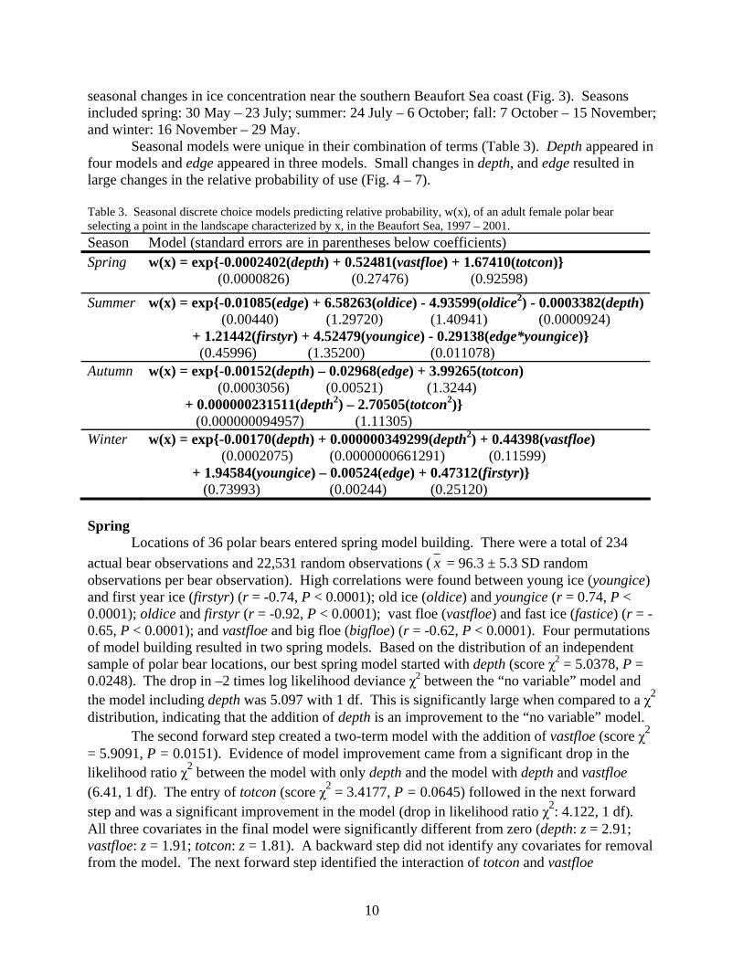
(tot*vfloe). The following backward look, however, dropped tot*vfloe from the model (Wald χ2 = 2.5400, P = 0.1110). When forward steps were continued, the quadratic for vastfloe (vastfloe2) was identified for model inclusion. It too, however, was dropped by the preceding backward look (Wald χ2 = 2.5400, P = 0.1110). Additional forward steps did not identify any other variables that met the α ≤ 0.1 criteria for model entry. The final spring model included the main effect for depth, vastfloe and totcon (Table 3). During spring, polar bears used habitats over water depths between 5 – 3659 m deep, however 50 % of all bear observations occurred in waters ≤ 400 m deep. According to this model, polar bears in the Beaufort Sea select habitat in relatively shallow waters, where ice concentration and the proportion of vast floe is high (Fig. 4).
Total concentration of ice0.0 0.2 0.4 0.6 0.8 1.0 1.2
RS
F
0.0
0.2
0.4
0.6
0.8
1.0
1.2
Spring
Ocean depth (m)0 1000 2000 3000 4000 5000
RS
F
0.30.40.50.60.70.80.91.01.1
Proportion of vast floe0.0 0.2 0.4 0.6 0.8 1.0 1.2
RS
F
0.5
0.6
0.7
0.8
0.9
1.0
1.1
A B
C
Figure 4. Relative probability of selection as a function of variables in the final polar bear sea ice RSF model for spring in the Beaufort Sea, 1999 - 2001. Variables in the final model not in a plot were held at their median values. Summer
Locations of 36 polar bears entered summer model building. There were a total of 256 actual bear observations and 24,531 random observations ( x = 95.8 ± 6.2 SD random observations per bear observation). During summer, there was a significant correlation between oldice and totcon (r = 0.68, P < 0.0001). Model building began with edge (score χ2 = 20.4780, P < 0.0001). The drop in –2 times log likelihood deviance χ2 between the “no variable” model and the model including edge was 23.062 with 1 df. This is significantly large when compared to a χ2 distribution, indicating that the addition of edge is an improvement to the “no variable” model.
11
The next covariate to enter the model was oldice (score χ2 = 21.557, P < 0.0001). The drop in likelihood ratio χ2 between the model with only edge and the model with edge and oldice (21.832, 1df) is significant when compared to a χ2 distribution. The quadratic for oldice (old2) (score χ2 = 15.0429, P = 0.0001) was next to enter the model (drop in likelihood ratio χ2: 14.935, 1 df), then depth (score χ2 = 11.9040, P = 0.0006; drop in likelihood ratio χ2: 11.827, 1 df), then firstyr (score χ2 = 4.7995, P = 0.0285; drop in likelihood ratio χ2: 4.818, 1 df), followed by youngice (score χ2 = 5.8774, P = 0.0153; drop in likelihood ratio χ2: 5.009, 1 df) and the interaction between edge and youngice (edge*youngice) (score χ2 = 7.1407, P = 0.0075; drop in likelihood ratio χ2: 8.583, 1 df). No additional covariates met our criteria for model entry. Our confidence in the summer model was bolstered by significant z-scores for all covariates (edge: z = 2.47; oldice: z = 5.07; old2: z = 3.50; depth: z = 3.66; firstyr: z = 2.64; youngice: z = 3.35; and edge*youngice: z = 2.63).
Ocean depth (m)0 500 1000 1500 2000 2500
RS
F
0.4
0.5
0.6
0.7
0.8
0.9
1.0
1.1
Proportion of area that is old ice0.0 0.2 0.4 0.6 0.8 1.0
0.0
0.2
0.4
0.6
0.8
1.0
1.2
Proportion of area that is first year ice0.0 0.2 0.4 0.6 0.8 1.0
RS
F
0.2
0.4
0.6
0.8
1.0
1.2
SummerA B
C Region outside of predictive capabilities
D
Distance from an ice interface (km)0 20 40 60 80 100
Pro
porti
on o
f are
ath
at is
you
ng ic
e
0.0
0.2
0.4
0.6
0.8
0.2 0.4 0.6 0.8 1.0
DC
Region outside ofpredictive capabilities
RS
F
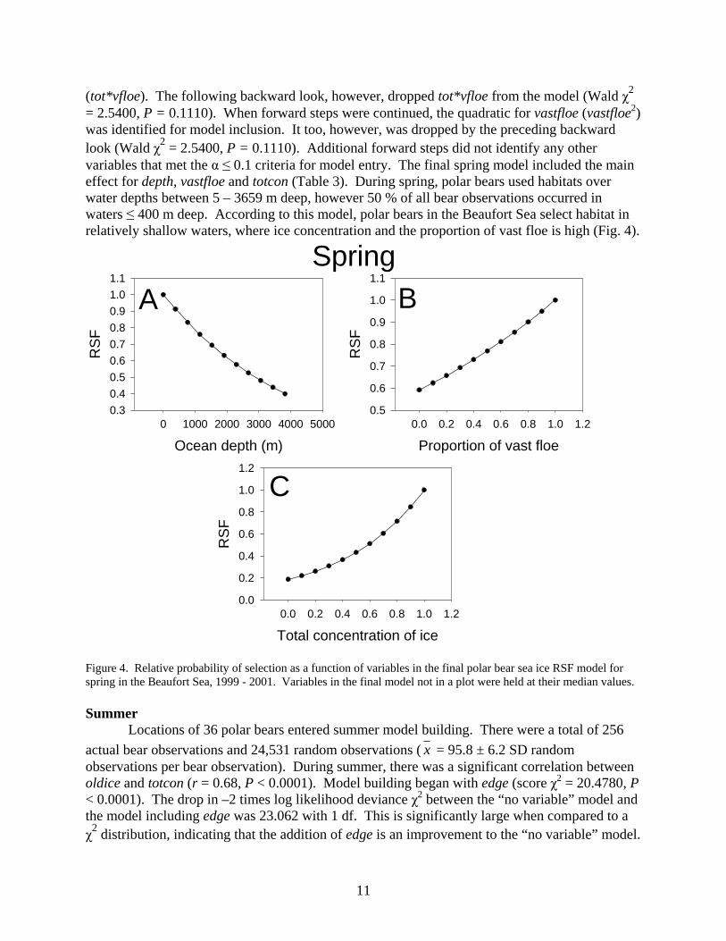
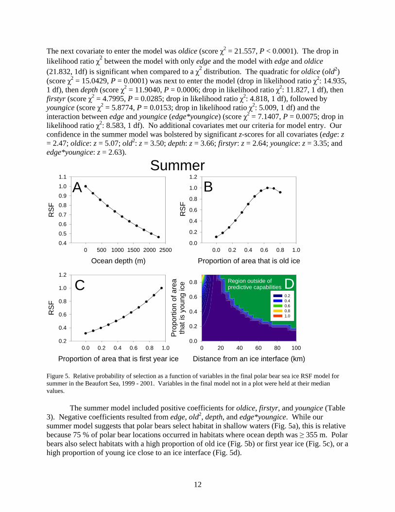
Figure 5. Relative probability of selection as a function of variables in the final polar bear sea ice RSF model for summer in the Beaufort Sea, 1999 - 2001. Variables in the final model not in a plot were held at their median values.
The summer model included positive coefficients for oldice, firstyr, and youngice (Table 3). Negative coefficients resulted from edge, old2, depth, and edge*youngice. While our summer model suggests that polar bears select habitat in shallow waters (Fig. 5a), this is relative because 75 % of polar bear locations occurred in habitats where ocean depth was ≥ 355 m. Polar bears also select habitats with a high proportion of old ice (Fig. 5b) or first year ice (Fig. 5c), or a high proportion of young ice close to an ice interface (Fig. 5d).
12
Autumn
Thirty-nine individual bears entered autumn model building. There were a total of 311 actual bear observations and 29,805 random observations ( x = 95.8 ± 5.4 SD random observations per bear observation). During autumn, there was a significant correlation of oldice with youngice (r = -0.70, P < 0.0001). The highest score χ2 in a single term model resulted with depth (score χ2 = 108.8619, P < 0.0001). The drop in –2 times log likelihood deviance between the “no variable” model and the model including depth was 126.304 with 1 df. This is highly significant when compared to a χ2 distribution, indicating that the addition of depth is an improvement to the “no variable” model. The sequence of covariate entry followed with edge (score χ2 = 41.2362, P < 0.0001). The drop in likelihood ratio χ2 (48.186, 1 df) was significant, indicating model improvement from the model with only depth, to the model including both depth and edge. The next covariate to enter the model was totcon (score χ2 = 7.9508, P = 0.0048; drop in likelihood ratio χ2: 174.49, 1 df). This was followed by the quadratic for depth (depth2) (score χ2 = 6.3139, P = 0.0120; drop in likelihood ratio χ2: 6.42, 1 df), and lastly the quadratic for
Total ice concentration0.0 0.2 0.4 0.6 0.8 1.0 1.2
RS
F
0.0
0.2
0.4
0.6
0.8
1.0
1.2
Ocean depth (m)0 1000 2000 3000 4000 5000
RS
F
0.0
0.2
0.4
0.6
0.8
1.0
1.2
Distance to ice interface (km)0 20 40 60 80 100 120
0.0
0.2
0.4
0.6
0.8
1.0
1.2Autumn
A B
C
RS
F
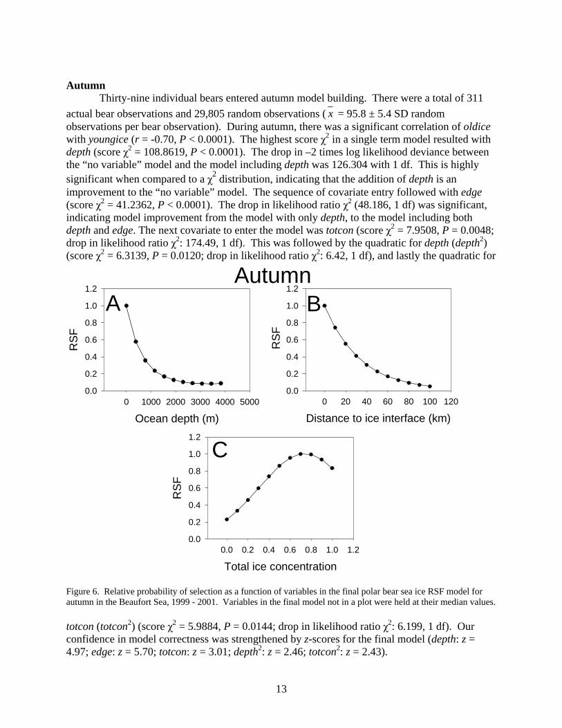
Figure 6. Relative probability of selection as a function of variables in the final polar bear sea ice RSF model for autumn in the Beaufort Sea, 1999 - 2001. Variables in the final model not in a plot were held at their median values. totcon (totcon2) (score χ2 = 5.9884, P = 0.0144; drop in likelihood ratio χ2: 6.199, 1 df). Our confidence in model correctness was strengthened by z-scores for the final model (depth: z = 4.97; edge: z = 5.70; totcon: z = 3.01; depth2: z = 2.46; totcon2: z = 2.43).
13
The autumn model (Table 3) had a positive coefficient for totcon and depth2, and negative coefficients for depth, edge, and totcon2. The quadratic term for depth results in a curvilinear form of the RSF with increasing depth (Fig. 6a). This initially causes a decrease in the RSF with increasing depth. The RSF function, however, approaches an asymptotic pattern when depth was > 1000 m. During autumn, polar bear locations occurred over waters as deep as 3729 m. Of those, 75 % occurred in waters ≤ 189 m deep and 50 % occurred in waters ≤ 30.5 m deep. Our autumn model indicates that polar bears use habitat in relatively shallow water (Fig. 6a) close to an ice interface (Fig. 6b), and with high total ice coverage (Fig. 6c).
Winter
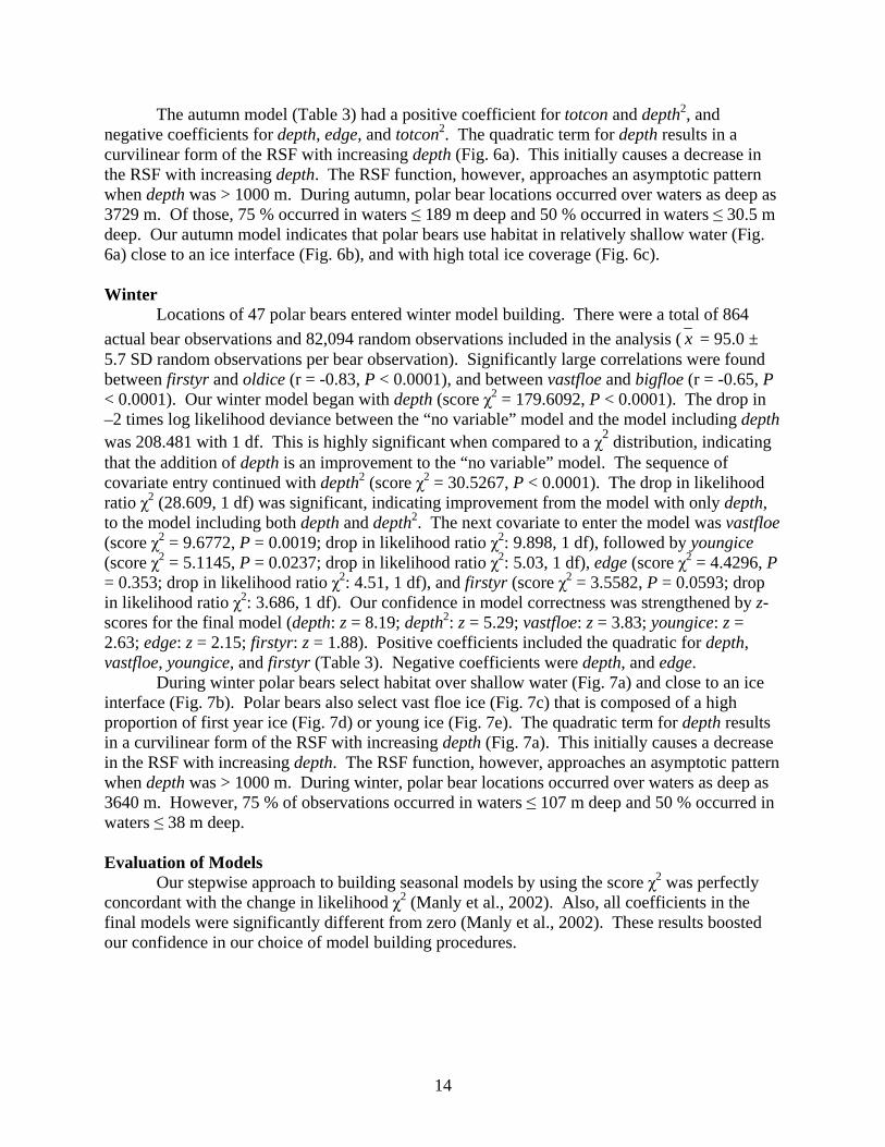
Locations of 47 polar bears entered winter model building. There were a total of 864 actual bear observations and 82,094 random observations included in the analysis ( x = 95.0 ± 5.7 SD random observations per bear observation). Significantly large correlations were found between firstyr and oldice (r = -0.83, P < 0.0001), and between vastfloe and bigfloe (r = -0.65, P < 0.0001). Our winter model began with depth (score χ2 = 179.6092, P < 0.0001). The drop in –2 times log likelihood deviance between the “no variable” model and the model including depth was 208.481 with 1 df. This is highly significant when compared to a χ2 distribution, indicating that the addition of depth is an improvement to the “no variable” model. The sequence of covariate entry continued with depth2 (score χ2 = 30.5267, P < 0.0001). The drop in likelihood ratio χ2 (28.609, 1 df) was significant, indicating improvement from the model with only depth, to the model including both depth and depth2. The next covariate to enter the model was vastfloe (score χ2 = 9.6772, P = 0.0019; drop in likelihood ratio χ2: 9.898, 1 df), followed by youngice (score χ2 = 5.1145, P = 0.0237; drop in likelihood ratio χ2: 5.03, 1 df), edge (score χ2 = 4.4296, P = 0.353; drop in likelihood ratio χ2: 4.51, 1 df), and firstyr (score χ2 = 3.5582, P = 0.0593; drop in likelihood ratio χ2: 3.686, 1 df). Our confidence in model correctness was strengthened by z-scores for the final model (depth: z = 8.19; depth2: z = 5.29; vastfloe: z = 3.83; youngice: z = 2.63; edge: z = 2.15; firstyr: z = 1.88). Positive coefficients included the quadratic for depth, vastfloe, youngice, and firstyr (Table 3). Negative coefficients were depth, and edge.
During winter polar bears select habitat over shallow water (Fig. 7a) and close to an ice interface (Fig. 7b). Polar bears also select vast floe ice (Fig. 7c) that is composed of a high proportion of first year ice (Fig. 7d) or young ice (Fig. 7e). The quadratic term for depth results in a curvilinear form of the RSF with increasing depth (Fig. 7a). This initially causes a decrease in the RSF with increasing depth. The RSF function, however, approaches an asymptotic pattern when depth was > 1000 m. During winter, polar bear locations occurred over waters as deep as 3640 m. However, 75 % of observations occurred in waters ≤ 107 m deep and 50 % occurred in waters ≤ 38 m deep. Evaluation of Models
Our stepwise approach to building seasonal models by using the score χ2 was perfectly concordant with the change in likelihood χ2 (Manly et al., 2002). Also, all coefficients in the final models were significantly different from zero (Manly et al., 2002). These results boosted our confidence in our choice of model building procedures.
14
Winter
E
Ocean depth (m)0 1000 2000 3000 4000 5000
RS
F
0.0
0.2
0.4
0.6
0.8
1.0
1.2
A
Distance to ice interface (km)0 20 40 60 80 100 120
0.5
0.6
0.7
0.8
0.9
1.0
1.1
B
Proportion of vast floe0.0 0.2 0.4 0.6 0.8 1.0 1.2
RS
F
0.6
0.7
0.8
0.9
1.0
1.1
C
Proportion of first year ice0.0 0.2 0.4 0.6 0.8 1.0 1.2
0.6
0.7
0.8
0.9
1.0
1.1
D
Proportion of young ice0.0 0.2 0.4 0.6 0.8 1.0
RS
F
0.0
0.2
0.4
0.6
0.8
1.0
1.2
E
RS
FR
SF
Figure 7. Relative probability of selection as a function of variables in the final polar bear sea ice RSF model for winter in the Beaufort Sea, 1999 - 2001. Variables in the final model not in a plot were held at their median values.
The real test of our models came through a comparison with an independent set of real polar bear location data collected in 2002. These location data were not used in the generation of models. During spring, 81 % of bear locations from 2002 occurred in the highest 30 % of mapped RSF values in the study area (Fig. 8a). During summer (Fig. 8b), the predictive abilities
15
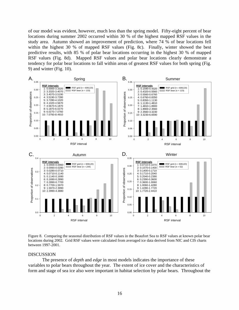
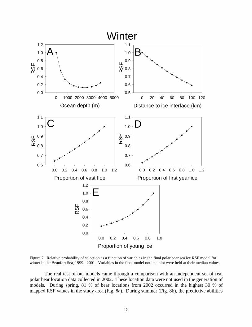
of our model was evident, however, much less than the spring model. Fifty-eight percent of bear locations during summer 2002 occurred within 30 % of the highest mapped RSF values in the study area. Autumn showed an improvement of prediction, where 74 % of bear locations fell within the highest 30 % of mapped RSF values (Fig. 8c). Finally, winter showed the best predictive results, with 85 % of polar bear locations occurring in the highest 30 % of mapped RSF values (Fig. 8d). Mapped RSF values and polar bear locations clearly demonstrate a tendency for polar bear locations to fall within areas of greatest RSF values for both spring (Fig. 9) and winter (Fig. 10).
A. Spring
RSF interval
0 2 4 6 8 10
Pro
porti
on o
f obs
erva
tions
0.00
0.05
0.10
0.15
0.20
0.25
0.30
0.35
RSF grid (n = 606120)RSF bear (n = 133)
RSF intervals 1: 0.0000-3.3320 2: 3.3320-3.4070 3: 3.4070-3.5190 4: 3.5190-3.7280 5: 3.7280-4.1020 6: 4.1020-4.5670 7: 4.5670-5.1870 8: 5.1870-6.0270 9: 6.0270-7.076010: 7.0760-8.4910
B. Summer
RSF interval
0 2 4 6 8 10
Pro
porti
on o
f obs
erva
tions
0.00
0.05
0.10
0.15
0.20
0.25
0.30
0.35
RSF grid (n = 606120)RSF bear (n = 123)
RSF intervals 1: 0.1590-0.4320 2: 0.4320-0.5560 3: 0.5560-0.6760 4: 0.6760-0.8350 5: 0.8350-1.1130 6: 1.1130-1.4810 7: 1.4810-1.8900 8: 1.8900-2.3560 9: 2.3560-3.323010: 3.3230-6.6590
C. Autumn
RSF interval
0 2 4 6 8 10
Pro
porti
on o
f obs
erva
tions
0.0
0.1
0.2
0.3
0.4
RSF grid (n = 606120)RSF bear (n = 244)
RSF intervals 1: 0.0000-0.0060 2: 0.0060-0.0280 3: 0.0280-0.0710 4: 0.0710-0.1140 5: 0.1140-0.1690 6: 0.1690-0.2890 7: 0.2890-0.7700 8: 0.7700-1.5970 9: 1.5970-2.399010: 2.3990-4.3880
D. Winter
RSF interval
0 2 4 6 8 10
Pro
porti
on o
f obs
erva
tions
0.00
0.05
0.10
0.15
0.20
0.25
0.30
0.35
RSF grid (n = 606120)RSF bear (n = 52)
RSF intervals 1: 0.0710-0.1070 2: 0.1070-0.1400 3: 0.1400-0.1710 4: 0.1710-0.2040 5: 0.2040-0.2390 6: 0.2390-0.3600 7: 0.3600-1.0060 8: 1.0060-1.4280 9: 1.4280-1.772010: 1.7720-2.4410
Figure 8. Comparing the seasonal distribution of RSF values in the Beaufort Sea to RSF values at known polar bear locations during 2002. Grid RSF values were calculated from averaged ice data derived from NIC and CIS charts between 1997-2001. DISCUSSION
The presence of depth and edge in most models indicates the importance of these variables to polar bears throughout the year. The extent of ice cover and the characteristics of form and stage of sea ice also were important in habitat selection by polar bears. Throughout the
16
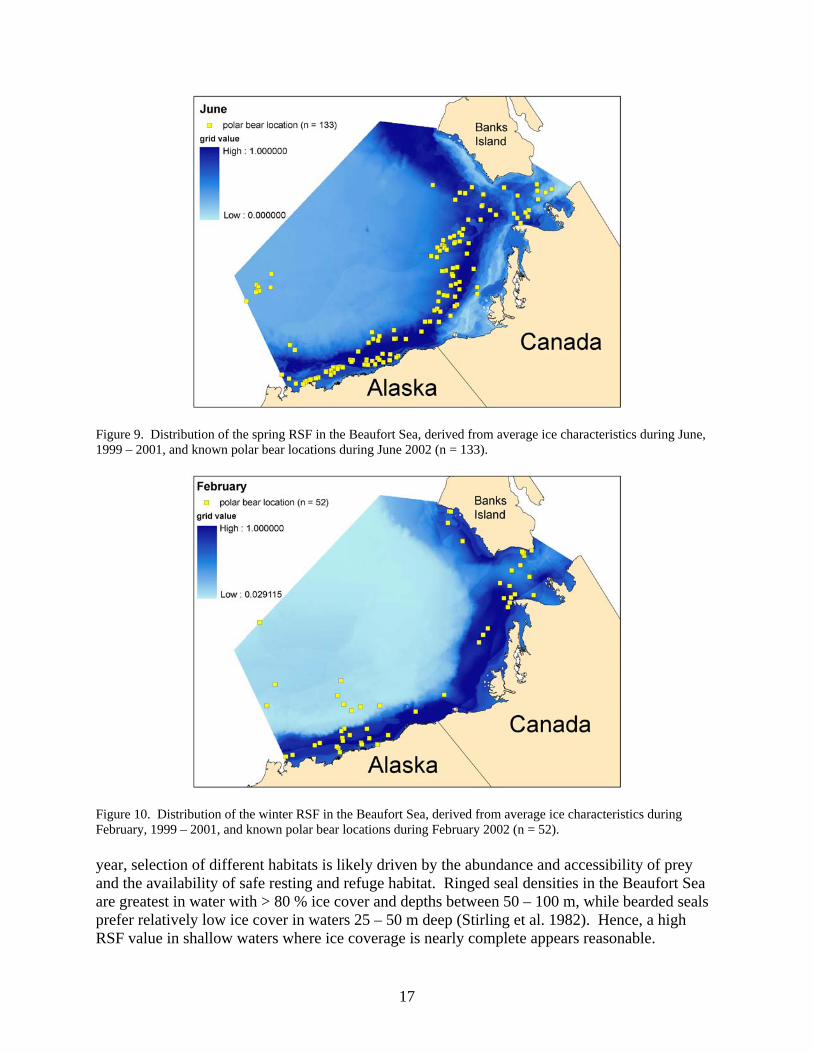
Figure 9. Distribution of the spring RSF in the Beaufort Sea, derived from average ice characteristics during June, 1999 – 2001, and known polar bear locations during June 2002 (n = 133).
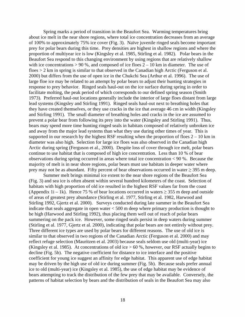
Figure 10. Distribution of the winter RSF in the Beaufort Sea, derived from average ice characteristics during February, 1999 – 2001, and known polar bear locations during February 2002 (n = 52). year, selection of different habitats is likely driven by the abundance and accessibility of prey and the availability of safe resting and refuge habitat. Ringed seal densities in the Beaufort Sea are greatest in water with > 80 % ice cover and depths between 50 – 100 m, while bearded seals prefer relatively low ice cover in waters 25 – 50 m deep (Stirling et al. 1982). Hence, a high RSF value in shallow waters where ice coverage is nearly complete appears reasonable.
17
Spring marks a period of transition in the Beaufort Sea. Warming temperatures bring about ice melt in the near shore regions, where total ice concentration decreases from an average of 100% to approximately 75% ice cover (Fig. 3). Naïve juvenile ringed seals become important prey for polar bears during this time. Prey densities are highest in shallow regions and where the proportion of multiyear ice is low (Kingsley et al. 1985, Stirling et al. 1982). Polar bears in the Beaufort Sea respond to this changing environment by using regions that are relatively shallow with ice concentrations > 90 %, and composed of ice floes 2 – 10 km in diameter. The use of floes > 2 km in spring is similar to that observed in the Canadian high Arctic (Ferguson et al. 2000) but differs from the use of open ice in the Chukchi Sea (Arthur et al. 1996). The use of large floe ice may be related to an attempt by polar bears to adjust their hunting strategies in response to prey behavior. Ringed seals haul-out on the ice surface during spring in order to facilitate molting, the peak period of which corresponds to our defined spring season (Smith 1973). Preferred haul-out locations generally include the interior of large floes distant from large lead systems (Kingsley and Stirling 1991). Ringed seals haul-out next to breathing holes that they have created themselves, or they use cracks in the ice that average 46 cm in width (Kingsley and Stirling 1991). The small diameter of breathing holes and cracks in the ice are assumed to prevent a polar bear from following its prey into the water (Kingsley and Stirling 1991). Thus, bears may spend more time hunting ringed seals in habitats composed of relatively unbroken ice and away from the major lead systems than what they use during other times of year. This is supported in our research by the highest RSF resulting when the proportion of floes 2 – 10 km in diameter was also high. Selection for large ice floes was also observed in the Canadian high Arctic during spring (Ferguson et al., 2000). Despite loss of cover through ice melt, polar bears continue to use habitat that is composed of high ice concentration. Less than 10 % of bear observations during spring occurred in areas where total ice concentration < 90 %. Because the majority of melt is in near shore regions, polar bears must use habitats in deeper water where prey may not be as abundant. Fifty percent of bear observations occurred in water ≥ 395 m deep.
Summer melt brings minimal ice extent to the near shore regions of the Beaufort Sea (Fig. 3) and sea ice is often absent within several hundred kilometers of the coast. Selection of habitats with high proportion of old ice resulted in the highest RSF values far from the coast (Appendix 1i – 1k). Hence 75 % of bear locations occurred in waters ≥ 355 m deep and outside of areas of greatest prey abundance (Stirling et al. 1977, Stirling et al. 1982, Harwood and Stirling 1992, Gjertz et al. 2000). Surveys conducted during late summer in the Beaufort Sea indicate that seals aggregate in open water < 500 m deep where primary production is thought to be high (Harwood and Stirling 1992), thus placing them well out of reach of polar bears summering on the pack ice. However, some ringed seals persist in deep waters during summer (Stirling et al. 1977, Gjertz et al. 2000), indicating that polar bears are not entirely without prey. Three different ice types are used by polar bears for different reasons. The use of old ice is similar to that observed in two regions of the Canadian Arctic (Ferguson et al. 2000) and may reflect refuge selection (Mauritzen et al. 2003) because seals seldom use old (multi-year) ice (Kingsley et al. 1985). At concentrations of old ice > 60 %, however, our RSF actually begins to decline (Fig. 5b). The negative coefficient for distance to ice interface and the positive coefficient for young ice suggest an affinity for edge habitat. This apparent use of edge habitat may be driven by the high use of old ice during summer (Fig. 5b). Because seals prefer annual ice to old (multi-year) ice (Kingsley et al. 1985), the use of edge habitat may be evidence of bears attempting to track the distribution of the few prey that may be available. Conversely, the patterns of habitat selection by bears and the distribution of seals in the Beaufort Sea may also
18
suggest that most polar bears do not feed extensively during summer. This is supported by reports of seasonal activity levels of polar bears. Minimum ice cover and low prey availability resulted in a tendency for polar bears in Canada to decrease their activity in order to conserve energy (Ferguson et al. 2001). Amstrup et al. (2000) showed that polar bears in the Beaufort Sea have their lowest level of movements in September, the time when ice used by polar bears is beyond the preferred habitat of seals.
During autumn, polar bears return to areas of water depths ≤ 189 m, with a high total concentration of ice and close to an ice interface (Fig. 6). In the Beaufort Sea during autumn, near-shore ice concentrations change quickly. Ice concentrations average between 30 – 90 % at the beginning of autumn and increase to ~ 95 % (Fig. 3). Highest RSF values resulted form ice concentrations at approximately 70 – 80 % (Fig. 6c), suggesting that polar bears may select ice of relatively high concentration but interspersed with leads, cracks and other openings. Selection for high ice cover during autumn was observed in two regions in Canada (Ferguson et al. 2000). Selection of habitat near an ice edge may be a response by polar bears to anticipate changes in ice conditions (Ferguson et al. 2000) in a push to get to productive near shore waters where prey abundance is greatest. This is consistent with field observations of polar bears near Prudhoe Bay during autumn (Durner, pers. obs.). In summary, conditions that contribute to a high relative probability of use during autumn include shallow areas with high total ice concentration and when the distance to a polygon edge is < 20 km.
Winter habitat use relative to depth is similar to that observed in all other seasons, with the exception that beyond waters > 1000 m deep, an asymptotic pattern appears (Fig. 7a). Only 9.8 % (86 of 875) of all winter bear observations occurred in habitat where depth was > 1000 m. Habitat use by bears in deep water areas is probably little influenced by additional changes in depth. Winter habitat use shows the greatest tendency of bears to use shallow water areas in the Beaufort Sea. Seventy-five percent of bear observations in winter occurred in waters < 130 m deep. Formation of fast ice and consolidation of off shore ice result in the majority of active ice and leads at shear zones close to and parallel to coastlines (Smith and Rigby 1981). This narrow band of moving ice creates openings that are used by seals. Hence, accessibility of prey is highest there and polar bears respond by selecting active ice (Ferguson et al., 2001). This is reflected in the selection of ice interfaces in our winter model. Thus, polar bears during winter use a relatively small area of the Beaufort Sea where prey abundance is greatest and most accessible. This is concordant with the general pattern of small home range sizes observed for polar bears during most winter months in the Beaufort Sea (Amstrup et al. 2000).
Ferguson et al. (2000) found that polar bears in two regions of the Canadian Arctic select high concentration ice composed of 1st year ice during winter. Multiyear ice generally had a low selection index. Bears also selected landfast ice and large flow ice (> 2000 m) in stable regions in the Arctic Archipelago, but did not select fastice in Baffin Bay (Ferguson et al. 2000). Our winter model also identified vast floe ice (2 – 10 km) as important, with increasing proportions of vast floe resulting in greater selection by polar bears (Fig. 7c). Selection for edge, which was strong in the Beaufort Sea (Fig. 7b), was absent in both regions in the Canada study.
Our models demonstrate the utility of discrete choice models for predicting the seasonal distribution of polar bears in the Beaufort Sea. Both industrial expansion and climate change may impact the sea ice environment that polar bears depend on. Short-term forecasting of polar bear use of sea ice habitat may allow managers to predict effects of industry and oil spills on polar bears and take appropriate remediation. By knowing what ice conditions to expect at a proposed development site we may extrapolate how many polar bears might be affected. Long-
19

term forecasting will allow prediction of sea ice characteristics resulting from climate change. If change can be predicted in total ice concentration, stage and form of ice, and the duration of the ice-free season then we can also predict the resulting distribution of polar bears. The methods and models that we present here are a promising tool that will allow researchers and resource managers to understand the use of sea ice by polar bears in order to make sound management decisions.
20
LITERATURE CITED Amstrup, S. C., G. M. Durner, T. L. McDonald, D. M. Mulcahy, and G. W. Garner. 2001a.
Comparing the movement patterns of satellite-tagged male and female polar bears. Canadian Journal of Zoology 79:2147-2158.
Amstrup, S. C., G. M. Durner, I. Stirling, N. J. Lunn, and F. Messier. 2000. Movements and
distribution of polar bears in the Beaufort Sea. Canadian Journal of Zoology 78:948-966. Amstrup, S. C., and C. Gardner. 1994. Polar bear maternity denning in the Beaufort Sea.
Journal of Wildlife Management 58:1-10. Amstrup, S. C., T. L. McDonald, and I. Stirling. 2001b. Polar bears in the Beaufort Sea: a 30-
year mark-recapture case history. Journal of Agriculture, Biological, and Environmental Statistics 6:221-234.
Amstrup, S. C., I. Stirling, and J. W. Lentfer. 1986. Past and present status of polar bears in
Alaska. Wildlife Society Bulletin 14:241-254. Arthur, S. M., B. F. J. Manly, L. L. McDonald, and G. W. Garner. 1996. Assessing habitat
selection when availability changes. Ecology 77:215-227. Conover, W. J. 1980. Practical nonparametric statistics. Second edition. John Wiley and Sons,
New York, New York, USA. Cooper, A. B., and J. J. Millspaugh. 1999. The application of discrete choice models to wildlife
resource selection studies. Ecology 80:566-575. Drobot, S. D., and J. A. Maslanik. 2002. A practical method for long-range forcasting of ice
severity in the Beaufort Sea. Geophysical Research Letters 29:1-4. Fancy, S. G., L. F. Pank, D. C. Douglas, C. H. Curby, G. W. Garner, S. C. Amstrup, and W. L.
Regelin. 1988. Satellite telemetry: a new tool for wildlife research and management. U. S. Fish and Wildl. Resour. Publ. 172. 54pp.
Ferguson, S. H., M. K. Taylor, E. W. Born, and F. Messier. 1998. Fractals, sea-ice landscape
and spatial patterns of polar bears. Journal of Biogeography 25:1081-1092. Ferguson, S. T., M. K. Taylor, E. W. Born, A. Rosing-Asvid, and F. Messier. 2001. Activity
and movement patterns of polar bears inhabiting consolidated versus active pack ice. Arctic 54:49-54.
Ferguson, S. H., M. K. Taylor, and F. Messier. 2000. Influence of sea ice dynamics on habitat
selection by polar bears. Ecology 81:761-772.
21
Gjertz, I., K. M. Kovacs, C. Lydersen, and Ø. Wiig. 2000. Movements and diving of adult ringed seals (Phoca hispida) in Svalbard. Polar Biology 23:651-656.
Gloersen, P., W. J. Campbell, D. J. Cavalieri, J. C. Comiso, C. L. Parkinson, and H. J. Zwally.
1992. Arctic and Antarctic Sea Ice, 1978 – 1987: Satellite Passive-Microwave Observations and Analysis. Scientific and Technical Information Program, National Aeronautics and Space Administration, Washington, D. C., USA.
Harwood, L. A., and I Stirling. 1992. Distribution of ringed seals in the southeastern Beaufort
Sea during late summer. Canadian Journal of Zoology 70:891-900. Keating, K. A., W. G. Brewster, and C. H. Key. 1991. Satellite telemetry: performance of
animal-tracking systems. Journal of Wildlife Management 55:160-171. Kelly, B. P. 1982. Ringed Seal. Pages 57 – 72 in Selected marine mammals of Alaska. Species
accounts with research and mangement recommendations. Edited by J. W. Lentfer. Marine Mammal Commission, Washington, D. C.
Kingsley, M. C . S., and I. Stirling. 1991. Haul-out behavior of ringed and bearded seals in
relation to defence against surface predators. Canadian Journal of Zoology 69: 1857 – 1861.
Kingsley, M. C. S., I. Stirling, and W. Calvert. 1985. The distribution and abundance of seals in
the Canadian high Arctic, 1980 – 82. Canadian Journal of Fisheries and Aquatic Sciences 42:1189-1210.
Klien, J. P., and M. L. Moeschberger. 1997. Survival analysis, techniques for censored and
truncated data. Springer, New York, New York, USA. Kuhfeld, W. F. 2000. Multinomial Logit, Discrete Choice Modeling: An Introduction to
Designing Choice Experiments, and Collecting, Processing, and Analyzing Choice Data with the SAS System, SAS Technical Report TS-621, SAS Institute, Cary, North Carolina, USA.
Lentfer, J. 1974. Agreement on conservation of polar bears. Polar Record 17:327-330. Lentfer, J. W. 1982. Polar bear. Pages 557 – 566 in J. A. Chapman and G. A. Feldhamer,
editors. Wild Mammals of North America Biology · Management · Economics. The Johns Hopkins University Press, Baltimore, Maryland, USA and London, England.
MANICE. 1994. Manual for Standard Procedures for Observing and Reporting Ice Conditions.
Eighth edition. Ice Services Branch, Atmospheric Environment Service, Ice Centre Environment Canada, Ottawa, Ontario, Canada.
22
Manly, F. J., L.L. McDonald, D. L. Thomas, T. L. McDonald, and W.P. Erickson. 2002. Resource Selection by Animal Statistical Design and Analysis for Field Studies. Second edition. Kluwer Academic Publishers, Dordrecht, The Netherlands.
Mauritzen, M., S. E. Belikov, A. N. Boltunov, A. E. Derocher, E. Hanson, R. A. Ims, Ø. Wiig,
and N. Yoccoz. 2003. Functional responses in polar bear habitat selection. Oikos 100:112-124.
Mauritzen, M., A. E. Derocher, and Ø. Wiig. 2001. Space-use strategies of female polar bears
in a dynamic sea ice habitat. Canadian Journal of Zoology 79:1704-1713. McCracken, M. L., Manly, B. J. F., and Vander Heyden, M. 1998. The use of discrete-choice
models for evaluating resource selection. Journal of Agricultural, Biological, and Environmental Statistics. 3:268-279.
Morison, J., K. Aagaard, and M. Steele. 2000. Recent environmental changes in the Arctic: a
review. Arctic 53:359-371. Neff, J. M. 1990. Composition and fate of petroleum and spill-treating agents in the marine
environment. Pages 1 – 33 in R. Geraci and D. J. St. Aubin, editors. Mammals and Oil Confronting the Risks. Academic Press, Inc. New York, New York, USA.
Nageak, B. P., C. D. Brower, and S. L. Schliebe. 1991. Polar bear management in the southern
Beaufort Sea: an agreement between the Inuvialuit Game Council and North Slope Borough Fish and Game Committee. Transactions of the North American Wildlife Natural Resources Conference. 56:337-343.
Øritsland, N. A., F. R. Engelhardt, F. A. Juck, R. A. Hurst, and P. D. Watts. 1981. Effects of
crude oil on polar bears. Environ. Stud. Rep. No. 24, Northern Affairs Program, Dept. of Indian Affairs and Northern Development, Ottawa, Ontario, Canada.
Parkinson, C. L. 2000. Variability of arctic sea ice: the view from space, an 18-year record.
Arctic 53:341-358. Partington, K., M. Keller, P. Seymour, and C. Bertioa. 1999. Data fusion for use of passive
microwave data in operational sea-ice monitoring. Proceeding, International Geoscience and Remote Sensing Symposium, Hamburg, Germany, 28 June – 2 July.
SAS Institute, Inc. 2000. SAS/STAT Users Guide, SAS Institute, Cary, North Carolina, USA. Smith, M., and B. Rigby. 1981. Distribution of polynyas in the Canadian Arctic. Pages 7 – 28
in I. Stiring and H. Cleator, editors. Polynyas in the Canadian Arctic. Canadian Wildlife Service Occasional Paper, No. 45.
Smith, T. G. 1973. Censusing and estimating the size of ringed seal populations. Fisheries
Research Board of Canada Technical Report No. 427. 17 page + figures.
23
St. Aubin, D. J. 1990. Physiologic and toxic effects on polar bears. Pages 235 – 239 in J. R.
Geraci and D. J. St. Aubin, editors. Sea Mammals and Oil Confronting the Risks. Academic Press, Inc., New York, New York, USA.
Stirling, I. 1990. Polar bears and oil: ecologic perspectives. Pages 223 – 234 in J. R. Geraci and
D. J. St. Aubin, editors. Sea Mammals and Oil Confronting the Risks. Academic Press, Inc., New York, New York, USA.
Stirling, I. 1997. The importance of polynyas, ice edges, and leads to marine mammals and
birds. Journal of Marine Systems10:9-21. Stirling, I., and D. Andriashek. 1992. Terrestrial maternity denning of polar bears in the eastern
Beaufort Sea area. Arctic 45:363-366. Stirling, I., D. Adriashek, and W. Calvert. 1993. Habitat preferences of polar bears in the
western Canadian Arctic in late winter and spring. Polar Record 29:13-24. Stirling, I., W. R. Archibald, and D. DeMaster. 1977. Distribution and abundance of seals in the
eastern Beaufort Sea. Journal of the Fisheries Research Board of Canada 34:976-988. Stirling, I, and A. E. Derocher. 1993. Possible impacts of climatic change on polar bears.
Arctic 46:240-245. Stirling, I., M. Kingsley, and W. Calvert. 1982. The distribution and abundance of seals in the
eastern Beaufort Sea, 1974 – 79. Canadian Wildlife Service Occasional Papers. No. 47. 25 pp.
Stirling, I., N. J. Lunn, and J. Iacozza. 1999. Long-term trends in the population ecology of
polar bears in western Hudson Bay in relation to climatic change. Arctic 52:294-306. Stirling, I., and N. A. Oritsland. 1995. Relationships between estimates of ringed seal (Phoca
hispida) and polar bear (Ursus maritimus) populations in the Canadian Arctic. Canadian Journal of Fisheries and Aquatic Science 52: 2594 – 2612.
Stirling, I., C. Spencer, and D. Andriashek. 1989. Immobilization of polar bears (Ursus
maritimus) with Telazol®. Journal of Wildlife Diseases 25:159-168. Vinnikov, K. Y., A. Robock, R. J. Stouffer, J. E. Walsh, C. L. Parkinson, D. J. Cavalieri, J. F. B.
Mitchell, D. Garrett, and V. F. Zakharov. 1999. Global warming and northern hemisphere sea ice extent. Science 286:1934-1937.
24

APPENDICES
25

PrudhoeBay
Barrow
Appendix 1a. A resource selection function (RSF) for polar bears in the Beaufort Sea during 1 – 31 January (winter). Data were derived from National Ice Center sea ice charts for the Beaufort Sea, Canadian Ice Service ice charts for the West Arctic, and locations of female polar bears equipped with satellite radio collars, during 1999 – 2001.
26

PrudhoeBay
Barrow
Appendix 1b. A resource selection function (RSF) for polar bears in the Beaufort Sea during 1 – 28/29 February (winter). Data were derived from National Ice Center sea ice charts for the Beaufort Sea, Canadian Ice Service ice charts for the West Arctic, and locations of female polar bears equipped with satellite radio collars, during 1999 – 2001.
27
PrudhoeBay
Barrow
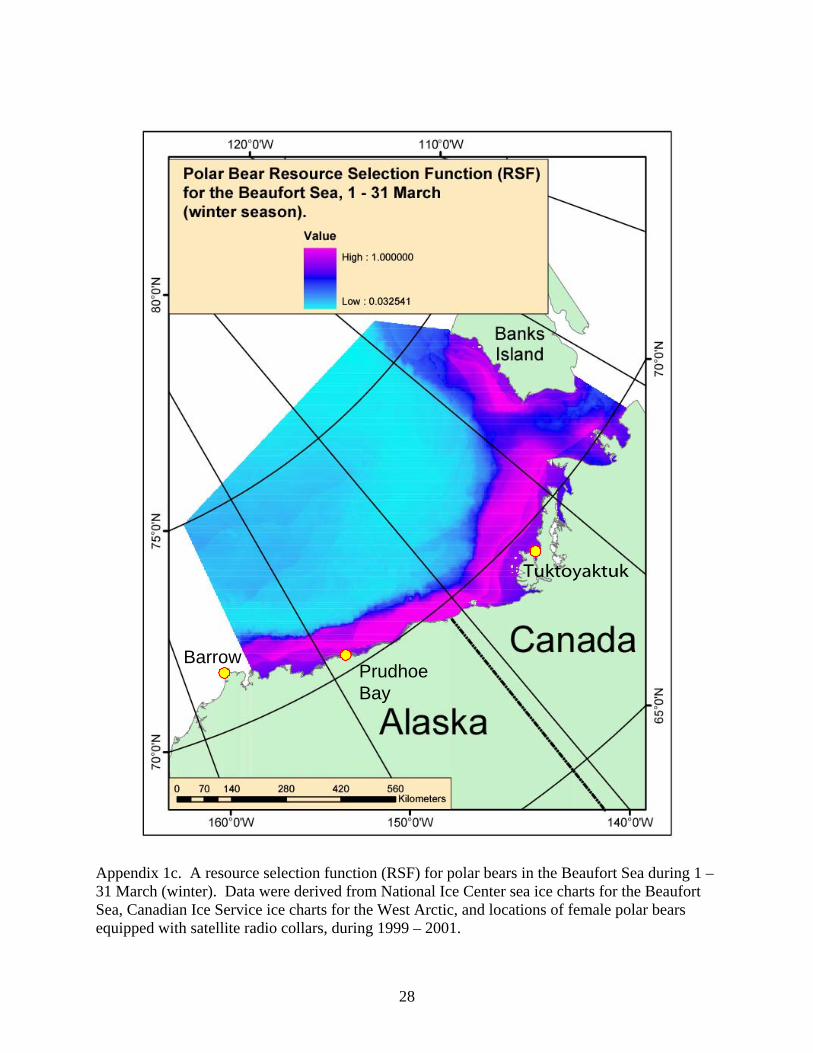
Appendix 1c. A resource selection function (RSF) for polar bears in the Beaufort Sea during 1 – 31 March (winter). Data were derived from National Ice Center sea ice charts for the Beaufort Sea, Canadian Ice Service ice charts for the West Arctic, and locations of female polar bears equipped with satellite radio collars, during 1999 – 2001.
28
PrudhoeBay
Barrow
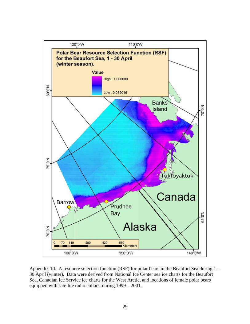
Appendix 1d. A resource selection function (RSF) for polar bears in the Beaufort Sea during 1 – 30 April (winter). Data were derived from National Ice Center sea ice charts for the Beaufort Sea, Canadian Ice Service ice charts for the West Arctic, and locations of female polar bears equipped with satellite radio collars, during 1999 – 2001.
29
PrudhoeBay
Barrow
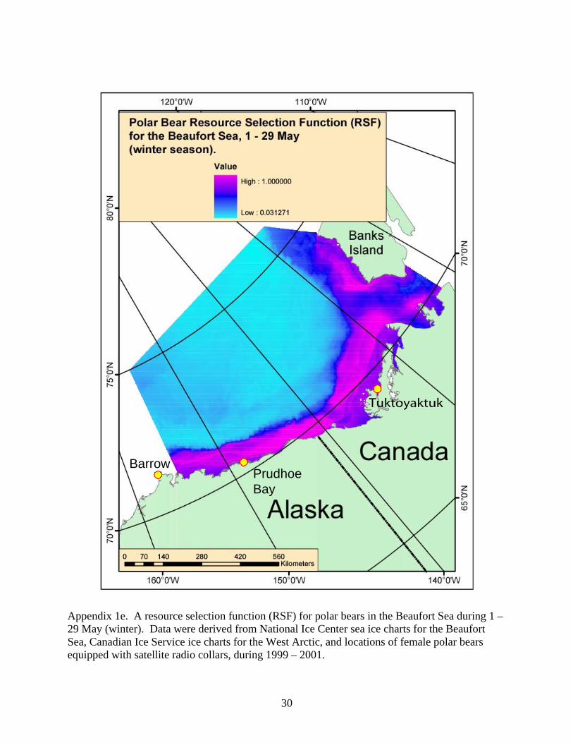
Appendix 1e. A resource selection function (RSF) for polar bears in the Beaufort Sea during 1 – 29 May (winter). Data were derived from National Ice Center sea ice charts for the Beaufort Sea, Canadian Ice Service ice charts for the West Arctic, and locations of female polar bears equipped with satellite radio collars, during 1999 – 2001.
30
PrudhoeBay
Barrow
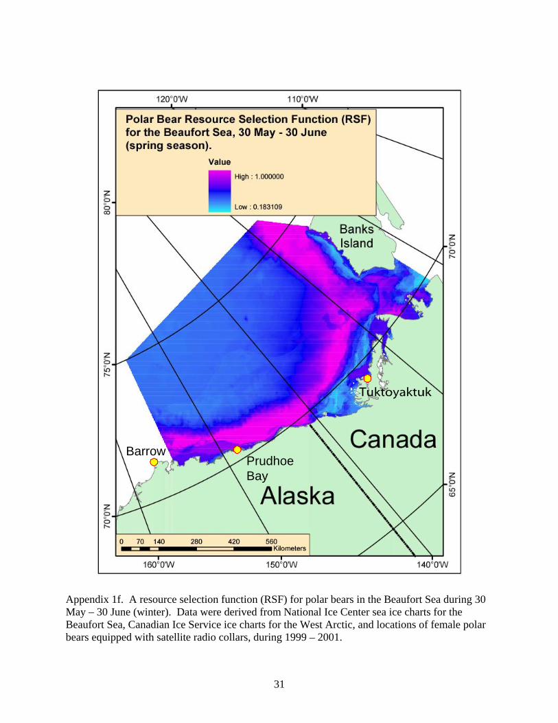
Appendix 1f. A resource selection function (RSF) for polar bears in the Beaufort Sea during 30 May – 30 June (winter). Data were derived from National Ice Center sea ice charts for the Beaufort Sea, Canadian Ice Service ice charts for the West Arctic, and locations of female polar bears equipped with satellite radio collars, during 1999 – 2001.
31
PrudhoeBay
Barrow
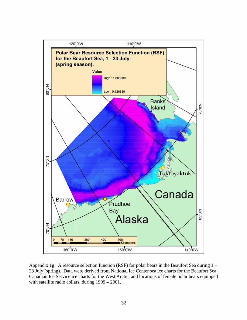
Appendix 1g. A resource selection function (RSF) for polar bears in the Beaufort Sea during 1 – 23 July (spring). Data were derived from National Ice Center sea ice charts for the Beaufort Sea, Canadian Ice Service ice charts for the West Arctic, and locations of female polar bears equipped with satellite radio collars, during 1999 – 2001.
32
PrudhoeBay
Barrow
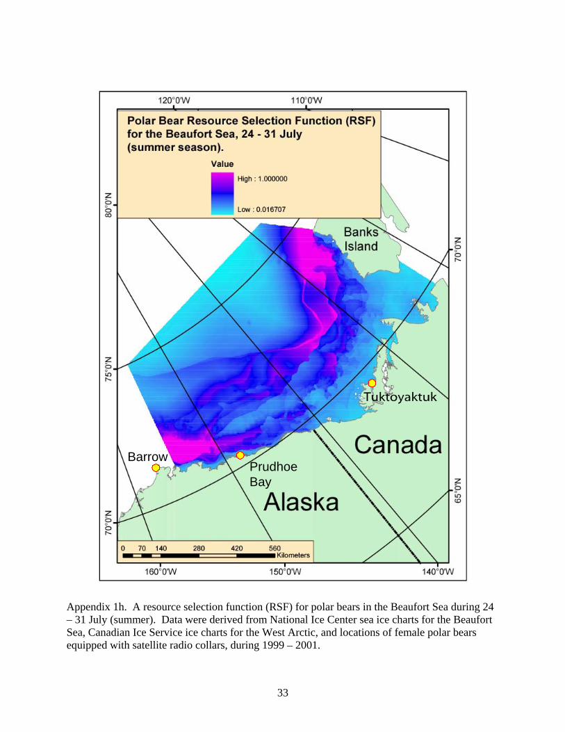
Appendix 1h. A resource selection function (RSF) for polar bears in the Beaufort Sea during 24 – 31 July (summer). Data were derived from National Ice Center sea ice charts for the Beaufort Sea, Canadian Ice Service ice charts for the West Arctic, and locations of female polar bears equipped with satellite radio collars, during 1999 – 2001.
33
PrudhoeBay
Barrow
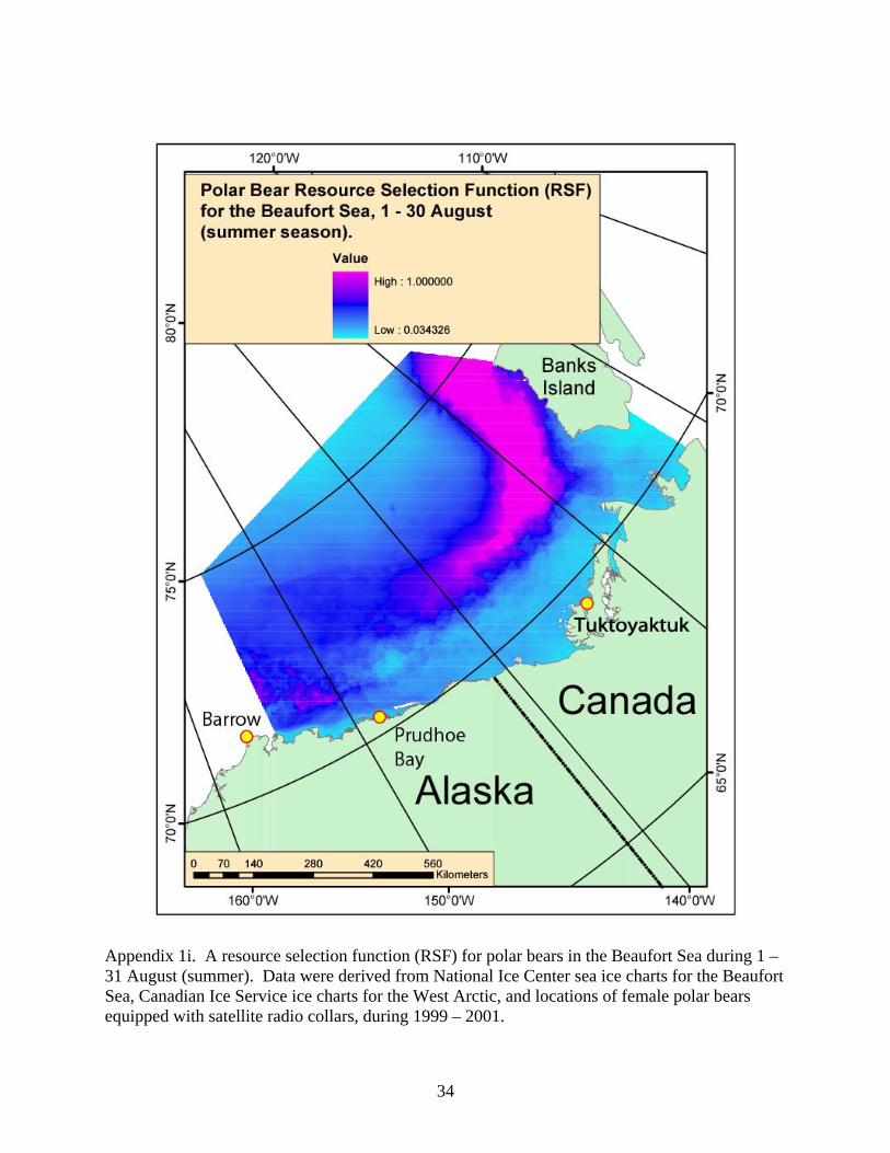
Appendix 1i. A resource selection function (RSF) for polar bears in the Beaufort Sea during 1 – 31 August (summer). Data were derived from National Ice Center sea ice charts for the Beaufort Sea, Canadian Ice Service ice charts for the West Arctic, and locations of female polar bears equipped with satellite radio collars, during 1999 – 2001.
34
PrudhoeBay
Barrow
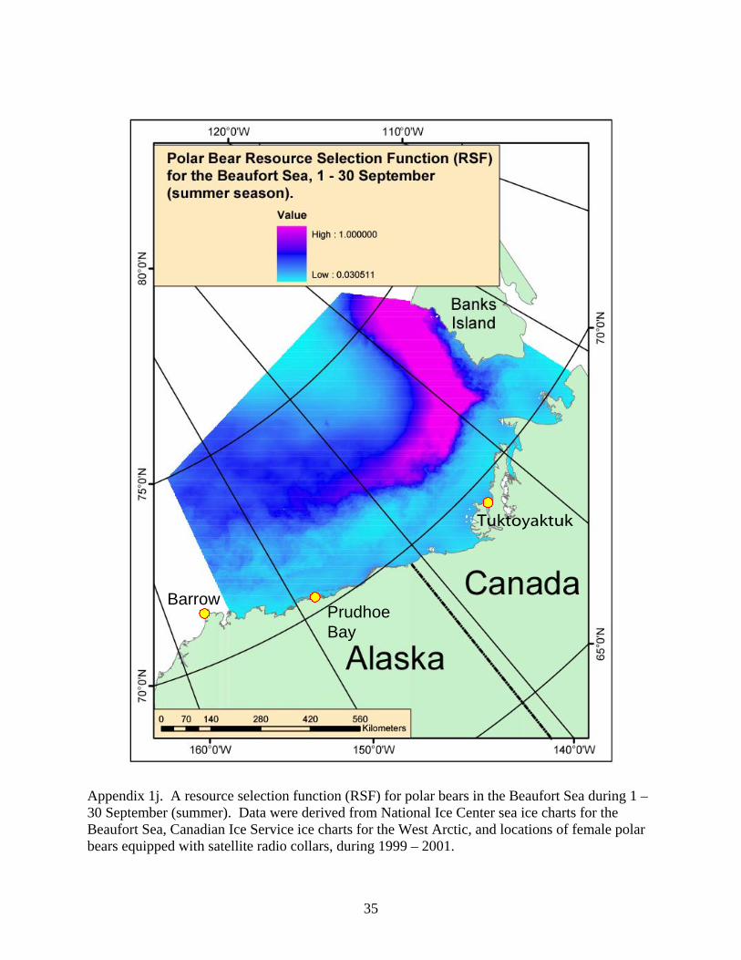
Appendix 1j. A resource selection function (RSF) for polar bears in the Beaufort Sea during 1 – 30 September (summer). Data were derived from National Ice Center sea ice charts for the Beaufort Sea, Canadian Ice Service ice charts for the West Arctic, and locations of female polar bears equipped with satellite radio collars, during 1999 – 2001.
35
PrudhoeBay
Barrow
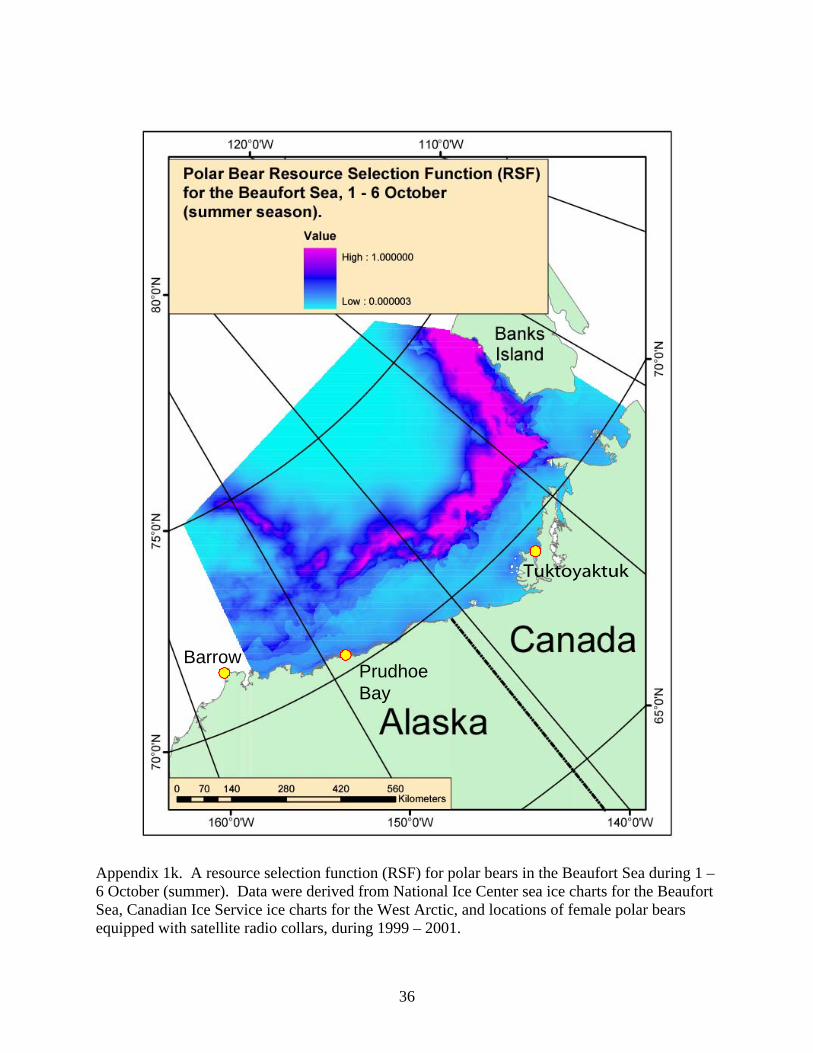
Appendix 1k. A resource selection function (RSF) for polar bears in the Beaufort Sea during 1 – 6 October (summer). Data were derived from National Ice Center sea ice charts for the Beaufort Sea, Canadian Ice Service ice charts for the West Arctic, and locations of female polar bears equipped with satellite radio collars, during 1999 – 2001.
36
PrudhoeBay
Barrow
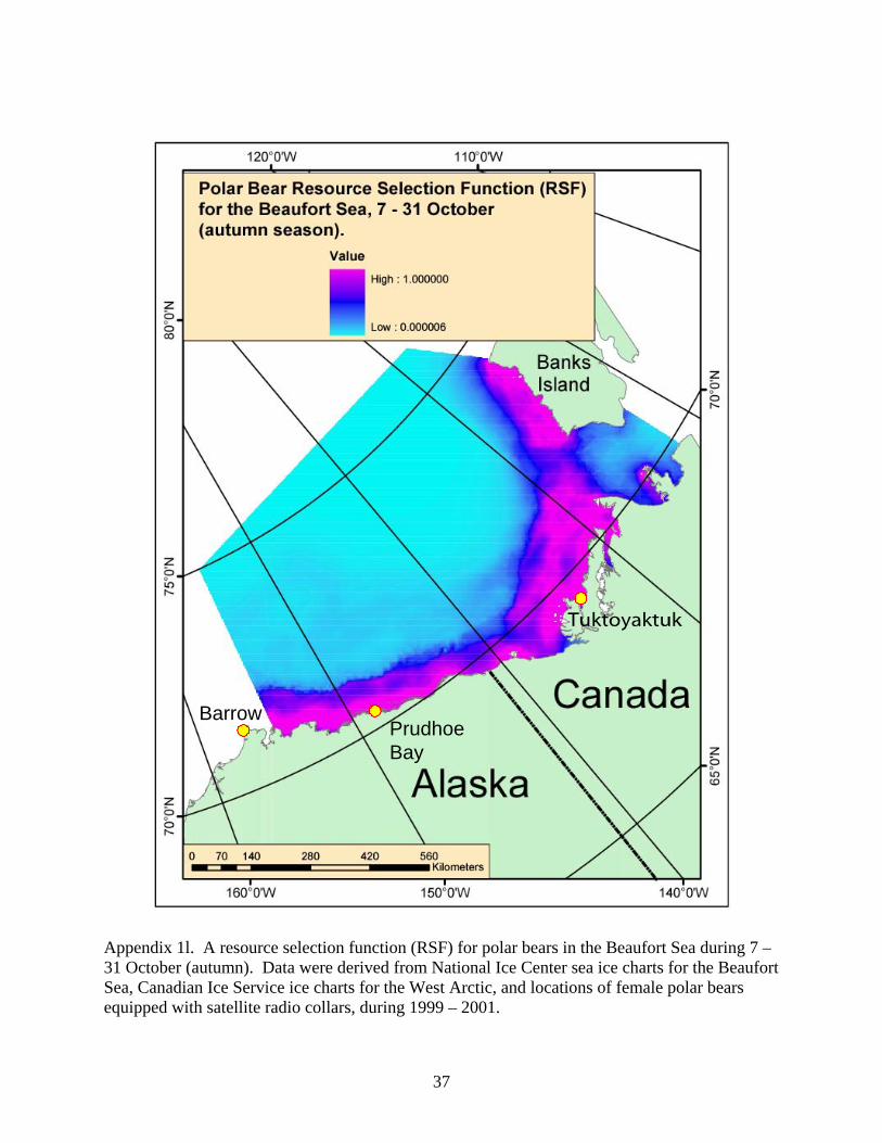
Appendix 1l. A resource selection function (RSF) for polar bears in the Beaufort Sea during 7 – 31 October (autumn). Data were derived from National Ice Center sea ice charts for the Beaufort Sea, Canadian Ice Service ice charts for the West Arctic, and locations of female polar bears equipped with satellite radio collars, during 1999 – 2001.
37
PrudhoeBay
Barrow
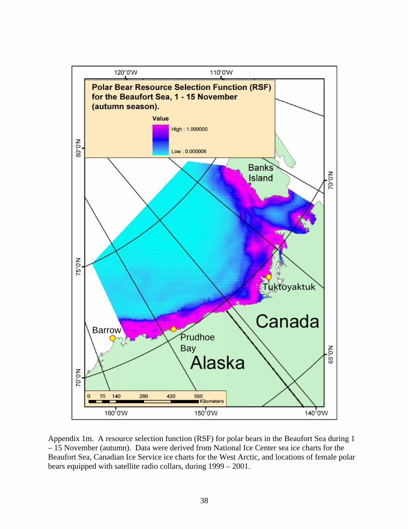
Appendix 1m. A resource selection function (RSF) for polar bears in the Beaufort Sea during 1 – 15 November (autumn). Data were derived from National Ice Center sea ice charts for the Beaufort Sea, Canadian Ice Service ice charts for the West Arctic, and locations of female polar bears equipped with satellite radio collars, during 1999 – 2001.
38
PrudhoeBay
Barrow
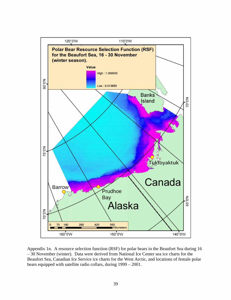
Appendix 1n. A resource selection function (RSF) for polar bears in the Beaufort Sea during 16 – 30 November (winter). Data were derived from National Ice Center sea ice charts for the Beaufort Sea, Canadian Ice Service ice charts for the West Arctic, and locations of female polar bears equipped with satellite radio collars, during 1999 – 2001.
39
PrudhoeBay
Barrow
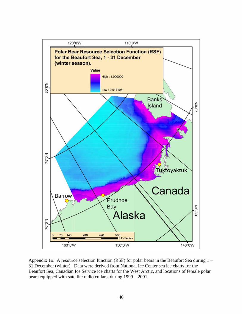
Appendix 1o. A resource selection function (RSF) for polar bears in the Beaufort Sea during 1 – 31 December (winter). Data were derived from National Ice Center sea ice charts for the Beaufort Sea, Canadian Ice Service ice charts for the West Arctic, and locations of female polar bears equipped with satellite radio collars, during 1999 – 2001.
40

Appendix 2. List of project publications, reports, and presentations Durner, G. M., S.C. Amstrup, R. Neilson, and T. McDonald. In press. Using discrete choice
modeling to create resource selection functions for female polar bears in the Beaufort Sea. 1st International Conference on Resource Selection by Animals. 13-15 January 2003, University of Wyoming, Laramie, WY. Proceedings from presentation.
41