Journal of Computer Sciences 1 (1): 47-62, 2005 ISSN 1549-3636 © Science Publications, 2005

47

The Use of Neural Networks in Real-time Face Detection

Kevin Curran, Xuelong Li and Neil Mc Caughley Internet Technologies Research Group, University of Ulster

Magee Campus, Northland Road, Northern Ireland, BT48 7JL, UK

Abstract: As continual research is being conducted in the area of computer vision, one of the most practical applications under vigorous development is in the construction of a robust real-time face detection system. Successfully constructing a real-time face detection system not only implies a system capable of analyzing video streams, but also naturally leads onto the solution to the problems of extremely constraint testing environments. Analyzing a video sequence is the current challenge since faces are constantly in dynamic motion, presenting many different possible rotational and illumination conditions. While solutions to the task of face detection have been presented, detection performances of many systems are heavily dependent upon a strictly constrained environment. The problem of detecting faces under gross variations remains largely uncovered. This study presents a real-time face detection system which uses an image based neural network to detect images. Key words: Face Detection System, Real-Time, Neural Network, Images

INTRODUCTION

The face is the most distinctive and widely used key to a person’s identity. The area of Face detection has attracted considerable attention in the advancement of human-machine interaction as it provides a natural and efficient way to communicate between humans and machines. The problem of detecting the faces and facial parts in image sequences has become a popular area of research due to emerging applications in intelligent human-computer interface, surveillance systems, content-based image retrieval, video conferencing, financial transaction, forensic applications, pedestrian detection, image database management system and so on. Face detection is essentially localising and extracting a face region from the background. This may seem like an easy task but the human face is a dynamic object and has a high degree of variability in its appearance, which makes face detection a difficult problem in computer vision. Consider the pictures in Fig. 1 these are typical images that could be used in face classification research. They have no background and are all front facing. Any face detection program should have no trouble in detecting these. A wide variety techniques have been developed ranging from simple edge-based algorithms to composite high level approaches using advanced pattern recognition methods [1, 2, 3, 4, 5]. Face detection can be established by a feature-based method and an image-based method. Feature Based Method to Face Detection: This area contains techniques that are classified as low-level analysis. These are methods that that deal with the segmentation of visual features using pixel properties such as gray-scale and colour. The features that these

low-level methods detect can be ambiguous, but these methods are easy to implement and fast. Another area of techniques called feature analysis, where face detection is based upon facial features using information of face geometry. Through feature analysis, feature ambiguities are reduced and locations of the face and facial features are determined. The last group involves the use of active shape models. These have been developed for the purpose of complex and non-rigid feature extraction such as eyes and lip tracking. Low-level Analysis Edges: This is the most primitive feature in face detection applications. The earliest of this work was done by [6]. Most of the work was based on basic line drawings of faces from photographs, aiming to locate facial features. Further work was carried out by [4] whose work led to tracing a human head outline. This was the basis of the detection program, where the next step was feature analysis to determine if the shape detected was indeed a human face shape. Edge detection essentially locates major outlines in the image (the threshold can be set to detect predominant lines or indeed all lines). It then assigns each pixel on the line with a binary digit to set it out from the back ground. Many types of edge operators exist. They all operate on the same premise and give similar results. Fig. 3 and 4 show some of the edge routines applied to Fig. 2. In an edge-detection based approach to face-detection, the edges (after identification) need to be labelled and matched to a face model in order to verify correct detections. Features have to be located and identified such as eyes, hairline or jaw line. If these all seem to be in ratio and in place a face is detected. This method is accurate in images with no complex backgrounds and

J. Comp.,Sci., 1 (1): 47-62, 2005

48

Fig. 1: Images that could be used for Face Classification

Fig. 2: Original Image Fig. 3: Sobel Edge Filtering Fig. 4: Canny Edge Filtering Average Lengths (Times the Reference Length) of Facial Features

Head Height Eye Separation Eye to Nose Eye to Mouth Average Length 1.972 0.516 0.303 0.556

Fig. 5: Table showing De Silva’s et al [17] Findings

the face needs to be in clear view facing front. These limitations sometimes restrict edge detection implemented as a pre-processing tool to identify face shapes and then these figures are handed over to a pattern based system for more accurate detection process. Colour Segmentation: The detection of skin colour in colour images is a very popular and useful technique for face detection. This section explains an approach for determining the skin coloured parts of an image. Many Techniques have reported locating skin colour regions in an image [1, 2, 7, 8]. While the input colour image is typically in the RGB format, the RGB model is not used in the detection process. It is well known that the RGB colour model is not a reliable model for detecting skin colour. This is because RGB components are subject to luminance change, this means face detection may fail if the lighting condition changes from image to image. The technique usually uses colour components in the colour space, such as HSV or YCbCr [2]. The colour model that we use is the YIQ model, a universal colour space used for colour television transmission.

Feature Analysis Feature Searching: Feature searching works on the premise that it exclusively looks for prominent facial features in the image. After this main detection less prominent features are searched for using standard measurements of facial geometry. A pair of eyes is the most commonly applied reference feature [8, 9,10]. Other features include the top of the head and the main face axis. This method is often combined with edge detection where the edge densities are detected from a top-down approach starting from the top of the head. These are measured and after distinguishing a reference measurement. These measurements are plotted against the average lengths of facial measurements (which is found by measuring a set of varying face images held on a database). Fig. 5 shows a table showing the average measurements in respect to reference length obtained from the modelling of 42 frontal faces in a database. This method does not rely on skin colour and so manages to detect various races. This method is also restricted to frontal face images with a plain background and it need a clear forehead not hidden by

J. Comp.,Sci., 1 (1): 47-62, 2005

49

hair to ensure detection. If facial hair, earrings and eyewear are worn on the face it fails to detect the face. Active Shape Models Snakes: Snakes (or Active Contours) were first introduced by [11]. They are commonly used to locate a head boundary. This is done by firstly initialising the snake at the proximity around the head boundary. The snake locks onto the nearby edges and subsequently assumes the shape of the head. The snakes path is determined by minimising an energy function, Esnake, denoted as Esnake = Einternal + Eexternal Where Einternal, Eexternal are the internal and external energy functions. The internal energy defines the snake’s natural evolution and external counteracts the internal energy to enable the contours to deviate from the natural evolution and assume the shape of nearby features – ideally the head boundary. The appropriate energy terms have to be considered. Elastic energy is used commonly as internal energy – this can give the snake the elastic-band characteristic that causes the snake’s evolution (by shrinking and expanding). The external energy requirement can include a skin colour function which attracts the skin colour function to the face region. Snakes are well equipped to detect feature boundaries but it still has its problems. The contours often get trapped on false image features causing the program to crash. Snakes also try to keep to the minimum curvature and this can lead to problems as some face shapes may not be completely convex and thus will return false results. Point Distributed Models: This method takes the statistical information of the shape given in an image and compares it to a pre-defined training set to determine whether the shape is a head (or indeed a head shape) [12]. The point distributed model created by the program is put into a set of points which are labelled. Variations of these points are first determined by using the training set that includes objects of different sizes and poses. Using principal component analysis, variations of the features in a training set are constructed as a linear flexible model. The model comprises the mean of all the features in the sets and the principle modes of variation for each point where x represents a point on the point distributed model, x is the mean feature in the training set for that point, P = [p1 p2 … pt] is the matrix of the t most significant variation vectors of the covariance of deviations, and v is the weight vector for each mode. x = x + Pv Face point distribution models were first developed by Lanitis et al. as a flexible model. This model defines a global model for a face which includes facial features such as eye-brows, the nose and eyes. Using 152 manually planted control points (x) and 160 training face images, the face point distribution model is

obtained. For comparison the mean shape model x is placed on top (or near) the area being tested. The labels of each image are then compared. During the comparison the corresponding points are only allowed to differ in a way that is consistent with the training set data. The global characteristic of the model means that all features can be detected simultaneously so this means that the need for feature searching is removed, cutting down pre-processing time. Another advantage of this technique is that it can detect a face even if a feature is missing – hidden or removed. This is because other feature comparisons can still detect the face. This technique needs to be further developed to detect multiple faces in images. Face Detection Using Colour Segmentation: Our research uses a combination of techniques to identify a face. This is intended to increase accuracy. We firstly use skin colour segmentation to detect a possible face region in an image. We then put this region through a more complex pattern recognition program to identify a face. The image is tested in the YIQ space to test each pixel to determine and to classify if it’s either skin or non-skin [1]. A lookup table is employed to classify the “skinness” of each pixel, where each colour is tested to see if it lies in the range of skin colour and be associated a binary value of one if it is and zero if not. A bounded box is needed to determine the range and location of the values of ones. The purpose of the colour segmentation is to reduce the search space of the subsequent techniques, so it is important to determine as tight a box as possible without cutting off the face. After the colour image has been mapped into a binary image of ones and zeros representing skin and non-skin regions. It is common during the colour segmentation to return values that are closely skin but non-skin, or other skin-like coloured regions that is not part of the face or the body. These noisy erroneous values are generally isolated pixels or group of pixels that are dramatically smaller than the total face regions. Inclusion of these noisy pixels would result in a box that is much larger than intended and defeat the purpose of the segmentation. Further morphological refinements are applied to the binary output in order to reduce some of the effects of these noisy pixels. Since these spurious errors are generally much smaller than the face region itself, morphological techniques such as erosion, filtering and closing are good tools to use to eliminate these pixels. Image Based Approach to Face Detection: The image based approach to face detection is plagued by the unpredictability of image environmental conditions and unpredictable face appearances. The image based approach is usually limited to detecting one face in a non complex background with ideal conditions. There is a need for techniques that can detect multiple faces with complex backgrounds. The pattern recognition

J. Comp.,Sci., 1 (1): 47-62, 2005

50

area of face detection was developed for these reasons. This technique works on the idea that the face is recognised by comparing an image to examples of face patterns. This eliminates the use of face knowledge as the detection technique. This means inaccurate or uncompleted data from facial images can still be detected as a face. The approach here is to classify an area as either face or non-face, so a set of face and non-face prototypes must be trained to fit these patterns. These form a 2D intensity array (thus the name image based) to be compared with a 2D array taken from the input image test area. This then decides whether the face falls into a face or non-face type. In the following sections, we present some of the complex techniques that use a feature based approach. These are Eigenfaces, Neural Networks and Support Vector Machines. EigenFaces: In the late 1980s, [13] developed a technique using principal component analysis to efficiently represent human faces. Given an ensemble of different face images, the technique first finds the principal components of the distribution of faces, expressed in terms of eigenvectors (taken from a 2D image matrix). Each individual face in the face set can then be approximated by a linear combination of the largest eigenvectors, more commonly referred to as eigenfaces, using appropriate weights. The eigenfaces are determined by performing a principal component analysis on a set of example images with central faces of the same size. In addition the existence of a face in a given image can be determined. By moving a window covering a sub image over the entire image faces can be located within the entire image. A pre compiled set of photographs comprise the training set, and it is this training set that the eigenfaces are extracted from. The photographs in the training set are mapped to another set which are the eigenfaces. As with any other mapping in mathematics, we can now think of the data (the photographs and the eigenfaces) as existing in two domains. The photographs in the training set are one of these domains, and the eigenfaces comprise the second domain that is often referred to as the face space. Fig. 6 shows an example of eigenfaces that could be generated to make up the face space. The eigenfaces that comprise the face space are added together with appropriate weights to re-compose one of the photographs in the training set. It is through the analysis of these weights that face detection can be realized. A training set of 100 to 150 images is enough to generate appropriate eigenfaces. Neural Networks: Neural Networks have become a popular technique for pattern recognition face detection [14,15, 16]. They contain a stage made up of multilayer perceptrons. Other techniques are also applied to add to the complexity of its process.

Modular architectures, committee–ensemble classification, complex learning algorithms, auto associative and compression networks, and networks evolved or pruned with genetic algorithms are all examples of the widespread use of neural networks in pattern recognition. The first neural approaches were based on Multi-layer perceptrons which gave promising results with fairly simple datasets. The first advanced neural approach which reported results on a large, difficult dataset was by [16]. Rowley’s system incorporates face knowledge in a retinally connected neural network shown in Fig. 7. The neural network is designed to look at windows of 20 x 20 pixels (thus 400 input units). There is one hidden layer with 26 units, where 4 units look at 10 x 10 pixel sub regions, 16 look at 5 x 5 sub regions, and 6 look at 20 x 5 pixels overlapping horizontal stripes. The input window is pre-processed through lighting correction (a best fit linear function is subtracted) and histogram equalization. A problem that arises with window scanning techniques is overlapping detections. [17] deals with this problem through two heuristics: 1. Thresholding: the number of detections in a

small region surrounding the current location is counted, and if it is above a certain threshold, a face is present at this location.

2. Overlap elimination: when a region is classified

as a face according to thresholding, then overlapping detections are likely to be false positives and thus are rejected.

During training, the target for a face-image is the reconstruction of the image itself, while for nonface examples; the target is set to the mean of the n nearest neighbours of face images. A training algorithm based on the bootstrap algorithm of Sung and Poggio [7] was employed (and also a similar pre-processing method consisting of histogram equalization and smoothing). The system is trained with a simple learning rule which promotes and demotes weights in cases of misclassification. Similar to the Eigenface method, [18] use the bootstrap method of Sung and Poggio for generating training samples and pre-process all images with histogram equalization. The training set outlined in Error! Reference source not found. can also be used in this training circumstance. Support Vector Machines: Support vector machine is a patter classification algorithm developed by V. Vapnik and his team at AT &T Bell Labs [19, 20]. While most machine learning based classification techniques are based on the idea of minimising the error in training data ( empirical risk ) SVM’s operate on another induction principle , called

J. Comp.,Sci., 1 (1): 47-62, 2005

51

Fig. 6: Possible Eigenface Images

Fig. 7: The system of Rowley [16] structural risk minimization, which minimizes an upper bound on the generalization error. Training is performed with a boot-strap learning algorithm [21]. Generating a training set for the SVM is a challenging task because of the difficulty in placing “characteristic” non-face images in the training set. To get a representative sample of face images is not much of a

problem; however, to choose the right combination of non-face images from the immensely large set of such images is a complicated task. For this purpose, after each training session, non-faces incorrectly detected as faces are placed in the training set for the next session. This “bootstrap” method overcomes the problem of using a huge set of non-face images in the training set,

J. Comp.,Sci., 1 (1): 47-62, 2005

52

many of which may not influence the training [7]. To test the image for faces, possible face regions detected by another technique (say, colour segmentation) will only be tested to avoid exhaustive scanning. In order to explain SVM process consider data points of the form {(xi,yi)}i=1..N. We wish to determine among the infinite such points in an N-dimensional space which of two classes of such points does a given point belong to. If the two classes are linearly separable, we need to determine a hyper-plane that separates these two classes in space. However, if the classes are not clearly separable, then our objective would be to minimize the smallest generalization error. Intuitively, a good choice is the hyper-plane that leaves the maximum margin between the two classes (margin being defined as the sum of the distances of the hyper-plane from the closest points of the two classes), and minimizes the misclassification errors. The same data used to train a neural network can be trained here. The learning time for SVM algorithms are significantly smaller than that for the neural network. Back propagation of a neural network takes more time than the required training time of a SVM training period. Face Detection Using Neural Networks: Along with using skin colour segmentation to test an image for the presence of a face, neural networks are used in the next stage of the detection process. The Colour segmentation will give the result of an area where there is a possibility there is a face. There may be more than one region in the image- be it a face or a face coloured region. This region will be tested using the pattern recognition technique. Testing only the regions brought forward by the colour segmentation stage cuts down processing time and increases accuracy. Of course this accuracy also dependant on how good the program is and how good the training set is. The purpose of the system is to simulate human vision and detect a face from an image, essentially determining which part of an image contains a face. The system is developed in Matlab and the system’s aim is to: * Accept an image from the user * Run the image through a set of processes to

detect the presence of a face through Skin Colour Segmentation and Pattern Recognition using Neural Networks.

* Localise and map the face area * Output a final image showing location of face on

the image The Colour Segmentation module needs to: * Accept an image from the program interface * Convert this image into the from RGB to YIQ

format

* Test the image for the presence of skin coloured pixels

* Create a binary image of the original image showing skin and non-skin pixels

* Clean up image to eradicate early false detections

* Detect and locate potential face areas * Output areas of image for Neural Network

Testing The colour segmentation stage ensures that no exhaustive unnecessary testing of Neural Network processing needs to be performed. The Neural Network Based Detection modules needs to: * Gain a set of images (face and non-face) to be

the basis of detection. * Normalise images to ensure uniform datasets * Train set of normalised images (face and non-

face) * Accept regions of images from colour

segmentation program to be tested * Test the regions of the images * Determine if region is face or non face * Find centre of face and mark for output

presentation * Output image with detected face. A training set of images that will give acceptable and reliable results is also necessary. This includes entering non-face images that will classify some obvious non-face detections. Fig. 8 shows a block diagram of the Neural Network face detection system. It shows that the data preparation stage takes place first. The completion of this stage is essential for the next stage to begin. This prepares the training data for the Neural Network training stage. Provisional data is used for the non-face data entered at the first stage, further on in the development of the system a bootstrapping technique is employed to gain non-face data and continually increase accuracy. Once these first two stages are complete and a sufficient data set is built up the face detector can run stand-alone. The success of the face detector is dependant upon the accuracies of the data preparation and training stages. In order to train a neural network for face detection we need to input data that can train the network. This input data takes three forms: Face Data, Non-face Data and a Face Mask. The face mask is input through a function called buildmask this createv a mask that cuts off surrounding edges of the image rectangle to give an oval shape to the face image. This mask is used to apply to training images (face and non-face) and to use in the rectangle for scanning and testing an image. This is done as all faces are oval in shape. This helps eliminate any false detection as a piece of scenery that appears to the program as a face might not have an oval

J. Comp.,Sci., 1 (1): 47-62, 2005

53

Fig. 8: System Architecture of the Face Detection System

shape and therefore should be eliminated. It also helps in removing any piece of the background image that obstructs the image making it look like a non-face. It should confirm that inside the oval is a face. A representation of the mask is shown in Fig. 9.

Fig. 9: Face Mask The size of the rectangle where this mask is contained is 18 x 27 pixels. With the mask applied to an image (training or tested) this gives approximately 400 pixels. These 400 pixels are the pixels tested in the final scan. The image scans over the image and picks out rectangles that contain information that tells it that it is a face. [16] suggests 400 input units for the training and testing of a network. A face dataset (Yale face database) was used for training the system [5]. A variety of 120 face images with a variety of emotions, poses and lighting effects were used for the neural network. Each face photo was manually edited down to an 18x27 pixels width since the faces gained from the

database are not already in this format. A few examples of the manually edited images are shown in Fig. 10. These are un-normalised, unmasked images in a raw form before they are entered into the data preparation stage. Training a neural network for face detection is challenging because of the difficulty in characterising non-face images. Unlike face recognition where the classes to be discriminated are different faces, the two classes to be tested are ‘images containing faces’ and ‘images not containing faces’. It is a simple task to get a representation of faces, but it is a much harder task to get a valid representative of images that do not. Initially the system processed a random set of images that did not contain face data. These allowed the network to train and classify them as non-faces. These images were then flipped left to right and upside down to expand this dataset. However, in order to achieve better accuracy, a more effective method for finding valid non-face images was needed, not just random grabs. The collecting of valid, effective, non-face images can be a difficult task thus we employed a technique which eliminated the need for a huge training set. Inappropriate non-face images that the system would mistake as a face were tagged as false detections in the early stage of training and detection. These images were fed into the neural network and it was retrained to include these false detections as non-faces. Random images were used initially to set up the network and gain early results.

���������������

����� ������ ������

��������������������������

�����������

�� �����������

�

�� �������������

�����������

����������

������

27 pixels

18 pixels

Journal of Computer Sciences 1 (1): 47-62, 2005 ISSN 1549-3636 © Science Publications, 2005

47

Fig. 10: Examples of Training Images I will use Normalisation: The subject of lighting conditions on an image can determine whether or not the face can be classified as an image, or indeed a piece of scenery be mistaken for a face. Neural nets are susceptible to pixel magnitude values. The system can correct an image with lighting effects to the point that it is similar to testing the image with no lighting effects (also shown). [7] apply a system of subtracting gradient correlation and then equalising the histogram afterwards to eliminate any lighting effects that may effect the image. We employ a similar approach where we correct some lighting effects in order to gain improved accuracy that only a corrective method such as this can provide. We fit a single linear plane to each image. Once the lighting direction is corrected for, the grayscale histogram can then be rescaled to span the minimum and maximum grayscale levels allowed by the representation. This returns the image as a clean image with no illumination effects. This should be applied to all face and non-face training images and scanned portions of the image in order for ‘fair’ detection. The algorithm for the normalisation routine is discussed later. Algorithms For Data Preparation: The algorithms for the data preparation stage of the system are: Load Training Data � Build a 18x27 oval image mask � Load face training images (after manually editing the face into 18x27 pixel rectangle)

- Flip image left and right to expand dataset - Normalise Datasets (use Normalise Algorithm) - Mask each image with oval image mask within

the 18x27 rectangle - Create image vectors suitable to use for

training � Load non-face training images (after manually editing the face image into an 18x27 pixel rectangle).

- Flip image left, right and upside-down to expand dataset

- Normalise Datasets (use Normalise Algorithm) - Mask each image with oval image mask within

the 18x27 rectangle - Create image vectors suitable to use for

training

� Aggregate data into labelled data sets and pass the vectors to the training algorithm Normalise Image � Input an image � Set up a set of shading matrices to subtract from images � Shade out an approximation of the shading plane to correct single light source effects � Rescale histogram co that every image has the same gray level range � Return Normalised image Bootstrapping � Create the initial set of non-face image by entering images of random pixels � * Train Neural Network � Run the system on scenes that do not contain faces

and extract the false detections � Enter these as non-face variables to existing data

set. � Rerun from * to improve the accuracy of system. Neural Network Training: Here we train a multi-layer perceptron network to identify scanned window patterns as faces or non-faces from their vector of distance measurements. When trained, the multi-layer perceptron network receives an input vector of distance measurements. It takes these and compares it with the trained network data. It will output a ‘0.9’ for detected face or ‘-0.9’ otherwise. The neural network is trained with the help of MATLAB’s Neural Network Toolbox. Given the mask size of 18x27 pixels minus the masked region of an image, the number of inputs to the neural network is approximately 400. Each of these inputs is connected directly to a corresponding pixel in the image mask. Good training info passed from data preparation ensures that training here classifies a face within these 400 pixels. There is 1 output unit that will either hold the value ‘0.9’ for a successful detection of a face and ‘-0.9’ for scenery. This result comes after the scanning stage of the system where every region of the scanned image is given one of the appropriate values suggesting the presence or absence of a face. There are 25 hidden units in the network. These hidden units consist of three types of hidden units: 4 look at 100 pixel sub-

J. Comp.,Sci., 1 (1): 47-62, 2005

55

regions, 16 look at 25 pixel sub-regions, and 5 look at overlapping 20x5 pixel horizontal stripes of pixels. Rowley suggested that these three types should be used. These hidden units allow the network to detect local features that might be important for face detection. In particular, the horizontal stripes allow the hidden units to detect such features such as mouths or pairs of eyes. The square featured receptive fields detect such areas as single eyes, noses, or corners of a mouth. In order to train the network a gradient decent error back-propagation is performed on the neural network for all of the training data. The principle of a feed-forward neural network is to model multi-dimensional linear dependencies in a compact, concise framework. An input vector is presented as input to the network. An output vector of a fixed size is calculated by summing the contributions of all the input values multiplied by their corresponding weights. This process is repeated over all the layers of the neural network, feeding the output of the upstream layer to the input of the downstream layer. Every layer consists of a matrix of weight values. Back-propagation relies on the delta-rule learning equation (7) for neural nets. Essentially, the delta learning rule corrects a neural network's weights so the next time it is presented with a particular example (for which the correct classification is known); its output will be closer to that known correct output, which is also presented with the example. It accomplishes this by crossing the target output vector with the input vector to obtain a matrix that would correctly calculate the target output from the input. It then adds these resulting ‘delta’ weights into the network's weight matrix. Deltaw_ji(n) == eta * delta_j * x_ji + alpha * Deltaw_ji(n-1) (7) In a multi-layer network case where we are dealing with hidden layers, delta rule is not as straightforward. In particular, it is difficult to determine what the values of the hidden nodes should be to produce a desired output. In fact, they could be any number of values and the network could still feasibly learn the pattern. This is the nature of the neural network's learning ability, to abstract hidden details of input patterns into hidden nodes. These details are often not perceivable by humans, but they are nonetheless effective means of learning how to classify inputs. For any given set of input-output pairs, the neural net can learn the aspects of a positive set that distinguish it from the negative set by adjusting its weights according to error gradient - and can do so with an entirely different set of hidden weights every time. Back-propagation comes into play when we want to update the weight matrices of the network. In order to determine a reasonable expected value for the hidden layer vector, we take the target

output vector and reverse-propagate its values through the weight matrices of the network. Through this process the hidden layers gradually pick up characteristic details that should allow them to differentiate between vector that represent a face and those that represent scenery. The algorithm for training the neural network is: START � Create Neural Network with 400 input units, 25

hidden units and 1 output unit � While epochs <500 or there is a decrease in

performance on the validation set, perform gradient descent error back propagation:

- Input images - For each <x, t> in training examples do:

input instance x to the network and compute the output o of every unit u in the network for each network output unit k, calculate its error term delta_k

delta_k <- o_k(i - o_k)(t_k - o_k) for each hidden unit h, calculate its

error term delta_h delta_h <- o_h(1 - o_h) *

Sigma(k<outputs) w_kh * delta_k update each network weight w_ji w_ji <- w_ji + Deltaw_ji Deltaw_ji = eta * delta_j * x_ji

� Pass created network to scanning routine. END Image Scanning and Detection: This is the stage where a test image can be introduced and tested by the network. After the image is scanned through and it sub-regions are passed to the network for testing the program should return a result containing boxed off faces indicating successful detection over the original image. When an image is entered to be tested face detection the idea is that the computer will detect the presence of the face (if any) and locate its position on the image. The image can be of any size and in this area the face could be any where – the program is not told where to look. It has to scan every possible area of the image for the presence of a face. A window 27x16 pixels in size (same size as image mask) scan each possible region of the image overlapping each other. Each region is taken out and is first masked with the mask shown in Fig. 9. This region is then normalised to remove any heavy lighting effects from the image. If the region is a face then its vector parameters should resemble the parameters of the vectors detailed on the network, if this is the case a face is detected.

J. Comp.,Sci., 1 (1): 47-62, 2005

56

Fig. 11: The Image Scanning Procedure

Fig. 12: The Steps of Data Preparation This procedure is illustrated in Fig. 11 (A) shows the test image and the 18x27 window being scanned repetitively over it. (B) shows what happens to each sub-region that is scanned. When detecting a face in an image the likelihood that every face in every image is

contained in an 18x27 pixel window is unlikely. To detect faces that are larger than the window size the image will be repeatedly reduced in size and the image is scanned at each size. We scale down the image by about 1.2-1.3 each time; this scale factor is suggested

��������������������������������������

���������������������

��������������������������������������������� �!��

��������������������������

��������!���"��������#�������� $����������������#����

�������� ��� ��������������������� ��

J. Comp.,Sci., 1 (1): 47-62, 2005

57

by [7]. These set of images are referred to as the image pyramid. If we scale an image of 200*200 pixels in size six times the resolution in each should be able to cover all possibilities of faces in the image. We can change the start level of the pyramid if we want to test larger images which do not contain 18*27 pixel sized faces in the images original state. This will cut down unnecessary, exhaustive scanning routines. We can also change the number of pyramid levels as this can be used in turn with the start level of the pyramid to use the face detector more efficiently on larger images. The Algorithm for Training the neural network is: Image Scanning and Detection � Input image for testing � Set Parameters for test

- Set Threshold to determine how strict the detector is

- Set number of pyramid levels - Set the start level (smaller number for smaller

faces) of pyramid. Must not exceed Total number of levels.

- Set pyramid resolution scale factor � Build a resolution pyramid of the input image, each level of the pyramid decreasing the image resolution starting from Start Level to No. of Levels � For each level of the pyramid

- Extract each rectangle from the image - Normalise it - Pass it to neural network - If rectangle passed contains a face i.e. NET

returns 0.9 Scale rectangle to size appropriate for original image Add it to face bounding set

� Present result image with rectangles drawn on face bounding set. � Any non-face detections forward to bootstrapping routine. The strictness of the detector in classifying images can be varied. This threshold value is set to tell the classifier to only return a 0.9 (positive detection) if the section scanned adheres to the parameters of trained data in the network. If this threshold is low the likelihood of detection is great as only some of the values of a face are met (but it still may be a face). However, the problem here is that the number of false detections can increase. A higher threshold will prefer more ‘perfect’ faces with more parameters met and will return more definite possibilities of true faces. The problem of this is that the variety of faces and poses do not adhere to the perfect face rules. A threshold value between these two extremities can be used more often. Evaluation: The quality of the training sets input into the network determines how well the detector will

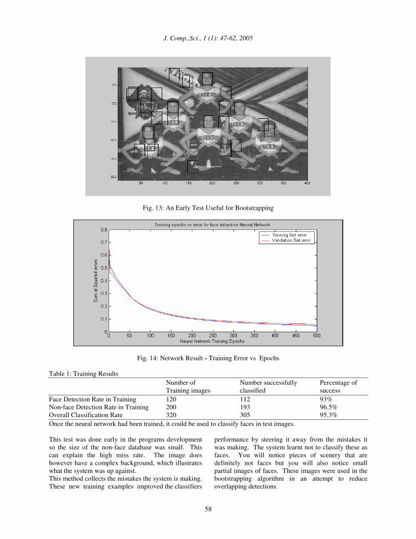
perform. An ideal scenario would be to give the network as large a set of training examples as possible, in order to attain a comprehensive sampling of a larger representation of faces. Images from the Yale face database needed to be resized and cut into 18x27 pixel sizes. 60 face images for entry at the data preparation stage were used to create 120 face training images by taking the left and right compliments of the original image. Each of these images has to be masked with an 18x27 pixel mask and normalised to give a clear face image. Fig. 12 shows a representation of the data at each preparation level. A linear function is applied to each individual image and then subtracted out. This corrects some of the harsh lighting conditions and gives a clear representation of the image. The mask applied to each image clearly defines the face shape. The network looks for faces that fit this aspect. You can see the resultant images have approximately the same grey level distribution. The scanning part of the program employs these steps to each window that is scanned from every test image. A function that attempts to equalise the intensity values across the window is run. Pixels outside the oval mask are ignored so the values in this area are not considered when approximating the lighting correction. The linear function approximates the overall brightness of each part of the image being considered. The result is then subtracted from the window to compensate for the variety of lighting conditions. This normalisation technique is very important for the functioning of the network. An early approach was to use random non-face images to train the early network. These were input intending the network to classify them as negative examples and to give an output of -0.9 (not face). We discovered that these do not benefit the learning process at all. The randomness of the structure of the images we created did nothing to boost the accuracy of the network when early testes were run. The next step was to add a number of all black images to the training set. This approach proved more beneficial, and clearly provided a benefit to the network’s ability to classify. The flat black image provided a baseline for the network to compare to when classifying. We then proceeded to find a more realistic set of training non-face images. Early tests were performed on image which contained no faces just a typical background. If the program detected any positive results from this image they had to be non-faces. These detects are non-face examples with high information value that resemble the face vectors in the neural network. These ‘valid’ non-faces are more useful when presented as non-face training images. The non-face database can grow very large so this method guarantees that the non-face values are not redundant information for the network. Fig. 13 shows an early test on an image with faces detected but there is also a high rate of detections of non-face images.

J. Comp.,Sci., 1 (1): 47-62, 2005

58

Fig. 13: An Early Test Useful for Bootstrapping

Fig. 14: Network Result - Training Error vs Epochs Table 1: Training Results Number of Number successfully Percentage of Training images classified success Face Detection Rate in Training 120 112 93% Non-face Detection Rate in Training 200 193 96.5% Overall Classification Rate 320 305 95.3% Once the neural network had been trained, it could be used to classify faces in test images. This test was done early in the programs development so the size of the non-face database was small. This can explain the high miss rate. The image does however have a complex background, which illustrates what the system was up against. This method collects the mistakes the system is making. These new training examples improved the classifiers

performance by steering it away from the mistakes it was making. The system learnt not to classify these as faces. You will notice pieces of scenery that are definitely not faces but you will also notice small partial images of faces. These images were used in the bootstrapping algorithm in an attempt to reduce overlapping detections.

J. Comp.,Sci., 1 (1): 47-62, 2005

59

Implementation of Training Algorithm: The classifiers task is to identify face test patterns from non-face test patterns based on vectors produced by training images. This training stage defines the network to carry out this task. At this stage we presume that our data set, both face and non-face has been prepared and is ready for input to the network. The training program loads all the required training data and starts to train the network. We used a multi-layer perceptron network to perform the classification task. Each of the 400 input variables of each training image was entered in vector form. The network has 1 output unit and 25 hidden units. Each hidden and output unit computes a weighted sum of its input links and performs Tan sigmoidal thresholding on its output. The output unit returns a 0.9 if a face is detected and -0.9 if otherwise. The Network is trained with the back-propagation learning algorithm until the output error stabilises (or until training reaches 500 epochs). Fig. 14 shows the training result. The sum of squared error rate on the training set over 500 epochs for the Validation set error (red) and Training Set error (blue). Note that around epoch 50 the validation set error surpasses the training set error. However the validation set error never increases from a previous time step and therefore the network proceeds to an approximate convergence. This suggests that the training set is good enough to detect a face image that is not contained in the training set by approximating the faces values to suit a positive detection. After the training of the network we can determine from the network parameters how well the training images were classified. The current performance of the network is shown in Table 1. Note that this is the most recent performance of the network with the final training set after extensive bootstrapping. The network performs much better at detecting non-faces. This is due to the amount of images made available in the dataset it is therefore more bias towards detecting non-faces. This leads to a lower false positive rate than if

the bias had been in the favour of face images instead. Realisation of Scanning and Detecting a Face: Since the scanning window is fixed at 18x27 pixels a means of scaling the image had to be implemented in order to detect faces of multiple sizes in multiple sized images. This is implemented by scaling an image’s resolution by a factor of 1.2. The image is scaled several times to realise detection of an 18x27 window at different image sizes. Fig. 15 shows an image of 200x130 in pixel size. When it was passed through the scanning routine, its image pyramid for six levels is shown in Fig. 16.

Fig. 15: Original Image In Fig. 16, Level 1 is the original image with the same parameters and picture quality but level 2 has parameters of 108 x 166 pixels. This is a result of the scale factor of 1.2. This scaling continues to level six where the resolution is approx 80x50. Keep in mind that the scanning routine will scan every 18x27 window at every level. The classifier should not pick up an 18x27 face in level 1 as the face present is too large. The program should not classify any positive detects until the level has reached a certain point where the face’s resolution lies in a 18x27 bounding box. In fact the test image was run through the program and returned one positive value at level 6. This result is shown below in Fig. 17.

Fig. 16: Resolution Pyramid

J. Comp.,Sci., 1 (1): 47-62, 2005

60

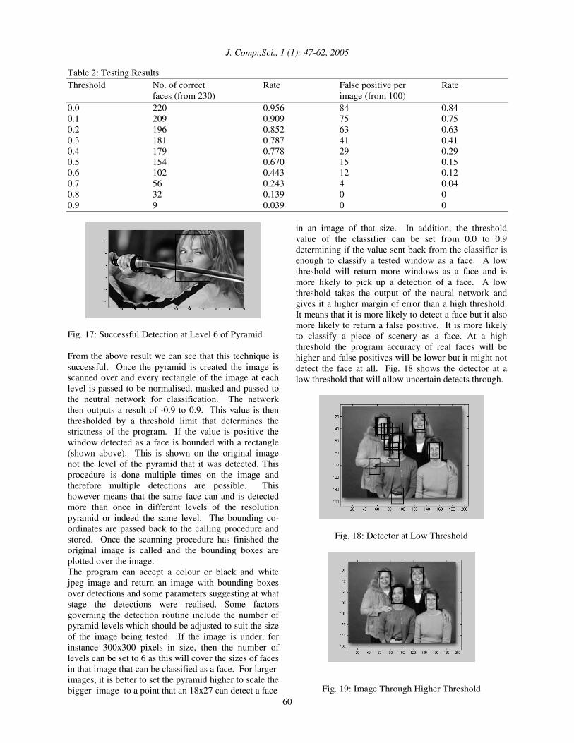
Table 2: Testing Results Threshold No. of correct Rate False positive per Rate faces (from 230) image (from 100) 0.0 220 0.956 84 0.84 0.1 209 0.909 75 0.75 0.2 196 0.852 63 0.63 0.3 181 0.787 41 0.41 0.4 179 0.778 29 0.29 0.5 154 0.670 15 0.15 0.6 102 0.443 12 0.12 0.7 56 0.243 4 0.04 0.8 32 0.139 0 0 0.9 9 0.039 0 0

Fig. 17: Successful Detection at Level 6 of Pyramid From the above result we can see that this technique is successful. Once the pyramid is created the image is scanned over and every rectangle of the image at each level is passed to be normalised, masked and passed to the neutral network for classification. The network then outputs a result of -0.9 to 0.9. This value is then thresholded by a threshold limit that determines the strictness of the program. If the value is positive the window detected as a face is bounded with a rectangle (shown above). This is shown on the original image not the level of the pyramid that it was detected. This procedure is done multiple times on the image and therefore multiple detections are possible. This however means that the same face can and is detected more than once in different levels of the resolution pyramid or indeed the same level. The bounding co-ordinates are passed back to the calling procedure and stored. Once the scanning procedure has finished the original image is called and the bounding boxes are plotted over the image. The program can accept a colour or black and white jpeg image and return an image with bounding boxes over detections and some parameters suggesting at what stage the detections were realised. Some factors governing the detection routine include the number of pyramid levels which should be adjusted to suit the size of the image being tested. If the image is under, for instance 300x300 pixels in size, then the number of levels can be set to 6 as this will cover the sizes of faces in that image that can be classified as a face. For larger images, it is better to set the pyramid higher to scale the bigger image to a point that an 18x27 can detect a face

in an image of that size. In addition, the threshold value of the classifier can be set from 0.0 to 0.9 determining if the value sent back from the classifier is enough to classify a tested window as a face. A low threshold will return more windows as a face and is more likely to pick up a detection of a face. A low threshold takes the output of the neural network and gives it a higher margin of error than a high threshold. It means that it is more likely to detect a face but it also more likely to return a false positive. It is more likely to classify a piece of scenery as a face. At a high threshold the program accuracy of real faces will be higher and false positives will be lower but it might not detect the face at all. Fig. 18 shows the detector at a low threshold that will allow uncertain detects through.

Fig. 18: Detector at Low Threshold

Fig. 19: Image Through Higher Threshold

J. Comp.,Sci., 1 (1): 47-62, 2005

61

You can see from the image that the faces that exist in the image are clearly defined and located by the detector but the amount of false positives in the image outweighs the amount of correct detects. Fig. 19 shows the same image entered into the same network but the threshold at which detects are accepted has been increased. The image show that there is no false detects but there is overlapping of bounding boxes. This means the same face occupied a region that was scanned twice and both times the information of face data passed to the neural network was enough to warrant a successful detection.

RESULTS Fig. 20 through to Fig. 25 show a range of example test results. Fig. 20 is an image ideally suited to the face detection system as it has a simple background with nothing in it to confuse as a face and the face is facing forward (like most of the training set). Fig. 21 however shows a face candidate amongst a complex background. It has the likelihood to return some false positives. Use of the training set however, resulted in restricting it to a small number of false positives.

Fig. 20: Simple Background Image

Fig. 21: Complex Background Image Figure 22 shows an image with more than one face – It needed to return multiple detects. Note the background of the image is not interfering with the image and will not give false positives. Figure 23 shows an image with a face which is undetected due to it position. If it had have been frontal it may have been detected.

Fig. 22: Image with Multiple Detects

Fig. 23: No Detect Figure 24 is a large image with dimensions of 300x400 pixels. The total number of scale levels was set to 8 and the face was detected with ease.

Fig. 24: Successful Detection 2

Fig. 25: Detection at Different Levels

J. Comp.,Sci., 1 (1): 47-62, 2005

62

Figure 25 shows detection at different levels of the pyramid. It has detected them at different scales and positions demonstrating that the network can generalise well. The successfulness of the system depends on how well the network was trained. The speed and accuracy of the system is dependant on a set of parameters that can be adjusted for different results. All training and detection routines where carried out on a PC with a 1.6 GHz Pentium 4 processor with 512 Mb of RAM. The threshold factor denotes how strict the network was when it came to classify the image. Error! Reference source not found. shows the extent of the testing with 100 images (230 faces) ranging from images containing a single face with simple backgrounds (Fig. 20) to complex background (Fig. 21) images with multiple faces (Fig. 22). Each Image had at least one face and there were between 150x150 and 400x400 pixels in size. A total pyramid level of 6, a start pyramid level of 1 and a scale factor of 1.2 were used for all images. In order to achieve high detection rates in a range of images - it also stands to detect more false positives. A very low threshold will detect the same amount of false detections as correct detections. At a high threshold the program gives less false positives but it will also probably fail to detect faces that were just below the threshold. Achieving better face detection rates comes at the cost of increased false positive rates. 220 of the 230 images were detected at 0.0 the lowest threshold. The resultant image from these detections contained a high rate of false detections. A high volume of overlapping bounding boxes showed a random and undefined set of detections. As the testing progressed up through the earlier thresholds (0.1-0.4) a definite pattern was suggested. For each step in the test the number of false positives greatly decreased but some detections were sacrificed. The faces that were sacrificed the most were usually smaller less defined face in group pictures. However, there were also false positives prominent in the higher threshold test areas.

CONCLUSION The Algorithm can detect between 67% and 85% of faces from images of varying size, background and quality with an acceptable number of false detections. It can detect between ‘face’ and ‘non-face’. The normalisation routine which makes training data uniform (especially where lighting is involved) - can drastically affect the classifying of images. The neural network approach is known to be highly sensitive to the grey levels in an image but by subjecting each trained and tested image to the routine the system sidestepped the problem. The bootstrapping algorithm would have beneficiated more if we had continued to update its database. At a very high threshold, only nine faces were detected and five of these were faces from the Yale face database and therefore a part of the training set. Thus with a larger dataset of faces, the program can become more accurate. A threshold of between 0.5-0.6 gives the best range of results out of the threshold set tested. They give a more obvious set of results and continue to detect large faces that produce good data vectors. Detects that are found within this threshold reflect data that is in the training set. This after all was the goal of the system.

REFERENCES 1. Md. Al-Amin Bhuiyan, Shin-yo Muto and

Haruki Ueno, ------. Face Detection and Facial Feature Localisation for Human-machine Interface. National Institute of Informatics

2. Erik Hjelmas and Boon Kee Low, 2001. Face Detection: A Survey Department of Informatics, University of Oslo, Norway.

3. Harley, R.Miller and Arthur R.Weeks, -----. The Pocket Handbook of Image processing Algorithms. ISBN 0-13-6422403

4. Craw, H. Ellis and J. R. Lishman, 1987. Automatic extraction of face-feature. Pattern Recog. Lett.

5. Yale face database, http://cvc.yale.edu/projects/yalefaces/yalefaces.html

6. Sakai, T., M. Nagao and T. Kanade, 1972. Computer analysis and classification of photographs of human faces.

7. Kah-kay Sung and Tomaso Poggio, 1994. Example –based Learning for View-based Human face Detection.

8. Sirovich, L. and M. Kirby, 1987. Low-dimensional procedure for the characterization of human faces, 519-524.

9. Hjelmas, E. and J. Wroldsen, 1999. Recognizing faces from the eyes only, in Proceedings of the 11th Scandinavian Conference on Image Analysis.

10. Lanitis, C., J. Taylor and T. F. Cootes, 1994. Automatic tracking, coding and reconstruction of human faces, using flexible appearance models. IEEE Electron. Lett.

11. Kass, M., A. Witkin and D. Terzopoulos, 1987. Snakes: active contour models. In Proc. of 1st Int Conf. on Computer Vision, London.

12. Cootes, T. F. and C. J. Taylor, 1992. Active shape models—‘smart snakes’. In Proc. of British Machine Vision Conference,pp: 266-275.

13. Sirovich, L. and M. Kirby, 1987. Low-dimensional procedure for the characterization of human faces. J. Opt. Soc. Amer. 4: 519-524.

14. Asim Shankar and Priyendra Singh Deshwal, 2002. Face Detection in images : Neural networks & Support Vector Machines.

15. Martin, H. Hunke, 1994. Locating and Tracking of Human Faces with Neural Networks.

16. Rowley, H. A., S. Baluja and T. Kanade, 1998. Neural network-based face detection. IEEE Trans. Pattern.

17. De Silva, L. C., K. Aizawa and M. Hatori, 1995. Detection and tracking of facial features by using a facial feature model and deformable circular template. IEICE Trans. Inform. Systems E78–D: 1195–1207.

18. Roth, D., M.H. Yang and N. Ahuja, 2000. A SNOW-based face detector, in Advances in Neural Information Processing Systems 12 (NIPS 12), MIT Press, Cambridge, MA.

19. Osuna, E., R. Freund, F. Girosi, 1997. Training support vector machines: An application to face detection, in IEEE Proc. of Int. Conf. on Computer Vision & Pattern Recognition.

20. Vapnik, V., 1995. The Nature of Statistical Learning Theory. Springer-Verlag, NY.

21. Jiang, X., M. Binkert, B. Achermann and H. Bunke, 2000. Towards detection of glasses in facial images. Pattern Anal. Appl.