Embed Size (px)
Citation preview

University of Southern Queensland
Faculty of Engineering and Surveying
The use of low-cost photogrammetry techniques to create an
accurate model of a human skull.
A dissertation submitted by:
Heidi Jane Belbin
W0109098
In fulfilment of the requirements of:
Bachelor of Spatial Science (Honours)
(Major: Surveying)
2015

i
Abstract
There has been increasing interest in low-cost close range photogrammetry techniques for use in a
variety of applications. The use of these techniques in medicine, forensic science, architecture,
engineering, archaeology and anthropology to record, measure and monitor objects and sites has been
growing in recent years. Close range photogrammetry has been particularly investigated and preferred
for human body mapping due to being non-contact, non-invasive, accurate, and inexpensive and data
is re-measurable.
Skulls have been traditionally measured using callipers and tape in anthropological study, which is
subject to observer error. Close range photogrammetry can be used to perform more accurate
measurements and retain a digital copy of the skull, which can be re-used for a number of purposes.
Using low cost software (Photomodeler), and low cost cameras, the aim of this project is to detail the
camera calibration techniques and image capture of a skull. The process for 3D modelling using close
range photogrammetry includes camera calibration to determine the camera’s internal parameters,
photographing the object within a control target frame, and processing the data with photogrammetry
software.
Achieving a high precision camera calibration and producing a high-accuracy 3D model were more
difficult than anticipated. There are a number of factors which can result in a poor quality models.
However, the results show that photogrammetry can be utilised in the capture of accurate 3D skull
model using low-cost cameras efficiently. The research was successful, the project objectives were
satisfied and the accuracy across the project was approximately 0.4mm.
ii
Disclaimer
University of Southern Queensland
Faculty of Health, Engineering and Sciences
ENG4111/ENG4112 Research Project
Limitations of Use
The Council of the University of Southern Queensland, its Faculty of Health, Engineering & Sciences,
and the staff of the University of Southern Queensland, do not accept any responsibility for the truth,
accuracy or completeness of material contained within or associated with this dissertation.
Persons using all or any part of this material do so at their own risk, and not at the risk of the Council
of the University of Southern Queensland, its Faculty of Health, Engineering & Sciences or the staff
of the University of Southern Queensland.
This dissertation reports an educational exercise and has no purpose or validity beyond this exercise.
The sole purpose of the course pair entitled “Research Project” is to contribute to the overall education
within the student’s chosen degree program. This document, the associated hardware, software,
drawings, and other material set out in the associated appendices should not be used for any other
purpose: if they are so used, it is entirely at the risk of the user.

iii
Candidates Certification
I certify that the ideas, designs and experimental work, results, analysis and conclusions set out in this
dissertation are entirely my own efforts, except where otherwise indicated and acknowledged.
I further certify that the work is original and has not been previously submitted for assessment in any
other course or institution, except where specifically stated.
Heidi Jane Belbin
Student Number: W0109098
(Signature)
28/10/2015
(Date)

iv
Acknowledgments
This project was carried out under the principal supervision of Dr. Albert Kon-Fook Chong, in which
I express my sincere and greatest appreciation for his time and guidance in this project. I would also
like to acknowledge Dr Glenn Campbell for his initial guidance in choosing a project.
I would like to express my appreciation to the Surveying and Spatial Sciences Institute (SSSI) for
awarding me the Women in Spatial Scholarship 2015.
I am grateful to all who have helped and given me support during this project.
v
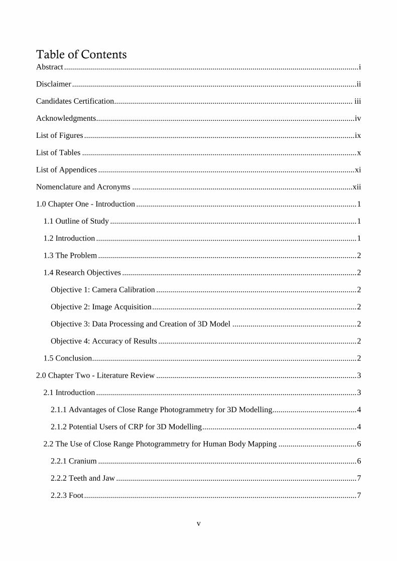
Table of Contents Abstract ................................................................................................................................................... i
Disclaimer .............................................................................................................................................. ii
Candidates Certification....................................................................................................................... iii
Acknowledgments................................................................................................................................. iv
List of Figures ....................................................................................................................................... ix
List of Tables ......................................................................................................................................... x
List of Appendices ................................................................................................................................ xi
Nomenclature and Acronyms .............................................................................................................. xii
1.0 Chapter One - Introduction .............................................................................................................. 1
1.1 Outline of Study ........................................................................................................................... 1
1.2 Introduction .................................................................................................................................. 1
1.3 The Problem ................................................................................................................................. 2
1.4 Research Objectives ..................................................................................................................... 2
Objective 1: Camera Calibration .................................................................................................... 2
Objective 2: Image Acquisition ...................................................................................................... 2
Objective 3: Data Processing and Creation of 3D Model .............................................................. 2
Objective 4: Accuracy of Results ................................................................................................... 2
1.5 Conclusion .................................................................................................................................... 2
2.0 Chapter Two - Literature Review .................................................................................................... 3
2.1 Introduction .................................................................................................................................. 3
2.1.1 Advantages of Close Range Photogrammetry for 3D Modelling.......................................... 4
2.1.2 Potential Users of CRP for 3D Modelling ............................................................................. 4
2.2 The Use of Close Range Photogrammetry for Human Body Mapping ....................................... 6
2.2.1 Cranium ................................................................................................................................. 6
2.2.2 Teeth and Jaw ........................................................................................................................ 7
2.2.3 Foot ........................................................................................................................................ 7
vi
2.2.4 Hand....................................................................................................................................... 9
2.2.5 Spine ...................................................................................................................................... 9
2.3 Complete Body Mapping ........................................................................................................... 10
2.3.1 Forensic Applications .......................................................................................................... 10
2.4 Movement Mapping ................................................................................................................... 11
2.5 Camera Calibration .................................................................................................................... 12
2.5.1 Camera Parameters .............................................................................................................. 12
2.5.2 Calibration Methods ............................................................................................................ 14
2.6 Photomodeler ............................................................................................................................. 15
2.6.1 Accuracy of Photomodeler .................................................................................................. 16
2.6.2 Applications for Photomodeler Software ............................................................................ 17
2.6.3 Advantages and Disadvantages of Photomodeler ............................................................... 18
2.7 Summary .................................................................................................................................... 18
3.0 Chapter Three – Research Design and Methodology .................................................................... 20
3.1 Objectives ................................................................................................................................... 20
1. Camera Calibration ................................................................................................................... 20
2. Image Acquisition..................................................................................................................... 20
3. Data Processing and Creation of 3D Model ............................................................................. 20
4. Accuracy ................................................................................................................................... 20
3.2 Implications of Research ............................................................................................................ 20
3.3 Equipment .................................................................................................................................. 20
3.3.1 Cameras ............................................................................................................................... 20
3.3.2 Photogrammetry Software ................................................................................................... 20
3.3.3 Targets ................................................................................................................................. 21
3.3.4 Skull ..................................................................................................................................... 21
3.3.5 Callipers and Tape ............................................................................................................... 21
3.3.6 Miscellaneous ...................................................................................................................... 21

vii
3.4 Camera Calibration .................................................................................................................... 21
3.4.1 Target Type and Size ........................................................................................................... 21
3.4.2 Calibration Method .............................................................................................................. 22
3.4.3 Camera and Calibration Grid Position ................................................................................. 22
3.5 Target Configuration .................................................................................................................. 23
3.6 Image Acquisition ...................................................................................................................... 24
3.6.1 Texture of the Object ........................................................................................................... 24
3.6.2 Lighting ............................................................................................................................... 25
3.6.3 Background .......................................................................................................................... 25
3.6.4 Camera Position and Angles ................................................................................................ 25
3.6.5 Camera Settings ................................................................................................................... 26
3.7 Processing................................................................................................................................... 26
3.7.1 Uploading Photos ................................................................................................................ 26
3.7.2 Automatic Target Marking .................................................................................................. 26
3.7.3 Processing ............................................................................................................................ 27
3.7.4 DSM Trim............................................................................................................................ 28
3.7.5 Create DSM ......................................................................................................................... 28
3.8 Creation of the 3D Model........................................................................................................... 29
3.9 Assessment of Accuracy ............................................................................................................ 31
4.0 Chapter Four – Results and Discussion ......................................................................................... 33
4.1 Camera Calibration .................................................................................................................... 33
4.1.1 Results of Calibration .......................................................................................................... 34
4.1.2 Discussion of Calibration Results........................................................................................ 35
4.2 Photograph Capture and Processing ........................................................................................... 36
4.2.1 Discussion of Model Results ............................................................................................... 37
4.3 Measurements and Accuracy ..................................................................................................... 38
4.3.1 Skull Measurements ............................................................................................................ 38

viii
4.3.2 Check on Accuracy .............................................................................................................. 39
4.3.3 Discussion of Results ........................................................................................................... 39
4.3.4 Summary of Objectives Achieved ....................................................................................... 39
5.0 Chapter Five - Conclusions ............................................................................................................ 41
5.1 Introduction ................................................................................................................................ 41
5.2 Conclusions ................................................................................................................................ 41
5.3 Further Research and Recommendations ................................................................................... 42
References ............................................................................................................................................ 43
Appendix A: Project Specification ...................................................................................................... 47
Appendix B: Photomodeler Referenced Material ................................................................................ 48
Appendix C: Processing Report ........................................................................................................... 49
Appendix D: Creating a 3D Dense Surface ......................................................................................... 53

ix
List of Figures
Page
Figure 2.1 The principle of photogrammetric measurement. 3
Figure 2.2 The effect of radial distortion on the lens. 13
Figure 2.3 Vertical misalignment of the camera lens. 13
Figure 2.4 Range of Photomodeler software. 16
Figure 3.1 Configuration of target camera positions and orientations. 22
Figure 3.2 Create Coded Targets window in Photomodeler. 24
Figure 3.3 Skull showing location of camera stations. 25
Figure 3.4 Automatic Target Marking options window in Photomodeler. 26
Figure 3.5 Processing options window in Photomodeler. 27
Figure 3.6 Photo configuration and Create Dense Surface options in Photomodeler. 29
Figure 3.7 Export options in Photomodeler and resulting DXF file in AutoCAD. 30
Figure 3.8 Screen shot of Photomodeler showing the Measurements pane. 31
Figure 3.9 Screen shot showing measurements between selected targets. 32
Figure 4.1 Overall RMS for all three sets. 33
Figure 4.2 Maximum residuals for all three sets. 33
Figure 4.3 DSM coloured with photo texture and single texture with points coloured
with photo texture. 36
Figure 4.4 DSM with points coloured by depth, photo texture overlaid with point cloud,
triangulated mesh and DSM showing close correlation with point cloud
underneath.
36
Figure 4.5 DSM with comments. 37
Figure 4.6 Skull showing measurements mentioned in Tables 4.3 and 4.4 38

x
List of Tables
Page
Table 2.1 A sample of papers which used PM in their research and stated the accuracy
achieved. 17
Table 3.1 Indicators of quality in the processing report. 28
Table 4.1 Calibration sets completed and comments. 33
Table 4.2 Camera calibration results showing parameters, Root Mean Squared (RMS) and
Maximum Residual 34
Table 4.3 Measurements taken on skull. 38
Table 4.4 Check measurements between targets. 39

xi
List of Appendices
Page
Appendix A Project Specification 47
Appendix B Photomodeler Referenced Material 48
Appendix C Processing Report (Raw File) 49
Appendix D Creating a 3D Dense Surface 53

xii
Nomenclature and Acronyms
2D Two Dimensional
3D Three Dimensional
CBCT Cone Beam Computed Tomography
CCD Coupled Charged Diode
CMOS Complementary Metal-Oxide Semiconductor
CT Computed Tomography
CRP Close Range Photogrammetry
MRI Magnetic Resonance Imaging
PM Photomodeler
RMS Root Mean Squared
1
1.0 Chapter One - Introduction
1.1 Outline of Study
This project involves testing the suitability and accuracy of low cost close range photogrammetry
(CRP) for modelling a complex object, such as a human skull. Human skulls are important for the
study of anthropology, archaeology, medicine, forensic identification to name a few applications. CRP
is preferable to other methods of capturing data as it is low cost, accurate, non-invasive, non-contact,
time efficient, photos and model are re-measurable, inaccessible spots can be photographed and able
to be performed by professionals outside of the photogrammetry or spatial science field.
The project will assess the ease and simplicity of using Photomodeler to create a 3D model of a model
human skull, as well as the accuracy attained. The Project Specification can be found in Appendix A.
1.2 Introduction
Low cost CRP is increasing in popularity as a method of capturing data to create accurate, true to scale
3D models of objects and scenes. There are a number of advantages of using CRP compared with other
data capture methods, such as laser scanning. The advantages include:
High accuracy
Low cost
Ease of use
Portability
Non-contact and non-invasive
The validity of the claims above as made by various research papers will be tested, by attempting to
create a 3D model of a human skull using low cost CRP techniques, equipment and software, in which
the following criteria will be assessed:
Accuracy of camera calibration
Quality of software processing (image to model quality)
Ease of use
Accuracy of the model
Any problems or difficulties encountered
2
1.3 The Problem
Low cost CRP is becoming an increasingly widely used tool for capturing data for a range of
applications. Photogrammetry software, such as Photomodeler, is marketed as being easy to use and
can produce 3D models of high accuracy and quality. A complex object, such as a human skull, is an
appropriate and real-world subject to test the ease at which a 3D model can be created using
Photomodeler, as well as the accuracy which can be achieved by a non-professional (undergraduate
student) using low cost equipment and basic photogrammetry techniques. There are difficulties in
creating complex, 3D objects using CRP and methods for improving data capture are needed.
1.4 Research Objectives
Objective 1: Camera Calibration
Determine the most appropriate calibration for the task, including the coded target type, number of
targets and discuss any differences between the two cameras.
Objective 2: Image Acquisition
Determine the optimal amount of targets to be used and configuration.
Objective 3: Data Processing and Creation of 3D Model
Analyse the level of difficulty and note any problems in the creation of the 3D model from the images.
Objective 4: Accuracy of Results
Assess the accuracy of the 3D model comparing measurements taken with callipers and tape.
1.5 Conclusion
This project aims to be a practical demonstration and a test of the accuracy that can be achieved using
CRP techniques and a low cost, off the shelf camera in modelling a complex object, such as a human
skull. During the case study, any difficulties during calibration, image acquisition and processing are
to be noted and discussed. The literature review discusses advantages and problems researchers have
experienced using low cost CRP and software for their particular applications. The case study in this
project should help to uncover potential difficulties and good practice that may help to guide others in
their use of low cost CRP.
3
2.0 Chapter Two - Literature Review
2.1 Introduction
The use of low cost CRP to create 3D models is a somewhat new tool, which has its roots in a longer
history (Fryer, Mitchell & Chandler 2007, p. 1), that researchers in different professions are
investigating the applications where CRP can be useful. CRP is becoming increasingly popular as a
tool for data capture in fields outside of spatial science. For this reason it is important to investigate
thoroughly how CRP has been used in a variety of applications and the appropriateness of the tool for
the task. It is the role of spatial scientists to investigate technology and advise the professional
community in the appropriate use and limitations of data.
The principles of photogrammetry involve the fundamental sciences of mathematics, physics,
information sciences and biology. (Luhmann et al. 2006, p. 3) CRP has varied applications and a strong
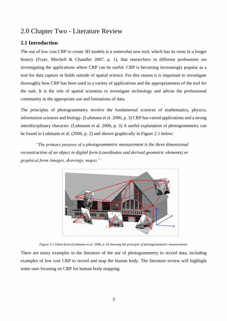
interdisciplinary character. (Luhmann et al. 2006, p. 3) A useful explanation of photogrammetry can
be found in Luhmann et al. (2006, p. 2) and shown graphically in Figure 2.1 below:
“The primary purpose of a photogrammetric measurement is the three dimensional
reconstruction of an object in digital form (coordinates and derived geometric elements) or
graphical form (images, drawings, maps).”
Figure 2.1 Taken from (Luhmann et al. 2006, p. 6) showing the principle of photogrammetric measurement.
There are many examples in the literature of the use of photogrammetry to record data, including
examples of low cost CRP to record and map the human body. The literature review will highlight
some uses focusing on CRP for human body mapping.
4
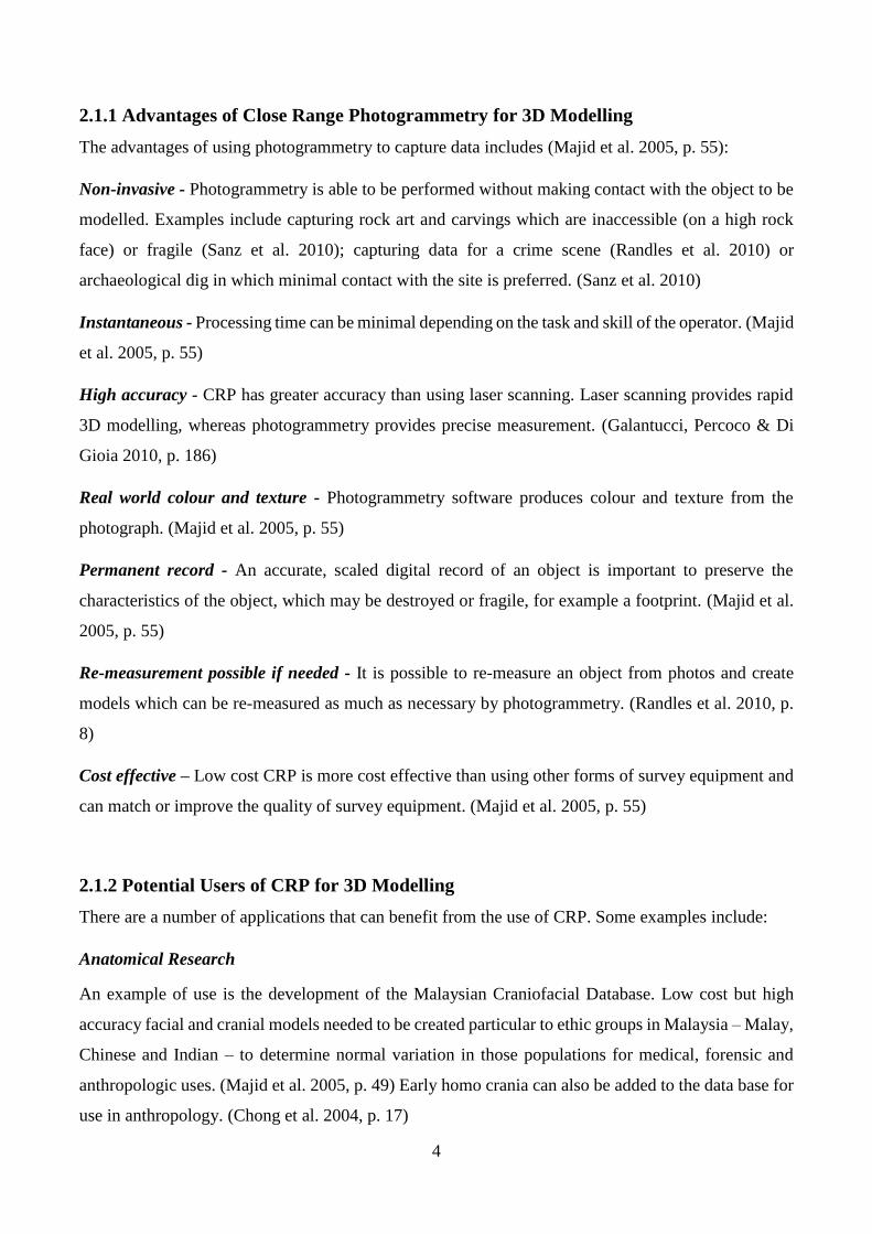
2.1.1 Advantages of Close Range Photogrammetry for 3D Modelling
The advantages of using photogrammetry to capture data includes (Majid et al. 2005, p. 55):
Non-invasive - Photogrammetry is able to be performed without making contact with the object to be
modelled. Examples include capturing rock art and carvings which are inaccessible (on a high rock
face) or fragile (Sanz et al. 2010); capturing data for a crime scene (Randles et al. 2010) or
archaeological dig in which minimal contact with the site is preferred. (Sanz et al. 2010)
Instantaneous - Processing time can be minimal depending on the task and skill of the operator. (Majid
et al. 2005, p. 55)
High accuracy - CRP has greater accuracy than using laser scanning. Laser scanning provides rapid
3D modelling, whereas photogrammetry provides precise measurement. (Galantucci, Percoco & Di
Gioia 2010, p. 186)
Real world colour and texture - Photogrammetry software produces colour and texture from the
photograph. (Majid et al. 2005, p. 55)
Permanent record - An accurate, scaled digital record of an object is important to preserve the
characteristics of the object, which may be destroyed or fragile, for example a footprint. (Majid et al.
2005, p. 55)
Re-measurement possible if needed - It is possible to re-measure an object from photos and create
models which can be re-measured as much as necessary by photogrammetry. (Randles et al. 2010, p.
8)
Cost effective – Low cost CRP is more cost effective than using other forms of survey equipment and
can match or improve the quality of survey equipment. (Majid et al. 2005, p. 55)
2.1.2 Potential Users of CRP for 3D Modelling
There are a number of applications that can benefit from the use of CRP. Some examples include:
Anatomical Research
An example of use is the development of the Malaysian Craniofacial Database. Low cost but high
accuracy facial and cranial models needed to be created particular to ethic groups in Malaysia – Malay,
Chinese and Indian – to determine normal variation in those populations for medical, forensic and
anthropologic uses. (Majid et al. 2005, p. 49) Early homo crania can also be added to the data base for
use in anthropology. (Chong et al. 2004, p. 17)

5
Surgery, Medicine and Dentistry
There is a wide variety of medical applications for CRP, including monitoring for disease, post and
pre surgery assessment, and studies of motion. Photogrammetry has been used in dentistry to allow
accurate models of teeth to be created to study bite contact in the jaw and teeth. (Shigeta et al. 2013)
Detailed examples of the use of low cost CRP in the medical field are discussed later.
Forensic Science
Vehicle accident reconstruction is another application (Randles et al. 2010) and also crime scene
investigation. (Chong et al. 2004, p.17) Photogrammetry allows a record of a crash or crime scene to
be kept and re-examined at any time. (Randles et al. 2010, p. 8) Randles et al (2010, p.8) make the
comment that photogrammetry has advantages over using a total station in that potential mistakes can
be more easily seen and fixed; and that points can be missed when measuring using a total station,
which are not noticed until the data is downloaded, making corrections difficult.
Archaeology and Heritage
CRP has gained popularity in archaeological research for applications such as recording, analysis, and
creating accurate models of artefacts and rock faces (Sanz et al. 2010) and recording burial sites.
(Dellepiane et al. 2013) ‘Analogue’ recording of artefacts is limited in the knowledge that can be
displayed, including the ability to re-examine if the artefact should be destroyed or lost. (Krajňák,
Pukanská & Bartoš 2011, p. 337)
It has also become a concern to give the general public access to archaeological and historical objects
and sites in 3D, especially in this age of web technology and virtual reality. (Guarnieri, Pirotti &
Vettore 2010) and (Krajňák, Pukanská & Bartoš 2011) Photogrammetry could help to provide data for
those applications.
Architecture
CRP has become a tool for monitoring and recording heritage buildings and has applications within
architecture as well. (De Reu et al. 2013) Hernán-Pérez et al. (2013) have examined the usage of a
smart phone camera and CRP for architecture students to help learning within their field.
Engineering
Generally, the uses of CRP in engineering have involved the analysis of manufactured components,
measurement of large structures and objects, to measure in difficult environments or perform on going
measurements and testing of moving objects. (Fryer, Mitchell & Chandler 2007, p. 67)
6
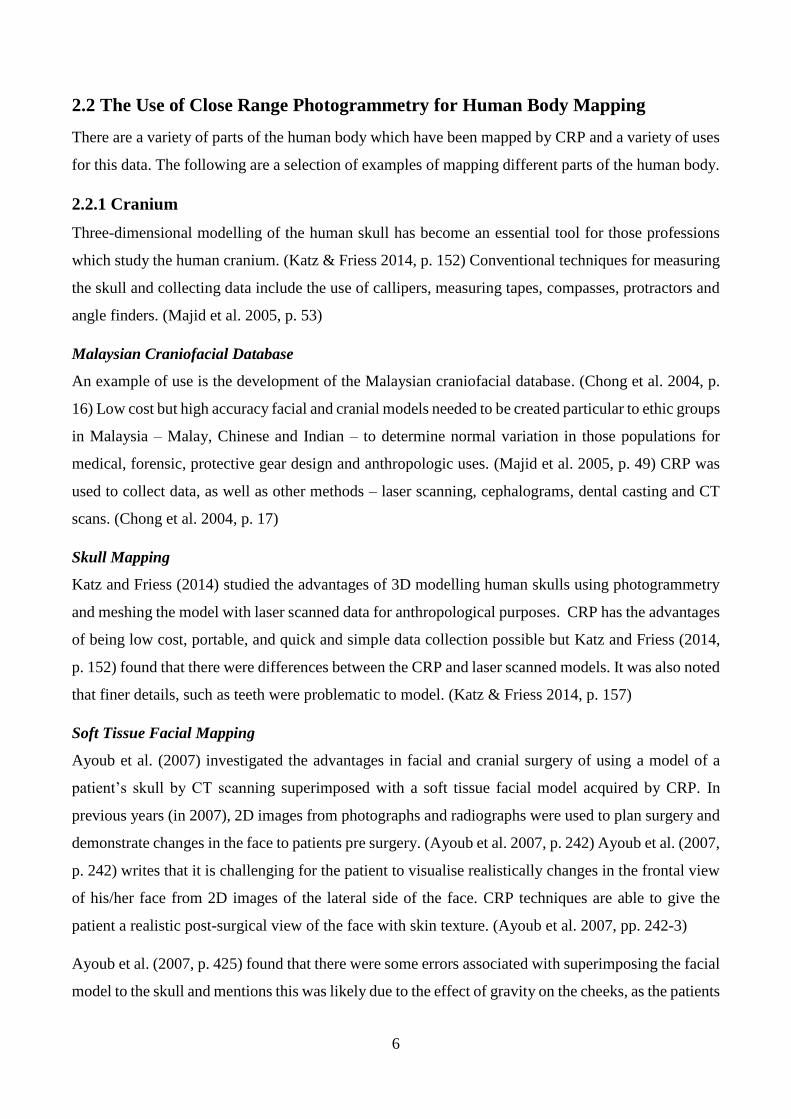
2.2 The Use of Close Range Photogrammetry for Human Body Mapping
There are a variety of parts of the human body which have been mapped by CRP and a variety of uses
for this data. The following are a selection of examples of mapping different parts of the human body.
2.2.1 Cranium
Three-dimensional modelling of the human skull has become an essential tool for those professions
which study the human cranium. (Katz & Friess 2014, p. 152) Conventional techniques for measuring
the skull and collecting data include the use of callipers, measuring tapes, compasses, protractors and
angle finders. (Majid et al. 2005, p. 53)
Malaysian Craniofacial Database
An example of use is the development of the Malaysian craniofacial database. (Chong et al. 2004, p.
16) Low cost but high accuracy facial and cranial models needed to be created particular to ethic groups
in Malaysia – Malay, Chinese and Indian – to determine normal variation in those populations for
medical, forensic, protective gear design and anthropologic uses. (Majid et al. 2005, p. 49) CRP was
used to collect data, as well as other methods – laser scanning, cephalograms, dental casting and CT
scans. (Chong et al. 2004, p. 17)
Skull Mapping
Katz and Friess (2014) studied the advantages of 3D modelling human skulls using photogrammetry
and meshing the model with laser scanned data for anthropological purposes. CRP has the advantages
of being low cost, portable, and quick and simple data collection possible but Katz and Friess (2014,
p. 152) found that there were differences between the CRP and laser scanned models. It was also noted
that finer details, such as teeth were problematic to model. (Katz & Friess 2014, p. 157)
Soft Tissue Facial Mapping
Ayoub et al. (2007) investigated the advantages in facial and cranial surgery of using a model of a
patient’s skull by CT scanning superimposed with a soft tissue facial model acquired by CRP. In
previous years (in 2007), 2D images from photographs and radiographs were used to plan surgery and
demonstrate changes in the face to patients pre surgery. (Ayoub et al. 2007, p. 242) Ayoub et al. (2007,
p. 242) writes that it is challenging for the patient to visualise realistically changes in the frontal view
of his/her face from 2D images of the lateral side of the face. CRP techniques are able to give the
patient a realistic post-surgical view of the face with skin texture. (Ayoub et al. 2007, pp. 242-3)
Ayoub et al. (2007, p. 425) found that there were some errors associated with superimposing the facial
model to the skull and mentions this was likely due to the effect of gravity on the cheeks, as the patients

7
were photographed in a supine position, and also the eyebrows and eyelids had errors which may be
associated with facial expressions. Ayoub et al. (2007, p. 243) comments that CRP proved fast and of
acceptable accuracy for their application.
Cevidanes et al. (2010, p. S120) discusses the benefits of using cone beam CT to create 3D facial
models to study soft tissue changes due to growth or treatment and they argue CRP and laser scanning
are not suitable due to a lack of stable references for a changing face over time. Also, head position
and facial expression cause difficulties, and light reflection from the eye lens interferes with the
creation of the 3D model. (Cevidanes et al. 2010, pp. S120-S1) Cevidanes et al. (2010, p. S125) makes
the comment that CT scans have a risk of exposure to radiation and risk of cancer, which CRP does
not.
2.2.2 Teeth and Jaw
Photogrammetry has been used in dentistry to allow accurate models of teeth to be created to study
bite contact in the jaw and teeth. (Shigeta et al. 2013) CRP has been demonstrated to be useful in
monitoring normal and abnormal growth, malformations, surgical planning and evaluation of treatment
in orthodontic surgery. (Galantucci, Percoco & Di Gioia 2010)
2.2.3 Foot
Modelling the foot can provide medical researchers and practitioners with valuable data for a variety
of medical injuries and conditions. Al-Baghdadi et al (2011) examine the use of CRP to map the dorsal
and plantar surfaces of the foot during weight bearing postures, which can be difficult to map. This
information can be used in the design of foot wear and customised orthotics to suit the weigh bearing
dynamics of the foot, which shows more accurately the shape and pressure areas of a foot than models
developed from an immobile, non-weight bearing foot. (Al-Baghdadi et al. 2011, pp. 295-6) Chong
(2011) investigated the suitability of CRP for monitoring the hands and feet of CMT (Charcot-Marie-
Tooth) disease patients for signs of muscle loss and reduced touch sensitivity.
Alshadli, Duaa et al. (2013) investigate CRP measurement of the foot to study links between foot
posture in athletes and repetitive injury. Static and dynamic measurements were taken; static using a
digital calliper and dynamic using CRP techniques. (Alshadli, Duaa et al. 2013, p. 2) It was found there
were differences between the measurements of the static and dynamic postures of areas of the foot
(arch), and comments made that it is important to consider changes in the foot during gait, not only the
static measurements. (Alshadli, Duaa et al. 2013, p. 4)
8
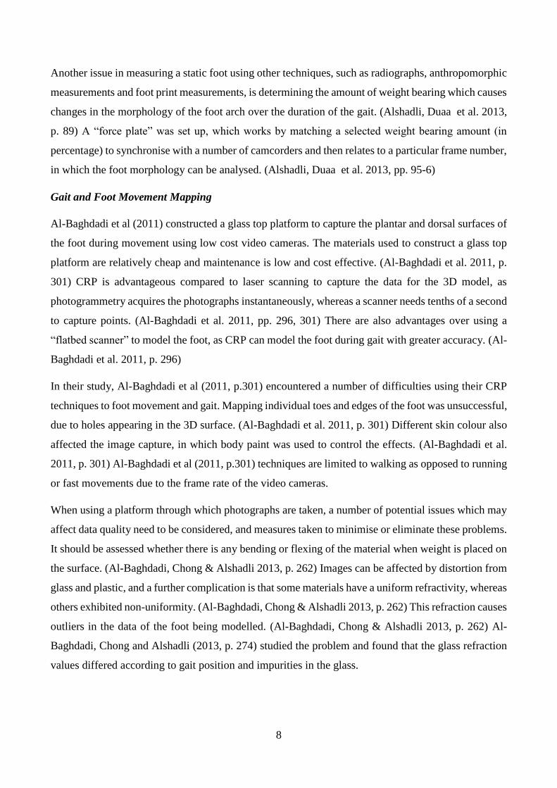
Another issue in measuring a static foot using other techniques, such as radiographs, anthropomorphic
measurements and foot print measurements, is determining the amount of weight bearing which causes
changes in the morphology of the foot arch over the duration of the gait. (Alshadli, Duaa et al. 2013,
p. 89) A “force plate” was set up, which works by matching a selected weight bearing amount (in
percentage) to synchronise with a number of camcorders and then relates to a particular frame number,
in which the foot morphology can be analysed. (Alshadli, Duaa et al. 2013, pp. 95-6)
Gait and Foot Movement Mapping
Al-Baghdadi et al (2011) constructed a glass top platform to capture the plantar and dorsal surfaces of
the foot during movement using low cost video cameras. The materials used to construct a glass top
platform are relatively cheap and maintenance is low and cost effective. (Al-Baghdadi et al. 2011, p.
301) CRP is advantageous compared to laser scanning to capture the data for the 3D model, as
photogrammetry acquires the photographs instantaneously, whereas a scanner needs tenths of a second
to capture points. (Al-Baghdadi et al. 2011, pp. 296, 301) There are also advantages over using a
“flatbed scanner” to model the foot, as CRP can model the foot during gait with greater accuracy. (Al-
Baghdadi et al. 2011, p. 296)
In their study, Al-Baghdadi et al (2011, p.301) encountered a number of difficulties using their CRP
techniques to foot movement and gait. Mapping individual toes and edges of the foot was unsuccessful,
due to holes appearing in the 3D surface. (Al-Baghdadi et al. 2011, p. 301) Different skin colour also
affected the image capture, in which body paint was used to control the effects. (Al-Baghdadi et al.
2011, p. 301) Al-Baghdadi et al (2011, p.301) techniques are limited to walking as opposed to running
or fast movements due to the frame rate of the video cameras.
When using a platform through which photographs are taken, a number of potential issues which may
affect data quality need to be considered, and measures taken to minimise or eliminate these problems.
It should be assessed whether there is any bending or flexing of the material when weight is placed on
the surface. (Al-Baghdadi, Chong & Alshadli 2013, p. 262) Images can be affected by distortion from
glass and plastic, and a further complication is that some materials have a uniform refractivity, whereas
others exhibited non-uniformity. (Al-Baghdadi, Chong & Alshadli 2013, p. 262) This refraction causes
outliers in the data of the foot being modelled. (Al-Baghdadi, Chong & Alshadli 2013, p. 262) Al-
Baghdadi, Chong and Alshadli (2013, p. 274) studied the problem and found that the glass refraction
values differed according to gait position and impurities in the glass.
9
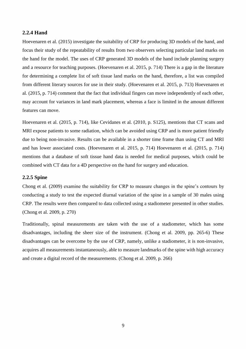
2.2.4 Hand
Hoevenaren et al. (2015) investigate the suitability of CRP for producing 3D models of the hand, and
focus their study of the repeatability of results from two observers selecting particular land marks on
the hand for the model. The uses of CRP generated 3D models of the hand include planning surgery
and a resource for teaching purposes. (Hoevenaren et al. 2015, p. 714) There is a gap in the literature
for determining a complete list of soft tissue land marks on the hand, therefore, a list was compiled
from different literary sources for use in their study. (Hoevenaren et al. 2015, p. 713) Hoevenaren et
al. (2015, p. 714) comment that the fact that individual fingers can move independently of each other,
may account for variances in land mark placement, whereas a face is limited in the amount different
features can move.
Hoevenaren et al. (2015, p. 714), like Cevidanes et al. (2010, p. S125), mentions that CT scans and
MRI expose patients to some radiation, which can be avoided using CRP and is more patient friendly
due to being non-invasive. Results can be available in a shorter time frame than using CT and MRI
and has lower associated costs. (Hoevenaren et al. 2015, p. 714) Hoevenaren et al. (2015, p. 714)
mentions that a database of soft tissue hand data is needed for medical purposes, which could be
combined with CT data for a 4D perspective on the hand for surgery and education.
2.2.5 Spine
Chong et al. (2009) examine the suitability for CRP to measure changes in the spine’s contours by
conducting a study to test the expected diurnal variation of the spine in a sample of 30 males using
CRP. The results were then compared to data collected using a stadiometer presented in other studies.
(Chong et al. 2009, p. 270)
Traditionally, spinal measurements are taken with the use of a stadiometer, which has some
disadvantages, including the sheer size of the instrument. (Chong et al. 2009, pp. 265-6) These
disadvantages can be overcome by the use of CRP, namely, unlike a stadiometer, it is non-invasive,
acquires all measurements instantaneously, able to measure landmarks of the spine with high accuracy
and create a digital record of the measurements. (Chong et al. 2009, p. 266)
10
2.3 Complete Body Mapping
2.3.1 Forensic Applications
Autopsy Records
Urbanová, Hejna and Jurda (2015) investigate the benefits of both CRP and laser scanning to document
autopsies. Three dimensional modelling is useful for the documentation process as re-measurement
and analysis can be made in the future. (Urbanová, Hejna & Jurda 2015, pp. 77-8) This is particularly
relevant to being able to reassess body measurements, wounds, angles of penetration of weapons and
so on. (Urbanová, Hejna & Jurda 2015, p. 78)
In their paper, Urbanová, Hejna and Jurda (2015, pp. 78, 83) commented that CRP in particular was
appealing as it is simple, inexpensive with relatively trivial equipment needs and can be performed
without “special training” or “prior experience.” However, when discussing the results of their case
study, scanning and using CRP to create 3D models of two deceased individuals and one living person,
a number of difficulties were encountered with both techniques. (Urbanová, Hejna & Jurda 2015, p.
84)
In regards to CRP, the model had “scrappy edges” where the bodies touched the autopsy table and in
the living person’s model, there were differences due to body movement, such as breathing.
(Urbanová, Hejna & Jurda 2015, p. 84) There were also some holes in the model due to body hair,
depressions and body fluids, in regards to the images taken when the deceased bodies were opened for
examination. (Urbanová, Hejna & Jurda 2015, p. 85)
Despite these challenges, the CRP derived models showed the entire surface of the body including
areas of greater error, whereas the scanner algorithm will not generate those areas of high error.
(Urbanová, Hejna & Jurda 2015, p. 85) CRP was also able to document in photo-realistic texture the
skin, any blemishes, scars, injuries and tattoos, better than the scanner. (Urbanová, Hejna & Jurda
2015, p. 84) Urbanová, Hejna and Jurda (2015, p. 86) comment that CRP is a useful tool to document
post mortems, but the amount of time needed to process a full body may not be desirable, and that
CRP is better for documenting areas of interest on the body.
Slot, Larsen and Lynnerup (2014) also investigated the benefits of CRP in autopsies, focusing only on
physical measurements of the body, such as measuring the location of wounds. Usually when
performing an autopsy, “areas of interest” on a body, such as wounds, are described in text and
photographed, with measurements of size recorded and location described in relation to a particular
anatomical point. (Slot, Larsen & Lynnerup 2014, p. 226)
11
Further information can sometimes be required after the autopsy, which then is impossible to collect
or re-measure, which is the reason CRP is beneficial to forensic applications, as a 3D model can be
repeatedly re-measured and studied. (Slot, Larsen & Lynnerup 2014, p. 226) Slot, Larsen and
Lynnerup (2014, p. 228) found that the differences between body measurements using a ruler and
using photogrammetry were less than 1cm, which is in an acceptable range for body measurement
purposes.
2.3.2 Height Estimation
A person’s height can be estimated using images and photogrammetry techniques and this is
particularly useful in criminal investigations. Chong (2002) discusses a technique of calibrating
surveillance cameras in situ using a portable target control frame to be able to extract measurements
of suspect’s height, which can be used to identify a person. This technique is not limited to a person
height; it can be used to measure other parts of a body, such as an arm or even a shoe to estimate shoe
size. (Chong 2002, p. 758) Chong (2002, p. 758) writes that the average accuracy of using this
technique was 23mm +/- 7mm.
Hoogeboom, Alberink and Goos (2009, p. 1365) examine the issue of differences between the real
height of a person and the height derived from the images to examine what is the cause of these
differences. In their paper they write that there is a correlation between the camera view side used to
estimate height, the type of camera and the height calculated. (Hoogeboom, Alberink & Goos 2009, p.
1373) Hoogeboom, Alberink and Goos (2009, p. 1375) also comment that the stance of the person
when the height measurements are calculated has an effect on the accuracy of the value.
2.4 Movement Mapping
Low cost video cameras are able to be used to capture human movement using photogrammetric
techniques and software. (Chong 2006, p. 227) There are a wide variety of uses for this kind of data,
including medical applications, such as the foot and gait during walk, discussed previously.
Chong (2006) conducted a study to examine the propulsion of the hand for application in swimming.
CRP was deemed to be useful to this study as photos of the hand during motion can be captured
instantly of both sides of the hand in a multi camera set up, and can be operated underwater. (Chong
2006, p. 74)
12
2.5 Camera Calibration
Calibration is one of the most debated problems in photogrammetry. (Galantucci et al. 2014, p. 279)
Low cost, consumer grade, non-metric cameras are designed for the purpose of photography and need
to be calibrated for photogrammetry usage. (Hassan, Ma'Arof & Samad 2014, p. 123) Calibration
calculates parameters related to the position and rotation of each camera in the 3D space (external
parameters), the focal length and position of the principal point on the sensor (internal parameters),
lens distortion and non-symmetrical components. (Galantucci et al. 2014, p. 280) Another way of
explaining basically what camera calibration aims to achieve, is to quote Hassan, Ma'Arof and Samad
(2014, p. 124), “The purpose of camera calibration is to distinguish wholly the light rays when it was
exposed when entering the camera.”
2.5.1 Camera Parameters
The geometric configuration inside a camera and its lens system is referred to as the interior orientation
of the camera. (Fryer 2001, p. 156) As a lens is never perfect, these imperfections result in a reduction
of image quality and error in the location of the image. (Fryer 2001, p. 157) Radial and decentring
distortion relate to the lens of the camera and affect the location of the image. (Fryer 2001, p. 157)
Format Size
A format size refers to the size (area) of a camera’s imaging chip (CCD or CMOS) which affects the
imaging area of the camera. (EoS Systems Inc. 2015)
Focal Length
Photomodeler provides a simple and useful explanation of focal length, “…the distance between the
imaging plane (e.g. the image chip in a digital camera) and a point where all light rays intersect inside
the lens (the ‘optical centre’).” The principal distance relates to the focal length in that the focal length
is the principal distance when the lens is focus is to infinity. (EoS Systems Inc. 2015)
Principal Distance
The principal point is the distance between the centre of the camera lens and image plane. (Fryer 2001,
p. 158) According to Fryer (2001, p. 158), an approximation of the principal distance and a calculated
value for the coordinates of the image and real world object are satisfactory to obtain the principal
distance for the camera.
Principal Point
The principal point, or the full term, the principal point of autocollimation, refers to the point at which
the true centre of the lens would project in a straight line to the image plane. (Fryer 2001, p. 158) The
13
lens centre is often located imperfectly, thus the focal plane not truly perpendicular to the optical axis,
in which the calibration process will determine the misalignment error and position of the principal
point. (Fryer 2001, p. 158)
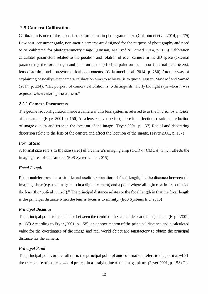
Radial Distortion
Radial distortion can be described as barrel or pin cushion in nature, and can be best demonstrated by
the shape of a rectangle which will appear distorted depending on whether it is located closer or further
from the principal point. (Fryer 2001, p. 159) Figure 2.2 (below) shows the effect radial distortion has
to the lens of the camera.
Figure 2.2 The effect of radial distortion on the lens (Yusoff et al. 2014, p.2)
Radial distortion can be calculated by the formula:
𝛿𝑟 = 𝐾1𝑟3 + 𝐾2𝑟5 + 𝐾3𝑟7 + ⋯
where K1, K2, K3 are coefficients and δr (radial distortion) is in micrometres (μm). (Fryer 2001, pp.
160-1)
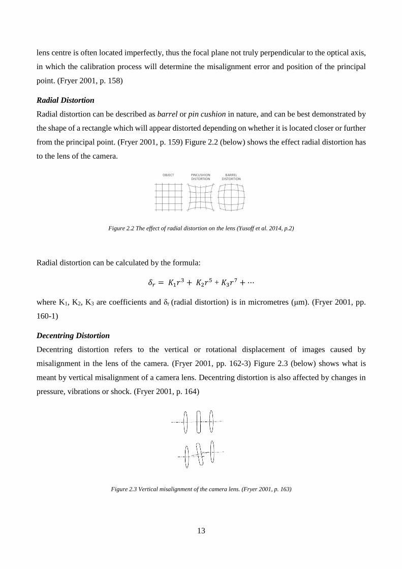
Decentring Distortion
Decentring distortion refers to the vertical or rotational displacement of images caused by
misalignment in the lens of the camera. (Fryer 2001, pp. 162-3) Figure 2.3 (below) shows what is
meant by vertical misalignment of a camera lens. Decentring distortion is also affected by changes in
pressure, vibrations or shock. (Fryer 2001, p. 164)
Figure 2.3 Vertical misalignment of the camera lens. (Fryer 2001, p. 163)
14
2.5.2 Calibration Methods
There are a few methods of camera calibration, which include analytical plumb line, field calibration,
system calibration and self-calibration. Traditionally, calibration was achieved by the use of
coordinated targets measured and calculated using theodolites or images acquired from metric
cameras, in a laboratory setting. (Fryer 2001, p. 165) As CRP has progressed, there is a need for
practical, inexpensive and time efficient calibration methods. (Fryer 2001, p. 165)
Analytical Plumb Line
Analytical plumb line calibration can determine radial and decentring distortion but cannot determine
the principal point or principal distance. (Fryer 2001, p. 168) Its usefulness is often seen as an
independent check for other calibration methods or to ascertain lens distortion trial values for a bundle
adjustment. (Fryer 2001, p. 168) Analytical plumb line calibration involves photographing straight
lines, which may be constructed from fishing line for example, and examining the departure from this
straight line in the image. (Fryer 2001, p. 168) This departure from object to image represents lens
distortion. (Fryer 2001, p. 168) A number of points are observed and mathematical formulae are used
to derive values for the parameters xp, yp, K1, K2, K3 and P1, P2. (Fryer 2001, p. 168) The obvious
disadvantage of using analytical plumb line calibration is that it is incomplete on its own; it cannot
solve for principal distance and the principal point.
Field Calibration
Field calibration (or sometimes referred to as ‘on-the-job calibration) involves placing targets which
can be used for calibration around the object to be measured or modelled at the time of photo
acquisition. (Fryer 2001, p. 166) Survey equipment is often utilised to ensure control targets are placed
accurately. (Fryer 2001, p. 166) Field calibration can be advantageous to other calibration methods
where the focus of the lens needs to be changed during the photo set. (Fryer 2001, p. 166)
System Calibration
The term system calibration refers to calculating all parameters, both internal and external of a
complete measurement system. (Luhmann et al. 2006, p. 453) System calibration is usually used for
the calibration of multi camera systems, either fixed in position or movable. (Luhmann et al. 2006, p.
453) The exterior parameters can be determined by the use of reference points, and checked by a
bundle adjustment or spatial resection. (Luhmann et al. 2006, p. 453) The interior parameters can be
determined by object fields and object points with appropriate geometry. (Luhmann et al. 2006, p. 453)

15
Self-Calibration
Self-calibration is the most commonly used method of calibrating low cost, off the shelf, digital
cameras for photogrammetry applications. (Udin & Ahmad 2011, p. 138) Alshadli, Duaa et al. (2013,
p. 91) comment that self-calibration is the most effective technique, as coordinates of high accuracy
are not necessary and, additionally, the bundle adjustment solves both the interior orientation
parameters of the camera and the exterior position of each camera.
Calibration methods using 3D calibration objects produce more accurate results provided that the
calibration object has targets placed in an optimal configuration. (Samper et al. 2013, p. 118) However,
2D calibration grids are easier to use and low cost compared to purchasing 3D complex objects, and,
importantly, for many projects the accuracy that can be obtained by 2D grids is more than satisfactory
for the application. (Samper et al. 2013, p. 118)
Self-Calibration Methodology
Udin and Ahmad (2011) examine the suitability of three different types of cameras for CRP
applications by testing the accuracy and precision of each using the self-calibration bundle adjustment
method. In their study, Udin and Ahmad (2011, p. 140) list a number of factors which can influence
the results of a calibration: lighting, distance between the camera and calibration grid, position of the
camera, camera resolution and pixel size. The camera should be rotated 90° to measure the principal
point. (Udin & Ahmad 2011, p. 138)
Bundle Adjustment
A bundle adjustment is used to mathematically solve the calibration parameters. Alshadli, Duaa et al.
(2013, p. 91) use simple terms to explain what a bundle adjustment does, “The bundle adjustment
process involves taking multiple convergent images of a pre-calibrated targeted grid from different
angles and views and the imaged targets are used to create a resection-intersection of the bundle of
rays based on the co-linearity condition…” This process is performed during the processing of a
calibration, such as using software such as Photomodeler or Australis for example.
2.6 Photomodeler
Photomodeler by EoS Systems Inc. is one of the cheaper photogrammetry software packages on the
market, which describes itself as being able to achieve high accuracy for a range of applications. There
are three kinds of Photomodeler software: Photomodeler, Photomodeler Scanner and Photomodeler
Motion. (See Figure 2.4) The website (EoS Systems Inc. 2015) also contains a substantial amount of
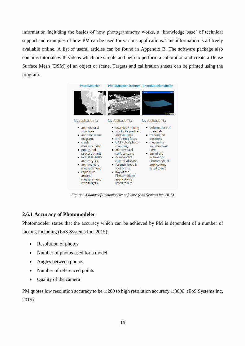
16
information including the basics of how photogrammetry works, a ‘knowledge base’ of technical
support and examples of how PM can be used for various applications. This information is all freely
available online. A list of useful articles can be found in Appendix B. The software package also
contains tutorials with videos which are simple and help to perform a calibration and create a Dense
Surface Mesh (DSM) of an object or scene. Targets and calibration sheets can be printed using the
program.
Figure 2.4 Range of Photomodeler software (EoS Systems Inc. 2015)
2.6.1 Accuracy of Photomodeler
Photomodeler states that the accuracy which can be achieved by PM is dependent of a number of
factors, including (EoS Systems Inc. 2015):
Resolution of photos
Number of photos used for a model
Angles between photos
Number of referenced points
Quality of the camera
PM quotes low resolution accuracy to be 1:200 to high resolution accuracy 1:8000. (EoS Systems Inc.
2015)
17
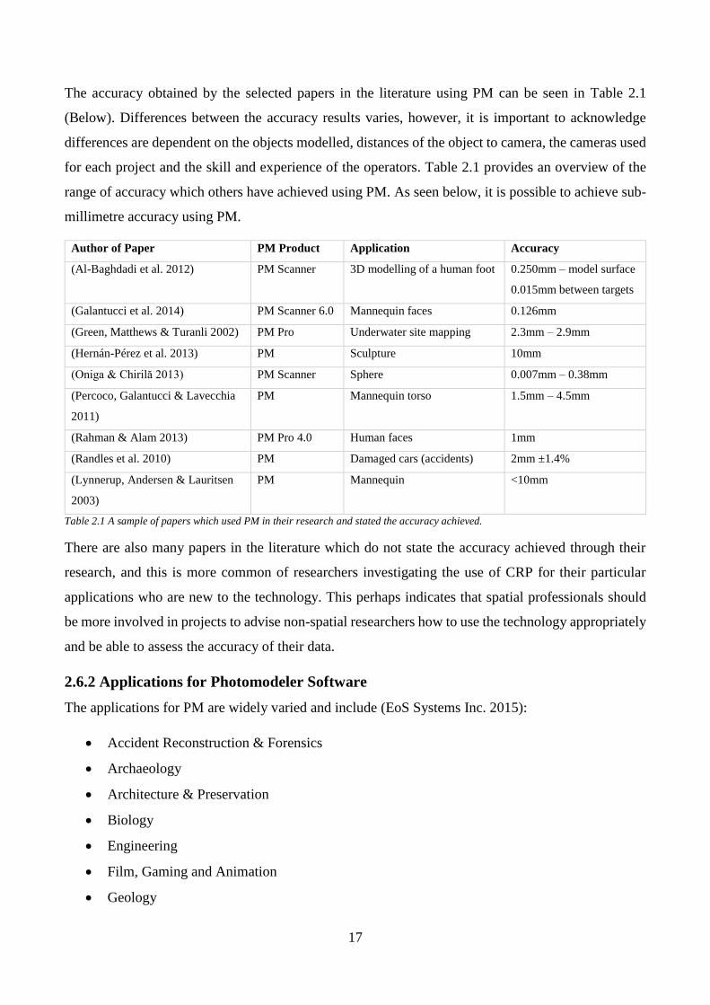
The accuracy obtained by the selected papers in the literature using PM can be seen in Table 2.1
(Below). Differences between the accuracy results varies, however, it is important to acknowledge
differences are dependent on the objects modelled, distances of the object to camera, the cameras used
for each project and the skill and experience of the operators. Table 2.1 provides an overview of the
range of accuracy which others have achieved using PM. As seen below, it is possible to achieve sub-
millimetre accuracy using PM.
Table 2.1 A sample of papers which used PM in their research and stated the accuracy achieved.
There are also many papers in the literature which do not state the accuracy achieved through their
research, and this is more common of researchers investigating the use of CRP for their particular
applications who are new to the technology. This perhaps indicates that spatial professionals should
be more involved in projects to advise non-spatial researchers how to use the technology appropriately
and be able to assess the accuracy of their data.
2.6.2 Applications for Photomodeler Software
The applications for PM are widely varied and include (EoS Systems Inc. 2015):
Accident Reconstruction & Forensics
Archaeology
Architecture & Preservation
Biology
Engineering
Film, Gaming and Animation
Geology
Author of Paper PM Product Application Accuracy
(Al-Baghdadi et al. 2012) PM Scanner 3D modelling of a human foot 0.250mm – model surface
0.015mm between targets
(Galantucci et al. 2014) PM Scanner 6.0 Mannequin faces 0.126mm
(Green, Matthews & Turanli 2002) PM Pro Underwater site mapping 2.3mm – 2.9mm
(Hernán-Pérez et al. 2013) PM Sculpture 10mm
(Oniga & Chirilă 2013) PM Scanner Sphere 0.007mm – 0.38mm
(Percoco, Galantucci & Lavecchia
2011)
PM Mannequin torso 1.5mm – 4.5mm
(Rahman & Alam 2013) PM Pro 4.0 Human faces 1mm
(Randles et al. 2010) PM Damaged cars (accidents) 2mm ±1.4%
(Lynnerup, Andersen & Lauritsen
2003)
PM Mannequin <10mm
18
Surveying
UAS / Drones
2.6.3 Advantages and Disadvantages of Photomodeler
Al-Baghdadi et al. (2011, p. 297) in their study of mapping the human foot chose to use PM Scanner
to create 3D surface models of the foot because of PM’s capability for DSMs and the ability to export
point clouds and triangulated meshes in a variety of formats for further analysis and manipulation. Al-
Baghdadi et al. (2011, pp. 298-9, 302) made a number of observations about how PM performed for
their study:
Black and white circular targets were captured by PM with greater accuracy than other colour
combinations.
A depth range was assigned to allow quicker processing and matching of the images to create
the DSM.
The foot needed to be painted with a matte red body paint to ensure uniform accuracy across
the DSM.
Individual toes were difficult to map due to being close together.
Galantucci et al. (2014, p. 288) remarks that the algorithm used for sub-pixel marking (recognising
points) in PM Scanner recognises these points by contrast. Points located laterally on a surface are
marked with an ellipse which results in a loss of precision. (Galantucci et al. 2014, p. 289) However,
for the application of clinical studies of body surfaces, PM provides a sufficient level of accuracy and
reliability. (Galantucci et al. 2014, p. 290)
Some of the points mentioned above are common remarks throughout the literature about CRP in
general and are not necessarily particular to PM software itself.
2.7 Summary
The literature review reveals that CRP has many advantages over other technologies in 3D mapping,
especially mapping the human body, fragile or inaccessible objects. The advantages include being non-
invasive, instantaneous, highly accurate, real world colour and texture, creation of a permanent record,
re-measurable and cost effective. Many of these characteristics are particular useful for human body
mapping.

19
While there are many advantages to using CRP for human body mapping, there are some common
problems in the literature, such as difficulty in modelling fine details, such as teeth and toes. Also,
where an object or body area touches a surface, like a table, holes can form in the 3D model. Modelling
hands or faces can produce inaccuracies due to movement of individual fingers or facial expressions.
Some researchers had difficulty combining data from CRP with other data capture techniques, such as
CT scans.
The calibration process is necessary for non-metric cameras designed for photography rather than
photogrammetry. The parameters which need to be determined by calibration include format size, focal
length, principal distance, principal point, radial distortion and decentring distortion. There are a few
different calibration techniques which can be used. The most appropriate for a low cost, off the shelf
digital cameras is self-calibration using a bundle adjustment to determine the parameters.
Researchers have produced accurate results using CRP and Photomodeler, including human body
mapping. In a sample of papers which used Photomodeler, accuracies varied between 0.007mm to
10mm across a wide variety of applications.

20
3.0 Chapter Three – Research Design and Methodology
3.1 Objectives
1. Camera Calibration
Determine the most appropriate calibration for the task, including the coded target type, number of
targets and discuss any differences between the two cameras.
2. Image Acquisition
Determine the optimal amount of targets to be used and configuration.
3. Data Processing and Creation of 3D Model
Analyse the level of difficulty and note any problems in the creation of the 3D model from the images.
4. Accuracy
Assess the accuracy of the 3D model using measurements taken by callipers and tape.
3.2 Implications of Research
It is intended that the outcome of this project will add to the knowledge base of the uses and
effectiveness of low cost CRP to model complex objects. Also, analysis and discussion of any
difficulties will be useful to determine how easy it is to create an accurate model. It may help students
and researchers in the future to determine if low cost CRP is suitable to apply to their particular task.
The impacts of this project are negligible, especially since the decision was made to use a model human
skull instead of a real one. If a real human skull was to be used, ethics would have needed to be
considered.
3.3 Equipment
3.3.1 Cameras
The cameras selected for the task are both Nikon S3700 (20.1 Megapixels), which are commonly
available and priced at $135.00 each at the time of purchase (May 2015).
3.3.2 Photogrammetry Software
The photogrammetry software selected is Photomodeler, priced at approximately $5000 (Al-Baghdadi
et al. 2011, p. 301) Photomodeler was selected as it is one of the cheaper, user friendly software
packages on the market and USQ was able to lend a licence for the duration of the project at no cost.

21
3.3.3 Targets
Targets are available as part of the Photomodeler Scanner software package to be printed and used.
3.3.4 Skull
It was originally proposed to use a real human skull for the project, but it was not possible to arrange
access. Alternatively, a high quality, cast model was used.
3.3.5 Callipers and Tape
A good quality Sidchrome digital calliper was purchased, 0-200mm, graduation: 0.01mm, model:
SCMT26116. A good quality 3m Stanley tape was also purchased.
3.3.6 Miscellaneous
A number of materials are available for use in the lab to create an appropriate background for the
photograph acquisition, such as black cardboard, frame, sticky tape etc. Also, other resources are
available, such as measuring tapes, scale and tripod. A painted photo frame was used for a control
target frame off campus.
3.4 Camera Calibration
A number of steps are required in the calibration process:
1. Select target type and size.
2. Choose method, single sheet or multi sheet calibration.
3. Decide position of camera and target sheet.
4. Capture a set of images.
5. Process the calibration using Photomodeler software.
6. Analyse the results.
3.4.1 Target Type and Size
The targets selected for the calibration are available to print in the Photomodeler software. To print
calibration sheet, go to File – Print Calibration Sheet(s)… This type of target is recommended for
small-scale projects, such as a car or foot print. (EoS Systems Inc. 2013, Ch.3) The target grid sheet,
known as a “Calibration Sheet” in the Photomodeler Tutorials, was printed to A3 size; a size which
covers the size of the skull. (See Image 3.1 below)

22
Image 3.1 Calibration grid from Photomodeler
3.4.2 Calibration Method
A single sheet calibration method was used, which is recommended for small scale projects. (EoS
Systems Inc. 2013, Ch.3) This involves photographing a single sheet (as pictured in Image 3.1) from
different angles and camera orientations, as recommended by Photomodeler. (EoS Systems Inc. 2013,
Ch.3) The Calibration Sheet was placed on the floor and fastened with sticky tape to remain flat and
prevent movement.
3.4.3 Camera and Calibration Grid Position
A total of twelve photographs were taken of the Calibration Sheet, see Figure 3.1 below. As seen from
Figure 3.1, eight photographs were taken from each side of the sheet, four in portrait orientation and
four in landscape orientation of the camera. An additional four were photographed from the corners,
in either portrait or landscape orientation. This procedure is recommended by Photomodeler. (EoS
Systems Inc. 2013, Ch.3)
There was a problem in the initial attempts of processing the calibration in PM at the USQ Laboratory,
due to the organisation of the calibration photos. If the photos for each calibration set are not saved in
separate folders, the calibration will experience problems which will only become evident when
attempting to process photos for the model in PM. It is important that directories for calibration sets
are kept separate and organised.
Figure 3.1 Configuration of target
camera positions and orientations.
23
3.5 Target Configuration
The placement of targets either around the object, on the object or both are an important consideration,
as it does affect the outcome of the photograph processing. In the Photomodeler tutorials (EoS Systems
Inc. 2013), there are examples of different objects being photographed. Some use only targets
surrounding the object, while others place targets on the object.
Numerous configurations were trialled, both with targets surrounding the skull and targets stuck onto
the skull. The success of the photo acquisition and DSM creation appears to be somewhat correlated
with the number of targets used, among other factors (discussed later). The target configuration aims
to orientate the image and provide a fixed point for the modelling.
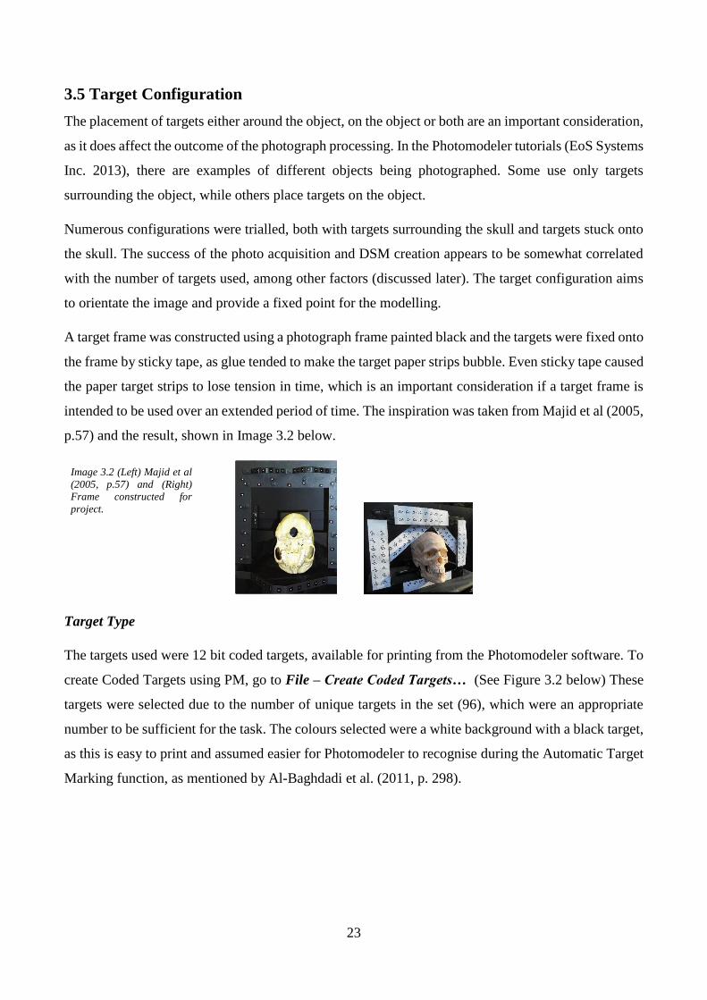
A target frame was constructed using a photograph frame painted black and the targets were fixed onto
the frame by sticky tape, as glue tended to make the target paper strips bubble. Even sticky tape caused
the paper target strips to lose tension in time, which is an important consideration if a target frame is
intended to be used over an extended period of time. The inspiration was taken from Majid et al (2005,
p.57) and the result, shown in Image 3.2 below.
Target Type
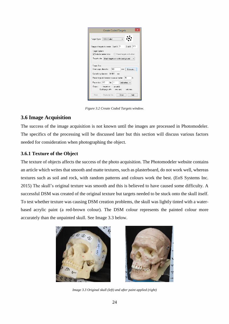
The targets used were 12 bit coded targets, available for printing from the Photomodeler software. To
create Coded Targets using PM, go to File – Create Coded Targets… (See Figure 3.2 below) These
targets were selected due to the number of unique targets in the set (96), which were an appropriate
number to be sufficient for the task. The colours selected were a white background with a black target,
as this is easy to print and assumed easier for Photomodeler to recognise during the Automatic Target
Marking function, as mentioned by Al-Baghdadi et al. (2011, p. 298).
Image 3.2 (Left) Majid et al
(2005, p.57) and (Right)
Frame constructed for
project.
24
Figure 3.2 Create Coded Targets window.
3.6 Image Acquisition
The success of the image acquisition is not known until the images are processed in Photomodeler.
The specifics of the processing will be discussed later but this section will discuss various factors
needed for consideration when photographing the object.
3.6.1 Texture of the Object
The texture of objects affects the success of the photo acquisition. The Photomodeler website contains
an article which writes that smooth and matte textures, such as plasterboard, do not work well, whereas
textures such as soil and rock, with random patterns and colours work the best. (EoS Systems Inc.
2015) The skull’s original texture was smooth and this is believed to have caused some difficulty. A
successful DSM was created of the original texture but targets needed to be stuck onto the skull itself.
To test whether texture was causing DSM creation problems, the skull was lightly tinted with a water-
based acrylic paint (a red-brown colour). The DSM colour represents the painted colour more
accurately than the unpainted skull. See Image 3.3 below.
Image 3.3 Original skull (left) and after paint applied (right)

25
Other methods of introducing texture to the skull were also tried, such as dusting with talcum powder,
dirt and foundation powder make-up, but these were unsuccessful in creating a DSM. Powder and
paint are recommended by Photomodeler (EoS Systems Inc. 2015) and Al-Baghdadi et al. (2011) also
used paint for better results of creating DSMs of feet. Real bone textures, especially weathered or old
specimens, would perhaps perform better due to having a more random surface texture.
3.6.2 Lighting
The lighting was considered as a possible cause of difficulties, as Alshadli, Duaa et al. (2013) had
problems with glass and Cevidanes et al. (2010) with the iris of the eye. PM also recommends
consistent lighting across photos to improve textures. (EoS Systems Inc. 2013, Ch.2-3) The aim of
lighting is to decrease shadow and contrast between the image and the background to ultimately
improve DSM results. The problem with photographing indoors is that the lighting is likely to be dull.
Using lights often adds shadow to the photos and it proved difficult to press the button on the camera
to take the photo without making shadows on the skull. Photographing in natural light appears to
produce better quality, evenly coloured and realistic textured photographs without shadow.
3.6.3 Background
The background of the object is also important. When a background is not used, there are many
unwanted points and noise captured in the photo. When the skull was photographed without a
background, the Automatic Target Marking function in PM would mistakenly identify texture in the
background as a target, especially if the image capture was outside (with trees and randomly textured
earth in the background). A black background was used so that light would not be reflected and would
not appear shiny, the skull would contrast with the background and the targets would be distinctive. A
black background was used in CRP image capture of the skulls for the Malaysian Craniofacial
Database. (Majid 2005).
3.6.4 Camera Position and Angles
If the camera is placed at an acute angle, the targets will not be recognised by the Automatic Target
Marking process, which occurred in some of the unsuccessful attempts. Keeping the photos at a
moderate angle yields better results. Also, positioning the camera so that the control frame and skull
are contained in a large portion of the photo improves the result. Figure 3.3 below shows the different
camera positions (represented by blue squares) to capture the images of the skull.

26
3.6.5 Camera Settings
Another issue to consider is a particular camera’s default settings, which may come into effect each
time the camera is switched on or off. For this project, each time the camera was used the flash was
switched off and the zoom checked to ensure it was fully zoomed out, as the flash in particular
automatically is enabled each time the camera is powered on and off.
3.7 Processing
Appendix D outlines the steps taken to create the DSM model. This section will detail specific selected
settings used for discussion.
3.7.1 Uploading Photos
Photos can be uploaded to Photomodeler and automatically oriented using the step by step process. It
is important not to orientate, crop, or modify the photos in any way otherwise the project will not
process. (EoS Systems Inc. 2013, Ch.5) For reasons unknown at this stage, the Red camera used to
capture the photos for the model sometimes orientated landscape photos 90° and when modified to the
correct orientation before uploading to PM, the processing was unsuccessful.
3.7.2 Automatic Target Marking
The Automatic Target Marking function in PM recognises targets automatically in each photo. This
process is able to be performed manually (EoS Systems Inc. 2013, Ch.5), however, the automatic
function saves a significant amount of time, especially if there are many targets. Figure 3.4 below
shows the various settings and options which can be selected for the operation.
Figure 3.3 Skull showing location of camera stations

27
Figure 3.4 Automatic Target Marking options.
Two issues occurred with this operation. Firstly, when targets are printed for use, they are unique and
numbered accordingly, for example, in 12-bit there are 96 targets. If a few sets of targets are printed,
it is important not to use two identical targets in the photo, as the photos will not be oriented and
automatic targeting will not work. Secondly, targets may not be identified if there is too much shadow
in the photo or if there are objects in the photo which may be confused with a target.
3.7.3 Processing
Default options were accepted and the project was processed. See Figure 3.5 below.
Figure 3.5 Processing options.
A report can be saved as a text file which contains useful data which indicates the quality of the
processing outcome. Some useful indicators of quality contained in this report are listed in Table 3.1.
(See Appendix C for full report) Tables can also be generated through the View menu, which can list
a more comprehensive list of parameters and results.
28
Quality Indicator Result Comment
Number of photos oriented 9 Good result, all photos have been oriented
Bad Photos 0
Weak Photos 0
OK Photos 9 Good results, all photos are acceptable
Average Photo Point Coverage 50% 80% + is best
Point Marking Residuals
Overall RMS 0.819 pixels Satisfactory result, RMS <1.0
Maximum RMS 1.667 pixels
Minimum RMS 0.324 pixels
Table 3.1 Indicators of quality in the processing report.
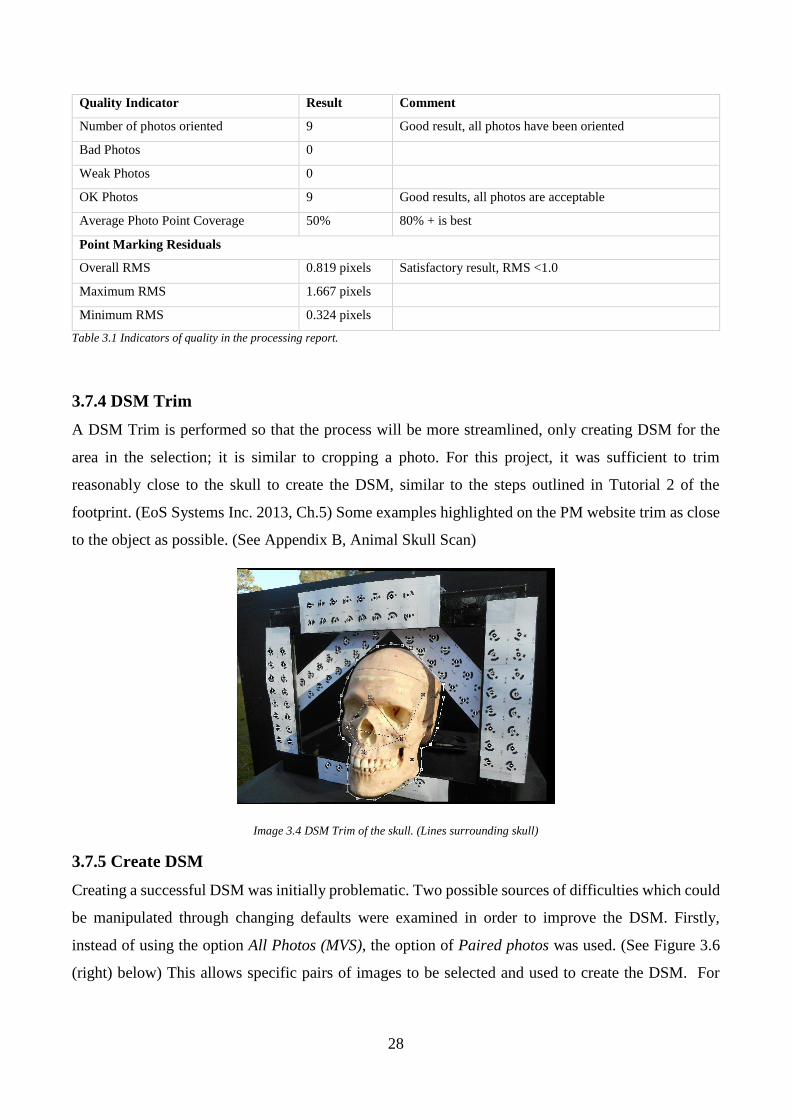
3.7.4 DSM Trim
A DSM Trim is performed so that the process will be more streamlined, only creating DSM for the
area in the selection; it is similar to cropping a photo. For this project, it was sufficient to trim
reasonably close to the skull to create the DSM, similar to the steps outlined in Tutorial 2 of the
footprint. (EoS Systems Inc. 2013, Ch.5) Some examples highlighted on the PM website trim as close
to the object as possible. (See Appendix B, Animal Skull Scan)
Image 3.4 DSM Trim of the skull. (Lines surrounding skull)
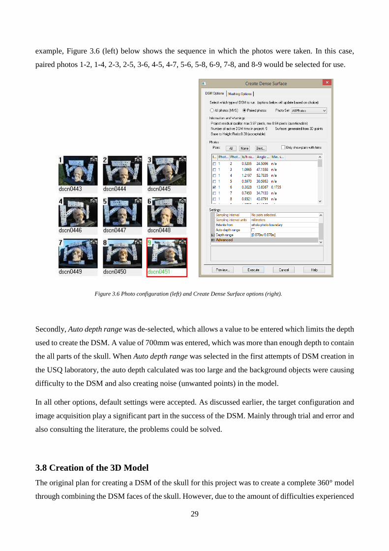
3.7.5 Create DSM
Creating a successful DSM was initially problematic. Two possible sources of difficulties which could
be manipulated through changing defaults were examined in order to improve the DSM. Firstly,
instead of using the option All Photos (MVS), the option of Paired photos was used. (See Figure 3.6
(right) below) This allows specific pairs of images to be selected and used to create the DSM. For
29
example, Figure 3.6 (left) below shows the sequence in which the photos were taken. In this case,
paired photos 1-2, 1-4, 2-3, 2-5, 3-6, 4-5, 4-7, 5-6, 5-8, 6-9, 7-8, and 8-9 would be selected for use.
Secondly, Auto depth range was de-selected, which allows a value to be entered which limits the depth
used to create the DSM. A value of 700mm was entered, which was more than enough depth to contain
the all parts of the skull. When Auto depth range was selected in the first attempts of DSM creation in
the USQ laboratory, the auto depth calculated was too large and the background objects were causing
difficulty to the DSM and also creating noise (unwanted points) in the model.
In all other options, default settings were accepted. As discussed earlier, the target configuration and
image acquisition play a significant part in the success of the DSM. Mainly through trial and error and
also consulting the literature, the problems could be solved.
3.8 Creation of the 3D Model
The original plan for creating a DSM of the skull for this project was to create a complete 360° model
through combining the DSM faces of the skull. However, due to the amount of difficulties experienced
Figure 3.6 Photo configuration (left) and Create Dense Surface options (right).

30
during the project, which impacted on time, a single frontal face DSM was created. The single face is
still able to be used for taking measurements and the accuracy assessed, which satisfies the project
objectives. A drawback of having a single face is that the accuracy and ease of being able to combine
different DSM faces of the skull cannot be assessed.
In earlier attempts of creating a DSM, particularly at the USQ Laboratory, there were a large number
of unwanted points or noise in the DSM. Manual deletion of the unwanted points is the only option to
remove them and this took a significant amount of time, which is the reason further attempts of
improving the DSM were pursued. The final DSM using the tinted skull photographed in natural light
had minimal amounts of unwanted points.
The DSM and Points could be exported into a number of different file types, see Figure 3.7. The final
DSM was exported to a DXF file type for use in AutoCAD. A number of options can be used to control
what layers or objects are exported as part of the DXF file. In this case, the point mesh, DSM, targets
and drawn lines (used for comparing measurements, discussed later) were exported successfully.
Using AutoCAD in 3D Modelling was tiresome due to the limitations of the computer used. The
program was slow and became unresponsive a number of times, especially when zooming, rotating or
moving the model or attempting to select large areas of points. The model window in PM proved easier
and quicker to use for taking measurements and showing a photo-realistic DSM.
Figure 3.7 Export options (left) and screen shot of resulting DXF file in AutoCAD
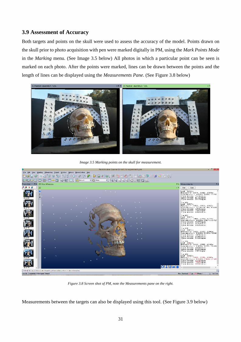
31
3.9 Assessment of Accuracy
Both targets and points on the skull were used to assess the accuracy of the model. Points drawn on
the skull prior to photo acquisition with pen were marked digitally in PM, using the Mark Points Mode
in the Marking menu. (See Image 3.5 below) All photos in which a particular point can be seen is
marked on each photo. After the points were marked, lines can be drawn between the points and the
length of lines can be displayed using the Measurements Pane. (See Figure 3.8 below)
Image 3.5 Marking points on the skull for measurement.
Figure 3.8 Screen shot of PM, note the Measurements pane on the right.
Measurements between the targets can also be displayed using this tool. (See Figure 3.9 below)
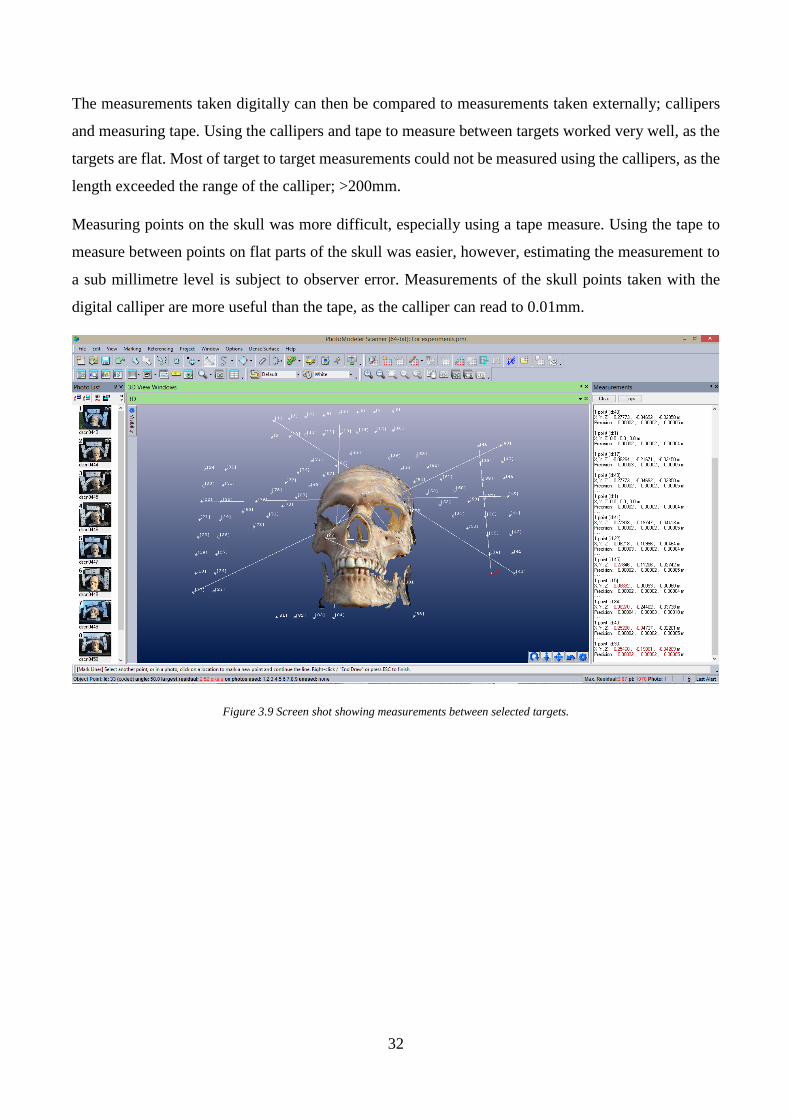
32
The measurements taken digitally can then be compared to measurements taken externally; callipers
and measuring tape. Using the callipers and tape to measure between targets worked very well, as the
targets are flat. Most of target to target measurements could not be measured using the callipers, as the
length exceeded the range of the calliper; >200mm.
Measuring points on the skull was more difficult, especially using a tape measure. Using the tape to
measure between points on flat parts of the skull was easier, however, estimating the measurement to
a sub millimetre level is subject to observer error. Measurements of the skull points taken with the
digital calliper are more useful than the tape, as the calliper can read to 0.01mm.
Figure 3.9 Screen shot showing measurements between selected targets.

33
4.0 Chapter Four – Results and Discussion
4.1 Camera Calibration
Three calibrations (3 sets per camera) were performed using three sets of data to attempt to improve
the calibration results, see Table 4.1. However, the best calibration (lowest maximum residual) was
the first calibration performed in the USQ Laboratory. (See Table 4.2 for full results)
Calibration ID Comments
Red Set A
Blue Set A
The first calibration sets attempted at the USQ Photogrammetry Lab
Red Set B
Blue Set B
Calibration performed off campus. Camera settings adjusted and stronger lighting adopted.
Red Set C
Blue Set C
Calibration performed off campus. Camera settings adjusted and calibration grid set up closer
to camera to improve photograph coverage with lighting adjustments.
Table 4.1 Calibration sets completed and comments.
Figure 4.1 Overall RMS for all three sets.
Figure 4.2 Maximum residuals for all three sets.

34
4.1.1 Results of Calibration
Calibration Set Focal Lth Xp Yp Fw Fh K1 K2 K3 P1 P2 Overall RMS Max Residual
Red Set A 1 4.80835500 3.31388800 2.42188200 6.48033000 4.86000000 0.00026690 0.00001061 0.00000000 -0.00117800 -0.00004575 0.390 0.983
Red Set A 2 4.79843800 3.30672200 2.42120800 6.47820300 4.86000000 0.00043960 0.00000000 0.00000000 -0.00107500 -0.00010890 0.400 1.285
Red Set A 3 4.79071600 3.29069800 2.43371200 6.47953600 4.86000000 0.00039550 0.00003105 0.00000000 -0.00075840 0.00012950 0.372 1.216
Blue Set A 1 4.85448000 3.34207300 2.43645400 6.48285000 4.86000000 0.00042980 -0.00005714 0.00000000 -0.00176300 0.00023960 0.416 1.214
Blue Set A 2 4.84141000 3.32898600 2.44414600 6.48173800 4.86000000 0.00023880 0.00000000 0.00000000 -0.00148700 0.00034540 0.410 1.557
Blue Set A 3 4.83674000 3.32833500 2.44518900 6.48078700 4.86000000 0.00037640 -0.00001739 0.00000000 -0.00150000 0.00037090 0.426 1.503
Red Set B 1 4.81893200 3.31501300 2.42588600 6.48541100 4.86000000 0.00089370 -0.00015700 0.00000000 -0.00103700 0.00000000 0.388 1.469
Red Set B 2 4.81756900 3.30777800 2.42346700 6.47852700 4.86000000 0.00214700 -0.00054510 0.00000000 0.00101800 0.00000000 0.665 3.442
Red Set B 3 4.81632700 3.31104700 2.43134900 6.48164700 4.86000000 0.00124000 -0.00024660 0.00000000 -0.00102700 0.00015140 0.370 1.404
Blue Set B 1 4.86034500 3.35882700 2.44206100 6.48086600 4.86000000 0.00178300 -0.00053790 0.00000000 -0.00196700 0.00033560 0.388 1.385
Blue Set B 2 4.86173700 3.32426600 2.43927200 6.48128200 4.86000000 0.00176200 -0.00057590 0.00000000 -0.00127200 0.00037350 0.368 1.097
Blue Set B 3 4.85623800 3.33053400 2.44701800 6.48155100 4.86000000 0.00182500 -0.00045190 0.00000000 -0.00150300 0.00046130 0.495 2.667
Red Set C 1 4.80913500 3.31721700 2.40963900 6.47650500 4.86000000 0.00055980 -0.00001529 0.00000000 -0.00134100 -0.00025130 0.463 1.509
Red Set C 2 4.80136000 3.28493700 2.42092100 6.47442800 4.86000000 0.00053720 -0.00001928 0.00000000 -0.00073040 -0.00014080 0.448 1.264
Red Set C 3 4.80185100 3.30448100 2.41131200 6.47408900 4.86000000 0.00052650 -0.00001570 0.00000000 -0.00114100 -0.00032120 0.482 1.747
Blue Set C 1 4.83451900 3.32712600 2.43492100 6.47441700 4.86000000 0.00023230 -0.00002782 0.00000000 -0.00158400 0.00019410 0.485 2.002
Blue Set C 2 4.84708300 3.33801200 2.42047200 6.47564400 4.86000000 0.00025480 -0.00002184 0.00000000 -0.00180600 -0.00004686 0.460 1.356
Blue Set C 3 4.83597300 3.32679500 2.43544000 6.47601900 4.86000000 0.00022310 -0.00003413 0.00000000 -0.00160700 0.00020020 0.559 1.884
Table 4.2 Camera calibration results showing parameters, Root Mean Squared (RMS) and Maximum Residual

35
4.1.2 Discussion of Calibration Results
A number of difficulties were encountered during the calibration phase of the project, which is the
reason a number of calibrations were performed to examine if the calibration results could be
improved. The best result was the first calibration set (Red Set A 1), see Table 4.2 above, which was
performed in the USQ Laboratory. As shown in Figure 4.1 and Figure 4.2, Red Set B 2 produced a
spike in results, but Set A and C have closer similarity. The conditions in the laboratory differed to
those off campus in the following ways:
Lighting
Lights (LED and halogen) were used off campus, which created some shadowing of the tripod and
camera which was controlled where possible (e.g. placing the camera so that shadows did not fall
across the calibration sheet). This could have created a poorer camera position geometry as the
shadows were the concern, not the camera position. The lighting in the Laboratory was duller but did
not cast shadows.
Percentage of calibration sheet in photo
The percentage of the calibration sheet in the photo was less in the off campus calibrations than on
campus. The reason for this is that a larger tripod was used off campus; the smaller tripod on campus
allowed the camera to be set up closer to the calibration sheet. A small table was used to attempt to
improve the distance between the camera and calibration sheet, however, the tripod continued to cause
problems due to the size. It also increased the risk of bumping the table causing the calibration sheet
to move.

36
4.2 Photograph Capture and Processing
The final model was produced off campus after tinting the skull with acrylic paint. The following
(Figure 4.3 and Figure 4.4) are images from PM of the 3D model represented in different ways:
Figure 4.4 DSM with points coloured by depth (top left), DSM points coloured by photo texture overlaid with point cloud (top right),
DSM shown as triangulated mesh (bottom left) and DSM showing close correlation with point cloud underneath (bottom right).
Figure 4.3 DSM coloured with photo texture (left) & DSM using single texture with points coloured with photo texture (right).
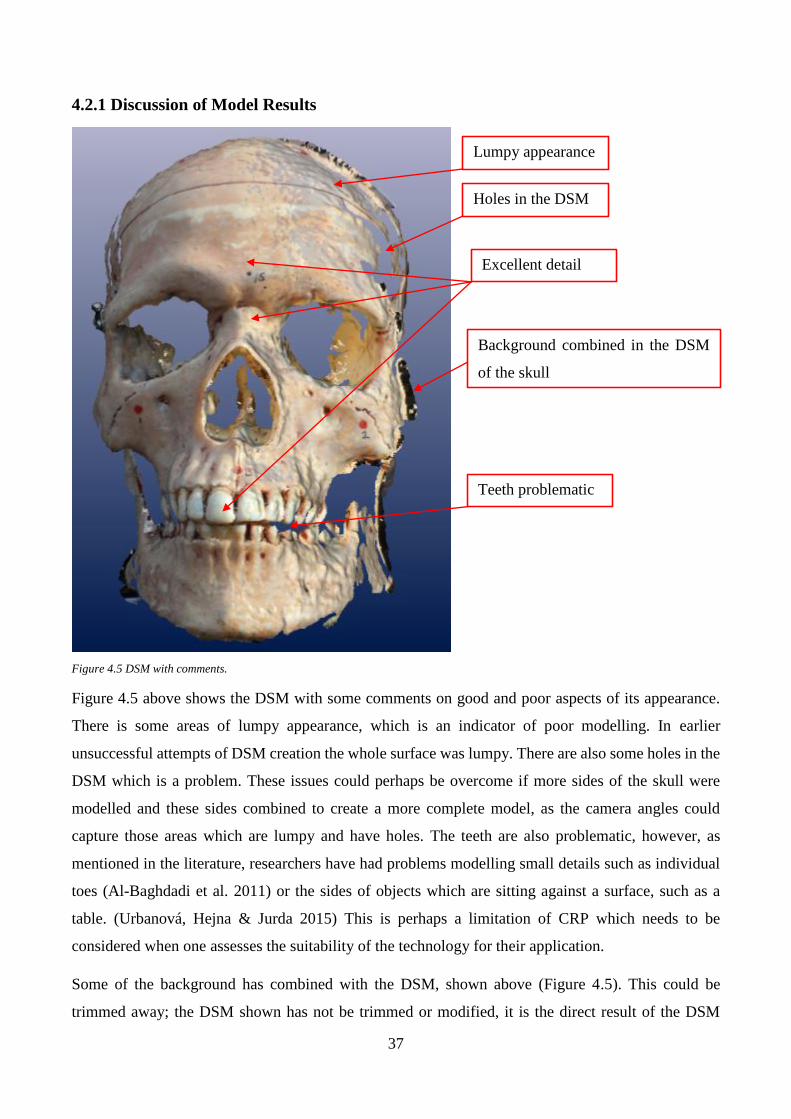
37
4.2.1 Discussion of Model Results
Figure 4.5 DSM with comments.
Figure 4.5 above shows the DSM with some comments on good and poor aspects of its appearance.
There is some areas of lumpy appearance, which is an indicator of poor modelling. In earlier
unsuccessful attempts of DSM creation the whole surface was lumpy. There are also some holes in the
DSM which is a problem. These issues could perhaps be overcome if more sides of the skull were
modelled and these sides combined to create a more complete model, as the camera angles could
capture those areas which are lumpy and have holes. The teeth are also problematic, however, as
mentioned in the literature, researchers have had problems modelling small details such as individual
toes (Al-Baghdadi et al. 2011) or the sides of objects which are sitting against a surface, such as a
table. (Urbanová, Hejna & Jurda 2015) This is perhaps a limitation of CRP which needs to be
considered when one assesses the suitability of the technology for their application.
Some of the background has combined with the DSM, shown above (Figure 4.5). This could be
trimmed away; the DSM shown has not be trimmed or modified, it is the direct result of the DSM
Lumpy appearance
Holes in the DSM
Teeth problematic
Background combined in the DSM
of the skull
Excellent detail
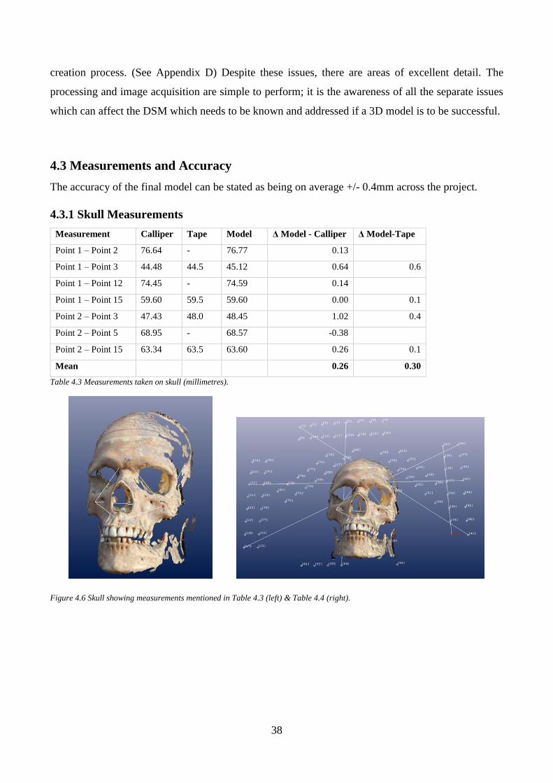
38
creation process. (See Appendix D) Despite these issues, there are areas of excellent detail. The
processing and image acquisition are simple to perform; it is the awareness of all the separate issues
which can affect the DSM which needs to be known and addressed if a 3D model is to be successful.
4.3 Measurements and Accuracy
The accuracy of the final model can be stated as being on average +/- 0.4mm across the project.
4.3.1 Skull Measurements
Measurement Calliper Tape Model Δ Model - Calliper Δ Model-Tape
Point 1 – Point 2 76.64 - 76.77 0.13
Point 1 – Point 3 44.48 44.5 45.12 0.64 0.6
Point 1 – Point 12 74.45 - 74.59 0.14
Point 1 – Point 15 59.60 59.5 59.60 0.00 0.1
Point 2 – Point 3 47.43 48.0 48.45 1.02 0.4
Point 2 – Point 5 68.95 - 68.57 -0.38
Point 2 – Point 15 63.34 63.5 63.60 0.26 0.1
Mean 0.26 0.30
Table 4.3 Measurements taken on skull (millimetres).
Figure 4.6 Skull showing measurements mentioned in Table 4.3 (left) & Table 4.4 (right).
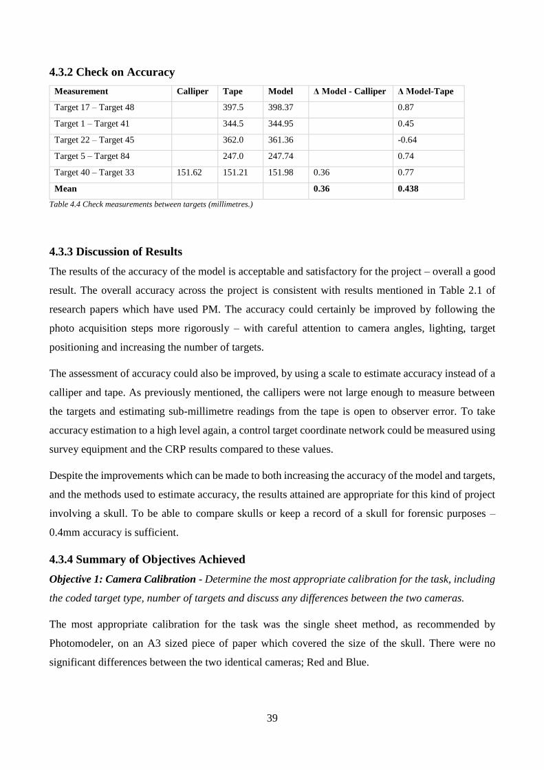
39
4.3.2 Check on Accuracy
Measurement Calliper Tape Model Δ Model - Calliper Δ Model-Tape
Target 17 – Target 48 397.5 398.37 0.87
Target 1 – Target 41 344.5 344.95 0.45
Target 22 – Target 45 362.0 361.36 -0.64
Target 5 – Target 84 247.0 247.74 0.74
Target 40 – Target 33 151.62 151.21 151.98 0.36 0.77
Mean 0.36 0.438
Table 4.4 Check measurements between targets (millimetres.)
4.3.3 Discussion of Results
The results of the accuracy of the model is acceptable and satisfactory for the project – overall a good
result. The overall accuracy across the project is consistent with results mentioned in Table 2.1 of
research papers which have used PM. The accuracy could certainly be improved by following the
photo acquisition steps more rigorously – with careful attention to camera angles, lighting, target
positioning and increasing the number of targets.
The assessment of accuracy could also be improved, by using a scale to estimate accuracy instead of a
calliper and tape. As previously mentioned, the callipers were not large enough to measure between
the targets and estimating sub-millimetre readings from the tape is open to observer error. To take
accuracy estimation to a high level again, a control target coordinate network could be measured using
survey equipment and the CRP results compared to these values.
Despite the improvements which can be made to both increasing the accuracy of the model and targets,
and the methods used to estimate accuracy, the results attained are appropriate for this kind of project
involving a skull. To be able to compare skulls or keep a record of a skull for forensic purposes –
0.4mm accuracy is sufficient.
4.3.4 Summary of Objectives Achieved
Objective 1: Camera Calibration - Determine the most appropriate calibration for the task, including
the coded target type, number of targets and discuss any differences between the two cameras.
The most appropriate calibration for the task was the single sheet method, as recommended by
Photomodeler, on an A3 sized piece of paper which covered the size of the skull. There were no
significant differences between the two identical cameras; Red and Blue.
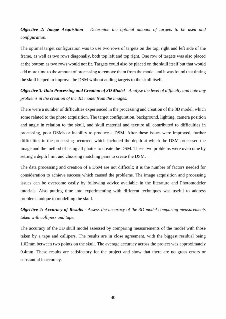
40
Objective 2: Image Acquisition - Determine the optimal amount of targets to be used and
configuration.
The optimal target configuration was to use two rows of targets on the top, right and left side of the
frame, as well as two rows diagonally, both top left and top right. One row of targets was also placed
at the bottom as two rows would not fit. Targets could also be placed on the skull itself but that would
add more time to the amount of processing to remove them from the model and it was found that tinting
the skull helped to improve the DSM without adding targets to the skull itself.
Objective 3: Data Processing and Creation of 3D Model - Analyse the level of difficulty and note any
problems in the creation of the 3D model from the images.
There were a number of difficulties experienced in the processing and creation of the 3D model, which
some related to the photo acquisition. The target configuration, background, lighting, camera position
and angle in relation to the skull, and skull material and texture all contributed to difficulties in
processing, poor DSMs or inability to produce a DSM. After these issues were improved, further
difficulties in the processing occurred, which included the depth at which the DSM processed the
image and the method of using all photos to create the DSM. These two problems were overcome by
setting a depth limit and choosing matching pairs to create the DSM.
The data processing and creation of a DSM are not difficult; it is the number of factors needed for
consideration to achieve success which caused the problems. The image acquisition and processing
issues can be overcome easily by following advice available in the literature and Photomodeler
tutorials. Also putting time into experimenting with different techniques was useful to address
problems unique to modelling the skull.
Objective 4: Accuracy of Results - Assess the accuracy of the 3D model comparing measurements
taken with callipers and tape.
The accuracy of the 3D skull model assessed by comparing measurements of the model with those
taken by a tape and callipers. The results are in close agreement, with the biggest residual being
1.02mm between two points on the skull. The average accuracy across the project was approximately
0.4mm. These results are satisfactory for the project and show that there are no gross errors or
substantial inaccuracy.
41
5.0 Chapter Five - Conclusions
5.1 Introduction
There is much literature written on the benefits of using CRP for a number of applications, including
human body mapping. While there is wide agreement that CRP is a useful tool which has advantages
over other technologies there are also a number of issues which can occur in the process of creating a
3D model. CRP may not be suitable for some applications and to achieve success may take a number
of trials, depending on the environment and conditions.
5.2 Conclusions
The number of variables and aspects to “get right” were underestimated initially; there are many
opportunities for “things to go wrong” and affect the DSM creation in PM. Solving those problems
took a significant amount of time, mainly through trial and error, which decreased the amount of time
in the project time frame to be able to work on other tasks, such as creating a complete model. However,
practise is a good way to learn about what kind of issues will affect a project, as using a different object
may have raised different issues.
The difficulty in using a tape in particular to measure points on a curved object, such as the skull, was
overlooked. A better method for comparing a highly accurate method of measurement like CRP would
have been more appropriate, such as using a scale bar in the photos to estimate accuracy. The callipers
worked well on the skull but were not long enough to measure between the targets on the control frame.
Photomodeler performed well and was relatively simple to learn to use the basics of the program. There
was no prior knowledge of using Photomodeler and the tutorials provided with the product are very
useful and assisted in learning. There are many more functions and useful tools in Photomodeler than
are discussed in this project. More time dedicated to learning Photomodeler would have been better.
All things considered, the accuracy attained and methods used in this project are appropriate for
modelling an object such as a skull. The project is useful for detailing and emphasising good practice
and stressing that following steps thoroughly is important in producing successful, quality results. All
of the project objectives were successfully completed:
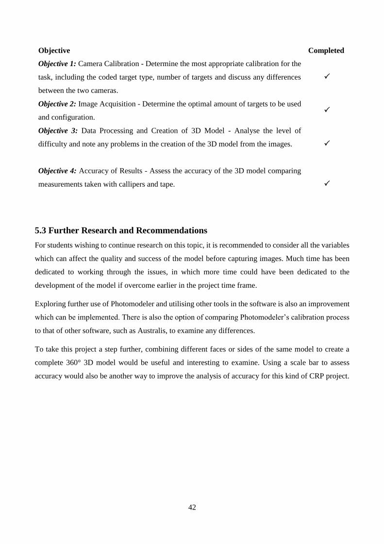
42
Objective Completed
Objective 1: Camera Calibration - Determine the most appropriate calibration for the
task, including the coded target type, number of targets and discuss any differences
between the two cameras.
Objective 2: Image Acquisition - Determine the optimal amount of targets to be used
and configuration.
Objective 3: Data Processing and Creation of 3D Model - Analyse the level of
difficulty and note any problems in the creation of the 3D model from the images.
Objective 4: Accuracy of Results - Assess the accuracy of the 3D model comparing
measurements taken with callipers and tape.
5.3 Further Research and Recommendations
For students wishing to continue research on this topic, it is recommended to consider all the variables
which can affect the quality and success of the model before capturing images. Much time has been
dedicated to working through the issues, in which more time could have been dedicated to the
development of the model if overcome earlier in the project time frame.
Exploring further use of Photomodeler and utilising other tools in the software is also an improvement
which can be implemented. There is also the option of comparing Photomodeler’s calibration process
to that of other software, such as Australis, to examine any differences.
To take this project a step further, combining different faces or sides of the same model to create a
complete 360° 3D model would be useful and interesting to examine. Using a scale bar to assess
accuracy would also be another way to improve the analysis of accuracy for this kind of CRP project.
43
References
Al-Baghdadi, JA, Chong, AK, McDougall, K & Alshadli, D 2012, 'An investigation of the 3-dimensional
surface capture techniques of the human foot', in International Workshop on Geoinformation Advances 2012:
proceedings of theInternational Workshop on Geoinformation Advances 2012, AA Rahman, et al. (eds.),
Universiti Teknologi Malaysia, Johor Bahru, Malaysia, pp. 26-47, <http://eprints.usq.edu.au/22494/>.
Al-Baghdadi, JAA, Chong, AK & Alshadli, D 2013, 'Compensation of measurement errors caused by glass
refraction for photogrammetric plantar surface mapping', Photogrammetric Record, vol. 28, no. 143, pp. 261-
75.
Al-Baghdadi, JAA, Chong, AK, McDougall, K, Alshadli, D, Milburn, P & Newsham-West, R 2011, 'A dense
surface modelling technique for foot surface imaging', in 2011 Surveying and Spatial Sciences Conference:
Innovation in Action: Working Smarter (SSSC 2011): proceedings of the2011 Surveying and Spatial Sciences
Conference: Innovation in Action: Working Smarter (SSSC 2011) Scion, Wellington, New Zealand, pp. 295-
302, <http://eprints.usq.edu.au/20586/>.
Alshadli, D, Chong, AK, Newsham-West, R, Al-Baghdadi, JAA, Milburn, P & McDougall, K 2013, 'A
comparison between static and dynamic foot mobility magnitude measures', in International Conference on
Biomechanics in Sports: proceedings of theInternational Conference on Biomechanics in Sports, H Toby (ed.),
National Taiwan Normal University, Taipei, <http://eprints.usq.edu.au/25083/>.
Alshadli, D, Chong, AK, McDougall, K, Al-Baghdadi, J, Milburn, P & & Newsham-West, R 2013, 'Reliability
of a high accuracy image-based system for 3D modelling of the medial longitudinal arch during gait', in
International Workshop on Geoinformation Advances 2012: proceedings of theInternational Workshop on
Geoinformation Advances 2012, AA Rahman, et al. (eds.), Springer-Verlag, Johor, Malaysia, pp. 85-101,
<http://eprints.usq.edu.au/23440/>.
Ayoub, AF, Xiao, Y, Khambay, B, Siebert, JP & Hadley, D 2007, 'Towards building a photo-realistic virtual
human face for craniomaxillofacial diagnosis and treatment planning', International Journal of Oral and
Maxillofacial Surgery, vol. 36, no. 5, pp. 423-8, Scopus.
Cevidanes, LHC, Motta, A, Proffit, WR, Ackerman, JL & Styner, M 2010, 'Cranial base superimposition for 3-
dimensional evaluation of soft-tissue changes', American Journal of Orthodontics and Dentofacial Orthopedics,
vol. 137, no. 4 SUPPL., pp. S120-S9, Scopus.
Chong, AK-F 2006, 'Photogrammetry for digital hand surface capture in swimming performance study', in
ISPRS Commission V Symposium: Image Engineering and Vision Metrology: proceedings of theISPRS
Commission V Symposium: Image Engineering and Vision Metrology, HG Maas & D Schneider (eds.),
International Society for Photogrammetry and Remote Sensing (ISPRS), Dresden, Germany, pp. 74-7,
<http://eprints.usq.edu.au/7371/>.
Chong, AK 2002, 'A Rigorous Technique for Forensic Measurement of Surveillance Video Footage',
Photogrammetric Engineering & Remote Sensing, vol. 68, no. 7, pp. 753-9.
Chong, AK 2011, 'Low-cost compact cameras: A medical application in CMT disease monitoring',
Photogrammetric Record, vol. 26, no. 134, pp. 263-73, Scopus.

44
Chong, AK, Milburn, P, Newsham-West, R & ter Voert, M 2009, 'High-accuracy photogrammetric technique
for human spine measurement', Photogrammetric Record, vol. 24, no. 127, pp. 264-79, Scopus.
Chong, AK, Majid, ZB, Ahmad, AB, Setan, HB & Samsudin, ABR 2004, 'The use of a national craniofacial
database', New Zealand Surveyor, no. 294, pp. 15-8.
Dellepiane, M, Dell'Unto, N, Callieri, M, Lindgren, S & Scopigno, R 2013, 'Archeological excavation
monitoring using dense stereo matching techniques', Journal of Cultural Heritage, vol. 14, no. 3, pp. 201-10,
Scopus.
EoS Systems Inc. 2013, User's Manual of PhotoModeler Scanner 2013, EoS Systems Inc.,.
EoS Systems Inc. 2015, Photomodeler, EoS Systems Inc., <http://www.photomodeler.com/index.html>.
Fryer, J 2001, Close range photogrammetry and machine vision, [New ed.]. edn, Whittles, Caithness.
Fryer, J, Mitchell, H & Chandler, JH 2007, Applications of 3D measurement from images, Whittles, Dunbeath.
Low cost 3D face scanning based on landmarks and photogrammetry: A new tool for a surface diagnosis in
orthodontics, Key Subjects <http://www.scopus.com/inward/record.url?eid=2-s2.0-
84867284478&partnerID=40&md5=163b2f4a867315ca394cde88cf8e27c3>.
Galantucci, LM, Lavecchia, F, Percoco, G & Raspatelli, S 2014, 'New method to calibrate and validate a high-
resolution 3D scanner, based on photogrammetry', Precision Engineering, vol. 38, no. 2, pp. 279-91, Scopus.
Green, J, Matthews, S & Turanli, T 2002, 'Underwater archaeological surveying using PhotoModeler,
VirtualMapper: different applications for different problems', The International Journal of Nautical
Archaeology, vol. 31, no. 2, pp. 283-92.
Guarnieri, A, Pirotti, F & Vettore, A 2010, 'Cultural heritage interactive 3D models on the web: An approach
using open source and free software', Journal of Cultural Heritage, vol. 11, no. 3, pp. 350-3, Scopus.
Hassan, MFA, Ma'Arof, I & Samad, AM 2014, 'Assessment of camera calibration towards accuracy
requirement', in Proceedings - 2014 IEEE 10th International Colloquium on Signal Processing and Its
Applications, CSPA 2014: proceedings of theProceedings - 2014 IEEE 10th International Colloquium on Signal
Processing and Its Applications, CSPA 2014 pp. 123-8, <http://www.scopus.com/inward/record.url?eid=2-s2.0-
84901685922&partnerID=40&md5=b9e47f1fe42d02f6431a2a6b3ba8848e>.
Hernán-Pérez, AS, Domínguez, MG, González, CR & Martín, AP 2013, 'Using iphone camera in photomodeler
for the 3D survey of a sculpture as practice for architecturés students', in Procedia Computer Science:
proceedings of theProcedia Computer Science pp. 345-7, <http://www.scopus.com/inward/record.url?eid=2-
s2.0-84890773624&partnerID=40&md5=14faa6e06c5fb4cba8de98d58c62a1c2>.
Hoevenaren, IA, Maal, TJJ, Krikken, E, De Haan, AFJ, Bergé, SJ & Ulrich, DJO 2015, 'Development of a three-
dimensional hand model using 3D stereophotogrammetry: Evaluation of landmark reproducibility', Journal of
Plastic, Reconstructive and Aesthetic Surgery, vol. 68, no. 5, pp. 709-16, Scopus.
45
Hoogeboom, B, Alberink, I & Goos, M 2009, 'Body height measurements in images', Journal of Forensic
Sciences, vol. 54, no. 6, pp. 1365-75, Scopus.
Katz, D & Friess, M 2014, 'Technical Note: 3D From Standard Digital Photography of Human Crania—A
Preliminary Assessment', American Journal of Physical Anthropology, vol. 154, no. 1, pp. 152-8.
Krajňák, M, Pukanská, K & Bartoš, K 2011, 'Application of digital photogrammetry in the process of
documentation of archaeological artefacts', Acta Montanistica Slovaca, vol. 16, no. 4, pp. 337-43, Scopus.
Luhmann, T, Robson, S, Kyle, S & Harley, I 2006, Close range photogrammetry : principles, techniques and
applications, Whittles Publishing, Caithness Scotland.
Lynnerup, N, Andersen, M & Lauritsen, HP 2003, 'Facial image identification using Photomodeler®', Legal
Medicine, vol. 5, no. 3, pp. 156-60, Scopus.
Majid, Z, Chong, AK, Ahmad, A, Setan, H & Samsudin, AR 2005, 'Photogrammetry and 3D laser scanning as
spatial data capture techniques for a national craniofacial database', Photogrammetric Record, vol. 20, no. 109,
pp. 48-68.
Majid, ZC, A. K.; Setan, H.; Ahmad, A.; Rani Samsudin, A.; 2005, 'Photogrammetry and 3D Laser Scanning
as Spatial Data Capture Techniques for a National Craniofacial Database', THe Photogrammetric Record, vol.
109, no. 20, pp. 48-68.
Oniga, VE & Chirilă, C 2013, 'Object Based Digital Non-Metric Images Accuracy ', 13th SGEM GeoConference
on Informatics, Geoinformatics And Remote Sensing, vol. 2, no. June 16-22, pp. 655-62.
Percoco, G, Galantucci, LM & Lavecchia, F 2011, '3D digitization of curves on human bodies by means of
digital close range photogrammetry', in Annals of DAAAM and Proceedings of the International DAAAM
Symposium: proceedings of theAnnals of DAAAM and Proceedings of the International DAAAM Symposium
pp. 1371-2, <http://www.scopus.com/inward/record.url?eid=2-s2.0-
84904289537&partnerID=40&md5=d2edd3449d33622adfcda17ab16cde3b>.
Rahman, SA & Alam, MK 2013, 'Validity of close range photogrammetry technique on craniofacial soft tissue
measurement', International Medical Journal, vol. 20, no. 5, pp. 601-4, Scopus.
Randles, B, Jones, B, Welcher, J, Szabo, T, Elliott, D & MacAdams, C 2010, 'The accuracy of photogrammetry
vs. hands-on measurement techniques used in accident reconstruction', SAE Technical Papers, Scopus.
Samper, D, Santolaria, J, Brosed, FJ, Majarena, AC & Aguilar, JJ 2013, 'Analysis of Tsai calibration method
using two- and three-dimensional calibration objects', Machine Vision and Applications, vol. 24, no. 1, pp. 117-
31, Scopus.
Sanz, JO, Docampo, MDLLG, Rodríguez, SM, Sanmartín, MTR & Cameselle, GM 2010, 'A simple
methodology for recording petroglyphs using low-cost digital image correlation photogrammetry and
consumer-grade digital cameras', Journal of Archaeological Science, vol. 37, no. 12, pp. 3158-69, Scopus.

46
Shigeta, Y, Hirabayashi, R, Ikawa, T, Kihara, T, Ando, E, Hirai, S, Fukushima, S & Ogawa, T 2013, 'Application
of photogrammetry for analysis of occlusal contacts', Journal of Prosthodontic Research, vol. 57, no. 2, pp.
122-8, Scopus.
Slot, L, Larsen, PK & Lynnerup, N 2014, 'Photogrammetric Documentation of Regions of Interest at Autopsy-
A Pilot Study', Journal of Forensic Sciences, vol. 59, no. 1, pp. 226-30, Scopus.
Udin, WS & Ahmad, A 2011, 'Calibration of high resolution digital camera using self-calibration bundle
adjustment method', in Proceedings - 2011 IEEE 7th International Colloquium on Signal Processing and Its
Applications, CSPA 2011: proceedings of theProceedings - 2011 IEEE 7th International Colloquium on Signal
Processing and Its Applications, CSPA 2011 pp. 137-41, <http://www.scopus.com/inward/record.url?eid=2-
s2.0-79957480727&partnerID=40&md5=db2a07d9faef5077d373272dbe7ef4b8>.
Urbanová, P, Hejna, P & Jurda, M 2015, 'Testing photogrammetry-based techniques for three-dimensional
surface documentation in forensic pathology', Forensic Science International, vol. 250, pp. 77-86, Scopus.

47
Appendix A: Project Specification
ENG4111/4112 Research Project
Programme:
1. Research literature related to the following (To be well-covered before MAY 2015):
a. Previous studies involving close-range photogrammetry to create accurate 3D dense-surface
models (particularly skulls and other complex shapes)
b. Digital camera calibration,
c. 3D dense surface capture software: Photomodeler software,
d. Techniques for measuring skulls with a tape and callipers,
e. Methods for calibrating tapes and callipers,
f. The benefits of using photogrammetry for applications in biological anthropology,
archaeology, forensic investigation, medical applications and so on.
2. Select camera self-calibration technique and carry out the calibration and data acquisition at the
Surveying Laboratory at USQ, Toowoomba in MAY 2015. This step also requires the following:
a. Purchase of two low-cost cameras (before arrival at lab)
b. The construction of a calibration grid and camera mount (will be carried out in the lab under
supervision)
c. Borrow/purchase a high-quality human skull model (preferably a cast of a real skull)
3. Record measurements of the skull using traditional methods
4. Record measurements of 3D dense-surface model using Photomodeler and compare results with
traditional measurements.
STUDENT: Heidi Belbin
TOPIC: The use of low-cost photogrammetry techniques to create an accurate model of a human skull.
Supervisor: Dr. Albert Kon-Fook Chong
Enrolment: Research Project ENG4111 Semester 1, 2015
Research Project ENG4112 Semester 2, 2015
Project Aim: Analyse the accuracy of using low-cost photogrammetry techniques to create a digital 3D model
of a skull. Low-cost photogrammetry involves the use of low-cost, off the shelf cameras and low-
cost software. (Photomodeler) A camera calibration will then be performed in a laboratory
setting. Measurements taken from the digital model will be compared to traditional forms of
measurement, such as with a tape and callipers.
AGREED: Heidi Belbin (Student) (Supervisor)
Date: 12/03/2015 Date: 09/03/2015
Examiner/Co-examiner:_______________________________ Date:

48
Appendix B: Photomodeler Referenced Material
The following are particular articles from EoS Systems Inc. (2015) which are useful for learning to use
Photomodeler for 3D modelling:
1. Real world objects and materials that will and won’t work well with PhotoModeler Scanner’s DSM
tools.
<http://info.photomodeler.com/blog/kb/real_world_objects_and_materials_that_wi/>
2. Improving Your Photo-Textures
<http://info.photomodeler.com/blog/kb/improving_your_photo-textures/>
3. Tips for improving PointMesh results in PhotoModeler Scanner
<http://info.photomodeler.com/blog/kb/tips_for_improving_pointmesh_results_in_/>
4. Animal Skull Scan
<http://www.photomodeler.com/applications/biology/default.html>
5. What is Camera Focal Length?
<http://info.photomodeler.com/blog/kb/what_is_camera_focal_length/>
6. How accurate is PhotoModeler?
<http://info.photomodeler.com/blog/kb/how_accurate_is_photomodeler/>
7. Glossary
<http://www.photomodeler.com/support/glossary.html#F>
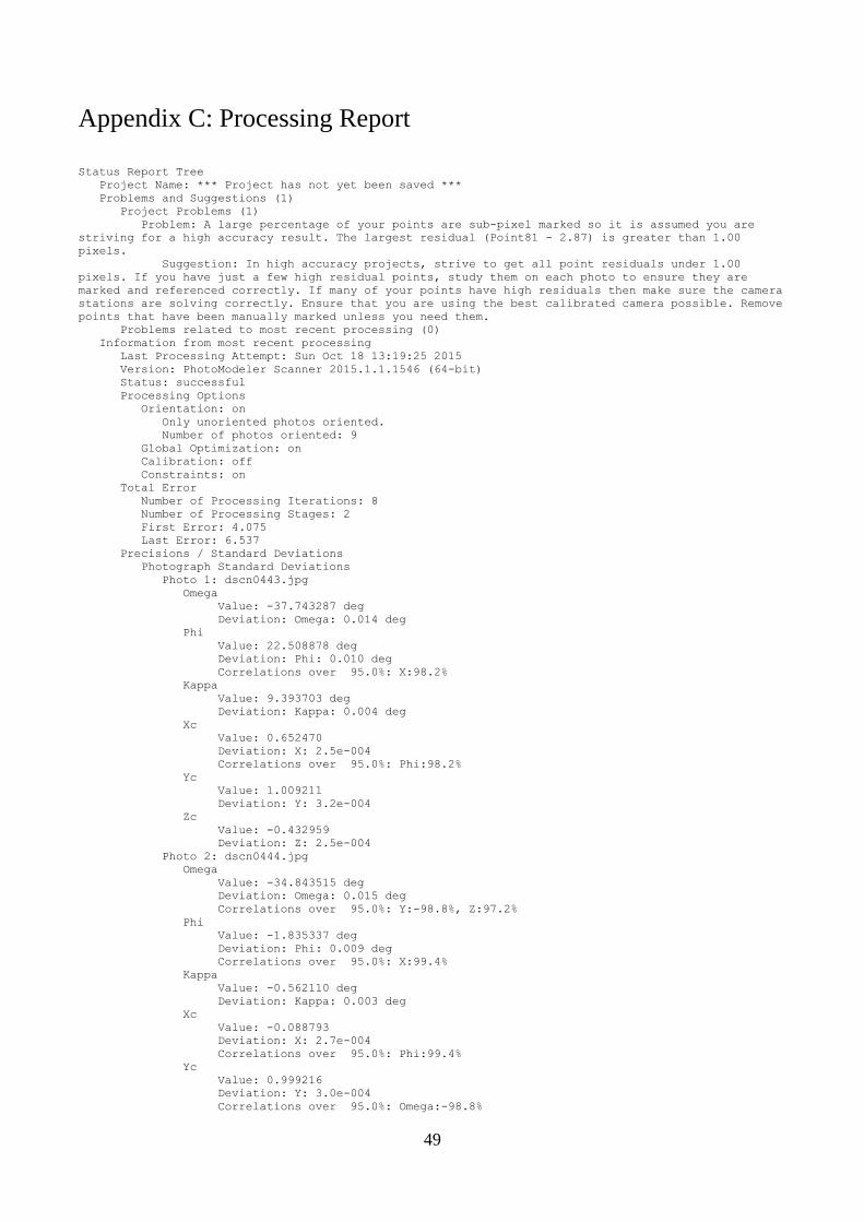
49
Appendix C: Processing Report
Status Report Tree
Project Name: *** Project has not yet been saved ***
Problems and Suggestions (1)
Project Problems (1)
Problem: A large percentage of your points are sub-pixel marked so it is assumed you are
striving for a high accuracy result. The largest residual (Point81 - 2.87) is greater than 1.00
pixels.
Suggestion: In high accuracy projects, strive to get all point residuals under 1.00
pixels. If you have just a few high residual points, study them on each photo to ensure they are
marked and referenced correctly. If many of your points have high residuals then make sure the camera
stations are solving correctly. Ensure that you are using the best calibrated camera possible. Remove
points that have been manually marked unless you need them.
Problems related to most recent processing (0)
Information from most recent processing
Last Processing Attempt: Sun Oct 18 13:19:25 2015
Version: PhotoModeler Scanner 2015.1.1.1546 (64-bit)
Status: successful
Processing Options
Orientation: on
Only unoriented photos oriented.
Number of photos oriented: 9
Global Optimization: on
Calibration: off
Constraints: on
Total Error
Number of Processing Iterations: 8
Number of Processing Stages: 2
First Error: 4.075
Last Error: 6.537
Precisions / Standard Deviations
Photograph Standard Deviations
Photo 1: dscn0443.jpg
Omega
Value: -37.743287 deg
Deviation: Omega: 0.014 deg
Phi
Value: 22.508878 deg
Deviation: Phi: 0.010 deg
Correlations over 95.0%: X:98.2%
Kappa
Value: 9.393703 deg
Deviation: Kappa: 0.004 deg
Xc
Value: 0.652470
Deviation: X: 2.5e-004
Correlations over 95.0%: Phi:98.2%
Yc
Value: 1.009211
Deviation: Y: 3.2e-004
Zc
Value: -0.432959
Deviation: Z: 2.5e-004
Photo 2: dscn0444.jpg
Omega
Value: -34.843515 deg
Deviation: Omega: 0.015 deg
Correlations over 95.0%: Y:-98.8%, Z:97.2%
Phi
Value: -1.835337 deg
Deviation: Phi: 0.009 deg
Correlations over 95.0%: X:99.4%
Kappa
Value: -0.562110 deg
Deviation: Kappa: 0.003 deg
Xc
Value: -0.088793
Deviation: X: 2.7e-004
Correlations over 95.0%: Phi:99.4%
Yc
Value: 0.999216
Deviation: Y: 3.0e-004
Correlations over 95.0%: Omega:-98.8%
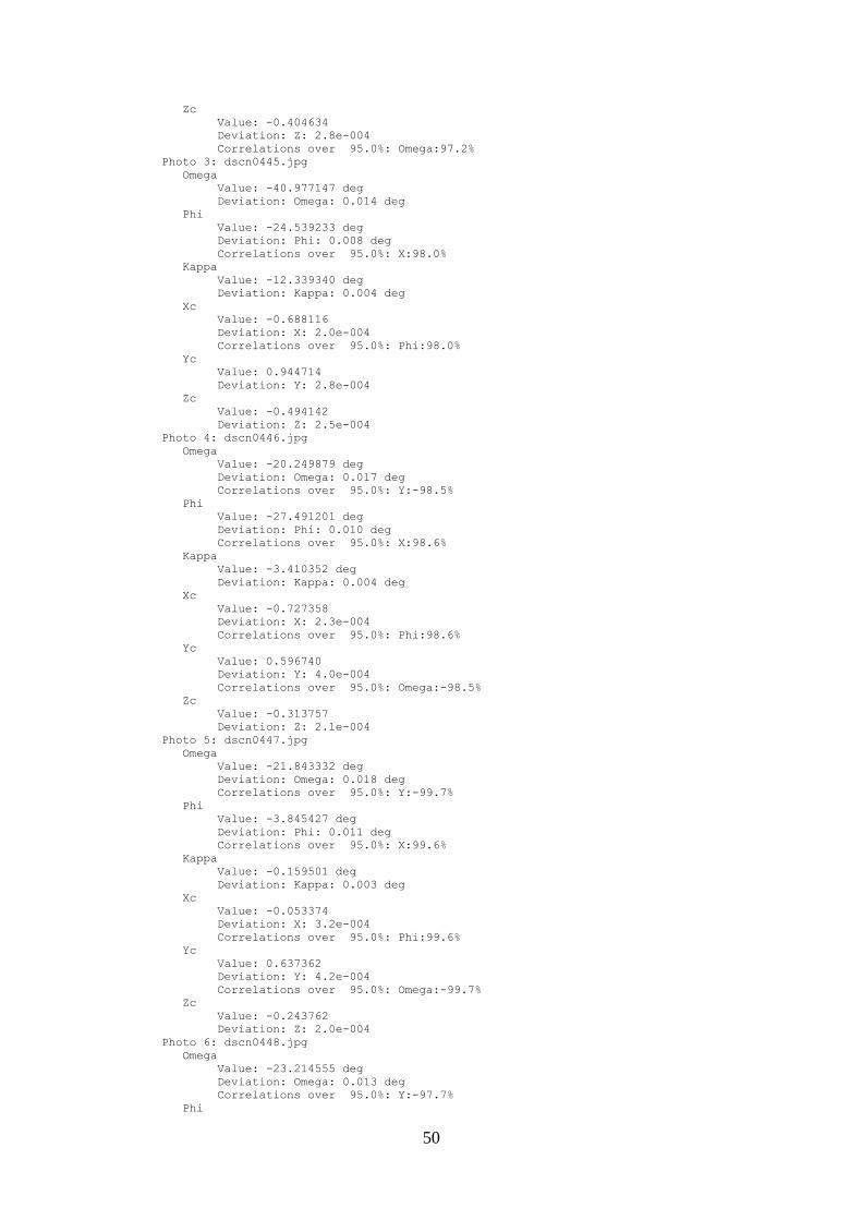
50
Zc
Value: -0.404634
Deviation: Z: 2.8e-004
Correlations over 95.0%: Omega:97.2%
Photo 3: dscn0445.jpg
Omega
Value: -40.977147 deg
Deviation: Omega: 0.014 deg
Phi
Value: -24.539233 deg
Deviation: Phi: 0.008 deg
Correlations over 95.0%: X:98.0%
Kappa
Value: -12.339340 deg
Deviation: Kappa: 0.004 deg
Xc
Value: -0.688116
Deviation: X: 2.0e-004
Correlations over 95.0%: Phi:98.0%
Yc
Value: 0.944714
Deviation: Y: 2.8e-004
Zc
Value: -0.494142
Deviation: Z: 2.5e-004
Photo 4: dscn0446.jpg
Omega
Value: -20.249879 deg
Deviation: Omega: 0.017 deg
Correlations over 95.0%: Y:-98.5%
Phi
Value: -27.491201 deg
Deviation: Phi: 0.010 deg
Correlations over 95.0%: X:98.6%
Kappa
Value: -3.410352 deg
Deviation: Kappa: 0.004 deg
Xc
Value: -0.727358
Deviation: X: 2.3e-004
Correlations over 95.0%: Phi:98.6%
Yc
Value: 0.596740
Deviation: Y: 4.0e-004
Correlations over 95.0%: Omega:-98.5%
Zc
Value: -0.313757
Deviation: Z: 2.1e-004
Photo 5: dscn0447.jpg
Omega
Value: -21.843332 deg
Deviation: Omega: 0.018 deg
Correlations over 95.0%: Y:-99.7%
Phi
Value: -3.845427 deg
Deviation: Phi: 0.011 deg
Correlations over 95.0%: X:99.6%
Kappa
Value: -0.159501 deg
Deviation: Kappa: 0.003 deg
Xc
Value: -0.053374
Deviation: X: 3.2e-004
Correlations over 95.0%: Phi:99.6%
Yc
Value: 0.637362
Deviation: Y: 4.2e-004
Correlations over 95.0%: Omega:-99.7%
Zc
Value: -0.243762
Deviation: Z: 2.0e-004
Photo 6: dscn0448.jpg
Omega
Value: -23.214555 deg
Deviation: Omega: 0.013 deg
Correlations over 95.0%: Y:-97.7%
Phi
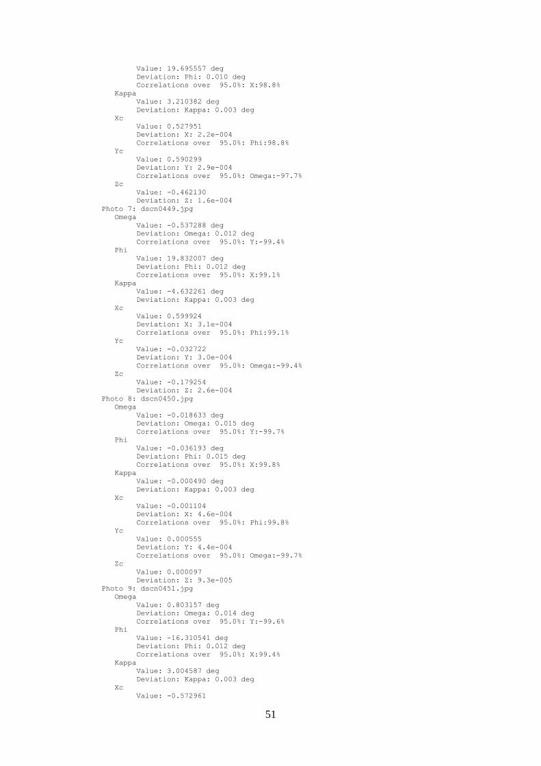
51
Value: 19.695557 deg
Deviation: Phi: 0.010 deg
Correlations over 95.0%: X:98.8%
Kappa
Value: 3.210382 deg
Deviation: Kappa: 0.003 deg
Xc
Value: 0.527951
Deviation: X: 2.2e-004
Correlations over 95.0%: Phi:98.8%
Yc
Value: 0.590299
Deviation: Y: 2.9e-004
Correlations over 95.0%: Omega:-97.7%
Zc
Value: -0.462130
Deviation: Z: 1.6e-004
Photo 7: dscn0449.jpg
Omega
Value: -0.537288 deg
Deviation: Omega: 0.012 deg
Correlations over 95.0%: Y:-99.4%
Phi
Value: 19.832007 deg
Deviation: Phi: 0.012 deg
Correlations over 95.0%: X:99.1%
Kappa
Value: -4.632261 deg
Deviation: Kappa: 0.003 deg
Xc
Value: 0.599924
Deviation: X: 3.1e-004
Correlations over 95.0%: Phi:99.1%
Yc
Value: -0.032722
Deviation: Y: 3.0e-004
Correlations over 95.0%: Omega:-99.4%
Zc
Value: -0.179254
Deviation: Z: 2.6e-004
Photo 8: dscn0450.jpg
Omega
Value: -0.018633 deg
Deviation: Omega: 0.015 deg
Correlations over 95.0%: Y:-99.7%
Phi
Value: -0.036193 deg
Deviation: Phi: 0.015 deg
Correlations over 95.0%: X:99.8%
Kappa
Value: -0.000490 deg
Deviation: Kappa: 0.003 deg
Xc
Value: -0.001104
Deviation: X: 4.6e-004
Correlations over 95.0%: Phi:99.8%
Yc
Value: 0.000555
Deviation: Y: 4.4e-004
Correlations over 95.0%: Omega:-99.7%
Zc
Value: 0.000097
Deviation: Z: 9.3e-005
Photo 9: dscn0451.jpg
Omega
Value: 0.803157 deg
Deviation: Omega: 0.014 deg
Correlations over 95.0%: Y:-99.6%
Phi
Value: -16.310541 deg
Deviation: Phi: 0.012 deg
Correlations over 95.0%: X:99.4%
Kappa
Value: 3.004587 deg
Deviation: Kappa: 0.003 deg
Xc
Value: -0.572961

52
Deviation: X: 3.1e-004
Correlations over 95.0%: Phi:99.4%
Yc
Value: -0.058564
Deviation: Y: 3.6e-004
Correlations over 95.0%: Omega:-99.6%
Zc
Value: -0.135599
Deviation: Z: 2.1e-004
Quality
Photographs
Total Number: 9
Bad Photos: 0
Weak Photos: 0
OK Photos: 9
Number Oriented: 9
Number with inverse camera flags set: 0
Cameras
Camera1: RED S1 COOLPIX S3700 [4.50]
Calibration: yes
Number of photos using camera: 9
Average Photo Point Coverage: 50%
Photo Coverage
Referenced points outside of the camera's calibrated coverage region:
Photo1 points outside region:#24, #48, #23, #22, #47, #21, #20
Photo2 points outside region: more than 10 (check photo and calibration point coverage)
Photo3 points outside region: more than 10 (check photo and calibration point coverage)
Photo4 points outside region: more than 10 (check photo and calibration point coverage)
Photo5 points outside region: more than 10 (check photo and calibration point coverage)
Photo6 points outside region: more than 10 (check photo and calibration point coverage)
Photo7 points outside region: more than 10 (check photo and calibration point coverage)
Photo8 points outside region: more than 10 (check photo and calibration point coverage)
Photo9 points outside region: more than 10 (check photo and calibration point coverage)
Point Marking Residuals
Overall RMS: 0.819 pixels
Maximum: 2.870 pixels
Point 81 on Photo 4
Minimum: 0.454 pixels
Point 55 on Photo 4
Maximum RMS: 1.667 pixels
Point 81
Minimum RMS: 0.324 pixels
Point 68
Point Tightness
Maximum: 0.0017 m
Point 81
Minimum: 0.00026 m
Point 68
Point Precisions
Overall RMS Vector Length: 0.000245 m
Maximum Vector Length: 0.000464 m
Point 84
Minimum Vector Length: 0.000214 m
Point 3
Maximum X: 0.000209 m
Maximum Y: 0.000172 m
Maximum Z: 0.0004 m
Minimum X: 8.81e-005 m
Minimum Y: 7.8e-005 m
Minimum Z: 0.000169 m
Point Angles
Maximum: 64.02 degrees
Point 14
Minimum: 41.2 degrees
Point 80
Average: 58.56 degrees

53
Appendix D: Creating a 3D Dense Surface
The following is a step by step process of how a DSM was created for this project. Tutorial 2, Chapter
5 of the Photomodeler User’s Manual 2013 details these steps to create a DSM of a foot print.
Getting Started
1. Open Photomodeler and start a new project, Automated Targets, for the Getting Started dialog.
2. Follow the New Project Wizard steps.
3. Select RAD – Coded Target Auto-project
4. Select photos of object to be modelled and press Next.
5. Select the camera from the Library you wish to use, e.g. RED S1 COOLPIX S3700 [4.50]
6. A dialog will appear, Automated Coded Target Project, select Run… When the process finishes,
select Close.
Automated Target Marking
7. Go to the Marking menu, select Automatic Target Marking…
8. A dialog will appear, Automatic Target Marking, make sure All Photos is selected from the Photos
from set option, and the correct Target type is selected, e.g. 12-Bit Coded
9. Select Mark Points, wait for the process to finish and then select Close.
10. At this point, Save the project.
Process Project
11. Go to the Project menu and select Process…
12. A dialog will appear, Processing, accept default values and select Process
13. When the processing is complete, select OK. A report can also be saved to a text file to examine
the quality of the project.
14. Go to the Project menu and select Idealise Project. A dialogue will appear stating this step is no
longer necessary. Select either Yes, show me the Idealize dialog or No, exit Idealize. The tutorial
suggestion was adopted to proceed to idealise the photos.
15. After the Idealize step has been completed, follow the prompts to re-process the project.
54
Create DSM
16. For each photo, create a trim around the object, in this case the skull. This can be done by selecting
from the Dense Surface menu – DSM Trim Mode. Draw a line around the skull and double-click on
the start of the line to end.
17. Go to the Dense Surface menu and select Create Dense Surface. In the DSM Options tab, select
Paired photos to use for the DSM. Go through the list and tick the pairs to be used. In the Settings
options, untick Auto depth range and enter an appropriate depth value for the project. In this case,
700mm was more than sufficient to capture the entire skull. Check the correct Units value as well to
avoid errors.
18. Still in the Create Dense Surface window, go to the Meshing Options tab and select Set Defaults.
Then Execute.
Scale Rotate Translate Project
19. Next a scale, coordinate system and rotation can be set for the project. In order to complete this,
there must be a known measurement, such as between two targets, in the project. In the Project menu,
there is an option to use the Scale/Rotate Wizard or Scale/Rotate Viewer. Either can be selected to set
the parameters. For this project, the step by step wizard was initially followed and the Scale/Rotate
Viewer was then used to make any changes necessary. The coordinate system used was simply to set
a particular target as having coordinates, in this case, Point 1 was given X,Y,Z coordinates of 0.0, 0.0,
and 0.0.
3D Model DSM
19. Open the 3D View Window in the Tools Bar. There are a number of different surfaces that can be
displayed and also measurements can be take using the Measurements tool between points and lines.
The model can be exported to other file formats if required. There are many useful tools and display
options available in the 3D View Window.