The use of linear programming in the analysis of petrological mixing problems

Contrib. Mineral. Petrol. 70, 237-244 (1979) Contributions to Mineralogy and Petrology �9 by Springer-Verlag 1979

The Use of Linear Programming in the Analysis of Petrological Mixing Problems

Roger Banks

Department of Environmental Sciences, University of Lancaster, Lancaster, England

Abstract. Petrological mixing problems such as modal analysis, magma mixing, and liquid line of descent calculations, can be solved using the methods of linear programming. If estimates of the standard error of the chemical data are introduced as weights into the set of equations, it is possible to assign confidence limits to the solutions which are obtained and to apply formal statistical tests to geological hypotheses based on the mixing model. This approach is applied to petrological data previously analysed by Wright and Doherty (1970) using a combination of linear programming and least squares methods. It is shown that some of the geological inferences which they drew were based on an overoptimistic assessment of the confidence limits on their solutions, and cannot be regarded as proven.

1. Introduction

The analysis of a petrological mixing problem involves the solution of an overdetermined set of linear equations. For example, an attempt may be made to represent the bulk chemical composition of a rock in terms of the relative proportions of a number of mineral phases. The chemical compositions of both the rock and the supposed constituent minerals are known from experimental measurements. The composition of the rock is assumed to be related to that of the mineral phases by the equation

L

Tj= ~ Vj~y~ j=I,M. (1)

In this expression, Vjl is the weight percentage of the j th oxide in the lth mineral phase, Yt is the fraction of the lth phase present in the mode, and Tj is the weight percentage of the jth oxide in the rock. (In this

paper, the term 'mode ' is generally used to mean the mineralogical composition of a rock derived from a chemical analysis, rather than from the more usual microscopic investigation, and the term 'chemical mode' might be more correct). M is the number of oxides which have been analysed, and the rock is considered to be made up from no more than the L mineral phases included in the mode, so it is implicit that

L

E y, = 1. (21 l - 1

The aim of a modal analysis is to attempt to match the composition of the synthetic rock, Tj(j = I , M ) , to the composition of an actual rock, of which the chemical composition, Xj(j=I,M), has been determined in the laboratory. The success of the mode can be judged by examining the misfits

Xj - Tj = dj (31

between the observed and predicted oxide weight percentages. Thus the mathematical problem to be solved in a modal analysis is that of finding a solution y~(I=l,L) of Eq.(1) which minimises some measure of the misfit.

A measure which is frequently used is the sum of the squares of the individual misfits; and it is a relatively straightforward matter to find the solution which minimises this misfit. However, solutions of such unconstrained least squares problems suffer from the disadvantage that they may be either positive or negative. In the context of a modal analysis, a negative proportion has no physical reality. It would be preferable, in fact, to constrain the solution in such a way that all the resulting components were forced to be positive.

Wright and Doherty (1970) suggested that this difficulty could be overcome by employing a two-

0010-7999/79/0070/0237/$01.60

238 R. Banks: Linear Programming Solutions to Petrological Mixing Problems

stage method. They pointed out that it is possible to solve a constrained linear problem using the techniques of linear programming, provided that a linear measure of the overall misfit is used, rather than the normal quadratic measure. In most cases, the solution obtained by linear programming is found to involve zero values for a number of the mineral phases. These are the phases which would possibly yield negative values in the least squares analysis, and are consequently rejected. The remaining components define a new mode, the proportions of which are determined by a least squares calculation.

Wright and Doherty (1970) do not make clear their reasons for proceeding beyond the initial linear programming stage. They state that they used the single-stage linear programming approach in one case, and obtained results which differed significantly from those achieved by the least squares method. My own experience has been that the results which are obtained using linear programming alone, and a linear measure of misfit, are directly comparable to those achieved by Wright and Doherty (1970) using the two stage approach, and a quadratic measure of misfit. In addition, it is possible to set up formal statistical tests to assist in assessing the 'goodness of fit' of the mode; something which Wright and Doh- erty (1970) did not seriously attempt.

2. Measures of Misfit and Their Statistical Assessment

The most commonly used measure of the misfit between a set of observations and a corresponding set of values predicted by a theory or model, is the sum of the squares of the individual misfits (the L 2 norm):

j--i

If the individual misfits are normalised by the standard errors aj of the corresponding observations, the result is the chi-squared statistic:

j = l \ O-j I "

A formal statistical test of the acceptability of a particular misfit, Z 2, can be set up in the following way. The null hypothesis is that the observations Xj are a sample from a population which is correctly described by the mode Tj. The individual misfits are normally distributed with zero mean and standard deviation c 0. The probability, P, that the value of X 2, with M degrees of freedom, exceeds )f~, can be found by consulting suitable statistical tables. For instance, if there are 10 data and X2=18.31, then P=0.05. In other words, with a misfit this large, there is only a 1 in 20 chance that the null hypothesis is correct, and we say that it can be rejected at the 95 % [ = 100(1-P)] confidence level.

The disadvantage of the 22 statistic is that it is a quadratic function of the individual misfits, and cannot be incorporated within the framework of linear programming. Quadratic pro-

gramming is possible, but is much more expensive in terms of computer time. The alternative is to find a measure of the overall misfit between observation and model which is a linear combination of the individual misfits. A measure meeting this requirement is the sum of the absolute values of the individual misfits (the L 1 norm):

~=~ xj- r~. (4)

j= 1 tTj

Tables of the probability P that y exceeds a specified value have been computed for up to 10 data (Hartley and Godwin, 1945), but standard tables rarely contain this information. However, when M is sufficiently large, the distribution function of 7 becomes approxi- mately normal, with mean

= (2 M ( M - 1)fiz) }

and standard deviation

An approximation which is adequate for most purposes when M_>_ 10 is

~- M (2fij ~,

s-~ [M(1 - 2/~z)]<

The probability that the misfit between the observations and the modal composition exceeds y., is

P{Y>Ym; M data}-~P{Y> Y,.}

1 r~ : 1 - ~ ~ e - r 2 n d Y (5 /

Vz~ - c o

where Y - ( y - 7 ) I s is the normally distributed variable with mean and standard deviation s appropriate to the number of data, M.

Tabulated values of the normal probability integral in the form required by Eq. (5) are commonly available in statistical tables. A comparison of the exact probability given by Hartley and Godwin (1945) with the value obtained by using the normal approximation shows that the latter is valid for most purposes when the number of data is 10 or more.

3. Modal Analysis as a Linear Programming Problem

Consider, as an illustration, the problem of achieving the optimum representation of the chemical composition of a rock, in terms of a number of mineral phases. The example given by Wright and Doherty (1970) in Table 1A, a modal analysis of a prehistoric basalt from Makaopuhi lava lake, Hawaii, provides the data.

The first requirement in setting up the linear programming equations, must be that the abundance of each oxide in the theoretical mode, Tj, fits the measured abundance in the rock, Xj, to within a certain error, d r [Eq. (3)]. The theoretical composition can be expressed in terms of the compositions of the mineral phases, Vjl, and the fractions Yz of each which are present [Eq. (1)]. In order to assign equal weight to each of the data, the equations are

R. Banks: Linear Programming Solutions to Petrological Mixing Problems

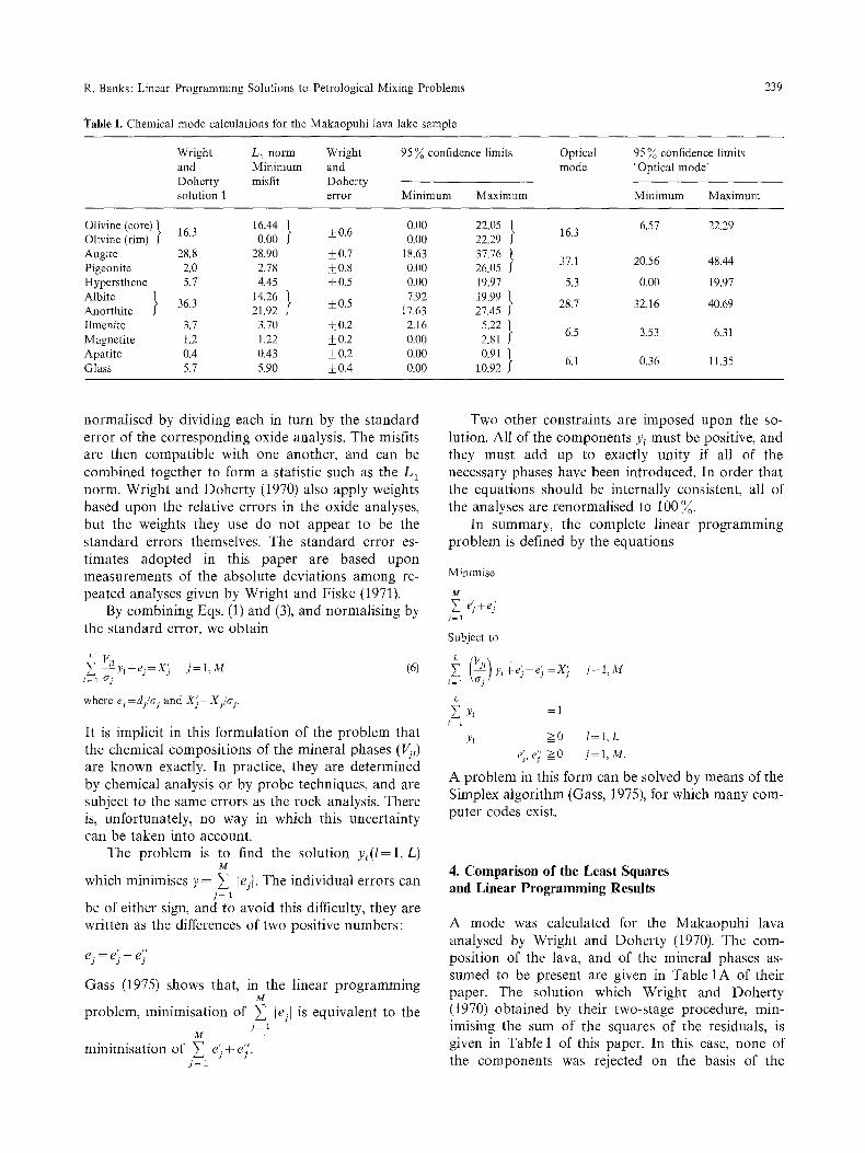
Table 1. Chemical mode calculations for the Makaopuhi lava lake sample

239

Wright L~ norm Wright 95 ~o confidence limits and Minimum and Doherty misfit Doherty solution l error Minimum Maximum

Optical 95 % confidence limits mode ' Optical mode'

Minimum Maximum

Olivine(core)} 16.44 } +0.6 0.00 22.05 Olivine (rim) 16.3 0.00 - 0.00 22.29 Augite 28.8 28.90 • 0.7 18.63 37.76 Pigeonite 2.0 2.78 + 0.8 0.00 26.05 Hypersthene 5.7 4.45 +0.5 0.00 19.97 albite } 3 6 . 3 14.26} +0.5 7.92 19.99 Anorthite 21.92 - 17.63 27.45 Ilmenite 3.7 3.70 • 0.2 2.16 5.22 Magnetite 1.2 1.22 • 0.2 0.00 2.81 Apatite 0.4 0.43 • 0.2 0.00 0.91 Glass 5.7 5.90 _+ 0.4 0.00 10.92

16.3 6.57 22.29

37.1 20.56 48.44

5.3 0.00 19.97

28.7 32.16 40.69

6.5 3.53 6.3i

6.1 0.36 11.35

normalised by dividing each in turn by the standard error of the corresponding oxide analysis. The misfits are then compatible with one another, and can be combined together to form a statistic such as the L 1 norm. Wright and Doherty (1970) also apply weights based upon the relative errors in the oxide analyses, but the weights they use do not appear to be the standard errors themselves. The standard error estimates adopted in this paper are based upon measurements of the absolute deviations among re- peated analyses given by Wright and Fiske (1971).

By combining Eqs. (1) and (3), and normal• by the standard error, we obtain

Vj~yl§ ~ j=I,M (6) l = l O'j

where ej=d/% and Xj =X/%.

It is implicit in this formulation of the problem that the chemical compositions of the mineral phases (Vj~) are known exactly. In practice, they are determined by chemical analysis or by probe techniques, and are subject to the same errors as the rock analysis. There is, unfortunately, no way in which this uncertainty can be taken into account.

The problem is to find the solution yz(l=l, L) M

which minimises ? = ~ ]%1. The individual errors can j - 1

be of either sign, and to avoid this difficulty, they are written as the differences of two positive numbers:

%=e)-e) '

Gass (1975) shows that, in the linear programming i

problem, minim•177 of ~ [ejI is equivalent to the j - - 1

M

minim•177 of ~ e}+e}'. j = l

Two other constraints are imposed upon the solution. All of the components Yz must be positive, and they must add up to exactly unity if all of the necessary phases have been introduced. In order that the equations should be internally consistent, all of the analyses are renormalised to 100 ~o.

In summary, the complete linear programming problem is defined by the equations

Minimise

M Ct r~

j + e j j = l

Subject to

l=l Y l §

~ y~ =1 I=I

Yl >0 I=I,L e~,e)' >0 j=I,M.

A problem in this form can be solved by means of the Simplex algorithm (Gass, 1975), for which many computer codes exist.

4. Comparison of the Least Squares and Linear Programming Results

A mode was calculated for the Makaopuhi lava analysed by Wright and Doherty (1970). The composition of the lava, and of the mineral phases assumed to be present are given in Table 1A of their paper. The solution which Wright and Doherty (1970) obtained by their two-stage procedure, minim• the sum of the squares of the residuals, is given in Table 1 of this paper. In this case, none of the components was rejected on the basis of the


linear programming analysis. Consequently, the solution can be directly compared with my linear programming solution based on the minimisation of the L1 norm, which is given in column 2 of Table 1. The agreement is extremely good; the only significant discrepancies are for pigeonite and hypersthene, and they are relatively small. It is clear that, in this case at least, the minimisation of the sum of squares and the minimisation of the sum of absolute values of misfits lead to the same optimum solution.

The value of the misfit for my best-fitting solution is 7,~ = 0.624. This represents an extremely good fit to the data. The expected value of 7 for 11 data is (see Sect. 2) ]=8.78. Its standard deviation s=2.00. Thus the probability that Y should be greater than 0.624 is [Eq. (5)] 0.99998. In other words, there is only 1 chance in 50,000 of obtaining a fit as good as this. Given the quality of the data it is wrong to demand that the fit of a model to the data should be so good. There must be many other solutions (in fact an infinite number) which fit these data at an acceptable confidence level, and no special importance should be attached to the solution which happens to fit it best.

However, it is still necessary to find some means of characterising the class of acceptable solutions, and of defining limits on the proportions of each modal constituent. Wright and Doherty's approach to this problem is to allow each of the mineral proportions to vary independently, starting from the minimum misfit solution. Each proportion is varied until the resulting misfit becomes unacceptable, judged on the basis of the size of the largest individual misfit and the average of the absolute values of the misfits. The changes in the mineral proportions which Wright and Doherty (1970) determined as giving rise to unacceptable misfits are listed in the third column of Table 1.

There are two objections to this procedure, as Wright and Doherty (1970) themselves admit. First, the individual components are varied separately, rather than together. If all components were allowed to vary simultaneously, an increase in the amount of olivine in the mode, for instance, might be com- pensated by a corresponding decrease in the amount Of augite. Instead, olivine is varied while augite is held constant, and such compensation is not allowed. The consequence is that error estimates based upon the independent variation of solution parameters grossly underestimate the real uncertainty of the solutions. The second objection is that the scan of solutions always starts with the minimum misfit model. As a result, only that part of the solution space immediately adjacent to the minimum misfit mode is investigated. It is conceivable that other solutions exist which fit the data adequately, but which are too

'far' from the minimum misfit mode to be reached by Wright and Doherty's procedure.

These difficulties can be avoided by using linear programming to investigate the characteristics of all solutions which satisfy the data at a chosen confidence level. This is most easily achieved by defining a level of misfit which separates unacceptable solutions from the rest. In this investigation, the 5 ~o confidence level has been used as the dividing line. The level of misfit, y', corresponding to this bound- ary, is defined by the condition

P{7>7' ; 11 data}=0.05.

There is only a 1 in 20 chance of a misfit larger than ~' occurring, if the theoretical mode truly represents the observed composition. Accordingly, we say that modes with misfits larger than y' can be rejected at the 95 ~o confidence level.

From Eq. (5), it follows that 7' is defined by the expression

1 I" 0.95-- - ] /~ 5co e-r=/2dY

where Y'=(~'-~)/s. From tables of the normal distribution function, we find that this equation is satisfied by Y'=1.645, corresponding to a misfit 7'=12.065. Thus, solutions which have a misfit of 12.065 or more can be rejected at the 95~o confidence level. Con- versely, 'acceptable' solutions are those for which

< 12.065. The original objective of the linear programming

problem defined in Sect. 3 was the minimisation of the L 1 norm. The aim now is to find the characteristics of those solutions which satisfy the additional constraint

M Z e) + ey< 12.065.

j = l

The bounds on acceptable solutions are investigated by minimising or maximising different components of the solution in turn. For instance, if l= 3 corresponds to the composition of augite, the solution to the linear programming problem which minimises Y3 will be the modal composition which contains the small- est possible amount of augite and still just satisfies the data with a misfit of 12.065. The lower and upper limits on the proportions of each mineral phase were obtained in this way, and are displayed in columns 4 and 5 of Table 1. Comparison with Wright and DohertY'S error estimates reveals the extent to which their approach underestimates the range of modal compositions which is compatible with the data.

R. Banks: Linear Programming SoIutions to Petrological Mixing Problems

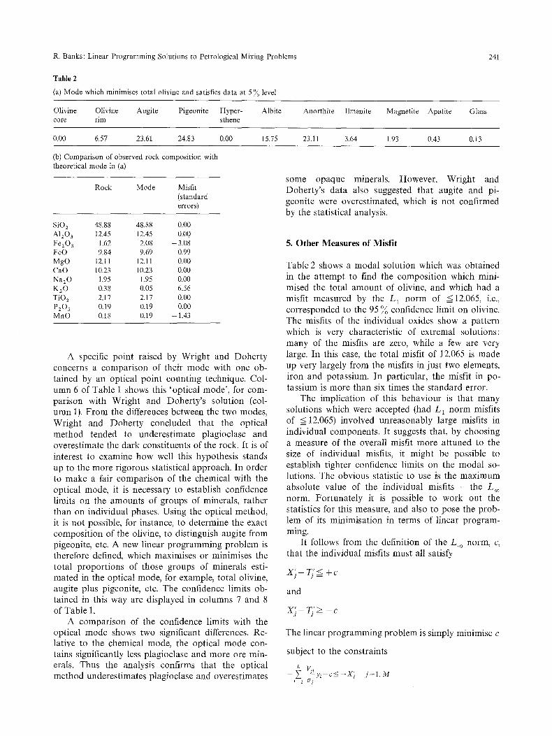
Table 2

(a) Mode which minimises total olivine and satisfies data at 5 ~o level

241

Olivine Olivine Augite Pigeonite Hyper- Albite Anorthite Ilmenite Magnetite Apatite Glass core rim sthene

0.00 6.57 23.61 24.83 0.00 15.75 23.11 3.64 1.93 0.43 0.13

(b) Compar ison of observed rock composit ion with theoretical mode in (a)

Rock Mode some opaque minerals. However, Wright and

Misfit Doherty's data also suggested that augite and pi- (standard errors) geonite were overestimated, which is not confirmed

by the statistical analysis. SiO 2 48.88 48.88 0.00 A120 3 12.45 12.45 0.00 Fe20 3 1.62 2.08 - 3,08 FeO 9.84 9.69 0.99 MgO 12.11 12.11 0.00 CaO 10,23 10.23 0.00 Na~O 1,95 1.95 0.00 K 2 0 0.38 0.05 6.56 TiO 2 2.17 2.17 0.00 P2Os 0.19 0.19 0.00 M n O 0.18 0.19 - 1.43

A specific point raised by Wright and Doherty concerns a comparison of their mode with one obtained by an optical point counting technique. Col- umn 6 of Table 1 shows this 'optical mode', for comparison with Wright and Doherty's solution (column 1). From the differences between the two modes, Wright and Doherty concluded that the optical method tended to underestimate plagioclase and overestimate the dark constituents of the rock. It is of interest to examine how well this hypothesis stands up to the more rigorous statistical approach. In order to make a fair comparison of the chemical with the optical mode, it is necessary to establish confidence limits on the amounts of groups of minerals, rather than on individual phases. Using the optical method, it is not possible, for instance, to determine the exact composition of the olivine, to distinguish augite from pigeonite, etc. A new linear programming problem is therefore defined, which maximises or minimises the total proportions of those groups of minerals esti- mated in the optical mode, for example, total olivine, augite plus pigeonite, etc. The confidence limits obtained in this way are displayed in columns 7 and 8 of Table 1.

A comparison of the confidence limits with the optical mode shows two significant differences. Re- lative to the chemical mode, the optical mode contains significantly less plagioclase and more ore minerals. Thus the analysis confirms that the optical method underestimates plagioclase and overestimates

5. Other Measures of Misfit

Table 2 shows a modal solution which was obtained in the attempt to find the composition which mini- raised the total amount of olivine, and which had a misfit measured by the L 1 norm of <12.065, i.e., corresponded to the 95 ~o confidence limit on olivine. The misfits of the individual oxides show a pattern which is very characteristic of extremal solutions: many of the misfits are zero, while a few are very large. In this case, the total misfit of 12.065 is made up very largely from the misfits in just two elements, iron and potassium. In particular, the misfit in potassium is more than six times the standard error.

The implication of this behaviour is that many solutions which were accepted (had L 1 norm misfits of <12.065) involved unreasonably large misfits in individual components. It suggests that, by choosing a measure of the overall misfit more attuned to the size of individual misfits, it might be possible to establish tighter confidence limits on the modal solutions. The obvious statistic to use is the maximum absolute value of the individual misfits - the L~ norm. Fortunately it is possible to work out the statistics for this measure, and also to pose the problem of its minimisation in terms of linear programming.

It follows from the definition of the Loo norm, c, that the individual misfits must all satisfy

Xj - r j ' ~ + c

and

X j . - r j t ~ - c

The linear programming problem is simply minimise c

subject to the constraints

- ~ vJ'y,-c__<-x) j=I ,M l-1 0j


Vjzy~-c<=Xj j = I , M I = l O'j

Yz >0 l = l , L

~Yl =1 / = 1

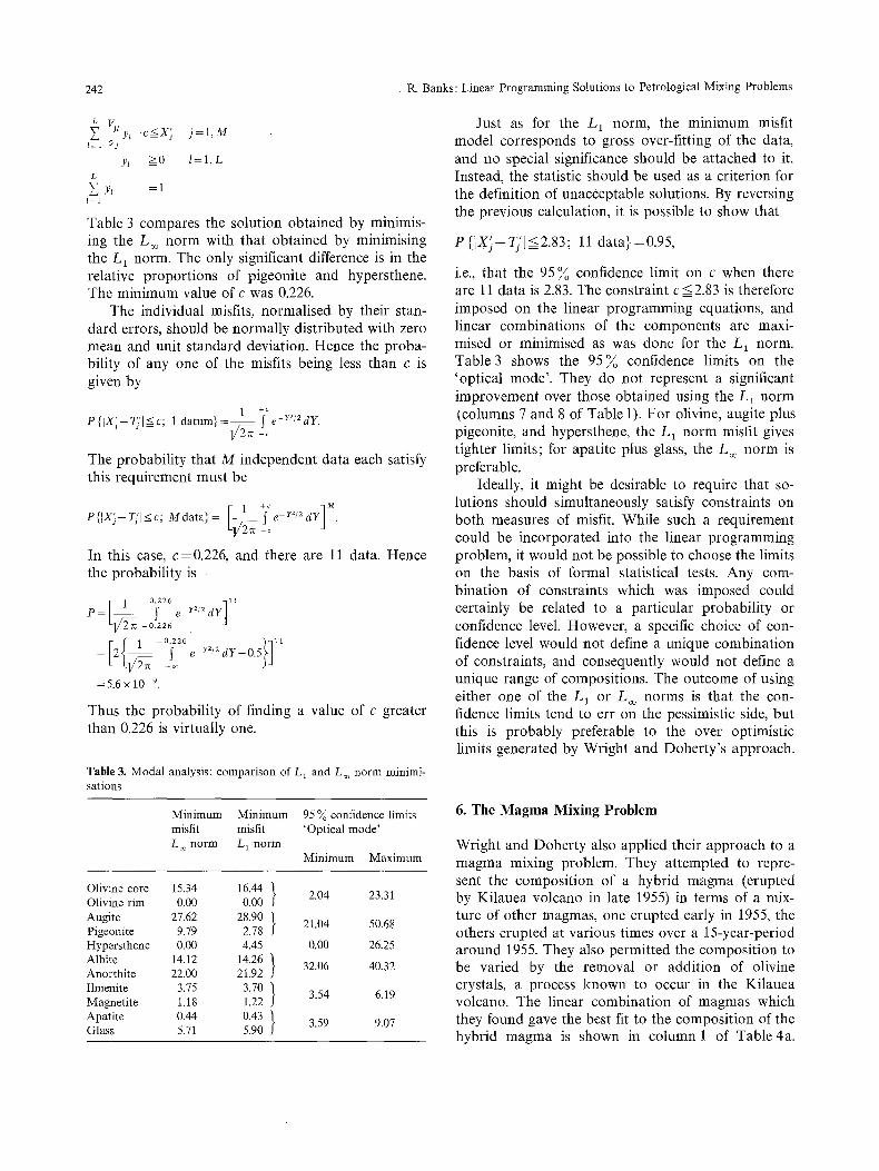
Table 3 compares the solution obtained by minimising the L~ norm with that obtained by minimising the Lt norm. The only significant difference is in the relative proportions of pigeonite and hypersthene. The minimum value of c was 0.226.

The individual misfits, normalised by their standard errors, should be normally distributed with zero mean and unit standard deviation. Hence the probability of any one of the misfits being less than c is given by

1 +c P { l X ~ - T j l < c ; 1 d a t u m } = ~ y e-r~/2dy.

Vz~ - c

The probability that M independent data each satisfy this requirement must be

r 1 +c 3M P{lXS- rjl<c; Mdata}= / - - ~ e-r2/Z d Y | .

I - l ~ c 1

In this case, c=0.226, and there are 11 data. Hence the probability is

P = [. e- r2/2 dY 0.226

E2{ }1 = S e - r2 /2dY-0"5 - c o

=5.6 x 10 9.

Thus the probability of finding a value of c greater than 0.226 is virtually one.

Table 3. Modal analysis: comparison of L 1 and L~ norm minimi- sations

Minimum Minimum 95 % confidence limits misfit misfit 'Optical mode' Loo norm g 1 norm

Minimum Maximum

Olivine core 15.34 16.44 } 2.04 23.31 Olivine rim 0.00 0.00 Augite 27.62 28.90 } 21.04 50.68 Pigeonite 9.79 2.78 Hypersthene 0.00 4.45 0.00 26.25 Albite 14.12 14.26 } Anorthite 22.00 21.92 32.06 40.32

Ilmenite 3.75 3.70 } 3.54 6.19 Magnetite 1.18 1.22 Apatite 0.44 0.43 } Glass 5.71 5.90 3.59 9.07

Just as for the L1 norm, the minimum misfit model corresponds to gross over-fitting of the data, and no special significance should be attached to it. Instead, the statistic should be used as a criterion for the definition of unacceptable solutions. By reversing the previous calculation, it is possible to show that

P {IXj- Tj'[ <2.83; 11 data} =0.95,

i.e., that the 95 % confidence limit on c when there are 11 data is 2.83. The constraint c<2.83 is therefore imposed on the linear programming equations, and linear combinations of the components are maxi- raised or minimised as was done for the L 1 norm. Table 3 shows the 95% confidence limits on the 'optical mode'. They do not represent a significant improvement over those obtained using the L1 norm (columns 7 and 8 of Table 1). For olivine, augite plus pigeonite, and hypersthene, the L 1 norm misfit gives tighter limits; for apatite plus glass, the Loo norm is preferable.

Ideally, it might be desirable to require that solutions should simultaneously satisfy constraints on both measures of misfit. While such a requirement could be incorporated into the linear programming problem, it would not be possible to choose the limits on the basis of formal statistical tests. Any combination of constraints which was imposed could certainly be related to a particular probability or confidence level. However, a specific choice of confidence level would not define a unique combination of constraints, and consequently would not define a unique range of compositions. The outcome of using either one of the L 1 or Loo norms is that the confidence limits tend to err on the pessimistic side, but this is probably preferable to the over optimistic limits generated by Wright and Doherty's approach.

6. The Magma Mixing Problem

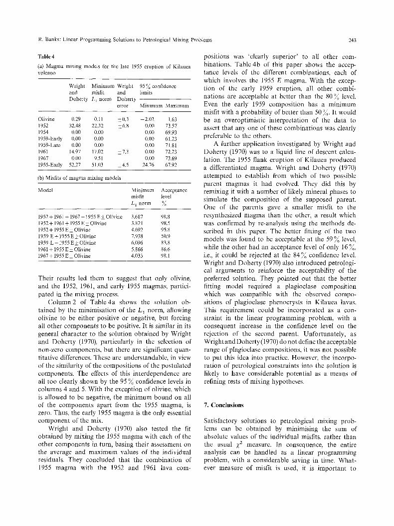
Wright and Doherty also applied their approach to a magma mixing problem. They attempted to represent the composition of a hybrid magma (erupted by Kilauea volcano in late 1955) in terms of a mix- ture of other magmas, one erupted early in 1955, the others erupted at various times over a 15-year-period around 1955. They also permitted the composition to be varied by the removal or addition of olivine crystals, a process known to occur in the Kilauea volcano. The linear combination of magmas which they found gave the best fit to the composition of the hybrid magma is shown in column 1 of Table 4a.

R. Banks: Linear Programming Solutions to Petrological Mixing Problems 243

Table 4

(a) Magma mixing models for the late 1955 eruption of Kilauea volcano

Wright Minimum Wright 95 % confidence and misfit and limits Doherty L 1 norm Doherty

error Minimum Maximum

Olivine 0.29 0.11 +0.3 -2.02 1.63 1952 32.48 22.32 +6.8 0.00 73.57 1954 0.00 0.00 0.00 69.93 1959-Early 0.00 0.00 0.00 61.23 1959-Late 0.00 0.00 0.00 71.81 1961 14.97 17.02 _+ 7.3 0.00 72.23 1967 0.00 9.51 0.00 73.69 1955-Early 52.27 51.03 +4.5 24.76 67.92

(b) Misfits of magma mixing models

Model Minimum Acceptance misfit level L 1 norm %

1952 + 1961+ 1967 + 1955 E_+ Olivine 3.687 98.8 1952 + 1961 + 1955 E • Olivine 3.821 98.5 1952 + 1955 E • Olivine 4.692 95.8 1959-E + 1955 E • Olivine 7.938 50.9 1959-L + 1955 E + Olivine 6.096 83.8 1961 + 1955 E-t- Olivine 5.866 86.6 1967 + 1955 E _+ Olivine 4.033 98.1

Their results led them to suggest that only olivine, and the 1952, 1961, and early 1955 magmas, partici- pated in the mixing process.

Co lumn2 of Table 4a shows the solution obtained by the minimisation of the L 1 norm, allowing olivine to be either positive or negative, but forcing all other components to be positive. It is similar in its general character to the solution obtained by Wright and Doherty (1970), particularly in the selection of non-zero components, but there are significant quan- titative differences. These are understandable, in view of the similarity of the compositions of the postulated components. The effects of this interdependence are all too clearly shown by the 95 % confidence levels in columns 4 and 5. With the exception of olivine, which is allowed to be negative, the minimum bound on all of the components apart from the 1955 magma, is zero. Thus, the early 1955 magma is the only essential component of the mix.

Wright and Doherty (1970) also tested the fit obtained by mixing the 1955 magma with each of the other components in turn, basing their assessment on the average and maximum values of the individual residuals. They concluded that the combination of 1955 magma with the 1952 and 1961 lava corn-

positions was 'clearly superior ' to all other combinations. Table 4b of this paper shows the acceptance levels of the different combinations, each of which involves the 1955 E magma. With the exception of the early 1959 eruption, all other combinations are acceptable at better than the 80% level. Even the early 1959 composition has a minimum misfit with a probability of better than 50 ~0. It would be an overoptimistic interpretation of the data to assert that any one of these combinations was clearly preferable to the others.

A further application investigated by Wright and Doherty (1970) was to a liquid line of descent calculation. The 1955 flank eruption of Kilauea produced a differentiated magma. Wright and Doherty (1970) at tempted to establish from which of two possible parent magmas it had evolved. They did this by remixing it with a number of likely mineral phases to simulate the composition of the supposed parent. One of the parents gave a smaller misfit to the resynthesized magma than the other, a result which was confirmed by re-analysis using the methods described in this paper. The better fitting of the two models was found to be acceptable at the 59 % level, while the other had an acceptance level of only 16 %, i.e., it could be rejected at the 84 % confidence level. Wright and Doherty (1'970) also introduced petrological arguments to reinforce the acceptability of the preferred solution. They pointed out that the better fitting model required a plagioclase composition which was compatible with the observed compositions of plagioclase phenocrysts in Kilauea lavas. This requirement could be incorporated as a constraint in the linear programming problem, with a consequent increase in the confidence level on the rejection of the second parent. Unfortunately, as Wright and Doherty (1970) do not define the acceptable range of plagioclase compositions, it was not possible to put this idea into practice. However, the incorpo- ration of petrological constraints into the solution is likely to have considerable potential as a means of refining tests of mixing hypotheses.

7. Conclusions

Satisfactory solutions to petrological mixing problems can be obtained by minimising the sum of absolute values of the individual misfits, rather than the usual ;~2 measure. In consequence, the entire analysis can be handled as a linear programming problem, with a considerable saving in time. What- ever measure of misfit is used, it is important to


incorporate into the analysis estimates of the errors in the chemical data. If the equations are weighted by the standard errors in the data, proper statistical confidence limits can be assigned to the solutions.

The results obtained by the application of this technique to modal analysis and other petrological mixing problems, suggest that in some cases the geochemical data are not sufficiently precise to discrim- inate among the hypotheses being tested. To strength- en the conclusions, it will be necessary to incorporate more data (minor or trace element analyses), to reduce the errors in the data, or to impose petrological constraints upon the solutions. The last approach offers the most possibilities, and can in many cases be achieved within the framework of linear programming.

References

Gass, S.I.: Linear programming: methods and applications. NewYork: McGraw-Hill 1975

Hartley, H.O., Godwin, H.J.: Tables of the probability integral of the mean deviation in normal samples. Biometrika 33, 259-265 (1945)

Wright, T.L., Doherty, P.C.: A linear programming and least squares computer method for solving petrologic mixing problems. Bull. Geol. Soc. Am. 81, 1995-2008 (1970)

Wright, T.L., Fiske, R.S.: Origin of the differentiated and hybrid lavas of Kilauea volcano, Hawaii. J. Petrol. 12, 1-65 (1971)

Received April 17, 1979; Accepted July 2, 1979

Documents

The use of linear programming in the analysis of petrological mixing problems