Embed Size (px)
Citation preview
The use of historical datasets to develop multi-trait selectionmodels in processing tomato
Debora Liabeuf . David M. Francis
Received: 7 November 2016 / Accepted: 9 March 2017 / Published online: 6 April 2017
� The Author(s) 2017. This article is an open access publication
Abstract Multi-trait indices (MTI) weigh traits
based on their importance to facilitate selection in
plant and animal improvement. In animal breeding,
economic values are used to develop MTIs. For
vegetables, economic data valuing traits are rarely
available. We posit that varieties with traits valued by
growers and processors achieve higher market share
and longer life span. Our objective was to develop
MTIs predicting success of tomato varieties. Histor-
ical data for the California processing tomato industry
from 1992 to 2013 provided measurements for yield,
soluble solids (Brix), color, pH, market share, and life
span for 258 varieties. We used random models to
estimate best linear unbiased predictors (BLUPs) for
phenotypic traits of each variety, and evaluated trends
over time. Yield has been increasing from 2006, while
Brix stayed constant. Because yield and Brix are
negatively correlated, this trend suggests that Brix
influenced selection. The average number of resis-
tances reported in varieties ranking in the top ten
increased from 2 to 4.5 between 1992 and 2013. MTIs
predicting success from phenotypic traits were
developed with general linear models and tested using
leave-one-out cross validation. MTIs weighing yield,
Brix, pH and color were significantly correlated to
success metrics and selected a significantly higher
proportion of successful varieties relative to random
sampling. The index multiplying yield and brix,
suggested in the literature, was not significantly
correlated with variety success. The MTIs suggested
that fruit quality had less of an influence on variety
success than yield. The MTIs developed could help
improve gain under selection for quality traits in
addition to yield.
Keywords Solanum lycopersicum � Multi-trait
index � Breeding � Market share � Market life-span �General linear model
Introduction
The recent interest in selectionmodels that incorporate
marker data and kinship to estimate breeding values
(Meuwissen et al. 2001) is reviving interest in
approaches that allow data for phenotypic traits to be
combined and balanced. Multi-trait indices (MTIs) are
an approach to select for more than one characteristic.
MTIs are expected to be particularly valuable for crops
where quality traits are of importance for market
success. MTIs based on economic values have been
widely used and described in the animal breeding
Electronic supplementary material The online version ofthis article (doi:10.1007/s10681-017-1876-6) contains supple-mentary material, which is available to authorized users.
D. Liabeuf � D. M. Francis (&)
Ohio Agricultural Research and Development Center, The
Ohio State University, 1680 Madison Ave, Wooster,
OH 44691, USA
e-mail: [email protected]
123
Euphytica (2017) 213:100
DOI 10.1007/s10681-017-1876-6
literature (Cottle and Coffey 2013; De Haas et al.
2013; Laske et al. 2012; Visscher et al. 1994). For
plants this approach is advocated (Eathington et al.
2007; Merk et al. 2012), but such MTIs are generally
not described in the literature. One exception are the
models based on net merit that were explored for
wheat in order to integrate grain yield, plant charac-
teristics and milling quality with economic weights
(Heffner et al. 2011). Trait valuation in the market is
lacking for many characteristics considered important
for vegetable crops. In the absence of economic data
for trait value, an alternative approach may be to
developMTIs based on the historical characteristics of
varieties that are proven to be successful in the market.
The performance of processing tomato varieties
needs to conform to growers’ and processors’ expec-
tations, the United States Department of Agriculture
grade standards (U.S. Department of Agriculture
1990), and consumer preferences. Growers prefer high
yield, uniform ripening, long field storage of fruit,
resistance to a variety of root and foliar pathogens, and
a plant habit suitable for mechanical harvest (Stevens
and Rick 1986). Processors require a pH no higher than
4.4 for food safety (Anthon et al. 2011) and prefer high
soluble solids content (Brix) to maximize the output of
processed product per input of raw product (Nichols
2006). They require paste viscosity and color that
meets industry standards (U.S. Department of Agri-
culture 1990), and the absence of physical damage
(Processing Tomato Advisory Board 2003). Con-
sumers purchase based on product appearance, taste
and perception of health benefits (Gould 1992). The
development of tomato varieties meeting all these
expectations is challenging. As many as 50 traits were
described as important for processing tomato breeding
(Monti 1979), though which of these many character-
istics should receive priority in crop improvement is
less clear. Many traits are highly affected by the
environment, and thus have a low heritability. Exam-
ples of such characteristics include the ease of peel
removal by steam or lye (‘‘peelability’’) (Garcia and
Barrett 2006), yield, fruit color, pH, and Brix (Merk
et al. 2012). Some traits are negatively correlated such
as Brix and yield, which complicates breeding for both
traits simultaneously (Grandillo et al. 1999;Merk et al.
2012; Stevens and Rudich 1978). To facilitate the
selection of genotypes combining desirable character-
istics, the use ofMTIwas developed early in the history
of plant breeding (Smith 1936). Although the use of
indices that combine selection criteria weighted by
importance has been proposed to classify processing
tomato varieties for selection (Merk et al. 2012; Monti
1979), few equations have been described. The product
of yield andBrix values (YxB)was introduced as away
to estimate the final quantity of processed tomato for
paste (Eshed et al. 1996; Tanksley et al. 1996), and as a
way to balance two traits that are strongly and
negatively correlated (Grandillo et al. 1999).
In this study, we analyzed historical data in order to
evaluate the best combination of phenotypic traits
associated with market share and life span of a variety.
To accomplish this, we assembled 22 years of quality
data from the Processing Tomato Advisory Board
(PTAB), and phenotypic measurements collected
during the same period by the University of California
Cooperative Extension (UCCE) statewide variety
evaluation trials. Using a random effect model to
combine, and analyze this large historical dataset, we
explored patterns of variety use and associated them
with specific traits. Our approach makes the assump-
tion that the varieties with the highest use and those
maintained in the market for the longest time are the
ones that fit growers’ and processors’ expectations.
We think that this assumption is consistent with the
objective of seed companies which seek to maximize
market-share and maintain varieties in the market for
as long as possible. Our objectives were: (1) to
evaluate the genetic contributions to yield and fruit
quality for processing tomato varieties grown in
California, (2) to define as a model the traits or
combination of traits that correlate with success of
tomato varieties in California, and (3) to test the
models developed as MTI.
Materials and methods
Data sources and datasets
Two sources of data were used in this analysis. The
first was the Processing Tomato Advisory Board
(PTAB) statewide reports from 1992 to 2013,
retrieved from the PTAB website (Processing Tomato
Advisory Board 2013). This dataset summarized
results of tests on each load of tomatoes, for each
California County, prior to delivery to processing
plants in California. The dataset represented 9,254,478
loads of 927 varieties, corresponding to the majority of
100 Page 2 of 19 Euphytica (2017) 213:100
123
tomato shipments processed in California during the
period considered. The data were collected in 24
different counties. Counties were separated into seven
groups based on a North–South gradient. There were
two to five counties per group. The groups were, from
North to South: (1) Glenn, and Butte, (2) Colusa,
Sutter, and Yuba, (3) Yolo, Solano, and Sacramento,
(4) Contra Costa, Alameda, and San Joaquin, (5) Santa
Clara, Stanislaus, Merced, and Madera, (6) Monterey,
San Benito, Fresno, Kings, and Tulare, and (7) Kern,
Santa Barbara, Ventura, and Imperial. These groups
were considered levels of the location factor for the
PTAB dataset. The measurements were collected on
two samples of 50 lb (22.7 kg) taken from various
parts of a load of approximately 25 tons (22.3 metric
tons). Measurements used in this analysis were the
number of loads delivered, the soluble sugar content
(Brix), fruit color, and pH. Brix was measured with a
handheld or digital bench type refractometer with
temperature compensation. From 1992 to 1995, color
was measured with the Agtron E-5M instrument on
homogenized samples. After 1995, a light emitting
device (LED) was used (Barrett and Anthon 2008). All
colors are expressed as PTAB color scores (Bane
2005). From 2001, pH was measured on raw fruits
(Processing Tomato Advisory Board 2003). Measure-
ments for pH were taken for 572 varieties, in 23
counties, representing 5,699,991 loads. The PTAB
data were summarized weekly per county, weekly
across California, yearly per county, and yearly across
California. For our objectives, the most balanced and
informative data were the data summarized yearly per
county. This dataset also included, for each year, the
rank of the varieties based on the tonnage accepted by
processing plants in California.
The second dataset was the UCCE statewide
processing tomato variety evaluation trial reports
from 1996 to 2013. Electronic files covering years
1997–2013 were made available by the California
Tomato Research Institute (CTRI). Missing data were
filled in using hard-copies of CTRI reports. We
transcribed data for each variety and trait by location
for observational and replicated trials. Over the
18 years of trials analyzed here, a total of 394 varieties
were tested. The data were collected in 13 different
locations. These individual field trials were considered
levels of the location factor in our random models.
Varieties were either tested in each location as a
Randomized Complete Block Design (RCBD) with
four blocks (replicated trials), or were not replicated
(observational trials). The trials were planted in
farmers’ fields and were managed with the same
practices as used for production. From 1996 to 2001,
all trials were directly seeded. From 2002 to 2008,
trials were directly seeded or transplanted, depending
on location. After 2008 all trials were transplanted.
Furrow irrigation was used in all fields from 1996 to
2005. From 2006 to 2008, fields were irrigated by
furrow irrigation or by drip irrigation. From 2009 all
trials were irrigated with a drip system. Brix, color and
pH were evaluated with the same methods as used for
the PTAB data. Yield was measured in tons per acre.
The data available for each year were Least Square
Means (LSMeans) per location for each variety. From
1996 to 1999 and from 2001 to 2003, some varieties
had two LSMeans reported for a single location,
corresponding to data evaluated from different harvest
dates. In the evaluations from 1992 to 1995 only
LSMeans for each variety across trials were reported.
Therefore, it was not possible to calculate best linear
unbiased predictors (BLUPs) adjusted for genotype by
environment interactions (described below). These
data were not used in our analysis.
Resistances claimed in each variety were extracted
from either the UCCE reports or seed catalogues. The
average number of disease resistances present was
calculated over time across the entire population, and
in the varieties ranking in the top 10.
Data were quality checked, with specific attention
paid to variety names. Company consolidations,
transition of variety status from experimental to
commercial, and changes in trial management resulted
in numerous varieties being reported with synony-
mous names. For example Halley, BOS3155, BOS
3155, Halley OS 3155 are variant names for a single
variety. Homogenization of names across datasets was
performed to insure a unique name for each genetic
variety. Entries with names suggesting that the loads
contained a mix of experimental varieties were
discarded (e.g.: ‘‘exp’’, ‘‘R&D’’, ‘‘trial’’).
Best linear unbiased predictors for the phenotypic
data, variance partitioning and heritability
Best linear unbiased predictors (BLUPs) per variety
across years and per year across varieties were
calculated for each trait for both datasets. The
following random model was used:
Euphytica (2017) 213:100 Page 3 of 19 100
123
Yijk ¼ lþ gi þ lj þ yrk þ g:lij þ g:yrikþl:yrjk þ g:l:yrijk þ eijk
with Yij the value of the phenotypic trait for the ith
genotype (gi) evaluated in the jth location (lj), during
the kth year (yrk). Interactions were denoted by a
column, l and eijk represented the grand mean and the
residual, respectively. Analysis was conducted using
the R software version 3.01 (R Core Team 2013). The
models were fitted with the function lmer of the
package lme4 (Bates et al. 2012). BLUPs were
extracted from the models using the function ranef
within lme4. The variance estimates for each factor
were retrieved from the summary table generated by
the lmer function. The percentage of total variance
explained by genotype, year, location, and their
interactions were calculated for each trait in each
dataset. The broad sense heritability was calculated
using the formula H2 ¼ r2gr2gþr2
glþr2gyþr2
glyþr2e
, with r2g, the
genetic variance, r2gl, r2gy and r2gly the variance of the
interactions between genotype and location, year, and
year by location, respectively. r2e represents the
variance of the error.
The BLUPs calculated for each year across vari-
eties were used to evaluate the trend for each trait
between 1992 and 2013 for the PTAB dataset and from
1996 to 2013 for the UCCE trials. The same calcu-
lation was done considering only varieties ranking in
the top 10 in a given year. Local Polynomial regres-
sion (Loess) and moving simple average over five
years were used to smooth the plots of the phenotypic
traits versus time in order to visualize trends in the
data. The same conclusions were derived from the two
methods, and Loess results are presented here. The
function loess implemented in the R software version
3.01 (R Core Team 2013) was used to estimate the
fitted curves and their standard errors. They were
visualized using the ggplot2 package (Wickham 2009)
in the R software.
Success metrics
Two different variables were used to evaluate success
in the market as an estimate of performance: life span
and market share. Market share was the percentage of
loads produced by a variety during the time it was
present in the PTAB data. Life span was the number of
years a variety was present in the PTAB data. These
values were calculated between 1992 and 2013 across
the entire PTAB dataset. Success metrics were trans-
formed with a logarithmic function (loge) in order to
evaluate their correlations with other traits and to use
them as dependent variable in general linear models.
Combining UCCE and PTAB datasets
We created datasets by combining data for only those
varieties with BLUPs for yield from UCCE trials,
success metrics from PTAB data, and BLUPs for Brix,
color, and pH either from UCCE trials or PTAB data.
Two datasets were created. The first one contained 198
varieties with BLUPs for yield, Brix, color and pH
from UCCE trials. These data will be referred to as the
UCCE set. The second dataset contained 258 varieties
with BLUPs for Brix, color, and pH calculated from
PTAB reports and yield data from UCCE trials. This
dataset will be referred to as the Combined set. There
were 196 varieties in common to both datasets.
Correlations between phenotypic traits
Correlations between traits were evaluated on two
different sets of data. The BLUPs of the 196 varieties
in common between both datasets were used to
evaluate correlations in the datasets used to develop
the MTIs. In order to test for correlations between
other traits considered important for processing, we
also used data gathered in 2013, 2014, and 2015 by
AgSeeds Unlimited in 38 locations in California
(AgSeeds 2016). This dataset included measurements
for fruit weight, Brix of raw juice, pH of raw juice, and
several viscosity measurement: Juice Bostwick, pre-
dicted paste Bostwick, Oswald capillary viscometer
measurements, and centistokes measurements. These
correlations were based on data available for 92
varieties. The data were summarized by AgSeeds in
three regions (North, Central, and South). BLUPs
were calculated with a model similar to the one
described for UCCE and PTAB datasets, with the
exception that the three-way interaction between
variety, location, and year was not included. Pearson
correlations were calculated using the cor.test function
within the R core package of R software version 3.01
(R Core Team 2013).
100 Page 4 of 19 Euphytica (2017) 213:100
123
Development and testing of MTI
The UCCE and the Combined sets, containing BLUPs
for Yield, Brix, color, pH, market share and life span
values were used to develop models predicting success
metrics based on phenotypic data. The equations
obtained were then used as MTIs.
The optimization of models was performed with the
R function glmulti from the glmulti package (Calcagno
and De Mazancourt 2010). Models were fit using each
dataset (UCCE or Combined) independently. Models
were fit by considering only themain effects, or by also
including the twoway interactions (option level = 1 or
2, respectively). The initial equation used as an input
for the glmulti function was of the form Y ¼Pn
i¼1 Xi,
with Y the logarithmic transformation of the success
metric, Xi the ith independent variable (yield, Brix,
color, and pH, and their two way interactions), and n
the number of independent variables. For the models
with only main effects, n = 4. For models with main
effects and two-way interactions, n = 10.We used the
option method ‘‘h’’ to run exhaustive screening in
which all possible models were tested and fit with a
general linear model (option fitfunction = ‘‘glm’’).
The models with either the best Bayesian Information
Criterion (BIC) or the best Akaike Information
Criterion (AIC) were then selected (option crit = ‘‘-
bic’’, or ‘‘aic’’). The models obtained were of the form
Y ¼Pm
i¼1 aiXi, with Y the logarithmic transformation
of the success metric, Xi the ith factor, ai the
coefficient weighting the ith factor, and m the number
of factors in the final model (m B n).
The MTIs were tested using two different
approaches: a leave-one-out cross validation method,
and by testing model estimates developed in one
dataset with observed values from the other dataset.
Models were developed and tested simultaneously
during the leave-one-out cross validation process.
One variety was taken out of the dataset, and a model
was developed using the function glmulti based on
the data from the other varieties (training set). The
coefficient for each factor was stored. The value of
the MTI was calculated for the variety excluded from
the training population (tested individual) using its
phenotypic data and the coefficients developed with
the training set. The process was repeated until each
variety was excluded from the training set.
Predictions for tested individuals from 198 runs for
the UCCE set and 258 runs for the Combined set
constituted the testing sets. The prediction abilities of
the MTIs were evaluated on the testing set, using the
MTI value calculated for each variety when it was
excluded from the training set.
The average and standard deviation for each
coefficient were calculated from the cross-validation
runs, for each dataset separately. The coefficient of
some independent variables had standard deviations
higher than their averages. This situation happened
when the independent variable had a null coefficient
for the models developed in most of the runs of the
cross validation. These coefficients were considered
not reliable and were set to zero for the calculation of
the MTIs. MTIs developed based on the UCCE set
were then tested on the Combined set, and vice versa.
Predictions based on single traits, on products of
pairs of traits, and on MTIs were compared. These
models were evaluated based on two criteria: the
correlation between phenotypic values and success
metrics (prediction accuracy) and the ability to select
varieties with proven success in the historical data
(percentage of co-selection). The Pearson correlation
coefficient between phenotypic values and success
metric was used to evaluate the prediction accuracy of
the models. We also evaluated the ability of the MTIs
to select varieties known to be successful in the
market. The upper 20% of varieties based on pheno-
typic values, and the upper 20% of varieties based on
success metrics were selected. The percentage of
varieties selected in both pools was calculated and
called percentage of co-selection:
No: of varieties selected based on phenotype and based on success
No. of varieties in 20% of the population� 100:
In addition, percentages of co-selection were calcu-
lated based on a random sample of varieties. Twenty
percent of the population was randomly sampled, and
the upper 20% of the total population based on success
metrics were selected. The percentage of co-selection
between the random sample and the selection based on
the success metric was calculated. The random
sampling was repeated 10,000 times with replace-
ment, and the mean and standard deviation for the
percentage of co-selection of a random sample were
calculated across the repetitions.
Euphytica (2017) 213:100 Page 5 of 19 100
123
Results
Phenotypes of varieties
BLUPs for the traits recorded in PTAB or UCCE
datasets are summarized for each variety in the
supplementary file (Supplementary Table S1). Pro-
cessing tomatoes grown in California between 1992
and 2013 had an average Brix of 5.21 (standard
deviation (std) = 0.43), a color score of 24.7
(std = 2.0) and a pH of 4.41 (std = 0.08). The
varieties tested in the UCCE trials between 1996 and
2013 had an average yield of 42.1 tons per acre
(std = 11.9 tons per acre), a Brix of 5.15 (std = 0.52),
a color score of 24.0 (std = 2.3), and a pH of 4.40
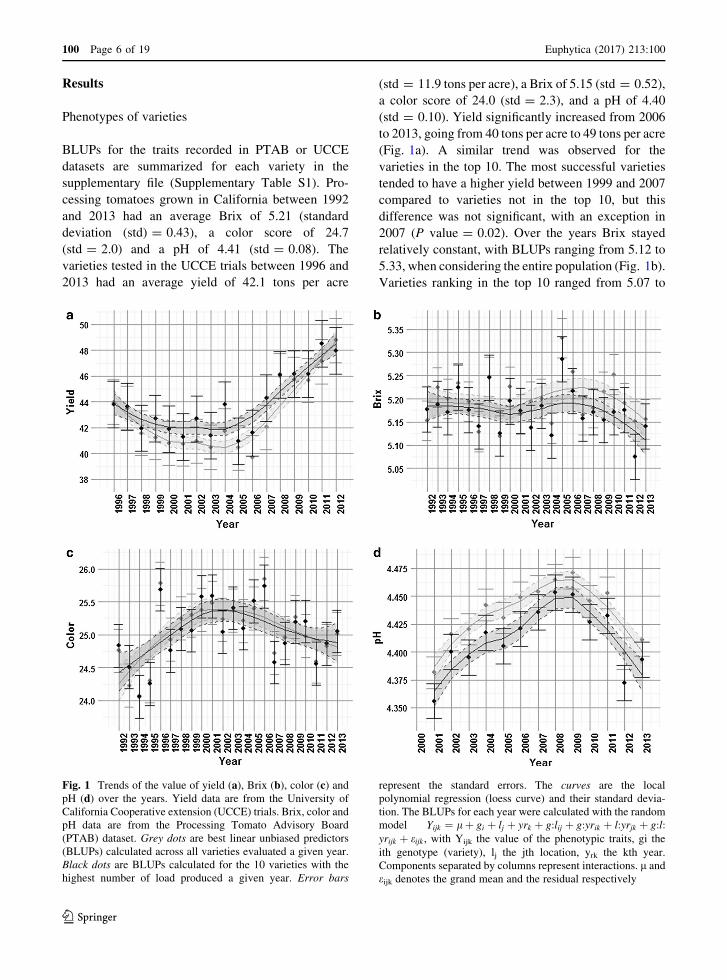
(std = 0.10). Yield significantly increased from 2006
to 2013, going from 40 tons per acre to 49 tons per acre
(Fig. 1a). A similar trend was observed for the
varieties in the top 10. The most successful varieties
tended to have a higher yield between 1999 and 2007
compared to varieties not in the top 10, but this
difference was not significant, with an exception in
2007 (P value = 0.02). Over the years Brix stayed
relatively constant, with BLUPs ranging from 5.12 to
5.33, when considering the entire population (Fig. 1b).
Varieties ranking in the top 10 ranged from 5.07 to
Fig. 1 Trends of the value of yield (a), Brix (b), color (c) andpH (d) over the years. Yield data are from the University of
California Cooperative extension (UCCE) trials. Brix, color and
pH data are from the Processing Tomato Advisory Board
(PTAB) dataset. Grey dots are best linear unbiased predictors
(BLUPs) calculated across all varieties evaluated a given year.
Black dots are BLUPs calculated for the 10 varieties with the
highest number of load produced a given year. Error bars
represent the standard errors. The curves are the local
polynomial regression (loess curve) and their standard devia-
tion. The BLUPs for each year were calculated with the random
model Yijk ¼ lþ gi þ lj þ yrk þ g:lij þ g:yrik þ l:yrjk þ g:l:yrijk þ eijk , with Yijk the value of the phenotypic traits, gi the
ith genotype (variety), lj the jth location, yrk the kth year.
Components separated by columns represent interactions. l and
eijk denotes the grand mean and the residual respectively
100 Page 6 of 19 Euphytica (2017) 213:100
123
5.29, and tended to have lower Brix than the rest of the
population (Fig. 1b), but this difference was not
significant. BLUPs of color scores ranged from 24.1
to 25.8, with lower values before 1995 (Fig. 1c). A
similar trend was observed for varieties from the top
10 (Fig. 1c). BLUPs for pH calculated for each year
showed an increase from 4.38 (2001) to 4.47 (2009),
followed by a decrease, with values reaching 4.40 in
2012 (Fig. 1d). Varieties ranking in the top 10 showed
a BLUP for pH that was consistently lower by
0.02–0.03 units compared to the entire population.
Varieties ranking in the top 10 had a significantly
lower pH than the other varieties in 2007 and from
2010 to 2012 (P-value from 0.01 to 0.05) (Fig. 1d).
Data for disease resistances was found for 216
varieties out of the 927 varieties in the PTAB dataset.
The resistances reported the most frequently by seed
companies were for root knock nematode (Mi),
bacterial speck (Pto), Verticilium race I, Fusarium
wilt races I and II, tomato spotted wilt virus (TSWV),
and bacterial canker (partial resistance). More rarely,
resistances to bacterial spot (partial resistance), grey
leaf spot (partial resistance), tobacco mosaic virus
(Tm2a), Fusarium wilt race III, and dodder (partial
resistance) were reported. Varieties included from two
to six resistances. On average, over the entire popu-
lation, a variety had 3.8 resistances. The average
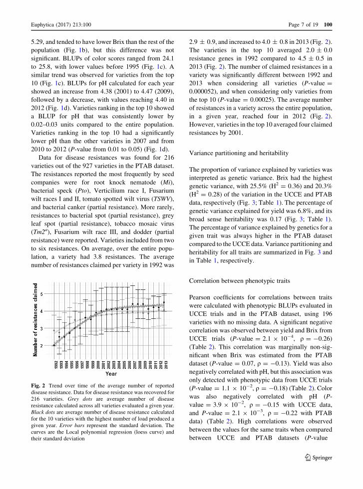
number of resistances claimed per variety in 1992 was
2.9 ± 0.9, and increased to 4.0 ± 0.8 in 2013 (Fig. 2).
The varieties in the top 10 averaged 2.0 ± 0.0
resistance genes in 1992 compared to 4.5 ± 0.5 in
2013 (Fig. 2). The number of claimed resistances in a
variety was significantly different between 1992 and
2013 when considering all varieties (P-value =
0.000052), and when considering only varieties from
the top 10 (P-value = 0.00025). The average number
of resistances in a variety across the entire population,
in a given year, reached four in 2012 (Fig. 2).
However, varieties in the top 10 averaged four claimed
resistances by 2001.
Variance partitioning and heritability
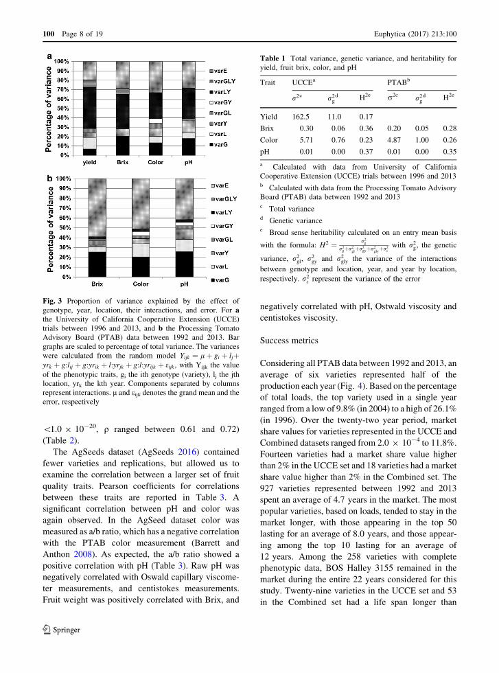
The proportion of variance explained by varieties was
interpreted as genetic variance. Brix had the highest
genetic variance, with 25.5% (H2 = 0.36) and 20.3%
(H2 = 0.28) of the variation in the UCCE and PTAB
data, respectively (Fig. 3; Table 1). The percentage of
genetic variance explained for yield was 6.8%, and its
broad sense heritability was 0.17 (Fig. 3; Table 1).
The percentage of variance explained by genetics for a
given trait was always higher in the PTAB dataset
compared to the UCCE data. Variance partitioning and
heritability for all traits are summarized in Fig. 3 and
in Table 1, respectively.
Correlation between phenotypic traits
Pearson coefficients for correlations between traits
were calculated with phenotypic BLUPs evaluated in
UCCE trials and in the PTAB dataset, using 196
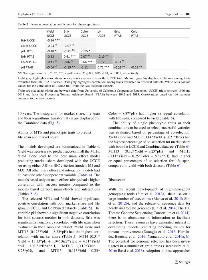
varieties with no missing data. A significant negative
correlation was observed between yield and Brix from
UCCE trials (P-value = 2.1 9 10-4, q = -0.26)
(Table 2). This correlation was marginally non-sig-
nificant when Brix was estimated from the PTAB
dataset (P-value = 0.07, q = -0.13). Yield was also
negatively correlated with pH, but this association was
only detected with phenotypic data from UCCE trials
(P-value = 1.1 9 10-2, q = -0.18) (Table 2). Color
was also negatively correlated with pH (P-
value = 3.9 9 10-2, q = -0.15 with UCCE data,
and P-value = 2.1 9 10-3, q = -0.22 with PTAB
data) (Table 2). High correlations were observed
between the values for the same traits when compared
between UCCE and PTAB datasets (P-value
Fig. 2 Trend over time of the average number of reported
disease resistance. Data for disease resistance was recovered for
216 varieties. Grey dots are average number of disease
resistance calculated across all varieties evaluated a given year.
Black dots are average number of disease resistance calculated
for the 10 varieties with the highest number of load produced a
given year. Error bars represent the standard deviation. The
curves are the Local polynomial regression (loess curve) and
their standard deviation
Euphytica (2017) 213:100 Page 7 of 19 100
123
\1.0 9 10-20, q ranged between 0.61 and 0.72)
(Table 2).
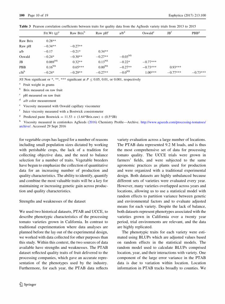
The AgSeeds dataset (AgSeeds 2016) contained
fewer varieties and replications, but allowed us to
examine the correlation between a larger set of fruit
quality traits. Pearson coefficients for correlations
between these traits are reported in Table 3. A
significant correlation between pH and color was
again observed. In the AgSeed dataset color was
measured as a/b ratio, which has a negative correlation
with the PTAB color measurement (Barrett and
Anthon 2008). As expected, the a/b ratio showed a
positive correlation with pH (Table 3). Raw pH was
negatively correlated with Oswald capillary viscome-
ter measurements, and centistokes measurements.
Fruit weight was positively correlated with Brix, and
negatively correlated with pH, Ostwald viscosity and
centistokes viscosity.
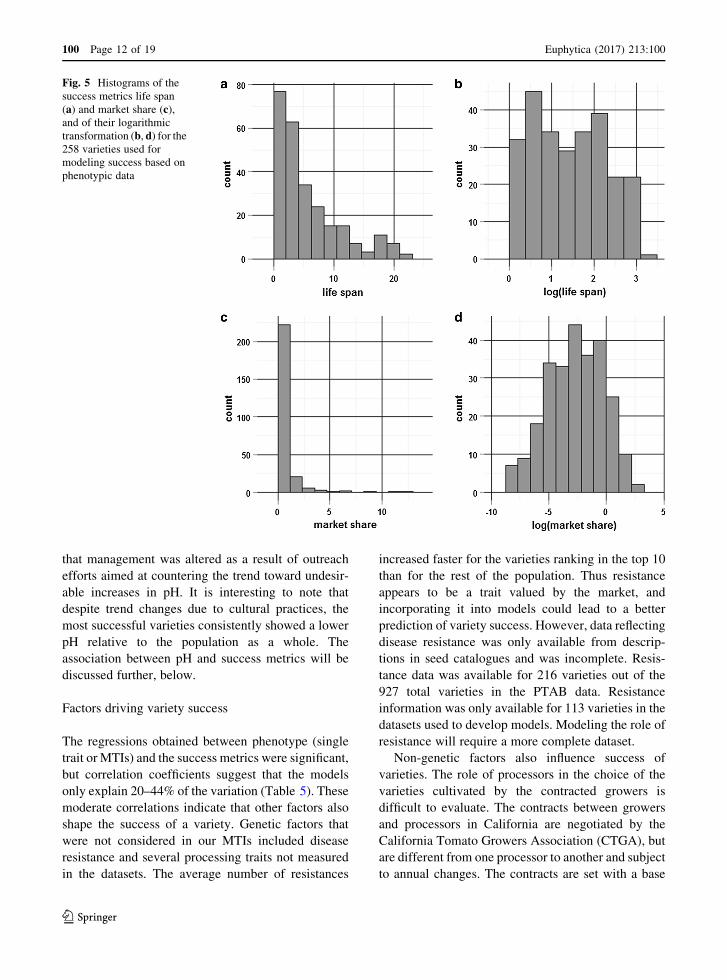
Success metrics
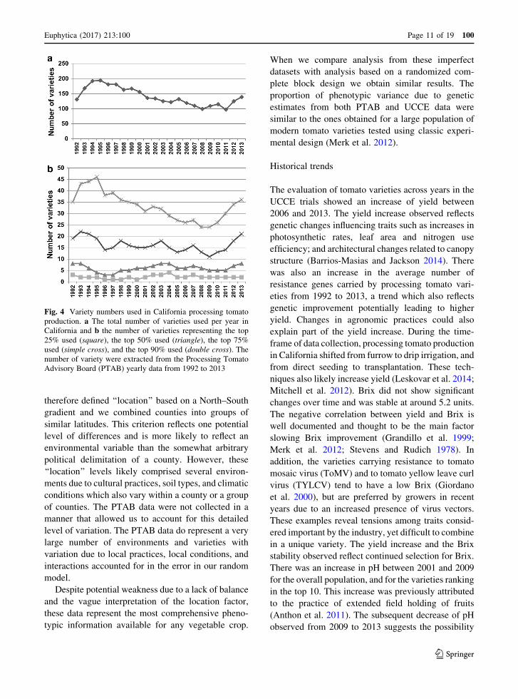
Considering all PTAB data between 1992 and 2013, an
average of six varieties represented half of the
production each year (Fig. 4). Based on the percentage
of total loads, the top variety used in a single year
ranged from a low of 9.8% (in 2004) to a high of 26.1%
(in 1996). Over the twenty-two year period, market
share values for varieties represented in the UCCE and
Combined datasets ranged from 2.0 9 10-4 to 11.8%.
Fourteen varieties had a market share value higher
than 2% in the UCCE set and 18 varieties had a market
share value higher than 2% in the Combined set. The
927 varieties represented between 1992 and 2013
spent an average of 4.7 years in the market. The most
popular varieties, based on loads, tended to stay in the
market longer, with those appearing in the top 50
lasting for an average of 8.0 years, and those appear-
ing among the top 10 lasting for an average of
12 years. Among the 258 varieties with complete
phenotypic data, BOS Halley 3155 remained in the
market during the entire 22 years considered for this
study. Twenty-nine varieties in the UCCE set and 53
in the Combined set had a life span longer than
Fig. 3 Proportion of variance explained by the effect of
genotype, year, location, their interactions, and error. For athe University of California Cooperative Extension (UCCE)
trials between 1996 and 2013, and b the Processing Tomato
Advisory Board (PTAB) data between 1992 and 2013. Bar
graphs are scaled to percentage of total variance. The variances
were calculated from the random model Yijk ¼ lþ gi þ ljþyrk þ g:lij þ g:yrik þ l:yrjk þ g:l:yrijk þ eijk , with Yijk the value
of the phenotypic traits, gi the ith genotype (variety), lj the jth
location, yrk the kth year. Components separated by columns
represent interactions. l and eijk denotes the grand mean and the
error, respectively
Table 1 Total variance, genetic variance, and heritability for
yield, fruit brix, color, and pH
Trait UCCEa PTABb
r2c r2gd H2e r2c r2g
d H2e
Yield 162.5 11.0 0.17
Brix 0.30 0.06 0.36 0.20 0.05 0.28
Color 5.71 0.76 0.23 4.87 1.00 0.26
pH 0.01 0.00 0.37 0.01 0.00 0.35
a Calculated with data from University of California
Cooperative Extension (UCCE) trials between 1996 and 2013b Calculated with data from the Processing Tomato Advisory
Board (PTAB) data between 1992 and 2013c Total varianced Genetic variancee Broad sense heritability calculated on an entry mean basis
with the formula: H2 ¼ r2gr2gþr2
glþr2gyþr2
glyþr2e
with r2g, the genetic
variance, r2gl, r2gy and r2gly the variance of the interactions
between genotype and location, year, and year by location,
respectively. r2e represent the variance of the error
100 Page 8 of 19 Euphytica (2017) 213:100
123
10 years. The histograms for market share, life span
and their logarithmic transformation are displayed for
the Combined data (Fig. 5).
Ability of MTIs and phenotypic traits to predict
life span and market share
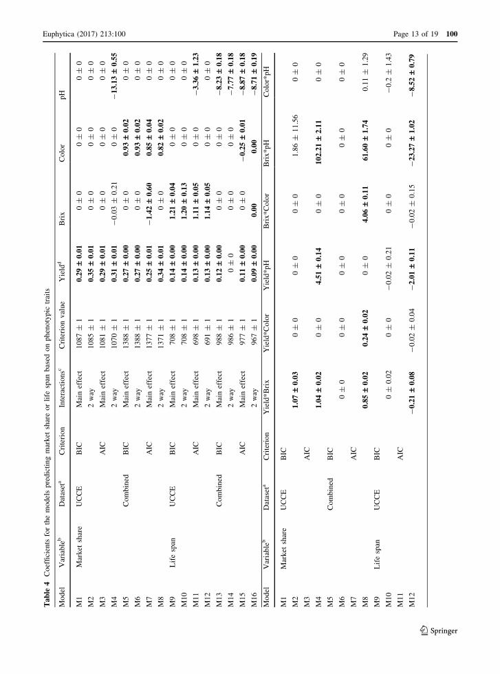
The models developed are summarized in Table 4.
Yield was necessary to predict success in all the MTIs.
Yield alone lead to the best main effect model
predicting market share developed with the UCCE
set using either AIC or BIC criterion (models M1 and
M3). All other main effect and interaction models had
at least one other independent variable (Table 4). The
models based only onmain effects always had a higher
correlation with success metrics compared to the
models based on both main effects and interactions
(Tables 5, 6).
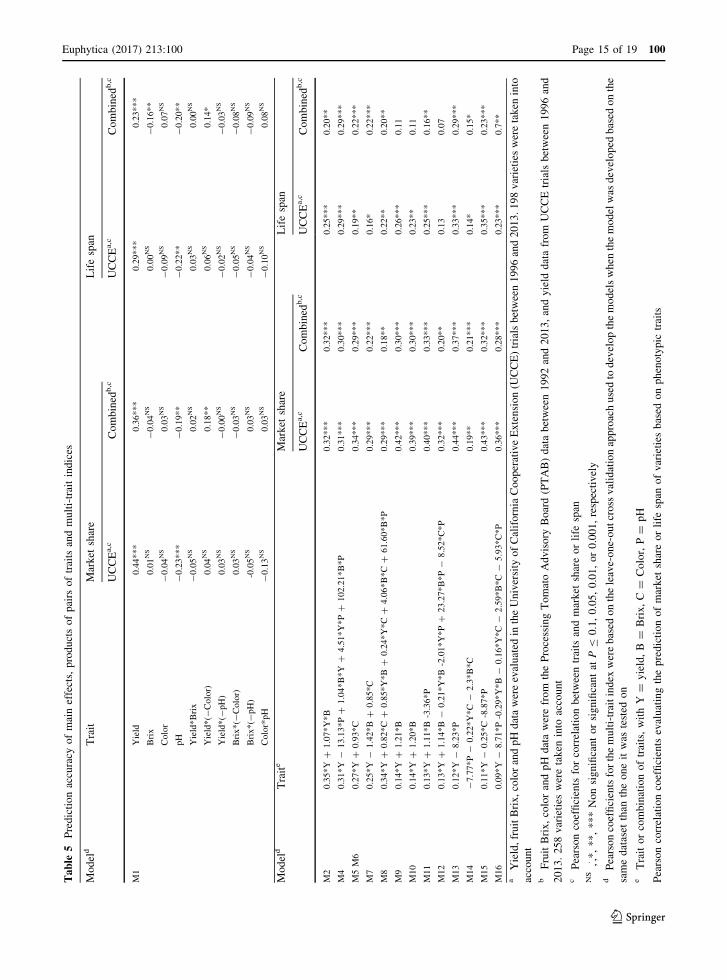
The selected MTIs and Yield showed significant
positive correlation with both market share and life
span, in UCCE and Combined datasets (Table 5). The
variable pH showed a significant negative correlation
for both success metrics in both datasets. Brix was
significantly negatively correlated with life span when
evaluated in the Combined dataset. Yield alone and
MTI13 (0.12*Yield - 8.23*pH) had the highest cor-
relation with market share (Table 5). MTI4 (0.31*
Yield - 13.13*pH ? 1.04*Brix*Yield ? 4.51*Yield
*pH ? 102.21*Brix*pH), MTI13 (0.12*Yield -
8.23*pH), and MTI15 (0.11*Yield - 0.25*
Color - 8.87*pH) had higher or equal correlation
with life span, compared to yield (Table 5).
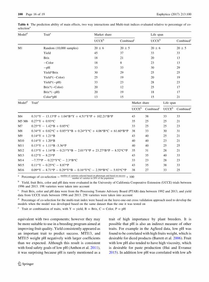
The ability of single phenotypic traits or their
combinations to be used to select successful varieties
was evaluated based on percentage of co-selection.
Yield alone and MTI9 (0.14*Yield ? 1.21*Brix) had
the highest percentage of co-selection for market share
with both the UCCE and Combined datasets (Table 6).
MTI13 (0.12*Yield - 8.23*pH) and MTI15
(0.11*Yield - 0.25*Color - 8.87*pH) had higher
or equal percentages of co-selection for life span,
compared to yield with both datasets (Table 6).
Discussion
With the recent development of high-throughput
genotyping tools (Sim et al. 2012a), their use on a
large number of accessions (Blanca et al. 2015; Sim
et al. 2012b), and the release of sequence data for
nearly 440 tomato genomes (Lin et al. 2014; The 100
Tomato Genome Sequencing Consortium et al. 2014),
there is an abundance of information to facilitate
selection. These resources have generated interest in
developing models predicting breeding values for
tomato improvement (Duangjit et al. 2016; Hernan-
dez-Bautista et al. 2016; Yamamoto et al. 2016a, b).
The potential for genomic selection has been inves-
tigated in a number of grain crops (Barabaschi et al.
2016; Bassi et al. 2016). Adoption of these approaches
Table 2 Pearson correlation coefficients for phenotypic traits
Yield UCCE
Brix UCCE
Color UCCE
pH UCCE
Brix PTAB
Color PTAB
Brix UCCE -0.26 ***Color UCCE -0.04 NS -0.07 NS
pH UCCE -0.18 * -0.11 NS -0.15 *Brix PTAB -0.13 . 0.61 *** 0.07 NS -0.19 **Color PTAB -0.11 NS 0.06 NS 0.66 *** -0.12 . -0.11 NS
pH PTAB -0.06 NS -0.19 ** -0.12 . 0.72 *** -0.21 ** -0.22 **
NS Non significant or �, *, **, *** significant at P B 0.1, 0.05, 0.01, or 0.001, respectively
Light gray highlights correlations among traits evaluated from the UCCE trial. Medium gray highlights correlations among traits
evaluated from the PTAB dataset. Dark gray highlights correlation among traits evaluated in different datasets. White cells contain
values for the correlation of a same trait from the two different datasets
Traits are evaluated within and between data from University of California Cooperative Extension (UCCE) trials between 1996 and
2013 and from the Processing Tomato Advisory Board (PTAB) between 1992 and 2013. Observations based on 196 varieties
common to the two datasets
Euphytica (2017) 213:100 Page 9 of 19 100
123
for vegetable crops has lagged for a number of reasons
including small population sizes dictated by working
with perishable crops, the lack of a tradition for
collecting objective data, and the need to balance
selection for a number of traits. Vegetable breeders
have begun to emphasize the collection of quantitative
data for an increasing number of production and
quality characteristics. The ability to identify, quantify
and combine the most valuable traits will be a key for
maintaining or increasing genetic gain across produc-
tion and quality characteristics.
Strengths and weaknesses of the dataset
We used two historical datasets, PTAB and UCCE, to
describe phenotypic characteristics of the processing
tomato varieties grown in California. In contrast to
traditional experimentation where data analyses are
planned before the lay out of the experimental design,
we worked with data collected for other purposes than
this study. Within this context, the two sources of data
available have strengths and weaknesses. The PTAB
dataset reflected quality traits of fruit delivered to the
processing companies, which gave an accurate repre-
sentation of the phenotypes used by the industry.
Furthermore, for each year, the PTAB data reflects
variety evaluation across a large number of locations.
The PTAB data represented 9.2 M loads, and is thus
the most comprehensive set of data for processing
tomato quality. The UCCE trials were grown in
farmers’ fields, and were subjected to the same
agronomic practices as plants used for production
and were organized with a traditional experimental
design. Both datasets are highly unbalanced because
different sets of varieties were evaluated every year.
However, many varieties overlapped across years and
locations, allowing us to use a statistical model with
random effects to partition variance between genetic
and environmental factors and to evaluate adjusted
means for each variety. Despite the lack of balance,
both datasets represent phenotypes associated with the
varieties grown in California over a twenty year
period, trial environments are relevant, and the data
are highly replicated.
The phenotypic traits for each variety were esti-
mated using BLUPs which are adjusted values based
on random effects in the statistical models. The
random model used to calculate BLUPs comprised
location, year, and their interactions with variety. One
component of the large error variance in the PTAB
data is due to variation within location. Location
information in PTAB tracks broadly to counties. We
Table 3 Pearson correlation coefficients between traits for quality data from the AgSeeds variety trials from 2013 to 2015
Frt.Wt (g)a Raw Brixb Raw pHc a/bd Oswalde JBf PBBg
Raw Brix 0.28**
Raw pH -0.34** -0.27**
a/b -0.17 -0.21* 0.34**
Oswald -0.24* -0.30** -0.27** -0.03NS
JB 0.069NS 0.32** 0.13NS -0.22* -0.77***
PBB 0.16NS 0.65*** 0.00NS -0.27** -0.73*** 0.93***
cSth -0.24* -0.29** -0.27** -0.0NS 1.00*** -0.77*** -0.73***
NS Non significant or *, **, *** significant at P B 0.05, 0.01, or 0.001, respectivelya Fruit weight in gramsb Brix measured on raw fruitc pH measured on raw fruitd a/b color measuremente Viscosity measured with Oswald capillary viscometerf Juice viscosity measured with a Bostwick consistometerg Predicted paste Bostwick = 11.53 ? (1.64*Brix.raw) ? (0.5*JB)h Viscosity measured in centistokes AgSeeds (2016) Chemistry Profile—Archive. http://www.agseeds.com/processing-tomatoes/
archive/. Accessed 29 Sept 2016
100 Page 10 of 19 Euphytica (2017) 213:100
123
therefore defined ‘‘location’’ based on a North–South
gradient and we combined counties into groups of
similar latitudes. This criterion reflects one potential
level of differences and is more likely to reflect an
environmental variable than the somewhat arbitrary
political delimitation of a county. However, these
‘‘location’’ levels likely comprised several environ-
ments due to cultural practices, soil types, and climatic
conditions which also vary within a county or a group
of counties. The PTAB data were not collected in a
manner that allowed us to account for this detailed
level of variation. The PTAB data do represent a very
large number of environments and varieties with
variation due to local practices, local conditions, and
interactions accounted for in the error in our random
model.
Despite potential weakness due to a lack of balance
and the vague interpretation of the location factor,
these data represent the most comprehensive pheno-
typic information available for any vegetable crop.
When we compare analysis from these imperfect
datasets with analysis based on a randomized com-
plete block design we obtain similar results. The
proportion of phenotypic variance due to genetic
estimates from both PTAB and UCCE data were
similar to the ones obtained for a large population of
modern tomato varieties tested using classic experi-
mental design (Merk et al. 2012).
Historical trends
The evaluation of tomato varieties across years in the
UCCE trials showed an increase of yield between
2006 and 2013. The yield increase observed reflects
genetic changes influencing traits such as increases in
photosynthetic rates, leaf area and nitrogen use
efficiency; and architectural changes related to canopy
structure (Barrios-Masias and Jackson 2014). There
was also an increase in the average number of
resistance genes carried by processing tomato vari-
eties from 1992 to 2013, a trend which also reflects
genetic improvement potentially leading to higher
yield. Changes in agronomic practices could also
explain part of the yield increase. During the time-
frame of data collection, processing tomato production
in California shifted from furrow to drip irrigation, and
from direct seeding to transplantation. These tech-
niques also likely increase yield (Leskovar et al. 2014;
Mitchell et al. 2012). Brix did not show significant
changes over time and was stable at around 5.2 units.
The negative correlation between yield and Brix is
well documented and thought to be the main factor
slowing Brix improvement (Grandillo et al. 1999;
Merk et al. 2012; Stevens and Rudich 1978). In
addition, the varieties carrying resistance to tomato
mosaic virus (ToMV) and to tomato yellow leave curl
virus (TYLCV) tend to have a low Brix (Giordano
et al. 2000), but are preferred by growers in recent
years due to an increased presence of virus vectors.
These examples reveal tensions among traits consid-
ered important by the industry, yet difficult to combine
in a unique variety. The yield increase and the Brix
stability observed reflect continued selection for Brix.
There was an increase in pH between 2001 and 2009
for the overall population, and for the varieties ranking
in the top 10. This increase was previously attributed
to the practice of extended field holding of fruits
(Anthon et al. 2011). The subsequent decrease of pH
observed from 2009 to 2013 suggests the possibility
Fig. 4 Variety numbers used in California processing tomato
production. a The total number of varieties used per year in
California and b the number of varieties representing the top
25% used (square), the top 50% used (triangle), the top 75%
used (simple cross), and the top 90% used (double cross). The
number of variety were extracted from the Processing Tomato
Advisory Board (PTAB) yearly data from 1992 to 2013
Euphytica (2017) 213:100 Page 11 of 19 100
123
that management was altered as a result of outreach
efforts aimed at countering the trend toward undesir-
able increases in pH. It is interesting to note that
despite trend changes due to cultural practices, the
most successful varieties consistently showed a lower
pH relative to the population as a whole. The
association between pH and success metrics will be
discussed further, below.
Factors driving variety success
The regressions obtained between phenotype (single
trait or MTIs) and the success metrics were significant,
but correlation coefficients suggest that the models
only explain 20–44% of the variation (Table 5). These
moderate correlations indicate that other factors also
shape the success of a variety. Genetic factors that
were not considered in our MTIs included disease
resistance and several processing traits not measured
in the datasets. The average number of resistances
increased faster for the varieties ranking in the top 10
than for the rest of the population. Thus resistance
appears to be a trait valued by the market, and
incorporating it into models could lead to a better
prediction of variety success. However, data reflecting
disease resistance was only available from descrip-
tions in seed catalogues and was incomplete. Resis-
tance data was available for 216 varieties out of the
927 total varieties in the PTAB data. Resistance
information was only available for 113 varieties in the
datasets used to develop models. Modeling the role of
resistance will require a more complete dataset.
Non-genetic factors also influence success of
varieties. The role of processors in the choice of the
varieties cultivated by the contracted growers is
difficult to evaluate. The contracts between growers
and processors in California are negotiated by the
California Tomato Growers Association (CTGA), but
are different from one processor to another and subject
to annual changes. The contracts are set with a base
Fig. 5 Histograms of the
success metrics life span
(a) and market share (c),and of their logarithmic
transformation (b, d) for the258 varieties used for
modeling success based on
phenotypic data
100 Page 12 of 19 Euphytica (2017) 213:100
123
Table
4Coefficients
forthemodelspredictingmarket
shareorlife
span
based
onphenotypic
traits
Model
Variableb
Dataseta
Criterion
Interactionsc
Criterionvalue
Yield
dBrix
Color
pH
M1
Market
share
UCCE
BIC
Maineffect
1087±
10.29–0.01
0±
00±
00±
0
M2
2way
1085±
10.35–0.01
0±
00±
00±
0
M3
AIC
Maineffect
1081±
10.29–0.01
0±
00±
00±
0
M4
2way
1070±
10.31–0.01
-0.03±
0.21
0±
0-13.13–0.55
M5
Combined
BIC
Maineffect
1388±
10.27–0.00
0±
00.93–0.02
0±
0
M6
2way
1388±
10.27–0.00
0±
00.93–0.02
0±
0
M7
AIC
Maineffect
1377±
10.25–0.01
-1.42–0.60
0.85–0.04
0±
0
M8
2way
1371±
10.34–0.01
0±
00.82–0.02
0±
0
M9
Lifespan
UCCE
BIC
Maineffect
708±
10.14–0.00
1.21–0.04
0±
00±
0
M10
2way
708±
10.14–0.00
1.20–0.13
0±
00±
0
M11
AIC
Maineffect
698±
10.13–0.00
1.11–0.05
0±
0-3.36–1.23
M12
2way
691±
10.13–0.00
1.14–0.05
0±
00±
0
M13
Combined
BIC
Maineffect
988±
10.12–0.00
0±
00±
0-8.23–0.18
M14
2way
986±
10±
00±
00±
0-7.77–0.18
M15
AIC
Maineffect
977±
10.11–0.00
0±
0-0.25–0.01
-8.87–0.18
M16
2way
967±
10.09–0.00
0.00
0.00
-8.71–0.19
Model
Variableb
Dataseta
Criterion
Yield*Brix
Yield*Color
Yield*pH
Brix*Color
Brix*pH
Color*pH
M1
Market
share
UCCE
BIC
M2
1.07–0.03
0±
00±
00±
01.86±
11.56
0±
0
M3
AIC
M4
1.04–0.02
0±
04.51–0.14
0±
0102.21–2.11
0±
0
M5
Combined
BIC
M6
0±
00±
00±
00±
00±
00±
0
M7
AIC
M8
0.85–0.02
0.24–0.02
0±
04.06–0.11
61.60–1.74
0.11±
1.29
M9
Lifespan
UCCE
BIC
M10
0±
0.02
0±
0-0.02±
0.21
0±
00±
0-0.2
±1.43
M11
AIC
M12
-0.21–0.08
-0.02±
0.04
-2.01–0.11
-0.02±
0.15
-23.27–1.02
-8.52–0.79
Euphytica (2017) 213:100 Page 13 of 19 100
123

price per ton, with a linear deduction or increase
depending on quality criteria (Hueth and Ligon 2002).
Contracts have an impact on both the agricultural
techniques used by the farmers, and on the varieties
grown (Alexander et al. 2007). The contracts are
confidential, thus it is difficult to use these documents
to weigh traits in the context of a breeding program.
Similarly, the human factors involved in variety
choices, such as trust in a given brand or company,
are difficult to evaluate. As evidence of confounding
effects, market share was significantly associated with
seed company (Kruskal–Wallis test, P-
value = 6.0 9 10-8) (Table S1). In addition process-
ing tomato varieties can be divided into several
categories based on their properties and use, such as
multiuse, solid, and viscosity (Gould 1992; Stevens
and Rick 1986). The market share or life span of a
variety could be influenced by its market category,
particularly for the categories representing niches for
the industry. Processing categories were not available
for all varieties, and most of the varieties for which we
recovered this information were classified as multi-use
(83%). Thus the MTIs represent the processing tomato
market regardless of the variety categories, and should
be considered a multi-use index.
Weights of the multi trait indices
Yield alone ranked among the highest indices for
ability to predict variety success in the market. This
observation confirms that yield has been the main
driver of variety success. The equation Y9B has been
suggested to balance selection for two important traits
(Eshed et al. 1996; Grandillo et al. 1999; Tanksley
et al. 1996). However, the value of this equation does
not significantly correlate with variety success
(Table 5). The YxB index demonstrated a percentage
of co-selection higher than for a random sample, but
lower than yield alone and lower than the best MTIs
we developed (Table 6).
Three of the MTIs we developed predicted success
of varieties with approximately the same or better
accuracy than yield alone. The use of these MTIs in
breeding programs could increase genetic gains for
fruit quality traits. These MTIs were MTI9 [0.14*
yield ? 1.21*Brix], MTI13 [0.12*Yield - 8.23*pH],
and MTI15 [0.11*Yield - 0.25*Color - 8.87*pH].
MTIs with three or more components have a slightly
lower ability to predict success compared to theirTable
4continued
Model
Variableb
Dataseta
Criterion
Yield*Brix
Yield*Color
Yield*pH
Brix*Color
Brix*pH
Color*pH
M13
Combined
BIC
M14
0±
0-0.22–0.00
0±
0-2.3
–0.05
0±
00±
0
M15
AIC
M16
-0.29–0.02
-0.16–0.00
0±
0-2.59–0.06
0±
0-5.93–1.08
Theequationsweredeveloped
withgenerallinearmodelsbased
onBayesianinform
ationCriteria(BIC).Aleave-oneoutcross
validationwas
used,andtheresultspresentedhere
aremeansandstandarddeviationsofthecoefficients
obtained
across
repetitionsfrom
thecross
validation
a‘‘UCCE’’denotesmodel
developed
withphenotypic
datafrom
theUniversity
ofCalifornia
CooperativeExtensiontrials
(UCCE)between1996and2013,containing198
varieties.‘‘Combined’’denotesmodelsdeveloped
withphenotypicdataforfruitBrix,colorandpHfrom
theProcessingTomatoAdvisory
Board(PTAB)databetween1992and
2013,andyield
datafrom
theUCCEtrials
between1996and2013,containing258varieties
bThevariable
market
shareandlife
span
wheretransform
edwithalogarithmic
function(log(e))
cTheinitialequationsused
forthemodeling
process
wereeither
successvariable
=Yield
?Brix?
Color?
pH
(no
interactions)
orsuccessvariable
=Yield
?Brix?
Color?
pH
?Yield*Brix?
Yield*Color?
Yield*pH
?Brix*Color?
Brix*pH
?Color*pH(2way
interactions).Independentvariables(phenotypictraits)withcoefficientsof0±
0
didnotcontributetothefitofthemodelbased
onan
exhaustiveapproach(m
odelwithsm
allestBIC
amongallpossiblemodels)im
plementedintheglm
ultifunctioninR
dThebold
componentsoftheequationswereconsidered
forthemulti-traitindices.Coefficientswithstandarddeviationslarger
than
themeanswereelim
inated
from
themulti-
traitindices
(notbolded)
100 Page 14 of 19 Euphytica (2017) 213:100
123
Table
5Predictionaccuracy
ofmaineffects,productsofpairs
oftraits
andmulti-traitindices
Modeld
Trait
Market
share
Lifespan
UCCEa,c
Combined
b,c
UCCEa,c
Combined
b,c
M1
Yield
0.44***
0.36***
0.29***
0.23***
Brix
0.01NS
-0.04NS
0.00NS
-0.16**
Color
-0.04NS
0.03NS
-0.09NS
0.07NS
pH
-0.23***
-0.19**
-0.22**
-0.20**
Yield*Brix
-0.05NS
0.02NS
0.03NS
0.00NS
Yield*(-
Color)
0.04NS
0.18**
0.06NS
0.14*
Yield*(-
pH)
0.03NS
-0.00NS
-0.02NS
-0.03NS
Brix*(-
Color)
0.03NS
-0.03NS
-0.05NS
-0.08NS
Brix*(-
pH)
-0.05NS
0.03NS
-0.04NS
-0.09NS
Color*pH
-0.13NS
0.03NS
-0.10NS
0.08NS
Modeld
Traite
Market
share
Lifespan
UCCEa,c
Combined
b,c
UCCEa,c
Combined
b,c
M2
0.35*Y
?1.07*Y*B
0.32***
0.32***
0.25***
0.20**
M4
0.31*Y
-13.13*P?
1.04*B*Y
?4.51*Y*P?
102.21*B*P
0.31***
0.30***
0.29***
0.29***
M5M6
0.27*Y
?0.93*C
0.34***
0.29***
0.19**
0.22***
M7
0.25*Y
-1.42*B
?0.85*C
0.29***
0.22***
0.16*
0.22***
M8
0.34*Y
?0.82*C
?0.85*Y*B
?0.24*Y*C
?4.06*B*C?
61.60*B*P
0.29***
0.18**
0.22**
0.20**
M9
0.14*Y
?1.21*B
0.42***
0.30***
0.26***
0.11
M10
0.14*Y
?1.20*B
0.39***
0.30***
0.23**
0.11
M11
0.13*Y
?1.11*B
-3.36*P
0.40***
0.33***
0.25***
0.16**
M12
0.13*Y
?1.14*B
-0.21*Y*B
-2.01*Y*P?
23.27*B*P-
8.52*C*P
0.32***
0.20**
0.13
0.07
M13
0.12*Y
-8.23*P
0.44***
0.37***
0.33***
0.29***
M14
-7.77*P-
0.22*Y*C
-2.3*B*C
0.19**
0.21***
0.14*
0.15*
M15
0.11*Y
-0.25*C
-8.87*P
0.43***
0.32***
0.35***
0.23***
M16
0.09*Y
-8.71*P-0.29*Y*B
-0.16*Y*C
-2.59*B*C
-5.93*C*P
0.36***
0.28***
0.23***
0.7**
aYield,fruitBrix,colorandpHdatawereevaluated
intheUniversity
ofCaliforniaCooperativeExtension(U
CCE)trialsbetween1996and2013.198varieties
weretaken
into
account
bFruitBrix,colorandpH
datawerefrom
theProcessingTomatoAdvisory
Board(PTAB)databetween1992and2013,andyield
datafrom
UCCEtrialsbetween1996and
2013.258varieties
weretaken
into
account
cPearsoncoefficients
forcorrelationbetweentraits
andmarket
shareorlife
span
NS,� ,*,**,***Nonsignificantorsignificantat
PB
0.1,0.05,0.01,or0.001,respectively
dPearsoncoefficientsforthemulti-traitindex
werebased
ontheleave-one-outcross
validationapproachusedto
developthemodelswhen
themodelwas
developed
based
onthe
samedataset
than
theoneitwas
tested
on
eTraitorcombinationoftraits,withY
=yield,B=
Brix,C=
Color,P=
pH
Pearsoncorrelationcoefficients
evaluatingthepredictionofmarket
shareorlife
span
ofvarieties
based
onphenotypic
traits
Euphytica (2017) 213:100 Page 15 of 19 100
123
equivalent with two components; however they may
be more suitable to use in a breeding program aimed at
improving fruit quality. Yield consistently appeared as
an important trait to predict success. MTI13, and
MTI15 weight pH negatively with larger coefficients
than we expected. Although this result is consistent
with food safety goals of low pH (Anthon et al. 2011),
it was surprising because pH is rarely mentioned as a
trait of high importance by plant breeders. It is
possible that pH is also an indirect measure of other
traits. For example in the AgSeed data, low pH was
found to be correlated with high fruits weight, which is
desirable for diced products (Barrett et al. 2006). Fruit
with low pH also tended to have high viscosity, which
is desirable for paste production (Hui and Evranuz
2015). In addition low pH was correlated with low a/b
Table 6 The prediction ability of main effects, two way interactions and Multi-trait indices evaluated relative to percentage of co-
selectiona
Modeld Traite Market share Life span
UCCEb Combinedc UCCEb Combinedc
M1 Random (10,000 samples) 20 ± 6 20 ± 5 20 ± 6 20 ± 5
Yield 45 37 33 33
Brix 18 21 20 13
-Color 18 8 23 13
-pH 33 33 30 29
Yield*Brix 30 29 25 25
Yield*(-Color) 25 19 20 19
Yield*(-pH) 33 23 28 23
Brix*(-Color) 20 12 25 17
Brix*(-pH) 20 19 18 17
Color*pH 13 15 15 21
Modeld Traite Market share Life span
UCCEb Combinedc UCCEb Combinedc
M4 0.31*Y - 13.13*P ? 1.04*B*Y ? 4.51*Y*P ? 102.21*B*P 43 38 33 33
M5 M6 0.27*Y ? 0.93*C 35 25 25 21
M7 0.25*Y - 1.42*B ? 0.85*C 33 25 25 23
M8 0.34*Y ? 0.82*C ? 0.85*Y*B ? 0.24*Y*C ? 4.06*B*C ? 61.60*B*P 38 33 30 31
M9 0.14*Y ? 1.21*B 43 40 25 21
M10 0.14*Y ? 1.20*B 40 40 23 21
M11 0.13*Y ? 1.11*B -3.36*P 40 40 25 25
M12 0.13*Y ? 1.14*B - 0.21*Y*B - 2.01*Y*P ? 23.27*B*P - 8.52*C*P 35 31 28 21
M13 0.12*Y - 8.23*P 43 35 40 33
M14 -7.77*P - 0.22*Y*C - 2.3*B*C 33 23 28 23
M15 0.11*Y - 0.25*C - 8.87*P 43 35 38 33
M16 0.09*Y - 8.71*P - 0.29*Y*B - 0.16*Y*C - 2.59*B*C - 5.93*C*P 38 27 33 25
a Percentage of co-selection ¼ number of varieties selected based on phenotype and based on successnumber of varieties in 20% of the population
� 100
b Yield, fruit Brix, color and pH data were evaluated in the University of California Cooperative Extension (UCCE) trials between
1996 and 2013. 198 varieties were taken into accountc Fruit Brix, color and pH data were from the Processing Tomato Advisory Board (PTAB) data between 1992 and 2013, and yield
data from UCCE trials between 1996 and 2013. 258 varieties were taken into accountd Percentage of co-selection for the multi-trait index were based on the leave-one-out cross validation approach used to develop the
models when the model was developed based on the same dataset than the one it was tested one Trait or combination of traits, with Y = yield, B = Brix, C = Color, P = pH
100 Page 16 of 19 Euphytica (2017) 213:100
123
ratio, an indication of good color. More importantly,
pH differed significantly by company, with Heinz and
De Ruiter (Monsanto), two companies with varieties
ranking high for market share, having lower pH than
the rest of the market. It is therefore possible that pH is
a variable that reflects trait-structure within the
landscape of breeding companies serving the Califor-
nia market. MTI9 [0.14*yield ? 1.21*Brix], is par-
ticularly adapted in the context of a breeding program
for varieties used for tomato product such as pastes
and would be a desirable substitute for the YxB index.
MTI15 [0.11*Yield - 0.25*Color - 8.87*pH],
favors tomatoes with deeper color and may be well
adapted for breeding tomatoes used for whole-peel or
diced products. An alternative strategy would be to
select for yield while using a threshold for quality
traits, with Brix set at a minimum threshold of 5.2, and
PTAB color scores at a maximum threshold of 24
units.
Conclusion
In the absence of consistent economic data valuing
attributes, weighing traits based on their ability to
predict success provides an alternative for processing
tomato breeders to develop MTIs. We used historical
data to develop models combining and weighting yield
and quality traits in order to predict variety success in
the market. For processing tomato, selected models
using yield, fruit Brix, color, or pH, correlated with
market share with coefficients ranging from 0.30 to
0.43. These models were also superior to random
sampling for their percentage of co-selection. The
models developed can be used as MTIs to select
superior individuals in a breeding population. This
method could be applied to other crops for which
accurate measurement of success and phenotypic data
are available for a large number of varieties.
Acknowledgements We acknowledge the efforts of Mel
Zobel, Ray King, Phil Osterli, Don May, Al Stevens and Mitzi
Aguirre in initiating the University of California Cooperative
Extension (UCCE) multi-location trials. The work of Bob
Mullen, Mike Murray, Jesus Valencia, Larry Clement, Kent
Brittan, Mike Cahn, Janet Caprile, Richard Smith, Teri Wolcott,
Gail Nishimoto, Peggy Smith, and Bill Sims to continue and
build these trials is further appreciated. More recently, Brenna
Aegerter, Scott Stoddard, Michelle Le Strange, Tom Turini, Joe
Nunez, Diane Barrett, and Sam Matoba have contributed. The
California Tomato Research Institute (CTRI) helped fund the
UCCE trials over the entire period of the program. Processors
provided input into variety selection. Seed companies donated
seed and in later years, also helped fund the project. The UCCE
trials valued the contributions by cooperating growers of land,
equipment and time. We also acknowledge Tom Ramme, the
Processing Tomato Advisory Board (PTAB) manager, and his
team involved in the PTAB data collection. We apologize for
any contributors that we have inadvertently overlooked. We are
especially grateful to Eugene Miyao (UCCE) and Charles
Rivara (CTRI) for their help assembling the data and their
reviews of early versions of the manuscript.
Funding This study was funded by the National Institute of
Food and Agriculture (2014-67013-22410), and by the U.S.
Department of Agriculture (OHO01287).
Compliance with ethical standards
Conflict of interest The authors declare that they have no
conflict of interest.
Open Access This article is distributed under the terms of the
Creative Commons Attribution 4.0 International License (http://
creativecommons.org/licenses/by/4.0/), which permits unrest-
ricted use, distribution, and reproduction in any medium, pro-
vided you give appropriate credit to the original author(s) and
the source, provide a link to the Creative Commons license, and
indicate if changes were made.
References
AgSeeds (2016) Chemistry Profile—Archive. http://www.
agseeds.com/processing-tomatoes/archive/. Accessed 29
Sept 2016
Alexander C, Goodhue RE, Rausser GC (2007) Do incentives
for quality matter? J Agric Appl Econ 39(1):1
Anthon GE, Lestrange M, Barrett DM (2011) Changes in Ph,
acids, sugars and other quality parameters during extended
vine holding of ripe processing tomatoes. J Sci Food Agric
91(7):1175–1181
Bane TB (2005) Tomato Products Spectrophotometer Studies.
General Memorandum 17
Barabaschi D, Tondelli A, Desiderio F, Volante A, Vaccino P,
Vale G, Cattivelli L (2016) Next generation breeding. Plant
Sci 242:3–13
Barrett DM, Anthon GE (2008) Color quality of tomato prod-
ucts. In: Culver CA, Wrolstad RE (eds) Color quality of
fresh and processed foods. American Chemical Society,
Washington, pp 131–139
Barrett DM,Garcia E,MiyaoG (2006) Defects and peelability of
processing tomatoes. J Food Process Preserv 30(1):37–45
Barrios-Masias FH, Jackson LE (2014) california processing
tomatoes: morphological, physiological and phenological
traits associated with crop improvement during the last 80
years. Eur J Agron 53:45–55
Bassi FM, Bentley AR, Charmet G, Ortiz R, Crossa J (2016)
Breeding schemes for the implementation of genomic
selection in wheat (Triticum spp.). Plant Sci 242:23–36
Euphytica (2017) 213:100 Page 17 of 19 100
123
Bates D,Maechler M and Bolker B (2012) Lme4: LinearMixed-
Effects Models Using S4 Classes
Blanca J,Montero-Pau J, Sauvage C, Bauchet G, Illa E, DıezMJ,
Francis D, CausseM, Van Der Knaap E, Canizares J (2015)
Genomic variation in tomato, from wild ancestors to con-
temporary breeding accessions. BMC Genomics 16(1):257
Calcagno V, DeMazancourt C (2010) Glmulti: an R package for
easy automated model selection with (generalized) linear
models. J Stat Softw 34(12):1–29
Cottle DJ, Coffey MP (2013) The sensitivity of predicted
financial and genetic gains in holsteins to changes in the
economic value of traits. J AnimBreedGenet 130(1):41–54
De Haas Y, Veerkamp RF, Shalloo L, Dillon P, Kuipers A,
Klopcic M (2013) Economic values for yield, survival,
calving interval and beef daily gain for three breeds in
Slovenia. Livest Sci 157(2–3):397–407
Duangjit J, Causse M, Sauvage C (2016) Efficiency of genomic
selection for tomato fruit quality. Mol Breed 36(3):1–16
Eathington SR, Crosbie TM, Edwards MD, Reiter RS, Bull JK
(2007) Molecular markers in a commercial breeding pro-
gram. Crop Sci 47(Supplement 3):S-154–S-163
Eshed Y, Gera G, Zamir D (1996) A genome-wide search for
wild-species alleles that increase horticultural yield of
processing tomatoes. Theor Appl Genet 93(5–6):877–886
Garcia E, Barrett DM (2006) Evaluation of processing tomatoes
from two consecutive growing seasons: quality attributes,
peelability and yield. J Food Process Preserv 30(1):20–36
Giordano LDB, De Avila AC, Charchar JM, Boiteux LS, Ferraz
E (2000) Viradoro’: a tospovirus-resistant processing
tomato cultivar adapted to tropical environments. HortS-
cience 35(7):1368–1370
Gould WA (1992) Tomato production, processing and tech-
nology. Elsevier, Woodhead Publishing, Oxford
Grandillo S, Zamir D, Tanksley S (1999) Genetic improvement
of processing tomatoes: a 20 years perspective. Euphytica
110(2):85–97
Heffner EL, Jannink J-L, Sorrells ME (2011) Genomic selection
accuracy using multifamily prediction models in a wheat
breeding program. Plant Gen 4(1):65–75
Hernandez-Bautista A, Lobato-Ortiz R, Garcıa-Zavala JJ, Parra-
Gomez MA, Cadeza-Espinosa M, Canela-Donan D, Cruz-
Izquierdo S, Chavez-Servia JL (2016) Implications of
genomic selection for obtaining F 2: 3 families of tomato.
Sci Hortic 207:7–13
Hueth B, Ligon E (2002) Estimation of an efficient tomato
contract. European Review of Agricultural Economics
29(2):237–253
Hui YH, Evranuz EO (2015) Handbook of vegetable preserva-
tion and processing. CRC Press, New York, pp 337–338
Laske CH, Teixeira BBM, Dionello NJL, Cardoso FF (2012)
Breeding objectives and economic values for traits of low
input family-based beef cattle production system in the state
of Rio Grande Do Sul. Rev Bras Zootec 41(2):298–305
Leskovar DI, Crosby KM, Palma MA, Edelstein M (2014)
Vegetable crops: linking production, breeding and mar-
keting. Springer, Dordercht, p 3
Lin T, Zhu G, Zhang J, Xu X, Yu Q, Zheng Z, Zhang Z, Lun Y,
Li S, Wang X, Huang Z, Li J, Zhang C, Wang T, Zhang Y,
Wang A, Zhang Y, Lin K, Li C, Xiong G, Xue Y, Maz-
zucato A, Causse M, Fei Z, Giovannoni JJ, Chetelat RT,
Zamir D, Stadler T, Li J, Ye Z, Du Y, Huang S (2014)
Genomic analyses provide insights into the history of
tomato breeding. Nat Genet 46(11):1220–1226
MerkHL,Yarnes SC,VanDeynzeA,TongN,MendaN,Mueller
LA, Mutschler MA, Loewen SA, Myers JR, Francis DM
(2012) Trait diversity and potential for selection indices
based on variation among regionally adapted processing
tomato germplasm. J Am Soc Hortic Sci 137(6):427–437
Meuwissen THE, Hayes BJ, Goddard ME (2001) Prediction of
total genetic value using genome-wide dense marker maps.
Genetics 157(4):1819–1829
Mitchell JP, Klonsky KM, Miyao EM, Aegerter BJ, Shrestha A,
Munk DS, Hembree K, Madden NM, Turini TA (2012) Evo-
lution of conservation tillage systems for processing tomato in
California’s Central Valley. HortTechnology 22(5):617–626
Monti L (1979) The breeding of tomatoes for peeling. in:
Symposium on production of tomatoes for processing, vol
100, pp 341–354
Nichols MA (2006) Towards 10 T/Ha Brix. Acta Hort (ISHS)
724:217–223
Processing Tomato Advisory Board (2003) California Process-
ing Tomato Inspection Program. http://www.ptab.org/
mktorder.pdf. Accessed 22 Feb 2014
Processing Tomato Advisory Board (2013) Processing Tomato
AdvisoryBoard. http://www.ptab.org/. Accessed 19Aug 2013
R Core Team (2013) R: a language and environment for sta-
tistical computing. R Foundation for Statistical Comput-
ing, Vienna
Sim S-C, Durstewitz G, Plieske J, Wieseke R, Ganal MW, Van
Deynze A, Hamilton JP, Buell CR, Causse M, Wijeratne S,
Francis DM (2012a) Development of a large Snp geno-
typing array and generation of high-density genetic maps in
tomato. PLoS ONE 7(7):e40563
Sim S-C, Van Deynze A, Stoffel K, Douches DS, Zarka D
(2012b) High-density Snp genotyping of tomato (Solanum
lycopersicum L.) reveals patterns of genetic variation due
to breeding. PLoS ONE 7:9
Smith HF (1936) A discriminant function for plant selection.
Ann Eugen 7(3):240–250
Stevens MA, Rick CM (1986) Genetics and breeding. The
tomato crop: a scientific basis for improvement. Springer,
Dordercht, pp 35–109
Stevens M, Rudich J (1978) Genetic potential for overcoming
physiological limitations on adaptability, yield, and quality
in the tomato. HortScience 13(673):1978
Tanksley S, Grandillo S, Fulton T, Zamir D, Eshed Y, Petiard V,
Lopez J, Beck-Bunn T (1996) Advanced backcross Qtl
analysis in a cross between an elite processing line of
tomato and its wild relative L. pimpinellifolium. Theor
Appl Genet 92(2):213–224
The 100 Tomato Genome Sequencing Consortium, Aflitos S,
Schijlen E, Jong H, Ridder D, Smit S, Finkers R, Wang J,
Zhang G, Li N, Mao L (2014) Exploring genetic variation
in the tomato (Solanum section Lycopersicon) clade by
whole-genome sequencing. Plant J 80(1):136–148
U.S. Department of Agriculture (1990) United States Standards
for Grades of Canned Tomatoes
Visscher PM, Bowman PJ, Goddard ME (1994) Breeding
objectives for pasture based dairy production systems.
Livest Prod Sci 40(2):123–137
Wickham H (2009) Ggplot2: elegant graphics for data analysis.
Springer Science & Business Media, New York
100 Page 18 of 19 Euphytica (2017) 213:100
123

Yamamoto E, Matsunaga H, Onogi A, Kajiya-Kanegae H,
Minamikawa M, Suzuki A, Shirasawa K, Hirakawa H,
Nunome T, Yamaguchi H (2016a) A simulation-based
breeding design that uses whole-genome prediction in
tomato. Sci Rep 6:19454
Yamamoto E, Matsunaga H, Onogi A, Ohyama A, Miyatake K,
Yamaguchi H, Nunome T, Iwata H, Fukuoka H (2016b)
Efficiency of genomic selection for breeding population
design and phenotype prediction in tomato. Heredity
109:188–198
Euphytica (2017) 213:100 Page 19 of 19 100
123