The use of Artificial Intelligence in autonomous mobile robots

Patrick A.M. Ehlert Delft University of Technology Faculty Information Technology and Systems Delft, October 1999

Ehlert, Patrick A.M. (P.A.M.Ehlert@twi.tudelft.nl or PatrickEhlert@yahoo.com) The use of Artificial intelligence in autonomous mobile robots Report on research project Delft University of Technology, The Netherlands Faculty of Information Technology and Systems Knowledge Based Systems Group Keywords: Artificial intelligence, autonomous robots, behavior-based robotics, evolutionary robotics, genetic algorithms © Copyright 1999, Patrick Ehlert

Preface

III

Preface As far as I can remember I have always been fascinated about space. When I saw a documentary about the Russian moon many years ago, I realized that robots are great tools for space exploration. They can be operated from the earth without any risk to humans, or travel through space autonomously. It was then that I became interested in robotics and my curiosity about the subject would grow with the years. The android Data from the television sci-fi Star Trek, an article about the robot Genghis that learnt itself to walk, a documentary about Luc Steels’ robot experiments, and especially the deployment of the rover Sojourner on Mars, they all contributed to my interest in robotics. An obligatory part of the computer science Master’s program of the Delft University of Technology (DUT) is the research project, usually done in the fourth or fifth year. The main goal of this project is to gain experience in research. Since there is no course on intelligent robotics at the DUT, this was the perfect opportunity for me to learn more about robotics and Artificial intelligence. To get acquainted with the subject, I decided to start by reading some books and articles that gave a general overview of the field. The results can be found in the first part of this report. The first books and articles I read mentioned Rodney Brooks and his subsumption robot architecture quite often. When I did further research on this topic I discovered the interesting subfield of behavior-based robotics, described in the second part in this report. The third part deals with a fairly new subject called evolutionary robotics that allowed me to combine robotics with another interest of mine, which is genetic algorithms. During my search for information on robots I found that many papers on robots can be found on the World Wide Web. The sites and pages I used in my research are included in the appendix at the end of the report. I would like to thank everyone who helped me with my research, especially Leon Rothkrantz for his supervision and guidance during this project. Patrick Ehlert Gouda, September 1999

IV

Abstract

V

Abstract An autonomous robot is a machine able to extract information from its environment and use knowledge about its world to move safely in a meaningful and purposive manner. It can operate on its own without a human directly controlling it. Robots can use different kinds of sensors to view their environment and have actuators to perform actions in that environment. Several techniques from the field of Artificial intelligence, such as reinforcement learning, neural networks and genetic algorithms, can be applied to autonomous robots in order to improve their performance. Common tasks of mobile robots are mapping the environment, localization of the robot’s position within that environment and navigating through it. Multiple robots can perform tasks more efficient because they can work in parallel, but one has to be careful not to let the robots interfere in each other’s work. The popular behavior-based robotics approach combines specific behaviors defined in the control system of a robot to perform tasks. Animal behavior serves as an inspiration source for behavior-based robotics. Pure behaviors consist of stimuli from the robots’ sensors that evoke a motor response. Hybrid behaviors also include knowledge in the form of maps or use forms of deliberative reasoning. A new approach in robotic control is evolutionary robotics that uses evolution as a tool to create increasingly better robot controllers. Genetic algorithms, which are search algorithms based on the principles of natural selection and natural genetics, are applied to evolve the robot’s controller program. Different programs are evolved and the best program is selected based on an evaluation of its performance. A question that is still under debate is whether the evaluation of the control program is more efficient when performed with real robots in real-time or in simulation. Recently research has been done on the co-evolution of robot controller and body configuration.

Table of Contents

VI

Table of Contents PREFACE................................................................................................................................................. III

ABSTRACT................................................................................................................................................V

PART I: AUTONOMOUS ROBOTS AND ARTIFICIAL INTELLIGENCE........................ 1

CHAPTER 1: WHAT IS A ROBOT? ...................................................................................................... 2

1.1 TASKS ................................................................................................................................................ 2 1.2 PARTS................................................................................................................................................. 2 1.3 SENSORS............................................................................................................................................. 3

CHAPTER 2: INTELLIGENCE IN ROBOTS ....................................................................................... 5

2.1 THE DEVELOPMENT OF AUTONOMOUS ROBOTS................................................................................... 5 2.2 LEARNING .......................................................................................................................................... 5 2.3 REINFORCEMENT LEARNING ............................................................................................................... 7 2.4 ARTIFICIAL NEURAL NETWORKS ......................................................................................................... 8 2.5 GENETIC ALGORITHMS........................................................................................................................ 8 2.6 FUZZY CONTROL................................................................................................................................. 8 2.7 OTHER LEARNING METHODS............................................................................................................... 9

CHAPTER 3: MAPPING, LOCALIZATION AND NAVIGATION.................................................. 10

3.1 MAPPING .......................................................................................................................................... 10 3.2 LOCALIZATION.................................................................................................................................. 11 3.3 NAVIGATION..................................................................................................................................... 12

CHAPTER 4: MULTI-ROBOT SYSTEMS .......................................................................................... 13

4.1 TASKS .............................................................................................................................................. 13 4.2 COMMUNICATION ............................................................................................................................. 13 4.3 SOCIAL LEARNING............................................................................................................................. 14 4.4 ADVANTAGES AND DISADVANTAGES ................................................................................................ 14

PART II: BEHAVIOR-BASED ROBOTICS ................................................................................ 15

CHAPTER 5: HISTORY OF BEHAVIOR-BASED ROBOTICS....................................................... 16

5.1 EARLY DEVELOPMENTS .................................................................................................................... 16 5.2 THE SENSE-PLAN-ACT PARADIGM ..................................................................................................... 16 5.3 THE SUBSUMPTION ARCHITECTURE.................................................................................................. 16 5.4 ROBOTIC CONTROL........................................................................................................................... 17

CHAPTER 6: INSPIRATION SOURCES............................................................................................. 19

6.1 NEUROSCIENTIFIC AND PSYCHOLOGICAL BASIS FOR BEHAVIOR ........................................................ 19 6.2 ETHOLOGICAL BASIS FOR BEHAVIOR................................................................................................. 19

CHAPTER 7: DESIGNING ROBOT BEHAVIOR .............................................................................. 21

7.1 DESIGN APPROACHES........................................................................................................................ 21 7.2 BEHAVIORAL ENCODING................................................................................................................... 21 7.3 USING MULTIPLE BEHAVIORS............................................................................................................ 22

Table of Contents

VII

CHAPTER 8: BEHAVIOR-BASED ARCHITECTURES ................................................................... 24

8.1 COMMON FEATURES AND DIFFERENCES............................................................................................ 24 8.2 SUBSUMPTION ARCHITECTURE ......................................................................................................... 24 8.3 MOTOR SCHEMAS ............................................................................................................................. 25 8.4 OTHER ARCHITECTURES ................................................................................................................... 25

CHAPTER 9: KNOWLEDGE REPRESENTATIONS ........................................................................ 26

9.1 WHAT IS KNOWLEDGE?..................................................................................................................... 26 9.2 KNOWLEDGE IN BEHAVIOR-BASED SYSTEMS .................................................................................... 26 9.3 HYBRID DELIBERATIVE-REACTIVE ARCHITECTURES ......................................................................... 27

PART III: EVOLUTIONARY ROBOTICS .................................................................................. 28

CHAPTER 10: GENETIC ALGORITHMS.......................................................................................... 29

10.1 THE HISTORY OF GENETIC ALGORITHMS ......................................................................................... 29 10.2 A SIMPLE GENETIC ALGORITHM ...................................................................................................... 29 10.3 GENETIC OPERATORS...................................................................................................................... 31 10.4 GENETIC PARAMETERS ................................................................................................................... 31 10.5 GENETIC ALGORITHMS VERSUS TRADITIONAL SEARCH ALGORITHMS .............................................. 32

CHAPTER 11: GENETIC ALGORITHM APPLICATIONS ............................................................. 33

11.1 CLASSIFIER SYSTEMS...................................................................................................................... 33 11.2 GENETIC PROGRAMMING ................................................................................................................ 33 11.3 OTHER APPROACHES ...................................................................................................................... 34

CHAPTER 12: RESEARCH QUESTIONS........................................................................................... 35

12.1 FITNESS EVALUATION: REAL TIME OR SIMULATION? ....................................................................... 35 12.2 DESIGN ISSUES................................................................................................................................ 35 12.3 FUTURE DIRECTIONS....................................................................................................................... 36

BIBLIOGRAPHY .................................................................................................................................... 38

APPENDIX: USED WWW-PAGES....................................................................................................... 41

PART I: Autonomous robots and Artificial intelligence

Part I Chapter 1: What is a robot?

2

Chapter 1: What is a robot? The Robot Institute of America defines a robot as “a programmable, multi-function manipulator designed to move material, parts, tools or specific devices through variable programmed motions for the performance of a variety of tasks” [Russell and Norvig 1995, p 773]. Another definition describes robots as “the intelligent connection of perception to action” [Brady 1985]. Both definitions are not very precise. The first does not include mobile robots and the second includes humans. However, the second definition points out two very important aspects in robotic systems: perception and action. In this study we will use the following definition. A robot is a machine able to extract information from its environment and use knowledge about its world to move safely in a meaningful and purposive manner. We will focus primarily on autonomous robots, robots that can operate on their own without a human directly controlling them.

1.1 Tasks The first industrial robots, developed in the late 1950s by George Engelberger and George Devol, were used to automate repetitive tasks in manufacturing and material handling. These industrial robots were very simple and even today most manufacturing robots are not very intelligent. Tasks for robots that are used nowadays vary from transporting containers on and off ships to shaving sheep and milking cows. Although autonomous robots were already invented in the 1960s, it is not until recently that robots are used for practical purposes. Autonomous robot applications are couriers in hospitals, security guards and lawn mowers. Probably the most important application is the use of autonomous mobile robots in hazardous environments like minefields or the inside of nuclear plants. During the cleanup of the Chernobyl disaster, several Russian lunar explorer robots were used as cleaning vehicles and in 1997 the mobile robot Sojourner landed on Mars to explore the surface.

1.2 Parts Robots are distinguished from each other by the effectors and sensors with which they are equipped. For example, a mobile robot requires legs or wheels, and a teleoperated robot needs a camera. We will assume that a robot has some sort of rigid body, with rigid links that can move about. Links meet each other at joints, which allow motion. Examples of links are the arms or wheels of a robot. Attached to the final links are end effectors, used by the robot to interact with the world. End effectors can be squeeze grippers, screwdrivers, welding guns, paint sprayers, etc.

Effectors An effector is any device under the control of the robot that affects the environment. Effectors are used in two ways: to change the position of the robot within its environment (locomotion) and to move other objects in the environment (manipulation). To have an impact on the physical world, an effector must be equipped with an actuator that converts software commands into physical motion. The actuators themselves are electric motors or hydraulic or pneumatic cylinders. The correspondence between the actuator motions in a mechanism and the resulting motion in its various parts can be described with kinematics, the study of motion. For more on kinematics, see [Craig 1989]. For simplicity, we will assume that each actuator determines one single motion or degree of freedom. The number of degrees of freedom that a robot possesses is the number of independent position variables that would have to be specified in order to locate all parts of the robot. For example a car-like robot has three degrees of freedom, two for its x,y-position, and one for the direction it is facing. However, there are only two actuators, namely driving and steering. Because the number of controllable degrees of freedom (two) is less than the total degrees of freedom (three), this is a nonholonomic robot. In general, a nonholonomic robot is limited in its movement, in this case sideways. Robots that are not nonholonomic are holonomic robots, i.e. the number of total and controllable degrees of freedom is the same. A truly holonomic robot can be treated as a massless

Part I Chapter 1: What is a robot?

3

point and is capable of moving in any direction instantaneously. Obviously, it is very difficult, if not impossible, to build a robot that behaves like a true holonomic robot.

1.3 Sensors

One of the most important parts of a robot are its sensors. Sensors provide feedback to the robot about its current condition and allow a robot to reason about the environment. Many different types of sensors have been developed.

Proprioception Like humans, robots have proprioceptive sense that tells them where their joints are. Encoders fitted to the joints provide very accurate data about joint angles. Wheel encoders measure the revolution of the robot’s wheels. Based on their measurement, odometry can provide an estimate of the robot’s location that is very accurate when expressed relative to the robot’s previous location. This localization technique is called dead reckoning. Unfortunately, because of slippage as the robot moves, the position error from wheel motion increases. Other proprioceptive sensors are accelerometers to detect changes in velocity and a magnetic compass or gyroscope system to measure orientation.

Force sensing Force can be regulated to some extent by controlling electric motor current, but accurate control requires a force sensor. Force sensors are usually placed between the manipulator and end effector and can sense forces and torques in different directions.

Tactile sensing Tactile sensing is the robotic version of the human sense of touch. A robot's tactile sensor uses an elastic material and sensing scheme that measures the distortion of the material under contact. By understanding the physics of the deformation process, it is possible to derive algorithms that can compute position information for the objects that the sensor touches. Most tactile sensors can also sense vibration.

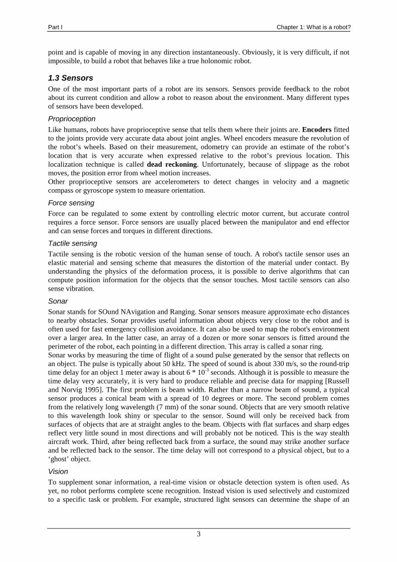
Sonar Sonar stands for SOund NAvigation and Ranging. Sonar sensors measure approximate echo distances to nearby obstacles. Sonar provides useful information about objects very close to the robot and is often used for fast emergency collision avoidance. It can also be used to map the robot's environment over a larger area. In the latter case, an array of a dozen or more sonar sensors is fitted around the perimeter of the robot, each pointing in a different direction. This array is called a sonar ring. Sonar works by measuring the time of flight of a sound pulse generated by the sensor that reflects on an object. The pulse is typically about 50 kHz. The speed of sound is about 330 m/s, so the round-trip time delay for an object 1 meter away is about 6 * 10-3 seconds. Although it is possible to measure the time delay very accurately, it is very hard to produce reliable and precise data for mapping [Russell and Norvig 1995]. The first problem is beam width. Rather than a narrow beam of sound, a typical sensor produces a conical beam with a spread of 10 degrees or more. The second problem comes from the relatively long wavelength (7 mm) of the sonar sound. Objects that are very smooth relative to this wavelength look shiny or specular to the sensor. Sound will only be received back from surfaces of objects that are at straight angles to the beam. Objects with flat surfaces and sharp edges reflect very little sound in most directions and will probably not be noticed. This is the way stealth aircraft work. Third, after being reflected back from a surface, the sound may strike another surface and be reflected back to the sensor. The time delay will not correspond to a physical object, but to a ‘ghost’ object.

Vision To supplement sonar information, a real-time vision or obstacle detection system is often used. As yet, no robot performs complete scene recognition. Instead vision is used selectively and customized to a specific task or problem. For example, structured light sensors can determine the shape of an

Part I Chapter 1: What is a robot?

4

object by projecting stripes of light on it and stereo cameras provide pairs of images recorded simultaneously for depth calculations. Computer vision requires knowledge of the field of computer graphics and image processing and will not be addressed in this report. For more on computer vision see [Ballard and Brown 1982].

Part I Chapter 2: Intelligence in robots

5

Chapter 2: Intelligence in robots Most Artificial intelligence researchers that study robotics are working on mobile robots. Mobile robots pose a unique challenge to the Artificial intelligence community, since they are inherently autonomous and force the researcher to deal with issues such as uncertainty in sensing and action, planning, learning, reliability, and real-time response. By improving and expanding the knowledge of how to successfully integrate these issues into one single system, fundamental contributions can be made to Artificial intelligence research.

2.1 The development of autonomous robots One of the first mobile robots, Shakey, was constructed in the late 1960s at the Stanford Research Institute [Nilsson 1969]. The robot used the STRIPS planning system, two independently controlled stepper motors and had a television camera and optical range finder mounted at the top. Shakey demonstrated that general-purpose planning systems were not very efficient and much to slow for practical use. Further research focused on faster processing and higher efficiency. In the mid 1980s many researchers began to question the ‘classical’ planning view of intelligent agent and robot design and started working on situated automata, finite-state-machines whose inputs are directly linked to the outputs (reflex agent). The robot Flakey that was based on the situated automata theory performed well and even won second place in the First American Association for Artificial Intelligence (AAAI) robot competition and exhibition held in San Jose in 1992. In 1986, Rodney Brooks published his paper [Brooks 1986] on the subsumption architecture, a robot control system based on finite-state-machines, which lead to the development of a new approach in robotics called behavior-based robotics.

2.2 Learning The goal of learning in a robot is to prepare it to deal with unforeseen situations and circumstances in its environment. The fact that even the simplest of animals seem to be adaptable suggests that learning must be important for survival in the animal world.

When is learning useful? There are two main benefits of learning in biological systems. First, learning lets the animal adapt to different circumstances in the world, giving it a wider range of environmental conditions in which it can operate effectively. Second, learning reduces the amount of genetic material and intermediate structures required for building the complete functioning adult animal. In some circumstances, it is simpler to build a small structure capable of constructing a larger one, than to specify the larger structure directly. The first aspect of learning in animals directly applies to robots as well. We would like our robots to adapt to changing external circumstances (e.g. changes in terrain), adapt to changing internal circumstances (e.g. drift in sensors and actuators, loss of power), and perform new tasks when appropriate. The second aspect does not transfer directly to robot control, unless they are programmed using genetic techniques. We can distinguish three types of knowledge that would be useful for a robot to acquire: 1. Hard to program knowledge: information that is very difficult to program by hand may be

obtained by showing examples or guiding the robot. 2. Unknown information: the information necessary to program the robot is simply not available.

For example, a map of the terrain the robot will be working in. 3. Changing environments: the world is a dynamic place. Even if we had a complete model of the

environment to begin with, this knowledge could quickly become obsolete in a dynamic environment. Also slower changes may occur, such as the calibration of the robot's own sensors and effector.

Part I Chapter 2: Intelligence in robots

6

To determine what types of information should be learned and what should be built-in, we must analyze the benefits and the costs of providing a robot with a learning capability. An important question is: “is the robot is better off for having the learning capability?” To answer this question one must take into account whether investing the same resources of research effort, runtime code size, and computing power into a directly engineered solution would have resulted in an equally successful and robust robot.

Learning approaches Much research effort has been devoted to tabula rasa or strong learning techniques that assume no built-in information. In this approach nothing is predefined and everything must be learned. Although in theory robots should be able to learn everything, in practice it is difficult for them to learn anything at all. Learning from scratch may be an interesting intellectual challenge, but many researchers feel that this poses an unreasonably difficult problem [Brooks 1990]. So far, strong learning approaches have led to only weak results, while weak learning approaches, where the robot has many built-in capabilities or much a priori knowledge, have been much more successful. However, the problem with weak learning is that the structure of the built-in knowledge restricts what the robot can learn. Reducing built-in structure eases the programming task and reduces the learning bias, but it also slows down the learning process. A compromise that combines the benefits of both is subsumable learning. With subsumable learning the robot is influenced to learn certain classes of behaviors by the nature of its existing knowledge. It uses the weak learning ability to adapt to its environment and has a more general strong learning component, capable of overriding the weaker system. Based on the type of information that is learned, we can divide robot learning approaches into four main categories:

1. Learning numerical functions for calibration or parameter adjustment. This type of learning optimizes operational parameters in an existing behavioral structure. In many cases the parameters of a robot can not be predicted. Due to sensor drift, environmental conditions, and unmodeled properties of the mechanical system, choosing or computing these values has to be done at run-time. Function learning is the weakest form of learning as the structure of the behavior-producing programs is predetermined and does not change based on experience. Rather than introducing new knowledge, it fine-tunes existing knowledge. Based on the number of successful performing robots, the function approximation approach has been most successful to date.

2. Learning about the world. This type of learning creates and alters some internal

representation of the world. The information usually is represented in some abstract symbolic form that is used for computing actions. Learning about the world can vary from learning maps of the environment to learning abstract concepts.

3. Learning to coordinate behaviors. This type of learning attempts to solve the action selection

problem, i.e. it tries to determine when particular actions or behaviors are to be executed. Reinforcement learning methods have been shown to be well-suited for this type of learning, since they produce precisely the kind of mapping between conditions and actions needed to decide how to behave at each distinct point in the state space.

4. Learning new behaviors. This type of learning builds new behavioral structures (as opposed

to the three previous ones). Reinforcement learning techniques have been used to learn new behaviors, but only in the sense that behaviors are constructed from arbitrary sequences of actions. An entirely different approach to learning behaviors that holds some promise, is the use of genetic programming. This type of learning has been tried in simulation [Koza 1990][Koza 1992] and has recently been used to create simple behaviors in real robots.

Part I Chapter 2: Intelligence in robots

7

2.3 Reinforcement learning Reinforcement learning has been applied to learn new behaviors and to coordinate existing ones. At the moment, it is probably the most popular way of learning in robots. Reinforcement learning systems attempt to learn a behavior by exploring all of the actions in all of the available states (trail-and-error) and rank them in the order of appropriateness. It uses rewards and/or punishments to alter numerical values in a controller. A component capable of evaluating the response is needed to send the necessary reinforcement signal to the control system. This component can be a human watching the robot or a software module programmed to evaluate the robot’s actions. The first is called supervised learning, the latter is unsupervised learning. The feedback to the control system provides information about the quality of the behavioral response. It may be as simple as a binary pass/fail or a more complex numeric evaluation. There is no specification as to what the correct response would be, only how well the particular response worked. The problem of learning an optimal strategy consists of searching for paths connecting the current state with the goal in the state space. The longer the distance between a state and the goal, the longer it takes to learn the strategy. Breaking the problem into modules effectively shortens the distance between the reinforcement signal and the individual actions, but this requires built-in domain information. One of the major problems of reinforcement learning is credit assignment. It is hard to determine which of the individual components is largely responsible for the success or failure of a response. Another important weakness of reinforcement learning is the ‘unstructured’ use of the input. Since no explicit domain information is used, the entire space of state-action pairs must be explored, but this space grows exponentially with the number of sensors. Also, reinforcement learning depends on the ability to detect in which state the robot is in to map it to the appropriate action. Sensor noise and errors increase state uncertainty, which slows down the learning process even further. In spite of its weaknesses, reinforcement learning appears to be a promising direction for learning with real robots, in particular because it uses direct information from the world to improve the robot's performance. Several reinforcement learning algorithms have been effectively used in robots: • With Q-learning actions and states are evaluated together. A single utility Q-function is learned

to evaluate both actions and states. Reward actions are propagated across states so that rewards from similar states aid the learning process. Different Q-learning forms use different ways to detect similar states. Q-learning currently dominates robotic reinforcement learning approaches.

• Adaptive Heuristic Critic (AHC) methods are methods in which a decision policy for action is learned independently from the utility cost function for state evaluation. AHC methods often are implemented in neural network systems.

• Statistical correlation is used to associate rewards with actions.

Applications Maes and Brooks [Maes and Brooks 1990] studied reinforcement learning with Genghis, a robot hexapod. They used a rule-based subsumption architecture for the robot controller which consists of thirteen high-level behaviors using two sensors for feedback. Two touch sensors were located on the bottom of the robot (fore and aft) to determine when the body of the robot hits the floor, and a trailing wheel was used to measure forward progress. Genghis’ task was to learn to move forward. Negative feedback was given when both of its touch sensors made contact with the ground and positive feedback was given when the trailing wheel indicated that the robot was moving forward. At IBM, Mahadevan and Connell [Mahadevan and Connell 1991] used Q-learning to teach a behavior-based robot how to push a box. The robot’s learning problem involved deciding which of the five possible actions would enable it to find and push boxes around a room efficiently without getting stuck. The robot’s performance was compared to its performance when controlled by a hand-programmed controller.

Part I Chapter 2: Intelligence in robots

8

2.4 Artificial neural networks

In the real world, it is difficult to learn with hand-programmed algorithms. The continuously changing environment and uncertainty caused by these changes requires a flexible learning system. Artificial neural networks provide this. Learning in neural networks occurs through the adjustment of synaptic weights by an error minimization procedure. The advantage of the use of neural networks is the fact that the system does not need to have specific properties for specific problems. The system tries to determine these properties itself. The only thing humans have to do is provide it with training examples and the corresponding action or reinforcement. Hebb developed one of the earliest training algorithms for neural networks [Hecht-Nielsen 1989]. Hebbian learning increases synaptic strength along the neural pathways associated with a stimulus and a correct response, strengthening frequently used paths. The most used neural network model is the feedforward, multilayer network with (different versions of) the backpropagation learning algorithm. Other models like Kohonen, Hopfield or Grossberg recently are increasing in popularity. For a more in-depth description of neural networks see [Aleksander and Morton 1995] or [Hecht-Nielsen 1989].

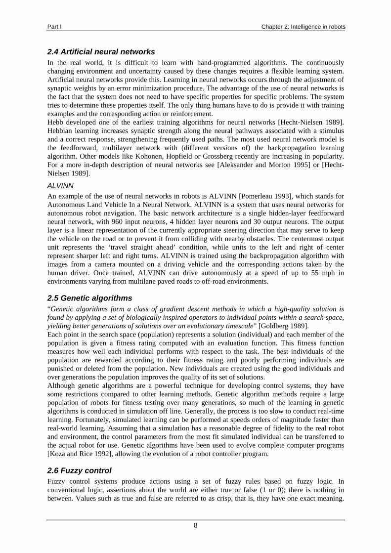
ALVINN An example of the use of neural networks in robots is ALVINN [Pomerleau 1993], which stands for Autonomous Land Vehicle In a Neural Network. ALVINN is a system that uses neural networks for autonomous robot navigation. The basic network architecture is a single hidden-layer feedforward neural network, with 960 input neurons, 4 hidden layer neurons and 30 output neurons. The output layer is a linear representation of the currently appropriate steering direction that may serve to keep the vehicle on the road or to prevent it from colliding with nearby obstacles. The centermost output unit represents the ‘travel straight ahead’ condition, while units to the left and right of center represent sharper left and right turns. ALVINN is trained using the backpropagation algorithm with images from a camera mounted on a driving vehicle and the corresponding actions taken by the human driver. Once trained, ALVINN can drive autonomously at a speed of up to 55 mph in environments varying from multilane paved roads to off-road environments.

2.5 Genetic algorithms “Genetic algorithms form a class of gradient descent methods in which a high-quality solution is found by applying a set of biologically inspired operators to individual points within a search space, yielding better generations of solutions over an evolutionary timescale” [Goldberg 1989]. Each point in the search space (population) represents a solution (individual) and each member of the population is given a fitness rating computed with an evaluation function. This fitness function measures how well each individual performs with respect to the task. The best individuals of the population are rewarded according to their fitness rating and poorly performing individuals are punished or deleted from the population. New individuals are created using the good individuals and over generations the population improves the quality of its set of solutions. Although genetic algorithms are a powerful technique for developing control systems, they have some restrictions compared to other learning methods. Genetic algorithm methods require a large population of robots for fitness testing over many generations, so much of the learning in genetic algorithms is conducted in simulation off line. Generally, the process is too slow to conduct real-time learning. Fortunately, simulated learning can be performed at speeds orders of magnitude faster than real-world learning. Assuming that a simulation has a reasonable degree of fidelity to the real robot and environment, the control parameters from the most fit simulated individual can be transferred to the actual robot for use. Genetic algorithms have been used to evolve complete computer programs [Koza and Rice 1992], allowing the evolution of a robot controller program.

2.6 Fuzzy control Fuzzy control systems produce actions using a set of fuzzy rules based on fuzzy logic. In conventional logic, assertions about the world are either true or false (1 or 0); there is nothing in between. Values such as true and false are referred to as crisp, that is, they have one exact meaning.

Part I Chapter 2: Intelligence in robots

9

Fuzzy logic allows variables to take on values between true and false, depending on how much they belong to a particular fuzzy set. In fuzzy logic these variables have linguistic names, for example fast, slow, far, big, etc. Membership functions measure the degree of similarity a variable has in its associated fuzzy set. A fuzzy logic control system consists of the following:

• Fuzzifier: maps a set of crisp sensor readings onto a collection of fuzzy input sets. • Fuzzy rule base: contains a collection of IF-THEN rules. • Fuzzy inference engine: maps fuzzy sets onto other fuzzy sets according to the rule base

and membership functions. • Defuzzifier: maps fuzzy output sets onto a set of crisp actuator commands.

Fuzzy systems are more flexible than conventional rule-based methods and allow more robust integration of sensor-motor commands than conventional production systems. Learning can also be used in fuzzy control systems and deals with learning the fuzzy rules of the rule base.

2.7 Other learning methods Our description of learning methods used with robots is by no means complete and many other powerful learning methods are just beginning to be explored for use in robotics. Some examples are mentioned briefly below. Case-based learning uses experiences are organized and stored as a case structure, then retrieved and adapted as needed based on the current situation. The basic algorithm is as follows:

1. Classify the current problem. 2. Use the resulting problem description to retrieve similar case(s) from case memory. 3. Adapt the old case’s solution to the new situation’s specifics. 4. Apply the new solution and evaluate the results. 5. Learn by storing the new case and its results.

Memory-based learning goes one step further than case-based learning. Many individual records of past experiences are used to derive function approximators for control laws. Complex control functions are approximated by interpolation of related past successful experiences. Explanation-based learning uses (symbolic) models of the domain to guide the generalization and specialization of a concept by induction. Learning occurs on an instance-by-instance basis, with refinement of the underlying model occurring at all steps in the process. Domain-specific knowledge is crucial for this process to operate effectively.

Part I Chapter 3: Mapping, localization and navigation

10

Chapter 3: Mapping, localization and navigation Navigation and mapping are crucial to all mobile robot systems. Navigation and mapping tasks include sonar sensor interpretation, collision avoidance, localization and path planning.

3.1 Mapping Mapping is the process of constructing a model of the environment based on sensor measurements. There are different approaches to representing and using spatial information. On one side, there are purely grid-based maps, also called geometric or metric maps. In these representations, the robot's environment is defined by a single, global coordinate system in which all mapping and navigation takes place. Typically, the map is a grid with each cell of the grid representing some amount of space in the real world. These approaches work well within bounded environments where the robot has opportunities to realign itself with the global coordinate system using external markers. On the other side are topological maps, also called qualitative maps, in which the robot's environment is represented as places and connections between places. This approach has the advantage that it eliminates the inevitable problems of dealing with movement uncertainty. Movement errors do not accumulate in topological maps as they do in maps with a global coordinate system since the robot only navigates locally, between places. Topological maps are also more compact in their representation of space because they only represent interesting places and not the entire environment. The disadvantage of this approach is that the robot has to be able to make the distinction between different places.

Creating and using grid-based maps Each grid cell of a grid-based map contains a value that indicates the presence or absence of an obstacle in the corresponding region of the environment. This value measures the robot's subjective belief whether or not its center can be moved to the center of that cell. There are several ways to construct grid-based maps, but the most popular methods use sonar sensors or stereo cameras. Sonar sensor readings can be translated into occupancy values for each grid cell. For example, a neural network with backpropagation can be used to map sonar measurements to occupancy values [Kortenkamp et al 1998]. The training examples are obtained by operating a robot in a known environment and recording and labeling its sensor readings. Once trained, the network generates values that can be interpreted as a probability for occupancy. Neural networks can easily be adapted to new circumstances (different walls reflect in different ways) and can process multiple sensor readings simultaneously. A second source of occupancy information can be gathered with a stereo camera system that provides pairs of images recorded simultaneously from different spatial viewpoints. Much like vision done by humans, stereo images can be used to compute depth information. Large unstructured obstacles such as walls are ‘invisible’ to a camera and will not be mapped, therefore stereo vision alone can not be sufficient for building accurate maps. On the other hand, stereo vision gives more accurate obstacle information than sonar sensors, due to the higher resolution of cameras. It frequently detects obstacles that are invisible to sonar sensors, such as objects that absorb sound. Maps built with sonar and stereo vision can be integrated by taking the maximum occupancy value at each grid cell.

Creating and using topological maps Topological maps represent robot environments by graphs. Nodes in these graphs correspond to distinct situations, places or landmarks. A link connects two nodes if a direct path exists between them. Topological maps are more compact than grid-based maps and thus allow faster planning. The construction of topological maps can be done with the use of grid-based maps in the following way [Kortenkamp et al 1998]:

Part I Chapter 3: Mapping, localization and navigation

11

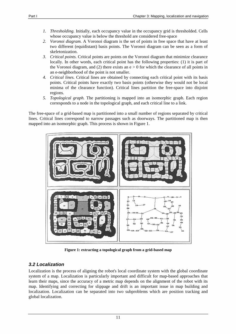
1. Thresholding. Initially, each occupancy value in the occupancy grid is thresholded. Cells whose occupancy value is below the threshold are considered free-space

2. Voronoi diagram. A Voronoi diagram is the set of points in free space that have at least two different (equidistant) basis points. The Voronoi diagram can be seen as a form of skeletonization.

3. Critical points. Critical points are points on the Voronoi diagram that minimize clearance locally. In other words, each critical point has the following properties: (1) it is part of the Voronoi diagram, and (2) there exists an e > 0 for which the clearance of all points in an e-neighborhood of the point is not smaller.

4. Critical lines. Critical lines are obtained by connecting each critical point with its basis points. Critical points have exactly two basis points (otherwise they would not be local minima of the clearance function). Critical lines partition the free-space into disjoint regions.

5. Topological graph. The partitioning is mapped into an isomorphic graph. Each region corresponds to a node in the topological graph, and each critical line to a link.

The free-space of a grid-based map is partitioned into a small number of regions separated by critical lines. Critical lines correspond to narrow passages such as doorways. The partitioned map is then mapped into an isomorphic graph. This process is shown in Figure 1.

Figure 1: extracting a topological graph from a grid-based map

3.2 Localization Localization is the process of aligning the robot's local coordinate system with the global coordinate system of a map. Localization is particularly important and difficult for map-based approaches that learn their maps, since the accuracy of a metric map depends on the alignment of the robot with its map. Identifying and correcting for slippage and drift is an important issue in map building and localization. Localization can be separated into two subproblems which are position tracking and global localization.

Part I Chapter 3: Mapping, localization and navigation

12

Position tracking or position estimation refers to the problem of estimating the location of the robot while it is moving. Drift and slippage reduces the precision of the robot position within its global map. Global localization is the problem of determining the position of the robot under global uncertainty. This problem arises, for example, when a robot uses a map that has been generated previously and when it is not informed about its initial location within the map. Localization can be done in several ways: • With dead reckoning wheel encoders measure the revolution of the robot's wheels. This provides

a fairly accurate estimate of the robot's location relative to its previous location, but small errors can accumulate to large displacements.

• Every sensor reading (sonar and/or vision) is converted into a ‘local’ map that is compared with the global map. This is called map matching. The more correlated the two maps are, the more likely is the corresponding location of the robot.

• Using robot maneuverability, the fact that a robot moves to a location makes it unlikely that this location is occupied. Assuming the global map is correct, it can be used to derive further probabilistic constraints on the robot's location.

• For correcting rotational errors in an indoor (office) environment the global wall orientation can be used. This approach rests on the restrictive assumption that walls are either parallel or orthogonal to each other.

• Landmarks are used in various approaches for mobile robot localization. Recently, mechanisms that enable a robot to select its own landmarks, based on sonar and camera input, are explored. Artificial neural networks have been trained to recognize landmarks by minimizing the average localization error.

3.3 Navigation A navigation system can usually be divided into two parts: a global planner and a reactive collision avoidance module. The global path planner generates minimum-cost paths to the goal(s) using a map. As a result, it provides intermediate goals to the collision avoidance routine that controls the velocity and the exact direction of motion of the robot.

Planning The idea of path planning is to let the robot always move on a minimum-cost path to the nearest goal. The global planner, in contrast with the collision avoidance routine, does not suffer from a local minimum problem, since it plans globally. With grid-based maps the minimum-cost path can be computed with algorithms like dynamic programming or A*. Topological planning is more efficient because of the compactness of topological maps. Topological planning is between three and four orders of magnitude more efficient than planning with grid-based maps. This is despite the fact that plans generated with topological maps are typically between one and four percent longer than plans generated using grid-based maps. A planner alone, however, is not sufficient to control the robot, because it does not take robot dynamics into account and because learned maps are incapable of capturing moving obstacles.

Collision avoidance The task of the collision avoidance routine (also called obstacle avoidance) is to navigate the robot to subgoals generated by the planner while avoiding collisions with obstacles. It adjusts the actual velocity of the robot and chooses the motion direction. For obvious reasons, the collision avoidance routine must operate in real-time. Depending on the speed and weight of the robot, it is very important that the robot’s dynamics (inertia and torque limits) are taken into account. The collision avoidance routine is easily trapped in local minima, such as U-shaped obstacle configurations. However, it reacts in real-time to unforeseen obstacles such as humans and is usually capable of changing the motion direction while the robot is moving.

Part I Chapter 4: Multi-robot systems

13

Chapter 4: Multi-robot systems Biology has shown that multi-agent societies, like schooling fish or insect colonies, offer significant advantages in the achievement of community tasks. For example, ants typically use chemical communication to convey information to one another. They lay down chemical trails via pheromones that increase efficiency and at the same time they avoid the need for explicit memory. Decision-making becomes a collective effort rather than a master-slave decision. Like ants, teams of robots have significant advantages over individual robots in terms of performance, sensing capabilities, and fault tolerance.

4.1 Tasks Coordinating activity is important for a society. The society needs to remain together and work on a common goal. Specialization can occur based upon the need of the society. Typical tasks for societies of robots include:

• Foraging: randomly placed items are distributed throughout the environment and the team’s task is to carry them back to a central location.

• Consuming: the robots perform work on the desired objects in place, rather than carrying them back to a home base. This may involve assembly or disassembly operations, for example clearing a minefield.

• Grazing: the robot team covers a certain area. The potential applications of this social behavior include lawn mowing, surveillance operations and vacuuming.

• Formation or flocking: the team of robots assumes a geometric pattern and maintains it while moving. This behavior can be useful for exploration.

• Object transport: requires a distribution of robots around the desired object with the goal being to move it to a particular location. This task can also be regarded as a subtask of foraging.

The behavioral architecture of the robots in a multi-robot system is only one of many design issues that have to be made during team design. Other aspects that need to be considered are the communication protocols between team members and the societal structure. To effectively evaluate societal system performance, specific metrics must be introduced. One useful metric is speedup, a measure of the performance of a team of N robots relative to N times the performance of a single robot.

4.2 Communication Communication plays a large role in coordinating teams of robots. Communication is not necessary for cooperation but it is often desirable. Range, content, and guarantees for communication are important factors in the design of social behavior. Communication is not free and can be undependable. It can be done explicitly, through direct channels, or indirectly, through the observation of other robot’s behaviors or changes in the environment. An example of the latter is trail marking. The major roles of communication in robot teams are:

• Synchronization of action: certain tasks require actions to be performed simultaneously or in

a particular sequence. • Information exchange: different robots have varying perspectives on the world based on their

spatial position or knowledge of past events and may need to communicate them. • Negotiations: decisions can be made regarding who should do what.

MacLennan has studied whether communication is important for cooperation [MacLennan 1991]. In his studies the societies in which communication evolved were 84% fitter than those in which

Part I Chapter 4: Multi-robot systems

14

communication was suppressed. Nonetheless, is has been has established that for certain classes of tasks, explicit communication is not a prerequisite for cooperation.

4.3 Social learning Various forms of machine learning have been applied to robotic teams, including reinforcement learning and imitation. Social learning is the process of acquiring new (cooperative) behavior patterns by learning from others. Social learning includes learning how to perform a behavior, and when to perform it. Mataric defines the basic forms of social learning as imitation or mimicry and social facilitation [Mataric 1994]. Imitation involves first observing another agent’s actions (either human or robot), then encoding that action in some internal representation and finally reproducing the initial action. Reinforcements can result from a robot’s action directly, from observation of another robot’s actions, or from observations of the reinforcement another robot receives Tensions between individual and group needs can exist. Robots may be strongly self-interested and have no concern for the society’s overall well being. Optimization in social robots usually focuses on minimizing interference between robots and maximizing the society’s reward.

4.4 Advantages and disadvantages To summarize, teaming robots together has both an upside and a downside. The positive aspects are:

• Improved system performance: if tasks are decomposable, the ‘divide and conquer’-strategy can be applied. The parallelism inherent in teaming causes tasks to be completed more efficient.

• Task enablement: the ability to do tasks that would be impossible for a single robot. • Distributed sensing: information sharing beyond the range of the sensors on an individual

robot. • Fault tolerance: robot redundancy and reduced individual complexity can increase overall

system reliability.

The negative aspects are:

• Interference: robots have physical size that can cause blockage or collisions. They may compete over things like food or information. Interference is also referred to as ‘resource competition’.

• Communication cost and robustness: communication is not free and requires additional hardware, computational processing, and energy. Communication can also suffer due to noisy channels, electronic countermeasures, and deceit by other robots.

• Uncertainty concerning other robots’ intentions: coordination generally requires knowing what the other robot is doing. When this is unclear because of lack of knowledge or poor communication, robots may compete rather than cooperate.

15

PART II: Behavior-based robotics

Part II Chapter 5: History of behavior-based robotics

16

Chapter 5: History of behavior-based robotics

5.1 Early developments In the late 1940s, Norbert Wiener lead the development of cybernetics which is a combination of control theory, information science and biology that seeks to explain the common principles of control and communication in both animals and machines. In 1953, W. Grey Walter applied these principles in the creation of a robotic design termed ‘Machina Speculatrix’, which was later transformed into hardware as Grey Walter’s tortoise. The tortoise consisted of two sensors, two actuators and two ‘nerve’ cells or vacuum tubes and it could demonstrate behaviors like seek light, head toward weak light, back away from bright light, turn, and recharge battery. Three decades after Walter, Valentine Braitenberg revived his behavior ideas [Braitenberg 1984]. Braitenberg’s vehicles used inhibitory and excitatory influences, directly coupling the sensors to the motors. Seemingly complex behavior resulted from relatively simple sensor-motor combinations. However, just like Walter’s tortoise, the Braitenberg vehicles were inflexible and could not be reprogrammed.

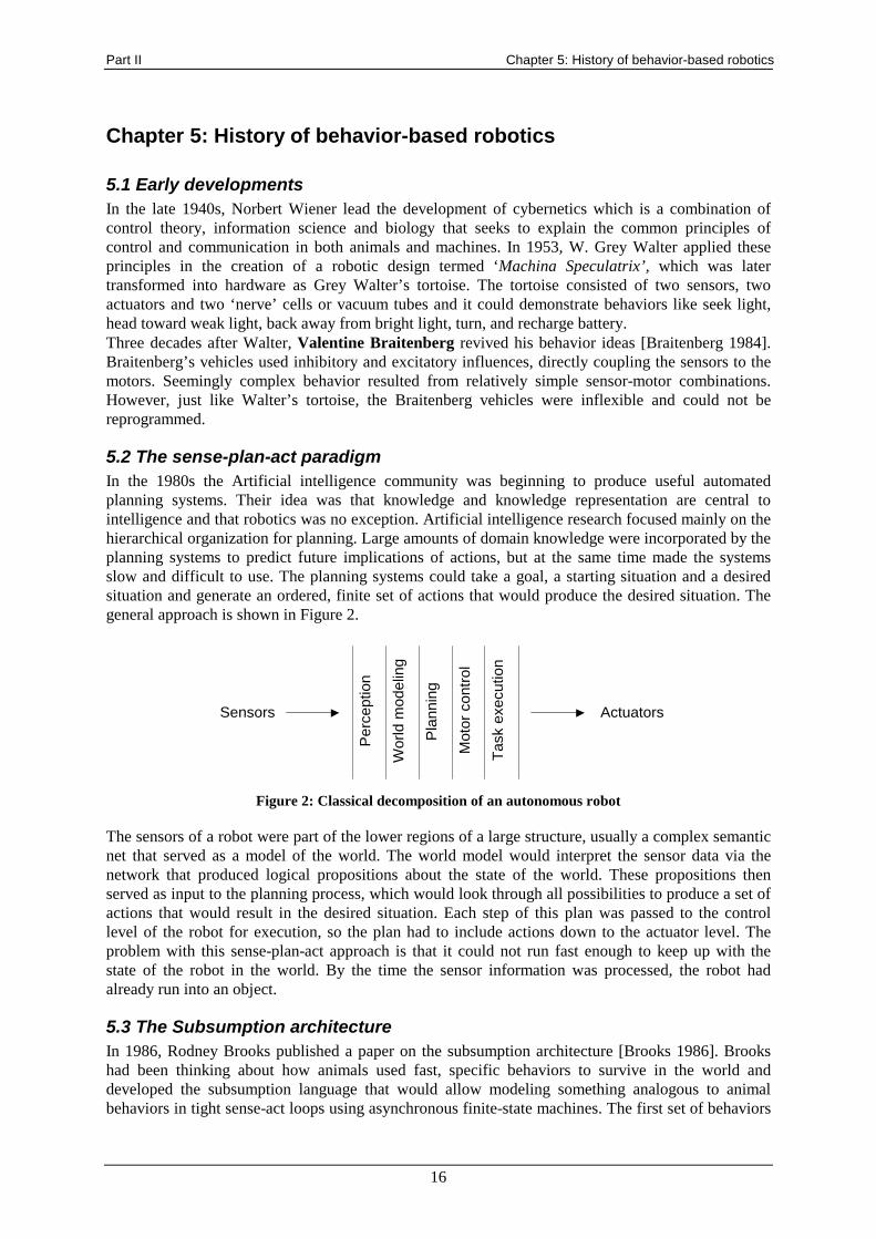
5.2 The sense-plan-act paradigm In the 1980s the Artificial intelligence community was beginning to produce useful automated planning systems. Their idea was that knowledge and knowledge representation are central to intelligence and that robotics was no exception. Artificial intelligence research focused mainly on the hierarchical organization for planning. Large amounts of domain knowledge were incorporated by the planning systems to predict future implications of actions, but at the same time made the systems slow and difficult to use. The planning systems could take a goal, a starting situation and a desired situation and generate an ordered, finite set of actions that would produce the desired situation. The general approach is shown in Figure 2.

Sensors

Per

cept

ion

Wor

ld m

odel

ing

Pla

nnin

g

Task

exe

cutio

n

Mot

or c

ontro

l

Actuators

Figure 2: Classical decomposition of an autonomous robot

The sensors of a robot were part of the lower regions of a large structure, usually a complex semantic net that served as a model of the world. The world model would interpret the sensor data via the network that produced logical propositions about the state of the world. These propositions then served as input to the planning process, which would look through all possibilities to produce a set of actions that would result in the desired situation. Each step of this plan was passed to the control level of the robot for execution, so the plan had to include actions down to the actuator level. The problem with this sense-plan-act approach is that it could not run fast enough to keep up with the state of the robot in the world. By the time the sensor information was processed, the robot had already run into an object.

5.3 The Subsumption architecture In 1986, Rodney Brooks published a paper on the subsumption architecture [Brooks 1986]. Brooks had been thinking about how animals used fast, specific behaviors to survive in the world and developed the subsumption language that would allow modeling something analogous to animal behaviors in tight sense-act loops using asynchronous finite-state machines. The first set of behaviors

Part II Chapter 5: History of behavior-based robotics

17

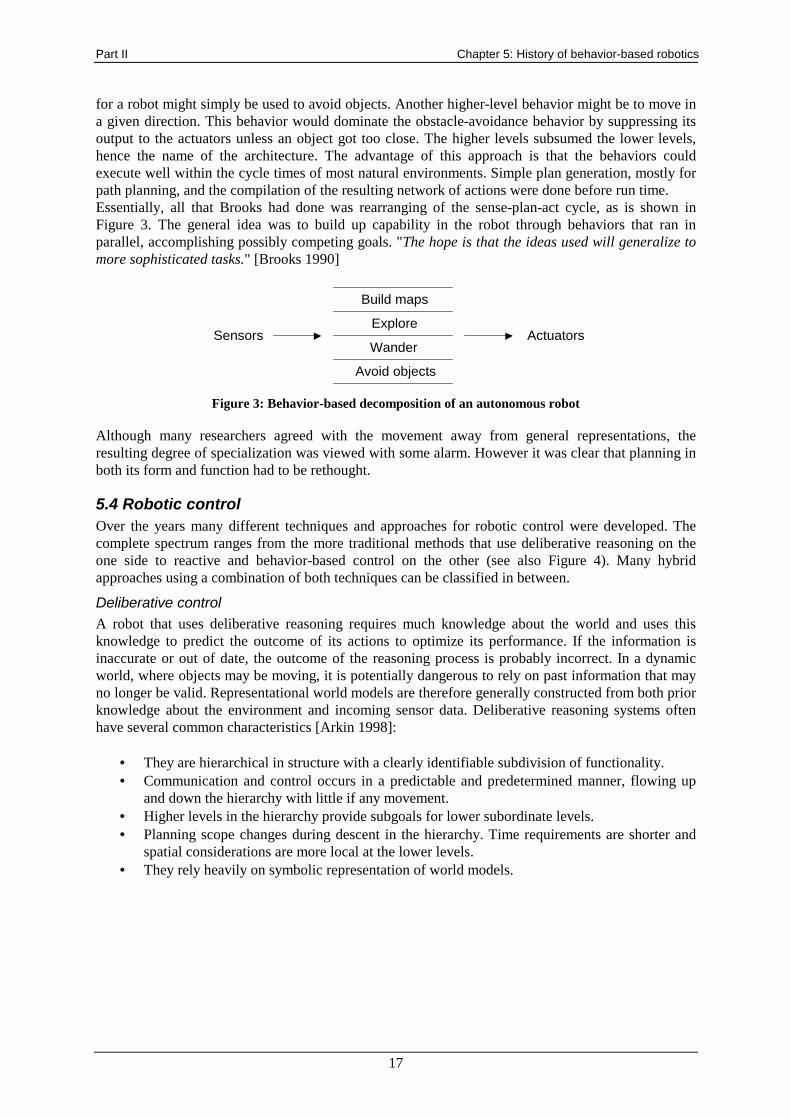
for a robot might simply be used to avoid objects. Another higher-level behavior might be to move in a given direction. This behavior would dominate the obstacle-avoidance behavior by suppressing its output to the actuators unless an object got too close. The higher levels subsumed the lower levels, hence the name of the architecture. The advantage of this approach is that the behaviors could execute well within the cycle times of most natural environments. Simple plan generation, mostly for path planning, and the compilation of the resulting network of actions were done before run time. Essentially, all that Brooks had done was rearranging of the sense-plan-act cycle, as is shown in Figure 3. The general idea was to build up capability in the robot through behaviors that ran in parallel, accomplishing possibly competing goals. "The hope is that the ideas used will generalize to more sophisticated tasks." [Brooks 1990]

SensorsExplore

Build maps

Avoid objects

WanderActuators

Figure 3: Behavior-based decomposition of an autonomous robot

Although many researchers agreed with the movement away from general representations, the resulting degree of specialization was viewed with some alarm. However it was clear that planning in both its form and function had to be rethought.

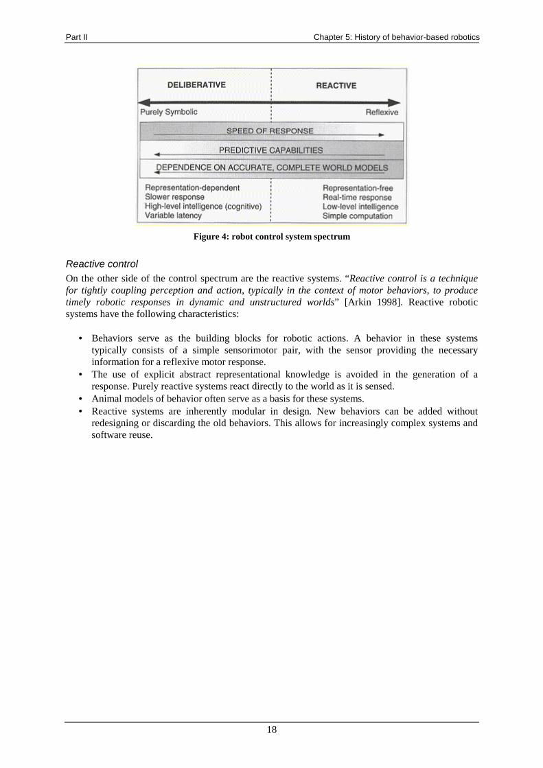
5.4 Robotic control Over the years many different techniques and approaches for robotic control were developed. The complete spectrum ranges from the more traditional methods that use deliberative reasoning on the one side to reactive and behavior-based control on the other (see also Figure 4). Many hybrid approaches using a combination of both techniques can be classified in between.

Deliberative control A robot that uses deliberative reasoning requires much knowledge about the world and uses this knowledge to predict the outcome of its actions to optimize its performance. If the information is inaccurate or out of date, the outcome of the reasoning process is probably incorrect. In a dynamic world, where objects may be moving, it is potentially dangerous to rely on past information that may no longer be valid. Representational world models are therefore generally constructed from both prior knowledge about the environment and incoming sensor data. Deliberative reasoning systems often have several common characteristics [Arkin 1998]:

• They are hierarchical in structure with a clearly identifiable subdivision of functionality. • Communication and control occurs in a predictable and predetermined manner, flowing up

and down the hierarchy with little if any movement. • Higher levels in the hierarchy provide subgoals for lower subordinate levels. • Planning scope changes during descent in the hierarchy. Time requirements are shorter and

spatial considerations are more local at the lower levels. • They rely heavily on symbolic representation of world models.

Part II Chapter 5: History of behavior-based robotics

18

Figure 4: robot control system spectrum

Reactive control On the other side of the control spectrum are the reactive systems. “Reactive control is a technique for tightly coupling perception and action, typically in the context of motor behaviors, to produce timely robotic responses in dynamic and unstructured worlds” [Arkin 1998]. Reactive robotic systems have the following characteristics:

• Behaviors serve as the building blocks for robotic actions. A behavior in these systems typically consists of a simple sensorimotor pair, with the sensor providing the necessary information for a reflexive motor response.

• The use of explicit abstract representational knowledge is avoided in the generation of a response. Purely reactive systems react directly to the world as it is sensed.

• Animal models of behavior often serve as a basis for these systems. • Reactive systems are inherently modular in design. New behaviors can be added without

redesigning or discarding the old behaviors. This allows for increasingly complex systems and software reuse.

Part II Chapter 6: Inspiration sources

19

Chapter 6: Inspiration sources Roboticists have struggled to provide their machines with capabilities that even simple animals possess: the ability to perceive and act within the environment in a meaningful and purposive manner. Behavior-based roboticists argue that there is much that can be gained for robotics through the study of neuroscience, psychology and ethology. Some scientists attempt to implement these results as closely as possible, testing the hypotheses of the biological models in question [Lund et al 1998]. Others use it as an inspiration to create more intelligent robots.

6.1 Neuroscientific and psychological basis for behavior At the cellular level of neurons, neuroscience has inspired computer scientists to create artificial neural networks, but also at the organizational level of brain structure much can be learned. Animal brains come in a very wide range of sizes. Simple invertebrates have nervous systems consisting of 103-104 neurons, whereas the brain of a small vertebrate such as a mouse contains approximately 107 neurons. The human brain has been estimated to contain 1010-1011 neurons. Despite a large variation in brain size, we can say several things in general about vertebrate brains. First, locality is a common feature. Brains are structurally organized into different regions each containing specialized functionality. Next, animals brains generally have three major subdivisions; the forebrain (containing the neocortex, limbic system, thalamus and hypothalamus), the brainstem (midbrain and hindbrain), and the spinal cord for control of various motor systems. Neuroscientific models have often had an impact on behavior-based robot design. Two examples are:

• The distinction between deliberative (willed) and automatic behavioral control systems. • Parallel mechanisms associated with both long- and short-term memory.

Psychological models focus on the concept of mind and behavior rather than on the brain itself. Various often opposing psychological schools have inspired roboticists. Examples are:

• Using stimulus-response mechanisms for the expression of behaviors. • Capturing the relationship a robot has with its environment based on theories of ecological

psychology. • Using computational models from cognitive psychology to describe a robot’s behavior within

the world.

6.2 Ethological basis for behavior Ethology is the study of animal behavior in its natural environment. For the true ethologist, the behavior of an organism is intimately coupled with its environment, so removing the animal from its environment destroys the context for its behavior. Animal behavior can be roughly categorized into three major classes:

1. Reflexes are rapid automatic and involuntary responses triggered by certain environmental stimuli. The reflexive response persists only as long as the duration of the stimulus. Further, the response intensity correlates with the stimulus’s strength. Certain escape behaviors, such as those found in snails and bristle worms, involve reflexive action.

2. Taxes are voluntary behavioral responses that direct the animal toward or away from a stimulus (attractive or aversive). Taxes occur in response to visual, chemical, mechanical and electromagnetic phenomena in a wide range of animals. Chemotaxis for example, can be seen in response to chemical stimuli, used in the trail following of ants.

3. Fixed-action patterns are time-extended response patterns triggered by a stimulus but persisting for longer than the stimulus itself. The strength and duration of the stimulus do not control the intensity and duration of the response. Unlike reflexes, fixed-action patterns may be

Part II Chapter 6: Inspiration sources

20

motivated and they may result from a much broader range of stimuli. Examples include egg-retrieving behavior of the greyling goose and the song of crickets.

One of the most important concepts for behavior-based robotics drawn from the field of ethology is the ecological niche. As defined by [McFarland 1981, page 411] “The status of an animal in its community, in terms of its relation to food and enemies, is generally called its niche”. Animals survive in nature because they have found a reasonably stable niche. They have a place where they can coexist with their environment. Evolution has shaped animals to fit their niche. As the environment is always changing, a successful animal must be capable of adapting to these changes or it will become extinct. Comparing the niche concept to robots, if a roboticist wants to build a system that is autonomous and can successfully compete with other environmental inhabitants, that system must find a stable niche or it (as an application) will be unsuccessful. Often economic pressures are sufficient to prevent the fielding of a robotic system. If humans are willing to perform the same task as a robot at a lower cost and/or with greater reliability then the robot will be unable to displace the human worker from the niche he already occupies. Thus, for a roboticist to design an effective real world system, the system must be targeted towards some niche. This is the reason that most robot applications are highly specialized, targeting a specific niche.

Part II Chapter 7: Designing robot behavior

21

Chapter 7: Designing robot behavior The behaviorist school of psychology teaches us that a behavior is a reaction to a stimulus. Transforming this idea to robotics, a robotic behavior generates a motor response reacting on a given stimulus from its sensors.

7.1 Design approaches A variety of approaches for behavior choice and design exist. Three different design paradigms for building behavior-based systems can be distinguished. As discussed in the previous chapter, biological models are often used as the basis for behavioral selection, design and validation. This called ethologically guided or ethologically constrained design. Another design approach is called situated activity. With situated activity behaviors are created that fit specific circumstances or situations in which the robots needs to respond. As soon as the robot finds itself in a new situation, it selects a new and more appropriate action. The third design approach is experimentally driven design that uses a bottom-up design strategy based on the need for additional functionality as the system is being built. The robot is equipped with a limited set of capabilities, experiments are run to see what works and what does not, and imperfect behaviors are debugged. New behaviors are added iteratively until the overall system performs satisfactory. Whatever the design basis, a generic classification of robot behaviors can be used to categorize the different ways in which a robotic agent can interact with its world. These behaviors are:

• Exploration / directional behaviors (move in a general direction) • Goal-oriented appetitive behaviors (move towards an attractor) • Aversive / protective behaviors (prevent collisions) • Path following behaviors (move on a designated path) • Postural behaviors (balance and stability) • Social / cooperative behaviors (multi-agent cooperation) • Teleautonomous behaviors (coordinate with human operator) • Manipulator-specific behaviors (arm-hand control)

Design choices for all robotic architectures involve issues such as whether to use analysis or synthesis, take a top-down or bottom-up design approach, and design for specific or general domains.

7.2 Behavioral encoding To encode the behavioral response that a stimulus should evoke, a functional mapping from the stimulus domain to the motor domain is needed. The robot’s motor response can be separated into two orthogonal components, strength and orientation. Strength indicates the magnitude of the response and orientation denotes the direction of action for the response. Behaviors can be represented as triples (S, R, β), with S being the domain of all interpretable stimuli, R the range of possible response, and β the behavioral mapping between S and R. Each individual stimulus s ∈ S is represented as a tuple (p, λ) where p is a particular type or perceptual class and λ the strength of the stimulus. The strength can be either discrete or continuous. The presence of a stimulus is necessary but not sufficient to evoke a motor response in a behavior-based robot. Only when the stimulus exceeds some threshold value t will it produce a response. A strength multiplier gi, or gain value associated with a particular behavior β can be used to turn off behaviors or increase the relative strength of the response. In formula this is represented as:

β: (p, λ) → {for all λ do: if λ < t then r = 0 /* no response */ else r = g * arbitrary function} /* response */

Part II Chapter 7: Designing robot behavior

22

Responses are coded in two forms, discrete encoding with an enumerable set of responses or continuous functional encoding with an infinite space of responses possible for a behavior. Rule-based methods (IF-THEN-rules) are often used for discrete encoding strategies. Approaches based on the potential-fields method are often used for the continuous functional encoding of robotic response.

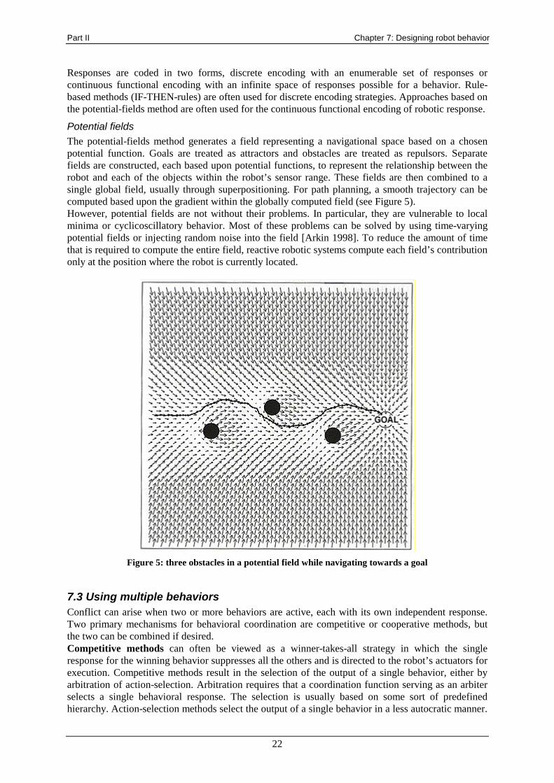
Potential fields The potential-fields method generates a field representing a navigational space based on a chosen potential function. Goals are treated as attractors and obstacles are treated as repulsors. Separate fields are constructed, each based upon potential functions, to represent the relationship between the robot and each of the objects within the robot’s sensor range. These fields are then combined to a single global field, usually through superpositioning. For path planning, a smooth trajectory can be computed based upon the gradient within the globally computed field (see Figure 5). However, potential fields are not without their problems. In particular, they are vulnerable to local minima or cyclicoscillatory behavior. Most of these problems can be solved by using time-varying potential fields or injecting random noise into the field [Arkin 1998]. To reduce the amount of time that is required to compute the entire field, reactive robotic systems compute each field’s contribution only at the position where the robot is currently located.

Figure 5: three obstacles in a potential field while navigating towards a goal

7.3 Using multiple behaviors Conflict can arise when two or more behaviors are active, each with its own independent response. Two primary mechanisms for behavioral coordination are competitive or cooperative methods, but the two can be combined if desired. Competitive methods can often be viewed as a winner-takes-all strategy in which the single response for the winning behavior suppresses all the others and is directed to the robot’s actuators for execution. Competitive methods result in the selection of the output of a single behavior, either by arbitration of action-selection. Arbitration requires that a coordination function serving as an arbiter selects a single behavioral response. The selection is usually based on some sort of predefined hierarchy. Action-selection methods select the output of a single behavior in a less autocratic manner.

Part II Chapter 7: Designing robot behavior

23

Here the behaviors actively compete with each other through the use of activation levels driven by both the robot’s goals and incoming sensor information. The behavior with the highest activation level wins. Cooperative methods offer an alternative to competitive methods by using behavioral fusion. This provides the ability to use the output of more than one behavior at a time. The central issue in combining the outputs of behaviors is finding a representation that allows fusion. One such representation is the previously discussed potential-fields. The most straightforward method here is the use of vector addition or superpositioning.

Behavioral assemblages Behavioral assemblages are the packages from which behavior-based robotic systems are constructed. An assemblage is recursively defined as an aggregation of behaviors or other assemblages. They serve as important abstractions that can be used to create higher-level behaviors from simpler ones. Each individual assemblage consists of a coordination operator and a number of behavioral components.

Emergent behavior Emergence is the appearance of novel properties in a system. Often emergence is viewed in an almost mystical sense regarding the capabilities of behavior-based systems. It is true that what occurs in a behavior-based system is often a surprise to the system’s designer, but this surprise does not come because of a shortcoming in the analysis of the behavioral building blocks and their coordination. Coordination functions are algorithms and hence are straightforward and contain no surprises. However, we cannot predict robot behavior exactly because the real world is filled with uncertainty and dynamic elements. The world cannot be faithfully modeled and is full of surprises. As Rodney Brooks [Brooks 1990] said it “…the world is its own best model. It is always exactly up to date. It always contains every detail there is to be known. The trick is to sense it appropriately and often enough.”

Part II Chapter 8: Behavior-based architectures

24

Chapter 8: Behavior-based architectures A common theme across robot systems is architecture. An architecture is a description of how a system is constructed from basic components and how those components fit together. Every robot has an architecture, even if implicitly.

8.1 Common features and differences Behavior-based robotic systems work best when the real world cannot be accurately characterized or modeled. Whenever engineering can remove uncertainty from the environment, purely behavior-based systems may not necessarily be the best solution for the task. Often this is not the case and behavior-based robotic architectures were developed in response to this difficulty. A wide range of architectural solutions exists under the behavior-based paradigm. Common features of behavior-based architectures are:

• An aversion to the use of representational knowledge. • A tight coupling between sensing and action. • Decomposition into meaningful units (behaviors or situation-action pairs).

The differences between behavior-based architectures are: • Choice of behaviors. • Used coordination methods (competitive or cooperative). • Response encoding method (discrete or continuous). • Programming methods. • Basis for development (ethological, situated activity or experimental).

Behavior-based architectures can be evaluated in terms of their support for parallelism, hardware retargetability, ecological niche fitting, modularity support, robustness, flexibility, ease of development, and performance. However, there is no accepted theory of architecture design that can be used to prove that one design is better than over another design.

8.2 Subsumption architecture In the mid-1980s, Rodney Brooks developed the subsumption architecture. Brooks argued that the sense-plan-act paradigm the Artificial intelligence community was using (see also paragraph 5.2 The sense-plan-act paradigm) led robotics researchers in the wrong direction. He further argued that complex behavior does not necessarily need a complex control system. The subsumption architecture is a layered architecture that uses arbitration strategies and augmented finite state machines as its basis. Task-achieving behaviors in the subsumption architecture are represented as separate layers with individual layers working on individual goals concurrently. At the lowest level, each behavior is represented with an augmented finite state machine (AFSM) model. Sensor inputs are directed to behaviors that need them. The lower levels have no awareness of higher levels. Higher levels can be added on an already working control system without further modifications to the lower levels. Complex actions subsume simpler behaviors, hence the name. Coordination in the subsumption architecture is done either by inhibition or suppression of signals. The subsumption architecture has been implemented on many robotic systems using rule-based encodings and an experimental design methodology. Some heuristics for the design and development of behaviors are [Mataric 1992]:

1. Specify the desired behavior(s) in qualitative terms. The behaviors are the goals of the system.

2. Specify the behavior in terms of the actions in the observer space. This is the process of breaking down the behavior into observable, disjoint actions that will serve as subgoals.

3. Specify the actions in terms of the robot’s effectors. This is the process of selecting the action set and the point at which the decision about the granularity of control is made.

Part II Chapter 8: Behavior-based architectures

25

8.3 Motor schemas The motor schemas approach, motivated by the biological sciences, appeared a few years after the subsumption architecture. Motor schemas are a software-oriented dynamic reactive architecture that is non-layered and cooperative [Arkin 1998]. Vectors serve as the continuous response-encoding mechanism with summation as the coordination strategy. Each motor schema has an output, an action vector that defines the way it should respond to the perceived stimuli, and all vectors are multiplied by its gain value and summed. No predefined hierarchy exists for coordination. Instead, the behaviors are configured at run-time. Perception is often conducted on a need-to-know basis. Individual perceptual algorithms provide the information that is necessary for a behavior to react. This is called action-oriented perception. Arkin has made a list for building a schema-based robotic system, which is as follows:

1. Characterize the problem domain in terms of the motor behaviors necessary to accomplish the task.

2. Decompose the motor behaviors to their most primitive level using biological studies, whenever feasible, for guidelines.

3. Develop formulas to express the robot’s reaction to perceived environmental events. 4. Conduct simple simulation studies assessing the desired behaviors’ approximate performance

in the proposed environment. 5. Determine the perceptual requirements needed to satisfy the inputs for each motor schema. 6. Design specific perceptual algorithms that extract the required data for each behavior, utilizing

action-oriented perception, expectations and focus-of-attention techniques to ensure computational efficiency.

7. Integrate the resulting control system onto the target robot. 8. Test and evaluate the system’s performance. 9. Iterate and expand behavioral repertoire as necessary.

8.4 Other architectures A wide range of other behavior-based architectures exists. Each approach is characterized by its choice of coordination mechanisms, the used response-encoding methods, the used behaviors, and the design methodology. Well-known architectures are:

• The circuit architecture that uses logical expressions for behavioral encoding, and abstraction coupled with arbitration.

• The action-selection architecture, which is a dynamic competition system with a high emergent quality using arbitration, developed by Pattie Maes.

• The colony architecture is a simplified version of subsumption, more straightforward in its implementation. It only uses suppression and is more flexible in behavioral relations.

• The animate agent architecture uses reactive action packages (RAPs), which are specific methods for certain tasks or situations.

Although behavior-based methods work excellent in dynamic environments, many roboticists would like to use representational knowledge in their robots. Research has been done on how to integrate various forms of representational knowledge into behavioral architectures. This will be the subject of the next chapter.

Part II Chapter 9: Knowledge representations

26

Chapter 9: Knowledge representations A controversy exists regarding the role of knowledge in robotic systems. Behavioral roboticists generally view the use of symbolic representational knowledge as an obstacle to efficient and effective robotic control. Others argue that strong forms of representational knowledge are needed to have a robot perform at anything above the level of a lower life form.

9.1 What is knowledge? Knowledge, much like intelligence, is a word that is very difficult to define. Information arises from data and knowledge can be said to emerge from information. Knowledge involves using information intelligently. Two important characteristics of knowledge include its predictive power and the need for the stored information to correlate with the environment. The more predictable the world, the more useful knowledge representations are since the predictive power of the knowledge will be higher. Knowledge can be characterized into three primary forms:

1. Explicit knowledge is symbolic discrete and manipulable knowledge, typically used as knowledge representations in traditional Artificial intelligence reasoning.

2. Implicit knowledge is non-explicit but reconstructable and can be made explicit through procedural usage.

3. Tacit knowledge is knowledge embedded in a system that existing processes cannot reconstruct.

Symbolic systems use explicit knowledge as defined above, subsymbolic systems (e.g. artificial neural networks) use either implicit or tacit knowledge. Knowledge can also be characterized by its durability. Transitory knowledge, which is derived from sensor data, corresponds to cognitive short-term memory. Persistent knowledge, which may originate from either a priori knowledge or sensor data, corresponds to long-term memory.

9.2 Knowledge in behavior-based systems Many roboticists, especially the ones using behavior-based systems, resist the use of explicit knowledge because of the symbol-grounding problem. The symbol-grounding problem refers to the difficulty in connecting the meaning (semantics) of an arbitrary symbol to a real world entity or event. It is easy to create a symbol that represents something, but it is difficult to attach the full meaning and implications of that real world object or event to the symbol. Often, other symbols are used to define the symbol that one is trying to describe. Although it appears contradictory, knowledge representations have been used in the control system of behavior-based robotic systems. We can distinguish two different types. Short-term memory (STM) uses representational knowledge for specific behaviors on a need-to-know basis, in a manner similar to action-oriented perception. As an analogy, this is called action-oriented knowledge representation. Long-term memory (LTM) can be divided in two forms: sensor-derived cognitive maps and a priori derived maps. In the first case information is directly received from the environment and gathered only during the lifetime of the robot in a particular environment. It is used to construct a stand-alone world model that is continuously updated to maintain a close correlation with the actual world. In the second case, information was gathered earlier and possibly independent of the robotic agent. A priori derived maps make it possible for a robot to navigate through an environment it has never visited before.

Short-term behavioral memory Behavioral memory provides certain advantages to a robot. It reduces the need for frequent sensor sampling in reasonably stable environments and it provides recent information to guide the robot to places outside its sensor range. Short-term memory is often used in single behaviors, usually obstacle avoidance. The memory serves as a buffer and translator for a limited number of previous sensings. It

Part II Chapter 9: Knowledge representations

27

is used while the robot is in the environment, discarded afterwards and must be reconstructed if the robot re-enters the environment. Although this might appear to penalize the robot by making it somewhat absentminded, it is actually valuable as it eliminates much of the difficulty of long-term localization (position relative to a map). Also, it is useful in dynamic environments where the position of obstacles may change over time.

Long-term memory maps Long-term memory representations can be used for mapping and navigational purposes. Map representational knowledge is usually encoded in either metric form (absolute measurements) or qualitative form (topological). One should note that the use of any form of map knowledge could be dangerous because the world may have changed since the map was constructed. Also, localization needs to be conducted for the robot to plan routes using its current position on the map. Sensor derived maps provide information directly obtained from the robot’s experiences in the world. As the world is sampled from the robot’s point of view, it is often better to use qualitative representations instead of metric ones because of the always-present inaccuracies in robot motion and sensor readings. The drawback of these navigational techniques is that the robot must have the ability to distinguish the different places in its environment.

9.3 Hybrid deliberative-reactive architectures Both deliberative planning systems and purely reactive control systems have their limitations, but using both forms of knowledge in a robotic architecture can make behavior-based navigation more flexible and general. Hybrid deliberative-reactive robotic architecture can combine the traditional abstract representational knowledge with the responsiveness, robustness, and flexibility of purely reactive systems. However, building such a hybrid system requires certain compromises. The interface between deliberation and reactivity is not yet well understood and a research in this area is still ongoing. An important design issue of hybrid control systems is the number of layers. Usually the hybrid architecture consists of two or three layers. In the case of two layers the interface between the layers is very important because it links rapid reactions with long-range planning. In the case of three layers the middle layer coordinates between the other two layers, much like the interface in the two-layer architecture. There are four main interface strategies for the various hybrid architectural designs:

1. Selection: planning is viewed as configuration and determines the behavioral composition and parameters used during execution.

2. Advising: the planner suggests changes that the reactive control system may or may not use. 3. Adaptation: the planner continuously alters the ongoing reactive behaviors based on the

changing conditions within the world and task requirements. 4. Postponing: planning is viewed as a least commitment process. The planner postpones making

decisions on action until as late as possible. Strong evidence exists that hybrid deliberative and behavior-based systems are found in biology, so research in this area could lead to new insights. For example, there seem to be two distinct systems concerned with controlling human behavior, a reactive and automatic system (e.g. when one’s hand touches something hot) and a willed and conscious control system (e.g. grasping something).

28

PART III: Evolutionary robotics

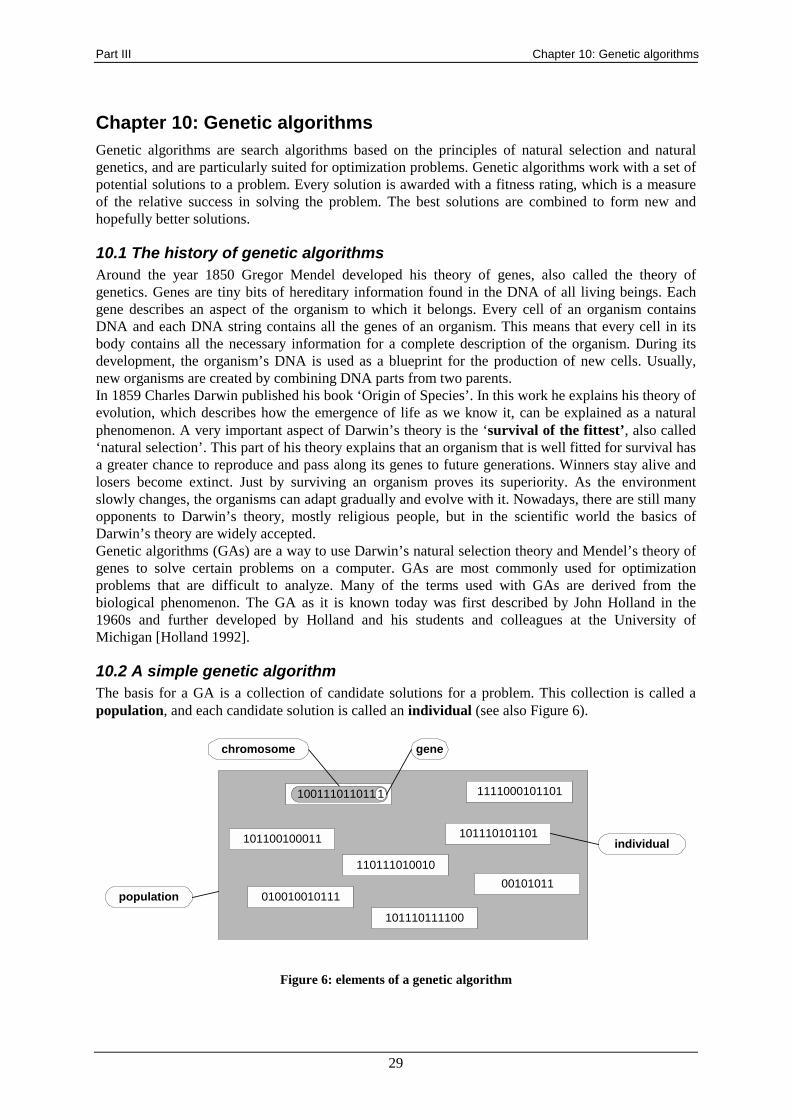
Part III Chapter 10: Genetic algorithms

29

Chapter 10: Genetic algorithms Genetic algorithms are search algorithms based on the principles of natural selection and natural genetics, and are particularly suited for optimization problems. Genetic algorithms work with a set of potential solutions to a problem. Every solution is awarded with a fitness rating, which is a measure of the relative success in solving the problem. The best solutions are combined to form new and hopefully better solutions.

10.1 The history of genetic algorithms Around the year 1850 Gregor Mendel developed his theory of genes, also called the theory of genetics. Genes are tiny bits of hereditary information found in the DNA of all living beings. Each gene describes an aspect of the organism to which it belongs. Every cell of an organism contains DNA and each DNA string contains all the genes of an organism. This means that every cell in its body contains all the necessary information for a complete description of the organism. During its development, the organism’s DNA is used as a blueprint for the production of new cells. Usually, new organisms are created by combining DNA parts from two parents. In 1859 Charles Darwin published his book ‘Origin of Species’. In this work he explains his theory of evolution, which describes how the emergence of life as we know it, can be explained as a natural phenomenon. A very important aspect of Darwin’s theory is the ‘survival of the fittest’, also called ‘natural selection’. This part of his theory explains that an organism that is well fitted for survival has a greater chance to reproduce and pass along its genes to future generations. Winners stay alive and losers become extinct. Just by surviving an organism proves its superiority. As the environment slowly changes, the organisms can adapt gradually and evolve with it. Nowadays, there are still many opponents to Darwin’s theory, mostly religious people, but in the scientific world the basics of Darwin’s theory are widely accepted. Genetic algorithms (GAs) are a way to use Darwin’s natural selection theory and Mendel’s theory of genes to solve certain problems on a computer. GAs are most commonly used for optimization problems that are difficult to analyze. Many of the terms used with GAs are derived from the biological phenomenon. The GA as it is known today was first described by John Holland in the 1960s and further developed by Holland and his students and colleagues at the University of Michigan [Holland 1992].

10.2 A simple genetic algorithm The basis for a GA is a collection of candidate solutions for a problem. This collection is called a population, and each candidate solution is called an individual (see also Figure 6).

101100100011

110111010010

010010010111

101110111100

00101011

1111000101101

101110101101

chromosome gene

10011101101111

population

individual

Figure 6: elements of a genetic algorithm

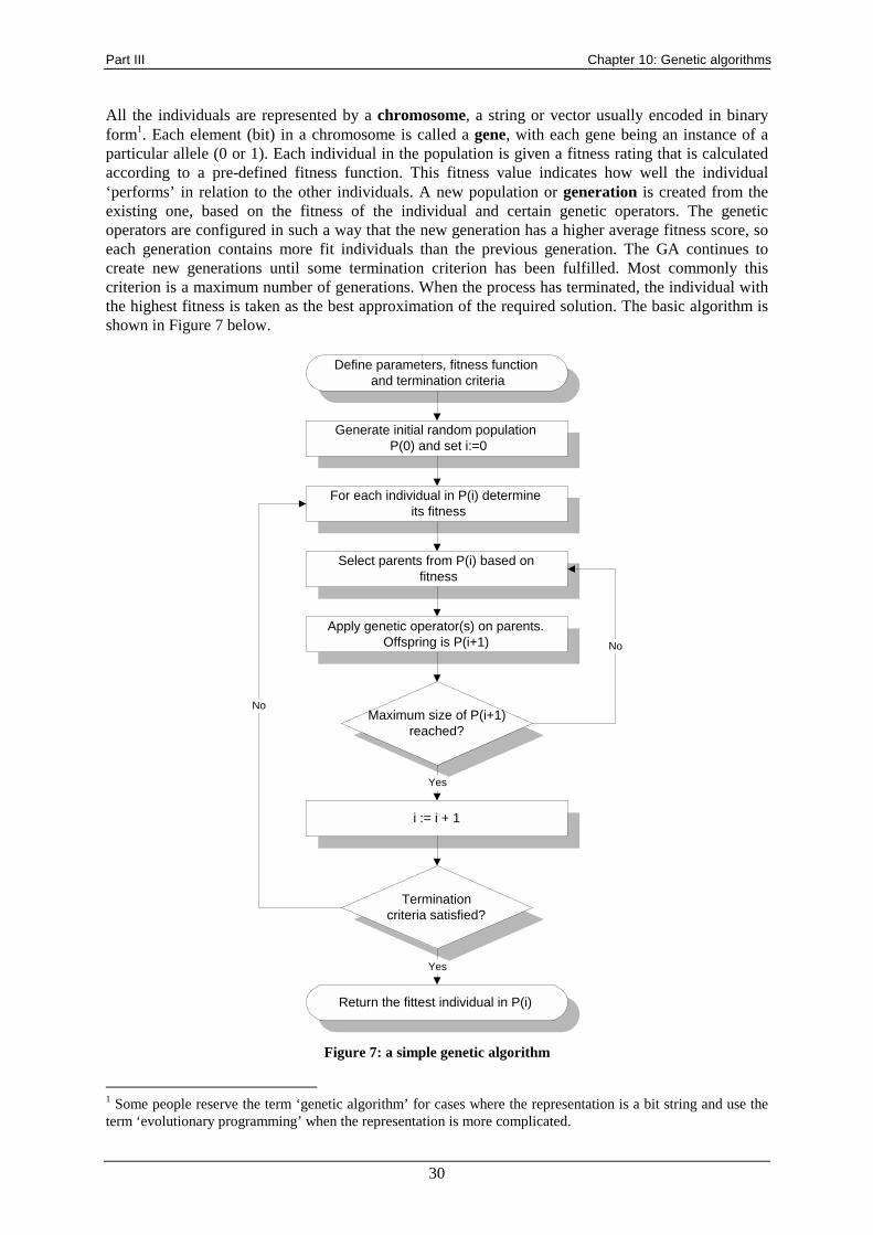
Part III Chapter 10: Genetic algorithms

30

All the individuals are represented by a chromosome, a string or vector usually encoded in binary form1. Each element (bit) in a chromosome is called a gene, with each gene being an instance of a particular allele (0 or 1). Each individual in the population is given a fitness rating that is calculated according to a pre-defined fitness function. This fitness value indicates how well the individual ‘performs’ in relation to the other individuals. A new population or generation is created from the existing one, based on the fitness of the individual and certain genetic operators. The genetic operators are configured in such a way that the new generation has a higher average fitness score, so each generation contains more fit individuals than the previous generation. The GA continues to create new generations until some termination criterion has been fulfilled. Most commonly this criterion is a maximum number of generations. When the process has terminated, the individual with the highest fitness is taken as the best approximation of the required solution. The basic algorithm is shown in Figure 7 below.

Generate initial random population P(0) and set i:=0

For each individual in P(i) determine its fitness

Select parents from P(i) based on fitness

Apply genetic operator(s) on parents.Offspring is P(i+1)

Maximum size of P(i+1)reached?

No

Yes

Terminationcriteria satisfied?

Return the fittest individual in P(i)

No

Yes

Define parameters, fitness function and termination criteria

i := i + 1

Figure 7: a simple genetic algorithm

1 Some people reserve the term ‘genetic algorithm’ for cases where the representation is a bit string and use the term ‘evolutionary programming’ when the representation is more complicated.

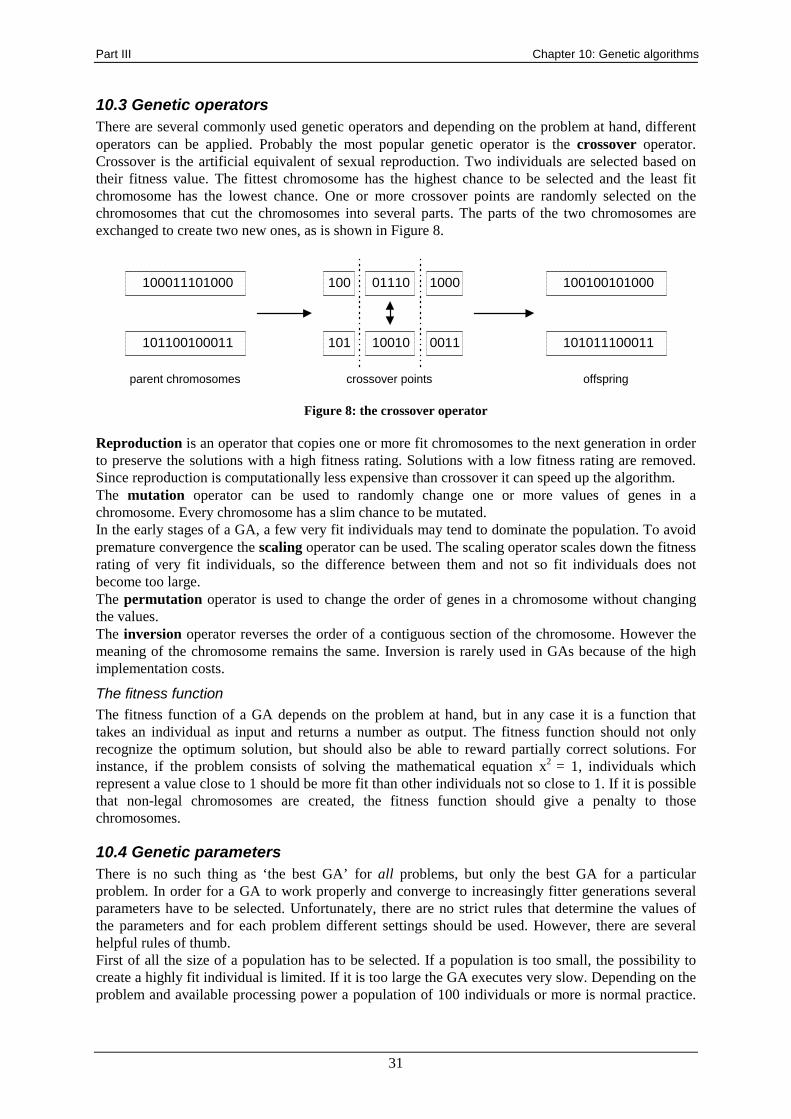
Part III Chapter 10: Genetic algorithms

31

10.3 Genetic operators There are several commonly used genetic operators and depending on the problem at hand, different operators can be applied. Probably the most popular genetic operator is the crossover operator. Crossover is the artificial equivalent of sexual reproduction. Two individuals are selected based on their fitness value. The fittest chromosome has the highest chance to be selected and the least fit chromosome has the lowest chance. One or more crossover points are randomly selected on the chromosomes that cut the chromosomes into several parts. The parts of the two chromosomes are exchanged to create two new ones, as is shown in Figure 8.

101100100011

100011101000

parent chromosomes

100 01110 1000

101 10010 0011

crossover points

100100101000

101011100011

offspring

Figure 8: the crossover operator

Reproduction is an operator that copies one or more fit chromosomes to the next generation in order to preserve the solutions with a high fitness rating. Solutions with a low fitness rating are removed. Since reproduction is computationally less expensive than crossover it can speed up the algorithm. The mutation operator can be used to randomly change one or more values of genes in a chromosome. Every chromosome has a slim chance to be mutated. In the early stages of a GA, a few very fit individuals may tend to dominate the population. To avoid premature convergence the scaling operator can be used. The scaling operator scales down the fitness rating of very fit individuals, so the difference between them and not so fit individuals does not become too large. The permutation operator is used to change the order of genes in a chromosome without changing the values. The inversion operator reverses the order of a contiguous section of the chromosome. However the meaning of the chromosome remains the same. Inversion is rarely used in GAs because of the high implementation costs.

The fitness function The fitness function of a GA depends on the problem at hand, but in any case it is a function that takes an individual as input and returns a number as output. The fitness function should not only recognize the optimum solution, but should also be able to reward partially correct solutions. For instance, if the problem consists of solving the mathematical equation x2 = 1, individuals which represent a value close to 1 should be more fit than other individuals not so close to 1. If it is possible that non-legal chromosomes are created, the fitness function should give a penalty to those chromosomes.

10.4 Genetic parameters There is no such thing as ‘the best GA’ for all problems, but only the best GA for a particular problem. In order for a GA to work properly and converge to increasingly fitter generations several parameters have to be selected. Unfortunately, there are no strict rules that determine the values of the parameters and for each problem different settings should be used. However, there are several helpful rules of thumb. First of all the size of a population has to be selected. If a population is too small, the possibility to create a highly fit individual is limited. If it is too large the GA executes very slow. Depending on the problem and available processing power a population of 100 individuals or more is normal practice.

Part III Chapter 10: Genetic algorithms

32

[Haupt 1998] has found that creating a random initial population twice the size of the normal population (which is computationally inexpensive to create) gives the GA a good start. The number of generations that the algorithm will create before returning the best found solution determines how long the GA will run. This parameter is dependent on the processing speed of the computer and the time one is willing to wait. In general, the more generations are created, the better the solution that is found, but note that individuals will not improve much in the later stages. The situation becomes more complex if chromosomes are allowed to grow and vary in length. This is because there is always the possibility that the chromosome can grow after some period of convergence. The choice of operators depends very much on the type of problem. A reordering operator like permutation is aimed at another kind of problem than a simple crossover operator. Almost all operators need a selection mechanism. Selection is done mostly according to fitness, but even then there are a number of ways to implement selection. Mutations introduce ‘fresh’ genes into a population, but most of the time it creates a relative weak individual. A high mutation rate would introduce many weak individuals into a fit population, so the mutation rate has to be very low. The design of a GA is a process that needs tuning and becomes easier with experience. One should not count on choosing the right coding, the right fitness function and the right parameters on the first try. Also, it is advisable to run a GA with specific parameters more than once. If the results are rather erratic over the runs, one should mistrust the design.

10.5 Genetic algorithms versus traditional search algorithms There are a number of differences between GAs and traditional search algorithms like A* or Hill-climbing. The most important differences are [Spronck 1996]:

• GAs are inherently parallel: traditional search algorithms work with one solution at the time,

while GAs work with many potential solutions. • GAs are probabilistic in nature: traditional search algorithms are often deterministic, while

GAs are probabilistic in nature. However, if we compare GAs with a pure probabilistic search, we can say that GAs work far better because they use the implicit knowledge that is found in the fitness of the chromosomes.

• GAs are blind: GAs work with coded parameters and change them without any concern for the meaning of the code.

GAs function in many different environments and circumstances with many different kind of problems, but there are some weak points. There is no guarantee that a found solution is good enough and GAs are very slow in comparison with traditional search algorithms because complete populations are examined instead of separate solutions. Balancing the advantages and weaknesses, we may conclude that GAs can be of greatest value with those problems for which no good dedicated search algorithms exists.

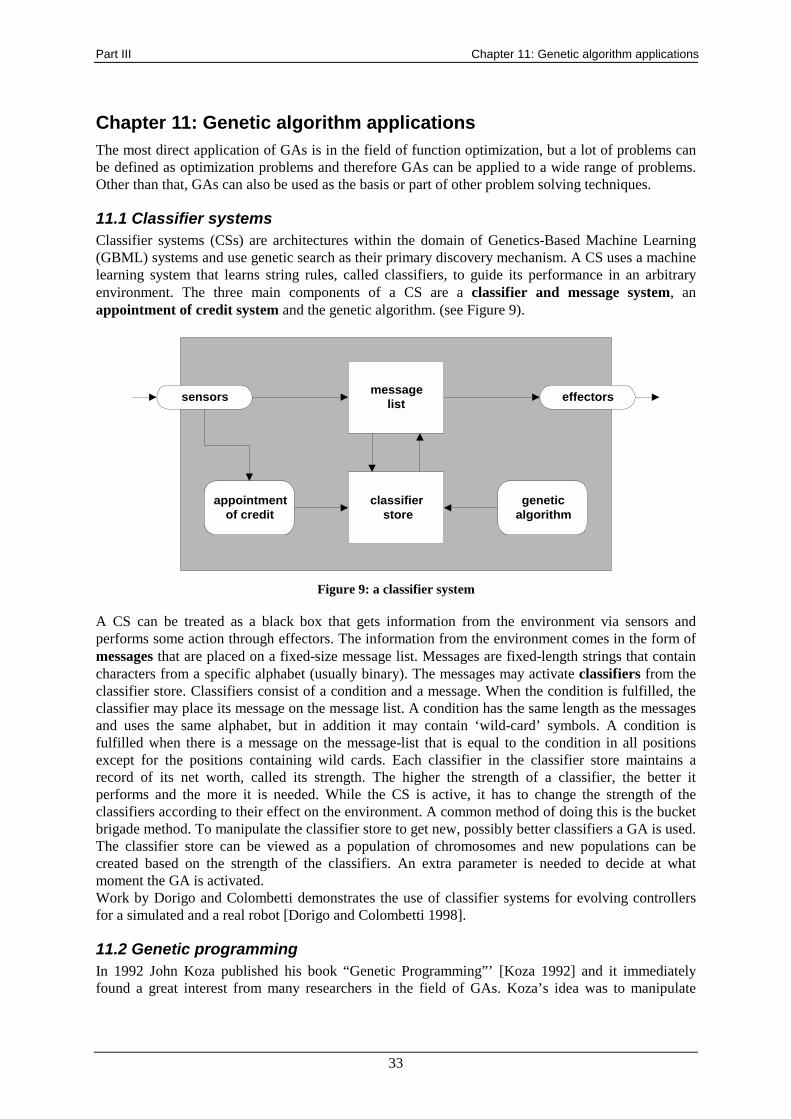
Part III Chapter 11: Genetic algorithm applications

33

Chapter 11: Genetic algorithm applications The most direct application of GAs is in the field of function optimization, but a lot of problems can be defined as optimization problems and therefore GAs can be applied to a wide range of problems. Other than that, GAs can also be used as the basis or part of other problem solving techniques.

11.1 Classifier systems Classifier systems (CSs) are architectures within the domain of Genetics-Based Machine Learning (GBML) systems and use genetic search as their primary discovery mechanism. A CS uses a machine learning system that learns string rules, called classifiers, to guide its performance in an arbitrary environment. The three main components of a CS are a classifier and message system, an appointment of credit system and the genetic algorithm. (see Figure 9).

sensors effectors

appointmentof credit

geneticalgorithm

messagelist

classifier store

Figure 9: a classifier system

A CS can be treated as a black box that gets information from the environment via sensors and performs some action through effectors. The information from the environment comes in the form of messages that are placed on a fixed-size message list. Messages are fixed-length strings that contain characters from a specific alphabet (usually binary). The messages may activate classifiers from the classifier store. Classifiers consist of a condition and a message. When the condition is fulfilled, the classifier may place its message on the message list. A condition has the same length as the messages and uses the same alphabet, but in addition it may contain ‘wild-card’ symbols. A condition is fulfilled when there is a message on the message-list that is equal to the condition in all positions except for the positions containing wild cards. Each classifier in the classifier store maintains a record of its net worth, called its strength. The higher the strength of a classifier, the better it performs and the more it is needed. While the CS is active, it has to change the strength of the classifiers according to their effect on the environment. A common method of doing this is the bucket brigade method. To manipulate the classifier store to get new, possibly better classifiers a GA is used. The classifier store can be viewed as a population of chromosomes and new populations can be created based on the strength of the classifiers. An extra parameter is needed to decide at what moment the GA is activated. Work by Dorigo and Colombetti demonstrates the use of classifier systems for evolving controllers for a simulated and a real robot [Dorigo and Colombetti 1998].

11.2 Genetic programming In 1992 John Koza published his book “Genetic Programming”’ [Koza 1992] and it immediately found a great interest from many researchers in the field of GAs. Koza’s idea was to manipulate

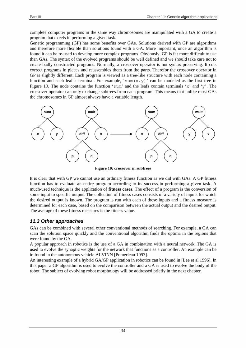
Part III Chapter 11: Genetic algorithm applications

34

complete computer programs in the same way chromosomes are manipulated with a GA to create a program that excels in performing a given task. Genetic programming (GP) has some benefits over GAs. Solutions derived with GP are algorithms and therefore more flexible than solutions found with a GA. More important, once an algorithm is found it can be re-used to develop more complex programs. Obviously, GP is far more difficult to use than GAs. The syntax of the evolved programs should be well defined and we should take care not to create badly constructed programs. Normally, a crossover operator is not syntax preserving. It cuts correct programs in pieces and reassembles them from the parts. Therefor the crossover operator in GP is slightly different. Each program is viewed as a tree-like structure with each node containing a function and each leaf a terminal. For example, ‘sum(x,y)’ can be modeled as the first tree in Figure 10. The node contains the function ‘sum’ and the leafs contain terminals ‘x’ and ‘y’. The crossover operator can only exchange subtrees from each program. This means that unlike most GAs the chromosomes in GP almost always have a variable length.

sum

x y

mult

xdiff

p q

sum

x y

mult

xdiff

p q

Figure 10: crossover in subtrees

It is clear that with GP we cannot use an ordinary fitness function as we did with GAs. A GP fitness function has to evaluate an entire program according to its success in performing a given task. A much-used technique is the application of fitness cases. The effect of a program is the conversion of some input to specific output. The collection of fitness cases consists of a variety of inputs for which the desired output is known. The program is run with each of these inputs and a fitness measure is determined for each case, based on the comparison between the actual output and the desired output. The average of these fitness measures is the fitness value.

11.3 Other approaches GAs can be combined with several other conventional methods of searching. For example, a GA can scan the solution space quickly and the conventional algorithm finds the optima in the regions that were found by the GA. A popular approach in robotics is the use of a GA in combination with a neural network. The GA is used to evolve the synaptic weights for the network that functions as a controller. An example can be in found in the autonomous vehicle ALVINN [Pomerleau 1993]. An interesting example of a hybrid GA/GP application in robotics can be found in [Lee et al 1996]. In this paper a GP algorithm is used to evolve the controller and a GA is used to evolve the body of the robot. The subject of evolving robot morphology will be addressed briefly in the next chapter.

Part III Chapter 12: Research questions

35

Chapter 12: Research questions Since several years, researchers have tried to use evolution for the automatic design of control systems for robots. The idea of evolutionary robotics is to use a GA or GP algorithm that evolves the control program depending on the task. However, the field of evolutionary robotics is still very young and practical applications are rare.

12.1 Fitness evaluation: real time or simulation? As with any genetic algorithm, a population has to be evaluated on the ability to perform the desired task. In the case of evolutionary robotics, the populations consist of robot control programs. A problem that needs to be resolved is the way that the evolving controllers can be evaluated best. If they are tested on real robots in the real world, then this has to be done in real-time and evolution will take very long. If controllers are tested using simulations the results may not be applicable on real robots because of the differences between the simulation and the real world. Simulations can be made more complex in order to represent the world more realistically, but this reduces the speed advantage that simulations have over real world evaluation. The problems with using physical robots are [Mataric and Cliff 1996]:

• Real time on real hardware: evolution on physical systems takes prohibitively long. • Battery lifetime: the unavoidable need to recharge robot batteries further slows down the

experimental procedure. • Physical hardware: aside from the prohibitive time overhead, the physical hardware of a

robotic system cannot survive the necessary continuous testing without constant maintenance and repairs.

Problems with using simulations:

• Noise and error models: since it is impossible to simulate all details of a physical system any abstraction made in a simulation may be exploited by the genetic algorithm and results in a behavior that is maladaptive in the real world.

• Generality v. usefulness: most successful simulations have been based on accurate physical measurements that were then incorporated into the sensor and effector models, as well as into the fitness function. This not only makes the job of writing a simulation for a nontrivial robot very challenging, it also produces an extremely specialized tool that does not generalize to any other system.

Although several attempts to evolve real robots in real-time were quite successful [Steels 1994], [Floreano and Mondada 1996] the simulation approach is more popular. A solution for better simulation-real world consistency and faster simulations might be the ‘minimal simulation’ method [Jakobi 1998] that focuses on making the simulation as simple as possible, but at the same time incorporating all the necessary conditions for the result to be usable on a real robot. This method appears to be promising, but so far it has only been used for relatively simple problems.

12.2 Design issues A feature of robotics that sets it apart from many other domains that use artificial evolution is noise. When working with robots or simulations that behave like real robots every evaluation function will be noisy. This makes comparisons between different controllers difficult and the individuals that receive the highest fitness values may not always be the fittest. One way of resolving this problem is to evaluate each individual a number of times, instead of just once, and take the average score as the its final fitness value. Obviously, this slows down the evolution process. Although evolutionary robotics is not restricted to any one particular type of controller some seem to perform better than others. The most commonly used types of control architectures in evolution are artificial neural networks [Floreano and Mondada 1996], Lisp or Lisp-like programs [Koza 1990], and classifier systems [Dorigo and Colombetti 1998]. Neural networks seem to be the most popular

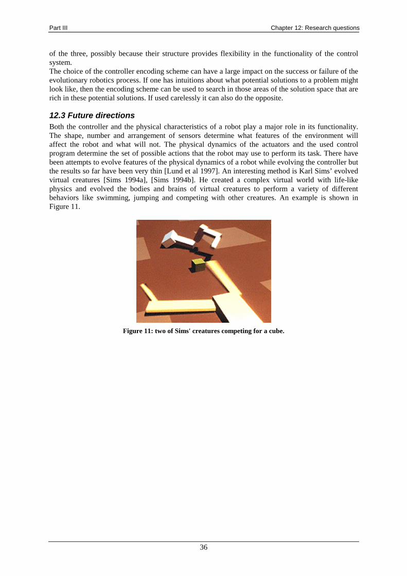
Part III Chapter 12: Research questions

36

of the three, possibly because their structure provides flexibility in the functionality of the control system. The choice of the controller encoding scheme can have a large impact on the success or failure of the evolutionary robotics process. If one has intuitions about what potential solutions to a problem might look like, then the encoding scheme can be used to search in those areas of the solution space that are rich in these potential solutions. If used carelessly it can also do the opposite.

12.3 Future directions Both the controller and the physical characteristics of a robot play a major role in its functionality. The shape, number and arrangement of sensors determine what features of the environment will affect the robot and what will not. The physical dynamics of the actuators and the used control program determine the set of possible actions that the robot may use to perform its task. There have been attempts to evolve features of the physical dynamics of a robot while evolving the controller but the results so far have been very thin [Lund et al 1997]. An interesting method is Karl Sims’ evolved virtual creatures [Sims 1994a], [Sims 1994b]. He created a complex virtual world with life-like physics and evolved the bodies and brains of virtual creatures to perform a variety of different behaviors like swimming, jumping and competing with other creatures. An example is shown in Figure 11.

Figure 11: two of Sims' creatures competing for a cube.

37

Bibliography

38

Bibliography Aleksander, I. and Morton, H. (1995) An introduction to neural computing. (2nd edition), International

Thomson Computer Press. Arkin, R. C. (1998) Behavior-based Robotics. The MIT Press, Cambridge, Massachusetts. Ballard, D.H. and Brown, C.M. (1982) Computer vision. Englewood Cliffs, N.J., Prentice-Hall. Braitenberg, V. (1984) Vehicles: experiments in synthetic psychology. The MIT Press, Cambridge

Massachusetts. Brady, M. (1985) Artificial intelligence and robotics. In Artificial Intelligence and Robotics, Vol. 26,

pages 79-121. Brooks, R.A. (1990) Elephants don't play chess. In Robotics and Autonomous Systems Vol. 6, 1990,

pages 3-15. Brooks, R.A. (1986) A robust layered control system for a mobile robot. MIT AI Lab Memo 864

September 1985, also IEEE Journal of Robotics and Automation Vol. 2, No. 1, March 1986, pages 14-23.

Connell, J.C. and Mahadevan, S. editors (1993) Robot learning, Kluwer Academic Publishers. Craig, J.J. (1989) Introduction to Robotics: mechanics and control (2nd edition), Addison-Wesley

Publishing Company, Inc. Dorigo, M. and Colombetti, M. (1998) Robot Shaping: an experiment in behavior engineering, The

MIT Press, Cambridge, Massachusetts. Floreano, D. and Mondada, F. (1996) Evolution of homing navigation in a real mobile robot. In IEEE

Transactions on Systems, Man and Cybernetics - Part B, Vol.26 (3), pages 396-407. Goldberg, D.E. (1989) Genetic algorithms in search, optimization and machine learning. Addison-

Wesley, Reading, Massachusetts. Haupt, R.L. and Haupt, S.E. (1998) Practical genetic algorithms. John Wiley & Sons. Hecht-Nielsen, R. (1989) Neurocomputing. Addison-Wesley Publishing Company, Inc. Holland, J.H. (1992) Adaptation in natural and artificial system. (2nd edition), The MIT Press,

Cambridge, Massachusetts, (1st edition 1975). Jakobi, N. (1998) Minimal solutions for evolutionary robotics. D. Phil Thesis, University of Sussex. Kortenkamp, D., Bonasso, R.P. and Murphy, R., editors (1998) Artificial intelligence and mobile

robots: case studies of successful robot systems. The MIT Press, Cambridge, Massachusetts. Koza, J.R. (1992) Genetic programming: on the programming of computers by means of natural

selection. MIT Press/Bradford Books Edition, Cambridge, Massachusetts.

Bibliography

39

Koza, J.R. (1990) Evolution and co-evolution of computer programs to control independently-acting agents. In From Animals to Animats: Proceedings of the First International Conference on Simulation of Adaptive Behavior, Meyer and Wilson editors, pages 366-375.

Koza, J.R. and Rice, J.P. (1992) Automatic programming of robots using genetic programming. In

Proceedings of the Tenth National Conference on Artificial Intelligence. Menlo Park, CA: AAAI Press / The MIT Press, pages 194-201.

Lee, W., Hallam, J. and Lund, H.H. (1996) A hybrid GP/GA approach for co-evolving controllers

and robot bodies to achieve fitness-specified tasks. In Proceedings of IEEE 3rd International Conference on Evolutionary Computation. IEEE Press.

Lund, H.H. and Miglino, O. (1998) Evolving and breeding robots. In Proceedings of the First

European Workshop on Evolutionary Robotics. Springer-Verlag. Lund, H.H., Hallam, J. and Lee, W. (1997) Evolving robot morphology. In Proceedings of IEEE 4th

International Conference on Evolutionary Computation. IEEE Press. Lund, H.H., Webb, B. and Hallam, J. (1998) Physical and temporal scaling considerations in a robot

model of cricket calling song preference. In Artificial Life 4, Vol. 1, pages 95-107, 1998. Also in Proceedings of Artificial Life VI.

MacLennan, B. (1991) Synthetic ethology: an approach to the study of communication. In Artificial

Life II: the Proceedings of the Second Workshop on the Synthesis and Simulation of Living Systems, Vol. 10. Santa Fe Institute Studies in the Sciences of Complexity, Redwood City, CA: Addison-Wesley, pages 631-658. Also University of Tennessee, Knoxville, Department of Computer Science, Technical report CS-90-104, May 1990.

Maes, P. and Brooks, R.A. (1990) Learning to coordinate behaviors. In Proceedings of AAAI-90,

pages 796-802. Mahadevan, S. and Connell, J. (1991) Automatic programming of behavior-based robots using

reinforcement learning. In Proceedings of the Ninth National Conference on Artificial Intelligence (AAAI ’91), Anaheim CA, July 1991, pages 768-773.

Mataric, M.J. (1994) Learning to behave socially. In proceedings of "From animals to animats 3,"

Third International Conference on Simulation of Adaptive Behavior (SAB-94). Cliff, D. et al. Editors, MIT Press, pages 453-462.

Mataric, M.J. (1992) Behavior-based systems: main properties and implications. In Proceeding of

the IEEE International Conference on Robotics and Automation, Workshop on Architectures for Intelligent Control Systems, Nice, France, May 1992, pages 46-54.

Mataric, M.J. and Cliff, D. (1996) Challengs in evolving controllers for physical robots. In

Evolutional Robotics; special issue of Robotics and Autonomous Systems, Vol. 19, No.1, Oct 1996, pages 67-83. Also Brandeis University Computer Science Technical Report CS-95-184, Nov 1995.

McFarland, D. (1981) The Oxford companion to animal behavior, Oxford University Press. Mitchell, T.M. (1997) Machine Learning, McGraw-Hill Companies, Inc.

Bibliography

40

Nilsson, N.J. (1969) A mobile automoton: an application of artificial intelligence techniques. In Proceedings of the International Joint Conference on Artificial Intelligence (IJCAI-69). Washington, D.C., May. Reprinted in Autonomous mobile robots. Vol. 2, Iyengar, S. and Elfes, A. editors, IEEE Computer society press, Los Alamitos, 1991, pages 233-244.

Pomerleau, D. (1993) Neural network perception for mobile robot guidance. Kluwer Academic

Publishers, Boston. Russell, S. and Norvig, P. (1995) Artificial Intelligence: a modern approach. Prenctice-Hall

International, Inc. Sims, K. (1994a) Evolving virtual creatures. In Computer graphics, proceedings of Siggraph July

’94, pages 15-22. Sims, K. (1994b) Evolving 3D morphology and behavior by competition. In Artificial Life IV

proceedings, Brooks, R. and Maes, P. editors, MIT Press, pages 28-39. Spronck, P. (1996) Elegance: genetic algorithms in reinforcement control. Master’s Thesis, Delft

University of Technology, The Netherlands. Steels, L. (1997) A selectionist mechanism for autonomous behavior acquisition. In Robotics and

Autonomous Systems, Vol 20, pages 117-131. Steels, L. (1994) Emergent functionality in robotic agents through on-line evolution. In Designing

Autonomous Agents. Edited Maes, P., MIT Press, Cambridge Massachusetts, pages 71-88.

Appendix Used WWW-pages

41

Appendix: Used WWW-pages Note: all addresses were checked august 27th 1999. A complete list of all addresses can also be found at http://student.twi.tudelft.nl/~s218303/robotlinks.html

People Arkin, Ronald http://www.cc.gatech.edu/aimosaic/faculty/arkin Bonasso, Pete http://tommy.jsc.nasa.gov/~bonasso Brooks, Rodney http://www.ai.mit.edu/people/brooks Channon, Alastair http://www.channon.net/alastair Dorigo, Marco http://iridia.ulb.ac.be/dorigo/dorigo.html Floreano, Dario http://diwww.epfl.ch/lami/team/floreano Forrest, Stephanie http://www.cs.unm.edu/~forrest Goldberg, David http://www.ge.uiuc.edu/people/faculty/Goldberg.html Harvey, Inman http://doc-sun.crn.cogs.susx.ac.uk/users/inmanh Husbands, Phil http://www.cogs.susx.ac.uk/users/philh Kaelbling, Leslie http://www.cs.brown.edu/people/lpk Koenig, Sven http://www.cc.gatech.edu/fac/Sven.Koenig Konolige, Kurt http://www.ai.sri.com/~konolige Kortenkamp, David http://tommy.jsc.nasa.gov/~korten Koza, John http://www.genetic-programming.com/johnkoza.html Krink, Thiemo http://www.daimi.aau.dk/~krink Kuipers, Benjamin http://www.cs.utexas.edu/users/kuipers/index.html Lund, Henrik http://www.daimi.au.dk/~hhl Maes, Pattie http://pattie.www.media.mit.edu/people/pattie/homepage.html Mahadevan, Sridhar http://www.cps.msu.edu/~mahadeva Martin, Fred http://lcs.www.media.mit.edu/people/fredm Mataric, Maja http://www-robotics.usc.edu/~maja McLennan, Bruce http://www.cs.utk.edu/~mclennan Minsky, Marvin http://minsky.www.media.mit.edu/people/minsky Mitchell, Melanie http://www.santafe.edu/~mm Mondada, Francesco http://diwww.epfl.ch/lami/team/mondada Nilsson, Nils http://robotics.stanford.edu/people/nilsson Nolfi, Stefano http://kant.irmkant.rm.cnr.it/nolfi.html Resnick, Mitchel http://mres.www.media.mit.edu/people/mres Rybski, Paul http://www-users.cs.umn.edu/~rybski Simmons, Reid http://www.cs.cmu.edu/~reids Sims, Karl http://www.genarts.com/karl Steels, Luc http://arti.vub.ac.be/steels Thrun, Sebastian http://www.cs.cmu.edu/~thrun

Robots Alvinn http://www.navlab.org/projects/ALVINN.html Flakey http://www.ai.sri.com/people/flakey Khep on the web http://KhepOnTheWeb.epfl.ch Marie Curie http://mars.jpl.nasa.gov/2001 Minerva http://www.cs.cmu.edu/~minerva Rhino http://www.informatik.uni-bonn.de/~rhino Sojourner http://mars.jpl.nasa.gov/default.html Xavier http://www.cs.cmu.edu/~xavier

Appendix Used WWW-pages

42

Research institutions University of Aarhus LEGO Lab http://legolab.daimi.aau.dk University of Amsterdam Intelligent Autonomous

Systems Group http://www.wins.uva.nl/research/ias

Boston University AI Laboratory http://neurobotics.bu.edu Free University of Brussel AI Laboratory http://arti.vub.ac.be California Institute of Technology Robotic’s

Homepage http://robby.caltech.edu

University of South California Robotics Institute http://www-robotics.usc.edu Carnegie Mellon University http://www.ri.cmu.edu University of Edingburgh Mobile Robots Group http://www.dai.ed.ac.uk/groups/mrg Georgia Institute of Technology Mobile Robot

Laboratory http://www.cc.gatech.edu/aimosaic/robot-lab

University of Illinois Genetic Algorithms Laboratory http://gal4.ge.uiuc.edu/illigal.home.html University of Manitoba Computational Intelligence

Laboratory http://www.ee.umanitoba.ca/~cilab

Massachusetts Institute of Technology AI Laboratory http://www.ai.mit.edu/projects Michigan State University Genetic Algorithms

Research and Applications Group http://GARAGe.cps.msu.edu

University of Minnesota AI, Robotics and Vision Laboratory

http://www.cs.umn.edu/Research/airvl

NASA’s Space Telerobotics Program Home Page http://ranier.hq.nasa.gov/telerobotics_page/telerobotics.shtm

SRI International's Artificial Intelligence Center http://www.ai.sri.com/ Stanford University Robotics Laboratory http://robotics.stanford.edu University of Western Australia Telerobot on the web http://telerobot.mech.uwa.edu.au University of Zurich Artificial Intelligence Laboratory http://www.ifi.unizh.ch/groups/ailab

Newsgroups Robotics FAQ http://www.frc.ri.cmu.edu/robotics-faq Robot Competition FAQ http://www.ncc.com/misc/rcfaq.html The Hitch-Hiker's Guide to Evolutionary

Computation (FAQ for comp.ai.genetic) http://www.cs.purdue.edu/coast/archive/clife/FAQ/www

News://comp.ai.alife News://comp.ai.genetic News://comp.robotics.misc News://comp.robotics.research

Software Saphira robot control system http://www.ai.sri.com/~konolige/saphira/ Genetic Programming for trail following ants http://members.xoom.com/lowht1 Genetic Algorithms and Artificial Life

resources http://www.scs.carleton.ca/~csgs/resources/gaal.html

Genetic Algorithms Software http://www.geneticprogramming.com/ga/Gasoftware.html The Genetic Algorithms Archive http://www.aic.nrl.navy.mil/galist Matthew's C++ Genetic Algorithm Library http://lancet.mit.edu/ga

Links to links Internet Robotic sources http://grouchy.cs.indiana.edu/usr/local/www/robotics/worl

d.html Ragman's robotic links http://www.euronet.nl/users/ragman/link_64.html Robot Information Central http://www.robotics.com/robots.html Robotics Internet Resources page http://www-robotics.cs.umass.edu/robotics.html Evolutionary computation and Artificial

Life http://www.dai.ed.ac.uk/groups/evalg/copy_of_smucker_ec_page.html

43