8945 2021

March 2021

The US-China Phase One Trade Deal: An Economic Analysis of the Managed Trade Agreement Michael Funke, Adrian Wende

Impressum:

CESifo Working Papers ISSN 2364-1428 (electronic version) Publisher and distributor: Munich Society for the Promotion of Economic Research - CESifo GmbH The international platform of Ludwigs-Maximilians University’s Center for Economic Studies and the ifo Institute Poschingerstr. 5, 81679 Munich, Germany Telephone +49 (0)89 2180-2740, Telefax +49 (0)89 2180-17845, email office@cesifo.de Editor: Clemens Fuest https://www.cesifo.org/en/wp An electronic version of the paper may be downloaded · from the SSRN website: www.SSRN.com · from the RePEc website: www.RePEc.org · from the CESifo website: https://www.cesifo.org/en/wp

CESifo Working Paper No. 8945

The US-China Phase One Trade Deal: An Economic

Analysis of the Managed Trade Agreement

Abstract In light of the recent tit-for-tat trade dispute between China and the US, interest in quantifying the effects of the so-called phase one agreement has risen. To this end, the paper quantifies the impact of the asymmetric managed trade agreement using such a multi-country open-economy dynamic general equilibrium model. Besides assessing the direct implications for China and the US, trade diversion effects are also analyzed. The model-based analysis finds noticeable positive (negative) impacts of the agreement for the US (China) as well as negative spillover effects for countries not directly affected by the managed trade deal due to trade diversion. The impact of possible future trade agreements is also examined.

JEL-Codes: F130, F410, F420.

Keywords: phase one deal, managed trade, open-economy dynamic general equilibrium model, United States, China.

Michael Funke

Department of Economics Hamburg University / Germany michael.funke@uni-hamburg.de

& Department of Economics and Finance

Tallinn University of Technology / Estonia michael.funke@taltech.ee

Adrian Wende Department of Economics

Hamburg University / Germany adrian.wende@wiso.uni-hamburg.de

March 2021

1

1. Introduction

After three years of tariffs and tensions whilst the US and China have grown more hostile to one another,

Chinese Vice Premier Liu He and US Trade Representative Robert Lighthizer signed the “Economic and

Trade Agreement” (ETA), also referred to as the US–China phase one trade deal on 15 January 2020.1 The

date of entry into force was 14 February 2020. The Agreement withholds further escalation of the on-and-

off trade war between the US and China. The bilateral deal has three main components: (i) Chinese

commitments to purchase more agricultural, energy and manufactured goods, and services; (ii) Chinese

commitments to reform investment policies and enforce intellectual property rights; and (iii) abstention

from currency manipulation. In addition, the trade deal comprises provisions to monitor the implementation

of the pact, settle disputes and pursue additional policy reforms in phase two.

The centerpiece of the trade deal consists of the introduction of a voluntary import expansion (VIE)

opening up the Chinese markets.2 Voluntary VIEs are ultimately the import counterpart to voluntary export

restraints (VERs). While a mandated market opening by means of a VIE sets a quantitative floor on China’s

imports, VERs would set a quantitative ceiling on the country’s exports. Obviously, this agreement has

provoked very varied sentiments across countries. The other World Trade Organisation (WTO) member

countries are wary and consider this is a worrisome message violating the most‐favored‐nations principle

and increasingly marginalizing the WTO. Multilateral liberalization is out and discriminatory bilateral

mercantilism is in. From the unilateral American viewpoint, things are different. Accordingly, the market-

opening VIE, tied to easily verifiable trade flows, is a necessity because of persistent and discriminatory

policy distortions and allegedly opaque and unfair Chinese trade barriers that cannot be addressed with

traditional rules-based trade policy tools. The VIE is also considered to prove Chinese good faith.3

To gauge the macroeconomic effects of the VIE agreement between the US and China, we develop an

open-economy dynamic general equilibrium model in the spirit of Ghironi and Melitz (2005). For the

research question at hand, however, the model is modified in several ways. First, the model is extended by a

third country and calibrated to represent the US, China and the rest of the world (RoW). Second, the China

module of the model also contains a state-owned enterprise sector operating under the authority of the

government. Third, tariffs are introduced as a policy instrument in all economies. Fourth, we adopt the

nested constant elasticity of substitution CES preferences proposed by Feenstra et al. (2018) to distinguish

1 For the text of the phase one trade agreement between the US government and the Chinese government, see https://ustr.gov/sites/default/files/files/agreements/phase%20one%20agreement/Economic_And_Trade_Agreement_Between_The_United_States_And_China_Text.pdf. 2 VIEs entered the lexicon of trade policy after Bhagwati’s (1987) pioneering article. Other seminal papers addressing various implications of VIEs, include Bagwell and Staiger (1990), Bjorksten (1994), Dinopoulos and Kreinin (1990), Ethier and Horn (1996) and Greaney (1996, 1999). For a thorough assessment of existing preferential trade agreements highlighting similarities and differences, see Mattoo et al. (2020). 3 Autor et al. (2020) and Colantone and Stanig (2018a) have established a causal link between the China import shock and a rise of political polarization in the US and an increasing support for right-wing populist parties in Europe. Colantone and Stanig (2018b) have further directly linked the China shock to the outcomes of the Brexit referendum vote.

2

between micro and macro trade elasticities. Finally, we include international production linkages through a

model structure similar to that of Caliendo et al. (2015).

To our knowledge, this is the first study that attempts to quantify the global impact of the US–China

managed trade agreement using such a multi-country open-economy dynamic general equilibrium model. A

partial list of other recent contributions includes Amiti et al. (2019), Cerutti et al. (2019), Chowdhry and

Felbermayr (2020a, 2020b), Freund et al. (2020) and Handley et al. (2020). Chowdhry and Felbermayr

(2020a, 2020b) employ an empirical gravity model disaggregated by sector to analyze the impact of the

trade agreement on third countries. On the contrary, Freund et al. (2020) use a calibrated computable

general equilibrium model under the assumption of perfect competition to analyze the resulting trade

patterns. The paper by Bolt et al. (2019) using the multiregional, general equilibrium model EAGLE is

from a methodological point of view closer to our exercise, but the outcome-based phase one trade

agreement is not evaluated. Finally, Cerutti et al. (2019) examine potential knock-on effects of the managed

trade agreement, which were still unknown at the time of writing and thus hypothetical, by means of

empirical modeling approaches. In general, one may say that our study fits into this emerging literature on

the re-emergence of discriminatory protectionism shaking the foundations of the global trading system.

The remainder of this paper is structured as follows. Section 2 explains the contents of the agreement and

analyzes its implementation to date. Section 3 lays out the modeling framework and research design.

Section 4 presents the model calibration, and Section 5 presents the various numerical trade policy

scenarios. In doing so, possible future trade arrangements will also be examined. Supplementing this,

Section 6 provides a welfare analysis. The last section concludes.

2. The Asymmetric Phase One Trade Agreement and its Implementation to Date

Chapter 6 of the phase one trade deal contains legal commitments for China to make additional purchases

of US exports in both 2020 and 2021 that would total USD 200 billion over its baseline purchases in 2017.

Those 2017 purchases were about USD 130 billion of US merchandize exports and USD 50 billion of US

service exports. Thus, the VIE agreement commits China to increase its imports from the US by no less

than 55 percent. Within the overall target there are four explicit subtargets for covered products in the

manufacturing, agricultural, energy, and services sectors.4

For the implementation of the ambitious commitments, the Chinese government has a variety of

enforcement mechanism options from which to choose. In particular, it could pressure its state-owned

enterprises (SOEs) by persuasion to allow greater imports of US products. In 2019, however, Chinese SOEs

purchased only 26 percent of Chinese total imports. The managed trade targets could therefore only be met

if the Chinese government somehow directs its SOEs to shift their 26 percent of imports entirely toward 4 Among the various types of VIE agreements (content VIE, market-share VIE and total value VIE), market-share VIEs have proven to be the most popular in practice. An important reason for this is that this form of VIE is susceptible to the rent-seeking of certain stakeholders (see, e.g., Rodrik, 2018). Grossman and Helpman (1994) have developed a model to explain the equilibrium structure of trade protection where special interest groups make political contributions in order to influence the government’s choice of trade policy.

3

American suppliers. Ultimately, one inconsistency of the agreement thus is that the special role of the

SOEs, which has been repeatedly criticized by the American authorities, is even strengthened by the trade

agreement.

As regards tariffs, the high level of tariffs achieved will largely be maintained. The US will cut by half the

tariff rate it imposed on 1 September 2019 on a USD 120 billion list of Chinese goods to 7.5%. US tariffs

of 25% USD 250 billion-worth of Chinese goods put in place earlier will remain unchanged. Tariffs that

were scheduled to go into effect on 15 December 2019 on nearly USD 160 billion-worth of Chinese goods,

including cellphones, laptop computers, toys and clothing, are suspended indefinitely. China’s retaliatory

15 December 2019 tariffs, including a 25% tariff on US cars have also been suspended. Overall, however,

reciprocal average tariffs will remain at a very elevated level for the foreseeable future.5 In addition, the

phase one deal did not even touch other contentious issues between the trade conflict, such as China’s SOEs

and subsidies. Moreover, with President Biden unlikely to go easy on China, these trade barriers are likely

to endure.

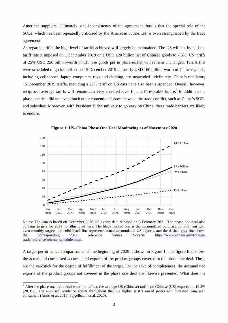
Figure 1: US–China Phase One Deal Monitoring as of November 2020

Notes: The data is based on December 2020 US export data released on 5 February 2021. The phase one deal also contains targets for 2021 not illustrated here. The black dashed line is the accumulated purchase commitment with even monthly targets, the solid black line represents actual accumulated US exports, and the dashed gray line shows the corresponding 2017 reference values. Source: https://www.census.gov/foreign-trade/reference/release_schedule.html.

A target-performance comparison since the beginning of 2020 is shown in Figure 1. The figure first shows

the actual and committed accumulated exports of the product groups covered in the phase one deal. These

are the yardstick for the degree of fulfillment of the target. For the sake of completeness, the accumulated

exports of the product groups not covered in the phase one deal are likewise presented. What does the

5 After the phase one trade deal went into effect, the average US (Chinese) tariffs on Chinese (US) exports are 19.3% (20.3%). The empirical evidence shows throughout that the higher tariffs raised prices and punished American consumers (Amiti et al. 2019; Fajgelbaum et al. 2020).

4

compliance with the managed trade deal obligations look like until December 2020? The target-

performance comparison for the covered goods reveals a degree of fulfillment of 63 percent (USD 89.6

billion/USD 143.3 billion) in the first 11 months.6

An obvious problem is that neither the phase one deal, nor Figure 1 account for the COVID-19 pandemic,

which has led to an unprecedented disruption to world trade, as production and consumption were scaled

back across the globe.

According to the “WTO Trade Barometer” (https://www.wto.org/english/res_e/statis_e/wtoi_e.htm), which

combines a variety of trade-related component indices into a single composite index, world merchandise

trade plummeted to historically unprecedented levels during the first COVID-19 lockdown in spring 2020.

Afterwards, world trade rebounded strongly. Furthermore, a variety of precautionary trade barriers were

launched at the beginning of 2020. Import barriers of medical products and other essential goods were

lowered, while at the same time restrictions on the exports of such goods were introduced. The mix of

import facilitation and export controls was driven by the objective of ensuring an adequate supply of

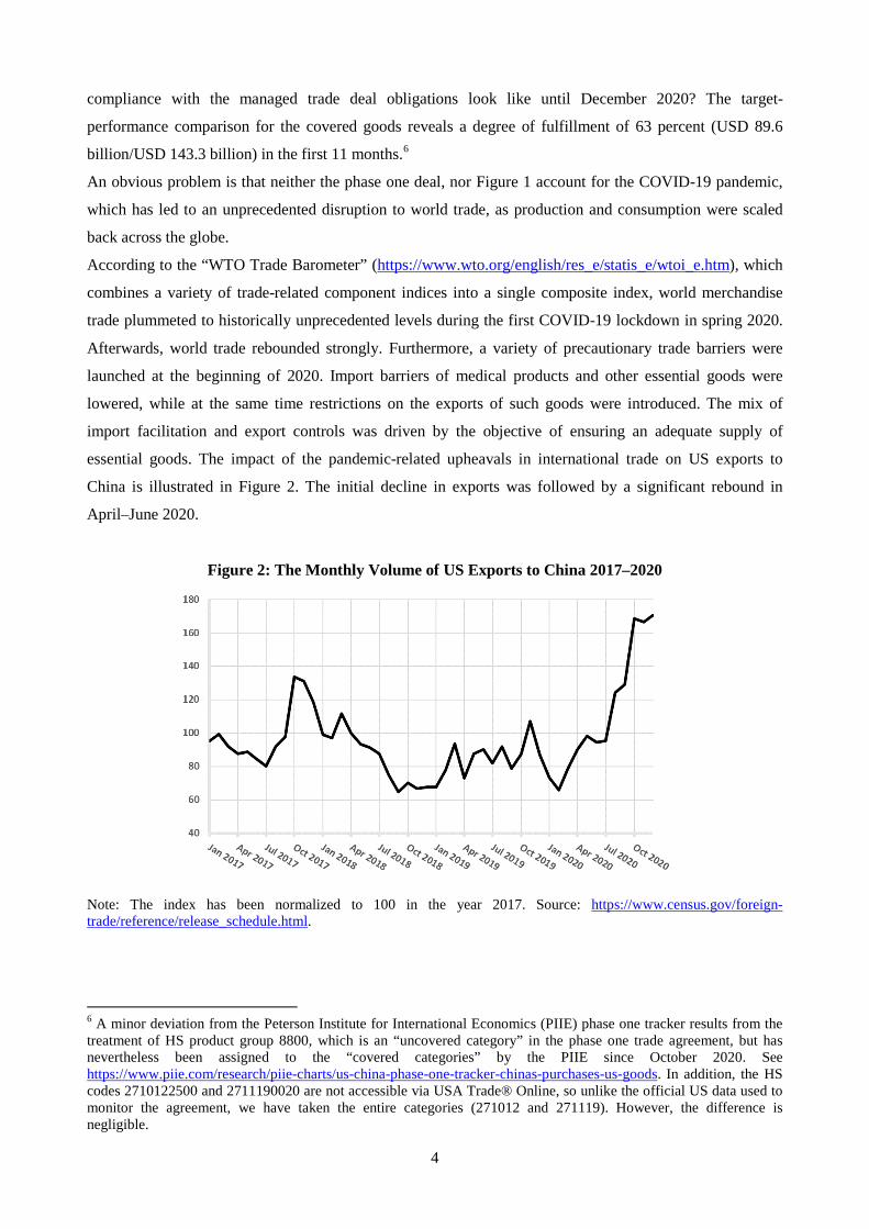
essential goods. The impact of the pandemic-related upheavals in international trade on US exports to

China is illustrated in Figure 2. The initial decline in exports was followed by a significant rebound in

April–June 2020.

Figure 2: The Monthly Volume of US Exports to China 2017–2020

Note: The index has been normalized to 100 in the year 2017. Source: https://www.census.gov/foreign-trade/reference/release_schedule.html.

6 A minor deviation from the Peterson Institute for International Economics (PIIE) phase one tracker results from the treatment of HS product group 8800, which is an “uncovered category” in the phase one trade agreement, but has nevertheless been assigned to the “covered categories” by the PIIE since October 2020. See https://www.piie.com/research/piie-charts/us-china-phase-one-tracker-chinas-purchases-us-goods. In addition, the HS codes 2710122500 and 2711190020 are not accessible via USA Trade® Online, so unlike the official US data used to monitor the agreement, we have taken the entire categories (271012 and 271119). However, the difference is negligible.

5

Remarkably, the agreement makes no mention of COVID-19, although the pandemic had already hit China

when the agreement came into force. The question of how the signatories will deal with this global shock is

currently pending.7 Against the backdrop of this uncertainty as to whether and, if so, how the pandemic will

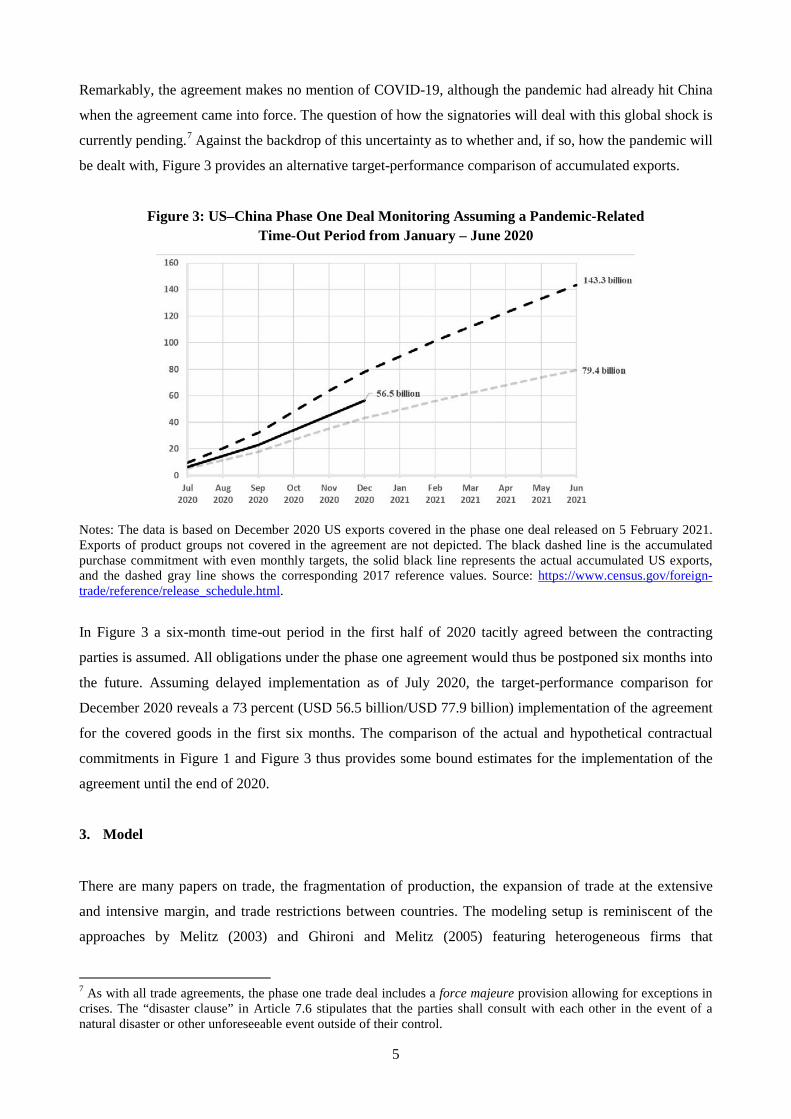
be dealt with, Figure 3 provides an alternative target-performance comparison of accumulated exports.

Figure 3: US–China Phase One Deal Monitoring Assuming a Pandemic-Related Time-Out Period from January – June 2020

Notes: The data is based on December 2020 US exports covered in the phase one deal released on 5 February 2021. Exports of product groups not covered in the agreement are not depicted. The black dashed line is the accumulated purchase commitment with even monthly targets, the solid black line represents the actual accumulated US exports, and the dashed gray line shows the corresponding 2017 reference values. Source: https://www.census.gov/foreign-trade/reference/release_schedule.html.

In Figure 3 a six-month time-out period in the first half of 2020 tacitly agreed between the contracting

parties is assumed. All obligations under the phase one agreement would thus be postponed six months into

the future. Assuming delayed implementation as of July 2020, the target-performance comparison for

December 2020 reveals a 73 percent (USD 56.5 billion/USD 77.9 billion) implementation of the agreement

for the covered goods in the first six months. The comparison of the actual and hypothetical contractual

commitments in Figure 1 and Figure 3 thus provides some bound estimates for the implementation of the

agreement until the end of 2020.

3. Model

There are many papers on trade, the fragmentation of production, the expansion of trade at the extensive

and intensive margin, and trade restrictions between countries. The modeling setup is reminiscent of the

approaches by Melitz (2003) and Ghironi and Melitz (2005) featuring heterogeneous firms that

7 As with all trade agreements, the phase one trade deal includes a force majeure provision allowing for exceptions in crises. The “disaster clause” in Article 7.6 stipulates that the parties shall consult with each other in the event of a natural disaster or other unforeseeable event outside of their control.

6

endogenously decide not only how much they produce and export, but also whether they enter the market or

export at all. The Melitz (2003) model can also be referred to as Krugman (1980) meets Hopenhayn

(1992).8 For an overview, Figure 4 sketches the general structure of the model. The model is designed to

investigate the underlying questions in a coherent multi-country framework rigorously, yet still be tractable

to obtain intuitive results.

Figure 4: The General Structure of the Modeling Framework

The model presumes a two-stage production process. In the first stage, heterogeneous firms use labor,

capital and final goods to produce tradable intermediate goods (see Section 3.1.2). These firms are

differentially productive, drawing their productivity from a Pareto distribution at their birth. Only the most

productive of them export their products abroad. The tradable goods from the first stage are bought by the

firms in the second stage. As a country-specific feature, state-owned enterprises are also modeled in China.

Only in China we assume that some of the second stage firms are owned by the government. These can be

directly ordered by the Chinese government to purchase, for example, a higher share of tradable goods from

the US (see Section 3.1.1). Firms in the second stage produce a homogeneous final product, which they in

turn sell to households as consumption and capital goods and to firms in the first stage as material inputs.

8 For a comprehensive and instructive review of the literature, see Redding (2011).

7

The households of the three countries are connected via the bond market. They smooth their consumption

over time, accumulate capital and supply a fixed amount of labor (see Section 3.2). For the sake of clarity,

the governments that pursue trade policy VIEs, tariffs, directives and possibly subsidies are not shown (see

Section 3.3). The details of the model are described next.

3.1 Firms

The structure of the production sector is similar to that of Caliendo et al. (2015). Deviating from this multi-

good modeling framework, however, the model presented here incorporates a special three-country-four-

sector structure. The three countries are the United States (US), China (CN) and the rest of the world

(RoW). Each of these countries has privately owned enterprises (POEs). In addition and exclusively, China

also has a state-owned enterprise (SOE) sector.

3.1.1 Final Goods Production and Managed Trade Policy

The economy is populated by final goods firms, indexed by sector 𝑠 ∈ {𝑃𝑃𝑃, 𝑆𝑃𝑃} and country 𝑖 ∈

{𝑈𝑆;𝐶𝐶;𝑅𝑅𝑅}. Using the Dixit–Stiglitz aggregator, and the superscripts s and i, the production of final

goods in period t is given by:

𝑄𝑡𝑖𝑖 = 𝑍𝑖,𝑡𝑖 ��1 − 𝛼𝑖𝑖�

1𝜔 �𝑄𝐷𝑖,𝑡

𝑖 �𝜔−1𝜔 + �𝛼𝑖𝑖�

1𝜔 �𝑄𝑋𝑖,𝑡

𝑖 �𝜔−1𝜔 �

𝜔𝜔−1

, (1)

where 𝑍𝑖,𝑡𝑖 is the productivity of final goods firms in country 𝑖 and sector 𝑠 and 𝛼𝑖𝑖 is the degree of

openness, and 𝜔 is the macro elasticity, i.e., the elasticity of substitution between the domestically

produced bundle of intermediate varieties,

𝑄𝐷𝑖,𝑡𝑖 = �∫ �𝑄𝐷𝑖,𝑡

𝑖 (𝜑)�𝜃−1 𝜃⁄

𝜑∈Φ 𝑑𝜑�𝜃 𝜃−1⁄

, (2)

where 𝑄𝐷,𝑡𝑖𝑖 (𝜑) represent the demand for variety 𝜑, and the foreign produced bundle 𝑄𝑋𝑖,𝑡

𝑖 . We normalize

the productivity of POEs to 1, while the Chinese SOEs have lower productivity. The foreign bundle is

given by:

𝑄𝑋𝑖,𝑡𝑖 = �� �𝜅𝑖

𝑖𝑖�1𝜃 �𝑄𝑋𝑖,𝑡

𝑖𝑖 �𝜃−1𝜃

𝑖≠𝑖

�

𝜃𝜃−1

, (3)

8

where 𝜅𝑖𝑖𝑖 denotes the utility weight of the CES index, 𝑄𝑋𝑖,𝑡

𝑖𝑖 = �∫ �𝑄𝑋𝑖,𝑡𝑖𝑖 (𝜑)�

𝜃−1 𝜃⁄

𝜑∈Φ 𝑑𝜑�𝜃 𝜃−1⁄

and 𝜃 is

the micro elasticity of substitution, which is the same for all goods. The introduction of these two distinct

substitution elasticities thereby follows Feenstra et al. (2018). The motivation is that substitution between

domestic and foreign goods may be more difficult than between different foreign goods. The CES-based

final price index is given by

𝑃𝑃𝑃,𝑡𝑖 = ��1 − 𝛼𝑖��𝑃𝐷𝑃𝑃,𝑡

𝑖,𝑛 �1−𝜔

+ 𝑎𝑖�𝑃𝑋𝑃𝑃,𝑡𝑖,𝑛 �

1−𝜔�

11−𝜔 , (4)

where 𝑃𝐷𝑃𝑃,𝑡𝑖,𝑛 = �∫ �𝑃𝐷𝑃𝑃,𝑡

𝑖,𝑛 (𝜑)�1−𝜃

𝜑∈Φ 𝑑𝜑�1 1−𝜃⁄

and 𝑃𝑋𝑃𝑃,𝑡𝑖,𝑛 = �∑ 𝜅𝑖𝑖 �𝑃𝑋𝑃𝑃,𝑡

𝑖𝑖 ,𝑛 �1−𝜃

𝑖≠𝑖 �1 1−𝜃⁄

are the nominal price

indices of the domestic varieties and of imported intermediates, respectively. 𝑃𝑋𝑃𝑃,𝑡𝑖𝑖,𝑛 = �∫ (1 +𝜑∈Φ

𝜏𝑡𝑖𝑖) �𝑃𝑋𝑃𝑃,𝑡

𝑖𝑖,𝑛 (𝜑)�1−𝜃

𝑑𝜑�1 1−𝜃⁄

is the price index of varieties from country 𝑗, which also depends on the trade

tariff 𝜏𝑡𝑖𝑖 levied by country 𝑖 on products of country 𝑗.

A specific feature of the model is that in China, in addition to private companies, state-owned enterprises

are also present. Without government intervention, these SOEs act exactly like the POEs. The cornerstone

of the phase one deal was a Chinese pledge to purchase further American exports over 2020 and 2021. But

curiously, the agreement makes no mention of Beijing committing to cut its tariffs to facilitate those

purchases. The only viable option for meeting the obligations thus is an administrative order requiring the

Chinese SOEs to make additional imports from the US.9 In terms of an equation, this relative demand for

US products by the Chinese SOEs Ψt is given as:

Ψt =𝑃𝑋𝑋𝑋𝑃,𝑡𝐶𝐶𝐶𝑋 𝑄𝑋𝑋𝑋𝑃,𝑡

𝐶𝐶𝐶𝑋

𝑃𝐷𝑋𝑋𝑃,𝑡𝐶𝐶 𝑄𝐷𝑋𝑋𝑃,𝑡

𝐶𝐶 + 𝑃𝑋𝑋𝑋𝑃,𝑡𝐶𝐶𝐶𝑋 𝑄𝑋𝑋𝑋𝑃,𝑡

𝐶𝐶𝐶𝑋 + 𝑃𝑋𝑋𝑋𝑃,𝑡𝐶𝐶𝐶𝐶𝐶 𝑄𝑋𝑋𝑋𝑃,𝑡

𝐶𝐶𝐶𝐶𝐶 =𝑃𝑋𝑋𝑋𝑃,𝑡𝐶𝐶𝐶𝑋 𝑄𝑋𝑋𝑋𝑃,𝑡

𝐶𝐶𝐶𝑋

𝑃 𝑋𝑋𝑃,𝑡𝐶𝐶 𝑄𝑋𝑋𝑃,𝑡

𝐶𝐶 (5)

Since the Chinese SOEs are less productive than POEs, the SOEs receive two kinds of government

subsidies for compensation. First, SOEs receive subsidies 𝜏𝐷𝑖𝐷,𝑡𝐶𝐶 for domestic market purchases. Thus, the

price index of Chinese domestic varieties sold to SOEs is given by

𝑃𝐷𝑋𝑋𝑃,𝑡𝑖,𝑛 = �� (1 − 𝜏𝐷𝑖𝐷,𝑡

𝐶𝐶 ) �𝑃𝐷𝑋𝑋𝑃,𝑡𝑖,𝑛 (𝜑)�

1−𝜃

𝜑∈Φ𝑑𝜑�

1 1−𝜃⁄

(6)

9 See https://www.piie.com/blogs/trade-and-investment-policy-watch/trumps-phase-one-deal-relies-chinas-state-owned-enterprises.

9

Moreover, we introduce a subsidy 𝜏𝑖𝐷,𝑡𝐶𝐶𝐶𝑋 to SOEs for importing US goods.10 The price index of varieties

from the US exported to China is thus given by

𝑃𝑋𝑃𝑃,𝑡𝐶𝐶𝐶𝑋,𝑛 = �∫ �1 + 𝜏𝑡𝐶𝐶𝐶𝑋 − 𝜏𝑖𝐷,𝑡

𝐶𝐶𝐶𝑋� �𝑃𝑋𝑋𝑋𝑃,𝑡𝐶𝐶𝐶𝑋,𝑛(𝜑)�

1−𝜃

𝜑∈Φ 𝑑𝜑�1 1−𝜃⁄

(7)

Both subsidies are modeled symmetrically to tariffs, i.e., Chinese households receive the difference

between tariff revenues and subsidy expenditures as a lump sum payment.

In the interest of a straightforward modeling, we assume that the relative SOE demand for US goods is

simply set exogenously by the Chinese authorities. From standard profit maximization, the demand

function for domestic goods is obtained as

𝑄𝐷𝑋𝑋𝑃,𝑡𝐶𝐶

𝑄𝑋𝑋𝑃,𝑡𝐶𝐶 = (1 − 𝛼𝐶𝐶)�

𝑃𝐷𝑋𝑋𝑃,𝑡𝐶𝐶

𝑃𝑋𝑋𝑃,𝑡𝐶𝐶 �

−𝜔

Ξ−𝜔 , (8)

and the demand for goods from the rest of the world is given by

𝑄𝑋𝑋𝑋𝑃,𝑡𝐶𝐶𝐶𝐶𝐶

𝑄𝑋𝑋𝑃,𝑡𝐶𝐶 = 𝛼𝐶𝐶𝜅𝐶𝐶𝑃𝐶 �

𝑃𝑋𝑋𝑋𝑃,𝑡𝐶𝐶𝐶𝐶𝐶

𝑃𝑋𝑋𝑃,𝑡𝐶𝐶 �

−𝜃𝑆𝑆𝑆

�𝑄𝑋𝑋𝑋𝑃,𝑡𝐶𝐶

𝛼𝐶𝐶𝑄𝑋𝑋𝑃,𝑡𝐶𝐶 �

𝜔−𝜃𝜔

Ξ−𝜃 , (9)

where Ξ is defined as

Ξ =1

(1 −Ψt)−

Ψt(1 −Ψt)

(𝜅𝐶𝐶𝐶𝑋)1𝜃 �

𝑄𝑋𝑋𝑋𝑃,𝑡𝐶𝐶𝐶𝑋

𝑄𝑋𝑋𝑋𝑃,𝑡𝐶𝐶 �

−1𝜃�𝑄𝑋𝑋𝑋𝑃,𝑡𝐶𝐶

𝛼𝑖𝑄𝑋𝑋𝑃,𝑡𝐹 �

−1𝜔 𝑃𝑋𝑋𝑃,𝑡𝐶𝐶

𝑃𝑋𝑋𝑋𝑃,𝑡𝐶𝐶𝐶𝑋 . (10)

Notice that the above-described term Ξ equals 1 if the relative demand Ψt exactly matches the

unconstrained CES demand function of the SOEs without government interventions. Therefore, we rewrite

the demand policy of the Chinese government equivalently as:

Ψt = max� 𝛼𝐶𝐶𝜅𝐶𝐶𝐶𝑋 �𝑃𝑋𝑋𝑋𝑃,𝑡𝐶𝐶𝐶𝑋

𝑃𝑋𝑋𝑃,𝑡𝐶𝐶 �

1−𝜃

�𝑄𝑋𝑋𝑋𝑃,𝑡𝐶𝐶

𝛼𝐶𝐶𝑄𝑋𝑋𝑃,𝑡𝐶𝐶 �

𝜔−𝜃𝜔

,𝛹𝑡� (11)

10 The modeling illustrates an important issue. The phase one deal worsens rather than resolves one of the frictions underlying this trade conflict. The counterproductive trade agreement pushes China even farther away from markets and toward a state-driven economy. In practical terms, the Chinese authorities could promise to rebate the tariffs it collects on SOE purchases.

10

The first term in parentheses is the unconstrained CES-based demand function and Ψ𝑡 is the relative

minimum import quota for US goods set by the Chinese authorities. If the latter is not binding, then Ψt is

exactly the unrestricted demand for US goods.

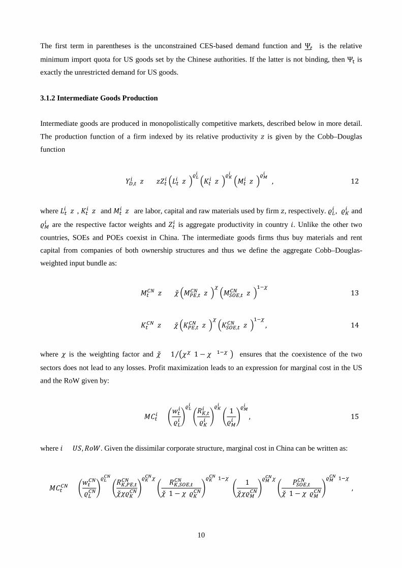
3.1.2 Intermediate Goods Production

Intermediate goods are produced in monopolistically competitive markets, described below in more detail.

The production function of a firm indexed by its relative productivity 𝑧 is given by the Cobb–Douglas

function

𝑌𝐷,𝑡𝑖 (𝑧) = 𝑧𝑍𝑡𝑖 �𝐿𝑡𝑖 (𝑧)�

𝜚𝐿𝑖

�𝐾𝑡𝑖(𝑧)�𝜚𝐾𝑖

�𝑀𝑡𝑖(𝑧)�

𝜚𝑀𝑖

, (12)

where 𝐿𝑡𝑖 (𝑧), 𝐾𝑡𝑖(𝑧) and 𝑀𝑡𝑖(𝑧) are labor, capital and raw materials used by firm 𝑧, respectively. 𝜚𝐿𝑖 , 𝜚𝐾𝑖 and

𝜚𝑀𝑖 are the respective factor weights and 𝑍𝑡𝑖 is aggregate productivity in country 𝑖. Unlike the other two

countries, SOEs and POEs coexist in China. The intermediate goods firms thus buy materials and rent

capital from companies of both ownership structures and thus we define the aggregate Cobb–Douglas-

weighted input bundle as:

𝑀𝑡𝐶𝐶(𝑧) = �̌� �𝑀𝑃𝑃,𝑡

𝐶𝐶 (𝑧)�𝜒�𝑀𝑋𝑋𝑃,𝑡

𝐶𝐶 (𝑧)�1−𝜒

(13)

𝐾𝑡𝐶𝐶(𝑧) = �̌� �𝐾𝑃𝑃,𝑡𝐶𝐶 (𝑧)�

𝜒�𝐾𝑋𝑋𝑃,𝑡

𝐶𝐶 (𝑧)�1−𝜒

, (14)

where 𝜒 is the weighting factor and �̌� = 1 �𝜒𝜒(1− 𝜒)(1−𝜒)�⁄ ensures that the coexistence of the two

sectors does not lead to any losses. Profit maximization leads to an expression for marginal cost in the US

and the RoW given by:

𝑀𝐶𝑡𝑖 = �𝑤𝑡𝑖

𝜚𝐿𝑖�𝜚𝐿𝑖

�𝑅𝐾,𝑡𝑖

𝜚𝐾𝑖�𝜚𝐾𝑖

�1𝜚𝑀𝑖�𝜚𝑀𝑖

, (15)

where 𝑖 = 𝑈𝑆,𝑅𝑅𝑅. Given the dissimilar corporate structure, marginal cost in China can be written as:

𝑀𝐶𝑡𝐶𝐶 = �𝑤𝑡𝐶𝐶

𝜚𝐿𝐶𝐶�𝜚𝐿𝐶𝐶

�𝑅𝐾,𝑃𝑃,𝑡𝐶𝐶

�̌�𝜒𝜚𝐾𝐶𝐶�𝜚𝐾𝐶𝐶𝜒

�𝑅𝐾,𝑋𝑋𝑃,𝑡𝐶𝐶

�̌�(1 − 𝜒)𝜚𝐾𝐶𝐶�𝜚𝐾𝐶𝐶(1−𝜒)

�1

�̌�𝜒𝜚𝑀𝐶𝐶�𝜚𝑀𝐶𝐶𝜒

�𝑃𝑋𝑋𝑃,𝑡𝐶𝐶

�̌�(1 − 𝜒)𝜚𝑀𝐶𝐶�𝜚𝑀𝐶𝐶(1−𝜒)

,

11

(16)

where 𝑤𝑡𝑖 denotes the real wage in country 𝑖, 𝑅𝐾,𝑡

𝐶𝐶 is the rental price of physical capital and 𝑃𝑋𝑋𝑃,𝑡𝐶𝐶 is the

price of the homogeneous final product produced by the state-owned enterprises in China and used as raw

material input by the intermediate firms. The POE final good price serves as numeraire and is normalized to

1. Note that 𝑀𝐶𝑡𝑖 is the marginal cost of buying an additional unit of the factor input bundle, which is the

same for all firms in country 𝑖, and not the marginal cost of producing an additional unit of output, which

varies across firms depending on their relative productivity z.

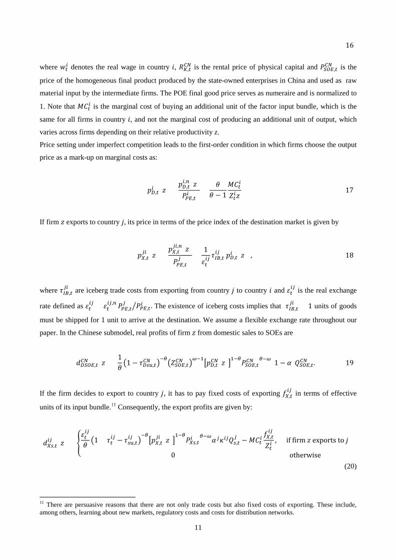
Price setting under imperfect competition leads to the first-order condition in which firms choose the output

price as a mark-up on marginal costs as:

𝑝𝐷,𝑡𝑖 (𝑧) =

𝑝𝐷,𝑡𝑖,𝑛(𝑧)𝑃𝑃𝑃,𝑡𝑖 =

𝜃𝜃 − 1

𝑀𝐶𝑡𝑖

𝑍𝑡𝑖𝑧 (17)

If firm 𝑧 exports to country 𝑗, its price in terms of the price index of the destination market is given by

𝑝𝑋,𝑡𝑖𝑖 (𝑧) =

𝑝𝑋,𝑡𝑖𝑖,𝑛(𝑧)

𝑃𝑃𝑃,𝑡𝑖 =

1𝜀𝑡𝑖𝑖 𝜏𝐼𝐼,𝑡

𝑖𝑖 𝑝𝐷,𝑡𝑖 (𝑧) , (18)

where 𝜏𝐼𝐼,𝑡𝑖𝑖 are iceberg trade costs from exporting from country 𝑗 to country 𝑖 and 𝜀𝑡

𝑖𝑖 is the real exchange

rate defined as 𝜀𝑡𝑖𝑖 = 𝜀𝑡

𝑖𝑖,𝑛 𝑃𝑃𝑃,𝑡𝑖 𝑃𝑃𝑃,𝑡

𝑖� . The existence of iceberg costs implies that 𝜏𝐼𝐼,𝑡𝑖𝑖 > 1 units of goods

must be shipped for 1 unit to arrive at the destination. We assume a flexible exchange rate throughout our

paper. In the Chinese submodel, real profits of firm 𝑧 from domestic sales to SOEs are

𝑑𝐷𝑋𝑋𝑃,𝑡𝐶𝐶 (𝑧) =

1𝜃 �

1 − 𝜏𝐷𝑖𝐷,𝑡𝐶𝐶 �−𝜃�𝑍𝑋𝑋𝑃,𝑡

𝐶𝐶 �𝜔−1�𝑝𝐷,𝑡𝐶𝐶(𝑧)�1−𝜃𝑃𝑋𝑋𝑃,𝑡

𝐶𝐶 𝜃−𝜔(1 − 𝛼)𝑄𝑋𝑋𝑃,𝑡𝐶𝐶 . (19)

If the firm decides to export to country 𝑗, it has to pay fixed costs of exporting 𝑓𝑋,𝑡𝑖𝑖 in terms of effective

units of its input bundle.11 Consequently, the export profits are given by:

𝑑𝑋𝑖,𝑡𝑖𝑖 (𝑧) = �

𝜀𝑡𝑖𝑖

𝜃 �1 + 𝜏𝑡𝑖𝑖 − 𝜏𝑖𝐷,𝑡

𝑖𝑖 �−𝜃�𝑝𝑋,𝑡

𝑖𝑖 (𝑧)�1−𝜃

𝑃𝑋𝑖,𝑡𝑖 𝜃−𝜔𝛼𝑖𝜅𝑖𝑖𝑄𝑖,𝑡

𝑖 − 𝑀𝐶𝑡𝑖𝑓𝑋,𝑡𝑖𝑖

𝑍𝑡𝑖, if firm 𝑧 exports to 𝑗

0 otherwise

(20)

11 There are persuasive reasons that there are not only trade costs but also fixed costs of exporting. These include, among others, learning about new markets, regulatory costs and costs for distribution networks.

12

Notice that, in China, intermediate firms make domestic profits from selling to the POE and the SOE sector.

In the US and the RoW a firm z decides separately whether and if so to which Chinese sectors it exports.

Hence, the total profits of firm z, the sum of its domestic and export profits, also have to be summed across

sectors, i.e., 𝑑𝑡𝑖(𝑧) = ∑ ∑ �𝑑𝐷𝑖,𝑡𝑖 (𝑧) + 𝑑𝑋𝑖,𝑡

𝑖𝑖 (𝑧)�𝑖≠𝑖𝑖 .

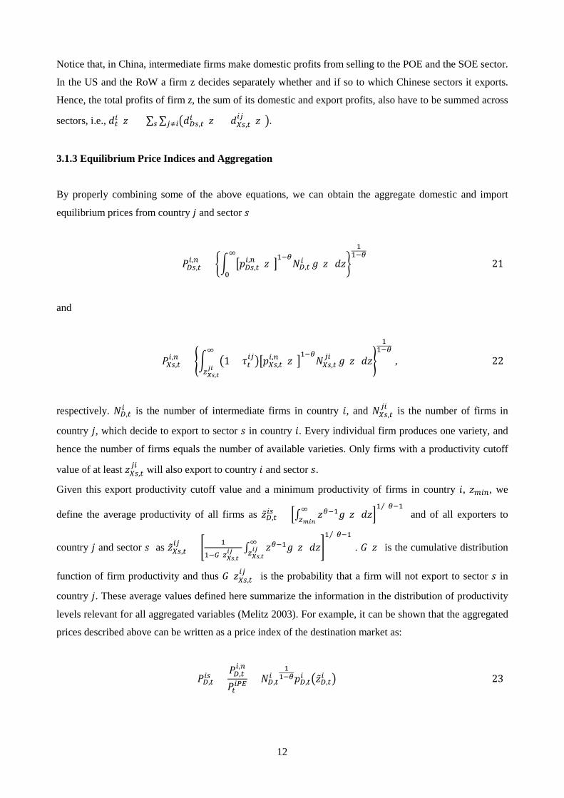
3.1.3 Equilibrium Price Indices and Aggregation

By properly combining some of the above equations, we can obtain the aggregate domestic and import

equilibrium prices from country 𝑗 and sector 𝑠

𝑃𝐷𝑖,𝑡𝑖,𝑛 = �� �𝑝𝐷𝑖,𝑡

𝑖,𝑛 (𝑧)�1−𝜃

𝐶𝐷,𝑡𝑖

∞

0𝑔(𝑧) 𝑑𝑧�

11−𝜃

(21)

and

𝑃𝑋𝑖,𝑡𝑖,𝑛 = �� �1 + 𝜏𝑡

𝑖𝑖��𝑝𝑋𝑖,𝑡𝑖,𝑛 (𝑧)�

1−𝜃𝐶𝑋𝑖,𝑡𝑖𝑖

∞

𝑧𝑋𝑋,𝑡𝑗𝑖

𝑔(𝑧) 𝑑𝑧�

11−𝜃

, (22)

respectively. 𝐶𝐷,𝑡𝑖 is the number of intermediate firms in country 𝑖, and 𝐶𝑋𝑖,𝑡

𝑖𝑖 is the number of firms in

country 𝑗, which decide to export to sector 𝑠 in country 𝑖. Every individual firm produces one variety, and

hence the number of firms equals the number of available varieties. Only firms with a productivity cutoff

value of at least 𝑧𝑋𝑖,𝑡𝑖𝑖 will also export to country 𝑖 and sector 𝑠.

Given this export productivity cutoff value and a minimum productivity of firms in country 𝑖, 𝑧𝑚𝑖𝑛, we

define the average productivity of all firms as �̃�𝐷,𝑡𝑖𝑖 = �∫ 𝑧𝜃−1𝑔(𝑧) 𝑑𝑧∞

𝑧𝑚𝑖𝑚�1 (𝜃−1)⁄

and of all exporters to

country 𝑗 and sector 𝑠 as �̃�𝑋𝑖,𝑡𝑖𝑖 = � 1

1−𝐺(𝑧𝑋𝑋,𝑡𝑖𝑗 )

∫ 𝑧𝜃−1𝑔(𝑧) 𝑑𝑧∞𝑧𝑋𝑋,𝑡𝑖𝑗 �

1 (𝜃−1)⁄

. 𝐺(𝑧) is the cumulative distribution

function of firm productivity and thus 𝐺(𝑧𝑋𝑖,𝑡𝑖𝑖 ) is the probability that a firm will not export to sector 𝑠 in

country 𝑗. These average values defined here summarize the information in the distribution of productivity

levels relevant for all aggregated variables (Melitz 2003). For example, it can be shown that the aggregated

prices described above can be written as a price index of the destination market as:

𝑃𝐷,𝑡𝑖𝑖 =

𝑃𝐷,𝑡𝑖,𝑛

𝑃𝑡𝑖𝑃𝑃= 𝐶𝐷,𝑡

𝑖1

1−𝜃𝑝𝐷,𝑡𝑖 ��̃�𝐷,𝑡

𝑖 � (23)

13

𝑃𝑋𝑖,𝑡𝑖𝑖 =

𝑃𝑋𝑖,𝑡𝑖𝑖,𝑛

𝑃𝑃𝑃,𝑡𝑖 = �1 + 𝜏𝑖

𝑖𝑖�𝐶𝑋𝑖,𝑡𝑖𝑖

11−𝜃𝑝𝐷,𝑡

𝑖 ��̃�𝑋𝑖,𝑡𝑖𝑖 � (24)

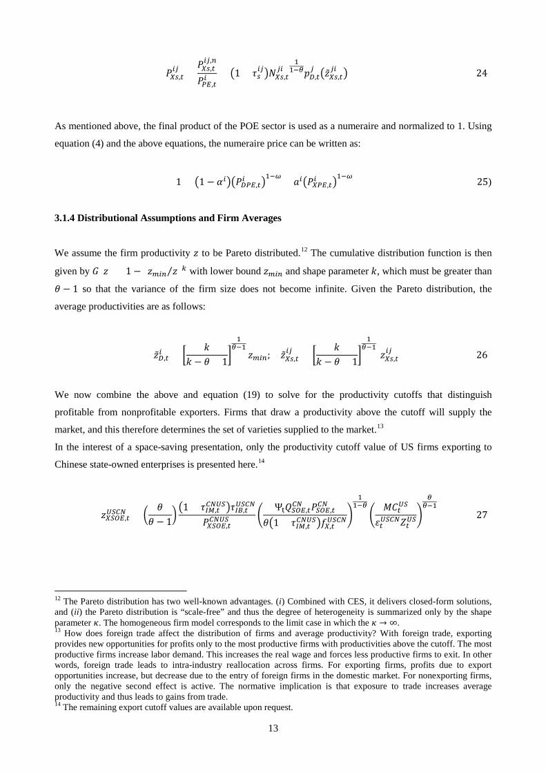
As mentioned above, the final product of the POE sector is used as a numeraire and normalized to 1. Using

equation (4) and the above equations, the numeraire price can be written as:

1 = �1 − 𝛼𝑖��𝑃𝐷𝑃𝑃,𝑡𝑖 �1−𝜔 + 𝑎𝑖�𝑃𝑋𝑃𝑃,𝑡

𝑖 �1−𝜔 (25)

3.1.4 Distributional Assumptions and Firm Averages

We assume the firm productivity 𝑧 to be Pareto distributed.12 The cumulative distribution function is then

given by 𝐺(𝑧) = 1 − (𝑧𝑚𝑖𝑛 𝑧⁄ )𝑘 with lower bound 𝑧𝑚𝑖𝑛 and shape parameter 𝑘, which must be greater than

𝜃 − 1 so that the variance of the firm size does not become infinite. Given the Pareto distribution, the

average productivities are as follows:

�̃�𝐷,𝑡𝑖 = �

𝑘𝑘 − 𝜃 + 1�

1𝜃−1

𝑧𝑚𝑖𝑛; �̃�𝑋𝑖,𝑡𝑖𝑖 = �

𝑘𝑘 − 𝜃 + 1�

1𝜃−1

𝑧𝑋𝑖,𝑡𝑖𝑖 (26)

We now combine the above and equation (19) to solve for the productivity cutoffs that distinguish

profitable from nonprofitable exporters. Firms that draw a productivity above the cutoff will supply the

market, and this therefore determines the set of varieties supplied to the market.13

In the interest of a space-saving presentation, only the productivity cutoff value of US firms exporting to

Chinese state-owned enterprises is presented here.14

𝑧𝑋𝑋𝑋𝑃,𝑡𝐶𝑋𝐶𝐶 = �

𝜃𝜃 − 1

��1 + 𝜏𝐼𝑀,𝑡

𝐶𝐶𝐶𝑋�𝜏𝐼𝐼,𝑡𝐶𝑋𝐶𝐶

𝑃𝑋𝑋𝑋𝑃,𝑡𝐶𝐶𝐶𝑋 �

Ψt𝑄𝑋𝑋𝑃,𝑡𝐶𝐶 𝑃𝑋𝑋𝑃,𝑡

𝐶𝐶

𝜃�1 + 𝜏𝐼𝑀,𝑡𝐶𝐶𝐶𝑋�𝑓𝑋,𝑡

𝐶𝑋𝐶𝐶�

11−𝜃

�𝑀𝐶𝑡𝐶𝑋

𝜀𝑡𝐶𝑋𝐶𝐶𝑍𝑡𝐶𝑋�

𝜃𝜃−1

(27)

12 The Pareto distribution has two well-known advantages. (i) Combined with CES, it delivers closed-form solutions, and (ii) the Pareto distribution is “scale-free” and thus the degree of heterogeneity is summarized only by the shape parameter 𝜅. The homogeneous firm model corresponds to the limit case in which the 𝜅 → ∞. 13 How does foreign trade affect the distribution of firms and average productivity? With foreign trade, exporting provides new opportunities for profits only to the most productive firms with productivities above the cutoff. The most productive firms increase labor demand. This increases the real wage and forces less productive firms to exit. In other words, foreign trade leads to intra-industry reallocation across firms. For exporting firms, profits due to export opportunities increase, but decrease due to the entry of foreign firms in the domestic market. For nonexporting firms, only the negative second effect is active. The normative implication is that exposure to trade increases average productivity and thus leads to gains from trade. 14 The remaining export cutoff values are available upon request.

14

It is straightforward to see that 𝜕𝑧𝑋𝑋𝑋𝑃,𝑡𝐶𝑋𝐶𝐶 𝜕Ψt⁄ = 𝑧𝑋𝑋𝑋𝑃,𝑡

𝐶𝑋𝐶𝐶 (1 − 𝜃)Ψt⁄ < 0, if the markup is positive and not

infinite, i.e., if 𝜃 > 1. A higher (relative) demand of the Chinese SOEs for US goods leads to a lower

productivity cutoff value and thus to lower average productivity of the respective US exporters, as firms

that are less productive self-select into the export market. The reason for this selection effect, as Caliendo et

al. (2015) call it, is that US exporters can spread their fixed costs over higher sales.

There are 𝐶𝐷,𝑡𝑖 companies in country 𝑖, but only 𝐶𝑋𝑖,𝑡

𝑖𝑖 companies decide to export to sector 𝑠 of country 𝑗.15

The share of the latter can be expressed by:

𝐶𝑋𝑖,𝑡𝑖𝑖

𝐶𝐷,𝑡𝑖 = �

𝑧𝑚𝑖𝑛

�̃�𝑋𝑖,𝑡𝑖𝑖 �

𝑘

�𝑘

𝑘 − 𝜃 + 1�

𝑘𝜃−1

(28)

The associated average profits are �̃�𝐷,𝑡𝑖 = 𝑑𝐷,𝑡

𝑖 (𝑧𝑚𝑖𝑛)[𝑘 (𝑘 − 𝜃 + 1)⁄ ] and

�̃�𝑋𝑖,𝑡𝑖𝑖 = [(𝜃 − 1) (𝑘 − 𝜃 + 1)⁄ ]𝑀𝐶𝑡𝑖 𝑓𝑋

𝑖𝑖𝑖 𝑍𝑡𝑖� , respectively. Average total profits of Chinese intermediate

firms are

�̃�𝑡𝐶𝐶 = �̃�𝐷,𝑡𝐶𝐶 + �̃�𝑋𝑋𝑃,𝑡

𝐶𝐶 + �𝐶𝑋𝑃𝑃,𝑡𝐶𝐶𝑖

𝐶𝐷,𝑡𝐶𝐶

𝑖≠𝐶𝐶

�̃�𝑋𝑃𝑃,𝑡𝐶𝐶𝑖 (29)

and for all 𝑖 ≠ 𝐶𝐶

�̃�𝑡𝑖 = �̃�𝐷,𝑡𝑖 +

𝐶𝑋𝑋𝑃,𝑡𝑖𝐶𝐶

𝐶𝐷,𝑡𝑖 �̃�𝑋𝑋𝑃,𝑡

𝑖𝐶𝐶 + �𝐶𝑋𝑃𝑃,𝑡𝑖𝑖

𝐶𝐷,𝑡𝑖

𝑖≠𝑖

�̃�𝑋𝑃𝑃,𝑡𝑖𝑖 (30)

3.1.5 Firm Entry and Exit Decisions

There is a large (unbounded) pool of prospective entrants into the industry. Prior to entry, firms are

identical. However, the entry decision undertaken by each firm is risky. When entering the market, identical

firms have to pay sunk entry costs amounting to 𝑓𝑃𝑖 effective units of the input bundle. Subsequent to the

market entry, the firm draws its productivity level z from the Pareto distribution described above. Prior to

entry, firms think about their expected profits and calculate the present value of the expected stream of

average profits starting in period 𝑡 + 1:

15 Since the firm draws its productivity and then decides whether or not it exports, all exporting firms must sell domestically (but the converse is not true).

15

𝜈�𝑡𝑖 = 𝑃𝑡 � [𝛽(1 − 𝛿)]ℎ−𝑡 �𝜆ℎ𝑖

𝜆𝑡𝑖� �̃�ℎ𝑖

∞

ℎ=𝑡+1

(31)

The expected stream of profits has to be equal to the costs of entry, which implies:

𝜈�𝑡𝑖 =𝑀𝐶𝑡𝑖𝑓𝑃𝑖

𝑍𝑡𝑖 (32)

As in Ghironi and Melitz (2005), new entrants in period 𝑡 start to produce in period 𝑡 + 1 and survive every

period with a probability (1 − 𝛿). Let the number of new entrants in period 𝑡 be 𝐶𝑃,𝑡𝑖 , then the stock of

firms is given by:

𝐶𝐷,𝑡𝑖 = (1 − 𝛿)�𝐶𝐷,𝑡−𝑡

𝑖 + 𝐶𝑃,𝑡−1𝑖 � (33)

3.2 The Representative Household

The representative household ℎ in country 𝑖 ∈ {𝑈𝑆;𝐶𝐶;𝑃𝑈} acts competitively, taking prices and policy as

given, and maximizes its utility

𝑉0 = 𝑃0 ��𝛽𝑡�𝐶ℎ,𝑡

𝑖 �1−𝛾

1 − 𝛾

∞

𝑡=0

� , (34)

where 𝑃0 is the rational expectations operator, 𝛽 is the discount factor and 𝛾 is the inverse elasticity of

intertemporal substitution with regard to consumption 𝐶ℎ,𝑡𝑖 . In the US and the RoW, households consume

POE-produced goods, i.e., 𝐶ℎ,𝑡𝑖 = 𝐶ℎ,𝑃𝑃,𝑡

𝑖 for 𝑖 ≠ 𝐶𝐶. In contrast, Chinese households consume a bundle of

POE-produced and SOE-produced goods 𝐶ℎ,𝑡𝐶𝐶 = �̌��𝐶ℎ,𝑃𝑃,𝑡

𝐶𝐶 �𝜒�𝐶ℎ,𝑋𝑋𝑃,𝑡𝐶𝐶 �1−𝜒. Consumption of country

𝑖 ≠ 𝑈𝑆 has a mass relative to the size of the US economy 𝜉𝐶𝑋. Therefore, all absolute quantities represent

aggregates relative to the US. Due to symmetry, consumption and labor supply are the same for every

household and, thus, 𝐶ℎ,𝑖,𝑡𝑖 = 𝜉𝑈𝑆

𝜉𝑖𝐶𝑖,𝑡𝑖 . The aggregated budget constraint of all households in country 𝑖 is

given by:

� 𝐵𝑖,𝑡𝑖𝑖

𝑖≠ 𝑖 + � 𝜀𝑡

𝑖𝑖𝐵𝑖,𝑡𝑖𝑖

𝑖≠ 𝑖+ 𝑣�𝑡𝑖 𝐶𝑡𝑖 𝑥𝑡𝑖 + 𝐼𝑡𝑖 + �

𝑃𝑡𝑖𝑖,𝑛

𝑃𝑡𝑖𝑃𝑃𝐶𝑖,𝑡𝑖

𝑖=

� 𝑅𝑡−1𝑖 𝐵𝑖,𝑡−1𝑖𝑖

𝑖≠𝑖+ � 𝑅𝑡−1

𝑖𝑖

𝑖≠𝑖𝜀𝑡𝑖𝑖𝐵𝑖,𝑡−1

𝑖𝑖 + 𝑅𝐾𝑖,𝑡𝑖 𝐾𝑖,𝑡−1

𝑖 + ��̃�𝑡𝑖 + 𝑣�𝑡𝑖 � 𝐶𝑡𝑖𝑥𝑡−1𝑖 + 𝑤𝑡𝑖 𝐿𝑖 + Γ𝑡𝑖 (35)

16

where 𝐵𝑖,𝑡𝑖𝑖 are bonds denoted in domestic currency, 𝐵𝑖,𝑡

𝑖𝑖 are bonds denoted in a foreign currency, and

𝜀𝑡𝑖𝑖 = 𝜀𝑡

𝑛,𝑖𝑖 𝑃𝑡𝑖 𝑃𝑡𝑖� is the real exchange rate. 𝑅𝑡−1𝑖 is the interest rate of bonds denoted in domestic currency

and 𝑅𝑡−1𝑖𝑖 is the interest rate of bonds denoted in the currency of country 𝑗. 𝑤𝑡𝑖 is the real wage, 𝐿𝑖 is labor

supply, and Γ𝑡𝑖 is a lump-sum rebate of the import tariff revenue (see Section 3.3). During period t,

households buy 𝑥𝑡𝑖 shares in an investment fund from 𝐶𝑡𝑖 ≡ 𝐶𝐷,𝑡𝑖 + 𝐶𝑃,𝑡

𝑖 domestic firms and in this way

invest at the extensive margin. The price of the shares is equal to the above-mentioned present value of the

expected stream of average profits of the domestic firms 𝜈�𝑡𝑖. The dividends paid to the shareholders in

period 𝑡 are again equal to average profits �̃�𝑡𝑖 . Moreover, households can consume 𝐶𝑃𝑃,𝑡𝑖 or invest 𝐼𝑡𝑖 of the

final private sector good (at the intensive margin). Chinese households can also consume 𝐶𝑋𝑋𝑃,𝑡𝐶𝐶 goods or

invest 𝐼𝑋𝑋𝑃,𝑡𝐶𝐶 capital goods produced by state-owned enterprises by paying the real price 𝑃𝑡

𝐶𝐶,𝑋𝑋𝑃. In

previous periods accumulated capital, 𝐾𝑖,𝑡−1𝑖 provides a real return 𝑅𝐾𝑖,𝑡

𝑖 to the household. Furthermore, we

assume convex investment adjustment costs. Therefore, the utility maximization problem of the household

is also subject to

𝐾𝑖,𝑡𝑖 = (1 − 𝛿𝐾)𝐾𝑖,𝑡−1

𝑖 + 𝐼𝑖,𝑡𝑖 �1 −

𝜙2 �

𝐼𝑖,𝑡𝑖

𝐼𝑖,𝑡−1𝑖 − 1�

2

� , (36)

where 𝜙 is an investment adjustment cost parameter and 𝛿𝐾 is the depreciation rate of capital. The Euler

equation for consumption in the US and the RoW is given as:

𝜆𝑡𝑖 = �𝜉𝐶𝑋

𝜉𝑖𝐶𝑃𝑃,𝑡𝑖 �

−𝛾

, (37)

where 𝜆𝑡𝑖 is the Lagrangian multiplier of the budget constraint. In contrast to the US and the RoW, Chinese

households consume POE-produced and SOE-produced goods. Therefore, the corresponding first-order

conditions are

𝜆𝑡𝐶𝐶 = 𝜒𝐶𝑡𝐶𝐶

𝐶𝑃𝑃,𝑡𝐶𝐶 �

𝜉𝐶𝑋

𝜉𝑖𝐶𝑡𝐶𝐶�

−𝛾

(38)

and

𝜆𝑡𝐶𝐶 =(1 − 𝜒)𝑃𝑋𝑋𝑃,𝑡𝐶𝐶

𝐶𝑡𝐶𝐶

𝐶𝑋𝑋𝑃,𝑡𝐶𝐶 �

𝜉𝐶𝑋

𝜉𝑖𝐶𝑡𝐶𝐶�

−𝛾

, (39)

17

respectively. The remaining first-order conditions common to all countries are:

𝑅𝑡𝑖 =1𝛽

𝑃𝑡 �𝜆𝑡𝑖

𝜆𝑡+1𝑖 � (40)

𝑅𝑡𝑖𝑖 =

1𝛽𝑃𝑡 �

𝜀𝑡𝑖𝑖

𝜀𝑡+1𝑖𝑖

𝜆𝑡𝑖

𝜆𝑡+1𝑖 � (41)

𝑞𝑖,𝑡𝑖 = 𝛽 𝑃𝑡 �

𝜆𝑡+1𝑖

𝜆𝑡𝑖 �𝑅𝐾𝑖,𝑡+1

𝑖 + 𝑞𝑖,𝑡+1𝑖 (1− 𝛿𝐾)�� (42)

𝑞𝑖,𝑡𝑖 = 1 + 𝑞𝑖,𝑡

𝑖 𝜙2

�𝐼𝑖,𝑡𝑖

𝐼𝑖,𝑡−1𝑖 − 1�

2

+ 𝜙 𝑞𝑖,𝑡𝑖 �

𝐼𝑖,𝑡𝑖

𝐼𝑖,𝑡−1𝑖 − 1�

𝐼𝑖,𝑡𝑖

𝐼𝑖,𝑡−1𝑖

−𝛽𝜙 𝑃𝑡 �𝑞𝑖,𝑡+1𝑖 𝜆𝑡+1𝑖

𝜆𝑡𝑖 �

𝐼𝑖,𝑡+1𝑖

𝐼𝑖,𝑡𝑖 − 1��

𝐼𝑖,𝑡+1𝑖

𝐼𝑖,𝑡𝑖 �

2

� (43)

𝑣�𝑡𝑖 = 𝛽(1 − 𝛿) 𝑃𝑡 � 𝜆𝑡+1𝑖

𝜆𝑡𝑖��̃�𝑡+1𝑖 + 𝑣�𝑡+1𝑖 �� (44)

The equations (39) and (40) are the usual Euler equations for trading in domestic and foreign bonds. The

ratio of the Lagrange multipliers is denoted 𝑞𝑡𝑖, which corresponds to the marginal value of a unit of

installed capital (marginal Tobin’s 𝑞). Its development is determined by the equations (41) and (42).

Finally, equation (43) is the Euler equation for shareholdings. The above equations summarize the optimal

behavior of the household.

3.3 Government

We model the operations of the government in a simplified way to maintain the focus of our paper on trade

policy. Consequently, the government is responsible for trade policy, collecting tariffs and transferring all

revenues to households in the form of lump-sum transfers. The aggregate government tariff revenues in the

US and the RoW are

Γ𝑡𝑖 = ��𝜏𝑡𝑖𝑖𝜀𝑡

𝑖𝑖𝐶𝑋𝑖,𝑡𝑖𝑖 �̃�𝑋𝑖,𝑡

𝑖𝑖

𝑖≠𝑖𝑖

, (45)

where �̃�𝑋,𝑡𝑖𝑖 = 𝜃 ��̃�𝑋𝑖,𝑡

𝑖𝑖 +𝑀𝐶𝑡𝑖 �𝑓𝑋

𝑖𝑖 𝑍𝑖⁄ �� are the tariff revenues from intermediate firms in country 𝑗

exporting to sector s in country 𝑖. In each period, the lump-sum transfers follow residually to satisfy the

government budget constraint. In China, the corresponding term is

18

Γ𝑡𝐶𝐶 = � 𝜏𝑡𝐶𝐶𝑖𝜀𝑡

𝐶𝐶𝑖𝐶𝑋𝑃𝑃,𝑡𝑖𝐶𝐶 �̃�𝑋𝑃𝑃,𝑡

𝑖𝐶𝐶

𝑖≠𝐶𝐶

− 𝜏𝑠𝑠,𝑡𝐶𝐶𝑈𝑆𝜀𝑡𝐶𝐶𝐶𝑋𝐶𝑋𝑋𝑋𝑃,𝑡

𝐶𝑋𝐶𝐶 �̃�𝑋𝑋𝑋𝑃,𝑡𝐶𝑋𝐶𝐶 − 𝜏𝐷𝑠𝑠,𝑡

𝐶𝐶 𝐶𝐷,𝑡𝐶𝐶�̃�𝐷𝑋𝑋𝑃,𝑡

𝐶𝐶 , (46)

where �̃�𝐷𝑋𝑋𝑃,𝑡𝐶𝐶 = 𝜃 �̃�𝐷𝑋𝑋𝑃,𝑡

𝐶𝐶 are average revenues of Chinese intermediate firms from domestic sales. In

China, if the trade agreement is implemented by instructing the SOEs to increase imports from the US, the

subsidies to the SOEs are also taken into account.

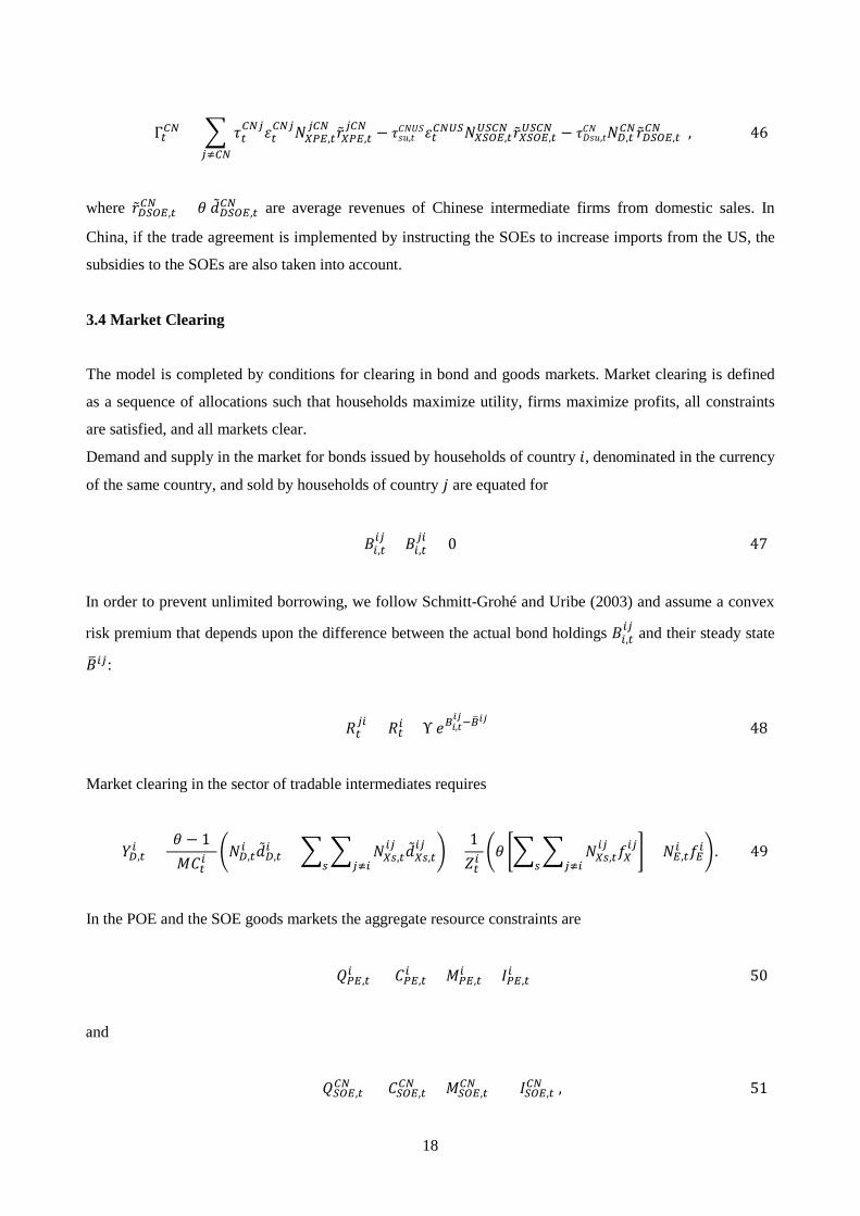
3.4 Market Clearing

The model is completed by conditions for clearing in bond and goods markets. Market clearing is defined

as a sequence of allocations such that households maximize utility, firms maximize profits, all constraints

are satisfied, and all markets clear.

Demand and supply in the market for bonds issued by households of country 𝑖, denominated in the currency

of the same country, and sold by households of country 𝑗 are equated for

𝐵𝑖,𝑡𝑖𝑖 + 𝐵𝑖,𝑡

𝑖𝑖 = 0 (47)

In order to prevent unlimited borrowing, we follow Schmitt-Grohé and Uribe (2003) and assume a convex

risk premium that depends upon the difference between the actual bond holdings 𝐵𝑖,𝑡𝑖𝑖 and their steady state

𝐵�𝑖𝑖:

𝑅𝑡𝑖𝑖 = 𝑅𝑡𝑖 + Υ 𝑒𝐼𝑖,𝑡

𝑖𝑗−𝐼�𝑖𝑗 (48)

Market clearing in the sector of tradable intermediates requires

𝑌𝐷,𝑡𝑖 =

(𝜃 − 1)𝑀𝐶𝑡𝑖

�𝐶𝐷,𝑡𝑖 �̃�𝐷,𝑡

𝑖 + � � 𝐶𝑋𝑖,𝑡𝑖𝑖 �̃�𝑋𝑖,𝑡

𝑖𝑖

𝑖≠𝑖𝑖�+

1𝑍𝑡𝑖

�𝜃 �� � 𝐶𝑋𝑖,𝑡𝑖𝑖 𝑓𝑋

𝑖𝑖

𝑖≠𝑖𝑖� + 𝐶𝑃,𝑡

𝑖 𝑓𝑃𝑖� . (49)

In the POE and the SOE goods markets the aggregate resource constraints are

𝑄𝑃𝑃,𝑡𝑖 = 𝐶𝑃𝑃,𝑡

𝑖 + 𝑀𝑃𝑃,𝑡𝑖 + 𝐼𝑃𝑃,𝑡

𝑖 (50)

and

𝑄𝑋𝑋𝑃,𝑡𝐶𝐶 = 𝐶𝑋𝑋𝑃,𝑡

𝐶𝐶 + 𝑀𝑋𝑋𝑃,𝑡𝐶𝐶 + +𝐼𝑋𝑋𝑃,𝑡

𝐶𝐶 , (51)

19

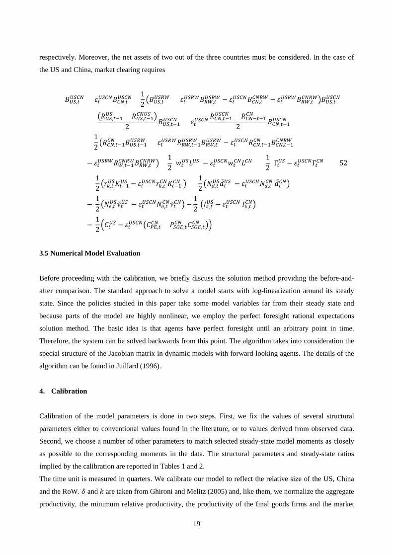
respectively. Moreover, the net assets of two out of the three countries must be considered. In the case of

the US and China, market clearing requires

𝐵𝐶𝑋,𝑡𝐶𝑋𝐶𝐶 + 𝜀𝑡𝐶𝑋𝐶𝐶𝐵𝐶𝐶,𝑡

𝐶𝑋𝐶𝐶 +12 �𝐵𝐶𝑋,𝑡𝐶𝑋𝐶𝐶 + 𝜀𝑡𝐶𝑋𝐶𝐶𝐵𝐶𝐶,𝑡

𝐶𝑋𝐶𝐶 − 𝜀𝑡𝐶𝑋𝐶𝐶𝐵𝐶𝐶,𝑡𝐶𝐶𝐶𝐶 − 𝜀𝑡𝐶𝑋𝐶𝐶𝐵𝐶𝐶,𝑡

𝐶𝐶𝐶𝐶�𝐵𝐶𝑋,𝑡𝐶𝑋𝐶𝐶

= �𝑅𝐶𝑋,𝑡−1

𝐶𝑋 + 𝑅𝐶𝑋,𝑡−1𝐶𝐶𝐶𝑋 �

2𝐵𝐶𝑋,𝑡−1𝐶𝑋𝐶𝐶 + 𝜀𝑡𝐶𝑋𝐶𝐶

𝑅𝐶𝐶,𝑡−1𝐶𝑋𝐶𝐶 + 𝑅𝐶𝐶−𝑡−1𝐶𝐶

2𝐵𝐶𝐶,𝑡−1𝐶𝑋𝐶𝐶

+12 �𝑅𝐶𝐶,𝑡−1𝐶𝐶 𝐵𝐶𝑋,𝑡−1

𝐶𝑋𝐶𝐶 + 𝜀𝑡𝐶𝑋𝐶𝐶𝑅𝐶𝐶,𝑡−1𝐶𝑋𝐶𝐶 𝐵𝐶𝐶,𝑡

𝐶𝑋𝐶𝐶 − 𝜀𝑡𝐶𝑋𝐶𝐶𝑅𝐶𝐶,𝑡−1𝐶𝐶 𝐵𝐶𝐶,𝑡−1

𝐶𝐶𝐶𝐶

− 𝜀𝑡𝐶𝑋𝐶𝐶𝑅𝐶,𝑡−1𝐶𝐶𝐶𝐶𝐵𝐶𝐶,𝑡

𝐶𝐶𝐶𝐶� +12

(𝑤𝑡𝐶𝑋𝐿𝐶𝑋 − 𝜀𝑡𝐶𝑋𝐶𝐶𝑤𝑡𝐶𝐶𝐿𝐶𝐶 ) +12

(Γ𝑡𝐶𝑋 − 𝜀𝑡𝐶𝑋𝐶𝐶Γ𝑡𝐶𝐶) (52)

+ 12 �𝑟𝑘,𝑡𝐶𝑋𝐾𝑡−1𝐶𝑋 − 𝜀𝑡𝐶𝑋𝐶𝐶𝑟𝑘,𝑡

𝐶𝐶𝐾𝑡−1𝐶𝐶 � + 12 �𝐶𝑑,𝑡𝐶𝑋�̃�𝑡𝐶𝑋 − 𝜀𝑡𝐶𝑋𝐶𝑈𝐶𝑑,𝑡

𝐶𝐶 �̃�𝑡𝐶𝐶�

− 12 �𝐶𝑒,𝑡𝐶𝑋𝜈�𝑡𝐶𝑋 − 𝜀𝑡𝐶𝑋𝐶𝐶𝐶𝑒,𝑡

𝐶𝐶𝜈�𝑡𝐶𝐶� −12

�𝐼𝑘,𝑡𝐶𝑋 − 𝜀𝑡𝐶𝑋𝐶𝐶 𝐼𝑘,𝑡

𝐶𝐶�

− 12�𝐶𝑡𝐶𝑋 − 𝜀𝑡𝐶𝑋𝐶𝐶�𝐶𝑃𝑃,𝑡

𝐶𝐶 + 𝑃𝑋𝑋𝑃,𝑡𝐶𝐶 𝐶𝑋𝑋𝑃,𝑡

𝐶𝐶 ��

3.5 Numerical Model Evaluation

Before proceeding with the calibration, we briefly discuss the solution method providing the before-and-

after comparison. The standard approach to solve a model starts with log-linearization around its steady

state. Since the policies studied in this paper take some model variables far from their steady state and

because parts of the model are highly nonlinear, we employ the perfect foresight rational expectations

solution method. The basic idea is that agents have perfect foresight until an arbitrary point in time.

Therefore, the system can be solved backwards from this point. The algorithm takes into consideration the

special structure of the Jacobian matrix in dynamic models with forward-looking agents. The details of the

algorithm can be found in Juillard (1996).

4. Calibration

Calibration of the model parameters is done in two steps. First, we fix the values of several structural

parameters either to conventional values found in the literature, or to values derived from observed data.

Second, we choose a number of other parameters to match selected steady-state model moments as closely

as possible to the corresponding moments in the data. The structural parameters and steady-state ratios

implied by the calibration are reported in Tables 1 and 2.

The time unit is measured in quarters. We calibrate our model to reflect the relative size of the US, China

and the RoW. 𝛿 and 𝑘 are taken from Ghironi and Melitz (2005) and, like them, we normalize the aggregate

productivity, the minimum relative productivity, the productivity of the final goods firms and the market

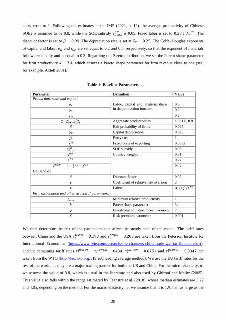
20

entry costs to 1. Following the estimates in the IMF (2021, p. 12), the average productivity of Chinese

SOEs is assumed to be 0.8, while the SOE subsidy 𝜏𝐷𝑖𝐷,𝑡𝐶𝐶 is 0.05. Fixed labor is set to 0.33 𝜉𝑖 𝜉𝐶𝑋⁄ . The

discount factor is set to 𝛽 = 0.99. The depreciation rate is set at 𝛿𝐾 = 0.25. The Cobb–Douglas exponents

of capital and labor, 𝜚𝐾 and 𝜚𝐿, are set equal to 0.2 and 0.5, respectively, so that the exponent of materials

follows residually and is equal to 0.3. Regarding the Pareto distribution, we set the Pareto shape parameter

for firm productivity 𝑘 = 3.4, which ensures a Pareto shape parameter for firm revenue close to one (see,

for example, Axtell 2001).

Table 1: Baseline Parameters

Parameter Definition Value Production, costs and capital

𝜚𝐿 Labor, capital and material share in the production function

0.5 𝜚𝐾 0.2 𝜚𝑀 0.3

𝑍𝑖 ,𝑍𝑃𝑃𝑖 ,𝑍𝑋𝑋𝑃𝐶𝐶 Aggregate productivities 1.0, 1.0, 0.8 𝛿 Exit probability of firms 0.025 𝛿𝐾 Capital depreciation 0.025 𝑓𝑃𝑖 Entry cost 1

𝑓𝑋𝑖𝑖 Fixed costs of exporting 0.0032

𝜏𝐷𝑖𝐷,𝑡𝐶𝐶 SOE subsidy 0.05 𝜉𝐶𝑋 Country weights 0.31 𝜉𝐶𝐶 0.27

𝜉𝐶𝐶𝐶 = 1 − 𝜉𝐶𝑋 − 𝜉𝐶𝐶 0.42 Households

𝛽 Discount factor 0.99 𝛾 Coefficient of relative risk aversion 2 𝐿 Labor 0.33 𝜉𝑖 𝜉𝐶𝑋⁄

Firm distribution and other structural parameters 𝑧𝑚𝑖𝑛 Minimum relative productivity 1 𝑘 Pareto shape parameter 3.4 𝜙 Investment adjustment cost parameter 7 Υ Risk premium parameter 0.001

We then determine the rest of the parameters that affect the steady state of the model. The tariff rates

between China and the USA 𝜏𝑡𝐶𝑋𝐶𝐶 = 0.193 and 𝜏𝑡𝐶𝐶𝐶𝑋 = 0.203 are taken from the Peterson Institute for

International Economics (https://www.piie.com/research/piie-charts/us-china-trade-war-tariffs-date-chart),

and the remaining tariff rates 𝜏𝑡𝐶𝐶𝐶𝐶𝑋 = 𝜏𝑡𝐶𝐶𝐶𝐶𝐶 = 0434, 𝜏𝑡𝐶𝐶𝐶𝐶𝐶 = 0.0751 and 𝜏𝑡𝐶𝑋𝐶𝐶𝐶 = 0.0347 are

taken from the WTO (http://tao.wto.org, HS subheading average method). We use the EU tariff rates for the

rest of the world, as they are a major trading partner for both the US and China. For the micro-elasticity, 𝜃,

we assume the value of 3.8, which is usual in the literature and also used by Ghironi and Melitz (2005).

This value also falls within the range estimated by Feenstra et al. (2018), whose median estimates are 3.22

and 4.05, depending on the method. For the macro elasticity, 𝜔, we assume that it is 1.9, half as large as the

21

micro elasticity, the so-called rule of two. Furthermore, we use country weightings, 𝜉𝑖, the degree of

openness, 𝛼𝑖, as well as the iceberg trade costs, 𝜏𝐼𝐼𝑖𝑖 , to match key trade figures. Moreover, the fixed costs of

exporting are calibrated such that somewhat more than 21 percent of firms export to match the US ratio of

exporters reported by Bernard et al. (2003). Steady-state bond holdings are calibrated according to the net

international investment position reported by the IMF (https://data.imf.org/regular.aspx?key=62805745). In

accordance with this, the US has a net debt of 51.6 percent of its GDP, while China has net claims

amounting to 14.8 percent of its GDP. For the sake of simplicity, we assume that China has only claims on

the US. Furthermore, we assume that 80 percent of the debt is denominated in US dollars. Given these

parameter values, we solve for the open-economy equilibrium of the heterogeneous firm model. The results

are given in Table 2.

Table 2: Selected Steady-State Ratios Implied by the Baseline Calibration

(The actual ratios are given in parentheses)

Ratio US China RoW

GDP as ratio of world GDP 24.4 (24.4) 16.3 (16.3) 59.3 (59.3)

Trade as ratio of GDP 27.2 (26.4) 35.1 (35.7) 18.11

US–China-trade as ratio of overall US trade 12.0 (11.3) --- ---

Ratio of US imports from China to exports to China 2.8 (2.9) ---

Ratio of exporting firms 24.4 23.5 7.4

Output of state-owned enterprises to GDP --- 26.5 (23–28) ---

Notes: The model GDP ratio of country 𝑖 is defined by GDP𝑖 �GDP𝑖 + ∑ 𝜀𝑖𝑖𝐺𝐷𝑃𝑖𝑖≠𝑖 �� , the actual numbers are taken from the World Bank and the US Census Bureau. The model values can be obtained by 𝛼𝐶𝑋 = 0.2117,𝛼𝐶𝐶 =0.2699,𝛼𝑃𝐶 = 0.1180, 𝜅𝑖𝑖 = GDP𝑖/∑ GDP𝑖𝑖≠𝑖 , where GDP refers to the actual and not the model value. The iceberg trade costs are assumed to be 𝜏𝐼𝐼,𝑡

𝐶𝑋𝐶𝐶 = 2.3, 𝜏𝐼𝐼,𝑡𝐶𝑋𝐶𝐶𝐶 = 1.4, 𝜏𝐼𝐼,𝑡

𝐶𝐶𝐶𝑋 = 1.5, 𝜏𝐼𝐼,𝑡𝐶𝐶𝐶𝐶𝑋 = 1.7, 𝜏𝐼𝐼,𝑡

𝐶𝐶𝐶𝐶𝐶 = 1.3 and 𝜏𝐼𝐼,𝑡𝐶𝐶𝐶𝐶𝐶 =

1.5. Fixed costs of exporting are set to 𝑓𝑋𝑖𝑖 = 0.0032. Following Zhang (2019), the SOE weight in the model is

1 − 𝜒 = 0.31. Steady-state bond holdings are assumed to be 𝐵�𝐶𝑋,𝑡𝐶𝐶𝐶𝑋 = 0.2240, 𝐵�𝐶𝐶,𝑡

𝐶𝐶𝐶𝑋 = 0.0560, 𝐵�𝐶𝑋,𝑡𝐶𝐶𝐶𝐶𝑋 = 2.3360,

𝐵�𝐶𝐶𝐶,𝑡𝐶𝐶𝐶𝐶𝑋 = 0.5840 and 𝐵�𝐶𝐶,𝑡

𝐶𝐶𝐶𝐶𝐶 = 𝐵�𝐶𝐶𝐶,𝑡𝐶𝐶𝐶𝐶𝐶 = 0.

5. Model Dynamics

The modelling framework provides a rich laboratory for the analysis of trade policies. Below we explore

numerically the properties of the model. In doing so we cast a special focus on facilitating trade through the

phase one agreement. We also conduct various policy experiments.

5.1 Quantifying the Trade and Income Effects of the Phase One Deal

In simulating the impact of the asymmetric trade agreement, an assumption must be made about its

implementation by the Chinese government. In particular, an assumption must be made about the

22

underlying transmission process leading to the surge in imports. Furthermore, different assumptions can

also be made about the degree of compliance with the contractual voluntary import expansions (VIEs).

As per the text of the agreement, Chinese imports of goods and services from the US are supposed to

increase by 41 percent in 2020 and even by 66 percent in 2021 compared to the trade deal benchmark year

2017. 16 When compared to the lower imports in 2019, this even amounts to increases of 47 percent and 75

percent in 2020 and 2021, respectively. The trade agreement does not specify how the targets should be met

by China. In what follows, we therefore present model simulations for four different policy scenarios

regarding the actual implementation of the phase one trade deal.17

First, the Chinese government “guides” the SOEs to increase imports from the US.18 More precisely, the

government commits the SOE sector to increase its share of imports from the US by 162 percent in 2020

and once again by 98 percent in 2021 compared to the steady state calibrated for 2019. These quantitative

targets would just imply a complete fulfillment of the contractual obligations. This relative minimum

demand, referred to in the literature as market share VIE (Greaney 1996; 1999), increases the SOEs’

marginal costs and thus their product prices. After weighting with the SOEs’ importance and general

equilibrium knock-on effects, this results in overall import adjustments.

Second, the Chinese government again implements the required increase in imports by means of the SOEs.

Notwithstanding the contractual agreement, however, this time only by up to 65 percent. This corresponds

to the current achievement level. In quantitative terms, this corresponds to an increase of total US exports to

China by 15 percent in 2020 and by 29 percent in 2021 compared to 2019. To achieve this increase in total

imports SOE imports from the US have to increase by 54 percent in 2020 and once again by 47 percent in

2021. In the simulations, it is assumed that tariff rates remain unchanged even if the additional SOE imports

cannot fully meet the contractual obligations.

In the third scenario, the import increase is again by means of the SOEs and the degree of contract

fulfillment is again 65 percent. In contrast to the previous scenarios, however, the SOE imports from the

USA are subsidized by the government. The needed subsidy for the 65 percent fulfillment of the deal is 14

percent in the first year and 23 percent in the second year.

Finally, we consider the case that China fulfills the trade agreement by means of a unilateral import tariff

cut to 7.51 percentage points for US imports. This hypothetical import tariff rate corresponds to the current

most-favored-nation tariff rate, which also applies to RoW countries. In other words, China meets the VIE

import targets from the US by means of a nondiscriminatory reduction of import tariffs rather than through

a preferential access of US producers to the Chinese market. The nondiscriminatory tariff reduction to this 16 The outcome-based phase one trade agreement looks more like a ceasefire than a resolution of the US–China trade conflict. But there are also geopolitical considerations and strategic imperatives that have led to a critical bipartisan sentiment towards China in the US Congress. Since it is unclear whether this resentment threatening the world trade architecture is only temporary or is instead secular, the trade deal is assumed to be permanent in the numerical simulations and thus the import commitments for 2021 continue to apply. 17 The aggregate effects mask heterogeneous impacts across product groups. How will the Chinese extra imports be distributed across products? For an analysis of the distribution of extra purchases across the top-ten products, taking into account the US production constraints, see Cerutti et al. (2019) and the IMF (2019, p. 54). 18 “Guiding” is a widely used policy tool in China. For a theoretical modeling analysis of this approach in a different context, see Chen et al. (2020).

23

extent achieves about the same gains in US exports to China as targeted under the agreement for the year

2020. In the subsequent year 2021, this reduced tariff rate will be adhered to, although the import

obligations from the US will not be fully met.

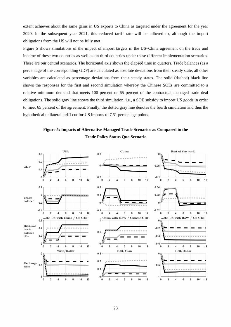
Figure 5 shows simulations of the impact of import targets in the US–China agreement on the trade and

income of these two countries as well as on third countries under these different implementation scenarios.

These are our central scenarios. The horizontal axis shows the elapsed time in quarters. Trade balances (as a

percentage of the corresponding GDP) are calculated as absolute deviations from their steady state, all other

variables are calculated as percentage deviations from their steady states. The solid (dashed) black line

shows the responses for the first and second simulation whereby the Chinese SOEs are committed to a

relative minimum demand that meets 100 percent or 65 percent of the contractual managed trade deal

obligations. The solid gray line shows the third simulation, i.e., a SOE subsidy to import US goods in order

to meet 65 percent of the agreement. Finally, the dotted gray line denotes the fourth simulation and thus the

hypothetical unilateral tariff cut for US imports to 7.51 percentage points.

Figure 5: Impacts of Alternative Managed Trade Scenarios as Compared to the

Trade Policy Status Quo Scenario

24

The first impression is that the implications of the agreement depend on how China implements it. For the

US, there is an increase in GDP in all four scenarios. As expected, the discriminatory VIE with 100 percent

compliance (black solid line) leads to the largest effect. In this case, the GDP increase amounts to 0.17

percent in the first year and 0.25 percent in the second year. This magnitude is comparable to other

estimates in the literature. Examples include the size of the export demand shock impact as examined in

Backus et al. (1992) based on the International Real Business Cycle model or Lubik and Schorfheide

(2005) based on the two-country New Open Economy Macroeconomics model.19

In the remaining three scenarios the GDP increase is smaller due to the merely 65 percent compliance, but

still positive. The four policy scenarios deliver different effects on Chinese GDP. Marked effects arise

above all in the first and fourth scenarios. The first scenario with 100% contract fulfillment via VIE leads to

a persistent GDP loss. In the other three scenarios, the exchange rate depreciation against the US dollar

plays a role. In particular, the unilateral tariff reduction and subsequent devaluation of the Chinese currency

results in an expansionary effect due to China’s increased price competitiveness in both foreign

countries/markets.

What are the associated impacts for China? The impact on China’s welfare is negative if the market is

under free trade and ambiguous in the case of products in protected industries. The ambiguity for China

depends on the fact that increased imports from the US may drive out less efficient Chinese producers or

more efficient producers from the RoW. This efficiency gain is particularly evident in the case of the

across-the-board tariff reduction to the most-favored-nation rate. A follow-up set of effects may result from

the distortions created by the VIE in China. Chinese producers, seeing the domestic price decline, may sell

part of their production abroad. This form of trade deflection will have negative consequences for producers

in the RoW, which will suffer from the increased competition from Chinese exporters, and a positive effect

on RoW consumers who will benefit from lower prices.20

Moreover, in the RoW countries there is a negative GDP impact, which is a mirror image of that in the US.

The underlying mechanism is again clear. The trade deal incentivizes China to shift imports away from

other suppliers and towards the US and thus leads to international trade diversion. In political terms: the

discriminatory trade agreement follows a nationalist, not a globalist approach.21

Last but not least, the temporary trade balance effects result from consumption smoothing of forward-

looking agents with assumed perfect foresight of the lasting nature of the trade deal. Beyond these

19 In contrast, qualitatively equivalent but quantitatively larger effects are found in the dynamic computable general equilibrium (CGE) modeling framework in Freund et al. (2020). Each country contains multiple sectors linked through an input–output structure to other domestic and foreign sectors. In this setup, a tariff introduces an inefficiency in the allocation of resources across sectors. Unlike CGE, there is limited sectoral disaggregation in the open-economy macro model. On the other hand, emphasis is on dynamics, stock-flow consistency, and forward-looking expectations. As a result, both approaches highlight different implications of the distortions brought about by trade policies. 20 This mechanism has been referred to as trade deflection by Bown and Crowley (2007) in the context of US anti-dumping duties against Japan. 21 Our results complement other studies. Model-based analyses have found noticeable spillover effects for countries not directly affected by protectionist policies in relation to the trade conflict between the US and China. See, for example, Bolt et al. (2019) and the IMF (2018, pp. 33–35). The evidence of significant trade diversion effects is also consistent with the IMF’s (2019, pp. 51–59) empirical analyses. The IMF estimates based on granular trade data reveal a substantial “exports-at-risk” for the EU, Japan and Korea.

25

temporary effects, there is a permanent improvement in the US–China bilateral trade balance, but no lasting

improvement in the overall US trade balance.

5.2 Future US–China Trade Agreements: Some Policy Experiments

Much of the current trade policy debate, in the US as well as internationally, revolves around the future US

trade policy. This applies in particular with respect to the policy towards China.22 The broad bipartisan

consensus in the US comprises the belief of the need to stand up to China. Democrats and Republicans now

see China as a strategic adversary, so it is not likely that President Biden will turn the clock back past

Trump’s and restore the old policy of engagement.23 Signs are already emerging that elements of the Trump

approach will remain in place. That augurs poorly for a quick end to the trade war. But when a simple

“reset” in trade relations is unlikely to happen, what might a future trade agreement look like?

In recent years the US trade policy has become a muddle of tariffs, VIE deals, and ad hoc bans. President

Biden has committed himself to developing a more coherent and effective strategy. Moreover, he has

declared that he will use a broader range of tools than in the phase one deal. Such a broader policy approach

may include further structural issues in particular. One concern about China is a set of structural policies

that are outside the norms of advanced economies: extensive nontariff barriers, restrictions on foreign

investment in some sectors, limited intellectual property right protection, forced technology transfers, and

subsidies to SOEs. This raises the question, what will the new US government do with the tariffs and VIEs?

Strategy might play a role: the Biden administration may be willing to negotiate away some of the VIEs and

import tariffs in exchange for a phase two agreement that addresses some of these structural concerns.

Having a model suited to study trade deals, we perform several policy experiments in the next step. In other

words, we think outside the phase one box. Whether and how soon the Biden administration will

renegotiate the phase one trade deal, and what it will seek in return, is currently an open question. Although

the current deal is far from a reset, and negotiations will be thorny, we would like to take a look at a

conceivable mutually beneficial future phase two deal.

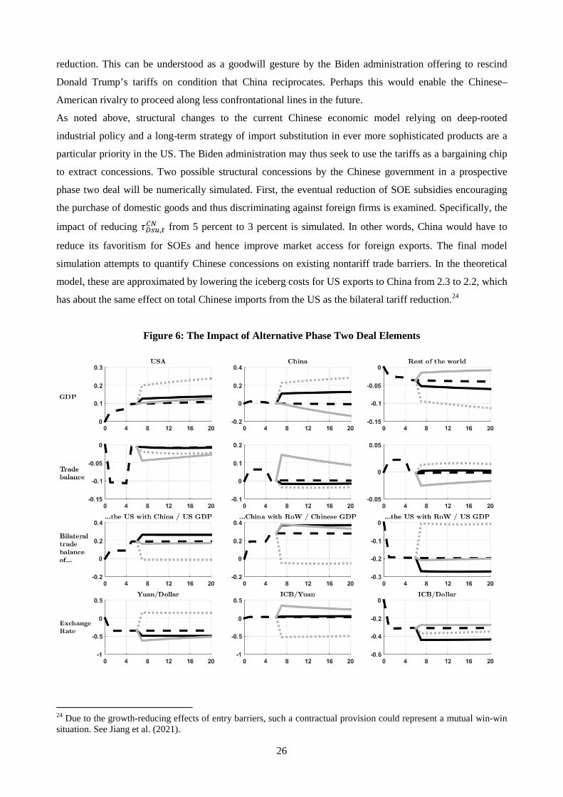
In our simulations, we assume that a possible phase two deal takes effect in the seventh quarter after the

start of the implementation of the phase one deal and is not anticipated by the households. In Figure 6 the

isolated effects of four possible renegotiated contract provisions are simulated.

First, since China has not yet met the quantitative targets in the phase one deal in full, the follow-up phase

two deal could set the lower level of fulfillment achieved so far as a new target. In other words, the 65

percent Chinese VIE surge from the US achieved to date is assumed to be the new phase two contractual

import requirement. Second, the two parties agree on a mutual 5 percentage point bilateral import tariff 22 Given the recent signing of the so-called Regional Comprehensive Economic Partnership (RCEP) free-trade agreement amongst 15 Asian countries that will create the world’s largest regional free-trade zone, the future US trade agenda will naturally gravitate towards Asia. 23 What complicates the matter further is the fact that China’s political openness has reversed trajectory under President Xi Jinping. Therefore, decoupling in high-tech areas may remain the trend. The “Made in China 2025” program, the new Chinese economic catchphrase “dual circulation,” and the pointer to the necessity of self-sufficiency in key technologies reveals that the Chinese government also expects such a scenario.

26

reduction. This can be understood as a goodwill gesture by the Biden administration offering to rescind

Donald Trump’s tariffs on condition that China reciprocates. Perhaps this would enable the Chinese–

American rivalry to proceed along less confrontational lines in the future.

As noted above, structural changes to the current Chinese economic model relying on deep-rooted

industrial policy and a long-term strategy of import substitution in ever more sophisticated products are a

particular priority in the US. The Biden administration may thus seek to use the tariffs as a bargaining chip

to extract concessions. Two possible structural concessions by the Chinese government in a prospective

phase two deal will be numerically simulated. First, the eventual reduction of SOE subsidies encouraging

the purchase of domestic goods and thus discriminating against foreign firms is examined. Specifically, the

impact of reducing 𝜏𝐷𝑖𝐷,𝑡𝐶𝐶 from 5 percent to 3 percent is simulated. In other words, China would have to

reduce its favoritism for SOEs and hence improve market access for foreign exports. The final model

simulation attempts to quantify Chinese concessions on existing nontariff trade barriers. In the theoretical

model, these are approximated by lowering the iceberg costs for US exports to China from 2.3 to 2.2, which

has about the same effect on total Chinese imports from the US as the bilateral tariff reduction.24

Figure 6: The Impact of Alternative Phase Two Deal Elements

24 Due to the growth-reducing effects of entry barriers, such a contractual provision could represent a mutual win-win situation. See Jiang et al. (2021).

27

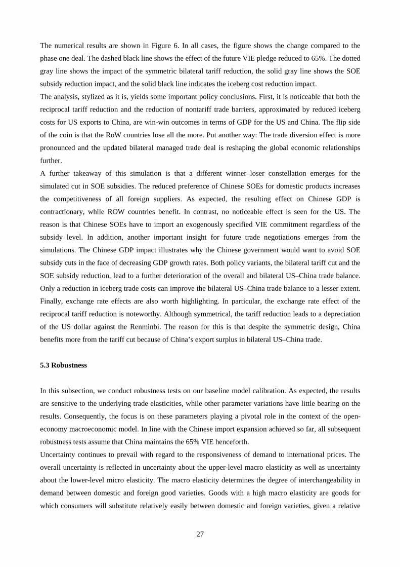
The numerical results are shown in Figure 6. In all cases, the figure shows the change compared to the

phase one deal. The dashed black line shows the effect of the future VIE pledge reduced to 65%. The dotted

gray line shows the impact of the symmetric bilateral tariff reduction, the solid gray line shows the SOE

subsidy reduction impact, and the solid black line indicates the iceberg cost reduction impact.

The analysis, stylized as it is, yields some important policy conclusions. First, it is noticeable that both the

reciprocal tariff reduction and the reduction of nontariff trade barriers, approximated by reduced iceberg

costs for US exports to China, are win-win outcomes in terms of GDP for the US and China. The flip side

of the coin is that the RoW countries lose all the more. Put another way: The trade diversion effect is more

pronounced and the updated bilateral managed trade deal is reshaping the global economic relationships

further.

A further takeaway of this simulation is that a different winner–loser constellation emerges for the

simulated cut in SOE subsidies. The reduced preference of Chinese SOEs for domestic products increases

the competitiveness of all foreign suppliers. As expected, the resulting effect on Chinese GDP is

contractionary, while ROW countries benefit. In contrast, no noticeable effect is seen for the US. The

reason is that Chinese SOEs have to import an exogenously specified VIE commitment regardless of the

subsidy level. In addition, another important insight for future trade negotiations emerges from the

simulations. The Chinese GDP impact illustrates why the Chinese government would want to avoid SOE

subsidy cuts in the face of decreasing GDP growth rates. Both policy variants, the bilateral tariff cut and the

SOE subsidy reduction, lead to a further deterioration of the overall and bilateral US–China trade balance.

Only a reduction in iceberg trade costs can improve the bilateral US–China trade balance to a lesser extent.

Finally, exchange rate effects are also worth highlighting. In particular, the exchange rate effect of the

reciprocal tariff reduction is noteworthy. Although symmetrical, the tariff reduction leads to a depreciation

of the US dollar against the Renminbi. The reason for this is that despite the symmetric design, China

benefits more from the tariff cut because of China’s export surplus in bilateral US–China trade.

5.3 Robustness

In this subsection, we conduct robustness tests on our baseline model calibration. As expected, the results

are sensitive to the underlying trade elasticities, while other parameter variations have little bearing on the

results. Consequently, the focus is on these parameters playing a pivotal role in the context of the open-

economy macroeconomic model. In line with the Chinese import expansion achieved so far, all subsequent

robustness tests assume that China maintains the 65% VIE henceforth.

Uncertainty continues to prevail with regard to the responsiveness of demand to international prices. The

overall uncertainty is reflected in uncertainty about the upper-level macro elasticity as well as uncertainty

about the lower-level micro elasticity. The macro elasticity determines the degree of interchangeability in

demand between domestic and foreign good varieties. Goods with a high macro elasticity are goods for

which consumers will substitute relatively easily between domestic and foreign varieties, given a relative

28

change in domestic and foreign prices. On the other hand, goods with a low macro elasticity imply that

consumers stay with their preferred variety more firmly and are less willing to substitute between the two.

The micro elasticity reflects the second-tier choices between suppliers of the imported good at the country

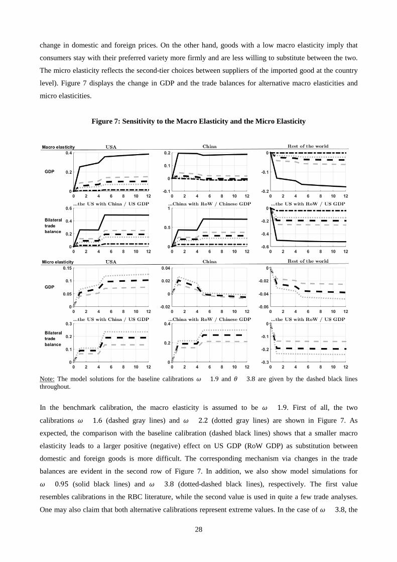
level). Figure 7 displays the change in GDP and the trade balances for alternative macro elasticities and

micro elasticities.

Figure 7: Sensitivity to the Macro Elasticity and the Micro Elasticity

Note: The model solutions for the baseline calibrations 𝜔 = 1.9 and 𝜃 = 3.8 are given by the dashed black lines throughout.

In the benchmark calibration, the macro elasticity is assumed to be 𝜔 = 1.9. First of all, the two

calibrations 𝜔 = 1.6 (dashed gray lines) and 𝜔 = 2.2 (dotted gray lines) are shown in Figure 7. As

expected, the comparison with the baseline calibration (dashed black lines) shows that a smaller macro

elasticity leads to a larger positive (negative) effect on US GDP (RoW GDP) as substitution between

domestic and foreign goods is more difficult. The corresponding mechanism via changes in the trade

balances are evident in the second row of Figure 7. In addition, we also show model simulations for

𝜔 = 0.95 (solid black lines) and 𝜔 = 3.8 (dotted-dashed black lines), respectively. The first value

resembles calibrations in the RBC literature, while the second value is used in quite a few trade analyses.

One may also claim that both alternative calibrations represent extreme values. In the case of 𝜔 = 3.8, the

29

impact on US GDP decreases to almost zero, while the GDP effect for 𝜔 = 0.95 increases to 0.36 in the

second year. For 𝜔 = 0.95, the interesting finding is that China’s GDP is also rising. In other words, the

low macro elasticity leads to internationally correlated business cycles.25 Again the trade response is

decreasing in the macro elasticity of substitution.

For the micro elasticity, alternative model solutions for 𝜃 = 3.4 (dashed gray lines) and 𝜃 = 4.2 (dotted

gray lines) are given in Figure 7. The baseline calibration is 𝜃 = 3.8 (dashed black lines). As can be seen,

the higher the micro elasticity, the greater the positive effect on US GDP and the negative trade diversion

effect upon the RoW GDP. By way of comparison, the results for China are quite robust with respect to the

changes in the micro elasticity.

6. Welfare

In this section we briefly touch upon welfare. Following Schmitt-Grohé and Uribe (2007), the welfare

effects of the phase one agreement and hypothetical phase two agreements are calculated relative to a

reference policy scenario. In case of the phase one agreement, the reference policy scenario is the

continuation of the status quo of 2019 (equal to the model steady state). In the case of eventual phase

agreements, we take the continuation of the 65% market share VIE as the reference policy scenario.

Throughout, the welfare difference is expressed as the percentage of consumption that households are

willing to give up in order to be as well off under the corresponding trade policy as under the reference

policy. Given the representative household’s objective function, the consumption-equivalent welfare gain is

given by:

Welfare Gain = �𝑉0𝑎

𝑉0𝑟�

11−𝛾

− 1 , (53)

where 𝑉0𝑎 is the welfare of the respective policy alternative, and 𝑉0𝑟 is the welfare of the respective

reference policy. The net present value of utility is thereby calculated according to equation (34). The

results are given in Table 3.

Three results should be highlighted from the multitude of findings. First, the welfare effects for the US are

positive across the board. However, the magnitude of the welfare effects depends – as expected – on the

extent of managed trade achieved. Second, China’s welfare would decline in the event of full compliance

with the phase one agreement. Likewise, a reduction in SOE subsidies in a potential phase two agreement

would lead to a negative welfare effect. Finally, the trade diversion effects lead to negative welfare effects

for the RoW countries, the magnitude of which depends on the degree of implementation of the phase one

agreement.

25 That is why such an elasticity is typically used in the international RBC literature. See, e.g., Heathcote and Perri (2002).

30

Table 3: Welfare Analysis

USA China Rest of the World

Welfare gains and losses of the phase one agreement compared to a continuation of the status quo at the end of 2019

100% market share VIE 0.30 -0.13 -0.10

65% market share VIE 0.12 0.01 -0.04

SOE import subsidy to reach 65% fulfillment 0.24 0.13 -0.09

Unilateral tariff reduction 0.17 0.02 -0.06

Welfare gains and losses of potential phase two agreement elements compared to only a continuation of the 65%

market share VIE

5% bilateral import tariff reduction 0.15 0.33 -0.08

Reduced SOE subsidies 0.01 -0.22 0.02

Reduction of Chinese nontariff trade barriers with the US 0.04 0.17 -0.02

7. Conclusions

The racking up of US–China trade disputes and the shift away from a multilateral, rules-based trading

system has led to a growing interest in quantifying the effects of protectionist trade policies. Besides

assessing the impacts of Donald Trump’s trade policy modus operandi on the US economy, both

researchers and policymakers are also interested in the effects on third countries. Against this background,

we study the consequences of managed trade policies through the lens of a formal model. In a nutshell, the

paper considers a new open-economy macroeconomics model split between three large trading partners, the

United States, China, and the rest of the world. We have illustrated noticeable positive (negative) of the

agreement for the United States (China) as well as negative spillover effects for countries not directly

affected by the managed trade deal due to trade diversion. An important by-product of our approach is that

it can be used to provide quantitative evaluations of potential future trade agreements. To the best of our

knowledge, we are the first to analyze the phase one Sino–American managed trade agreement in such a

state-of-the-art modeling framework.

We invite the reader to cautiously interpret our results, with some caveats that should be kept in mind. In

particular, the work presented in this paper could be expanded in three ways. One impact not accounted for

in the model is the COVID-19 pandemic. The pandemic may leave a lasting imprint on the world economy

that goes beyond a short-term recession, causing changes away from global just-in-time supply chains. This

is reinforced by the growth of nationalism and “my nation first” policies pushing firms to reshore some of

their production in favor of national and regional supply chains. The disruption caused by the COVID-19

pandemic is amplifying this trend by undermining confidence in international supply chains.26 Furthermore,

26The business magazine The Economist has referred to this process as “slowbalisation”. See https://www.economist.com/leaders/2019/01/24/the-steam-has-gone-out-of-globalisation. Antras (2020) offers some

31

unresolved US–China trade policy disputes create uncertainty about the future. The knock-on effects of this

uncertainty on strategic company decisions dampening global economic growth have likewise not been

considered in the model.27 Finally, the fragmentation of production across borders has changed the nature

of trade, resulting in an increasing importance of trade in value added rather than traditional trade. One

implication, among others, is that the standard notion of the competitiveness effect of exchange rate

changes is no longer valid because exchange rate changes no longer have only the standard effect on trade

of making purely domestically (foreign) produced goods cheaper (or more expensive) for foreigners

(nationals).28 Further research on these aspects will provide a better understanding of the effects of trade

disputes.

thoughts worth reading on hyperglobalisation running out of steam and the future of global value chains in the post COVID-19 world. 27 See Caldara et al. (2020) and Handley and Limão (2017). 28 Bems and Johnson (2017) have made an important contribution to our understanding of this phenomenon.

32

References: Amiti, M., Redding, S.J. and Weinstein, D. (2019), “The impact of the 2018 Trade War on U.S. prices and welfare”, Journal of Economic Perspectives, 33, 187–210. Antras, P. (2020), “De-Globalisation? Global Value Chains in the Post-COVID-19 Age”, NBER Working Paper No. 28115, Cambridge (Mass.). Autor, D.H., Dorn, D., Hanson, G.H. and Majlesi, K. (2020), “Importing political polarization? The electoral consequences of rising trade exposure”, American Economic Review, 110, 3139–3183. Axtell, R.L. (2001), “Zipf distribution of US firm sizes”, Science, 293, 1818–1820. Backus, D., Kehoe, P.J. and Kydland, F.E. (1992), “International real business cycles”, Journal of Political Economy, 100, 745–775. Bagwell, K. and Staiger, R.W. (1990), “A theory of managed trade”, American Economic Review, 80, 779–795. Bems, R., and Johnson, R.C. (2017), “Demand for value added and value-added exchange rates”, American Economic Journal: Macroeconomics 9, 45-90. Bernard, A.B., Eaton, J., Jensen, J.B. and Kortum, S. (2003), “Plants and productivity in international trade”, American Economic Review, 93, 1268–1290. Bhagwati, J. (1987), “VERs, Quid pro quo DFI, and VIEs: Political–economy theoretic analyses”, International Economic Journal, 1, 1–14. Bjorksten, N. (1994), “Voluntary import expansions and voluntary export restraints in an oligopoly model with capacity constraints”, Canadian Journal of Economics, 27, 446–457. Bolt, W., Mavromatis, K. and van Wijnbergen, S. (2019), “The global macroeconomics of a trade war: The EAGLE model on the US–China trade conflict”, De Nederlandsche Bank Working Paper No. 623, Amsterdam. Bown, C.P. and Crowley, M.A. (2007), “Trade deflection and trade depression”, Journal of International Economics, 72, 176–201. Caldara, D., Iacoviello, M., Molligo, P., Prestipino, A. and Raffo, A. (2020), “The economic effects of trade policy uncertainty”, Journal of Monetary Economics, 109, 38–59. Caliendo, L., Feenstra, R.C., Romalis, J. and Taylor, A.M. (2015), “Tariff reductions, entry, and welfare: Theory and evidence for the last two decades”, NBER Working Paper No. 21768, Cambridge (Mass.). Cerutti, E.M., Chen, S., Deb, P., Gjonbalaj, A., Hannan, S.A. and Mohommad, A. (2019), “Managed trade: What could be possible spillover effects of a potential trade agreement between the U.S. and China?”, IMF Working Paper No. 19/251, Washington. Chen, H., Funke, M., Lozev, I. and Tsang, A. (2020), “To guide or not to guide? Quantitative monetary policy tools and macroeconomic dynamics in China”, International Journal of Central Banking, 16, 49–94. Chowdhry, S. and. Felbermayr, G. (2020a), “The US–China trade deal: How the EU and WTO lose from managed trade”, Kiel Institute for the World Economy Policy Brief No. 132, Kiel. Chowdhry, S. and Felbermayr, G. (2020b), “The US–China trade deal and its impact on China’s key trading partners”, Kiel Institute for the World Economy Policy Brief No. 134, Kiel.

33

Colantone, I. and Stanig, P. (2018a), “The trade origins of economic nationalism: Import competition and voting behavior in Western Europe”, American Journal of Political Science, 62, 936–953. Colantone, I. and Stanig, P. (2018b), “Global competition and Brexit”, American Political Science Review, 112, 201–218. Dinopoulos, E. and Kreinin, M.E. (1990), “An economic analysis of trade expansion policies”, Economic Inquiry, 28, 99–108. Ethier, W. and Horn, H. (1996), “Results-oriented trade policy”, Review of International Economics, 4, 17–39. Fajgelbaum, P.D., Goldberg, P.K., Kennedy, P.J. and Khandelwal, A.K. (2020), “The return to protectionism”, The Quarterly Journal of Economics, 135, 1–55. Feenstra, R.C., Luck, P., Obstfeld, M. and Russ, K.N. (2018), “In search of the Armington elasticity”, Review of Economics and Statistics, 100, 135–150. Freund, C, Maliszewska, M., Mattoo A. and Ruta, M. (2020), “When elephants make peace: The impact of the China–U.S. trade agreement on developing countries”, World Bank Policy Research Working Paper No. 9173, Washington DC. Ghironi, F. and Melitz, M.J. (2005), “International trade and macroeconomic dynamics with heterogeneous firms”, The Quarterly Journal of Economics, 120, 865–915. Greaney, T. (1996), “Import now! An analysis of market-share voluntary import expansions (VIEs)”, Journal of International Economics, 40, 149–163. Greaney, T. (1999), “Manipulating market shares: The indirect effects of voluntary import expansions”, Japan and the World Economy, 11, 96–113. Grossman, G. and Helpman, E. (1994), “Protection for sale”, American Economic Review, 84, 833–850. Handley, K., and Limão, N. (2017), “Policy uncertainty, trade, and welfare: Theory and evidence for China and the United States”, American Economic Review, 107, 2731–2783. Handley, K., Kamal, F. and Monarch, R. (2020), “Rising import tariffs, falling export growth: When modern supply chains meet old-style protectionism”, NBER Working Paper No. 26611, Washington DC. Heathcote, J. and Perri, F. (2002), “Financial autarky and international business cycles”, Journal of Monetary Economics, 49, 601–627. Hopenhayn, H. (1992), “Entry, exit, and firm dynamics in long run equilibrium”, Econometrica, 60, 1127–1150. IMF (2018), “World Economic Outlook”, October, Washington DC. IMF (2019), “People’s Republic of China – Selected Issues”, IMF Country Report No. 19/274, Washington DC. IMF (2021), “People’s Republic of China – Selected Issues”, IMF Country Report No. 21/12, Washington DC. Jiang, H., Zheng, Y. and Lijun, Z. (2021), “Growing through competition: The reduction of entry barriers among Chinese manufacturing firms”, CEPR Discussion Paper No. 15763, London.

34

Juillard, M. (1996), “Dynare: A program for the resolution and simulation of dynamic models with forward variables through the use of a relaxation algorithm”, CEPREMAP Working Paper No. 9602, Paris. Krugman P.R. (1980), “Scale economies, product differentiation, and the pattern of trade”, American Economic Review, 70, 950–959. Lubik, T.A. and Schorfheide, F. (2005), “A Bayesian look at new open economy macroeconomics”, In: Gertler, M. and Rogoff, K. (Eds) NBER Macroeconomics Annual 2005, Cambridge (MIT Press), 313–365. Mattoo, A., Mulabdic, A. and Ruta, M. (2020), “Trade creation and trade diversion in deep agreements”, Worldbank Policy Research Working Paper No. 8206, Washington DC. Melitz, M.J. (2003), “The impact of trade on intra‐industry reallocations and aggregate industry productivity”, Econometrica, 71, 1695–1725. Redding, S.J. (2011), “Theories of heterogeneous firms and trade”, Annual Review of Economics, 3, 77–105. Rodrik, D. (2018), “What do trade agreements really do?”, Journal of Economic Perspectives, 23, 73–90. Schmitt-Grohé, S. and Uribe, M. (2003), “Closing small open economy models”, Journal of International Economics, 61, 163–185. Schmitt-Grohé, S. and Uribe, M. (2007), “Optimal simple and implementable monetary and fiscal rules”, Journal of Monetary Economics, 54, 1702–1725. Zhang, C. (2019), How Much Do State-Owned Enterprises Contribute to China’s GDP and Employment? World Bank, Washington DC.