Embed Size (px)
Citation preview
This PDF is a selection from an out-of-print volume from the National Bureauof Economic Research
Volume Title: Developing Country Debt and Economic Performance, Volume1: The International Financial System
Volume Author/Editor: Jeffrey D. Sachs, editor
Volume Publisher: University of Chicago Press
Volume ISBN: 0-226-73332-7
Volume URL: http://www.nber.org/books/sach89-1
Conference Date: September 21-23, 1987
Publication Date: 1989
Chapter Title: The U.S. Capital Market and Foreign Lending, 1920–1955
Chapter Author: Barry Eichengreen
Chapter URL: http://www.nber.org/chapters/c8988
Chapter pages in book: (p. 107 - 156)
3 The U.S. Capital Market and Foreign Lending, 1920 - 1955 Barry Eichengreen
3.1 Introduction
In happier times (the 1970s), countries were thought to pass through stages of indebtedness analogous to the stages of the international product cycle. According to the stages theory (e.g., de Vries 1971), countries in the initial phases of the process (before “takeoff into in- debtedness”) lack the political stability and economic infrastructure required for borrowing abroad. Once these preconditions are met, for- eign borrowing commences and proceeds at an accelerating pace. With capital inflows come development, rising exports, and steadily increas- ing capacity to service foreign obligations. With rising domestic in- comes come increased savings, diminishing the need to borrow abroad. A point of inflection is reached after which a country’s indebtedness begins to decline. The rise of domestic incomes ultimately permits the debtor to liquidate its foreign obligations and to transform itself into an international creditor capable of lending to countries in the early phases of the cycle. The paradigmatic case is the United States, which seemed to pass through these stages in the century after 1820.
In these less optimistic times, a typical stages of indebtedness model would look rather different (e.g., United Nations 1986). Countries’ initial inability to borrow would be ascribed not to the absence of domestic preconditions but to caution and pessimism in international
Barry Eichengreen is a professor of economics at the University of California at Berkeley and a research associate of the National Bureau of Economic Research.
The work reported here is related to research conducted jointly with Richard Portes and supported by a World Bank research grant on LDC debt. I thank seminar participants at Tel Aviv University, where an earlier version of this paper was presented. Stanley Fischer and Peter Lindert provided valuable comments on section 3.3.
107

108 Barry Eichengreen
capital markets, often themselves a legacy of previous defaults. Only when some exogenous event such as an intergovernmental loan or domestic monetary expansion has a catalytic effect on the market does foreign lending commence. Undue pessimism gives way to excessive optimism as competing lenders jump on the bandwagon, pushing loans upon reluctant borrowers and failing to distinguish between good and bad credit risks. Indiscriminate lending culminates in default, recrimi- nation, and retaliation as lending collapses and international trade is disrupted at the expense of economic growth in the capital-importing regions. Developing countries are unable to borrow for an extended period, returning in effect to the initial stage of the indebtedness cycle. Here the paradigmatic case is the half-century commencing in 1920, when hesitancy gave way to a burst of foreign lending after 1923, default after 1930, and a considerable diminution of private external portfolio lending until the 1970s.
Both characterizations of the process of foreign lending are oversim- plified and overly mechanistic. In some instances, foreign lending has taken place in response to promising development prospects, foreign funds have been profitably invested, and debts have been repaid, as posited in the stages-of-indebtedness model. In others, funds have been provided indiscriminately, invested unproductively, and written off by the lenders. The question is what mix of the two phenomena charac- terizes the operation of the market. Similarly, the impact of default on the growth prospects of the indebted nations is less clear-cut than most would have i t . The impact of default on economic performance in indebted regions hinges in part upon its implications for acces,s to the international capital market. If nonpayment damages the debtor’s rep- utation sufficiently to impede its ability to borrow for an extended period, default may have serious economic consequences. Moreover, if the consequences spill over to other nations by leading to the collapse of the international capital market, default may have externalities, the costs of which are incurred by third parties.
In this chapter, I view these issues through the lens of the last com- plete debt cycle, that spanned by the half-century from 1920. I start in section 3.2 by considering the factors that ignited the process of foreign lending, focusing on the case of the United States. During the early twenties, in sharp contrast to the second half of the decade, relatively little U.S. foreign lending took place. This raises the question of what first discouraged the floatation of loans and then initiated the burst of lending. Was the outlook of capital-market participants transformed by a newfound ability of sovereign debtors to satisfy the preconditions for foreign borrowing, as stages-of-indebtedness models would suggest, or by developments largely exogenous to the debtors? I conclude that lending was restrained initially by the debt overhang associated with
109 The U.S. Capital Market and Foreign Lending, 1920-1955
reparations and by the disruption of international trade-i.e., as much by conditions in the world economy as by conditions in debtor coun- tries. I suggest that the policies of the creditor governments-specifi- cally, the Dawes Plan, the League of Nations loans to Central Europe, and reconstruction of the gold standard system-had a catalytic effect on the market. I consider also the monitoring and moral suasion ex- ercised by the U.S. Commerce and State Departments, and ask how they influenced the flow of funds.
In section 3.3, I consider the behavior of the market once foreign lending was underway. At stake is the effectiveness with which the market allocated funds among competing borrowers. Did market par- ticipants discriminate adequately among good and bad risks? Did they take into account factors affecting the likelihood of default? To address these questions I analyze the pricing of foreign bonds, considering the determinants of spreads over the risk-free interest rate and the default probabilities they imply. The impression conveyed by this evidence is that lenders discriminated among borrowers and demanded compen- sation for the danger of default, but to a limited extent. Neither an efficient-markets nor a fads-and-fashions model provides a wholly ad- equate characterization of the operation of this market.
In section 3.4 I consider the consequences of default from the per- spective of relending. Did countries which serviced their loans through the 1930s reap the benefits of favored access to the capital market? If not in the 1930s then subsequently, did defaulting nations pay a price in the form of reduced access to international capital markets?
3.2 Initiating the Debt Cycle: The U.S. Capital Market in the 1920s
Current judgments on American experience with the foreign loans of the 1920s might be refined and corrected if more attention were paid to the general economic situation at the time of their issue and its influence on their character and soundness. (Mintz 1951, 4)
3.2.1 Overview
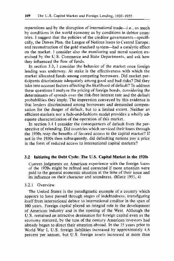
The United States is the paradigmatic example of a country which appears to have passed through stages of indebtedness, transfiguring itself from international debtor to international creditor in the span of 100 years. Foreign capital played an integral role in the development of American industry and in the opening of the West. Although the U.S. remained an attractive destination for foreign capital even as the economy matured, by the turn of the century American investors had already begun to direct their attention abroad. In the 15 years prior to World War I , U.S. foreign liabilities increased by approximately 4.6 percent per annum, but U.S. foreign assets increased at more than
110 Barry Eichengreen
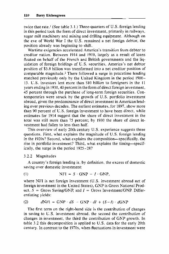
twice that rate.’ (See table 3.1 .) Three-quarters of U.S. foreign lending in this period took the form of direct investment, primarily in railways, sugar mill machinery and mining and drilling equipment. Although on the eve of World War I the U.S. remained a net foreign debtor, the position already was beginning to shift.
Wartime exigencies accelerated America’s transition from debtor to creditor nation. Between 1914 and 1919, largely as a result of loans floated on behalf of the French and British governments and the liq- uidation of foreign holdings of U.S. securities, America’s net debtor position of $3.8 billion was transformed into a net creditor position of comparable magnitude.2 There followed a surge in peacetime lending matched previously only by the United Kingdom in the period 1900- 13. U.S. investors lent more than $10 billion to foreigners in the 11 years ending in 1930,40 percent in the form of direct foreign investment, 45 percent through the purchase of long-term foreign securities. Con- temporaries were struck by the growth of U.S. portfolio investment abroad, given the predominance of direct investment in American lend- ing over previous decades. The earliest estimates, for 1897, show more than 90 percent of U.S. foreign investment to have been direct, while estimates for 1914 suggest that the share of direct investment in the total was still more than 75 percent; by 1930 the share of direct in- vestment had fallen to less than half.
This overview of early 20th century U.S. experience suggests three questions. First, what explains the magnitude of U.S. foreign lending in the 1920s? Second, what explains the composition-specifically, the rise in portfolio investment? Third, what explains the timing-specif- ically, the surge in the period 1925-28?
3.2.2 Magnitudes
saving over domestic investment: A country’s foreign lending is, by definition, the excess of domestic
(1) NFI = S * GNP - I * GNP,
where NFI is net foreign investment (U.S. investment abroad net of foreign investment in the United States), GNP is Gross National Prod- uct, S = Gross Saving/GNP, and I = Gross Investment/GNP. Differ- entiating yields:
(2) dNFI = GNP dS - GNP * d l + ( S - I ) * dGNP
The first term on the right-hand side is the contribution of changes in saving to U.S. investment abroad, the second the contribution of changes in investment, the third the contribution of GNP growth. In table 3.2 this decomposition is applied to U.S. data for the early 20th century. In contrast to the 1970s, when fluctuations in investment were
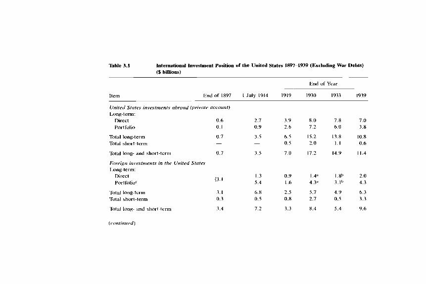
Table 3.1 International Investment Position of the United States 1897-1939 (Excluding War Debts) ($ billions)
End of Year
Item End of 1897 1 July 1914 1919 1930 1933 1939
United States investments abroad (private account) Long-term:
Direct
Portfolio
Total long-term Total short-term
Total long- and short-term
Foreign investments in the United States Long-term:
Direct
PortfolioC
Total long-term Total short-term
Total long- and short-term
0.6 0.1
0.7 -
0.7
(3. I
3. I 0.3
3.4
2.7 0.9
3.5 ~
3.5
1.3 5.4
6.8 0.5
7.2
3.9 2.6
6.5 0.5
7.0
0.9 1.6
2.5 0.8
3.3
8.0 7.2
15.2 2.0
17.2
I .4' 4.3"
5.7 2.7
8.4
7.8 6.0
13.8 1.1
14.9
1 .8b 3.1h
4.9 0.5
5.4
7.0 3.8
10.8 0.6
11.4
2.0 4.3
6.3 3.3
9.6
(continued)
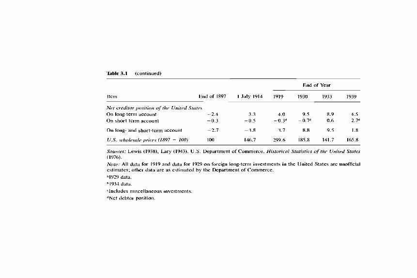
Table 3.1 (continued)
End of Year
Item End of 1897 I July 1914 I919 1930 1933 1939
Net creditor position of the United States On long-term account - 2.4 3.3 4.0 9.5 8.9 4.5
On long- and short-term account - 2.7 - 3.8 3.7 8.8 9.5 1.8
On short-term account -0.3 -0.5 -0.3d -0.7d 0.6 ~ 2 . 7 ~
U S . wholesule priccv (1897 = 100) I00 146.7 299.6 185.8 141.7 165.8
Sourc.es: Lewis (1938), Lary (1943), U.S. Department of Commerce, Mistoricuf Sfutistics of the United Stutes ( 1976).
Nore: All data for 1919 and data for 1929 on foreign long-term investments in the United States are unofficial estimates; other data are as estimated by the Department of Commerce.
"1929 data. h1934 data
'Includes miscellaneous investments. "Net debtor position.
113 The U.S. Capital Market and Foreign Lending, 1920-1955
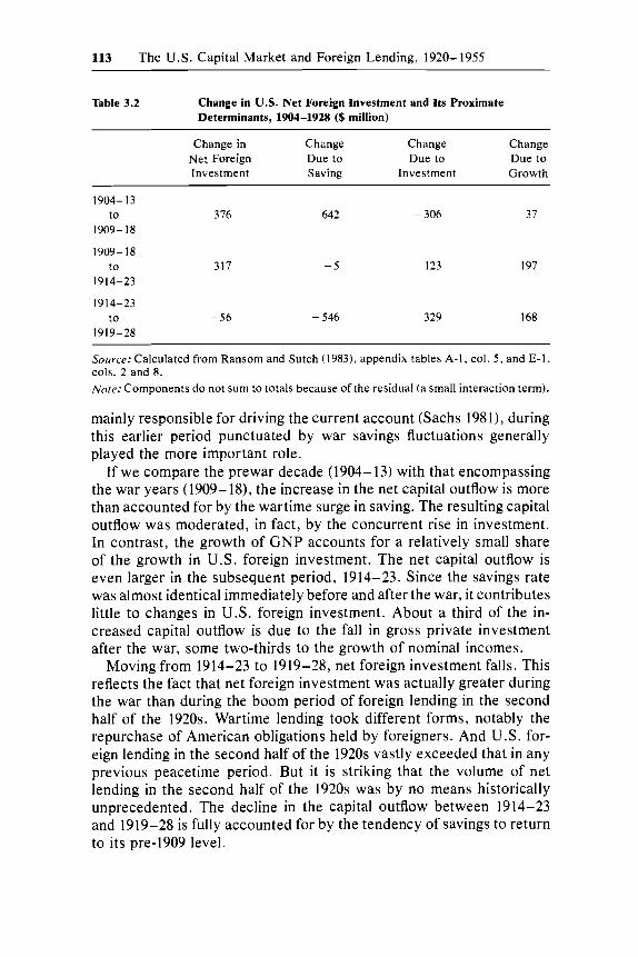
Table 3.2 Change in U.S. Net Foreign Investment and Its Proximate Determinants, 1904-1928 ($ million)
Change in Change Change Change Net Foreign Due to Due to Due to Investment Saving Investment Growth
~
1904-13 to 376 642 - 306 37
1909-18
1909-18 to 3 I7 - 5 123 197
1914-23
1914-23 to - 56 - 546 329 168
19 19-28
Source: Calculated from Ransom and Sutch (1983), appendix tables A-I , col. 5 , and E-I, cols. 2 and 8. Note: Components do not sum to totals because of the residual (a small interaction term).
mainly responsible for driving the current account (Sachs 1981), during this earlier period punctuated by war savings fluctuations generally played the more important role.
If we compare the prewar decade (1904-13) with that encompassing the war years (1909-18), the increase in the net capital outflow is more than accounted for by the wartime surge in saving. The resulting capital outflow was moderated, in fact, by the concurrent rise in investment. In contrast, the growth of GNP accounts for a relatively small share of the growth in U.S. foreign investment. The net capital outflow is even larger in the subsequent period, 1914-23. Since the savings rate was almost identical immediately before and after the war, it contributes little to changes in U.S. foreign investment. About a third of the in- creased capital outflow is due to the fall in gross private investment after the war, some two-thirds to the growth of nominal incomes.
Moving from 1914-23 to 1919-28, net foreign investment falls. This reflects the fact that net foreign investment was actually greater during the war than during the boom period of foreign lending in the second half of the 1920s. Wartime lending took different forms, notably the repurchase of American obligations held by foreigners. And U.S. for- eign lending in the second half of the 1920s vastly exceeded that in any previous peacetime period. But it is striking that the volume of net lending in the second half of the 1920s was by no means historically unprecedented. The decline in the capital outflow between 1914-23 and 1919-28 is fully accounted for by the tendency of savings to return to its pre-1909 level.
114 Barry Eichengreen
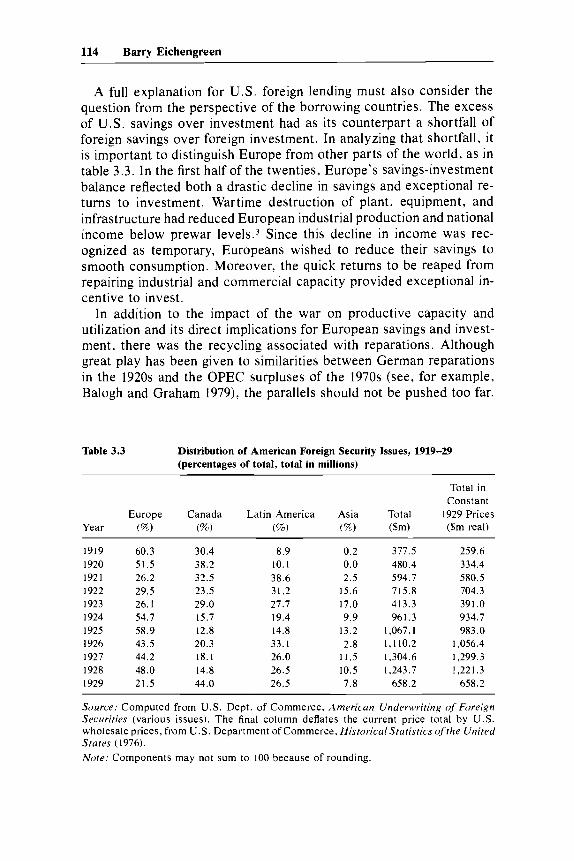
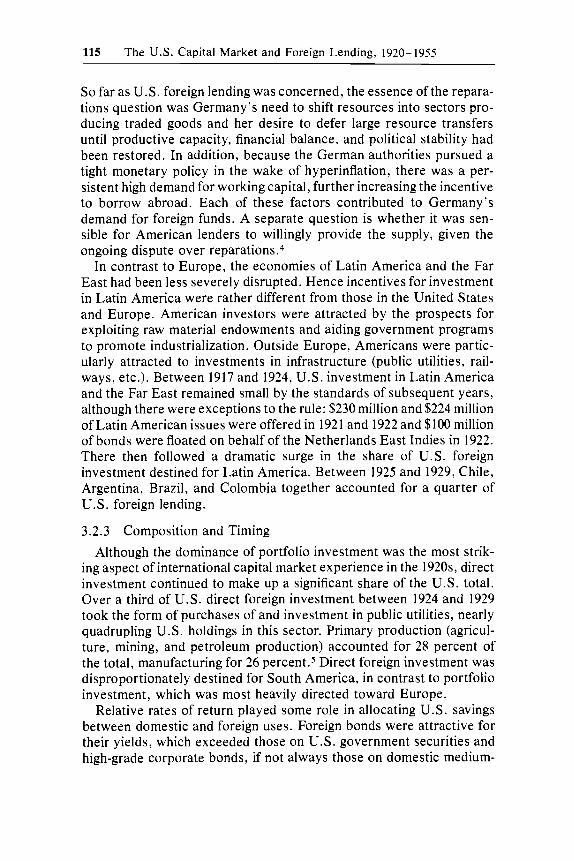
A full explanation for U . S . foreign lending must also consider the question from the perspective of the borrowing countries. The excess of U.S. savings over investment had as its counterpart a shortfall of foreign savings over foreign investment. In analyzing that shortfall, it is important to distinguish Europe from other parts of the world, as in table 3.3. In the first half of the twenties, Europe's savings-investment balance reflected both a drastic decline in savings and exceptional re- turns to investment. Wartime destruction of plant, equipment, and infrastructure had reduced European industrial production and national income below prewar levels.3 Since this decline in income was rec- ognized as temporary, Europeans wished to reduce their savings to smooth consumption. Moreover, the quick returns to be reaped from repairing industrial and commercial capacity provided exceptional in- centive to invest.
In addition to the impact of the war on productive capacity and utilization and its direct implications for European savings and invest- ment, there was the recycling associated with reparations. Although great play has been given to similarities between German reparations in the 1920s and the OPEC surpluses of the 1970s (see, for example, Balogh and Graham 1979), the parallels should not be pushed too far.
Table 3.3 Distribution of American Foreign Security Issues, 1919-29 (percentages of total, total in millions)
Total in Constant
Year (%) (%) (%'c) ($m) ($m real)
1919 60.3 30.4 8.9 0.2 377.5 259.6 1920 51.5 38.2 10.1 0.0 480.4 334.4 1921 26.2 32.5 38.6 2.5 594.7 580.5 1922 29.5 23.5 31.2 15.6 715.8 704.3 1923 26. I 29.0 27.7 17.0 413.3 391 .O 1924 54.7 15.7 19.4 9.9 961.3 934,7 1925 58.9 12.8 14.8 13.2 1,067.1 983 .O 1926 43.5 20.3 33.1 2.8 1,110.2 1,056.4 1927 44.2 18.1 26.0 11.5 1,304.6 1,299.3 1928 48.0 14.8 26.5 10.5 1,243.7 1,221.3 1929 21.5 44.0 26.5 7.8 658.2 658.2
Europe Canada Latin America Asia Total 1929 Prices
Source: Computed from U.S . Dept. of Commerce, American Underwriting of Foreign Securities (various issues). The final column deflates the current price total by U.S. wholesale prices, from U.S. Department of Commerce, Historical Statistics of the United States (1976). Note: Components may not sum to 100 because of rounding.
115 The U.S . Capital Market and Foreign Lending, 1920-1955
So far as U.S. foreign lending was concerned, the essence of the repara- tions question was Germany’s need to shift resources into sectors pro- ducing traded goods and her desire to defer large resource transfers until productive capacity, financial balance, and political stability had been restored. In addition, because the German authorities pursued a tight monetary policy in the wake of hyperinflation, there was a per- sistent high demand for working capital, further increasing the incentive to borrow abroad. Each of these factors contributed to Germany’s demand for foreign funds. A separate question is whether it was sen- sible for American lenders to willingly provide the supply, given the ongoing dispute over reparation^.^
In contrast to Europe, the economies of Latin America and the Far East had been less severely disrupted. Hence incentives for investment in Latin America were rather different from those in the United States and Europe. American investors were attracted by the prospects for exploiting raw material endowments and aiding government programs to promote industrialization. Outside Europe, Americans were partic- ularly attracted to investments in infrastructure (public utilities, rail- ways, etc.). Between 1917 and 1924, U.S. investment in Latin America and the Far East remained small by the standards of subsequent years, although there were exceptions to the rule: $230 million and $224 million of Latin American issues were offered in 1921 and 1922 and $100 million of bonds were floated on behalf of the Netherlands East Indies in 1922. There then followed a dramatic surge in the share of U.S. foreign investment destined for Latin America. Between 1925 and 1929, Chile, Argentina, Brazil, and Colombia together accounted for a quarter of U , S. foreign lending.
3.2 .3 Composition and Timing
Although the dominance of portfolio investment was the most strik- ing aspect of international capital market experience in the 1920s, direct investment continued to make up a significant share of the U.S. total. Over a third of U.S. direct foreign investment between 1924 and 1929 took the form of purchases of and investment in public utilities, nearly quadrupling U.S. holdings in this sector. Primary production (agricul- ture, mining, and petroleum production) accounted for 28 percent of the total, manufacturing for 26 p e r ~ e n t . ~ Direct foreign investment was disproportionately destined for South America, in contrast to portfolio investment, which was most heavily directed toward Europe.
Relative rates of return played some role in allocating U.S. savings between domestic and foreign uses. Foreign bonds were attractive for their yields, which exceeded those on U.S. government securities and high-grade corporate bonds, if not always those on domestic medium-
116 Barry Eichengreen
grade bonds. Despite sterilization by the Federal Reserve, a steady gold influx in conjunction with the expansion of bank credit depressed the returns on domestic assets. After 1921 the rate on bankers’ acceptances declined to less than 4 percent, while call money rates fluctuated be- tween 2 and 5 percent. Domestic bond yields declined from 1923 through 1928. In a period such as 1927-28 when medium-grade domestic bonds yielded only 5.5 percent, foreign bonds which might yield seven or eight percent were understandably attractive.
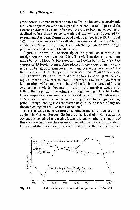
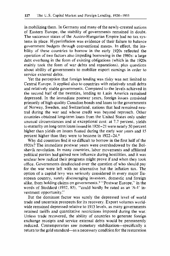
Figure 3.1 shows the relationship of the yields on domestic and foreign dollar bonds over the 1920s. The yield on domestic medium- grade bonds is Moody’s Baa rate, that on foreign bonds Lary’s (1943) sample of 15 foreign issues. Also plotted is the value of new capital issues on behalf of foreign government and corporate borrowers.6 The figure shows that, as the yield on domestic medium-grade bonds de- clined between 1923 and 1927 and that on foreign bonds grew increas- ingly attractive, U.S. foreign lending increased. The fall in U.S. foreign lending after 1927 coincides similarly with a fall in the spread of foreign over domestic yields. Yet rates of return by themselves account for little of the variation in the volume of foreign lending. The role of other factors-specifically risk-is especially evident before 1924, when many U.S. investors seem to have been unwilling to lend to foreigners at any price. Foreign lending rises thereafter despite the absence of any no- ticeable change in relative rates of return.’
The risks which deterred foreign lending in the early 1920s are most evident in Central Europe. So long as the level of their reparations obligations remained uncertain, it was unclear whether the nations of this region would have the resources needed to service additional debt. If they had the resources, it was not evident that they would succeed
Yield on 30 Domestic Medium-Grade Bonds - - 1 6
14
12
I922 1923 1924 1925 I926 1927 1928 1929
Fig. 3.1 Relative interest rates and foreign issues, 1922- 1929
117 The U.S. Capital Market and Foreign Lending, 1920-1955
in mobilizing them. In Germany and many of the newly-created nations of Eastern Europe, the stability of governments remained in doubt, The successor states of the Austro-Hungarian Empire had no tax sys- tems in place. Hyperinflation was evidence of their failure to balance government budgets through conventional means. In effect, the ina- bility of these countries to borrow in the early 1920s reflected the operation of two factors also impeding borrowing in the 1980s: a large debt overhang in the form of existing obligations (which in the 1920s mainly took the form of war debts and reparations), plus questions about ability of governments to mobilize export earnings in order to service external debts.
Yet the perception that foreign lending was risky was not limited to Central Europe. It applied also to countries with relatively small debts and relatively stable governments. Compared to the levels achieved in the second half of the twenties, lending to Latin America remained depressed. In the immediate postwar years, foreign issues consisted primarily of high-quality Canadian bonds and loans to the governments of Norway, Sweden, and Switzerland, nations that had remained neu- tral during the war and whose credit was beyond reproach. Other countries obtained long-term loans from the United States only under unusual circumstances and at exceptional cost: at 7.7 percent, yields to maturity on long-term loans issued in 1920-21 were nearly 50 percent higher than yields on issues floated during the early war years and 15 percent higher than they were to become in 1922-24.*
Why did countries find it so difficult to borrow in the first half of the 1920s? The immediate postwar years were overshadowed by the Bol- shevik revolution. In many countries, labor movements and affiliated political parties had gained new influence during hostilities, and it was unclear how radical their programs might prove if and when they took office. Governments deadlocked over the question of who should pay for the war were left with no alternative but the inflation tax. The option of a capital levy was seriously considered in every major Eu- ropean country, surely discouraging investors, domestic and foreign alike, from holding claims on government^.^ “Postwar Europe,” in the words of Stoddard (1932, 85), “could hardly be rated as an ‘A-1’ in- vestment opportunity.”
But the dominant factor was surely the depressed level of world trade and uncertain prospects for its recovery. Export volumes world- wide remained depressed relative to 1913 levels, as many governments retained tariffs and quantitative restrictions imposed during the war. Unless trade recovered, the ability of countries to generate foreign exchange receipts and service external debts would be permanently reduced. Contemporaries saw monetary stabilization-specifically a return to the gold standard-as a necessary condition for the restoration
118 Barry Eichengreen
of domestic prosperity and the reduction of restrictions needed for the recovery of trade. Only with the termination of Central European hy- perinflations, capped by Germany’s stabilization in 1923-24, and the international movement back onto the gold standard did investors con- clude that trade ultimately would recover and did the capital markets take heart.
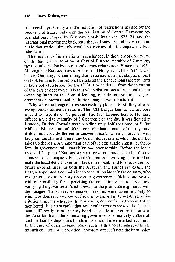
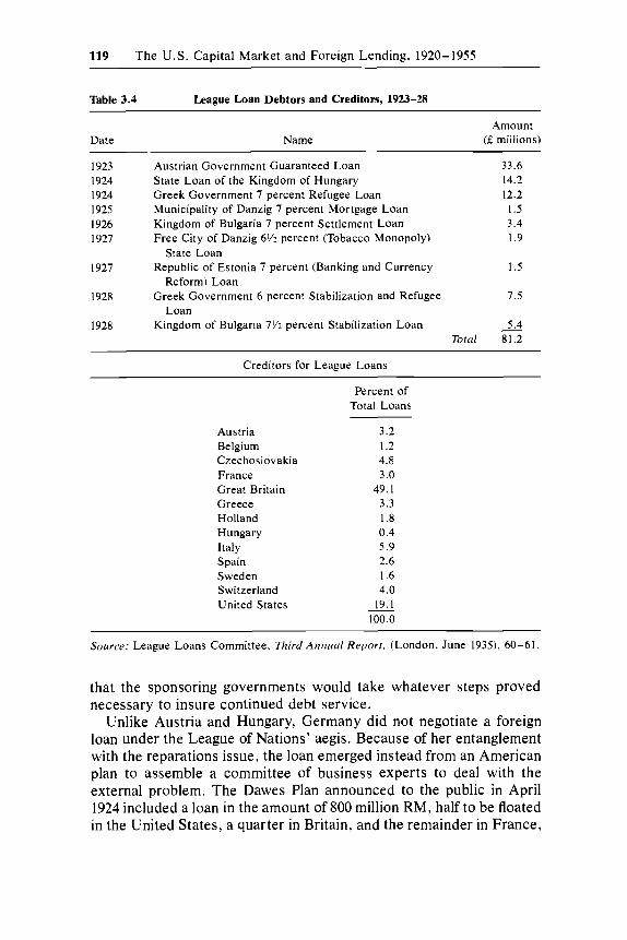
The recovery of international trade hinged, in the view of observers, on the financial restoration of Central Europe, notably of Germany, the region’s leading industrial and commercial power. Hence the 1923- 24 League of Nations loans to Austria and Hungary and the 1924 Dawes loan to Germany, by cementing that restoration, had a catalytic impact on U.S. lending to the region. (Details on the League loans are provided in table 3.4.) If a lesson for the 1980s is to be drawn from the initiation of this earlier debt cycle, it is that when disruptions to trade and a debt overhang interrupt the flow of lending, outside intervention by gov- ernments or international institutions may serve to restart it.
Why were the League loans successfully placed? First, they offered exceptionally attractive returns. The 1923 League loan to Austria bore a yield to maturity of 7.8 percent. The 1924 League loan to Hungary offered a yield to maturity of 8.6 percent; on the day it was floated in London, British Consols were yielding only half that amount.’O But while a risk premium of 100 percent eliminates much of the mystery, it does not provide the entire answer. Insofar as risk increases with the premium charged, there may be no interest rate at which the market takes up the loan. An important part of the explanation must lie, there- fore, in governmental supervision and sponsorship. Before the loans received League of Nations support, governments engaged in discus- sions with the League’s Financial Committee, involving plans to elim- inate the fiscal deficit, to reform the central bank, and to strictly control future expenditures. In both the Austrian and Hungarian cases, the League appointed a commissioner-general, resident in the country, who was granted extraordinary access to government officials and vested with responsibility for supervising the collection of loan service and verifying the government’s adherence to the protocols negotiated with the League. Thus, very extensive measures were taken not only to eliminate domestic sources of fiscal imbalance but to establish an in- stitutional means whereby the borrowing country’s progress might be monitored. It is no surprise that potential investors viewed the League loans differently from ordinary bond issues. Moreover, in the case of the Austrian loan, the sponsoring governments effectively collateral- ized the loan by depositing bonds in its amount in earmarked accounts. In the case of other League loans, such as that to Hungary, although no such collateral was provided, investors were left with the impression
119 The U.S. Capital Market and Foreign Lending, 1920-1955
Table 3.4 League Loan Debtors and Creditors, 1923-28
Date Name Amount
(f millions)
1923 1924 1924 1925 I926 I927
1927
I928
1928
Austrian Government Guaranteed Loan State Loan of the Kingdom of Hungary Greek Government 7 percent Refugee Loan Municipality of Danzig 7 percent Mortgage Loan Kingdom of Bulgaria 7 percent Settlement Loan Free City of Danzig 6Y2 percent (Tobacco Monopoly)
Republic of Estonia 7 percent (Banking and Currency
Greek Government 6 percent Stabilization and Refugee
Kingdom of Bulgaria 7% percent Stabilization Loan
State Loan
Reform) Loan
Loan
33.6 14.2 12.2
1.5 3.4 1.9
1.5
7.5
5.4 Totd 81.2
-
Creditors for League Loans
Percent of Total Loans
Austria Belgium Czechoslovakia France Great Britain Greece Holland Hungary Italy Spain Sweden Switzerland United States
3.2 1.2 4.8 3.0
49.1 3.3 1.8 0.4 5.9 2.6 1.6 4.0
19.1 100.0
Source: League Loans Committee, Third Annucil Report, (London, June 1935). 60-61.
that the sponsoring governments would take whatever steps proved necessary to insure continued debt service.
Unlike Austria and Hungary, Germany did not negotiate a foreign loan under the League of Nations’ aegis. Because of her entanglement with the reparations issue, the loan emerged instead from an American plan to assemble a committee of business experts to deal with the external problem. The Dawes Plan announced to the public in April 1924 included a loan in the amount of 800 million RM, half to be floated in the United States, a quarter in Britain, and the remainder in France,
120 Barry Eichengreen
Belgium, Holland, Italy, Sweden, and Switzerland. As with the League loans, the market’s response was overwhelming. The issue was over- subscribed in Britain by a factor of 13, in New York by a factor of 10.
The enthusiasm with which American investors took up the Dawes loan is striking in the light of earlier skepticism about European floa- tations. Even the bankers had greeted the plan with considerable skep- ticism. In part, success resulted from propitious financial market conditions. The Federal Reserve discount rate had been reduced in the spring of 1924 by an exceptionally large amount, from 4.5 to 3 percent, rendering foreign investments attractive for their return. I ’ The Amer- ican tranche was sold to the public at 92, to be redeemed at 105; together with a nominal interest rate of 7 percent, this meant that it yielded 7.6 percent. In addition, the U.S. government and New York banks had pressed for British and French involvement, partly to create domestic interests in those countries that would oppose giving priority to repara- tions over commercial liabilities. Involving foreign investors increased U.S. confidence that Dawes loan obligations would not be subordinated to reparations. A final explanation for the success of the loan lies in the aggressive publicity campaign launched in its support. Even Pres- ident Coolidge urged patriotic American investors to subscribe.
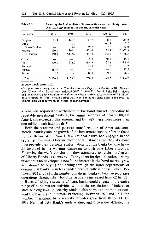
These measures were used to buttress financial stability in Europe and to ensure the restoration of international trade, and once launched they continued to operate on their own. For many investors, foreign dollar bonds had been until recently an unfamiliar instrument. But American investors grew accustomed to holding bonds through the good offices of the U.S. Treasury, which aggressively administered the Liberty Loan campaign during World War I. Under the Liberty Loan Act of 1917, the Secretary of the Treasury was authorized to purchase obligations of foreign governments at war with enemies of the United States. U.S. purchases of foreign securities were financed by selling the American public dollar-denominated securities in matching amounts. The rate of interest charged the European borrowers was simply the rate required by American investors plus a small spread to cover costs. American investors encouraged to subscribe by extensive publicity campaigns did so in the amounts shown in table 3.5. “Millions of individuals who had never clipped a coupon or owned a share of stock, now became “investment-minded’’ for the first time in their lives.”12
American investors’ appetite for foreign bonds having been awak- ened, changes in the scope and structure of U.S. financial markets helped to satisfy it. Sales of foreign dollar bonds were buoyed by the growth of the investing public. In 1914, by one estimate, there were no more than 200,000 American bond buyers in a market limited largely to Boston and its e n ~ i r 0 n s . l ~ But by 1922, when an income of $5,000
121 T h e U.S. Capital Marke t and Foreign Lending, 1920-1955
Table 3.5 Loans by the United States Government, under the Liberty Loan Act, 1917-22’ (millions of dollars, calendar years)
Borrower 1917 1918 1919 1920-22 Total
Belgium Cuba Czechoslovakia France Great Britain
Greece Italy Rumania Russia Serbia
Total
75.4 - -
1,130.0 1,860.7
- 400.0
187.7 3.0
3,656.8
-
141.6 10.0 5.0
966.4 2.122.0
- 776.0 - -
7.8
4,028.8
121.7
49.3 801.0 287.4
5.0 444.9
25.0
16.0
1,750.3
8.5 -2.3
7.7 35.9
- 133.6
10.0 27.1 - 1.8
-0.7
-49.2
347.2 7.7
62.0 2,933.3 4,136.5
15.0 1,648.0
23.2 187.7 26.1
9,386.7
Source: Lewis (1938, 362). Compiled from data given in the Combined Annual Reports of the World War Foreign Debt Commission, Fiscal Years 1922-26 (1927, 2, 318-25). For 1919 the British figure and the total are both net, after deductions have been made to take account of 7.6 million dollars repaid by Great Britain during that year. The minus signs used in the 1920-22 column indicate repayments in excess of cash advances.
a year was required to participate in the bond market, according to reputable investment bankers, the annual incomes of nearly 600,000 Americans exceeded this amount, and by 1929 there were more than one million such individuals. I 4
Both the wartime and postwar transformation of American com- mercial banking and the growth of the investment trust reinforced these trends. Before World War I , few national banks had engaged in the securities business. Only in exceptional instances did they do more than provide their customers information. But the banks became heav- ily involved in the wartime campaign to distribute Liberty Bonds. Following the war’s conclusion, they attempted to retain purchasers of Liberty Bonds as clients by offering them foreign obligations. Many investors who developed a newfound interest in the bond market grew accustomed to buying and selling through the bond departments of commercial banks, which expanded dramatically in consequence. Be- tween 1922 and 193 1, the number of national banks engaged in securities operations through their bond departments increased from 62 to 123.
By establishing a security affiliate, banks could engage in the entire range of bond-market activities without the restrictions of federal or state banking laws. A security affiliate also permitted them to circum- vent the barriers to interstate branching. Between 1922 and 1931, the number of national bank security affiliates grew from 10 to 114. By 1919 National City Bank’s underwriting and brokerage affiliate, the
122 Barry Eichengreen
City Company, had opened branch offices in 51 cities, often on the ground floor to encourage walk-in business. It publicized the attractions of a bond portfolio through advertisements in popular magazines such as Harper’s and Atlantic Monthly.
Banks and their affiliates took an active role not only in retailing but in the origination of foreign bond issues. In the 1920s American banks for the first time expanded overseas on a significant scale. Prior to the passage of the Federal Reserve Act, national banks had been prohibited from branching abroad. Although private banks and some state banks were permitted to do so, as late as 1914 there existed only 26 foreign branches of American banks. The Federal Reserve Act relaxed the constraint on foreign branching, however, and World War I, by dis- rupting the ability of European banks to extend export credits, provided the impetus for American banks to move overseas. Although some retrenchment occurred in the years to follow, by 1920 the number of foreign branches of U.S. banks had increased to 181. These branches provided a steady stream of contacts between American bankers and potential foreign borrowers.I5
The need for a diversified portfolio, impressed upon potential pur- chasers by responsible salesmen, limited the involvement of the small investor. I 6 Increasingly, however, this constraint was relaxed by the growth of the investment trust. A forerunner of the modern mutual fund, the investment trust pooled the subscriptions of its clients, placed their management in the hands of specialists, and issued long-term securities entitling holders to a share of the organization’s earnings. The modern investment trust originated largely in Britain, where it traditionally specialized in foreign bonds. When the investment trust first appeared on a significant scale in the United States after 1921, many of the new institutions followed British example by investing heavily in foreign bonds.I8
Thus, in the 1920s as in the 1970s, the surge in foreign lending was greatly facilitated by financial innovation. The rapid development of retailing and underwriting activities and the proliferation of investment vehicles provided financial organizations both incentive and opportu- nity to increase their participation in foreign bond markets. While the growth of the investing public and the low yields on domestic bonds created an incipient demand for foreign assets, competition among financial institutions provided the supply. It has been asserted, follow- ing Hiram Johnson, head of the Senate’s 1931-32 Foreign Bond In- vestigation, that these institutions competed excessively, pushing loans on inexperienced foreign governments and forcing bonds on naive do- mestic investors. l 9 The banking community counters that established firms with reputations to protect had no incentive to promote ques- tionable investments, since “such securities would damage the under-
123 The U . S . Capital Market and Foreign Lending, 1920-1955
writer’s credibility with investors, making it more difficulty for the underwriter to sell securities in the future.”20 While this logic is im- peccable, it may apply imperfectly to the 1920s by virtue of the fact that many institutional participants in international bond markets were recent entrants with little if any reputation to protect. The model fits better in Britain, where the underwriting of foreign securities was han- dled almost exclusively by a small number of long-established firms that agreed to limit the extent of competition, dividing the field “among themselves and develop[ing] more or less permanent financing arrange- ments with various foreign issuers.”*I In the United States, a distinctive feature of the market environment in the 1920s was the extent of entry. Mintz (1951) notes that the loans issued by various groups of banking houses in the 1920s fared very differently, with only 14 percent of the (non-Canadian) loans issued by three participants ultimately defaulting, but nearly 90 per cent of the loans issued by six other banking houses falling into default. Although Mintz is careful not to identify the banking houses, the timing of their loans suggests that the first group was com- posed of long-time participants and the second of recent entrants. One might speculate that firms in the second group were simply less well managed, but it is also likely that their managements were more inclined toward risky issues since they had less reputation to lose in the event of default. If, in the long run, track record in comparison with incum- bants will drive unsuccessful entrants out of the market, there is no reason to suppose that these forces had much effect between 1921 and 1929.
Critics blamed loan pushing on lax regulation by public authorities. Until 1933 many of the operations of securities affiliates remained un- regulated. The popular argument, especially after the Wall Street crash and the onset of default, was that the establishment of bank security affiliates brought into conflict the bank’s obligation to provide prudent advice to its depositor-investors and its desire to sell the security issues it originated. Even if the affiliate did not unduly favor the securities of its customers, with a bond distribution network in place the affiliates had an interest in promoting the sale of bonds even when the supply of high-quality issues declined. This notion that the establishment of affiliates led the banks to encourage reckless investment in foreign bonds contributed to the passage in 1933 of the Glass-Steagall Act outlawing the security affiliate.22
The U.S. State and Commerce Departments also can be criticized for inadequately screening individual loans. Banks originating foreign loans were asked only to consult the State Department prior to offering an issue to American investors. The State Department then consulted with the Treasury and Commerce Departments before announcing whether or not it had an objection. While the program was voluntary,
124 Barry Eichengreen
bankers hesitant to cooperate risked incurring the wrath of the admin- istration and losing its assistance in the event of default. Critics such as Senator Carter Glass of Virginia complained that the program was at the same time insufficiently stringent to prevent dubious foreign loans and insufficiently clear to prevent potential investors from in- terpreting a statement of “no objection” as the government’s seal of
The government’s activities involved both education and data gath- ering. Its agents furnished information on particular enterprises and investment projects, which the department mailed to hundreds of American banks. These agents were sometimes able in their official capacity to obtain financial information to which the bankers did not have access. Hence many U.S. banks came to rely on assessments by Commerce Department agents of potential foreign investment projects as part of normal business practice.24
The principal instances in which the U.S. authorities made use of their oversight of foreign lending were in connection with foreign gov- ernments owing war debts to the United States.25 A strict loan embargo was imposed against the Soviet Union. Washington disapproved a pro- spective Romanian loan in 1922 because of the absence of a war debt funding agreement. It disapproved of refunding issues for France until that country negotiated a war debt settlement. Naturally, this policy proved unpopular in Europe, the French threatening for example to impose a tariff on U.S. automobiles, which led in 1928 to permission to float French industrial securities on the American market.26 This was only a particular instance of a general phenomenon, that “[iln almost all cases where the government entered an objection, it could be gotten round or in time removed” (Feis 1950, 13).
Compared to their attitude toward other countries, U.S. authorities were surprisingly lenient in their treatment of German loans. While Commerce Department agents in Berlin continually reminded Wash- ington of the magnitude of the reparations burden and of the danger that Germany would be unable to both pay reparations and service municipal and corporate loans, the position of the U.S. authorities remained ambiguous. Commerce continued to supply the leading in- vestment houses with information on the finances of municipalities and even the prospects for specific investment projects. While the warnings of its agents were passed on to the U.S. investment banking community, few if any German loan applications met with formal objection. Starting in 1925, the Commerce and State Departments issued somewhat am- biguous warnings to the bankers. The State Department alluded to the possibility of an embargo on loans to German states and municipalities in instances where such loans might hamper transfers under the Dawes Plan. 27
125 The U.S. Capital Market and Foreign Lending, 1920-1955
While the Department of State raises no objection to this flotation . . . it feels that American bankers should know that the amount of German loans has become so large, and the control of exchange on behalf of the Allies is such, as to raise a question as to whether or not it may be very difficult for German borrowers to make the nec- essary transfers.**
Why was German borrowing treated so leniently? It is not that Commerce Department officials failed to recognize the danger of de- fault. As early as 1925 internal memoranda warned of an investment “debacle,” and in 1928 the problem had achieved such proportions that middle-ranking officials were warned to distance themselves from German lending to protect the government in the event of default.29 But the State Department overrode the hesitations of Commerce out of a desire to maintain German stability as a bulwark against Bolshe- vism. Moreover, Andrew Mellon, secretary of the treasury for much of the 1920s, actively represented the bankers’ desire that German lending be left unfettered. And ultimately, U.S. officials believed deeply in the laissez-faire approach to foreign lending-that the market knew best.
3.3 Pricing Foreign Debt
Why did these people lend money to Austria, or Japan, or Germany, or Argentine, or Belgium? Here, statistics are of little value. Men have not yet found a way of measuring the motives of other men. (Morrow 1927)
A standard criticism of the international capital market in the 1920s is that it failed to discriminate adequately among borrowers. Precisely the same criticism has been leveled at U.S. creditors in the 1970s; Guttentag and Herring (1985) argue that rates charged sovereign bor- rowers on bank loans could not have adequately incorporated the de- terminants of country-risk premia because they varied so little across loans. Edwards (1986) has attempted to test this hypothesis formally for both bank loans and bonds, using regression to analyze the rela- tionship between ex ante spreads and correlates of the country-risk premium such as debt, reserves, investment, the current account, and imports as shares of GNP, the ratio of debt service to exports, the rate of economic growth, the real exchange rate, and characteristics of the borrower and the loan. His results for the bond market were mixed: rates charged borrowers were found to rise with the debt/GNP ratio, to fall with the investment/GNP ratio, and to decline with the maturity of the loan. The first two of these results are consistent with the notion
126 Barry Eichengreen
that bondholders distinguished among good and bad credit risks. The coefficients on the other variables were uniformly insignificant, how- ever, suggesting that investors paid little attention to other plausible indicators of country risk when pricing foreign bonds.
These results provide a benchmark for comparison with my analysis of the bond market in the 1920s. To analyze the determinants of the ex ante rate of return required by bondholders in the 192Os, I employ data on the yield to maturity on issue for bonds floated in the United States between 1920 and 1929. These data, compiled by Lewis (1938), include all foreign securities issued and taken in the United States, both securities publicly issued and privately taken. They exclude por- tions of such issues sold on foreign markets (so far as could be deter- mined) and securities of American-controlled enterprises (which are considered direct investment), thereby differing from other sources of information on the subject such as the Department of Commerce’s lists of foreign loans. (Both public and private issues are similarly included in modern studies such as Edwards’s.) The par value of loans and the yield to maturity are provided by year of issue, domicile of borrower, maturity (long-term loans versus short-term loans of five years or less), and type of borrower (national and provincial, municipal or corporate). For the 1920s the required information is provided for 383 categories of bonds. These data were then linked to information on the charac- teristics of the borrowing countries. It was not possible to obtain in- formation on all of the independent variables used in modern analyses, regrettably insofar as this renders the results to follow imperfectly comparable. But just as estimates of national income, investment and related variables for the 1920s are not available to historians, such estimates were not available to bondholders and hence were unlikely to be used in pricing foreign bonds. The readily-available indicators of policy stance were foreign trade and public finance statistic^.^^ I there- fore use the trade and budget balances as measures of domestic policy. Contemporaries argued that a balance-of-trade surplus should have been related negatively to the required rate of return on bonds, as the larger the surplus the greater the export receipts available for debt service. Similarly, a government budget surplus should have been neg- atively associated with the required rate, as any budget surplus could be used to retire domestic debt and reduce the government’s total debt burden.31 Data on these variables were drawn from publications of the League of Nations for 221 of Lewis’s 383 observation^.^^ Trade and budget surpluses are measured as shares of imports and government expenditures, respectively.
The dependent variable is the spread over domestic risk-free rates, defined as the foreign yield minus the yield on securities rated Baa by Moody’s (annual averages). The value of the loan is divided by the
127 The U.S. Capital Market and Foreign Lending, 1920-1955
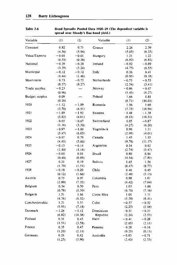
value of exports to control for country size.33 Regression results are reported in table 3.6. The omitted alternatives (1929, Venezuela, and corporation) are picked up by the constant term.34 The spread varies considerably, with a mean of 0.46 and a standard deviation of 1.20. According to the regressions, the yield on short-term loans averaged 73 basis points below that on long term loans. Although this result contrasts with that obtained by Edwards for the 1970s, who found the yield on short-term bonds to be higher than that on long-term issues, it is consistent with the presumption that the yield curve should be positively sloped. The negative coefficients on public loans (both sov- ereign and municipal) indicates that the public demanded a smaller risk premium for them than on corporate bonds. This contrasts with Ed- wards’s (1986) finding for the 1970s of no discernible difference.
The remaining variables are dummies for countries, trade and budget balances, and dummies for years prior to 1929. The first can be inter- preted as proxies for national reputation, the second as proxies for current policy, the third as components of the spread not attributable to other characteristics of the loans. The coefficients on years indicate some tendency for the spread to rise over the course of the 1920s, as if market participants recognized the increasingly risky nature of for- eign loans. According to the country dummies, the best bond-market reputations were enjoyed, not surprisingly, by Scandinavian countries (Denmark, Norway, Sweden), members of the British Commonwealth (Australia, Canada, Ireland), small Western European countries (Swit- zerland, the Netherlands), and small Central American republics eco- nomically or politically dependent on the United States (Cuba, the Dominican Republic, Haiti, Panama).35 There were good reasons to expect these countries to service their obligations promptly; bond- holders’ willingness to lend to them at favorable rates indicates some significant ability to discriminate among potential borrowers. Con- versely, high rates were charged the new nations of Eastern Europe (Bulgaria, Czechoslovakia, Hungary, Poland, Rumania), a country en- gaged in an international dispute (Greece), and Latin American nations with a history of debt service disruptions (Bolivia, Peru). Again, given the political and economic situation in these countries and, in the case of Latin America, their past record of servicing debt, bondholders’ tendency to demand a risk premium indicates some ability to discrim- inate among borrowers. At the same time, the relatively small risk premia charged Germany, the leading borrower of American funds, and a number of the larger South American republics raise questions about whether bondholders discriminated adequately.
The coefficients on the trade and budget balances provide additional information relevant to this question. While the coefficient on the trade surplus is negative as anticipated, it differs insignificantly from zero.
128 Barry Eichengreen
Table 3.6 Bond Spreads: Pooled Data 1920-29 (The dependent variable is spread over Moody’s Baa bond yield.)
Constant
ValueiExports
National
Municipal
Short-term
Trade surplus
Budget surplus
I920
1921
1922
I923
1924
I925
I926
I927
1928
Austria
Belgium
Bulgaria
Czechoslovakia
Denmark
Finland
France
Germany
0.82 (4.56)
-0.01 (0.53)
-0.29 (3.29)
-0.12 ( I .44) - 0.73
(8.37)
(0.96) 0.09
(0.26) -1.12 (3.70) - 1.89 (3.82)
(3.16) - 0.97
(5.47) -0.67 (4.65)
-0.13 (1.10) - 0.05
(0.40) 0.21
( I .70) -0.18 (0.12) 0.75
(2.80) 0.34
(0.78) 1.51
(4.76) 1.21
(5.95) - 1.26 (6.82) 0.31
(1.51) 0.35
(1.20) 0.26
(1.25)
-0.23
-0.65
0.71 (5.94)
-0.01 (0.38)
-0.28 (3.24)
-0.12 ( I .46)
-0.73 (8.27) -
-
- 1.09 (4.51)
(4.01) - 0.67 (3.30) - 1.00 (6.05) - 0.70
(5.00)
- 1.92
-0.14 (1.16) 0.01
(0.09) 0.19
(1.51) -0.20
( I .66) 0.97
(7.32) 0.50
( I .30) 1.66
(6.32) 1.31
(7.18) -1.12 (10.38)
0.45 (3.58) 0.47
(2.11) 0.42
(3.90)
Greece
Hungary
Ireland
Italy
Netherlands
Norway
Poland
Rumania
Sweden
Switzerland
Yugoslavia
Canada
Argentina
Brazil
Bolivia
Chile
Colombia
Peru
Costa Rica
Cuba
Dominican Republic
Haiti
Panama
Australia
2.26 (5.05) 1.21
(6.82) -0.82 (4.75) 0.26
(0.95)
(2.54) -0.86 (3.45) 1.66
(8.71) 1.56
(7.75) - 1.48 (8.13) - 1.05
(4.27) 0.96
(2.99)
(9.78) 0.54
(2.74) 0.80
(4.54) I .65
(8.47) 0.46
(2.48) 0.88
(4.42) 1.03
(6.70) I .01
(5.38) - 0.57 (2.25)
(2.24)
(2.05)
(0.23)
(2.43)
- 0.73
- 1.45
-0.31
-0.41
- 0.28
- 0.83
2.39 (6.35)
I .22 (6.82)
-0.89 (6.55) 0.41
(0.18) -0.53 (3.41) - 0.67 (6.27) I .81
(16.03) I .69
(10.94)
(10.51) - 0.87 (6.20)
1 . 1 1 (4.01) - 1.35 (11.17)
0.62 (3.47) 0.94
(7.81) I .56
(8.77) 0.45
(3.13) I .01
(7.64) I .00
(7.16) 1 . 1 1
(8.41) -0.52
(2.18) - 0.2 I (2.55)
-0.28 (2.1 I )
-0.16 (0.13)
(2.75)
- 1.38
-0.71
129 The U.S. Capital Market and Foreign Lending, 1920-1955
Table 3.6 (continued)
Japan 0.21 0.36 Number of 221 22 I (0.91) (2.71) observations
RZ .88 .88
Source: See text. Notes: White-corrected ?-statistics in parentheses. The omitted alternatives are 1929, Venezuela, and corporations.
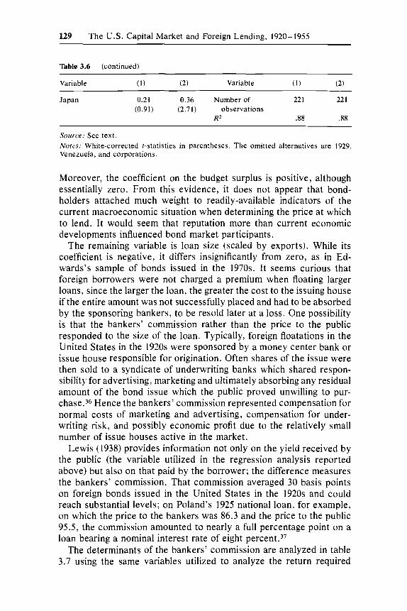
Moreover, the coefficient on the budget surplus is positive, although essentially zero. From this evidence, it does not appear that bond- holders attached much weight to readily-available indicators of the current macroeconomic situation when determining the price at which to lend. It would seem that reputation more than current economic developments influenced bond market participants.
The remaining variable is loan size (scaled by exports). While its coefficient is negative, it differs insignificantly from zero, as in Ed- wards’s sample of bonds issued in the 1970s. It seems curious that foreign borrowers were not charged a premium when floating larger loans, since the larger the loan, the greater the cost to the issuing house if the entire amount was not successfully placed and had to be absorbed by the sponsoring bankers, to be resold later at a loss. One possibility is that the bankers’ commission rather than the price to the public responded to the size of the loan. Typically, foreign floatations in the United States in the 1920s were sponsored by a money center bank or issue house responsible for origination. Often shares of the issue were then sold to a syndicate of underwriting banks which shared respon- sibility for advertising, marketing and ultimately absorbing any residual amount of the bond issue which the public proved unwilling to pur- chase.36 Hence the bankers’ commission represented compensation for normal costs of marketing and advertising, compensation for under- writing risk, and possibly economic profit due to the relatively small number of issue houses active in the market.
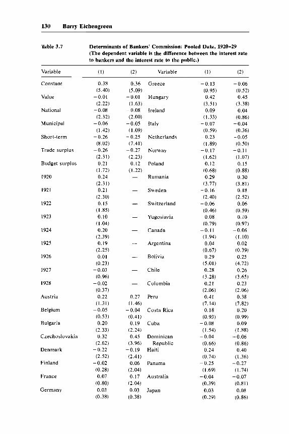
Lewis (1938) provides information not only on the yield received by the public (the variable utilized in the regression analysis reported above) but also on that paid by the borrower; the difference measures the bankers’ commission. That commission averaged 30 basis points on foreign bonds issued in the United States in the 1920s and could reach substantial levels; on Poland’s 1925 national loan, for example, on which the price to the bankers was 86.3 and the price to the public 95.5, the commission amounted to nearly a full percentage point on a loan bearing a nominal interest rate of eight percent.37
The determinants of the bankers’ commission are analyzed in table 3.7 using the same variables utilized to analyze the return required
130 Barry Eichengreen
Table 3.7 Determinants of Bankers’ Commission: Pooled Data, 1920-29 (The dependent variable is the difference between the interest rate to bankers and the interest rate to the public.)
Variable ( 1 ) (2) Variable (1) (2)
Constant
Value
National
Municipal
Short-term
Trade surplus
Budget surplus
I920
1921
1922
1923
1924
1925
1926
I927
1928
Austria
Belgium
Bulgaria
Czechoslovakia
Denmark
Finland
France
Germany
0.38 (5.40)
-0.01 (2.22) - 0.08 (2.32) - 0.06
( I .42)
(8.02) -0.26
(2.31) 0.21
(1.72) 0.24
(2.31) 0.21
(2.30) 0.15
(1.85) 0.10
(1.04) 0.20
(2.39) 0.19
(2.25) 0.01
(0.23) - 0.03 (0.96) - 0.02 (0.37) 0.22
(1.31) - 0.05 (0.53) 0.20
(2.33) 0.32
(2.62) - 0.22
(2.52) -0.02 (0.28) 0.07
(0.80) 0.03
(0.38)
-0.26
0.36 Greece (5.09)
-0.01 Hungary ( I .63)
-0.08 Ireland (2.00)
-0.05 Italy (I .09)
-0.25 Netherlands (7.41)
-0.27 Norway (2.23) 0.12 Poland (I .22) - Rumania
- Sweden
- Switzerland
- Yugoslavia
- Canada
- Argentina
- Bolivia
- Chile
- Colombia
0.27 Peru ( I .46)
(0.41) 0.19 Cuba
(2.24) 0.45 Dominican
(3.96) Republic
(2.41) 0.06 Panama
(2.04) 0.17 Australia
(2.04) 0.03 Japan
(0.38)
-0.04 Costa Rica
-0.19 Haiti
-0.13 (0.95) 0.42
(3.51) 0.09
(1.33) - 0.07
(0.59)
( I .89) -0.17
( I .62) 0.12
(0.68) 0.29
(3.77)
(2.40) -0.06
(0.46) 0.08
(0.79) -0.11
( I .94) 0.04
(0.67) 0.29
(5.01) 0.28
(3.28) 0.21
(2.06) 0.41
(7.14) 0.18
(0.93) - 0.08 (1.54) - 0.04 (0.66) 0.24
(0.74)
(I .69)
(0.39) 0.03
(0.29)
- 0.23
-0.16
-0.25
- 0.04
-0.06 (0.52) 0.45
(3.38) 0.04
(0.86)
(0.36) -0.05 (0.50)
-0.11 ( I .07) 0. I5
(0.88) 0.30
(3.81) -0.18 (2.52) 0.06
(0.59) 0.10
(0.97) -0.06 (1.10) 0.02
(0.39) 0.25
(4.72) 0.26
(3.65) 0.23
(2.06) 0.38
(7.82) 0.20
(0.99) -0.09
( I ,881 - 0.06
(0.86) 0.40
(1.36) -0.27 (1.74) - 0.07 (0.81) 0.08
(0.86)
- 0.04
131 The U.S. Capital Market and Foreign Lending, 1920-1955
Table 3.7 (continued)
Brazil 0.05 0.04 Number of 22 1 22 1
R* .58 .52 (0.59) (0.48) observations
Source: See text. Notes: Ordinary least squares regressions with White-corrected ?-statistics in parenthe- ses, The omitted alternatives are 1929, Venezuela, and corporations.
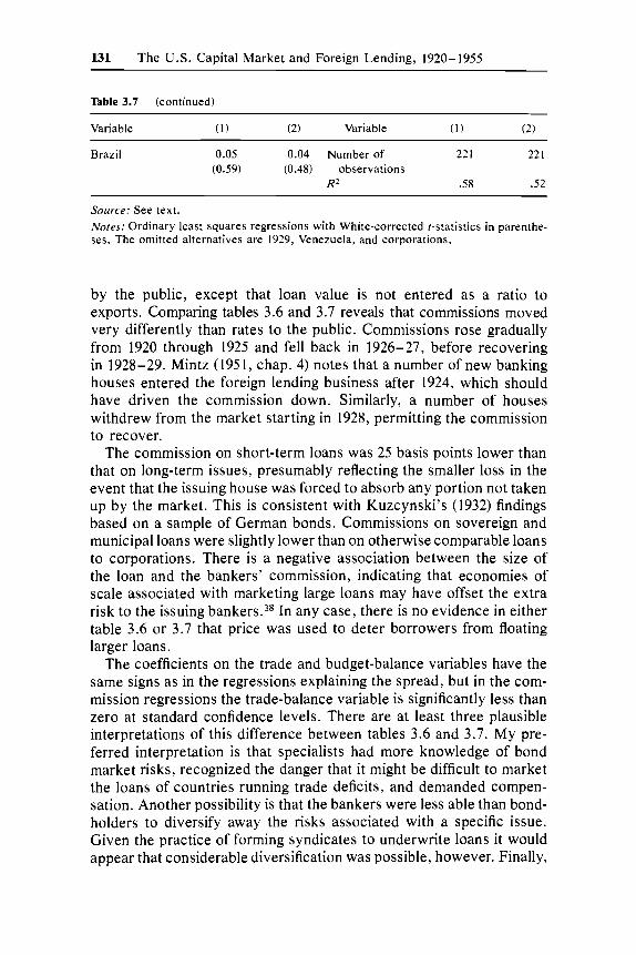
by the public, except that loan value is not entered as a ratio to exports. Comparing tables 3.6 and 3.7 reveals that commissions moved very differently than rates to the public. Commissions rose gradually from 1920 through 1925 and fell back in 1926-27, before recovering in 1928-29. Mintz (1951, chap. 4) notes that a number of new banking houses entered the foreign lending business after 1924, which should have driven the commission down. Similarly, a number of houses withdrew from the market starting in 1928, permitting the commission to recover.
The commission on short-term loans was 25 basis points lower than that on long-term issues, presumably reflecting the smaller loss in the event that the issuing house was forced to absorb any portion not taken up by the market. This is consistent with Kuzcynski’s (1932) findings based on a sample of German bonds. Commissions on sovereign and municipal loans were slightly lower than on otherwise comparable loans to corporations. There is a negative association between the size of the loan and the bankers’ commission, indicating that economies of scale associated with marketing large loans may have offset the extra risk to the issuing bankers.38 In any case, there is no evidence in either table 3.6 or 3.7 that price was used to deter borrowers from floating larger loans.
The coefficients on the trade and budget-balance variables have the same signs as in the regressions explaining the spread, but in the com- mission regressions the trade-balance variable is significantly less than zero at standard confidence levels. There are at least three plausible interpretations of this difference between tables 3.6 and 3.7. My pre- ferred interpretation is that specialists had more knowledge of bond market risks, recognized the danger that it might be difficult to market the loans of countries running trade deficits, and demanded compen- sation. Another possibility is that the bankers were less able than bond- holders to diversify away the risks associated with a specific issue. Given the practice of forming syndicates to underwrite loans it would appear that considerable diversification was possible, however. Finally,
132 Barry Eichengreen
it could be that simultaneity tending to bias the trade-balance coefficient upward (since countries charged low commissions could borrow more and hence were permitted to run large deficits) is less of a problem in table 3.7 than in table 3.6 (where a more important source of simul- taneity would arise from the ability of countries charged low interest rates to borrow more and hence to run deficits).
In sum, this analysis provides some evidence that lenders discrim- inated among potential borrowers on the basis of reputation and po- litical factors conveying information about the probability of default, but little evidence that they were responsive to current economic con- ditions in the indebted countries. Did they discriminate adequately'? One way to approach this question is to compare ex ante and ex post returns. A simple model can be used as the basis for this comparison. The expected rate of return on risky loans, i,., should exceed the risk free rate, i f , by a risk premium:
(3) i,. = i f + Su
where u is default risk so Sa is the premium on risky loans. Ex ante (of default) the return on risky loans exceeds that required:
(4) ie, unre = i r + Pa
where i,, onfr is the ex ante rate of return. The ex post return i,, differs from that required by investors by their expectational error E,
( 5 )
Substituting and solving for the ex ante return gives:
ie, post = ir + E.
If investors' expectational errors have mean zero, in a regression of
ex post on ex ante returns the constant term (, - !'sPlsif) should be
positive and the coefficient on i,, ( , n f , should be greater than unity. Using the ex ante and ex post rates of return calculated by Eichen-
green and Portes (1986) for a sample of 50 dollar bonds (national, provincial, municipal, and corporate) issued in the United States be- tween 1924 and 1930, equation (6) can be estimated, yielding:
(7) i,, = 9.00 - 120.59 i,, (0.94) (0.89)
N = 50 R2 = 0.016
with t-statistics in parentheses. Although the constant term is positive, the coefficient on i,, posr is less than unity, which is inconsistent with
133 The U.S. Capital Market and Foreign Lending, 1920-1955
the joint hypothesis of rational expectations and market efficiency. What kind of behavior does this imply? Instead of (4), posit an asset- pricing equation of the form:
(4') i,, a m = i r + (P - which can be interpreted with (Y > 0 as meaning that investors system- atically underincorporate the cost of default into the ex ante prices of those bonds most at risk. Then it is possible for the coefficient on i,, p o v ,
to be less than unity and, if (Y > P + 6, for that coefficient to be negative as in (7).
Thus, these results suggest that investors incompletely incorporated differential default risk into the spreads they demanded of foreign bor- rowers. This is surprising in light of the observed tendency (see table 3.6) of bond-market participants to demand low-risk premia of many borrowers that did not default (Scandinavian and Western European nations, members of the British Commonwealth, dependent Central American republics) and high-risk premia of many borrowers that did default (Eastern European nations, other small Latin American na- tions), since both tendencies should have given rise to a negative cor- relation between ex ante and ex post returns. But despite demanding risk premia in the appropriate instances, it nonetheless appears that they received inadequate compensation. This is particularly evident in the comparison between loans to Western European nations that per- formed well ex post and loans to Germany that performed disastrously, and between loans to Argentina and Brazil.
If default risk was imperfectly perceived at the time of issue, did bondholders recognize and act upon it subsequently? If risk-neutral investors are faced with the choice between two assets, only one of which is subject to default risk, the return on the risk-free asset should be a weighted average of the return on the other asset in instances in which default does and does not take place, where the perceived prob- ability of default is the weight. Using Y to denote the share of interest and principle lost in the event of default:
(8) ( 1 - P ) + (1 - Y ) ( 1 + i,) * P = 1 + i j-,
where P is the probability of default, and i, and if are the risky and risk-free rates of return respectively. The expected capital loss YP (default probability times percent capital loss given default) can be derived from the
(9) YP = [(i, - if)/(l + i,)].
Moody's Aaa bond rate and the yield to maturity on the sample of 50 dollar bonds, each at the end of the calendar year, are used as measures of the riskless and risky rate. Several expected losses from
(1 + i,)
134 Barry Eichengreen
0.09
0.08
0.07
0.06
0 0 5 -
004-
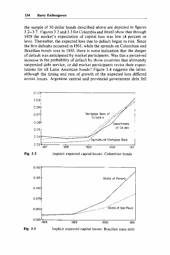
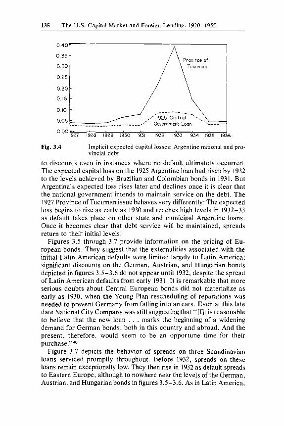
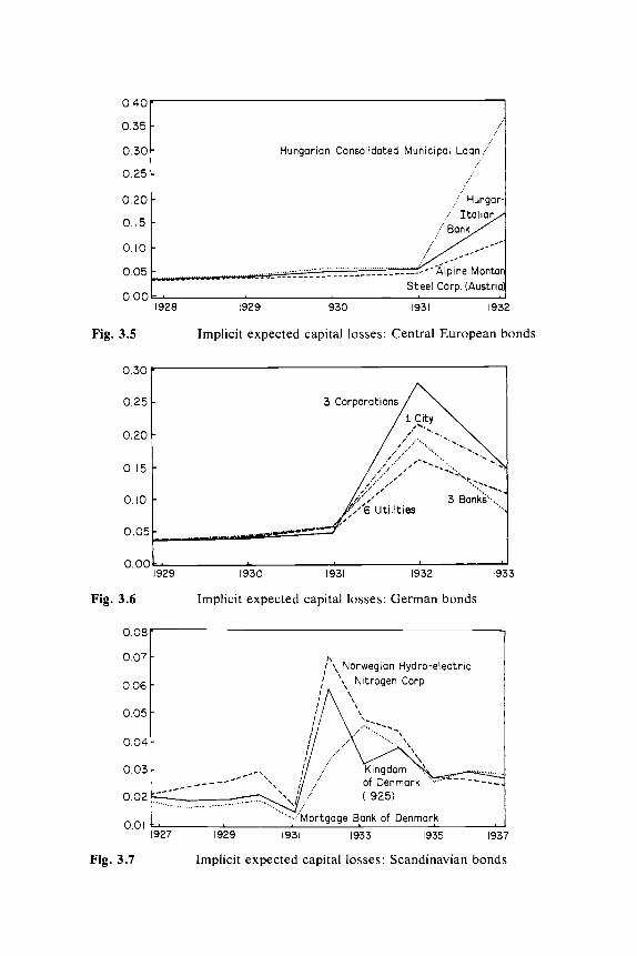
the sample of 50 dollar bonds described above are depicted in figures 3.2-3.7. Figures 3.2 and 3.3 for Colombia and Brazil show that through 1929 the market’s expectation of capital loss was low (4 percent or less). Thereafter, the expected loss due to default began to rise. Since the first defaults occurred in 193 1, while the spreads on Colombian and Brazilian bonds rose in 1930, there is some indication that the danger of default was anticipated by market participants. Was this a perceived increase in the probability of default by those countries that ultimately suspended debt service, or did market participants revise their expec- tations for all Latin American bonds? Figure 3.4 suggests the latter, although the timing and rate of growth of the expected loss differed across issues. Argentine central and provincial government debt fell
- - - -
.......................... agricu agricultural Mortgage Bank ______________- - - -----
O.15OL
0.125
0.100
0.075
0.050
0.025
Fig. 3.2 Implicit expected capital losses: Colombian bonds
-
-
-
- ...... ...................................
3
135 The U.S. Capital Market and Foreign Lending, 1920-1955
0.40b
0.35 - 0.30 - 0.25 -
0.20
0 1 5 -
010
-
-
Fig. 3.4 Implicit expected capital losses: Argentine national and pro- vincial debt
to discounts even in instances where no default ultimately occurred. The expected capital loss on the 1925 Argentine loan had risen by 1932 to the levels achieved by Brazilian and Colombian bonds in 1931. But Argentina’s expected loss rises later and declines once it is clear that the national government intends to maintain service on the debt. The 1927 Province of Tucuman issue behaves very differently: The expected loss begins to rise as early as 1930 and reaches high levels in 1932-33 as default takes place on other state and municipal Argentine loans. Once it becomes clear that debt service will be maintained, spreads return to their initial levels.
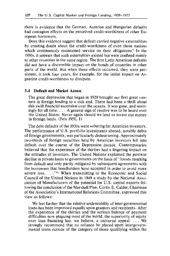
Figures 3.5 through 3.7 provide information on the pricing of Eu- ropean bonds. They suggest that the externalities associated with the initial Latin American defaults were limited largely to Latin America; significant discounts on the German, Austrian, and Hungarian bonds depicted in figures 3.5-3.6 do not appear until 1932, despite the spread of Latin American defaults from early 1931. It is remarkable that more serious doubts about Central European bonds did not materialize as early as 1930, when the Young Plan rescheduling of reparations was needed to prevent Germany from falling into arrears. Even at this late date National City Company was still suggesting that “[Ilt is reasonable to believe that the new loan . . . marks the beginning of a widening demand for German bonds, both in this country and abroad. And the present, therefore, would seem to be an opportune time for their purchase.”40
Figure 3.7 depicts the behavior of spreads on three Scandinavian loans serviced promptly throughout. Before 1932, spreads on these loans remain exceptionally low. They then rise in 1932 as default spreads to Eastern Europe, although to nowhere near the levels of the German, Austrian, and Hungarian bonds in figures 3.5-3.6. As in Latin America,
w . w r I 0.35
0.30
0.25
0.20
- - - -
Hungarian Consolidated Municipal Loan,!
:! Hungar-
. ..
1928 1929 1930 1931 1932
Fig. 3.5 Implicit expected capital losses: Central European bonds
0.ooL ' 1929 1930 1931 1932 1933
Fig. 3.6 Implicit expected capital losses: German bonds
0.08
0.07
0.06 - 0.05
0.04 -
-
-
1927 1929 1931 1933 1935 1937
Fig. 3.7 Implicit expected capital losses: Scandinavian bonds
137 The U.S. Capital Market and Foreign Lending, 1920-1955
there is evidence that the German, Austrian and Hungarian defaults had contagion effects on the perceived credit-worthiness of other Eu- ropean borrowers.
Does this evidence suggest that default carried negative externalities by creating doubt about the credit-worthiness of even those nations which continuously maintained service on their obligations? In the 1930s, it appears that such externalities existed but were confined mainly to other countries in the same region. The first Latin American defaults did not have a discernible impact on the bonds of countries in other parts of the world. But when these effects occurred, they were per- sistent; it took four years, for example, for the initial impact on Ar- gentine credit-worthiness to dissipate.
3.4 Default and Market Access
The great depression that began in 1929 brought our first great ven- ture in foreign lending to a sick end. There had been a thrill about this swift financial ascension over the oceans. It was gone, and seem- ingly for all time. . . . A general sign of resolve was to be heard over the United States: Never again should we lend or invest our money in foreign lands. (Feis 1950, 1)
The debt defaults of the 1930s were sobering for American investors. The performance of U.S. portfolio investments abroad, notably debts of foreign governments, was particularly disheartening. Approximately two-thirds of foreign securities held by American investors fell into default over the course of the Depression decade. Contemporaries believed that the experience of the thirties had a lingering impact on the attitudes of investors. The United Nations explained the postwar decline in private loans to governments on the basis of “losses resulting from default and only partly mitigated by subsequent agreements with the borrowers that bondholders have accepted in order to avoid more severe loss. . . .”41 When transmitting to the Economic and Social Council of the United Nations in 1949 a study by the National Asso- ciation of Manufacturers of the potential for U.S. capital exports fol- lowing the conclusion of the Marshall Plan, Curtis E. Calder, Chairman of the Association’s International Relations Committee, expressed this view as follows:
We feel further that the relative undesirability of inter-governmental loans has been impressed equally upon grantors and recipients. After the experience of the thirties and the serious balance of payment difficulties now plaguing most of the world, the superiority of equity over loan financing has, we believe, a universal appeal. . . . We strongly recommend that no reliance be placed upon intergovern- mental loans outside of the category of those qualifying within the

138 Barry Eichengreen
limits of the funds of Export-Import Bank and the Bank for Recon- struction and D e ~ e l o p m e n t . ~ ~
Despite a proliferation of similar statements, it is not obvious that the experience of the thirties influenced investors’ actions as well as their statements, particularly since a variety of other postwar disrup- tions might conceivably have exercised an even more powerful influ- ence over the volume and pattern of foreign lending. Moreover, any new hesitancy to extend loans to foreign governments did not have a sufficient half-life to prevent the astounding growth of sovereign debt in the 1970s. Still, it seems plausible that repercussions of the debt defaults of the 1930s were felt by the capital markets in the 1940s and 1950s. One approach to this issue is to compare U.S. foreign lending in the ten years immediately succeeding World Wars I and 11. Clearly, the second half of the 1940s and first half of the 1950s constitute a very special period in the history of the world economy, following as they do on the heels of a global conflagration. Since the years 1919-28 form an equally special period for many of the same reasons, they provide an especially useful basis for comparison. Admittedly, a study of the ten years immediately following World War I1 is not a complete analysis of the legacy-if any-of interwar debt defaults. But if no legacy of default can be discerned in the immediate postwar decade when inter- war experience was so immediate and the parallels were so extensive, it seems unlikely that such evidence could be found for subsequent years.
In comparing U.S. foreign lending in the decades immediately fol- lowing the two world wars, it is useful to distinguish three questions. First, was total U.S. foreign lending depressed in the wake of the debt defaults of the 1930s? Second, was the relative importance of direct and portfolio investment altered by the lingering effects of interwar defaults? Third, compared to countries that continuously serviced their debts, did countries that had defaulted find it more difficult to borrow abroad?
Table 3.8 summarizes the volume and composition of U.S. foreign lending in the two postwar decades. Lending from 1946 through 1955 is expressed in 1919-28 average prices. A first fact evident from table 3.8 is that U.S. capital exports actually were larger in the second postwar decade (more than three times as large at current prices, more than twice as large at constant prices). However, the difference is due almost entirely to unilateral transfers by government, notably the Mar- shall Plan. (The amount and direction of Marshall Plan aid are sum- marized in table 3.9.) Net of official transfers, U.S. foreign lending at constant prices remains almost exactly unchanged between the two postwar decades. At the most aggregated level, then, there is little
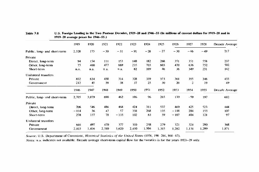
Table 3.8 U.S. Foreign Lending in the Two Postwar Decades, 1919-28 and 1946-55 (In millions of current dollars for 1919-28 and in 1919-28 average prices for 1946-55.)
1919 1920 1921 1922 1923 1924 1925 1926 1927 1928 Decade Average
Public, long- and short-term 2,328 175 -30 -31 -91 -28 ~ - 2 7 -30 -46 -49 217
Private Direct, long-term 94 I54 111 153 I 48 182 268 35 1 35 1 558 237 Other, long-term 75 400 477 669 235 703 603 470 636 752 502 Short-term n.a. n.a. n.a. n.a. 82 I 0 9 46 36 349 231 142
Unilateral transfers Private 832 634 450 314 328 339 373 361 355 346 433 Government 212 45 59 38 37 25 30 20 2 19 49
1946 1947 1948 1949 1950 1951 1952 1953 1954 1955 Decade Average
Public, long- and short-term 2,705 3,079 690 462 106 96 265 139 -59 197 682
Private Direct, long-term Other, long-term Short-term
206 546 486 468 424 311 537 469 425 523 444 114 36 47 57 338 268 135 - 118 204 153 I07 278 I37 78 -133 102 63 59 - I07 404 121 97
Unilateral transfers Private 603 497 470 377 310 258 279 32 I 32 I 290 368 Government 2,015 1,416 2,580 3,620 2,430 1,904 1,315 1,262 1,131 1,299 1,871
Source: U.S. Department of Commerce, Historical Statistics of the United States (1976, 198-201, 866-67). Notcs: n.a. indicates not available. Decade average short-term capital flow for the twenties is for the years 1923-28 only.
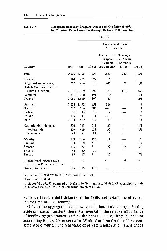
140 Barry Eichengreen
Table 3.9 European Recovery Program Direct and Conditional Aid, by Country: From Inception through 30 June 1951 ($million)
Grants
Conditional upon Aid Extended
Under Intra Through European European Payments Payments
Country Total Total Direct Agreement" Union
Total 10,260 9,128 7,537 1,355 236
Austria 492 492 488 5 Belgium-Luxembourg 537 484 8 447 29 British Commonwealth:
United Kingdom 2,675 2.329 1,799 380 150 Denmark 231 200 191 9 France 2,060 1,869 1,807 61
Germany 1,174 1,172 953 219 - Greece 387 386 386 - - Iceland 17 13 10 4 Ireland 139 I I I I Italy 1,034 959 873 86 -
Netherlands-Indonesia 893 743 711 32 -
-
- -
- - -
- Netherlands 809 659 628 30 Indonesia 84 84 83 1
Norway 199 164 153 I I Portugal 33 8 * 8 Sweden 103 82 * 77 5 Trieste 30 30 30 - - Turkey 89 17 * 17
International organization: 51 51 - - 51
Unclassified areas 116 116 116 - -
- -
-
-
European Payments Union
Credits
1,132
- 52
346 31
191
2 1 3
128 74
151 151 -
25 35 20
71
-
-
-
Source: U . S . Department of Commerce (1952, 60). *Less than $500,000. "Includes $3,500,000 extended by Iceland to Germany and $3,081,000 extended by Italy to Trieste outside of the intra-European payments plan.
evidence that the debt defaults of the 1930s had a damping effect on the volume of U.S. lending.
Only at the aggregate level, however, is there little change. Putting aside unilateral transfers, there is a reversal in the relative importance of lending by government and by the private sector, the public sector accounting forjust 20 percent after World War I but for fully 51 percent after World War 11. The real value of private lending at constant prices
141 The U.S . Capital Market and Foreign Lending, 1920-1955
(long- and short-term combined) fell by nearly one third between the post-World War I and post-World War I1 decades. Within private lend- ing, there are equally far-reaching changes in composition. While the share of short-term capital in U.S. private lending remains more or less unchanged, the relative importance of direct and portfolio invest- ment is reversed. Where portfolio investment was more than double direct investment in the decade following World War I, it was less than a quarter of direct investment in the decade following World War 11. Although there are other reasons why reliance on direct investment might have increased after World War 11-such as the standard pre- sumption that direct investment is relatively advantageous for firms engaged in the manufacture of goods produced with firm-specific tech- nical knowledge, a type of production that tended to grow more im- portant in international transactions as the century progressed-it seems implausible that these slowly-evolving factors rather than the reper- cussions of default were mainly responsible for the very dramatic rise in direct investment after 1945. Because of both the fall in the real value of private lending and the declining share of portfolio investment, the real value of the latter fell most dramatically between decades, by more than 80 percent. Overall, there was a dramatic decline in the willingness of Americans to accumulate portfolio investments abroad, precisely what one would expect had purchasers been deterred by defaults on foreign bonds.
While the United States was far and away the leading capital exporter of the post-World War I1 period, she had not been so dominant after World War I. In the period 1924-27, when U.S. capital exports fluc- tuated in the range of $1 .241 .6 billion per annum, total capital exports of the industrial countries reached $2 billion annually and more.43 It is noteworthy, therefore, that private capital exports of other industrial countries fell even more dramatically between the two postwar decades than did the capital exports of the United States. New issues for over- seas account floated in London in the period 1947-52 amounted to f45 million per annum, less than 50 percent of the current-price value of the period 1920-25. Meanwhile, British investors steadily repatriated their foreign funds between 1946 and 1951. The nominal value of the overseas investments of U.K. residents in the form of securities quoted on the London Stock Exchange declined by f432 million.44 The outflow of private capital from France over the period 1946-52 is estimated to have approached a total of $ 1 billion; in contrast, in the period 1920- 26 the total outflow (excluding gold) had been more than $3.5 billion.45
Consistent country data on the extent of foreign borrowing after World War I1 are notoriously difficult to obtain. Fortunately, courtesy of Avramovic’s (1958) massive study, reasonably consistent data on stocks of debt at three points in time are available for 36 countries. As
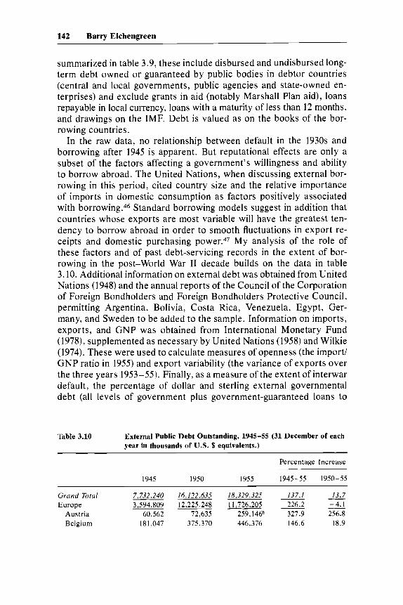
142 Barry Eichengreen
summarized in table 3.9, these include disbursed and undisbursed long- term debt owned or guaranteed by public bodies in debtor countries (central and local governments, public agencies and state-owned en- terprises) and exclude grants in aid (notably Marshall Plan aid), loans repayable in local currency, loans with a maturity of less than 12 months, and drawings on the IMF. Debt is valued as on the books of the bor- rowing countries.
In the raw data, no relationship between default in the 1930s and borrowing after 1945 is apparent. But reputational effects are only a subset of the factors affecting a government’s willingness and ability to borrow abroad. The United Nations, when discussing external bor- rowing in this period, cited country size and the relative importance of imports in domestic consumption as factors positively associated with b o r r o ~ i n g . ~ ~ Standard borrowing models suggest in addition that countries whose exports are most variable will have the greatest ten- dency to borrow abroad in order to smooth fluctuations in export re- ceipts and domestic purchasing power.47 My analysis of the role of these factors and of past debt-servicing records in the extent of bor- rowing in the post-World War I1 decade builds on the data in table 3.10. Additional information on external debt was obtained from United Nations (1948) and the annual reports of the Council of the Corporation of Foreign Bondholders and Foreign Bondholders Protective Council, permitting Argentina, Bolivia, Costa Rica, Venezuela, Egypt, Ger- many, and Sweden to be added to the sample. Information on imports, exports, and GNP was obtained from International Monetary Fund (1978), supplemented as necessary by United Nations (1958) and Wilkie (1974). These were used to calculate measures of openness (the import/ GNP ratio in 1955) and export variability (the variance of exports over the three years 1953-55). Finally, as a measure of the extent of interwar default, the percentage of dollar and sterling external governmental debt (all levels of government plus government-guaranteed loans to
Table 3.10 External Public Debt Outstanding, 1945-55 (31 December of each year in thousands of U.S. $ equivalents.)
Percentage Increase
1945 1950 I955 1945-55 1950-55
Grund Torul 7,732,240 16,122,635 18,329,325 137.1 13.7
Austria 60,562 72,635 259,146b 327.9 256.8 Belgium 18 1,047 375,370 446.376 146.6 18.9
Europe 3,594,809 12,225,248 11,726,205 226.2 -4.1
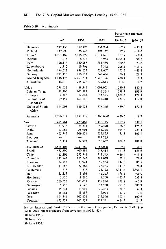
143 The U.S. Capital Market and Foreign Lending, 1920-1955
Table 3.10 (continued)
1945 1950
Percentage Increase
1955 1945-55 1950-55
Denmark Finland France Iceland Italy Luxembourg Netherlands Norway United Kingdom Yugoslavia
Africa Belgian Congo Ethiopia Federation of
Rhodesia Union of South
Africa
Australia
Asia Ceylon India Japan Pakistan Thailand
Latin America Brazil Chile Colombia Ecuador El Salvador Guatemala Haiti Honduras Mexico Nicaragua Panama Paraguay Peru Uruguay
272, I35 147,998
1,267, I82 1,216
126,116 5,310
194,612 222,456
1,116,175 n.a.
296,052 79,206
2,786 69, I57
144,903
1,760,514
495,764 37,918 47,467
402,945
7,434
1,585,102 432,699 425,892 171,447 24,222 13,383
878 15,155 5,430
200,577 5,776
15,641 15,781
104,842 153,379
-
389,493 326,742
2,906,297 8,633
550,268 19,502
939,625 286,523
6,061,234 288,926”
438,548 107,719 12,000
169,806
149,023
I ,288,118
429,461 26,345 58,998
309, I21
34,997
1,741,260 409,389 355,346 157,545 3 1,944 22,367
378 8,296 1,260
509,099 4,640
13,000 15,287
107,176 105,533
-
25 1,984 292,177
2,631,671 16,965
681,450 17,342
53 1,607 347,476
5,920,196 329,815
1,093,903 3 1 6,564c 32,583
368,410
376,346
1 ,400,084b
1,426,125 59,470
486,378 627,855 181,785 70,637
2,683,008 1,046,4 14
313,543 28 1,079
59,254 28,263 21,172 42,225 4,200
478,944 22,730 20,463 17,974
2 15,366 131,381
-7.4 97.4
107.7 1,295.1
440.3 226.6 173.2 56.2
430.4 n.a.
269.5 299.7
1,069.5 432.7
459.7
- 20.5
187.7 56.8
924.7 55.8
850.2
69.3 141.8 - 26.4
63.9 144.6 111.2
2,311.4 178.6
-22.7 138.8 293.5 30.8 13.9
105.4 - 14.3
-
- 35.3 - 10.6 - 9.4 96.5 23.8
- 11.1 -43.4
21.3 -2.3 14.2
149.4 193.9 171.5 117.0
152.5
8.7
232.1 125.7 724.4 103.1
101.8
54. I 155.6
78.4 85.5 26.4
5,501.1 409.0 233.3 - 5.9 389.9 57.4 17.6
100.9 24.5
-
-
-11.8
Source: International Bank of Reconstruction and Development, Economic Staff, Sta- tistics Division: reproduced from Avramovic (1958, 163). “30 June 1951. b30 June 1955. ‘30 June 1956.
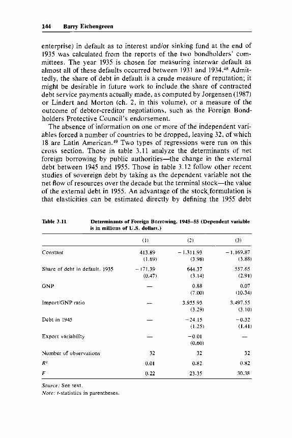
144 Barry Eichengreen
enterprise) in default as to interest and/or sinking fund at the end of 1935 was calculated from the reports of the two bondholders’ com- mittees. The year 1935 is chosen for measuring interwar default as almost all of these defaults occurred between 1931 and 1934.48 Admit- tedly, the share of debt in default is a crude measure of reputation; it might be desirable in future work to include the share of contracted debt service payments actually made, as computed by Jorgensen (1987) or Lindert and Morton (ch. 2, in this volume), or a measure of the outcome of debtor-creditor negotiations, such as the Foreign Bond- holders Protective Council’s endorsement.
The absence of information on one or more of the independent vari- ables forced a number of countries to be dropped, leaving 32, of which 18 are Latin Ame~ican .~9 Two types of regressions were run on this cross section. Those in table 3.11 analyze the determinants of net foreign borrowing by public authorities-the change in the external debt between 1945 and 1955. Those in table 3.12 follow other recent studies of sovereign debt by taking as the dependent variable not the net flow of resources over the decade but the terminal stock-the value of the external debt in 1955. An advantage of the stock-formulation is that elasticities can be estimated directly by defining the 1955 debt
Table 3.11 Determinants of Foreign Borrowing, 1945-55 (Dependent variable is in millions of U.S. dollars.)
Constant 413.89 -
(1.69) I ,311.93 -
(3.98) 1,169.87
(3.88)
Share of debt in default, 1935 - 171.39 644.37 557.65 (0.47) (3.14) (2.91)
GNP
IrnportiGNP ratio
- 0.88 0.07 (7.00) (10.34)
- 3,955.93 3,497.55 (3.29) (3.10)
- Debt in 1945 -
Export variability
24.15 - 0.32 (1.25) (1.41)
- -0.01 - (0.60)
Number of observations 32 32 32
R2 0.01 0.82 0.82
F 0.22 23.35 30.38
Source: See text. Nore; t-statistics in parentheses.
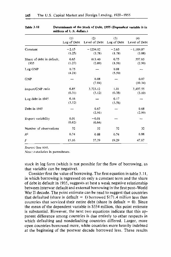
145 The U.S. Capital Market and Foreign Lending, 1920-1955
Table 3.12 Determinants of the Stock of Debt, 1955 (Dependent variable is in millions of U.S. dollars.)
(1) (2) (3) (4) Log of Debt Level of Debt Log of Debt Level of Debt
Constant
Share of debt in default, 1935
Log GNP
GNP
ImportiGNP ratio
Log debt in 1945
Debt in 1945
Export variability
Number of observations
R2
F
-2.15 (1.25)
0.65 (1.27)
0.75 (4.21)
0.85 (0.31)
0.16 (3.52)
-
0.01 (0.62)
32
0.74
15.16
-1254.12 (3.78)
613.40 (2.89)
0.08 (7.04)
3,723.12 (3.12)
0.67 (2.91)
-0.01 (0.64)
32
0.88
37.39
- - 2.65 (1.78)
0.75 (1.56)
0.81 (5.50)
1.01 (0.38)
0.17 (3.56)
32
0.74
19.29
1,169.87 (3.88)
557.65 (2.90)
0.07 (10.34)
3,497.55 (3.10)
0.68 (2.99)
32
0.88
47.67
Source: See text. Note: r-statistics in parentheses.
stock in log form (which is not possible for the flow of borrowing, as that variable can be negative).
Consider first the value of borrowing. The first equation in table 3.11, in which borrowing is regressed on only a constant term and the share of debt in default in 1935, suggests at best a weak negative relationship between interwar default and external borrowing in the first post-World War I1 decade. The point estimate can be read to suggest that countries that defaulted (share in default = 1) borrowed $171.4 million less than countries that serviced their entire debt (share in default = 0). Since the mean of the dependent variable is $334 million, this point estimate is substantial. However, the next two equations indicate that this ap- parent difference among countries is due entirely to other respects in which defaulting and nondefaulting countries differed. Larger, more open countries borrowed more, while countries more heavily indebted at the beginning of the postwar decade borrowed less. These results
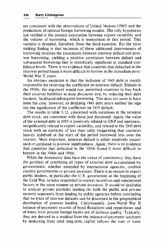
146 Barry Eichengreen
are consistent with the observations of United Nations (1965) and the predictions of optimal foreign borrowing models. The only hypothesis not verified is the posited association between export variability and the volume of borrowing, which is nonexistent in this period. This variable is dropped, therefore, from the third equation. But the most striking finding is that inclusion of these additional determinants of borrowing reverses the association between interwar default and post- war borrowing, yielding a positive correlation between default and subsequent borrowing that is statistically significant at standard con- fidence levels. There is no evidence that countries that defaulted in the interwar period found it more difficult to borrow in the immediate post- World War I1 years.
An obvious suspicion is that the inclusion of 1945 debt is mainly responsible for reversing the coefficient on interwar default. Default in the 1930s, the argument would run, permitted countries to buy back their external liabilities at deep discounts and, by reducing their debt burdens, facilitated subsequent borrowing. This does not seem to have been the case, however, as dropping 1945 debt alters neither the sign nor the significance of the coefficient on 1935 default.
The results in table 3.12, concerned with variations in the terminal debt stock, are consistent with those just discussed. Again, the value of the external debt in 1955 is positively related to GNP and openness, insignificantly related to export variability, and related to the 1945 debt stock with an elasticity of less than unity (suggesting that countries heavily indebted at the start of the period borrowed less over the interim). Most important, interwar default is either positively associ- ated or unrelated to postwar indebtedness. Again, there is no evidence that countries that defaulted in the 1930s found it more difficult to borrow in the 1940s and 1950s.
While the Avramovic data have the virtue of consistency, they have the problem of combining all types of external debt accumulated by governments, whether extended by international agencies, creditor country governments or private investors. There is no reason to expect public lenders, in particular the U.S. government at the beginning of the Cold War, to have responded to market incentives and reputational factors in the same manner as private investors. It would be desirable to analyze private portfolio lending (to both the public and private sectors) separately from lending by public agencies before concluding that no trace of interwar defaults can be discerned in the geographical distribution of postwar lending. Unfortunately, post-World War I1 balance-of-payments records of bond floatations and repurchases and of loans from private foreign banks are of dubious quality. Typically, they are derived as a residual from the balance-of-payments accounts by deducting from total long-term capital inflows the sum of loans
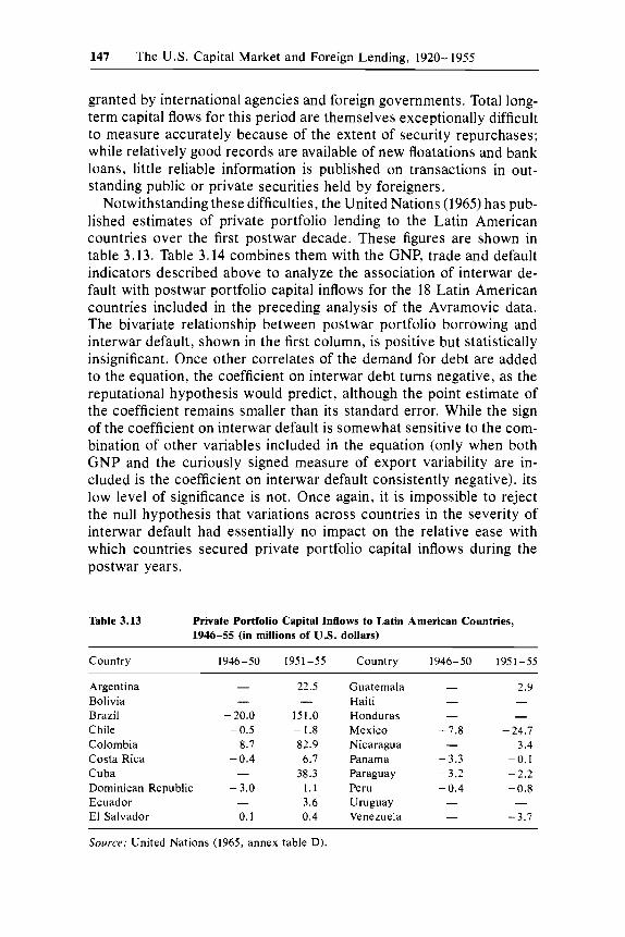
147 The U.S. Capital Market and Foreign Lending, 1920-1955
granted by international agencies and foreign governments. Total long- term capital flows for this period are themselves exceptionally difficult to measure accurately because of the extent of security repurchases; while relatively good records are available of new floatations and bank loans, little reliable information is published on transactions in out- standing public or private securities held by foreigners.
Notwithstanding these difficulties, the United Nations (1965) has pub- lished estimates of private portfolio lending to the Latin American countries over the first postwar decade. These figures are shown in table 3 .13 . Table 3.14 combines them with the GNP, trade and default indicators described above to analyze the association of interwar de- fault with postwar portfolio capital inflows for the 18 Latin American countries included in the preceding analysis of the Avramovic data. The bivariate relationship between postwar portfolio borrowing and interwar default, shown in the first column, is positive but statistically insignificant. Once other correlates of the demand for debt are added to the equation, the coefficient on interwar debt turns negative, as the reputational hypothesis would predict, although the point estimate of the coefficient remains smaller than its standard error. While the sign of the coefficient on interwar default is somewhat sensitive to the com- bination of other variables included in the equation (only when both GNP and the curiously signed measure of export variability are in- cluded is the coefficient on interwar default consistently negative), its low level of significance is not. Once again, it is impossible to reject the null hypothesis that variations across countries in the severity of interwar default had essentially no impact on the relative ease with which countries secured private portfolio capital inflows during the postwar years.
Table 3.13 Private Portfolio Capital Inflows to Latin American Countries, 1946-55 (in millions of U.S. dollars)
Country 1946-50 1951-55 Country 1946-50 1951-55
Argentina Bolivia Brazil Chile Colombia Costa Rica Cuba Dominican Republic Ecuador El Salvador
- 22.5
- 20.0 151.0
8.7 82.9 -0.4 6.7 - 38.3
- 3.0 1.1 - 3.6 0.1 0.4
- -
- 0.5 - 1.8
Guatemala Haiti Honduras Mexico Nicaragua Panama Paraguay Peru Uruguay Venezuela
- -
-7.8
-3.3 -3.2 - 0.4
-
-
2.9 - -
- 24.7 3.4
-0.1 -2.2 -0.8
-3.7 -
Source: United Nations (1965, annex table D).
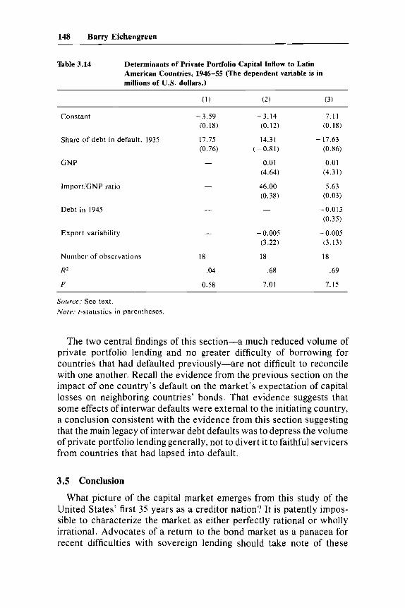
148 Barry Eichengreen
Table 3.14 Determinants of Private Portfolio Capital Inflow to Latin American Countries, 1946-55 (The dependent variable is in millions of U.S. dollars.)
Constant
Share of debt in default, 1935
G N P
Impor tGNP ratio
Debt in 1945
Export variability
Number of observations
R2
F
- 3.59 (0.18)
17.75 (0.76)
18
.04
0.58
-3.14 (0.12)
- 14.31 (-0.81)
0.01 (4.64)
46.00 (0.38)
-0.005 ( 3 . 2 2 )
18
.68
7.01
7.11 (0.18)
- 17.63 (0.86)
0.01 (4.31)
5.63 (0.03)
-0.013 (0.35)
- 0.005 (3.13)
18
.69
7.15
Source: See text. Note: t-statistics in parentheses.
The two central findings of this section-a much reduced volume of private portfolio lending and no greater difficulty of borrowing for countries that had defaulted previously-are not difficult to reconcile with one another. Recall the evidence from the previous section on the impact of one country’s default on the market’s expectation of capital losses on neighboring countries’ bonds. That evidence suggests that some effects of interwar defaults were external to the initiating country, a conclusion consistent with the evidence from this section suggesting that the main legacy of interwar debt defaults was to depress the volume of private portfolio lending generally, not to divert it to faithful servicers from countries that had lapsed into default.
3.5 Conclusion
What picture of the capital market emerges from this study of the United States’ first 35 years as a creditor nation? It is patently impos- sible to characterize the market as either perfectly rational or wholly irrational. Advocates of a return to the bond market as a panacea for recent difficulties with sovereign lending should take note of these
149 The U.S. Capital Market and Foreign Lending, 1920-1955
conclusions. While switching back from bank loans to the bond market may divert some of the risk shouldered by creditor-country banking systems, bond market participants have shown no greater facility than bank loan officers historically in distinguishing good credit risks from bad. Nor were bond markets any more successful in smoothing the flow of capital to developing-country debtors.
What picture of the legacy of default for the subsequent behavior of the markets emerges from this study of the last complete debt cycle? Recent theoretical studies of sovereign lending in the presence of po- tential default have posited the existence of a default penalty, p , usually interpreted as the costs of inferior access to international capital mar- kets in the wake of default. The finding that, compared to countries that maintained debt service throughout, countries that lapsed into default in the 1930s were no less able to borrow in the 1940s and 1950s is difficult to reconcile with this simple view. If there were costs of default, they did not take the form of differential credit-market access in the first postwar decade. But this does not imply that default was costless. Evidence from bond prices in the 1930s and from the volume and composition of lending in the 1940s-1950s suggests that at least some of the costs of default spilled over among debtor countries. These costs took the form of reduced access to private portfolio capital flows for defaulting and nondefaulting countries alike.
To say that default had costs is not to say that it was necessarily welfare reducing. It may also have had benefits in the form of the spur to growth and adjustment provided by a lightened debt burden. Com- parisons of economic growth and structural change in defaulting and nondefaulting countries will be needed before welfare conclusions can be drawn. But the fact that a substantial share of the costs were external to the individual country indicates that there may be gains to debtors from coordinating their decisions, whether or not that decision is to maintain service on their external debts.
Notes
I . Computed from Lewis (1938, 445). 2. If war debts are added to U.S. foreign assets, the U.S. net creditor position
3. For figures, see Eichengreen (1986). 4. Fraga (1986, sec. 2). Some have suggested that the German authorities
consciously wished to build up commercial liabilities as a way of impressing on American creditors the impossibility of making good both commercial and reparations obligations. For a discussion, see McNeil (1986).
in 1919 exceeds $12 billion.
5. See Lipsey (1988).
150 Barry Eichengreen
6. Foreign bond yields are annual averages, from Lary (1943, 204). Moody’s Baa yields are from the U.S. Department of Commerce, Survey of Current Business (1937, 19). The value of total publicly offered foreign securities pur- chased in the United States (including refunding to Americans) is from Dickens (1932, 8). The picture for the other major creditor country, Britain, looks broadly similar although the fluctuations in lending are considerably damped; see Eichengreen and Portes (1986, sec. 2).
7. It is conceivable, of course, that the lending series is traced out not by movements of the supply curve along a stable demand curve but by shifts in borrowers’ demand (down in 1923, up starting in 1924, and down after 1928). I argue, however, that demand remained relatively stable at high levels through- out the decade and that changes in quantities reflected mainly shifts in supply.
8. Lewis’s (1938, 370) estimates of yields to maturity are 5.3 percent for 1915-April 1917 and 6.7 percent for 1922-24. The 1920 Belgian loan illustrates the difficulties encountered by borrowers at the beginning of the decade. It has been argued that Belgium managed to obtain these funds only because U.S. commercial banks had a special stake in the country. The banks had previously extended Belgium short-term credits in the amount of $50 million to purchase wheat and other essential commodities. Because of a deterioration in the country’s external position, it quickly became evident that the govern- ment was in no position to repay. The authorities therefore approached the bankers, who agreed to float $50 million worth of 25-year bonds. The terms were highly favorable to investors: the bonds bore a nominal interest rate of 7.5 percent and were callable only at 115. Yet “the subscription books were kept open for three days, a very unusual procedure; every resource the bankers could command was used to induce subscription . . . .” Only after having taken these exceptional steps was the loan successfully floated. See Swan (1928), from which the above quotation is drawn.
9. As Lawrence Speaker wrote in 1924 (93), “From the political standpoint, Europe today presents a very uncertain outlook. Since most of Eastern Europe is in the hands of the radical socialists whose views on capital are quite in- compatible with those held here, since Central Europe is threatened with po- litical as well as economic breakdown, and the nations of Western Europe are torn apart by contending political influences, a policy of extreme caution in making investments in Europe seems highly advisable. It is possible that some of these countries, in their dire necessity, may be drawn to the confiscation of private property as well as wholesale repudiation of their internal debts. . . . Such tendencies on the part of governments are not a t all conducive to the stability and soundness of investments.”
10. The Economist (5 July 1924) described the return as follows, “The yield, allowing for redemption in twenty years, works out at approximately f 8 16s. per cent. This is a high yield and indicates to some extent the measure of risk involved.”
11. Costigliola (1976, 490) suggests that the Fed took this action in order to render investment in the Dawes loan more attractive.
12. Stoddard (1932, 43). 13. Stoddard (1932, 43). 14. Cleveland and Huertas (1985, 135). 15. When in 1919 National City Bank opened its Lima branch, for example,
the president of Peru offered the National City Company the opportunity to become the nation’s investment banker (Phelps 1927,211 ; Cleveland and Huer- tas 1985, 177; see also Carosso 1970).
16. Cleveland and Huertas (1985, 137).
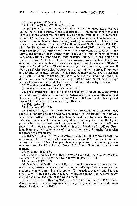
151 The U.S. Capital Market and Foreign Lending, 1920-1955
17. See Speaker (1924, chap. 2). 18. Robinson (1926, 327-28 and passim). 19. Both types of tales are too well known to require elaboration here. On
selling the foreign borrower, one Department of Commerce expert told the Senate Finance Committee of a time at which there were at least 29 represen- tatives of American investment banking firms in Colombia seeking to negotiate various loans. A Bavarian town initially wishing to borrow $125,000 was con- vinced to commission an issue of $3 million instead (U.S. Senate 1932, 845- 48, 1279-80). On selling the small investor, Stoddard (1932, 106) writes, “Up to the slump of 1920, these new clients sought the branch-offices. After the slump, the branch-offices sought them. They did it through hosts of young salesmen, carefully schooled in ‘high pressure’ methods of breaking down ‘sales resistance.’ The keynote was pressure-all down the line. The home office kept the branch-offices ‘on their toes’ by a stream of phone-calls, ‘flashes,’ ‘pep-wires,’ and so forth. The branch managers kept the young salesmen all ‘burned up’ with ‘pep-talks,’ bonuses, and threats of getting fired. Everybody in authority demanded ‘results’; which meant, more sales. Every salesman must sell his ‘quota.’ What he sold, how he sold it, and whom he sold it to, did not much matter. Verily, business had got into banking; or, rather, ‘banking,’ in the old sense of the word, had been kicked out of doors by business.”
20. Cleveland and Huertas (1985, 177). 21. Madden, Nadler, and Sauvain (1937, 222). 22. The significance of this moral hazard problem is impossible to determine
in the absence of detailed study of the operations of particular affiliates. But it is worth noting in this connection that White (1986) has found little empirical support for other criticisms of security affiliates.
23. Feis (1950, 13). 24. Brandes (1962, 128). 25. Dulles (1926, 35-37). There were also objections on other occasions,
such as a loan for a Czech brewery, presumably on the grounds that this was inconsistent with a U.S. policy of Prohibition, and for a Brazilian coffee valori- zation scheme and a German potash syndicate, on the grounds that the higher prices which would result would be harmful to U.S. consumers. (Both bor- rowers ultimately succeeded in obtaining funds in London.) In addition, Pres- ident Harding urged his secretary of state to discourage U.S. lending for foreign purchases of armaments.
26. Brandes (1962, 177-78) and Angel1 (1933, 101-2). France managed to circumvent U . S . restrictions to some extent before 1928. For example, Ivar Kreuger’s Swedish Match Company loaned large sums to the French govern- ment soon after its U.S. subsidiary floated $50 million of bonds on the American market.
27. Williams (1929, 95). 28. Cited in Brandes (1962, 186). Extracts from the whole series of State
29. Brandes (1962, 188). 30. Madden and Nadler (1929, 83), for example, in a manual on securities
investment, instruct investors to consider trade and budget balances and natural resource endowments. (See also pp. 96-97). Madden, Nadler, and Sauvain (1937, 207) mention the trade balance, the budget balance, the position of the central bank, and the debt of the government.
31. Consistent with this hypothesis, Eichengreen and Portes (1986) found that government budget surpluses were negatively associated with the inci- dence of default in the 1930s.
Department letters are provided by Kuczynski (1932, 10- 11).
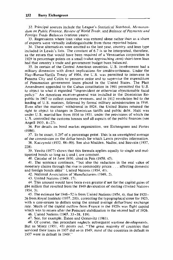
152 Barry Eichengreen
32. Principal sources include the League’s Statistical Yearbook, Mernoran- durn on Public Finance, Review of World Trade, and Balance of Payments and Foreign Trade Balances (various years).
33. Regressions where loan value was entered alone rather than as a share of exports were virtually indistinguishable from those reported below.
34. These alternatives were omitted as the last year, country, and loan type included in Lewis’s lists. The constant of 6.7 is to be interpreted, therefore, as the return that would have been required of a Venezuelan corporation in 1929 in percentage points on a small (value approaching zero) short-term loan had that country’s trade and government budget been balanced.
35. In certain of the Central American countries, U.S. involvement had a military dimension with direct implications for creditworthiness. Under the Hay-Bunau-Varilla Treaty of 1904, the U.S. was permitted to intervene in Panama City and Colon to preserve order and to supervise the expenditure of Panamanian government loans placed in the United States. The Platt Amendment appended to the Cuban constitution in 1901 permitted the U.S. to object to what it regarded “improvident or otherwise objectionable fiscal policy.” An American receiver-general was installed in the Dominican Re- public in 1907 to collect customs revenues, and in 1912 revolution led to the landing of U.S. marines, followed by formal military administration in 1916. Even after the marines’ withdrawal in 1924, the United States retained the right to object to changes in Dominican tariffs and public debt. Haiti was under U.S. martial law from 1916 to 1931, under the provisions of which the U.S . controlled the customs houses and all aspects of the public finances (see Angel1 1933, 8-27).
36. For details on bond market organization, see Eichengreen and Portes (1 986).
37. To be exact, 0.297 of a percentage point. This is an unweighted average of the commission on the dollar bonds for which Lewis provides information.
38. Kuczynski (1932, 88-89). See also Madden, Nadler, and Sauvain (1937, 228).
39. Yawitz (1977) shows that this formula applies equally to single and mul- tiperiod bonds so long as if and i, are constant.
40. Circular of 14 June 1930, cited in Feis (1950, 45). 41. The sentence continues, “but also the reduction in the real value of
monetary claims through the rise in commodity prices . . . affecting domestic and foreign bonds alike” United Nations (1954, 41).
42. National Association of Manufacturers (1949, 2). 43. United Nations (1949, 17). 44. This amount would have been even greater if not for the capital gains of
f 8 4 million that resulted from the 1949 devaluation of sterling (United Nations 1954, 3).
45. The estimate for 1946-52 is from United Nations (1954,4), that for 1920- 26 from Royal Institute (1937,200), correcting the typographical error for 1923, with a conversion to dollars using the annual average dollarlfranc exchange rate. Much of the capital outflow from France in the 1920s was flight capital which was to return after the Poincare stabilization in the second half of 1926.
46. United Nations (1965, 33-38, 119). 47. See, for example, Eaton and Gersovitz (1981). 48. Of course, this procedure neglects subsequent wartime developments.
But as Mintz (1951, 43) points out, “The great majority of countries that serviced their loans in 1937 did so in 1949; most of the countries in default in 1937 were in default in 1949.”
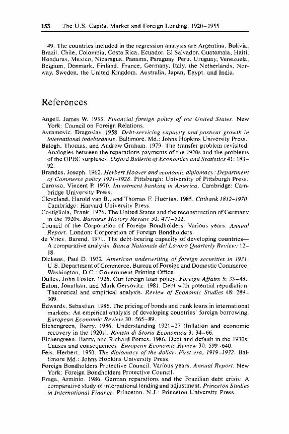
153 The U.S. Capital Market and Foreign Lending, 1920-1955
49. The countries included in the regression analysis are Argentina, Bolivia, Brazil, Chile, Colombia, Costa Rica, Ecuador, El Salvador, Guatemala, Haiti, Honduras, Mexico, Nicaragua, Panama, Paraguay, Peru, Uruguay, Venezuela, Belgium, Denmark, Finland, France, Germany, Italy, the Netherlands, Nor- way, Sweden, the United Kingdom, Australia, Japan, Egypt, and India.
References
Angell, James W. 1933. Financial foreign policy of the United States. New York: Council on Foreign Relations.
Avramovic, Dragoslav. 1958. Debt-servicing capacity and postwar growth in international indebtedness. Baltimore, Md.: Johns Hopkins University Press.
Balogh, Thomas, and Andrew Graham. 1979. The transfer problem revisited: Analogies between the reparations payments of the 1920s and the problems of the OPEC surpluses. Oxford Bulletin of Economics and Statistics 41: 183- 92.
Brandes, Joseph. 1962. Herbert Hoover and economic diplomacy: Department of Commerce policy 1921-1928. Pittsburgh: University of Pittsburgh Press.
Carosso, Vincent P. 1970. Investment banking in America. Cambridge: Cam- bridge University Press.
Cleveland, Harold van B., and Thomas F. Huertas. 1985. Citibank 1812-1970. Cambridge: Harvard University Press.
Costigliola, Frank. 1976. The United States and the reconstruction of Germany in the 1920s. Business History Review 50: 477-502.
Council of the Corporation of Foreign Bondholders. Various years. Annual Report. London: Corporation of Foreign Bondholders.
de Vries, Barend. 1971. The debt-bearing capacity of developing countries- A comparative analysis. Banca Nationale del Lavoro Quarterly Review: 12- 18.
Dickens, Paul D. 1932. American underwriting of foreign securities in 1931. U.S. Department of Commerce, Bureau of Foreign and Domestic Commerce. Washington, D.C.: Government Printing Office.
Dulles, John Foster. 1926. Our foreign loan policy. Foreign Affairs 5: 33-48. Eaton, Jonathan, and Mark Gersovitz. 1981. Debt with potential repudiation:
Theoretical and empirical analysis. Review of Economic Studies 48: 289- 309.
Edwards, Sebastian. 1986. The pricing of bonds and bank loans in international markets: An empirical analysis of developing countries’ foreign borrowing. European Economic Review 30: 565-89.
Eichengreen, Barry. 1986. Understanding 1921 -27 (Inflation and economic recovery in the 1920s). Rivista di Storiu Economica 3: 34-66.
Eichengreen, Barry, and Richard Portes. 1986. Debt and default in the 1930s: Causes and consequences. European Economic Review 30: 599-640.
Feis, Herbert. 1950. The diplomacy of the dollar: First era, 1919-1932. Bal- timore Md.: Johns Hopkins University Press.
Foreign Bondholders Protective Council. Various years. Annual Report. New York: Foreign Bondholders Protective Council.
Fraga, Arminio. 1986. German reparations and the Brazilian debt crisis: A comparative study of international lending and adjustment. Princeton Studies in International Finance. Princeton, N.J.: Princeton University Press.
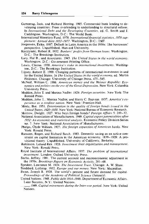
154 Barry Eichengreen
Guttentag, Jack, and Richard Herring. 1985. Commercial bank lending to de- veloping countries: From overlending to underlending to structural reform. In International Debt and the Developing Countries, ed. G . Smith and J . Cuddington. Washington, D.C.: The World Bank.
International Monetary Fund. 1978. Internationalfinancial statistics, 1978 sup- plement: Annual data 1953-1977. Washington, D.C.: IMF.
Jorgensen, Erika. 1987. Default in Latin America in the 1930s: The borrowers’ perspective. Unpublished, Harvard University.
Kuczynski, Robert R. 1932. Bankers’ profits from German loans. Washington, D.C.: The Brookings Institution.
Lary, Hal B., and Associates. 1943. The United States in the world economy. Washington, D.C.: Government Printing Office.
Lewis, Cleona. 1938. America’s stake in international investments. Washing- ton, D.C.: The Brookings Institution.
Lipsey, Robert E. 1988. Changing patterns of international investment in and by the United States. In The United States in the world economy, ed. Martin Feldstein. Chicago: University of Chicago Press, 475-545.
McNeil, William C. 1986. American money and the Weimer Republic: Eco- nomics andpolitics on the eve of the Great Depression. New York: Columbia University Press.
Madden, John T. and Marcus Nadler. 1929. Foreign securities. New York: The Ronald Press.
Madden, John T., Marcus Nadler, and Harry C. Sauvain. 1937. America’s ex- perience as a creditor nation. New York: Prentice-Hall.
Mintz, Ilse. 1951. Deterioration in the quality of foreign bonds issued in the United States, 1920-1930. New York: National Bureau of Economic Research.
Morrow, Dwight. 1927. Who buys foreign bonds‘? Foreign Affairs 5 : 219-32. National Association of Manufacturers. 1949. Capital export potentialities after
1952: A n economic and statistical analysis. Economic Policy Division Series no. 7. New York: National Association of Manufacturers.
Phelps, Clyde William. 1927. The foreign expansion of American banks. New York: Ronald Press.
Ransom, Roger, and Richard Sutch. 1983. Domestic saving as an active con- straint on capital formation in the American economy, 1839-1928: A pro- visional theory. Unpublished, University of California, Berkeley.
Robinson, Leland Rex. 1926. Investment trust organization and management. New York: Ronald Press.
Royal Institute of International Affairs. 1937. The problem of international investment. London: Oxford University Press.
Sachs, Jeffrey. 1981. The current account and macroeconomic adjustment in the 1970s. Brookings Papers on Economic Activity, 201 -68.
Speaker, Lawrence M. 1924. The Investment Trust. Chicago: A. W. Shaw. Stoddard, Lothrop. 1932. Europe and our money. New York: Macmillan. Swan, Joseph R. 1928. The world’s present and future demand for capital.
United Nations. 1948. Public debt 1914-1946. Department of Economic Affairs.
-. 1949. Capital movements during the Inter-war period. New York: United
Proceedings of the Academy of Political Science (January).
Lake Success, N.Y.: United Nations.
Nations.
155 The U.S. Capital Market and Foreign Lending, 1920-1955
-. 1954. The international flow of private capital. Department of Eco-
-. 1958. Statistical yearbook. New York: United Nations. nomic Affairs. New York: United Nations.
. 1965. External financing in Latin America. Department of Economic and Social Affairs, Economic Commission for Latin America. New York: United Nations.
United Nations, Committee for Development Planning. 1986. Doubling devel- opment finance. New York: United Nations.
United States Department of Commerce. 1937. Survey of current business (November).
-. 1952a. Balance of payments of the United States, 1946-1951. Wash- ington, D.C.: Government Printing Office.
-. 1952b. Foreign aid by the United States government, 1940-1951. Wash- ington, D.C.: Government Printing Office.
-. 1976. Historical statistics of the United States: Colonial times to 1970. Washington, D.C.: Government Printing Office.
-. Various years. American underwriting of foreign securities. Washing- ton, D.C.: Government Printing Office.
United States Senate, Committee on Finance. 1932. Sale of foreign bonds or securities in the United States. 72 Cong. 1 sess. Washington, D.C.: Govern- ment Printing Office.
White, Eugene Nelson. 1986. Before the Glass-Steagall Act: An analysis of the investment banking activities of national banks. Unpublished, Rutgers.
Wilkie, James W. 1974. Statistics and national policy. Los Angeles: University of California.
Williams, Benjamin H. 1929. Economic foreign policy of the United States. New York: McGraw Hill.
Yawitz, J . 1977. An analytical model of interest rate differentials and different default recoveries. Journal of Financial and Quantitative Analysis 12. (Sept.): 481 -90.
This Page Intentionally Left Blank


![MATRIXES LEAST SQUARES METHOD AND EXAMPLES ...technique: Moore – Penrose pseudo inverse (M-Ppi) ([Moore, 1920; Penrose,1955]) provides a comprehensive study and solution of parameter](https://img.pdfslide.us/doc/110x75/613ae752f8f21c0c8268b3c8/matrixes-least-squares-method-and-examples-technique-moore-a-penrose-pseudo.jpg)


![VECTORS AND MATRIXES LEAST SQUARES METHOD ...Ppi) ([Moore, 1920; Penrose, 1955]) provides a comprehensive study and solution of parameter estimation problem. Below in the article the](https://img.pdfslide.us/doc/110x75/613ae74df8f21c0c8268b3c5/vectors-and-matrixes-least-squares-method-ppi-moore-1920-penrose-1955.jpg)


![Jambalaya [yearbook] 1920 plus Medical yearbook 1920](https://img.pdfslide.us/doc/110x75/586cd4c31a28ab0b6b8bf18e/jambalaya-yearbook-1920-plus-medical-yearbook-1920.jpg)