- 1 -

The University of Sheffield Department of Automatic Control and Systems Engineering

Supervisor: Dr. Robert F Harrison

A Fuzzy ARTMAP Based Online Learning

Pattern Recognition Strategy for Early

Diagnosis of Acute Coronary Syndromes

by

Li Xuejun

MSc Control Systems Engineering

August 2005

A dissertation submitted in partial fulfilment of the requirements for the degree of Master of Science in Control Systems

i

ABSTRACT

The purpose of the dissertation is: to propose an online learning pattern recognition

strategy in ‘intelligent’ clinical decision support; to examine the potential of fuzzy

ARTMAP networks used in online learning pattern recognition with non-stationary

environment; to show how the voting strategy and a hot start are used to improve the

performance of fuzzy ARTMAP based decision making system; to highlight the

potential of the online learning strategy with voting and a hot start with a certain

number of samples in the early diagnosis of acute coronary syndromes and to outline

results which indicate the high performance of this online learning strategy in this

acute setting. The work to be described demonstrates that this online learning strategy

can provide a high performance on decision making as well as learn autonomously to

improve the performance of the system.

ii

EXECUTIVE SUMMARY

ART and ARTMAP family is developed to overcome the so called stability-plasticity

dilemma. Fuzzy ARTMAP models can learn to improve their predictive performance

online in non-stationary environment. These features make it particularly suit for a

clinic support diagnosis system.

A fuzzy ARTMAP model based online learning pattern recognition system which

employed voting strategy is then proposed for the diagnosis of the most commonly

occurring cause of emergency admission to hospital in the development world – acute

coronary syndromes, or heart attack . In the dissertation, a five-fold cross validation is

implemented first to choose the best vigilance parameter and then the best voters are

chosen. Then the online learning strategy is carried out for the online diagnose the

acute coronary syndromes on data gather from four UK hospitals. In either two-class

(ACS vs. non-ACS) problem or three-class (ACS, SCP and NCP) problem, the online

strategy is found to perform rather well on diagnosis acute coronary syndromes and

the continuous learning can also perform to make more confidence of the system.

However, in the three-class problem, the system shows less performance on

classification SCP and NCP due to the close feature between them, and more samples

of that two classes should be gather to improve the performance. The category

proliferation as the sample increasing is another problem should be noted.

iii

ACKNOWLEDGE

First, I would like to express my gratitude to my supervisor, Dr. Robert F Harrison. It

is his excellent guidance and immense help that make it possible to pull me through to

complement this project.

I also want to give my appreciation to Aaron Garrett from Jacksonville State

University who provide the share application of ART and ARTMAP. His outstanding

work and selflessness make my job much easier.

Finally, I would like to expressly thank all of my friends in Sheffield for their

company during the whole time while the project was in progress and all my

classmates and teacher in this master course who make me much progress in the past

year.

I

Content

Chapter 1: Introduction ..........................................................................................1

Chapter 2: Adaptive Resonance Theory ................................................................4 2.1 ART and Fuzzy ART Operation ...............................................................5 2.2 ARTMAP and Fuzzy ARTMAP Operation..............................................8

2.2.1 Supervised learning.......................................................................9 2.2.2 Prediction Phase..........................................................................10

2.3 Simplified ARTMAP .............................................................................11 2.4 Advantages and Limitations...................................................................11

Chapter 3: Study Design ......................................................................................13 3.1 Data Analysis and Pre-treatment............................................................13 3.2 M-fold Cross Validation.........................................................................15 3.3 On-line Learning Method ......................................................................17 3.4 Voting Strategy.......................................................................................18

Chapter 4: Result and Analysis ............................................................................20 4.1 System Validation ..................................................................................21 4.2 Online Learning without Hot Start with Single Fuzzy ARTMAP .........21 4.3 Voting Online Learning Strategy---3-Class Problem.............................24

4.3.1 What the System Learned in the Online Learning......................26 4.3.2 Sample Replacement and No Sample Replacement ...................28 4.3.3 Poor Performance on Classifying SCP and NCP........................30

4.4 Two-class Vs. Three-class......................................................................31

Chapter 5: Conclusion..........................................................................................34

REFERENCE.......................................................................................................36

APPENDEX 1: Features of the data ....................................................................39

APPENDIX 2: Description of Matlab Functions.................................................41

II

List of Figure

Figure 1: Schematic diagram of ART structure .....................................................6

Figure 2: Schematic diagram of fuzzy ARTMAP..................................................8

Figure 3: Simplified fuzzy ARTMAP..................................................................11

Figure 4: Fuzzyfication function membership function of ‘age’ .........................14

Figure 5: Fuzzyfication function membership function of ‘worsening’..............15

Figure 6: Five –fold Cross Validation Procedure at 3rd & 4th Step ......................16

Figure 7: Performance, non-hot-start online learning with single fuzzy ARTMAP

model............................................................................................................23

Figure 8: Performance of online voting strategy, 2000 samples’ hot start (with

sample replacement) ....................................................................................24

Figure 9: Performance of online voting strategy, 2000 samples’ hot start (no

sample replacement) ....................................................................................25

Figure 11 ..............................................................................................................27

Figure 12: Performance of online voting strategy, 200 samples’ hot start (no

sample replacement) ....................................................................................28

Figure 13: Performance of online voting strategy, 1000 samples’ hot start (no

sample replacement) ....................................................................................28

Figure 14: Categories without intersection ..........................................................29

Figure 15: Performance of classification of SCP & NCP with online strategy

(450 SCP and 650 NCP hot start, no sample replacement)..........................31

Figure 16: Performance of two-class problem with online learning strategy (900

ACS and 1100 non-ACS hot start, no sample replacement).........................32

III

List of Table

Table 1: Classification of Chest Pain Suffers.......................................................18

Table 2 : Five-fold cross validation for different vigilance parameters ...............22

Table 3: Countingring table for no sample replacement ………………………30

Table 4: Countingring table for the SCP vs. NCP problem .................................31

Table 5: Countingring table for the two-class problem ………………………32

1

Chapter 1: Introduction

Acute coronary syndromes (ACS), or myocardial infarction (MI ) is one of the

threaten towards human being’s health in medicine field and the early and accuracy

diagnosis of chest pain is one of the greatest challenge in emergency medicine

because chest pain is a major symptom of the onset of ACS. Each year, over 250 000

cases are documented as heart attacks, or AC in the United Kingdom while in the

United States, this data is 1.5 million. Further more, a standard criterion, proposed by

the World Health Organisation, is available diagnosis but it is not available for 24-48

hours. However, a quick and accuracy diagnosis of ACS is not only a requirement of

reduction of health risk but also a problem of economic. It has been estimated [7] that

simply making an early transfer of a patient from a coronary care unit to a general

medical ward would result in financial saving of 50%, it is a saving of facility as well.

On the other hand, in an audit of the management of acute chest pain in an Accident

and Emergency department [10], about 12% of patients were diagnosed erroneously

while 16% of patients were judge to have been inappropriately admitted to the

coronary acre unit. In the US, about half of those who have been admitted to the

intensive therapy units are finally found not to have acute ischaemic heart disease

[17].

Such diagnosis problem like the diagnosis of ACS is a prime example of decision

making under uncertainty. Normally, an ACS diagnosis may correspond to set of

diagnostic data comprising symptoms, measured data like changes on the

electrocardiogram and cardiac marker protein data, clinical history, person character

like age, gender, etc. and person habit such as smoking, alcohol drinking etc. This

kind of data based decision making problem always regards as the problem of pattern

recognition.

There is a body work relating neural networks and pattern recognition [4]. The feed

forward neural networks (FFNN) such as the multi-layer network (MLP) [18] and the

radial basis function networks (RBFNN) [1] had been the main thrust of work in this

2

area. Cybenko G [8] argued that network architectures using logistic functions are able

to approximate any continuous functions as close as possible and Piggio T and Girosi F

[16] also proved that a RBFNN can approximate any smooth function when the number

of radial basis function units is enough. Although the classifications are discontinuous

problems, it seems that such FFNNs have the inherent advantages to approximate the

nonlinear decision boundary to minimize the decision error. However, there are also a

number of shortcomings to the functionality of such networks due to their configuration

and learning methodologies. First, without any previous information about the data

environment, the structure of the network, i.e. the number of hidden layer and units, is

very difficult to determinate. Associated with the number of samples, these will be a

trade-off between variance and bias. Second, because the use of gradient descent to

minimize MSE, w.r.t. weight for nonlinear output, we will fall into the trap of local

minima. And finally, because the finite numbers of the samples, developing of such

networks will depend on a particular set of samples during the training cycle. Thereafter,

the network is put into operation and no further adaptation (learning) will be happened

until a new train performs with the new data and all the previous data, which arises

from the stability –plasticity dilemma [3]. In response to this dilemma, Grossberg S,

Carpenter G A and colleagues have developed a family of neural network architectures

called the adaptive resonance theory (ART) networks which has an incremental

learning architecture which can self-organise and self-stabilise an arbitrary order of

sample patterns in stationary and non-stationary environments [2]. The key feature of

the ART network is the design of a feedback mechanism in addition to the feed

forward structure, where the similarity between the prototype stored in the network

and the current presented input pattern through a threshold, we say vigilance

parameter. If the similarity is not satisfied to the entire prototype in the memory of the

network, a new category can be recruited to pattern the input and this input will be the

prototype of the new category. The initial ART and fuzzy ART modules are

unsupervised learning and then developed to a family of supervised mapping networks

called ARTMAP. Not like the unsupervised ART networks, the self-organized

categories normally have no any practical meaning in the problem domain. By

3

contract, in ARTMAP net works, two independent ART networks (ARTa and ARTb)

which the input are the pattern data and the meaningful target data respectively are

connected by a map field. In the map field, the self-organised categories are mapped

to the target input during the phase and than in the prediction phase, the winner

categories in ARTa can find its target through the map field and thus gives the

prediction. At the same time, the ARTMAP networks retain the desirable properties of

earlier ART networks. This means that an ARTMAP can take a continuous learning

whilst providing appropriated prediction, i.e. an ARTMAP network has a great

potential autonomously learning system.

In this paper, an online learning system based on the fuzzy ARTMAP networks is

developed as a clinical support system on diagnosis of ACS. Previous work [11] in

this field has demonstrated the potential of the fuzzy ARTMAP to diagnose ACS. In

their work, 500 samples are employed to test the offline and online performance of a

single fuzzy ARTMAP to classify the ACS and non-ACS problem. In this paper, we

get as more as 3642 samples and the thrust is not only the two-class (ACS and

non-ACS) problem but a three-class problem, we say the samples will be patterned to

ACS, stable cardiac pain (SCP) and non-stable cardiac pain (NCP). Two strategies,

voting strategy and a hot start are employed to improve the performance of the

system.

This paper is organized as follow: In Chapter 2, the ART and ARTMAP operation art

describe as well as the description of advantages and limitations of the ARTMAP

operation in the using of decision making. Chapter 3 gives the data analysis and the

pretreatment of the continuous data. The details of the online learning strategy are

also described in this chapter. Chapter 4 gives the result. In this chapter, the

performance of the system is described and analysed in details, a comparison of the

performance of a two-class problem and three-class problem is also implemented.

4

Chapter 2: Adaptive Resonance Theory

Adaptive Resonance Theory or ART is a family of neural network models of human

cognitive information processing which to overcome the stability-plasticity dilemma.

For a feed forward neural network (FFNN) such as Multi-layer Perceptron (MLP) or

Radial Basis Function Neural Networks (RBFNN), when a new pattern is presented, a

FFNN will have to be retrained by the new data together with all the previous data to

accommodate the new information. This drawback maybe involves the change of the

structure of the neural network from which a repeated work of building a neural

network is derived. However, an ART model won’t do this. Just by untilising a

feedback between the layers of input and category node, an input is not automatically

assigned to the category which is initially activated by the feed forward connection of

competitive learning. Instead, if the feedback process rejects the initial category, this

category node will be inhibited and another search of category will be processed until a

category node is acceptable to match the feedback check or if there is no acceptable

node, a new category node is created to classify the input. This is how an ART neural

network overcomes the stability-plasticity dilemma.

The initial ART models are introduced as unsupervised learning. Such models include

ART which is restricted to classify the binary input patterns, and fuzzy ART which

generalizes ART so as to classify both binary and continuous inputs. However, an

unsupervised learning， or self-organisation means that the autonomously selected

categories may not response to meaningful categories in the problem domain. Thus,

ART models employing supervised learning, such as ARTMAP and fuzzy ARTMAP

are developed based on the early models.

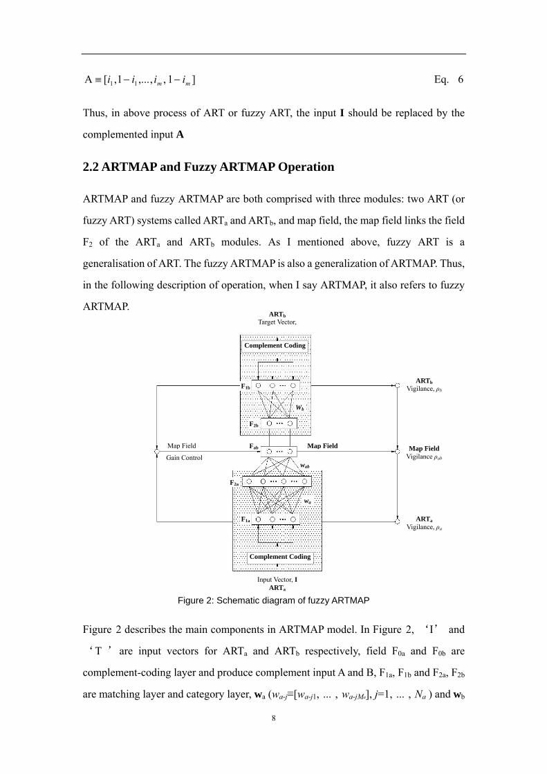
An ARTMAP (or fuzzy ARTMAP) consists of three modules, two ART (or fuzzy ART)

systems called ARTa and ARTb, and a related structure called the map field. The

ARTMAP (or fuzzy ARTMAP) can be divided into two phase: the learning phase and

the prediction phase. During the learning phase, input patterns are presented to ARTa

and their associated teaching patterns are presented to ARTb. Association between

5

ARTa and ARTb are then built at the map field. During the prediction phase, input

patterns are presented to ARTa and then recall a previously learned association with

ARTb via the map field.

Section 2.1 & 2.2 give a further description if the operation of unsupervised ART and

fuzzy ART network and supervised ARTMAP and fuzzy ARTMAP respectively.

2.1 ART and Fuzzy ART Operation

In the ART operation, it selects the first input as the exemplar or Long-Term Memory

（ ）LTM for the first cluster. The next input is compared to the first cluster exemplar.

It is classified as first cluster if the distance to the first cluster exemplar is less than a

threshold and then the first exemplar will be upgraded with the input. Otherwise, it is

the exemplar for a new cluster. This process is repeated for all following inputs. The

number of cluster thus increases with times and depends on threshold.

The major components of ART model are described in Figure 1. These components can

be grouped into two subsystems: the attentional and orienting subsystems. The field F1

and F2 are matching layer and category layer in the attentional subsystem. Each node in

F1 is connected to F2 through a set of bottom-up weights and each nodes in F2 is

connected to nodes in F1 through a set a top-down weights. In addition, the nodes in F2

are also completely connected to each other. It should be noted that the nodes in fields

F1 and F2 are used to encode patterns of Short-Term Memory (STM) activity while the

weights between nodes in F1 and F2 are used to store clusters exemplars or LTM. The

orienting subsystem receives input from the input and field F1, it will generate a reset

signal to F2 whenever the input pattern is not matched closely enough to the pattern of

STM activity across field F1.

When a input vector, I, is presented, a choice function (Eq. 1) is used to measure the

response of each node in field F2

Njw

wT

j

jj ,...,1=

+

∩Ι=β

Eq. 1

6

Figure 1: Schematic diagram of ART structure

Where β is a choice parameter of ART, wj is a vector of the top-down weigh of the j-th

cluster (wj ≡ [wj1, ... , wjM], j=1, ..., N), M is the number of node in field F1 and N is the

number of nodes in field F2, i.e. the total number of categories, the operator ‘∩ ’ is

logical ‘AND’ and the operator ‘| |’ is defined by |x| ∑≡i

ix , the L1 norm. Thus the

activity node should be chosen as the winning node J (winner-take-all), where:

},...,1:max{ ajJ NjTT == Eq. 2

The active node J will take a feedback test which is known as vigilance test in ART by

Eq. 3:

aJw

ρ≥Ι

∩Ι Eq. 3

where ]1,0[∈aρ , called the ART vigilance parameter, is an important threshold.

If the vigilance test is satisfied, resonance is said to occur and fast learning takes place

as Eq. 4:

)()()( )1()( oldJ

oldJ

newJ www λλ −+∩Ι= Eq. 4

where ]1,0[∈λ , is the ART learning rate parameter. A new node in field F2 is said to be

uncommitted node, at this case, the learning will become

Input Vector, I

F1

F2

ρ

Reset

Category Gain Control

7

Ι=Jw Eq. 5

an uncommitted node won’t become a committed until a learning happens. When

1=λ in Eq. 4 for all time, the learning is said to be fast learning.

However, if the test failed, node J is inhibited and Input I is re-transmitted to field F2 to

search a new winner node to take vigilance test again. If no node passes the vigilance

test, a new node in field F2 will be generated and the LTM weight (exemplar) of this

node will be the input I.

The choice of the ART vigilance parameter should be very careful. According to the

Eq.3, when 0=aρ , Ι

∩Ι Jw will be no less than 0, which means every new input will

be classed to the same cluster and when 1≥aρ , Ι

∩Ι Jw will be no greater than 1,

which means every new input will generate a new cluster. In this mean, the value of aρ

controls the size of the self-organised category clusters or the number of nodes in field

F2, i.e. the structure of the ART model.

Fuzzy ART incorporates computation from fuzzy set theory into ART and thus can

learn to classify both analogue and binary input patterns. By replacing the logical

‘AND’ operation ‘∩ ’ (intersection) with fuzzy ‘AND’ operation ‘∧ ’ (minimum) [19],

we can realise the fuzzy ART operation following above process of ART. Fuzzy ART is

a generalisation of ART because the minimum operation will reduce to intersection

operation in binary case.

In ART or fuzzy ART, all input vector have to be pre-processed to have equal norm in

order to avoid the category proliferation problem [5]. A F0 layer is added to the network

to accomplish the pre-processing step. Complement coding is one method to achieve

the constraint of the equal norm, where an m-dimensional

vector, },...,1],1,0[{, mji j =∈Ι is complemented to a 2m-demensionsl vector [6] as:

8

]1,,,...1,[ 11 mm iiii −−≡Α Eq. 6

Thus, in above process of ART or fuzzy ART, the input I should be replaced by the

complemented input A

2.2 ARTMAP and Fuzzy ARTMAP Operation

ARTMAP and fuzzy ARTMAP are both comprised with three modules: two ART (or

fuzzy ART) systems called ARTa and ARTb, and map field, the map field links the field

F2 of the ARTa and ARTb modules. As I mentioned above, fuzzy ART is a

generalisation of ART. The fuzzy ARTMAP is also a generalization of ARTMAP. Thus,

in the following description of operation, when I say ARTMAP, it also refers to fuzzy

ARTMAP.

Figure 2: Schematic diagram of fuzzy ARTMAP

Figure 2 describes the main components in ARTMAP model. In Figure 2, ‘I’ and

‘T ’are input vectors for ARTa and ARTb respectively, field F0a and F0b are

complement-coding layer and produce complement input A and B, F1a, F1b and F2a, F2b

are matching layer and category layer, wa (wa-j≡[wa-j1, ... , wa-jMa], j=1, ... , Na ) and wb

ARTa Vigilance, ρa

Input Vector, IARTa

ARTb Target Vector,

ARTb Vigilance, ρb

Map Field Vigilance ρab

Complement Coding

F1a

wa

Map Field

Gain Control

Complement Coding

F2a

Fab

F2b

F1b

Map Field

wab

Wb

9

(wb-j≡[wb-j1,...,wb-jMb], j=1,...,Nb) are weights vector connecting the nodes in F1a and F2a

and in F1b and F2b and wb-j≡[wb-j1,...,wb-jMb], j=1,...,Nb , Ma, Na, Mb and Nb are the number

of nodes in field F1a, F2a F1b and F2b. In the map field wab is the weight vector connecting

F2a and Fab and the number of nodes in field Fab equals to that in F2b and the one-to-one

link between each corresponding pair of nodes is permanent. An ARTMAP operation

will be divided into two phase: supervised learning phase (or training phase) and

prediction phase (or testing phase).

2.2.1 Supervised learning

When a input vector and the related target vector are presented, the both vector will be

complemented in field F0a and F0b, then the both ART modules will take

self-origanisation as the process described in section 2.1. Note that at the phase, the

weight upgrade will not take place and the weight vector wj will be replaced by waj and

wbj and the input vector I will be replaced by the complemented input vector A and B in

ARTa and ARTb respectively. After all, after this process, a category node J (J∈1, …,

Na) in F2a and a category node K (K∈1, …, Nb) in F2b will be chosen as the winner

nodes in ARTa and ARTb. Then the map field is activated.

In the map field, nodes in field F2a and Fab have a permanent link, i.e. category node P in

F2a will only associate to a special node Q in Fab, and thus we have:

⎩⎨⎧

≠=

=− QkQk

w Pkab 01

Eq. 7

Once winner node J is chosen in ARTa, map field will give a prediction node k in Fab, i.e.

wab-Jk = 1. Because nodes in Fab and F2b have relationship of one-to-one connection, the

prediction will compare to the chosen node in field F2b. If k = K, the process will be

finished and weight vector wa-J will be upgraded by Eq. 4. If k ≠ K, a process called

match-tracking will be launched

At the beginning of each input vector presented, the vigilance parameter of ARTa,

vigilance parameter, aρ is the pre-defined value aρ . Whenever a winner node J in

10

field F2a make a incorrect prediction, aρ will be increased to

δρ +Α∧Α

= −Jaa

w Eq. 8

where δ is a positive value just a little larger than zero. Thus the vigilance test in Eq. 3,

will fail and node J in field F2a will be inhibited for the new winner searching in ARTa.

The process will repeat until a winner node J which can give a correct prediction or no

such node exists in field F2a. If node J can give a right prediction, the weight vector will

also have to upgrade by Eq. 4 to finish the learning. If there is no such node, an

uncommitted node J will be added in F2a. In ARTa, the uncommitted weight vector wa-J

will be upgraded by Eq. 5 and in map field, weight vector wab-J will be updated

according to Eq. 7.

If node K in F2b, is a new category, i.e. an added uncommitted node in ARTb, Fab will

also add a corresponding node, and the winner node J in field F2a will be associated to

this node. Weight vector wab-J will be updated by Eq. 7. Weight wa-J will also be

upgraded by Eq. 4, or if node J in ARTa is also an uncommitted node, it will be

upgraded by Eq. 5 just like the updating of weight vector wb-J.

2.2.2 Prediction Phase

In the prediction phase, things become much simple. When a input pattern is presented

to ARTa, a winner node J will be chosen in F2a, then map field will gives a prediction K

in Fab and because the one-to-one link between field Fab and F2b, node K will be chosen

in field F2b, node K will response a exemplar, i.e. the weight vector connects node K to

field F1b, then the weight vector wb-J will be the prediction targets vector. Normally in

any problem domain, the so called meaningful category will be very simple, therefore,

the target vectors which can be the input of ARTb are always simple and binary, then the

exemplar or the weight, wab, connecting field F1b and F2b also should be binary. Thus,

the given prediction target vector will be a meaningful category in the problem domain.

11

2.3 Simplified ARTMAP

Because the meaningful category in problem domain always be very simple, the ARTb

module in ARTMAP may be a computation burden. In practice, we always employ a

simple scheme called simplified ARTMAP. Figure 3 gives the structure of simplified

ARTMAP.

Figure 3: Simplified fuzzy ARTMAP

In simplified ARTMAP, module ARTb is replaced by a pattern class vector which

represents the known classes in the problem domain. In the map field, nodes in Fab also

have the same number of node with the size of pattern class vector, i.e. the number of

the known classes. Thus this map field becomes more like to a ‘look-up table’ [15].

Also to reduce the computation, in simplified ARTMAP, the category choice parameter,

β, is set to a positive value just a little larger than zero and the learning rate, λ, is set to

be 1, which is the so called fast learning. Thus in simplified ARTMAP, the only

changeable parameter is the vigilance of ARTa, ρa.

2.4 Advantages and Limitations

ART and ARTMAP family are developed to overcome the stability-plasticity dilemma.

These models based neural networks offer a number of advantages over other forms

Input Vector, IARTa

Map Field Vigilance ρab

ARTa Vigilance, ρa

Complement Coding

F1a

wa

Map Field

Gain Control

ARTb Target Input,

Pattern Class

Map Field

F2a

Fab

wab

12

of neural network. First, the learning does not require any stop, thus an ART or

ARTMAP is suitable to be trained online. Another property of ART family related to

the online learning is that the learning is very fast and thus they are also suitable to

utilise a real time online learning. Second, ART and ARTMAP models can perform

robustly under noisy conditions in a non-stationary environment. It is true that ART

and ARTMAP models do not need a well bounded and stable input environment, this

allows them to be utilized in a much wider variety of application. And finally, an ART

or ARTMAP model has only one parameter to be tuned and the original structure of

the model is just determined by the dimension of the input vector and target vector.

Thus the system validation will take much less time than the other type of neural

networks such as MLP or RBFNN.

The primary disadvantage of ART and ARTMAP models is the lack of a Bayesian

interpretation. There is also not a threshold of decision making. Although vigilance

parameter can be regarded as a threshold, it affects more on the structure of the ART

model. This two limitations result the lack of further investigation.

13

Chapter 3: Study Design

3.1 Data Analysis and Pre-treatment

This study is based on the clinical and electrocardiogram (ECG) data of 3642 patients

which were collected in the Emergency Department of four different hospitals [12]. In

the Royal Infirmary of Edinburgh, 1253 samples were collected over four months

(August to December, 1995), the collected data in Western General Hospital,

Edinburgh are 1268 samples over six months (February to August, 1996), the number

of samples in the third hospital, Northern General Hospital, Sheffield, is 626 and the

time of collecting is from September to December, 1992, and there are only a small

sample of patients collected from Leicester Royal Infirmary, the number is 152. All of

these cases have the main symptom o f non-traumatic chest pain.

All of those patients are diagnosed to ACS, SCP and NCP. In the three-class problem,

class 1 represents ACS, class 2 represents SCP and class 3 represents NCP and there

are 1603 (44%) ACS, 888 (24.4%) SCP and 1151 (31.6%) NCP patients. And in the

two-class problem, the patients are classified to ACS and non-ACS where in the

system, class 0 represent non-ACS and class 1 represent ACS. In fact, non-ACS is the

sum of SCP and NCP. Thus we have 2039 (about 56%) cases of non-ACS. The

inappropriate diagnoses of these data is very low (about 2%) [12].

For each sample of patient, 40 features are collected. Most of these features are

collected as binary data expect the features ‘age’ and ‘worsening’ which present how

many hours the chest pain lasted are continuous data.. For Fuzzy ART operation, the

continuous value should be transferred to fuzzy set according Zadeh’s theorem [20].

For the feature ‘age’, two classes of membership are chosen and the shape of the

membership function is logistic sigmoid and its complement. Thus, for the feature

‘age’, the membership function assign value µA(u) and µB(u) to each u as:

14

8)50(

8)50(

1

11)(

1

1)(

uB

uA

eu

eu

−

−

+−=

+=

µ

µ

Eq. 9

the parameter 50 is chosen as the Crossover Point, which means that at age 50, µA(u)

= µB(u) = 0.5 and the division parameter 8 is selected to control the shape of logistic

sigmoid near the point 50 which is the sensitive age of ACS. Figure 4 is the diagram

of membership functions for feature ‘age’.

Figure 4: Fuzzyfication function membership function of ‘age’

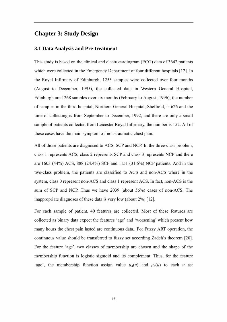
For feature ‘worsening’, we choose five classes of memberships and the related

membership functions are:

⎪⎩

⎪⎨

⎧≤<−−≤<−

=

⎪⎩

⎪⎨

⎧≤<−−≤≤

=

⎩⎨⎧ <=<=−

=

otherwiseuuuu

u

otherwiseuu

uuu

otherwiseuu

u

C

B

A

0241212/)24(1241212/)12(

)(

0241212/)12(1

12012/)(

012012/1

)(

µ

µ

µ

µB(u) µA(u)

15

⎪⎩

⎪⎨

⎧>≤<−

=

⎪⎩

⎪⎨

⎧≤<−−≤<−

=

otherwiseu

uuu

otherwiseuuuu

u

E

D

0481

483612/)36()(

0483612/)36(1362412/)24(

)(

µ

µ

Eq. 10

Figure 5 is the diagram of membership function for feature ‘worsening’

Figure 5: Fuzzyfication function membership function of ‘worsening’

To avoid the category proliferation problem, complement coding is needed for each

feature to ensure that the input vectors have equal norm. However, for fuzzy set

vectors, it always have same norm of 1, we do not need complement codes for those

fuzzy set vectors. Those binary should be complemented by the Eq. 6 and then

combined with the two fuzzy set vectors to be the input of the fuzzy ARTMAP

operation.

3.2 M-fold Cross Validation

Cross-validation (CV) is the simplest and most widely used method of estimating

generalisation error based on the idea of re-sampling. The resulting estimates of

generalisation error are often used for choosing among various models, such as

µB(u) µA(u) µC(u) µD(u) µE(u)

16

different structures, or for setting a good value of regularization parameter for a fixed

structure. In the simplified fuzzy ARTMAP, the structure of the network is determined

by the data set and the order of the data sets, however, it is still helpful in choosing the

vigilance parameter for a particular set of data.

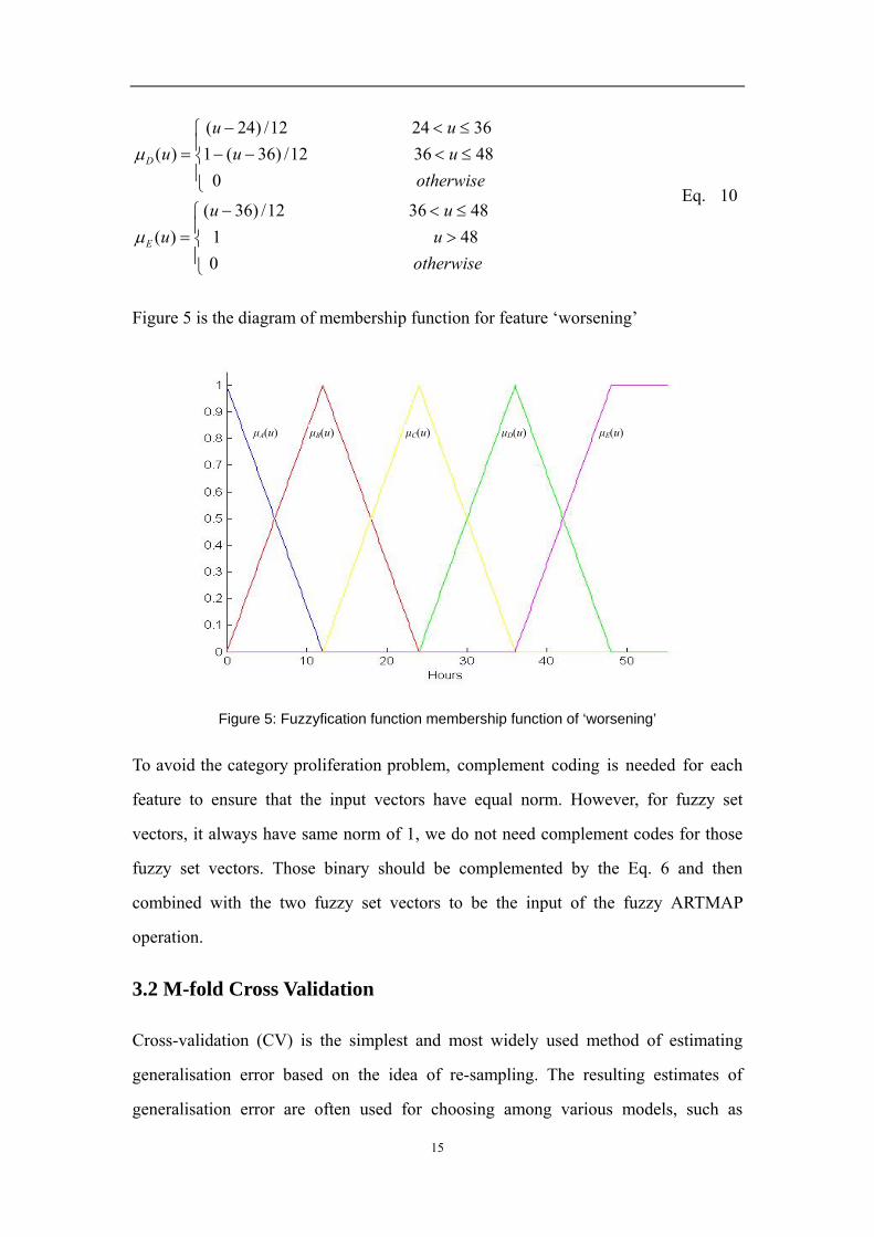
In M-fold cross validation, the data sets are divided into M subsets of (approximately)

equal size and the neural network is trained M times. Each time, one of the subsets is

leaving out from training but using it for test and compute any performance criterion

interests us, for example, mean square error, accuracy rate, etc. Figure 6 illustrate the

way the data are treated in five-fold cross validation. Here, we are at the third and

forth step of the procedure. Note that training is done using all but one of the subset,

Xi.

Figure 6: Five –fold Cross Validation Procedure at 3rd & 4th Step

In this dissertation, we don’t know what a good value for the vigilance parameter is,

so we conduct M-fold CV for a range of value of ρ. The value of ρ resulting in the

best CV performance is then chosen. Evidently this is not truly optimal but it will be

the best of the value tested.

Train

Train Train

Train

Train

Train

Test

Train

Test

Train

3rd Step 4th Step

Fold 1

Fold 2

Fold 3

Fold 4

Fold 5

17

3.3 On-line Learning Method

First, Let us recall a doctor’s growing experiences. Going to be a professional doctor,

there are two main periods which have to be taken. The first step is to be a student of

medical department in a university. During this period, the professional medical

theorem and shills will be given in the first three or four years. This is a significant

part which could provide the basic theory and knowledge for the students’ further

study and practice. At the last one or two years, the students will study in the hospitals

where provide them the chances to face the real patients as well as practice of the

medical theory. In the hospital, the students will get their initial experience which

means that they could be able to diagnose for some simple cases or the cases which

have some obvious features. At the same time, these cases will surly strengthen their

experiences as well. The second period is a kind of study over through a doctor’s

whole career life. The career life is a process to enrich a special database which could

provide some critical point of diagnose for the doctor by classified the patient cases.

The positive classification generalised from the doctor’s further study which include

participating the consultation or learning from the experienced doctors.

Our on-line learning method could simulate this process because the fuzzy ARTMAP

operation can overcome the stability-plasticity dilemma which means, in our problem

domain, when the neural work ‘learns’ a new case, the previous cases will not be

‘forgotten’. Thus we can sketch our on-line learning strategy: First, the structure of

the neural network should be determined, for simplified ARTMAP, we have to decide

the dimensions of the input vector, the number of classes in the problem domain and

the vigilance parameter of the neural network. This structure represents a person who

want to be a doctor and of course this ‘person’ has no any knowledge of medical

diagnosis because there is no category in field F2a, no connecting weight between

field F1a and F2b and no map field weight. And then, the neural network will be trained

by a certain number of samples (we called a hot start) which can form a certain

number of categories and its weights vectors connected to field F1a (LTM) and related

weights vectors in map field. This learning stage is equal to the person’s studying in

18

his university. In this phase of learning, the more clusters are formed in field F2a, the

more feature the neural network have learned and the better performance will be get

in the prediction/on-line learning phase. In this online learning system, 900 ACS cases,

450 SCP cases and 650 NCP cases which are in a random order are chosen to train the

neural networks. Table 1 gives the number of samples of each class for the total data

and hot start train sets and their portion. At last, it is the prediction and on-line

learning phase. This phase equals to the whole life learning of a doctor. It should be

noted that wrong classification learning is very dangerous in an ARTMAP network

because any learning in an ARTMAP operation will form a long term memory which

include the self-organised category and related weight vectors connected to field F1a

and map field node. When a same case or a case which can be self-organised to the

same category is presented in the prediction phase, the LTM will leads to a wrong

prediction. Therefore, in the on-line learning phase, the true value of class will be

presented instead of the prediction of class. In fact, this is more close to the things in

real world. In the whole life learning of a doctor, he maybe makes some wrong

diagnoses, however, these wrong diagnoses should be corrected either by himself or

other doctors. Thus, the doctor will always remember the right information but forget

the wrong diagnoses. However, an ARTMAP operation can not ‘forget’ these wrong

LTM. Modified fuzzy ARTMAP [13, 14] seems to be able to ‘forget’ some LTM by

ignoring some LTM which are presented with lower frequency, but this is not the

point we discuss in this paper.

Table 1: Classification of Chest Pain Suffers

Non-ACS Final Diagnosis ACS SCP NCP Total Number 1603 888 1151 3642 Whole

set Proportion 44% 24.4% 31.6% 1 Number 900 450 650 2000 Train

set Proportion 45% 22.5% 32.5% 1

3.4 Voting Strategy

The concept of voting strategy is original from the old saying ‘two head is better than

19

one’. Normally, voting strategy is using for off line prediction because the operating

of several neural networks will take more time which may not meet dead line of the

on-line operation. However, for a clinical support system, the so called ‘on-line

learning’ is not a time critical task. I do not mean that the time is not important in this

clinic support system, but in fact, in our voting operating, a single prediction will just

take no more than one second which is much shorter than the time for a doctor or an

operator to input the feature data of a patient. For the same reason, our online learning

employs the multi-epoch to optimise the categories and weight vectors in F2a

The formation of category cluster in ARTMAP operation is affected by the order of

presentation of input data items [6]. Thus, the same data presenting to an ARTMAP

with different order will result different categorisation of the train data thus different

performance in the future prediction of test data. This effect is particularly marked

with small train samples and /or high-dimensional input vectors where the train

samples may not fully representative of the problem domain [9]. And also, as we

know in an ARTMAP operation, a most important parameter, vigilance parameter of

ARTa, affects the category cluster of nodes in field F2a and thus affects the future

prediction of test data. Both of these characters of ARTMAP operation give us the

resources to build up our different heads (voters) for the voting strategy as below.

First, three fuzzy ARTMAP neural networks with different ARTa vigilance parameters

from 0.1 to 0.3 are formed. Then the three neural networks will be trained by the train

samples with six different arbitrary random orders and 18 different

‘heads’---ARTMAP neural networks are built up. In the prediction and on-line

learning phase, when an input vector is presented, each individual network gives its

prediction in normal way. The number of each category (include the result that is

unable to give a prediction) is then accounted and the one with the highest number (or

the most ‘votes’) is the final prediction result. The higher ratio of the max votes to the

total number of neural network will gives a more confidence of the prediction. At last,

each neural network will be updated by the presented input and the true value of

classification.

20

Chapter 4: Result and Analysis

In this chapter, the performance of the on-line learning strategy will be demonstrated.

Here two important definitions will be given first:

Accuracy (ACC): Denotes as ratio of the number of the correct prediction over

the number of total prediction.

Specificity (SPEC): This is a conception just for two class problem. It denotes as

the ratio of the number of correct negative prediction (non-ASC) over the total

number of the true negative prediction.

Sensitivity (SENS): For two-class problem, it is the ratio of the number of correct

positive prediction (ACS) over the total number of the true positive classification.

For three-class problem, the sensitivity for a particular class is defined as the ratio

of the number of correct prediction of the class over the total number of the true

value of the class. For example, the sensitivity of class 1 (SENS1) is the ratio of

the number of correct prediction of class 1 over the total number of the samples

of class1. Thus, SENS1 represents the sensitivity for ACS, SENS2 represents the

sensitivity for SCP and SENS3 represents the sensitivity for NCP.

Accuracy, specificity and sensitivity are the main reference to evaluate the

performance of the decision system. However, as a clinic support system, a doctor

may care more about the parameter of sensitivity or specificity, especial for the

sensitivity for ACS in this decision system because ACS is the main challenge in the

emergency medicine. In this chapter, the result of system validation will be carried out

firstly, the purpose of the system validation is to choose the best voters for the voting

strategy. Then, the performance online learning systems will be demonstrated: first, a

three-class system with a single fuzzy ARTMAP network with no hot start

demonstrates the potential of a fuzzy ARTMAP to diagnosis ACS. And then a detail

analysis of the performance of a three-class system employed voting strategy

21

(18voters) with a hot start of 2000 samples is carried out. And finally there will be a

comparison of between the performances of the two class system and three class

system with the voting online strategy. To eliminate the effect of the order of the data

sets, ten run of different order of data sets are taken and the performance evaluation

will be based on the average of the result of the ten run. Thus the average of the

accuracy, specificity and sensitivity over the ten run will be plotted as well as their

standard deviations at some points.

4.1 System Validation

As I mentioned in section 2.3, a simplified fuzzy ARTMAP just have one changeable

parameter, vigilance parameter. The structure of the model depends on the

autonomous operation on the data set and the order of the set. Thus, this system

validation is in fact to determine suitable vigilance parameters. In this section, we will

give the best vigilance parameters for simplified fuzzy ARTMAP model for the data

set in the three-class problem.

Here, we use a five-fold CV for choosing the vigilance parameters. Ten multi-run with

different random of data set are also used. The performances (accuracy and sensitivity)

are recorded for each run and the average of the performances and their standard

deviation are also calculated. Table 2 gives the result. It should be noted that the

performance for each run is the statistic of the total five-fold test.

As we can in Table 2, vigilance parameters 0.1, 0.2 0.3 and 0.4 give better result on

performance. In this paper, I choose 0.1, 0.2 and 0.3 as the vigilance parameters of the

voters for the voting strategy. Obviously, these are not the optimal result, but they are

the best within our test parameters. The result is also true to the two-class problem.

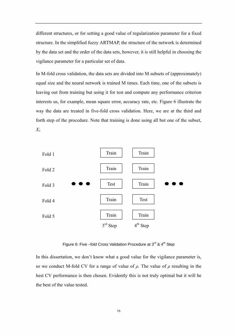
4.2 Online Learning without Hot Start with Single Fuzzy ARTMAP

Here the single fuzzy ARTMAP network is chosen as vigilance parameter ρa = 0.1

which has a best performance in the system validation (see Table 2). Figure 7 shows

the performance of this online learning system.

22

Table 2 : Five-fold cross validation for different vigilance parameters

Vagilince Run1 Run2 Run3 Run4 Run5 Run6 Run7 Run8 Run9 Run10 Ave SD

ACS(%) 68.7 67.6 68.5 68.4 68.1 68.1 68.0 68.3 68.8 67.7 68.2 0.4

SENS1(%) 76.9 72.9 75.6 75.3 75.0 75.5 75.9 76.0 75.2 76.5 75.5 1.0

SENS2(%) 51.0 52.7 51.7 51.7 52.0 50.3 50.2 51.1 53.5 48.9 51.3 1.30.1

SENS3(%) 70.9 71.6 71.5 71.5 70.9 71.4 70.7 70.9 71.5 69.7 71.0 0.5

ACS(%) 68.9 67.4 67.4 68.0 67.0 68.1 67.4 66.9 67.4 69.8 67.9 0.9

SENS1(%) 74.3 75.3 74.9 75.3 75.0 76.4 74.4 74.9 74.3 76.2 75.1 0.7

SENS2(%) 55.4 49.1 51.8 49.4 50.3 51.4 49.9 49.5 50.5 53.0 51.0 1.90.2

SENS3(%) 71.6 70.6 69.0 72.3 68.8 69.4 71.2 69.2 70.8 73.7 70.7 1.5

ACS(%) 67.4 67.6 68.9 67.7 68.6 68.3 68.8 67.4 67.9 69.1 68.2 0.6

SENS1(%) 73.1 73.9 76.0 75.7 74.9 76.3 74.8 75.0 75.5 76.0 75.1 0.9

SENS2(%) 49.8 50.1 51.9 50.2 52.7 51.2 52.5 51.3 51.8 54.0 51.5 1.20.3

SENS3(%) 72.9 72.2 71.9 70.0 72.0 70.2 73.1 69.3 69.6 71.2 71.2 1.3

ACS(%) 67.9 68.2 67.7 67.2 68.0 67.1 69.2 68.9 66.8 69.4 68.0 0.9

SENS1(%) 73.8 74.0 72.6 73.8 73.4 74.1 77.1 74.6 72.4 75.0 74.1 1.3

SENS2(%) 52.0 54.2 55.0 49.5 54.5 50.6 50.2 53.7 53.0 54.2 52.7 1.90.4

SENS3(%) 72.0 70.9 70.5 71.6 70.8 70.0 72.9 72.4 69.5 73.3 71.4 1.2

ACS(%) 65.7 66.6 65.7 67.4 66.2 66.6 67.1 66.1 68.1 65.7 66.5 0.8

SENS1(%) 69.1 70.1 69.3 71.5 68.9 72.0 71.2 69.5 72.5 69.6 70.4 1.2

SENS2(%) 52.7 52.3 52.0 52.9 54.1 50.6 54.5 54.1 56.4 53.0 53.3 1.50.5

SENS3(%) 70.8 72.5 71.2 72.7 71.6 71.2 71.1 70.4 71.0 69.9 71.2 0.8

ACS(%) 64.0 63.3 61.9 62.0 62.5 61.8 64.8 63.7 64.1 62.9 63.1 1.0

SENS1(%) 65.1 62.3 62.6 62.0 62.9 62.4 65.0 66.0 63.8 62.9 63.5 1.3

SENS2(%) 53.7 55.7 52.5 53.2 54.8 51.5 55.2 52.3 57.7 54.3 54.1 1.80.6

SENS3(%) 70.2 70.4 68.2 68.7 67.7 68.7 71.6 69.1 69.5 69.5 69.4 1.1

ACS(%) 57.3 58.8 59.8 59.6 57.0 59.2 58.2 57.4 59.3 57.5 58.4 1.0

SENS1(%) 54.8 55.5 58.0 58.8 54.0 56.7 55.9 52.9 57.8 55.7 56.0 1.8

SENS2(%) 49.0 55.8 52.5 50.6 48.6 55.2 51.3 52.9 52.8 48.8 51.8 2.40.7

SENS3(%) 67.1 65.8 67.7 67.6 67.6 65.8 66.8 66.9 66.4 66.5 66.8 0.7

23

0 500 1000 1500 2000 2500 3000 35000.2

0.3

0.4

0.5

0.6

0.7

0.8

No. of Samples

Per

form

ance

ACCSENS1SENS2SENS3

Figure 7: Performance, non-hot-start online learning with single fuzzy ARTMAP model

Generally speaking, as increasing of the number of samples, there is a rapid

improvement of performance in the early stage of online learning and then the

tendency of increasing becomes gently or some fluctuation occurs and at last the

value of accuracy and sensitivity for ACS, SCP and NCP converge to a stable value

respectively. At the same time, there is also a gradual reduction in the spread of

performance for different runs and the performance of an individual run has a

tendency towards the average performance. This means the averaging of different

runs is not necessary when the number of samples is big enough and a truly online

learning system can be formed.

There are some feature should be noted in the early stage of online learning: Firstly,

the performance of the system increases sharply with a very small number of samples

(less than 20 samples), this shows that the fuzzy ARTMAP is a fast learning neural

network. Secondly, sometimes, fuzzy ARTMAP will fail to make a prediction,

especially in the early stage of learning and when vigilance is big enough (E.g. ρa>0.7

in this system). In the first several samples of learning, maybe every sample presented

to the neural network will form a new category in field F2a and a larger vigilance

parameter will result a more categories in field F2a as the increasing of samples. All of

these new categories can not recognize a pattern until a learning is performance. This

is also the reason of the fluctuation of performance in the early stage of learning. And

24

finally, the poor performance in the early stage affects the long-run results. However,

this effect will be eliminated with the increasing of samples.

Although this no hot start single fuzzy ARTMAP system shows some potential

characters in online learning, the poor performance is an inevitable problem.

4.3 Voting Online Learning Strategy---3-Class Problem

The details of this voting online learning strategy have been described in section 3.4.

The vigilance parameters are chosen as ρa = 0.1, 0.2 and 0.3 because of the good

performance in system validation (Table 2). And using different order of train sets is

to reduce the effect of performance with the order of the train sets. For the test and

online learning, ten different run with different random order are also taken because

the order of test sets also affect the performance of system. To evaluate the

performance of the system, two techniques are used: the first is ‘sample replacement’

in which the train sets will be put into the test sets at a random order and the second is

‘no sample replacement’ in which the train sets will not put back to the test sets,

which is a more challenge task. Figure 8 and Figure 9 show the performance of the

online system with sample replacement and no sample replacement method

respectively

0 500 1000 1500 2000 2500 3000 35000.6

0.65

0.7

0.75

0.8

0.85

0.9

0.95

1

No. of Samples

Per

form

ance

ACCSENS1SENS2SENS3

Figure 8: Performance of online voting strategy, 2000 samples’ hot start

(with sample replacement)

25

0 200 400 600 800 1000 1200 1400 16000.4

0.45

0.5

0.55

0.6

0.65

0.7

0.75

0.8

0.85

0.9

No. of Samples

Per

form

ance

ACCSENS1SENS2SENS3

Figure 9: Performance of online voting strategy, 2000 samples’ hot start

(no sample replacement)

In these two figures, we can see some same characters with the single fuzzy ARTMAP

network. First, the performance improve rapidly to a rather high degree, in fact,

because of the 2000 samples hot start, the improvement is much quicker than that no

hot start system. Second, the standard deviation of different runs reduces continuously

as the increasing of the samples and has the trend to converge to zero which suggests

that a truly online system can be used. And there are also some peaks and fluctuation

in the early stage of learning.

However, there are also some difference between the voting strategy and the single

neural network. First, of course, the total performance have a obvious improvement,

either the sample replacement or the more challenge task, no sample replacement, all

of the four items, ACS, SENS1, SENS2 and SENS3 have a final performance

improvement at least 15%, this is due to the voting strategy as well as the 2000

samples’ hot start. Another difference is no obvious continuous improvement for the

second method. Instead, after the performance promotion in the first few samples, the

performances have a tendency of decreasing with some fluctuation and then converge

to a stable value.

26

4.3.1 What the System Learned in the Online Learning

As I mentioned above, the performance of the system does not show a continuous

improvement. However, this does not mean that the system has not learned any thing.

In fact, because of the 2000 samples of hot start, the system have formed a rather

plenty of knowledge (LTM), on another word, the system is an experienced ‘doctor’

now. But as a clinical system, it much possible to meet some cases that it can not

recognise or it will make a wrong decision, our online learning is to avoid these kinds

of wrong decision. If the system make a right decision, the learning will upgrade

related weight vector in ARTa, if the system make a wrong decision, the learning will

trigger the match tracking which will result another related weight vector updated or a

new category added in field F2a and related nodes in map field and weight vectors will

also be added as well, if the system can not make a decision, the learning will also

result a new in field F2a. Figure 10 shows that the number of categories of the total 18

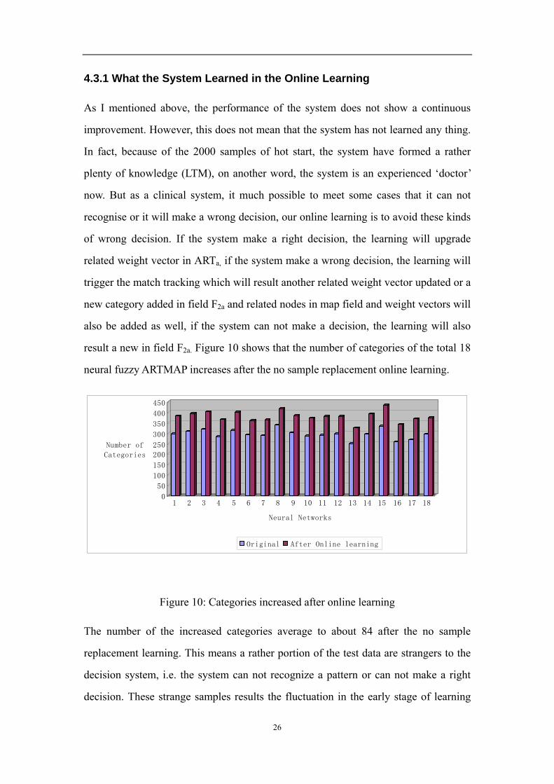
neural fuzzy ARTMAP increases after the no sample replacement online learning.

0

50

100

150

200

250

300

350

400

450

Number of

Categories

1 2 3 4 5 6 7 8 9 10 11 12 13 14 15 16 17 18

Neural Networks

Original After Online learning

Figure 10: Categories increased after online learning

The number of the increased categories average to about 84 after the no sample

replacement learning. This means a rather portion of the test data are strangers to the

decision system, i.e. the system can not recognize a pattern or can not make a right

decision. These strange samples results the fluctuation in the early stage of learning

27

and as the increasing of the number of the samples, the performance will trend to be

stable. In fact this process is just like the decision process of a human being. In the

early stage of a medical school graduated student working in a hospital or a clinical,

his performance will be fluctuated. Some of them will get a rather high performance

within a several weeks, this depends on the knowledge he mastered. This knowledge

equals to the hot start of the systems. If he has no related knowledge, i.e. the system

has no hot start, he will also have a graduate improvement in the performance, but this

progress will be much slower than those who have enough knowledge. Then as the

time going on, he will meet more difficult cases of patients, his performance will have

some fluctuation, but at the same time, the more experiences or knowledge are built

up. And finally, as more experiences and knowledge built up, he will get a stable

performance upon his career. Another point is his performance in his career depends

on what he learned in his medical school in some extent, normally, a good student will

have a good performance in his career although this is not absolute in our true life.

The following three figures give the performance of the online strategy with different

samples of hot start. In these Figures, Figure 11 has no hot start and we can not form

the voters with different order of the train set. In the case, 15 fuzzy ARTMAP models

are built with different vigilance from 0.05 to 0.75. Figure 12 has a hot start with 200

samples and Figure 13 has a hot start with 1000 samples. Compare these three figures

and Figure, we can find the performance improvement as the increasing samples of

hot start.

0 500 1000 1500 2000 2500 3000 35000.2

0.3

0.4

0.5

0.6

0.7

0.8

No. of Samples

Per

form

ance

ACCSENS1SENS2SENS3

Figure 11

28

0 500 1000 1500 2000 2500 30000.4

0.45

0.5

0.55

0.6

0.65

0.7

0.75

0.8

0.85

0.9

No. of Sample

Per

form

ance

ACCSENS1SENS2SENS3

Figure 12: Performance of online voting strategy, 200 samples’ hot start

(no sample replacement)

0 500 1000 1500 2000 25000.4

0.45

0.5

0.55

0.6

0.65

0.7

0.75

0.8

0.85

0.9

No. of Samples

Per

form

ance

ACCSENS1SENS2SENS3

Figure 13: Performance of online voting strategy, 1000 samples’ hot start

(no sample replacement)

4.3.2 Sample Replacement and No Sample Replacement

Comparing Figure 8 and Figure 9, we can see sample replacement yields a much

better performance than no sample replacement, however, we can also find a slightly

continuous decreasing of the performance of the sample replacement. This is because

of the small sample size. In fact, when I test the hot start system with train sets, it

always gives a 100% accuracy prediction. It is also true for a single fuzzy ARTMAP

network. This difference may be eliminated when the number of samples is big

enough

29

Normally, when we get a 100% accuracy prediction on train sets, it will be said to be

over trained, or the system is not generalised. But in this case, it is not. For the

simplified fuzzy ARTMAP, the only changeable parameter is the vigilance parameter.

I try to change the vigilance parameter, ρa, from 0 to 0.7 (when ρa > 0.7, the train will

take a much long time because of the category proliferation and for the fuzzy

ARTMAP, over train is brought from a larger vigilance), I get the same result. I think

this is because of the under sampling, after all it is an 83-dimension input vector, and

in the problem domain, it has 40 features. Even if all these 40 features are binary

value, it has 240 possibilities. Thus, we can explain this in two-dimension as in figure

14:

Figure 14: Categories without intersection

In this figure, we have three self-organised categories C1, C2 and C3 which are

assigned to class 1, class 2 and class 3. Now a new data x is presented and class 1

wins the competition and pass the vigilance test (we assume the vigilance is a lower

value), however, data x is belong to class 2, then match tracking is triggered and result

a new category C4, or category C2 expand to C’2, because of the under sampling, there

is no intersection part between C1 and C’2 or C4 or there is no sample in the

intersection part. Then after a multi-epoch train, the categories and weight vectors are

optimised and these train data can be classified correctly by the system.

C1

C2

C3

C4

C’2

x

30

4.3.3 Poor Performance on Classifying SCP and NCP

In all of the above performance figures, we can also note that the performance on

classifying SCP and NCP is much poorer than that on ACS. This is because the

character of ACS is more obvious but the character of SCP is not so clearly separated

to NCP, this is also shown by the countingring table (Table 3)

Table 3 is the countingring table for total statistics of the no sample replacement

prediction and online learning. As we can see in the table, 196 (about 32.7%) cases of

NCP are predicted to SCP and 76 (about 17.5%) of SCP are predicted to NCP, this

means that many features of NCP and SCP are very close. These close features result

Table 3: Countingring table for no sample replacement

Predicted Value

ACS SCP NCP

ACS 598 90 15

SCP 68 294 76

True

Value

NCP 27 196 376

the difficulty on classifying this two classes and thus affect the performance of the

system. This also can be proofed by a two-class model. Normally, a two-class

decision is much easier than a three-class problem. In this model, I also use the voting

online learning with hot start. There are total 2039 samples which belong to SCP and

NCP. 450 samples of SCP and 65osamples of NCP are chosen as hot start train sets,

these number are the same as our three-class problem. Again 18 fuzzy ARTMAP

networks are trained with vigilance parameter 0.1, 0.2 and 0.3 and six different

random order. Then the no sample replacement learning is performed. Figure 15 is the

average performance of ten run and Table 4 is the countingring table for the total

statistics.

31

0 200 400 600 8000.4

0.45

0.5

0.55

0.6

0.65

0.7

0.75

0.8

0.85

0.9

No. of Samples

Per

form

ance

ACCSENS2SENS3

Figure 15: Performance of classification of SCP & NCP with online strategy

(450 SCP and 650 NCP hot start, no sample replacement)

Table 4: Countingring table for the SCP vs. NCP problem

Predicted Value

SCP NCP

SCP 342 96 True

Value NCP 229 386

Performance shown in Figure 15 get some improvement in accuracy, however, these

improvements are based on the reduction of class ACS. But the reduction of class

ACS can not eliminate the close features of SCP and NCP. From Table 4 we can see,

229 (about 37.2.0%) of NCP samples are predicted to SCP and 88 (about 21.9%) of

SCP are predicted to NCP. However, these close features are still separable. When I

train the system with whole set of samples and then test on these samples, the 100%

accuracy of prediction is also achieved. As I mentioned above, this is not over train, it

is due to the sampling data are separable.

4.4 Two-class Vs. Three-class

In this section, the performance of the online strategy regard to the two-class problem

is commented. According the Table 1, the train sets include 900 ACS samples and

1100 non-ACS samples. Again, 18 voters are trained with three different vigilance

parameters, 0.1, 0.2 and 0.3 and with 6 different random orders of the train sets.

Figure 16 shows the average performance over ten different runs with different order

32

of the test sets. It should be noted that this figure of performance is outcomes from the

no sample replacement method.

0 200 400 600 800 1000 1200 1400 16000.6

0.65

0.7

0.75

0.8

0.85

0.9

No. of Samples

Per

form

ance

ACCSENSSPEC

Figure 16: Performance of two-class problem with online learning strategy

(900 ACS and 1100 non-ACS hot start, no sample replacement)

The general tendency of the curves is just like those in the three-class problem which

have been analysed clearly in section 4.2. Here the comparison of figure and figure

which both use the no sample replacement method will be implemented. As a two

class problem under the same condition, of course, the performance improved. The

final accuracy rate increased from about 77.1% to 87.3%. This also means in the data

space, the character of ACS or non-ACS is more obvious. However, if we compare

SENS in Figure 16 and SENS1 in Figure 9 which both represent the sensitivity of

ACS, we can find in the two-class system, the sensitivity of ACS decreases from

about 85.1% to about 80%. We can also see this in the following countingring table

Table 5: Countingring table for the two-class problem

Predicted Value

ACS non-ACS

ACS 567 136 True

Value non-ACS 65 874

In Table, we can see that 136 ACS cases (about 20%) are predicted to be non-ACS

33

and in the three class problem totally 105 ACS cases (about 15%) are predicted to be

non-ACS. However, we can consider another problem, accuracy of ACS prediction, in

the two-class problem the accuracy rate of ACS prediction is about 89.7% and the

data in three-class problem is 86.3%. This means either in two-class system or in

three-class system, the prediction is highly reliable. On the other hand, we consider

the error rate of non-ACS prediction, the data in the two-class system is about 13.5%

while in three-class problem is about 10%, this means those cases which are predicted

to be non-ACS should still be highly consider.

34

Chapter 5: Conclusion

This fuzzy ARTMAP model based online learning strategy has demonstrated its high

performance in diagnosis acute coronary syndromes and has the following advantages:

The first is associated to the advantage of fuzzy ARTMAP models, the capability of

robust performing under noisy conditions in non-stationary environment is specially

suit for the medicine diagnosis problem because of the randomicity of the patients, the

properties of autonomous operation which overcoming the stability-plasticity

dilemma makes it possible to perfect the system continuously within the whole life of

the system operating. Second, the voting strategy with high performance voters can

make sure the high performance of the system, and further more, these high

performed voters can be improved during the online learning. And finally, hot start

strategy can not only give a good performance in the early stage of online learning but

also determine the final performance of the system.

However, the system still needs the following improvement: the first we concern is

the performance of classifying the stable cardiac pain and non-stable cardiac pain.

Because of the high similarity in feature of these two classes, more samples of the two

classes are required to create high separated categories in field of F2a to improve the

performance of classify these two class. Second, because of the autonomous operation

of fuzzy ARTMAP models, the category proliferation is inevitable and category

pruning [9] should be employed.

Another point we should be noted is that those non-related features will affect the

performance of fuzzy ARTMAP models, especially for those high variance features.

However, these features can not be ignored by the normal feature extraction method,

such as principle component analysis (PCA). It is a problem of feature selection rather

than a problem of feature extraction. Thus, in the future work, a feature selection with

the help of medicine specialist and a comparison of the systems with different number

of features should be carried out. The dimension of the input vector determine the

structure of a fuzzy ARTMAP model, in this mean, these job are structure

35

determination in some extent.

In the practical using of a clinic support system employed this online learning strategy,

we should consider one point, as I mentioned in section 3.3, a wrong learning is very

dangerous for a fuzzy ARTMAP model. Although the high performance of the system,

we can not utilise a learning with the predicted value. The learning will not take place

until an exact diagnosis is carried out by the doctors. Another trick about the online

learning is although we implement multi epoch in the online learning, the categories

and weight vectors can not be optimised by this single input learning. However, a

batch learning can optimise those in some extent. Thus, storing the data during a

certain period of time and then taking a batch offline learning can improve the

performance of the system very much.

36

REFERENCE

1. Broomhead D S & Lowe D, 1988, “Multivariate function interpolation and

adaptive networks”, Complex systems, vol. 2 (p321-p355)

2. Carpenter G A & Crossberg S, 1987, “A massively parallelarchitecture for self

organizing neural pattern recognition machine”, Computer Vision, Graphics and

Inage Processing, vol. 37 (p54-115)

3. Carpenter G A & Grossberg S, 1988 “The ART of adaptive pattern recognition by

a self-organizing neural network” IEEE Computer vol. 21 (p77-p78)

4. Carpenter G A & Grossberg S, 1991, “Pattern recognition by self-organizing

neural networks”, Cambridge, Massachusetts: the MIT Press

5. Carpenter G A, Grossberg S & Reynolds J H, 1991, “ARTMAP: supervised

real-time learning and classification of nonstationary data by a self-organizing

neural network”, Neural Networks, vol.4 (pp565-588)

6. Carpenter G A, Grossberg S, Markuzon N, Reynolds J H & Rosen D B, 1992),

“Fuzzy ARTMAP: A neural network architecture for incremental supervised

learning of analog multidimensional maps”, IEEE Transactions on Neural

Networks, vol,3 (p698-p712)

7. Collinson P, 1989, “Diagnsis of Acute myocardial infarction frim sequential

enzyme measurements obtained within 12 hours of admission to hospital”, J

Clinical Pathology vol. 42 (p1126-p1131)

8. Cybenko G, 1989, “Approximation by superposition of a sigmoidal function”,

Mathematics of Control, Signals and systems, vol. 2 (p303-304)

9. Downs J, Harrison R F & Cross S S, 1998, “A decision support tool for the

diagnosis of breast cancer based upon fuzzy ARTMAP”, Neural Computing &

Application, vol. 7 (p147-p165), London, Springer-Verlag London Limited

10. Emerson P, 1989, “An audit of the management of patients attending an accident

37

and emergency department with chest pain”, Quart J Med 70 (p213-p220)

11. Harrison R F, Lim C P and Kennedy R L, “Autonomously learning neural

networks for clinical decision support”, Department of Automatic Control

systems Engineering, the University of Sheffield and Department of Medicine,

the University of Edinburgh

12. Kennedy R L & Harrison R F, 2005, “Identification of patients with evolving

coronary syndromes using statistical models with data from the time of

presentation” Heart online (Heart.bmjjournals.com)

13. Lim C P & Harrison R F, 1995, “Minimal error rate classification in a

non-stationary environment via a modified fuzzy ARTMAP”, In Pearson D W,

Steele N C & Albrecht R F (eds): Artificial Neural Networks and Genetic

Algorithms (p503-p506), Vienna, Springer-Verlag Limted

14. Lim C P & Harrison R F, 1997, “Modified fuzzy ARTMAP approaches bayes

optimal classification rates: An empirical demonstration”, Neural Networks, vol.

10 (P755-744)

15. Marriott S & Harrison R F, 1995, “A modified fuzzy ARTMAP architecture for

the approximation of noisy mappings”, Neural Networks, vol.8 (p619-642)

16. Poggio T & Girosi F, 1990, “Networks approximation and learning”, Proceeding

of IEEE, vol.78 (p1481-p1497)

17. Pozen M, 1984, “A predictive instrument to improve coronary care unit

admission practices in acute ischaemic heart disease: a prospective multi-centre

clinical trial”, New England J Med vol. 310 (p1273-p1278)

18. Rumelhart D E, Hinton G E & Williams R J, 1986, “Learning internal

representation by error propagation” In Rumelhart D E & McLelland J (Eds),

Parallel distributed processing, vol. 1 (p318-p362). Cambridge, Massachusetts:

the MIT Press

38

19. Hastie T, Tibshirani R and Friedman J, 2001, The elements of statistical learning

– Data mining, inference and prediction”, Springer

20. Zadeh, L (1965), “Fuzzy sets”, Information and Control, vol.8 (p33-353)

39

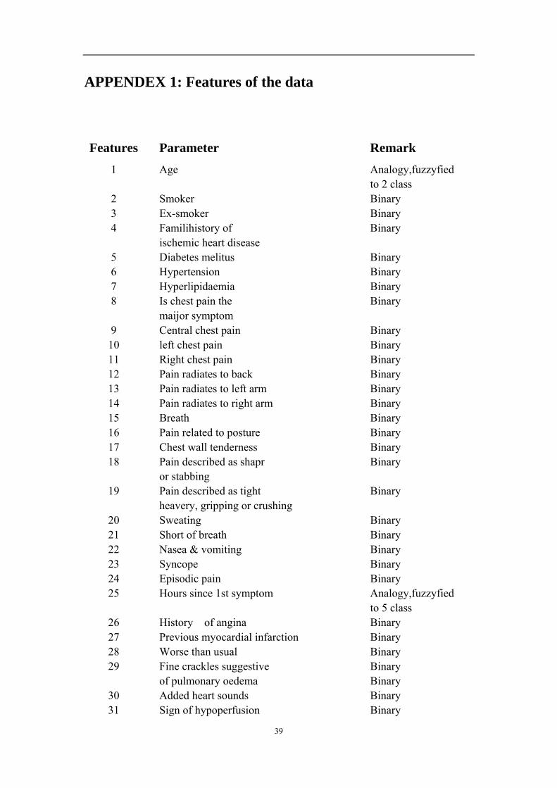
APPENDEX 1: Features of the data

Features Parameter Remark 1 Age Analogy,fuzzyfied to 2 class 2 Smoker Binary 3 Ex-smoker Binary 4 Familihistory of Binary ischemic heart disease 5 Diabetes melitus Binary 6 Hypertension Binary 7 Hyperlipidaemia Binary 8 Is chest pain the Binary maijor symptom 9 Central chest pain Binary 10 left chest pain Binary 11 Right chest pain Binary 12 Pain radiates to back Binary 13 Pain radiates to left arm Binary 14 Pain radiates to right arm Binary 15 Breath Binary 16 Pain related to posture Binary 17 Chest wall tenderness Binary 18 Pain described as shapr Binary or stabbing

19 Pain described as tight Binary heavery, gripping or crushing

20 Sweating Binary 21 Short of breath Binary 22 Nasea & vomiting Binary 23 Syncope Binary 24 Episodic pain Binary 25 Hours since 1st symptom Analogy,fuzzyfied to 5 class

26 History of angina Binary 27 Previous myocardial infarction Binary 28 Worse than usual Binary 29 Fine crackles suggestive Binary of pulmonary oedema Binary

30 Added heart sounds Binary 31 Sign of hypoperfusion Binary

40

32 Rhythm Binary 33 Bundle branch block Binary 34 ST elevation Binary 35 New pathological Q waves Binary 36 Stdep Binary 37 T wave Binary 38 Oldish Binary 39 OldMI Binary 40 Sex Binary

41

APPENDIX 2: Description of Matlab Functions

In this dissertation, all the m-files are run on Matlab 7.0, Release 14, and based on the

Third software, ART & ARTMAP tools which programmed by Aaron Garrett,

Jacksonville State University, website at:

www.Mathworks.com/matlabcentral/fileexchange/

The CD-rom attached to the dissertation contains all relevant m-files which enable to

completion of this dissertation. ART & ARTMAMP tools include two kits which are

used to create, train and test ART and ARTMAP networks respectively.

1. ART tool kit

In this tool kit, function include:

ART_Complement_Code - Complement-codes the given input.

complementCodedData = ART_Complement_Code(data)

ART_Create_Network - Creates the ART network.

net = ART_Create_Network( numFeatures);

where ‘numFeature’ represents the dimension of the input vector.

ART_Activate_Categories - Performs the network category activation for a given

input.

categoryActivation = ART_Activate_Categories(input, weight, bias)

where ‘weight’ is the bottom-up weight matrix of the neural network, ‘bias’ is the

bias parameter, β.

ART_Calculate_Match - Calculates the degree of match between a given input and

a category.

match = ART_Calculate_Match(input, weightVector)

where ‘weightVector’ represents the weight of the winner node in category

42

activate.

ART_Add_New_Category - Adds a new category element to the ART network.

resizedWeight = ART_Add_New_Category(weight)

the added weight has all element of 1.

ART_Update_Weights - Updates the weight matrix of the network.

[updatedWeight, weightChange] = ART_Update_Weights(input, weight,

categoryNumber, learningRate)

where ‘categoryNumber’ is the number of the winner node in F2, ‘learningRate’ is

the learning rate parameter, λ, ‘weightChange’ is used in multi-epoch, whenever

‘weightChange’ change from ‘0’ to ‘1’, the whole train set will be train again until

there is no weight change.

ART_Learn - Trains a given ART network on a dataset.

[new_art_network, categorization] = ART_Learn(art_network, data)

this give a multi-epoch train on the set of ‘data’

ART_Categorize - Uses a trained ART network to categorize a dataset.

categorization = ART_Categorize(art_network, data)

Four of above function are available to user:

ART_Categorize

ART_Complement_Code

ART_Create_Network

ART_Learn

The remained function are used to modularize the structure of the system. These

functions are related to different components of adaptive resonance theory.

‘ART_Activate_Categories’ essentially provides bottom-up activation of the F2 layer

43

for a given input. ‘ART_Add_New_Category’ is used after a series of mismatch resets

in order to create a new F2 neuron to code the current input. ‘ART_Calculate_Match’ is

used to determine the degree of match between a given input and the category coded by

the current F2 neuron. ‘ART_Calculate_Match’is used to update the weight matrix

during learning after resonance has been achieved. The function

‘ART-Complement-Code’, ‘ART_Activate_Categories’, ‘ART_Calculate_Match’

and ‘ART_Calculate_Match’ are also used for ARTMAP models

2. ARTMAP

In this tool kit, the function include:

ARTMAP_Create_Network - Creates the ARTMAP network.

artmap_network = ARTMAP_Create_Network(numFeatures, numClasses)

where ‘numFeature’ and ‘numClass’ are the dimension of input vector and the

number of classes in the problem domain respectively

ARTMAP_Add_New_Category - Adds a new category to the ARTMAP network.

[resizedWeight, resizedMapField] = ARTMAP_Add_New_Category(weight,

mapField)

when a node is added in F2a, a node in map field is also added to respond this node

and relate weight vectors wa and wab will be added as well.

ARTMAP_Learn - Trains a given ARTMAP network on a dataset.

new_artmap_network = ARTMAP_Learn(artmap_network, data, supervisor)

ARTMAP_Classify - Uses a trained ARTMAP network to classify a dataset.

classification = ARTMAP_Classify(artmap_network, data)

‘ARTMAP_Add_New_Category’ function is used to modularize the structure of the

system. And the left functions are available to user.

44

3. User’s application

Data-pretreatment.m – gives the fuzzyfication coding and complements coding，

definite the two-class problem data and three-class data.

cvsystemvalidation.m – gives a 5-fold cross validation for the total data set with

seven vigilance parameters. 10 run of different order of data set are implemented

and the average performance and standard deviation are also calculated.

Onlinevoting2.m – online learning strategy for 2-class problem is implemented in

this function and the average performance curves of ten run with different random

order of data set are plotted as well as the standard deviation for some special

points.

nohotstartsingleonline.m – a online learning of a fuzzy ARTMAP model with 0.1

as the vigilance parameter and with no hot start is implemented with 10 different

order of data run, the average performance curves of ten run with different random

order of data set are plotted as well as the standard deviation for some special

points.

nohotstartvotingonline.m – a voting online strategy with no hot start is implement,

the 15 voter are fuzzy ARTMAP models with different vigilance parameters from

0.05 to 0.75.

onlinevoting3.m – online learning strategy for 3-class problem is implemented in

this function and the average performance curves of ten run with different random

order of data set are plotted as well as the standard deviation for some special

points.

complementtwoclass.m – the data which diagnose to SCP and NCP are classified

by this program with our online learning strategy: with 450 samples of SCP and

650 samples of NCP hot start and 18 voters.

Originaldata.mat – a Matlab data file which contains the original data. It is

employed by data-pretreatment.m.

45

data2a.mat – a Matlab data file which contains the two-class problem. It is

employed by the two-class problem application, onlinevoting.m.

data3a.mat – a Matlab data file which contains the three-class problem. It is

employed by the three-class problem applications.