Embed Size (px)
Citation preview

UQ Engineering
Faculty of Engineering, Architecture and Information Technology
School of Mechanical and Mining Engineering
THE UNIVERSITY OF QUEENSLAND Bachelor of Engineering Thesis
Finite Element Study of the Effects of Characteristic, Geometric
Variables in Handpan Designs and Performance
Student Name: Liam O’DONNELL
Student Number: 42936060
Course Code: MECH4500
Supervisor: Bill Daniel
Submission date: 27th of October, 2017
A project report submitted in partial fulfilment of the requirements of the course: MECH4500
Engineering Thesis

ii
Abstract
Handpans are a recently developed percussive instrument that share similarities with the steel
drum. Current literature has not developed an understanding of how geometry, the only variable
in a handpan, affects performance. Demand currently exceeds productive capacity of the
manufacturers due to the labour intensive nature of building the instrument. Understanding the
system response based on geometry is desired as this may provide insight to the instrument and
improve manufacturability.
An examination of geometric changes on the instrument’s response is the primary concern of
this thesis. Peripheral work represents a large portion of work done and covers the development
of a robust and variable CAD model, testing of actual handpans to determine their harmonic
response and theoretical plate vibration analysis. Key geometric variables are to be identified
and analysed.
An FEA analysis is performed on the CAD model in both modal and transient settings. Results
from the two analysis types are compared. Comparison to actual handpan outputs and
theoretical plate vibrations are also made. Discrepancies are analysed and reasons for differing
output between the instruments in their physical testing are hypothesised.
Non-linear effects are highly significant and current methodologies of modelling need
improvement. Handpans are highly sensitive to geometry and all information generated shows
this. Small changes in geometry create large changes in harmonic response and design details
can alter system output significantly. CAD geometry creation process and model ideology is
sufficient, however, the fidelity of the geometry needs to be, and can be, improved.
Using the recommendations of this report as points of improvement, the current modelling
process should soon be able to accurately and precisely model handpans with very low error.
Once this is the case, fully predictive modelling is possible. At this point a more complete
investigation into the geometry of handpans can be conducted.
iii
Acknowledgements
This year has been interesting and tumultuous, to say the least. A number of people helped me
with this thesis and a number more helped me get through the year.
First and foremost, to Bill; you have been a great supervisor. Whenever I needed anything you
were there with an informative and useful answer. It was never a hassle and you never made it
seem difficult. I would also like to extend my thanks to Belinda, Bill’s wife, whose handpans
were used extensively in this thesis. She was always generous with letting me have them for
study even though she is rather fond of them and they are expensive pieces of equipment.
To Matthew Edwards and David Cusack; without your help and advice this thesis would likely
not have happened. It was good fun spending the odd Friday working in SolidWorks with Matt.
It was equally enjoyable seeing Dave once a week, bouncing ideas off him and learning about
his PhD as he asked about my project.
To Dan Hatch, for providing me with fresh tunes to study to and a good chat every couple of
weeks. International geopolitical tensions to lifting were often discussed, with a side of
University and your mateship helped keep me going. See you Sydney side. And Mitch and
Jesse, you blokes made me appreciate that there is a light at the end of the tunnel.
My girlfriend, Grace Harris; you’ve been really great about my stress and ups and downs.
You’ve helped me get this thesis done and your input is throughout this document. Along with
Mum, Dad and Sarah, you have kept me on track and functioning during this year.
Finally, to Jack, Brendan, Rylie, Steve, Chris, Andy and all the other mates who were always
there for beers when they were needed most; cheers. It has been a hell of a ride. Good luck
getting rid of me, gentlemen.
Thank you.

iv
CONTENTS
1 Introduction ....................................................................................................................... 1
1.1 Motivation ................................................................................................................... 1
1.2 Problem Definition ..................................................................................................... 2
1.3 Scope ........................................................................................................................... 3
1.4 Aims ............................................................................................................................. 3
1.5 Expected Outcomes .................................................................................................... 4
2 Literature Review .............................................................................................................. 5
2.1 Definitions and Analysis Techniques .......................................................................... 5
2.1.1 Natural Frequency and Modes .............................................................................. 5
2.1.2 Damped Natural Frequencies ............................................................................... 7
2.1.3 Finite Element Analysis ....................................................................................... 8
2.1.4 Fast Fourier Transform ....................................................................................... 10
2.1.5 Spectrogram ........................................................................................................ 13
2.1.6 Plate Vibrations .................................................................................................. 15
2.2 Existing Literature ..................................................................................................... 16
2.2.1 Steel Drums ........................................................................................................ 16
2.2.2 Handpans ............................................................................................................ 17
2.3 Summary of Findings ................................................................................................. 20
3 Physical Testing ............................................................................................................... 21
3.1 Introduction ................................................................................................................ 21
3.2 Instrumentation .......................................................................................................... 21
3.3 Methodology .............................................................................................................. 21
3.4 Results ........................................................................................................................ 22
3.5 Discussion .................................................................................................................. 25
4 CAD Model ..................................................................................................................... 26
4.1 Introduction ................................................................................................................ 26
4.2 Development of Methodology ................................................................................... 26
4.3 Outcomes ................................................................................................................... 27
4.4 Further Work .............................................................................................................. 29
4.4.1 3D Scan .............................................................................................................. 29
4.4.2 Other Instruments ............................................................................................... 30
4.5 Discussion and Recommendations ............................................................................ 30
5 Theoretical Analysis ........................................................................................................ 31

v
5.1 Introduction ................................................................................................................ 31
5.2 Pi Drum Measurements ............................................................................................. 31
5.2.1 Rectangular Plates .............................................................................................. 32
5.2.2 Circular Plates .................................................................................................... 33
5.2.3 Annular Plates .................................................................................................... 34
5.3 Discussion .................................................................................................................. 35
6 FEA Analysis ................................................................................................................... 37
6.1 Introduction ................................................................................................................ 37
6.2 Modal Analysis .......................................................................................................... 37
6.2.1 Method and Set-Up ............................................................................................. 37
6.2.2 Results ................................................................................................................ 37
6.3 Transient Analysis ..................................................................................................... 39
6.3.1 Method and Set Up ............................................................................................. 39
6.3.2 Results ................................................................................................................ 39
6.4 Discussion .................................................................................................................. 41
7 Geometric Effects ............................................................................................................ 42
7.1 Introduction ................................................................................................................ 42
7.2 Method ....................................................................................................................... 42
7.3 Results ........................................................................................................................ 43
7.3.1 All Notes Modal ................................................................................................. 43
7.3.2 D5 Note Analysis ............................................................................................... 44
7.4 Discussion .................................................................................................................. 45
8 Discussion ........................................................................................................................ 46
9 Conclusions and recommendations ................................................................................. 48
9.1 Conclusions ................................................................................................................ 48
9.2 Recommendations ...................................................................................................... 49
10 References ....................................................................................................................... 51
11 Appendices ...................................................................................................................... 54
11.1 Appendix A ............................................................................................................ 54
11.1.1 Analytical Rectangular Plate Solution Coefficients ........................................... 54
11.1.2 Analytical Circular Plate Solution Coefficients ................................................. 56
11.1.3 Analytical Annular Plate Solution Coefficients ................................................. 57
11.2 Appendix B ............................................................................................................ 58
11.2.1 Matlab Code for Audio Sample Analysis ........................................................... 58
11.2.2 Tables of Observations of Physical Testing ....................................................... 59

vi
11.2.3 Pi Drum Spectrograms ....................................................................................... 63
11.2.4 Meridian Spectrograms....................................................................................... 71
11.3 Appendix C ............................................................................................................ 79
11.4 Appendix D ............................................................................................................ 85
11.4.1 Modal Analysis Method ..................................................................................... 85
11.4.2 Transient Analysis Method ................................................................................. 89
11.4.3 Transient Analysis FFTs ..................................................................................... 92
11.5 Appendix E ............................................................................................................. 96
List of Figures
Figure 1: Handpans Being Played ((Paniverse 2017)) ............................................................... 1
Figure 2: Vibration of a Cantilever Beam (ICT 2017) ............................................................... 7
Figure 3: Example FFT ............................................................................................................ 12
Figure 4: Mirror Around Nyquist Frequency ........................................................................... 12
Figure 5: Spectrogram with 1024 ............................................................................................. 14
Figure 6: Spectrogram with 4096 ............................................................................................. 14
Figure 7: Holographic Image of Top Ding Mode Shape (Rossing, Morrison et al. 2007)....... 18
Figure 8: Holographic Image of F Note Mode Shape (Rossing, Morrison et al. 2007) ........... 19
Figure 9: Cake Slice View ........................................................................................................ 27
Figure 10: D4 Note Cake Slice – Isometric View .................................................................... 28
Figure 11: Completed CAD Model - Top View ....................................................................... 28
Figure 12: 3D Scan - Pi Drum .................................................................................................. 29
Figure 13: Meridian Handpan................................................................................................... 30
Figure 14: Rectangular Plate Results - Line Graph .................................................................. 33
Figure 15: Circular Plate Results .............................................................................................. 34
Figure 16: Annular Plate Results .............................................................................................. 35
Figure 17: Example Modal Result ............................................................................................ 38
Figure 18: FFT of A4 Note ....................................................................................................... 40
Figure 19: Transient, Modal and Measured Results Line Graph ............................................. 41
Figure 20: Differing Geometric Effects - Modal Analysis ....................................................... 43
Figure 21: D5 Note - Modal vs Transient Geometric Effects .................................................. 44
Figure 22: Rectangular Plate Boundary Condition Constants .................................................. 54
Figure 23: Rectangular Plate Boundary Condition Constants Continued ................................ 55
Figure 24: Clamped Circular Plate Boundary Condition Constants ........................................ 56
Figure 25: Simply Supported Circular Plate Boundary Condition Constants .......................... 56
Figure 26: Clamped Annular Plate Boundary Condition Constants ........................................ 57
Figure 27: Simply Supported Annular Plate Boundary Condition Constants .......................... 57
Figure 28: Audio Sample Analysis Matlab Code ..................................................................... 58
Figure 29: Pi Drum - D4 Spectrogram – No Stand .................................................................. 63
Figure 30: Pi Drum - D4 Spectrogram - Stand ......................................................................... 63
Figure 31: Pi Drum - E4 Spectrogram – No Stand ................................................................... 64

vii
Figure 32: Pi Drum - E4 Spectrogram – Stand ......................................................................... 64
Figure 33: Pi Drum - F4 Spectrogram – No Stand ................................................................... 65
Figure 34: Pi Drum - F4 Spectrogram – Stand ......................................................................... 65
Figure 35: Pi Drum - G4 Spectrogram – No Stand .................................................................. 66
Figure 36: Pi Drum - G4 Spectrogram – Stand ........................................................................ 66
Figure 37: Pi Drum - A4 Spectrogram – Stand ........................................................................ 67
Figure 38: Pi Drum - A4 Spectrogram – No Stand .................................................................. 67
Figure 39: Pi Drum - Bb4 Spectrogram – Stand ...................................................................... 68
Figure 40: Pi Drum - Bb4 Spectrogram – No Stand ................................................................ 68
Figure 41: Pi Drum - C5 Spectrogram – Stand ........................................................................ 69
Figure 42: Pi Drum – C5 Spectrogram – No Stand .................................................................. 69
Figure 43: Pi Drum – D5 Spectrogram – No Stand .................................................................. 70
Figure 44: Pi Drum – D5 Spectrogram – Stand ....................................................................... 70
Figure 45: Meridian – G3 Spectrogram – Stand ...................................................................... 71
Figure 46: Meridian – G3 Spectrogram – No Stand ................................................................. 71
Figure 47: Meridian – Ab3 Spectrogram – No Stand ............................................................... 72
Figure 48: Meridian – Ab3 Spectrogram – Stand .................................................................... 72
Figure 49: Meridian – C4 Spectrogram – No Stand ................................................................. 73
Figure 50: Meridian – C4 Spectrogram – Stand ....................................................................... 73
Figure 51: Meridian – Eb4 Spectrogram – No Stand ............................................................... 74
Figure 52: Meridian – Eb4 Spectrogram – No Stand ............................................................... 74
Figure 53: Meridian – F4 Spectrogram – No Stand ................................................................. 75
Figure 54: Meridian – F4 Spectrogram – Stand ....................................................................... 75
Figure 55: Meridian – G4 Spectrogram – No Stand ................................................................. 76
Figure 56: Meridian – G4 Spectrogram – Stand ...................................................................... 76
Figure 57: Meridian – Bb4 Spectrogram – No Stand ............................................................... 77
Figure 58: Meridian – Bb4 Spectrogram – Stand ..................................................................... 77
Figure 59: Meridian – C5 Spectrogram – No Stand ................................................................. 78
Figure 60: Meridian – C5 Spectrogram – Stand ....................................................................... 78
Figure 61: Shell Sketch Bottom ............................................................................................... 79
Figure 62: Shell Sketch Top ..................................................................................................... 80
Figure 63: Two Way Revolve .................................................................................................. 80
Figure 64: Die ........................................................................................................................... 81
Figure 65: Die Push .................................................................................................................. 81
Figure 66: Flattening Die .......................................................................................................... 82
Figure 67: Dimple Indent ......................................................................................................... 83
Figure 68: Slice Construction Lines ......................................................................................... 83
Figure 69: Modal Project Tree Overview ................................................................................. 85
Figure 70: Mesh Sweep Method for Solid Shell Elements ...................................................... 86
Figure 71: FEA Contact Region Definition .............................................................................. 86
Figure 72: Mesh Refinement .................................................................................................... 87
Figure 73: Support for FEA ...................................................................................................... 87
Figure 74: Analysis Settings ..................................................................................................... 88
Figure 75: FEA Modal Results ................................................................................................. 88
Figure 76: Named Selections .................................................................................................... 89
viii
Figure 77: Nodal Force ............................................................................................................. 90
Figure 78: Transient Analysis Settings ..................................................................................... 90
Figure 79: Nodal Displacement Time History ......................................................................... 90
Figure 80: FFT of Transient Analysis Time History - D4 ........................................................ 92
Figure 81: FFT of Transient Analysis Time History - E4 ........................................................ 92
Figure 82: FFT of Transient Analysis Time History - F4 ........................................................ 93
Figure 83: FFT of Transient Analysis Time History - G4 ........................................................ 93
Figure 84: FFT of Transient Analysis Time History - A4 ........................................................ 94
Figure 85: FFT of Transient Analysis Time History - Bb4 ...................................................... 94
Figure 86: FFT of Transient Analysis Time History - C5 ........................................................ 95
Figure 87: FFT of Transient Analysis Time History - D5 ........................................................ 95
Figure 88: FFT - D5 - No Dimple ............................................................................................ 96
Figure 89: FFT- D5 - Double Thickness .................................................................................. 96
Figure 90: FFT - D5 - Double AR ............................................................................................ 97
Figure 91: FFT - D5 - Raised ................................................................................................... 97
Figure 92: FFT - D5 - Double AR No Dimple ......................................................................... 97
Figure 93: FFT - D5 - Half AR ................................................................................................ 97
Figure 94: FFT - D5 - Half AR No Dimple .............................................................................. 97
List of Tables
Table 1: Pi Drum Tested Modal Frequencies ........................................................................... 22
Table 2: Meridian Tested Modal Frequencies .......................................................................... 23
Table 3: Pi Drum Critical Note Dimensions ............................................................................ 31
Table 4: Pi Drum Variables ...................................................................................................... 32
Table 5: Analytical Solutions - Rectangular Plate.................................................................... 32
Table 6: Analytical Solutions - Circular Plate .......................................................................... 33
Table 7: Analytical Solutions - Annular Plate .......................................................................... 35
Table 8: Modal Analysis Frequencies ...................................................................................... 38
Table 9: Transient, Modal and Measured Frequencies............................................................. 40
Table 10: All Notes Geometric Effects .................................................................................... 43
Table 11: D5 Note - Modal and Transient Analysis ................................................................. 44
Table 12: FFT, Spectrogram and Power Response Observations - Pi Drum No Stand ........... 59
Table 13: FFT, Spectrogram and Power Response Observations - Pi Drum Stand ................. 60
Table 14: FFT, Spectrogram and Power Response Observations - Meridian No Stand .......... 61
Table 15: FFT, Spectrogram and Power Response Observations - Meridian Stand ................ 62

1
1 INTRODUCTION
1.1 Motivation
Handpans (Figure 1) are a relatively new percussive musical instrument with increasing usage
(Google 2017) since its invention in 2000 (Rohner and Schärer 2007). Basic designs are a
conical shell with small idents or raised sections around the circumference of the shell. These
indents are tuned so as to vibrate locally when struck, producing notes of a specific tone and
scale. Current design and manufacture rely on a guess and check method (Morrison and Rossing
2007, Rohner and Schärer 2007). Comparing the effects of design changes to develop an
understanding of the instrument workings is desired, as well as the generation of working digital
models.
Notes, and thus the musical scale, on a handpan are restricted by the number of indents that can
fit around the circumference. The notes are also limited by the mode of vibration that an indent
can operate in. Furthermore, the vibration of one indent (or note) can interfere with its
Figure 1: Handpans Being Played ((Paniverse 2017))
2
neighbours if not adequately spaced and this is often the limiting design factor (Rossing,
Morrison et al. 2007).
Many manufacturers use different geometries of the shell and indents to unknown effect. To
understand why a manufacturer might use a rotated ellipse shape instead of a hemisphere, for
example, is a primary motivator. Essentially, the author and supervisor are curious as to the
why and how of manufacturing these fascinating new instruments.
1.2 Problem Definition
Design and build methodology of handpans is heavily guess and check, with only a limited
number of investigations delving into theoretical modelling. Design elements such as indent
spacing, size and orientation are highly dependent on the individual manufacturer of the
handpan. Consistent classification of design parameters and why they are used is not available
and the effect of most possible changes in design is not known (a brief example would be the
elliptical indents provided by some manufacturers). Rigour in classifying and predicting the
effects of design changes is the end goal of this project.
The function of finite element analysis (FEA) is to examine structures computationally and
learn their predicted behaviour in real life. FEA allows us to alter designs quickly and easily
via a computer aided design (CAD) tool to observe changes to the structure. This method can
sometimes be limited if the manufacture of the structure is not consistent. Thus a test of real
response of a handpan and a comparison to a FEA model will be needed to validate the
FEA/CAD model.
Spectral analysis via MATLAB of an existing handpan provides the start point of investigations.
From here it is hoped that an ANSYS FEA model of the existing pan can be created that mimics
the response of the real pan. Once this meeting of physical and digital performance is achieved
the ANSYS model can be modified and experimented with. Ultimately, the effects of changing
the design (geometry) of the handpan and classifying the outcomes may be achieved. This lively

3
instrument may become far more prevalent if consistent performance of the product can be
predicted and ensured. This project strives for that goal.
1.3 Scope
Currently the project runs two aspects simultaneously; the testing of the physical handpan and
subsequent spectral analysis and the development of a theoretical model to examine the effects
of changing the handpan design. The physical testing will aim to provide consistent data
gathering and analysis techniques while the theoretical model will test variation of parameters
that is not possible with the physical handpan. Physical testing also provides baseline
information that can help inform the theoretical model analysis.
Desired lines of enquiry for the physical testing include developing consistent striking and
sound recording methods. Theoretical model scope includes analysing the effect of geometric
changes to the handpan.
1.4 Aims
Primary project goals:
1) Produce a repeatable method of testing the output of a physical handpan. This will
include methods of measuring the sound, striking the pan and supporting the pan.
Spectral analysis of the results will form a key part of this goal.
2) Develop a validated FEA model of the existing handpan that can provide a spectral
vibratory response equivalent to the real device. Comparison of measured notes and
their spectral response will be compared with the ANSYS model response and spectral
output.
3) Use CAD and FEA to determine the effect of each design parameter on the output of
the handpan. This will involve altering the CAD model, once it has been validated, and
testing its spectral response for a standardised strike input. An ability to design a
handpan based on theory to produce a certain note or scale would be an end goal.
4
1.5 Expected Outcomes
The following list outlines the desired outcomes of the project.
1) Develop a standard test procedure for analysing the resonant response of the hand pan
when struck.
2) Identify and categorise any discrepancy between physical handpan and ANSYS model
responses.
3) Understand the effects of each design element of a handpan and how altering these
elements affects performance.
4) Suggest methods for achieving desired notes or handpan performance based on
theoretical design.
5) Suggestions for further work.

5
2 LITERATURE REVIEW
The literature review comprises of two primary sections; Definitions and Analysis Techniques
and Existing Literature. Definitions and Analysis Techniques is broken into multiple
subsections comprising: Natural Frequencies and Modes, Damped Natural Frequencies, Finite
Element Analysis, Fast Fourier Transform, Spectrograms and Plate Vibrations. Existing work
examines Steel Pan and Handpan literature. The Definitions and Analysis Techniques segment
draws on the academic works evaluated in the Existing Literature section. A Summary of
Findings is provided to close out the review.
2.1 Definitions and Analysis Techniques
2.1.1 Natural Frequency and Modes
Natural frequency is the rate of oscillation of an unforced (free vibration) object. It is an inherent
property of all physical objects and is affected by factors such as material type, geometry,
boundary conditions and temperature. Each degree of freedom an object possesses corresponds
to a natural frequency in radians per second denoted by ωn, where subscript n represents the
degree of freedom. This degree of freedom is called a mode and the way it vibrates is called its
mode shape. Therefore, each natural frequency has a corresponding mode of vibration with a
defined shape (Rao 2011).
ωn (rad s-1) is sometimes called the circular natural frequency and fn (Hz) is called the natural
frequency. The two are related via:
𝑓𝑛 =𝜔𝑛
2𝜋
Where:
𝑓𝑛 = natural frequency in Hertz (Hz),
𝜔𝑛 = natural frequency, or circular natural frequency, in radians per second (rad/s) and,

6
𝜋 is the geometric constant (approximately 3.14).
Certain modes of natural vibration can be excited by applying an impulse to an object. Based
on where and how this impulse is applied, particular (already existing) natural modes of
vibration, at their corresponding natural frequencies, can be made to oscillate. These modes
have points called nodes, denoted by N, which are points of zero motion when that mode has
been excited. Conversely, anti-nodes are points of maximum oscillation displacement under a
given mode (Rao 2011) . Applying an impulse to a node of a mode will not excite that mode to
oscillation. However, applying the same impulse to an anti-node will achieve the maximum
excitation of that mode.
Figure 2 shows the first three modes of vibration for a cantilever beam of length (L), mass (m),
second moment of area (I) (which is a geometric property of the beam cross section) and elastic
modulus (E), which is an inherent material property that measures stiffness. Part (b), (c) and
(d) of the figure show the first, second and third modes respectively with part (a) showing the
beam setup. The analytical solution for the corresponding natural frequency is presented next
to each mode.
A load or impulse applied at N1 in part (c) of Figure 2 will not excite the second mode of
vibration. Mode 2 has an anti-node is roughly hallway between the fixed support and N1, and
an impulse applied here would excite the mode to the fullest capability of the impulse, at
frequency ω2.

7
Methods for calculating natural frequency can be analytical or numerical, but for complex
geometries it is found numerically. This is often performed by FEA packages. In physical
systems it is measured, as in Morrison’s paper which used holographic interferometry to analyse
the first three modes of vibration of each note (Morrison and Rossing 2007). Even more simply,
if the system generates a sound, this can be recorded by microphone and analysed to determine
frequencies of modes present following excitation (Alon 2015).
2.1.2 Damped Natural Frequencies
A natural frequency can be damped or undamped depending on the amount of damping present
in the system. This is often the most difficult part of a system to determine; where the damping
is, how much is present and what types of damping are present (Rao 2011). Natural frequencies
Figure 2: Vibration of a Cantilever Beam (ICT 2017)
8
of a system are largely unaffected by low levels of damping. However, if a system is what is
known as critically damped or overdamped the natural frequency cannot occur. Existing studies
on handpans and steel drums have not found damping to be considerably high and it is known
these systems do vibrate readily (Achong 1996, Morrison and Rossing 2007, Rohner and
Schärer 2007, Rossing, Morrison et al. 2007).
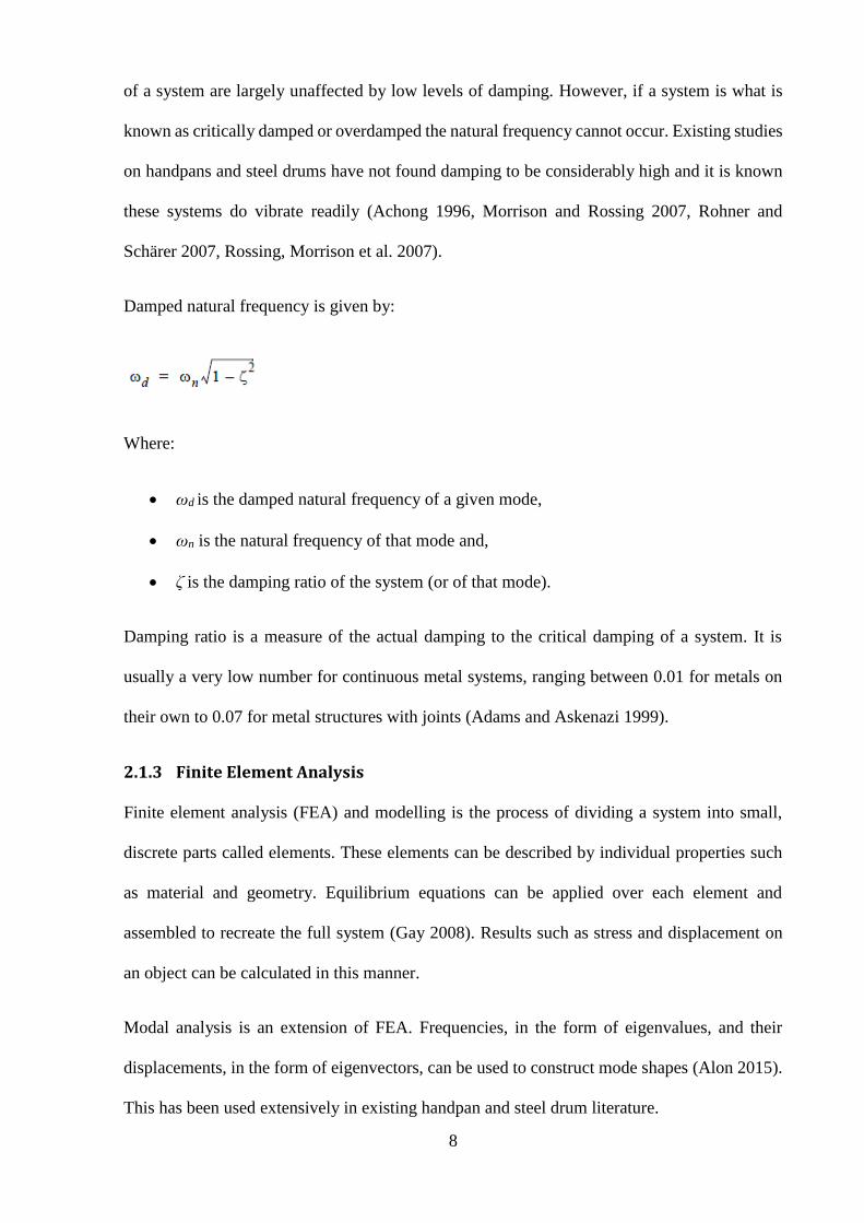
Damped natural frequency is given by:
Where:
ωd is the damped natural frequency of a given mode,
ωn is the natural frequency of that mode and,
ζ is the damping ratio of the system (or of that mode).
Damping ratio is a measure of the actual damping to the critical damping of a system. It is
usually a very low number for continuous metal systems, ranging between 0.01 for metals on
their own to 0.07 for metal structures with joints (Adams and Askenazi 1999).
2.1.3 Finite Element Analysis
Finite element analysis (FEA) and modelling is the process of dividing a system into small,
discrete parts called elements. These elements can be described by individual properties such
as material and geometry. Equilibrium equations can be applied over each element and
assembled to recreate the full system (Gay 2008). Results such as stress and displacement on
an object can be calculated in this manner.
Modal analysis is an extension of FEA. Frequencies, in the form of eigenvalues, and their
displacements, in the form of eigenvectors, can be used to construct mode shapes (Alon 2015).
This has been used extensively in existing handpan and steel drum literature.

9
An FEA package extracts this information using the underlying method of its solving
algorithms. A simple, single degree of freedom system with no damping and no applied loading
has the following matrix form equation of motion (EoM):
[𝑀]{𝑢}̈ + [𝐾]{𝑢} = 0
Where:
[M] = the mass matrix of the system,
[K] = the stiffness matrix of the system,
{𝑢} = the displacement vector of the system,
{𝑢}̈ = the acceleration vector (second derivative of displacement) of the system.
This matrix form the EoM for undamped free vibration. Assuming a harmonic solution to the
displacement of form:
{𝑢} = {𝜙}sin𝜔𝑡
Where:
{𝜙} = the eigenvector or mode shape.
Differentiating Equation X twice and then substituting the result and the original function into
Equation Y yields:
−𝜔2[𝑀]{𝜙}𝑠𝑖𝑛𝜔𝑡 + [𝐾]{𝜙}𝑠𝑖𝑛𝜔𝑡 = 0
Which simplifies to:
([𝐾] − 𝜔2[𝑀]){𝜙} = 0
This is now in the form of the eigenequation. More often this is shown in the form:
[𝐴 − 𝜆𝐼]𝑋 = 0

10
Where:
A = square matrix,
λ = eigenvalues,
I = identity matrix,
X = eigenvector.
Thus, when written in terms of K, ω, and M the eigenequation is the physical representation of
natural frequencies and mode shapes of a system, with 𝜔2 = 𝜆. Analytically, the eigenequation
is solved using the determinant of ([𝐾] − 𝜔2[𝑀])to solve for each 𝜔𝑖2 and then solve for each
mode shape (Software 2011). Numerically, it is solved by iteration on an initial guess of the
eigenvectors.
FEA packages can perform this analysis for complex systems and limit their solution space to
minimise computation time. Thus, for large and complex systems, early modes of vibration and
their natural frequencies can be extracted.
2.1.3.1 Transient Analysis
Transient dynamic analysis is a technique used to determine the dynamic response of a structure
under time-dependent loads. Sometimes, this is called time-history analysis or transient
structural analysis. Under standard static structural analysis or modal analysis, time dependent
effects and non-linearities are not accounted for. These include inertial effects, which are often
significant in thin membrane structures (Han and Petyt 1997), geometric stiffness
considerations or changing load over time.
2.1.4 Fast Fourier Transform
Once a recording of a vibrating has occurred, be it acoustically, via accelerometer or optically,
analysis of frequencies present is essential. Fourier transforms are used to do this. Fourier
transforms are found by:

11
X(f) is the Fourier transform of the time domain signal, x(t), and f is the frequency (Rao 2011).
Most commonly a fast Fourier transform (FFT) is used to do this. It separates time series data
into the frequency domain, allowing the dominant frequencies present to be identified. It is
inherently a numerical method performed on discrete data points and this transform is called
the discrete Fourier transform (DFT), of which an FFT is an efficient method of computation
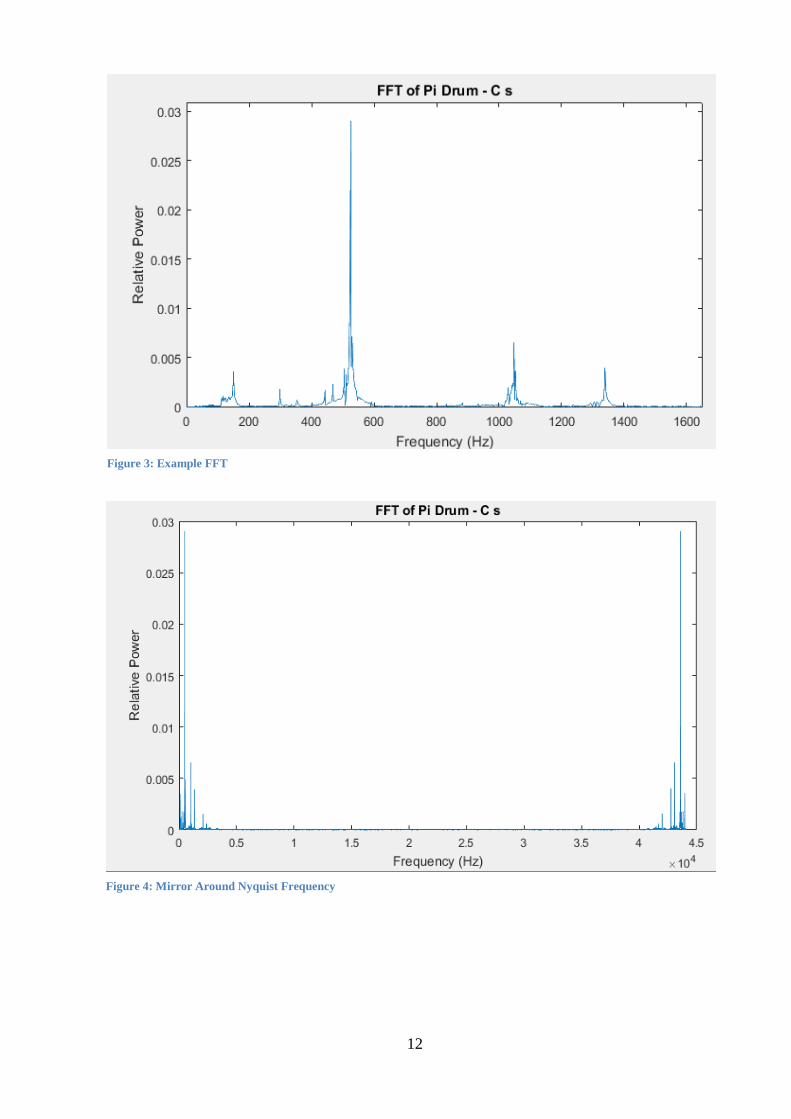
(Alon 2015). Figure 3 shows an example FFT of the C note on the PiDrum handpan with peaks
in relative power at dominant frequencies. The primary spike corresponds to 523 Hz, the
expected pitch of C5.
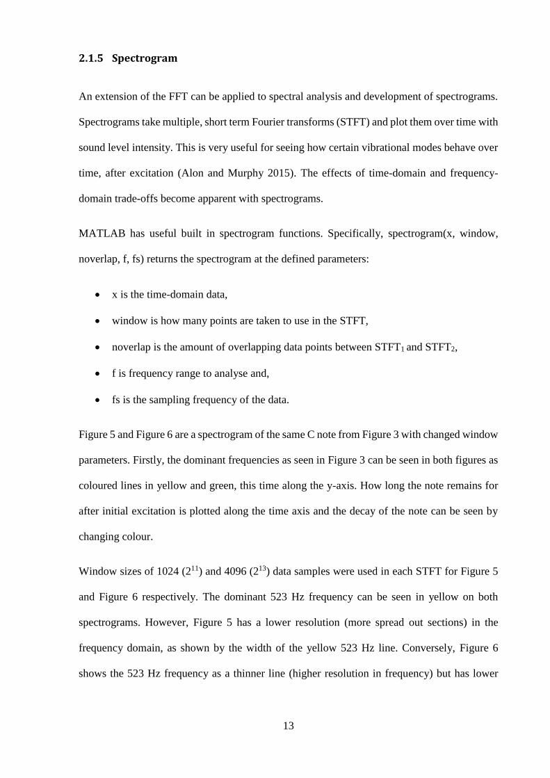
This method has some limitations. Namely, the Nyquist frequency, which is the equal to half
the sampling frequency. This means that frequencies over half of the sampling frequency cannot
be identified. Frequencies above the Nyquist frequency will be displayed but will be a mirror
of those below the Nyquist, with the Nyquist frequency being the plane of symmetry. Figure 4
shows the mirror effect, the Nyquist frequency in this case is 24 kHz with sample rate 48 kHz.
Thus a sufficient sampling frequency must be present. However, this is complicated by the
inverse relation between sampling frequency and sampling time gap. Thus there is always a
trade-off between time-domain and frequency-domain resolution (Achong 1996).
12
Figure 3: Example FFT
Figure 4: Mirror Around Nyquist Frequency
13
2.1.5 Spectrogram
An extension of the FFT can be applied to spectral analysis and development of spectrograms.
Spectrograms take multiple, short term Fourier transforms (STFT) and plot them over time with
sound level intensity. This is very useful for seeing how certain vibrational modes behave over
time, after excitation (Alon and Murphy 2015). The effects of time-domain and frequency-
domain trade-offs become apparent with spectrograms.
MATLAB has useful built in spectrogram functions. Specifically, spectrogram(x, window,
noverlap, f, fs) returns the spectrogram at the defined parameters:
x is the time-domain data,
window is how many points are taken to use in the STFT,
noverlap is the amount of overlapping data points between STFT1 and STFT2,
f is frequency range to analyse and,
fs is the sampling frequency of the data.
Figure 5 and Figure 6 are a spectrogram of the same C note from Figure 3 with changed window
parameters. Firstly, the dominant frequencies as seen in Figure 3 can be seen in both figures as
coloured lines in yellow and green, this time along the y-axis. How long the note remains for
after initial excitation is plotted along the time axis and the decay of the note can be seen by
changing colour.
Window sizes of 1024 (211) and 4096 (213) data samples were used in each STFT for Figure 5
and Figure 6 respectively. The dominant 523 Hz frequency can be seen in yellow on both
spectrograms. However, Figure 5 has a lower resolution (more spread out sections) in the
frequency domain, as shown by the width of the yellow 523 Hz line. Conversely, Figure 6
shows the 523 Hz frequency as a thinner line (higher resolution in frequency) but has lower

14
resolution in the time domain, as shown by the width of the individual segments while moving
along the time axis.
Figure 6: Spectrogram with 4096
Figure 5: Spectrogram with 1024
15
2.1.6 Plate Vibrations
Analytical solutions exist for plate vibrations under various boundary conditions (Leissa 1969,
Leissa 1973, Shi, Shi et al. 2014). Simplest solutions involve using tables of values and
prescribed equations.
2.1.6.1 Rectangular Plates
A brief overview of important rectangular plate equations of interest follows.
For a rectangular plate of constant thickness the following equation describes the natural
frequency (Leissa 1969):
𝜔2 =𝜋4𝐷
𝑎4𝜌
𝐾
𝑁
Where:
a = length of the plate (m)
𝜌 = density (𝑘𝑔
𝑚3)
K = constant from Figure 22 that depends on aspect ratio of plate and boundary
conditions
N = constant from Figure 22 that depends on boundary conditions
𝐷 =𝐸ℎ3
12(1−𝜈2)
h = thickness of plate (m)
ν = Poisson’s ratio of material
Figure 22 (contained in Appendix A) in Leissa’s 1969 paper for NASA contains the boundary
conditions and relevant K and N values for that condition. Aspect ratio (the ratio of length to
width) is an important variable. If the width of a plate is denoted b then aspect ratio is a/b.
16
2.1.6.2 Circular Plates and Annular Plates
Leissa presents tables of critical values of a constant called 𝜆2 for the various possible modes
of circular and annular plate vibrations with varying boundary conditions (Appendix A).
Relationship between variables already established for circular and annular plates is:
𝜆2 = ω𝑎2√𝜌
𝐷
Where:
𝜆2is a constant found in various tables from Leissa (Appendix A),
𝑎is the plate outer radius.
In tables values for 𝜆2 are presented for various values of n and s. These constants are not
important for the purposes of this paper as they are both taken to be zero.
Annular plates have one further variables which is b/a, where b is the inner radius of the
annulus. Interpolation between the presented b/a values would be required as they are not
presented to a high resolution.
2.2 Existing Literature
2.2.1 Steel Drums
Much informative ground work has been performed on the steel drum, a father to the handpan.
“The steelpan as a system of non-linear mode-localized oscillator” part 1(Achong 1996) and
part 2 (Achong and Sinanan-Singh 1997) represent the most rigorous mathematical analysis of
the steel drum. Much of the theory utilised and presented in these papers forms a basis of
theories of interaction for the investigation; specifically, the use of STFT to analyse frequency
domain data from time-domain information alone.

17
Significant effort was undertaken by Achong to look at the interactions and bifurcations of the
steel drum system. One key point of the Achong papers was to show, with rigour, that coupling
of notes is not a large consideration and analysis of the system can be done as a single note
analysis, if natural frequencies are not very close to each other. While the coupling of modes
and mathematical predictions are interesting and, in some regards, useful, it does not help
answer the central question of this paper. It does, however, provide some insight into the
complexities of systems with limited geometry and their interactions.
“Nonlinear vibrations of steelpans: analysis of mode coupling in view of modal sound
synthesis” (Monteil, Touzé et al. 2013), is one paper to examine the sue of FEA in analysing
the steel drum. Importantly, it rigorously identifies the need to examine non-linear effects when
analysing the steel drum. It does not examine the effects of changing geometry, merely how to
effectively model an existing geometry. One final point is the alignment of theoretical and
physical results was a strong focus of the paper. This is of note because it is perhaps the only
paper to attempt to correlate the two with accuracy and precision. Full correlation of the two is
not achieved as there are some discrepancies but, overall, the trend of the physical system was
able to be predicted by the theory.
These two papers are the most informative and other works build on their basis without much
extension.
2.2.2 Handpans
“Modes of vibration and sound radiation from hang” (Morrison and Rossing 2007) focuses
exclusively on measurement of the modes of vibration and natural frequencies, including
visualisation in the form of holographic interferometry. Holographic interferometry projects
light onto the surface of a vibrating objects and the resulting phase shifts in light caused by the
movement of the surface can be detected by a received and displayed. Images using this method
visualise vibrational modes with great accuracy and provide a method for comparing theoretical
18
model modes to tested, existing modes, of a similar instrument. Other similar works (Rohner
and Schärer 2007, Rossing, Morrison et al. 2007) help provide direction for physical testing but
report no work on changing geometry.
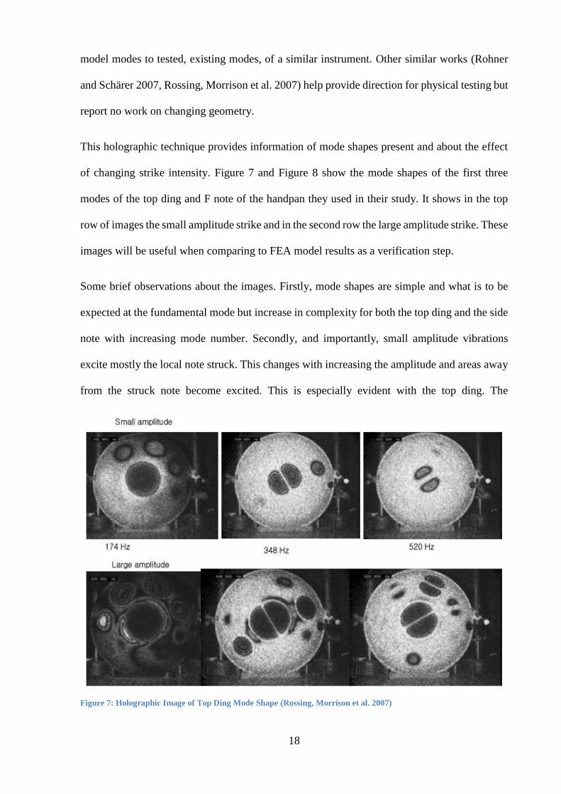
This holographic technique provides information of mode shapes present and about the effect
of changing strike intensity. Figure 7 and Figure 8 show the mode shapes of the first three
modes of the top ding and F note of the handpan they used in their study. It shows in the top
row of images the small amplitude strike and in the second row the large amplitude strike. These
images will be useful when comparing to FEA model results as a verification step.
Some brief observations about the images. Firstly, mode shapes are simple and what is to be
expected at the fundamental mode but increase in complexity for both the top ding and the side
note with increasing mode number. Secondly, and importantly, small amplitude vibrations
excite mostly the local note struck. This changes with increasing the amplitude and areas away
from the struck note become excited. This is especially evident with the top ding. The
Figure 7: Holographic Image of Top Ding Mode Shape (Rossing, Morrison et al. 2007)

19
fundamental mode of the F note at 368 Hz excites the top ding when struck with large amplitude
which has a resonance at 348 Hz, more than 5% different.
“Analysis and Synthesis of the Handpan Sound” (Alon 2015), represents the most complete
body of work on analysing handpan response to changing input factors. This single paper
informs much of the current analysis. Primarily this paper was focused on testing and analysis
of the physical system, with no digital modelling performed. No investigation of changing
geometry, with the exception of entirely changing the instrument was made. While rigorous,
methodical and a complete study, it does not provide much of the insight the author craves.
To date, no work has been found investigating the geometric effects of the handpan on note
generation. Similarly, no work has been found that focuses on handpan design before
manufacture or the ability to produce handpans industrially instead of by hand. Existing works
focus on the measurement of physical systems and the methods of analysing these systems.
Figure 8: Holographic Image of F Note Mode Shape (Rossing, Morrison et al. 2007)

20
2.3 Summary of Findings
Existing literature focuses heavily on steel drums, as opposed to handpans. Current literature
on both, however, does not examine the effects of changing geometry, even though use of FEA
models can be seen. Furthermore, literature on handpans themselves is limited to a few articles
and the very useful thesis by (Alon 2015). Methods of analysing both physical and digital
systems, as well as data gathered from both, has comprehensively been presented. Three options
are presented for validating results; physical testing, theoretical plate vibration solutions and
digital modelling via FEA. Usage of the FFT is key to analysis of data from the physical testing
and transient analysis of the system.
Despite claims on the contrary from papers, modal interactions appear to be significant as
shown by Figure 7 and Figure 8. Non-linear effects and modal interactions are exacerbated by
increasing the amplitude of vibration (which is expected) and this may provide a significant
point of interest.
21
3 PHYSICAL TESTING
3.1 Introduction
Acquiring data on the actual instruments available and developing a methodology for attaining
accurate and consistent results are a project requirement and goal respectively. Data for both
the Meridian and Pi Drum handpans was gathered for each note as well as for the instrument
being on or off a stand. Originally, a tool to deliver a consistent strike to the instrument was to
be created. However, this produced inconsistent and artificially high pitched notes and so was
abandoned.
3.2 Instrumentation
The following is required:
1. Handpan (two varieties were available; the Meridian and the Pi Drum)
2. Microphone
3. Audio Recording Software
4. Portable device for recording (laptop or phone)
5. Stand for instrument
6. Some cloth to sit under the instrument
7. Anechoic chamber
8. Index finger
3.3 Methodology
A brief methodology is presented.
1. Place the handpan in the middle of the anechoic chamber either on the stand or on a
piece of cloth.
2. Place the microphone on the floor about 30cm away from the note being struck.

22
3. Keep the mobile device close to the microphone for access.
4. Perform a few test strikes with finger until a “good” sounding note is achieved (that is,
not off note or with discrepancies).
5. Begin recording the audio and immediately strike the desired note. Wait until it has
faded away entirely and stop recording.
6. Play note back to ensure no noise pollution has entered the recording.
7. Save note using a specific naming convention (the author used the name of the
instrument, the note and if it was on or off the stand).
8. Repeat steps 2 to 7 for all notes on the instrument.
9. Change the instrument from stand to floor or vice versa and repeat steps 2 to 8.
10. Change instruments and repeat steps 2 to 9.
11. Use the code in Appendix B (Figure 28) to analyse the data.
3.4 Results
Table 1 and Table 2 contain the measured and expected values for the first, second and third
modal frequencies for each note for each instrument respectively. The percentage error is also
presented. Appendix B contains the Spectrograms (Figure 29 to Figure 60) for each note on
each instrument; both on and off a stand. A list of observations along with the raw data for each
note is also presented in Appendix B (Table 12 to Table 15).
Table 1: Pi Drum Tested Modal Frequencies
Tested Modal Frequencies for Pi Drum With and Without Stand
Note No Stand Stand
Mode Number 1 2 3 1 2 3
D4 Measured (Hz) 297.9 - 884.8 294.3 588.3 884.4
Expected (Hz) 293.66 587.32 880.98 293.66 587.32 880.98
% Error -1.42% - -0.43% -0.22% -0.17% -0.39%

23
E4 Measured (Hz) 335.2 662.2 - 333 662.4 -
Expected (Hz) 329.63 659.26 988.89 329.63 659.26 988.89
% Error -1.66% -0.44% - -1.01% -0.47% -
F4 Measured (Hz) 353.1 - 1047 351.7 699 1047
Expected (Hz) 349.23 698.46 1047.69 349.23 698.46 1047.69
% Error -1.10% - 0.07% -0.70% -0.08% 0.07%
G4 Measured (Hz) 394.5 - - 393.2 786.1 1173
Expected (Hz) 392 784 1176 392 784 1176
% Error -0.63% - - -0.31% -0.27% 0.26%
A4 Measured (Hz) 443.5 884.7 1339 442.4 884 1339
Expected (Hz) 440 880 1320 440 880 1320
% Error -0.79% -0.53% -1.42% -0.54% -0.45% -1.42%
Bb4 Measured (Hz) - 933.3 - 467.4 933.4 -
Expected (Hz) 466.16 932.32 1398.48 466.16 932.32 1398.48
% Error - -0.11% - -0.27% -0.12% -
C5 Measured (Hz) 525.3 1050 - 524.8 1048 -
Expected (Hz) 523.25 1046.5 1569.75 523.25 1046.5 1569.75
% Error -0.39% -0.33% - -0.30% -0.14% -
D5 Measured (Hz) 588.9 - - 589 1175 -
Expected (Hz) 587.33 1174.66 1761.99 587.33 1174.7 1761.99
% Error -0.27% - - -0.28% -0.03% -
Table 2: Meridian Tested Modal Frequencies
Tested Modal Frequencies for Meridian With and Without Stand
Note No Stand Stand
Mode Number 1 2 3 1 2 3

24
G3 Measured (Hz) 194.8 391.2 - 195.4 - -
Expected (Hz) 196 392 784 196 392 784
% Error 0.62% 0.20% - 0.31% - -
Ab3 Measured (Hz) 208.4 414.8 - 207.9 415 -
Expected (Hz) 207.65 415.3 830.61 207.65 415.3 830.61
% Error -0.36% 0.12% - -0.12% 0.07% -
C4 Measured (Hz) 263.1 524.1 1046 262.1 521.7 1046
Expected (Hz) 261.6 523.3 1046.5 261.6 523.3 1046.5
% Error -0.57% -0.15% 0.05% -0.19% 0.31% 0.05%
Eb4 Measured (Hz) 311.2 622.5 - 310.1 622.4 -
Expected (Hz) 311.1 622.25 1244.5 311.1 622.25 1244.5
% Error -0.03% -0.04% - 0.32% -0.02% -
F4 Measured (Hz) 350.8 698.3 347 698.2 -
Expected (Hz) 349.2 698.4 1396.9 349.2 698.4 1396.9
% Error -0.46% 0.01% - 0.63% 0.03% -
G4 Measured (Hz) 391.2 - - 390.8 783.1 -
Expected (Hz) 392 784 1568 392 784 1568
% Error 0.20% - - 0.31% 0.11% -
Bb4 Measured (Hz) 464.8 - - 464.8 - -
Expected (Hz) 466.2 932.3 1864.7 466.2 932.3 1864.7
% Error 0.30% - - 0.30% - -
C5 Measured (Hz) 524.1 1044 - 520.3 - -
Expected (Hz) 523.3 1046.5 2093 523.3 1046.5 2093
% Error -0.15% 0.24% - 0.58% - -

25
3.5 Discussion
Results, particularly the FFTs and Spectrograms, show that interactions occur in the instrument.
This is easily seen by the double peak phenomena that can be seen in the FFTs and by the
excitation of modes close to the frequency being played in the raw data. While it may be the
C4 note being played, C5 shows excitation because notes from it come through. Even more
interesting is the G4 and D5 interactions that appear. Because of this, it is the opinion of the
author that interactions are significant but not changing of the fundamental modes present,
merely that extra notes can be present which often provides a richness of sound. This may also
be an instrument tuning issue and could be resolved, if desired, if modelling methods are
sufficiently accurate.
Maximum deviation from the ideal note was –1.66% on the E4 note of the Pi Drum without a
stand and 0.63% for the Meridian F4 note with the stand. Overall the error of the Meridian was
less than that of the Pi Drum and the error without a stand was higher than with a stand. This is
too be expected as the Meridian is a better made instrument. This is informative in two useful
ways. Firstly, the method of supporting the instrument does not have a large effect on
performance. Secondly, it tells us about the difference in construction of the instruments and
the effect this has.
A key point of interest is the sustain times of the two instruments. On average the Meridian had
a sustain period of almost double that of the Pi Drum. This suggests that there is significant
damping in the Pi Drum compared to the Meridian. It is likely the joint between the two halves
of the shell causing this difference. On the topic of damping, as is expected, damping does not
behave in a viscous manner as it is often the higher notes with the longest sustain. If damping
was proportional to velocity than higher notes would be damped out quickly relative to lower
notes. This provides insight to the methods of modelling the damping that may be required.

26
4 CAD MODEL
4.1 Introduction
Effective and efficient methods for creating a CAD model of the instruments being studied are
needed. Currently no such methodology exists and the complex nature of the geometry present
makes this a difficult task. Furthermore, the geometry created needs to be customisable so that
key geometric variables can be altered and the effects of these changes analysed. Ideally, a
model that meets these requirements and that is easily used by other investigators would be
developed.
4.2 Development of Methodology
Initial efforts on modelling the handpan in CAD programs utilised CREO parametric software
(the only CAD package available to students) by default. This proved an uphill battle and was
abandoned after significant efforts demonstrated that the process was not going to provide
suitable outcomes. Primarily, CREO did not allow for effective creation of geometry or an
efficient method of later customisations. This is also the reason why a 3D scan of the instrument,
providing a data point field, was not used as the method of modelling.
Investigation of other methods of modelling showed that SolidWorks has a deform feature
which allows for suitable generation of geometry. Using this feature, a rough blank of the
handpan can be created and additional features formed using dies.
An attempt was made to create the hand pan as a single piece. This proved rather difficult and
made changing geometric features very difficult. Thus an improved method that utilised a ‘cake
slice’ system as adopted. Figure 9 shows a view of the handpan from above and overlays the
note and the way to partition the instrument into slices.

27
This cake slice method means that a default note blank can be created and then the geometry
altered to meet requirements. Further work was conducted to make the blank a highly
customisable set up that contained all required features and functions within SolidWorks. A
detailed methodology and set of instructions regarding the creation of the CAD model is
contained within Appendix .
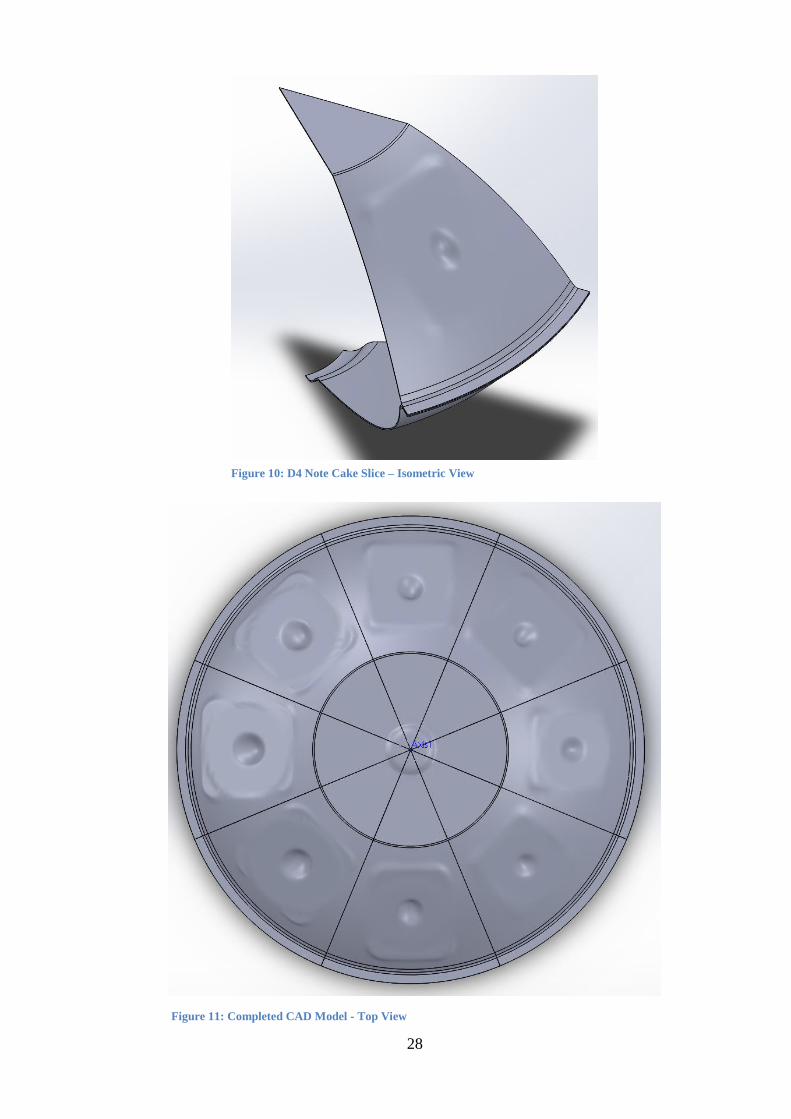
4.3 Outcomes
An example of a single slice note is shown in Figure 10. Between notes only the panel section
of the notes changes but as they all have similar features, this note is customisable in its key
geometries. An example of the completed assembly is shown in Figure 11. This compares very
well to the actual instrument in Figure 9.
Figure 9: Cake Slice View
28
Figure 10: D4 Note Cake Slice – Isometric View
Figure 11: Completed CAD Model - Top View

29
4.4 Further Work
4.4.1 3D Scan
While a data point field is not suitable for the purpose of analysis it does have value if it is
available. This is available at UQ, however, the author was not aware until late in the thesis so
work utilising this tool is rudimentary. Figure 12 shows the data point field scan of the Pi Drum
instrument. This scan is particularly useful for drawing out geometric information to feed into
the existing model.
It is also possible to compare CAD models to this data point field to examine their fidelity in
modelling geometry. This was not performed as there was insufficient time, however, it would
be a very useful tool for CAD model validation and verification.
Figure 12: 3D Scan - Pi Drum

30
4.4.2 Other Instruments
Cake slice methods are not as useful when the geometry is not symmetric and equal sized slices
cannot be used. However, it can still be useful in the modelling. Slices are no longer able to be
equal in size and as reusable. Slices of different sizes need to be used and the methods of
creating deformation remain the same but are more time consuming. This is applicable to many
handpans, including the further studied Meridian handpan in Figure 13.
4.5 Discussion and Recommendations
Current methodology provides a robust and customisable CAD model. Using 3D scans to create
geometrically more accurate and precise models will increase model performance and provide
better FE study results. Clearly, the existing CAD model is a good representation of the Pi Drum
but 3D scans show that improvement can be made.
Moving forward, the 3D scan should be used to improve existing CAD models. Analytical
results show that modal frequency is highly sensitive to geometry. Therefore, increased model
accuracy may provide the largest increase in correlation between physical and digital results.
Figure 13: Meridian Handpan
31
5 THEORETICAL ANALYSIS
5.1 Introduction
Existing analytical plate vibrations theory as presented in 2.1.6 can be used to provide estimates
of modal frequencies. All that is required is material properties, assumptions of vibrational
mode, and measurements of the physical system. These equations will also provide insight into
how certain geometric variables will change modal frequencies.
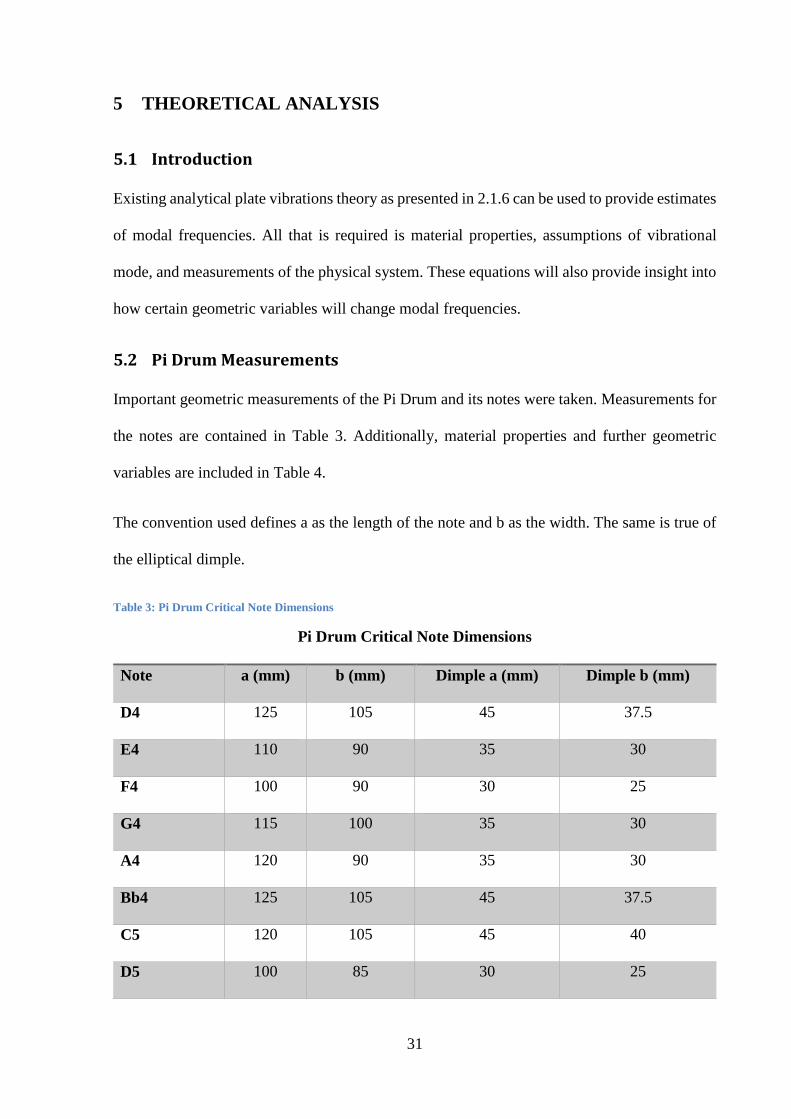
5.2 Pi Drum Measurements
Important geometric measurements of the Pi Drum and its notes were taken. Measurements for
the notes are contained in Table 3. Additionally, material properties and further geometric
variables are included in Table 4.
The convention used defines a as the length of the note and b as the width. The same is true of
the elliptical dimple.
Table 3: Pi Drum Critical Note Dimensions
Pi Drum Critical Note Dimensions
Note a (mm) b (mm) Dimple a (mm) Dimple b (mm)
D4 125 105 45 37.5
E4 110 90 35 30
F4 100 90 30 25
G4 115 100 35 30
A4 120 90 35 30
Bb4 125 105 45 37.5
C5 120 105 45 40
D5 100 85 30 25

32
Table 4: Pi Drum Variables
Pi Drum Variables
Variable Name Value Units
E Elastic Modulus 207 GPa
ν Poisson's Ratio 0.3 Unitless
h Plate thickness 0.95 mm
ρ Density 7800
𝑘𝑔
𝑚3
Plate thickness was determined by finding the surface area of the CAD model and dividing the
mass of the Pi Drum by this figure.
5.2.1 Rectangular Plates
Using 2.1.6.1 and the information in Table 3 and Table 4 estimates of the modal frequencies of
the notes can be made by assuming they are rectangular plates and the dimples are not present.
This was done for two boundary conditions; all edges simply supported (SS) and all edges fixed
(often called clamped). Table 5 contains the results for the actual thickness plate, double
thickness plate and the measured value of the fundamental mode from section 3.4. The plot of
the data for actual thickness and measured data is shown in Figure 14. All results are in Hz.
Table 5: Analytical Solutions - Rectangular Plate
Pi Drum Analytical Solutions – Rectangular Plate
Note Measured SS Fixed SS Double Fixed Double
D4 294.3 359.9 630.5 719.8 1260.9
E4 333 479.5 829.4 958.9 1658.9
F4 351.7 519.8 939.4 1039.7 1878.8
G4 393.2 408.5 727.2 817.1 1454.3

33
A4 442.4 448.8 742.7 897.5 1485.4
Bb4 467.4 359.9 630.5 719.8 1260.9
C5 524.8 372.6 665.0 745.1 1330.0
D5 589 554.6 977.0 1109.2 1953.9
5.2.2 Circular Plates
Estimates of the modal frequencies of the notes can be made by assuming they are circular
plates and the dimples are not present. The width of the plate was taken as the diameter of the
plate. This was done for two boundary conditions; edge is simply supported (SS) and edge is
fixed. Table 6 contains the results for the actual and double thickness plate. The plot of the
actual thickness and measured data is shown in Figure 15. All results are in Hz.
Table 6: Analytical Solutions - Circular Plate
Pi Drum Analytical Solutions – Circular Plate
Note Measured SS Fixed SS Double Fixed Double
D4 294.3 425.6 873.6 851.2 1747.3
E4 333 579.3 1189.1 1158.6 2378.2
200
300
400
500
600
700
800
900
1000
D4 E4 F4 G4 A4 Bb4 C5 D5
Freq
uen
cy (
Hz)
Rectangular Plate Theory
Measured
SS
Fixed
Figure 14: Rectangular Plate Results - Line Graph

34
F4 351.7 579.3 1189.1 1158.6 2378.2
G4 393.2 469.2 963.2 938.5 1926.4
A4 442.4 579.3 1189.1 1158.6 2378.2
Bb4 467.4 425.6 873.6 851.2 1747.3
C5 524.8 425.6 873.6 851.2 1747.3
D5 589 649.5 1333.1 1298.9 2666.3
5.2.3 Annular Plates
Estimates of the modal frequencies of the notes can be made by assuming they are annular
plates and the dimples are a cut out in the middle of the plate. The dimensions of the annular
ring are taken as the average of the dimple a and b dimensions as inner diameter and the width
of the plate as the outer diameter. This was done for two boundary conditions; both edges
simply supported (SS) and both edges fixed (CC). Table 7 contains the results for the actual
and double thickness plate. The plot of the actual thickness and measured data is shown in
Figure 16. All results are in Hz.
0.0
200.0
400.0
600.0
800.0
1000.0
1200.0
1400.0
D4 E4 F4 G4 A4 Bb4 C5 D5
Freq
uen
cy (
Hz)
Circular Plate Theory
SS
CC
Actual Note
Figure 15: Circular Plate Results

35
Table 7: Analytical Solutions - Annular Plate
Pi Drum Analytical Solutions – Annular Plate
Note Measured SS CC SS Double CC Double
D4 294.3 536.7 1178.2 1073.4 2356.3
E4 333 685.9 1475.9 1371.9 2951.9
F4 351.7 594.7 1219.9 1189.4 2439.8
G4 393.2 509.5 1065.4 1019.1 2130.8
A4 442.4 685.9 1475.9 1371.9 2951.9
Bb4 467.4 536.7 1178.2 1073.4 2356.3
C5 524.8 571.9 1279.9 1143.8 2559.7
D5 589 694.7 1445.2 1389.4 2890.5
5.3 Discussion
Theoretical results do not seem to provide a good match to actual notes. This can be seen by
that fact that all annular plate results are above the actual note as are almost all circular and
rectangular results (Figure 14, Figure 15 and Figure 16). Assuming these theoretical results
0.0
200.0
400.0
600.0
800.0
1000.0
1200.0
1400.0
1600.0
D4 E4 F4 G4 A4 Bb4 C5 D5
Freq
uen
cy (
Hz)
Annular Plate Theory
SS
CC
Actual Note
Figure 16: Annular Plate Results

36
should be close to the actual note it informs that the simply supported case is always much
closer to reality than the fixed case. This is unsurprising as the real note is supported by a
membrane of material.
Circular plate theory seems to provide the closest results to real life. If the circular mode shapes
shown in Figure 8 are those of real notes, then circular plate theory would provide a mode shape
closest to this. This is an interesting point of how the note behaves and warrants further
investigation via FEA.
Interestingly, doubling the thickness of a note doubles the frequency of that note. This is a linear
relationship, not cubic as it would seem from the equations. Thickness is still, however, a major
driver of frequency. The thickness estimate made at the start of this section and used in
calculations may not be reliable. It relies on top and bottom shell being equally thick and used
a rough measurement of mass. Using geometric data from the 3D scan and mass method may
improve the estimate with potential direct measurement methods being preferable. Improved
thickness measurements may provide major return in model accuracy.
Importantly, it is the opinion of the author that the dimple in the centre of the note has a strong
impact on the note response that is not easily quantifiable nor its change qualitatively simple.
This is suspected because notes of almost identical dimensions such as D4 and Bb4 have
different notes but their dimple is different in depth. Furthermore, the way in which the note
panel is made into the shell of the instrument may affect the boundary conditions. If a note is
raised with material perpendicular to the surface of the shell at the edge of the note, this may
make the boundary condition shift to a stiffer boundary condition, having a large effect.

37
6 FEA ANALYSIS
6.1 Introduction
Finite Element Analysis was performed on both the full assembly of the instrument and
individual notes. The results of individual notes are much more informative about what is
actually occurring in the areas of interest. Previous research has shown that analysis of
individual notes is a valid methodology as interactions are not dominant. Modal analysis solves
the Eigen equation to find mode shapes and frequencies. Transient analysis solves the complete
set of FE equations at each time step and updates values accordingly, such as stiffness matrix
based on geometric changes. Both methods are utilised. In both cases solid shell elements were
utilised.
6.2 Modal Analysis
6.2.1 Method and Set-Up
To run a simulation follow the steps outlined. For a complete methodology refer to Appendix .
1. Import geometry into ANSYS as a .STEP file and suppress the die used to create the
note indentation.
2. In Workbench Mechanical Set the Model and Modal parameters as described in
Appendix D. Primarily focus on correct contact region, mesh method, supports and
analysis settings.
3. Run the solver and view the results.
6.2.2 Results
Modal analysis produces results files such as that shown in Figure 17. It is useful because the
mode shape and corresponding modal frequency can be viewed. Table 8 contains the first modal
frequency for all notes in Hz and the measured frequency from the actual Pi Drum handpan.

38
Table 8: Modal Analysis Frequencies
Pi Drum FEA – Modal Results
Note Modal Measured
D4 617.9 294.3
E4 654.9 333
F4 776.7 351.7
G4 661.1 393.2
A4 781.2 442.4
Bb4 615.6 467.4
Figure 17: Example Modal Result

39
C5 627.6 524.8
D5 784.2 589
6.3 Transient Analysis
6.3.1 Method and Set Up
Transient analyses do not provide results in the same manner as modal. It is not possible to
directly draw a frequency from the program. Thus a time history for a node or group of nodes
needs to be extracted from the target note and then passed through an FFT. While the overall
setup in ANSYS is almost identical there are some extra steps outlined in Appendix D.
Some key points regarding the analysis are:
1. A time step in the analysis of 2.5*10-5 seconds,
2. A total number of time increments of 2048 (211),
3. A triangular impulse peaking at 20N applied over 40 time steps (0.001 seconds),
4. Load applied just above the dimple on each note,
5. Time history taken on a node just below the dimple on each note.
6.3.2 Results
Excel was used to analyse the time series data of a node on the desired note. Figure 18 shows
the FFT of the A4 note performed in excel. Table 9 contains the data for all notes transient and
modal analysis as well as measured note frequency. Figure 19 shows these data graphically.
Appendix D (Figure 80 to Figure 87) shows the FFT for all notes presented.

40
Table 9: Transient, Modal and Measured Frequencies
Pi Drum FEA – Transient Results
Note Transient Measured Modal
D4 312.5 294.3 617.9
E4 293 333 654.9
F4 390 351.7 776.7
G4 507 393.2 661.1
A4 469 442.4 781.2
Bb4 449 467.4 615.6
C5 469 524.8 627.6
D5 586 589 784.2
0
1
2
3
4
5
6
100.00 200.00 300.00 400.00 500.00 600.00 700.00
FFT
Co
mp
on
ent
Frequency (Hz)
FFT Transient - Bb4 Note
Figure 18: FFT of A4 Note

41
6.4 Discussion
Transient analysis of the notes provides a great increase in result quality when compared to the
actual instrument. This suggests that non-linear effects need to be taken into account to get
accurate results. While they are a significant improvement over modal they still leave a large
amount to be desired.
Interestingly, the modal results show little fluctuation for all notes. Importantly the mode shape
acquired from the modal analysis aligns with what is expected from previous work on hanpdans.
It seems to behave as an almost circular plate in its shape. This is a good indicator that the
model has validity.
The author is unsure if the transient results provide sufficient accuracy. Perhaps geometric
effects are so significant that current geometry is not accurate enough. This is likely a leading
cause of the discrepancy between transient and physical results.
250
350
450
550
650
750
850
D4 E4 F4 G4 A4 Bb4 C5 D5
Freq
uen
cy (
Hz)
Note
Actual Note vs Modal and Transient Analysis Fundamental Frequencies
Measured
Modal
Transient
Figure 19: Transient, Modal and Measured Results Line Graph

42
7 GEOMETRIC EFFECTS
7.1 Introduction
Note D5 on the Pi Drum shows the greatest correlation between the FEA model and physical
instrument. As such, this note will be used to investigate geometric effects on modal response.
Some simple geometric changes are used including: doubling the thickness of the material,
removing the dimple, raising the note up so it has stiffer edges and altering the aspect ratio of
the note. These effects should provide a baseline for what effects are most significant.
7.2 Method
A CAD model of the D5 note was modified to have the following geometric changes:
No Dimple,
Double plate thickness,
A raised note,
Double the aspect ratio (AR) with and without a dimple,
Half the AR with and without a dimple and,
Normal note dimensions.
These geometric changes were then analysed via modal and transient analysis respectively.
For all notes the effect of removing the dimple, doubling the thickness and raising the note was
analysed via modal analysis. For consistency these were only compared with other modal
results and the more detailed analysis of the D5 note was compared within itself.
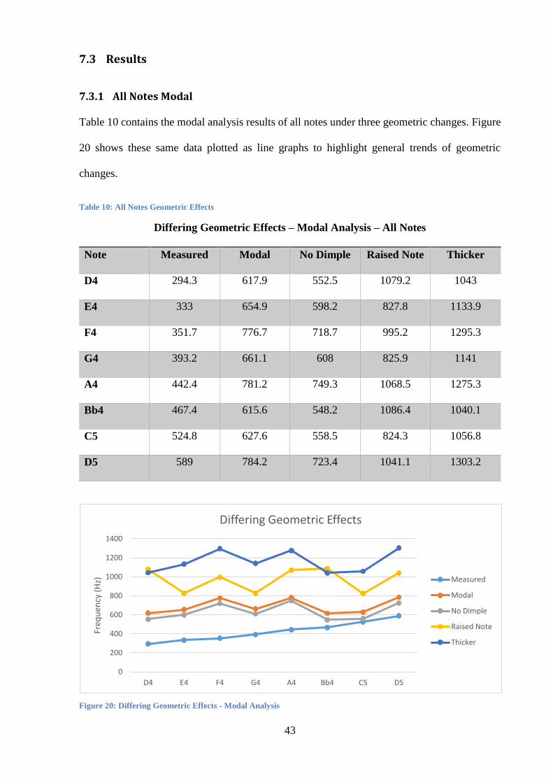
43
7.3 Results
7.3.1 All Notes Modal
Table 10 contains the modal analysis results of all notes under three geometric changes. Figure
20 shows these same data plotted as line graphs to highlight general trends of geometric
changes.
Table 10: All Notes Geometric Effects
Differing Geometric Effects – Modal Analysis – All Notes
Note Measured Modal No Dimple Raised Note Thicker
D4 294.3 617.9 552.5 1079.2 1043
E4 333 654.9 598.2 827.8 1133.9
F4 351.7 776.7 718.7 995.2 1295.3
G4 393.2 661.1 608 825.9 1141
A4 442.4 781.2 749.3 1068.5 1275.3
Bb4 467.4 615.6 548.2 1086.4 1040.1
C5 524.8 627.6 558.5 824.3 1056.8
D5 589 784.2 723.4 1041.1 1303.2
0
200
400
600
800
1000
1200
1400
D4 E4 F4 G4 A4 Bb4 C5 D5
Freq
uen
cy (
Hz)
Differing Geometric Effects
Measured
Modal
No Dimple
Raised Note
Thicker
Figure 20: Differing Geometric Effects - Modal Analysis

44
7.3.2 D5 Note Analysis
All geometric effects were analysed for the D5 note and the data for modal and transient
analyses are presented in Table 11 and Figure 21, with FFTs of notes in Appendix E.
Table 11: D5 Note - Modal and Transient Analysis
D5 Note Modal and Transient Analysis
Type Modal Transient
No Dimple 552.5 527.3
Measured 589 589
Normal 617.9 586
Double Thickness 1043 937.5
Raised 1079.2 918
Double AR No Dimple 1295.1 1015.6
Double AR 1457.2 1035.2
Half AR 1920.7 1035.2
Half AR No Dimple 2390.7 1113.3
0
500
1000
1500
2000
2500
Freq
uen
cy (
Hz)
Modal vs Transient Geometric Effects - D5 Note
Modal
Transient
Figure 21: D5 Note - Modal vs Transient Geometric Effects

45
7.4 Discussion
Geometric changes have been studied in a broad but shallow manner. Changes examined can
provide an idea of general trends for certain changes but no detailed insight. Figure 20 provides
useful trend comparison for each change studied. Removing the dimple has a measurable and
significant change of a 50 Hz reduction in modal frequency compared to the normal note. It
follows the same trend pattern too. Very interestingly doubling the thickness of the note does
not quite double the modal frequency.
Raising the note to make the boundary condition stiffer has an erratic effect on modal frequency
but always increases it by a minimum of 30%. This erratic change is too be expected as differing
sized notes have differing amounts of raised material leading into the note and thus varying
stiffness’s along the edges of the notes.
In all modal analyses the FEA result is above the actual note of the instrument. In some cases
it is by only a small amount (C5 note) and in others it is decided pronounced (F4 note). This is
an interesting point and warrants further investigation.
Modal and transient analyses provide a point of further interest. In all examined notes the
transient analysis shows a lower frequency that the modal. This was expected but it becomes
particularly pronounced at the effects that create higher frequencies. Differences between modal
and transient results are limited for the normal note but a twofold difference is present in the
Half AR notes. This is another interesting point and warrants further investigation.

46
8 DISCUSSION
Physical testing was a less rigorous process than had been envisaged. Using a human finger
without a standardised strike imparts some uncertainty into the results. However, the alternative
of using a striker produced high pitched responses and in reality a human finger is used while
playing the instrument. Also, using the anechoic chamber created sharper results than would be
otherwise attainable. Results show very low levels of error compared to expected notes with
both the Pi Drum and Meridian which indicates the method is not fundamentally flawed,
assuming the instruments were well tuned to begin with. Thus, baseline testing resulting can be
deemed both precise and accurate. Some key differences between the instruments provide much
insight into possible further investigation.
Existing CAD modelling procedures are both expandable to other instruments and useful for
examining geometric changes. However, as shown by Figure 12 there is a method for achieving
greater accuracy and precision. The organic nature of the shapes in these instruments makes the
CAD modelling process the most challenging part of any project with these instruments.
Balancing a customisable model and exactness of geometry is a headwind to progress. Using
an augmented 3D scan information and current modelling techniques method will result in
superior models.
Theoretical analysis provides a baseline for expected frequencies but seems to be vastly
different from measured modal frequencies. One possible source of some of this error is
imprecision in measurements taken of the geometry. Primarily, the thickness calculation, which
strongly influences theoretical analysis, was a simple calculation. The method of weighing and
finding surface to calculate thickness may not be sufficiently accurate. Furthermore, the
equations used are highly sensitive to geometry (including thickness) and boundary conditions.
Estimating the boundary conditions therefore has a large effect. Following this, the organic

47
nature of geometry means measurement errors will be significant and this can also have a large
impact on the theoretical results.
Based on Figure 7 and Figure 8 it can be assumed that circular plate type modal vibrations are
occurring in the note region of the instrument. This aligns with circular plate theory providing
the closest correlation between theory and practicality. Further FEA confirmed that the plate
seemed to be vibrating in an almost circular mode as shown in Figure 17. The modal values
attained from FEA followed the trend of theoretical calculations in being far above physically
observed frequencies. This suggests that non-linearities in the system are significant, geometric
sensitivities are very high or both.
Transient analyses provided more realistic results when compared to modal but where still often
significantly different from observed results. Again, sensitivity to geometry likely had an effect.
Some notes aligned transient and reality quite well, such as the D5 note. This could be due to
chance that its geometry was better aligned but more likely attributable to chance.
Dimples in the centre of the note provide an interesting phenomena. They lower the observed
frequency in both transient and modal analyses. Reasons for this drop could be it affecting
boundary conditions or making the plate behave with greater stiffness in the middle. The drop
in frequency the dimples cause is consistent across all notes analysed.
Raising the note creates a stiffer edge, approximating a more fixed edge condition. This, as
expected, increased the frequency of the note. Because of the inconsistent nature of raising the
edges (different sized notes have different amounts of raised edge, for example) the change
caused is also inconsistent. Figure 20 shows this is in contrast with other simple geometric
changes, which still follow the same profile between notes at different frequencies.
48
9 CONCLUSIONS AND RECOMMENDATIONS
9.1 Conclusions
While a specific, highly repeatable, method for physical testing of handpans was not developed,
the method generated and used provided consistent and realistic results. True scientific
repeatability was not achieved for the method but error minimisation was still realized and the
use of an anechoic chamber and high fidelity microphone gave clean, consistent data. Further
experimentation on the instruments need not deviate from existing methods, if it is required at
all.
Physical testing provided a confirmation of the interaction between notes the instrument
experiences. However, it also showed that these interactions do not affect model frequencies.
Furthermore, comparing results from both instruments highlighted the increased damping
present in the Pi Drum. This damping was likely caused by two things; the joint of the two
shells and structural damping within the steel. This is a candidate for further investigation and
increased modelling attention.
CAD modelling procedures were developed entirely from scratch for this project. Existing
methodology is very useful for its customisable nature but could be improved by augmenting it
with accurate 3D scan information. Current models are not accurate enough to capture the
geometry sufficiently and need to be improved for results that correlate more precisely with
physical systems. This may be the single largest improvement that can be made to the digital
modelling process.
Theoretical analysis of the notes provided interesting insight into the behaviour of the system.
Thickness calculations were not particularly robust and may have had a significant impact on
results attained. In combination with the mode shapes from FEA the analytical results suggest
the notes vibrate in a circular plate manner. This is a point of interest and may be informative

49
for further work. This analysis showed that the frequencies present are highly dependent on and
sensitive too geometry. Using more accurate geometric information from the 3D scan may help
improve the correlation between theoretical and physical results.
Modal frequencies attained from FEA analysis of the notes suggest that non-linearities are
significant. This is in agreement with existing literature too. Overall trends of modal analysis
provided some insight into system behaviour but did not provide predictive capability as the
results were far off physical outcomes, in some cases by over 200%. Transient analysis showed
that non-linear solving of the system provided much more accurate results but still had large
improvements to be made. Thus, non-linearities are a driving factor and need to be considered.
All geometric changes when analysed via modal and transient had the same trend movement
and followed what would be expected. This is good for model validation purposes and helped
provide insight into what can affect the note present. Particularly the raised edge notes had large
increases in frequency and this may be a useful method of controlling frequencies present, along
with the dimple.
A superficial examination of geometric effects of the handpan is presented in this dissertation.
Once modelling methods and models are improved a far deeper exploration of geometric effects
should be undertaken. This investigation is a thesis in its own right.
9.2 Recommendations
Recommendations for further or improved work follow:
CAD model accuracy improvements. This should be done using the existing models and
improved data from the 3D scan. Particularly, note die geometry in the SolidWorks
model can be greatly improved and thus provide a closer representation to real life. The
dimple, which is suspected to have a significant effect, can also be improved using this
enhanced geometric data.

50
Improve the thickness estimate by measuring directly if possible. Otherwise, use 3D
scan information and a more accurate mass measurement to improve the result. It may
be the case that top and bottom halves of the instrument are not of equal thickness.
With improved geometry perform modal analysis on individual notes once again and
observe the amount of improvement in results. Also, run a full instrument model FEA
and observe for fundamental frequencies there. This process may be highly informative.
Perform theoretical analysis of notes once again with improved geometric information.
Once again, this may be highly informative as improved inputs may show that
theoretical analysis, in some form, is useful for design purposes.
With improved models, examine geometric changes in greater detail. For example, do
not only look at two changes in AR, make a refined grid so the response to AR can be
plotted for a note. Examine differing dimple geometries, not just their removal.
Improve the modelling of damping in the system when performing FEA. Focus
especially on the rim joint of the two shells.
Create a CAD model of the Meridian handpan and analyse this. Its slightly more
consistent geometry and reduced damping may mean it is more conducive to modelling
and provide greater insight (i.e. less noise in the analysis to worry about).
Further direction for investigation will be found when performing these recommendations.
51
10 REFERENCES
Achong, A. (1996). "The steelpan as a system of non-linear mode-localized oscillators, I:
Theory, simulations, experiments and bifurcations." Journal of Sound and Vibration 197(4):
471-487.
Achong, A. (1996). "Vibrational analysis of mass loaded plates and shallow shells by the
receptance method with application to the steelpan." Journal of sound and vibration 191(2):
207-217.
Achong, A. and K. Sinanan-Singh (1997). "The steelpan as a system of non-linear mode-
localized oscillators, part II: coupled sub-systems, simulations and experiments." Journal of
sound and vibration 203(4): 547-561.
Adams, V. and A. Askenazi (1999). Building Better Products with Finite Element Analysis,
OnWord Press.
Alon, E. (2015). Analysis and Synthesis of the Handpan Sound, University of York.
Alon, E. and D. T. Murphy (2015). "ANALYSIS AND RESYNTHESIS OF THE HANDPAN
SOUND."
Gay, D. A. (2008). "Finite element modelling of steelpan acoustics." Journal of the Acoustical
Society of America 123(5): 3799-3799.
Google (2017). Handpan Manufacturers. Mountain View, Google.

52
Han, W. and M. Petyt (1997). "Geometrically nonlinear vibration analysis of thin, rectangular
plates using the hierarchical finite element method—I: The fundamental mode of isotropic
plates." Computers & Structures 63(2): 295-308.
ICT, N. (2017). "Free Vibration of a Cantilever Beam (Continuous System)." Retrieved 9th of
September, 2017, from http://iitg.vlab.co.in/?sub=62&brch=175&sim=1080&cnt=1.
Leissa, A. W. (1969). Vibration of plates, OHIO STATE UNIV COLUMBUS.
Leissa, A. W. (1973). "The free vibration of rectangular plates." Journal of Sound and Vibration
31(3): 257-293.
Monteil, M., C. Touzé and O. Thomas (2013). "Nonlinear vibrations of steelpans: analysis of
mode coupling in view of modal sound synthesis."
Morrison, A. and T. Rossing (2007). "Modes of vibration and sound radiation from the hang."
Archives of Acoustics 32(3): 551-560.
Paniverse. (2017). "DEEPAN in progress – New generation Pan’s." Retrieved 20th of October,
2017, from https://i1.wp.com/paniverse.org/wp-content/uploads/2016/06/20160618_165758-
e1466491305592.jpg.
Rao, S. S. (2011). Mechanical vibrations, Prentice Hall Upper Saddle River.
53
Rohner, F. and S. Schärer (2007). History, Development and Tuning of the HANG.
International Symposium on Musical Acoustics (ISMA 2007).
Rossing, T., A. Morrison, U. Hansen, F. Rohner and S. Schärer (2007). Acoustics of the Hang:
A hand-played steel instrument. International Symposium on Musical Acoustics (ISMA 2007).
Shi, D., X. Shi, W. L. Li, Q. Wang and J. Han (2014). "Vibration Analysis of Annular Sector
Plates under Different Boundary Conditions." Shock and Vibration 2014: 11.
Software, M. (2011). Dynamic Analysis User's Guide: MSC Nastran 2012, MacNeal-
Schwendler Corporation.

54
11 APPENDICES
11.1 Appendix A
11.1.1 Analytical Rectangular Plate Solution Coefficients
Figure 22: Rectangular Plate Boundary Condition Constants
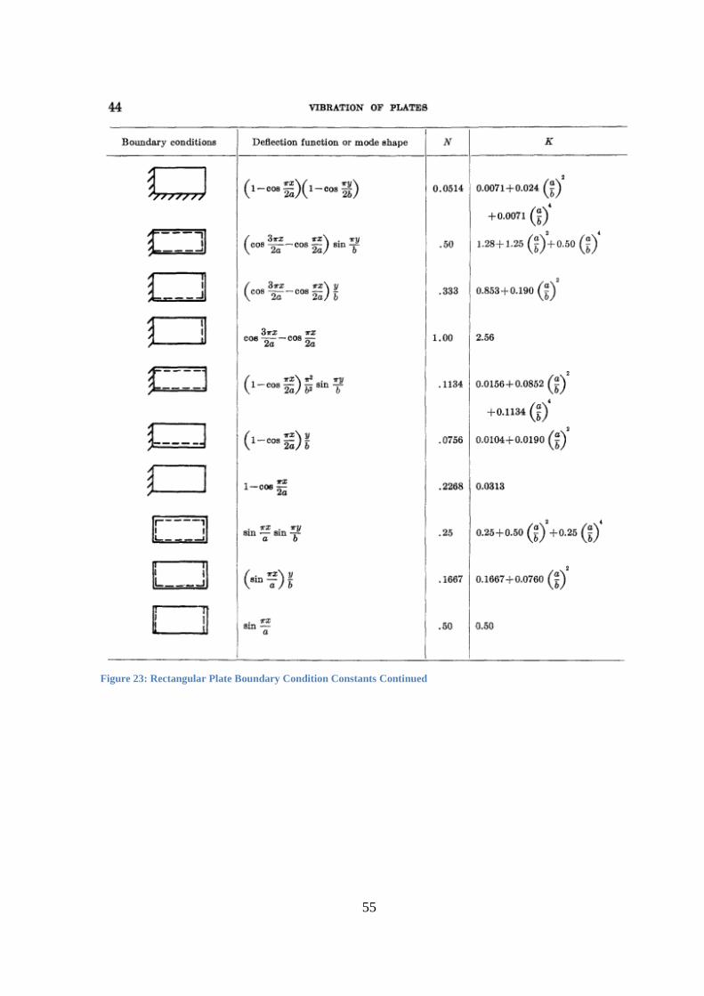
55
Figure 23: Rectangular Plate Boundary Condition Constants Continued

56
11.1.2 Analytical Circular Plate Solution Coefficients
Figure 24: Clamped Circular Plate Boundary Condition Constants
Figure 25: Simply Supported Circular Plate Boundary Condition Constants
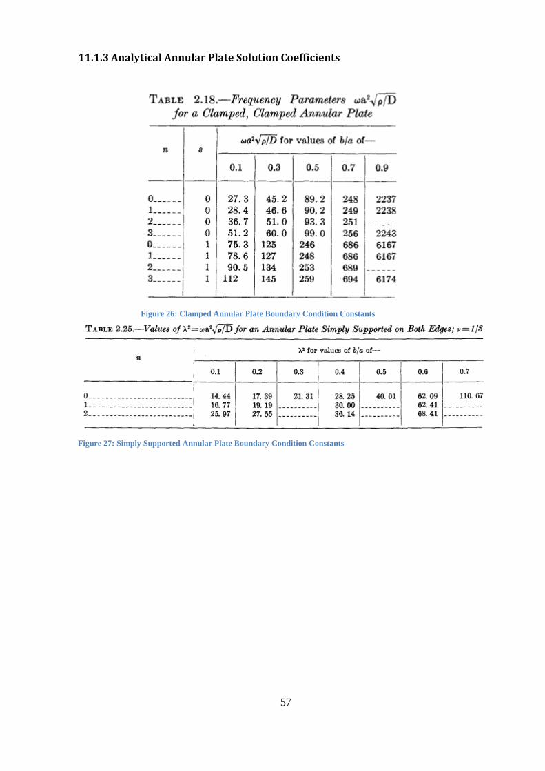
57
11.1.3 Analytical Annular Plate Solution Coefficients
Figure 26: Clamped Annular Plate Boundary Condition Constants
Figure 27: Simply Supported Annular Plate Boundary Condition Constants

58
11.2 Appendix B
11.2.1 Matlab Code for Audio Sample Analysis
Figure 28: Audio Sample Analysis Matlab Code
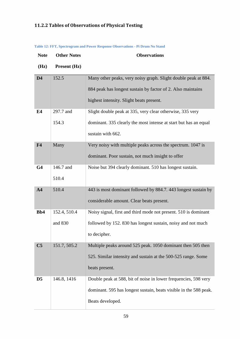
59
11.2.2 Tables of Observations of Physical Testing
Table 12: FFT, Spectrogram and Power Response Observations - Pi Drum No Stand
Note
(Hz)
Other Notes
Present (Hz)
Observations
D4 152.5 Many other peaks, very noisy graph. Slight double peak at 884.
884 peak has longest sustain by factor of 2. Also maintains
highest intensity. Slight beats present.
E4 297.7 and
154.3
Slight double peak at 335, very clear otherwise, 335 very
dominant. 335 clearly the most intense at start but has an equal
sustain with 662.
F4 Many Very noisy with multiple peaks across the spectrum. 1047 is
dominant. Poor sustain, not much insight to offer
G4 146.7 and
510.4
Noise but 394 clearly dominant. 510 has longest sustain.
A4 510.4 443 is most dominant followed by 884.7. 443 longest sustain by
considerable amount. Clear beats present.
Bb4 152.4, 510.4
and 830
Noisy signal, first and third mode not present. 510 is dominant
followed by 152. 830 has longest sustain, noisy and not much
to decipher.
C5 151.7, 505.2 Multiple peaks around 525 peak. 1050 dominant then 505 then
525. Similar intensity and sustain at the 500-525 range. Some
beats present.
D5 146.8, 1416 Double peak at 588, bit of noise in lower frequencies, 598 very
dominant. 595 has longest sustain, beats visible in the 588 peak.
Beats developed.
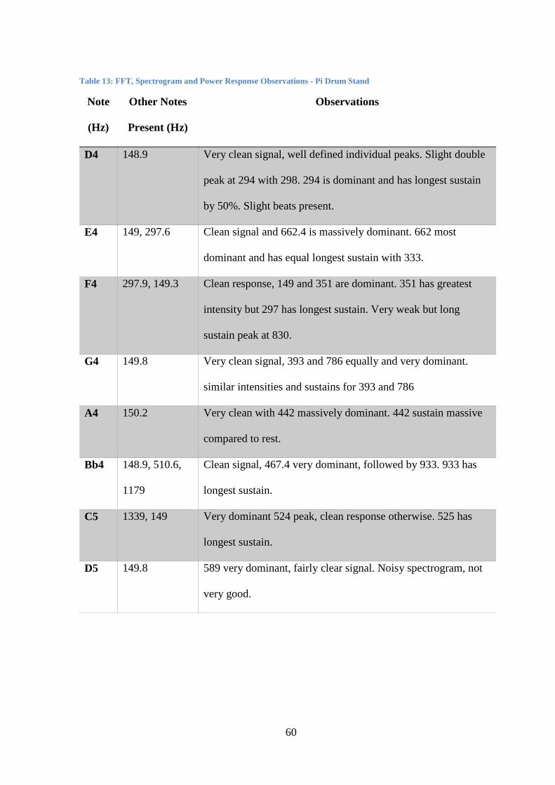
60
Table 13: FFT, Spectrogram and Power Response Observations - Pi Drum Stand
Note
(Hz)
Other Notes
Present (Hz)
Observations
D4 148.9 Very clean signal, well defined individual peaks. Slight double
peak at 294 with 298. 294 is dominant and has longest sustain
by 50%. Slight beats present.
E4 149, 297.6 Clean signal and 662.4 is massively dominant. 662 most
dominant and has equal longest sustain with 333.
F4 297.9, 149.3 Clean response, 149 and 351 are dominant. 351 has greatest
intensity but 297 has longest sustain. Very weak but long
sustain peak at 830.
G4 149.8 Very clean signal, 393 and 786 equally and very dominant.
similar intensities and sustains for 393 and 786
A4 150.2 Very clean with 442 massively dominant. 442 sustain massive
compared to rest.
Bb4 148.9, 510.6,
1179
Clean signal, 467.4 very dominant, followed by 933. 933 has
longest sustain.
C5 1339, 149 Very dominant 524 peak, clean response otherwise. 525 has
longest sustain.
D5 149.8 589 very dominant, fairly clear signal. Noisy spectrogram, not
very good.
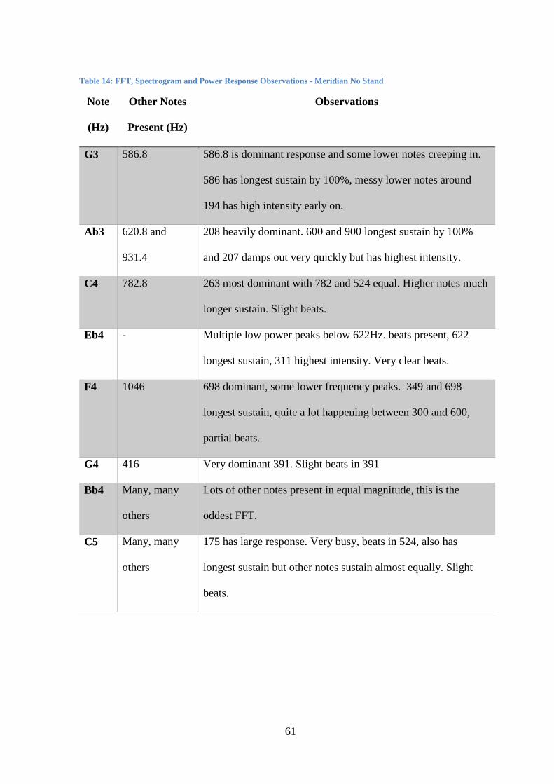
61
Table 14: FFT, Spectrogram and Power Response Observations - Meridian No Stand
Note
(Hz)
Other Notes
Present (Hz)
Observations
G3 586.8 586.8 is dominant response and some lower notes creeping in.
586 has longest sustain by 100%, messy lower notes around
194 has high intensity early on.
Ab3 620.8 and
931.4
208 heavily dominant. 600 and 900 longest sustain by 100%
and 207 damps out very quickly but has highest intensity.
C4 782.8 263 most dominant with 782 and 524 equal. Higher notes much
longer sustain. Slight beats.
Eb4 - Multiple low power peaks below 622Hz. beats present, 622
longest sustain, 311 highest intensity. Very clear beats.
F4 1046 698 dominant, some lower frequency peaks. 349 and 698
longest sustain, quite a lot happening between 300 and 600,
partial beats.
G4 416 Very dominant 391. Slight beats in 391
Bb4 Many, many
others
Lots of other notes present in equal magnitude, this is the
oddest FFT.
C5 Many, many
others
175 has large response. Very busy, beats in 524, also has
longest sustain but other notes sustain almost equally. Slight
beats.

62
Table 15: FFT, Spectrogram and Power Response Observations - Meridian Stand
Note
(Hz)
Other Notes
Present (Hz)
Observations
G3 586.6 586 is equal magnitude to 195.4. 586 has longest sustain by
100%, large amount of notes between 195 and 586. Nice decay
Ab3 620.7 620 is close to e flat 5. 620 has longest sustain by 30% but 207
has highest intensity. Slight beats.
C4 782.8 Linear decrease in power from 262 to 1046. Longest sustain on
700 but 500 700 and 1000 all roughly equal. Messy minor
beats.
Eb4 - Some other low power notes present. 622 has longest sustain.
310 highest intensity. Slight development of beats.
F4 - Some low power lower frequency notes. 698 is highest intensity
and longest sustain, beats in 350. Clear beats.
G4 415 783 dominant followed by 390.8. 783 has highest in intensity
and longest sustain.
Bb4 Many others Again, many other notes present. Beats in 350, 1045 longest,
very busy spectrogram.
C5 Multiple others
present
Very busy FFT. Beats in 520, also has longest sustain, very
busy and cramped.

63
11.2.3 Pi Drum Spectrograms
11.2.3.1 D4
Figure 30: Pi Drum - D4 Spectrogram - Stand
Figure 29: Pi Drum - D4 Spectrogram – No Stand

64
11.2.3.2 E4
Figure 31: Pi Drum - E4 Spectrogram – No Stand
Figure 32: Pi Drum - E4 Spectrogram – Stand
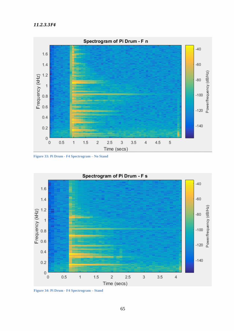
65
11.2.3.3 F4
Figure 33: Pi Drum - F4 Spectrogram – No Stand
Figure 34: Pi Drum - F4 Spectrogram – Stand

66
11.2.3.4 G4
Figure 35: Pi Drum - G4 Spectrogram – No Stand
Figure 36: Pi Drum - G4 Spectrogram – Stand
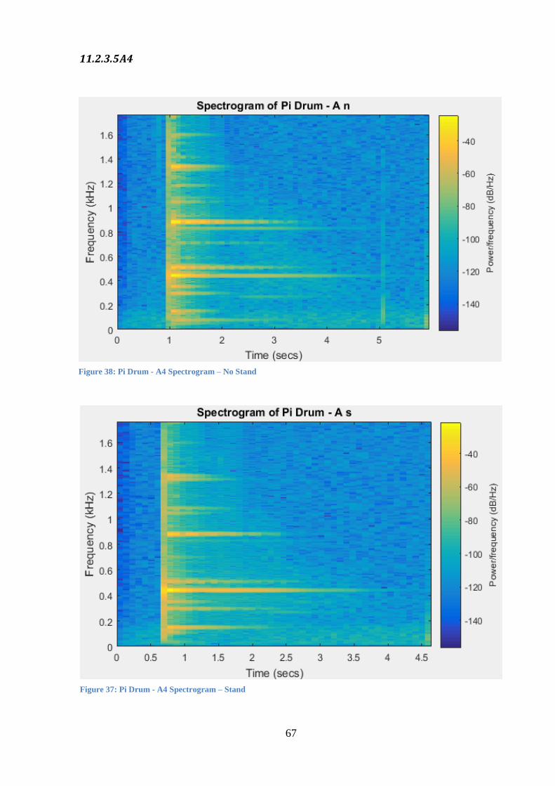
67
11.2.3.5 A4
Figure 38: Pi Drum - A4 Spectrogram – No Stand
Figure 37: Pi Drum - A4 Spectrogram – Stand

68
11.2.3.6 Bb4
Figure 40: Pi Drum - Bb4 Spectrogram – No Stand
Figure 39: Pi Drum - Bb4 Spectrogram – Stand
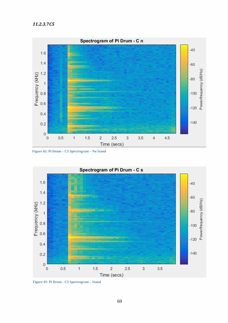
69
11.2.3.7 C5
Figure 42: Pi Drum – C5 Spectrogram – No Stand
Figure 41: Pi Drum - C5 Spectrogram – Stand
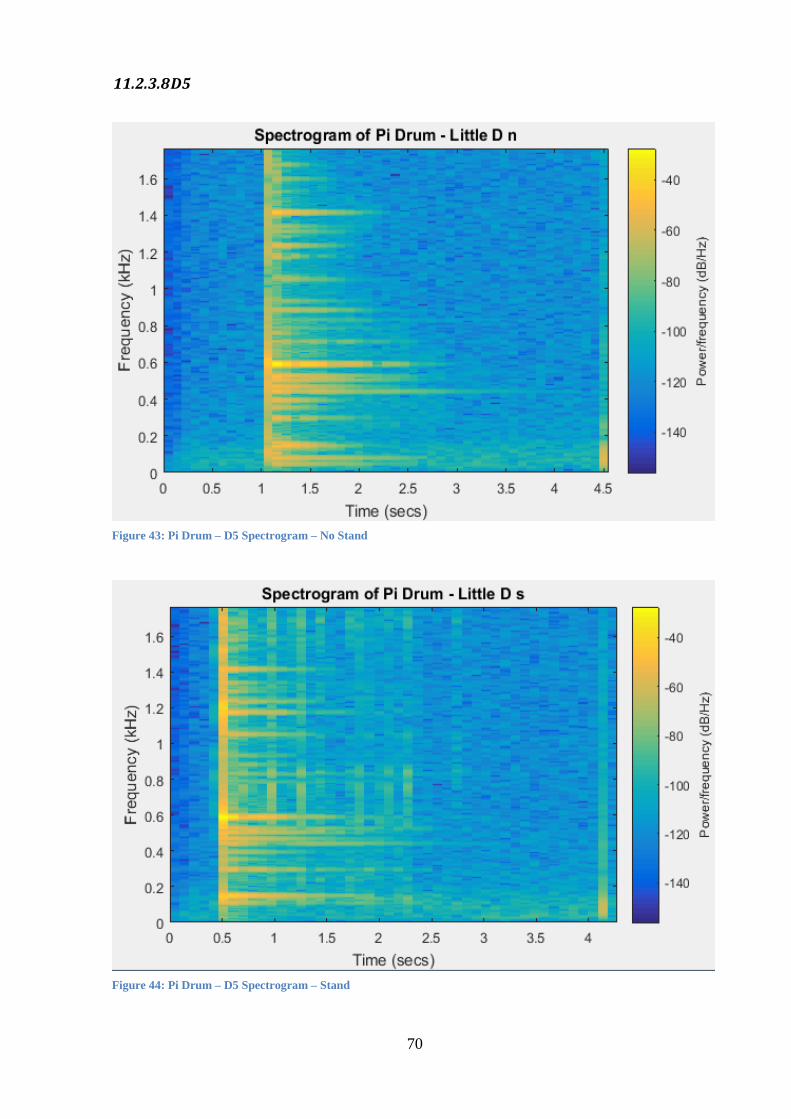
70
11.2.3.8 D5
Figure 43: Pi Drum – D5 Spectrogram – No Stand
Figure 44: Pi Drum – D5 Spectrogram – Stand

71
11.2.4 Meridian Spectrograms
11.2.4.1 G3
Figure 46: Meridian – G3 Spectrogram – No Stand
Figure 45: Meridian – G3 Spectrogram – Stand
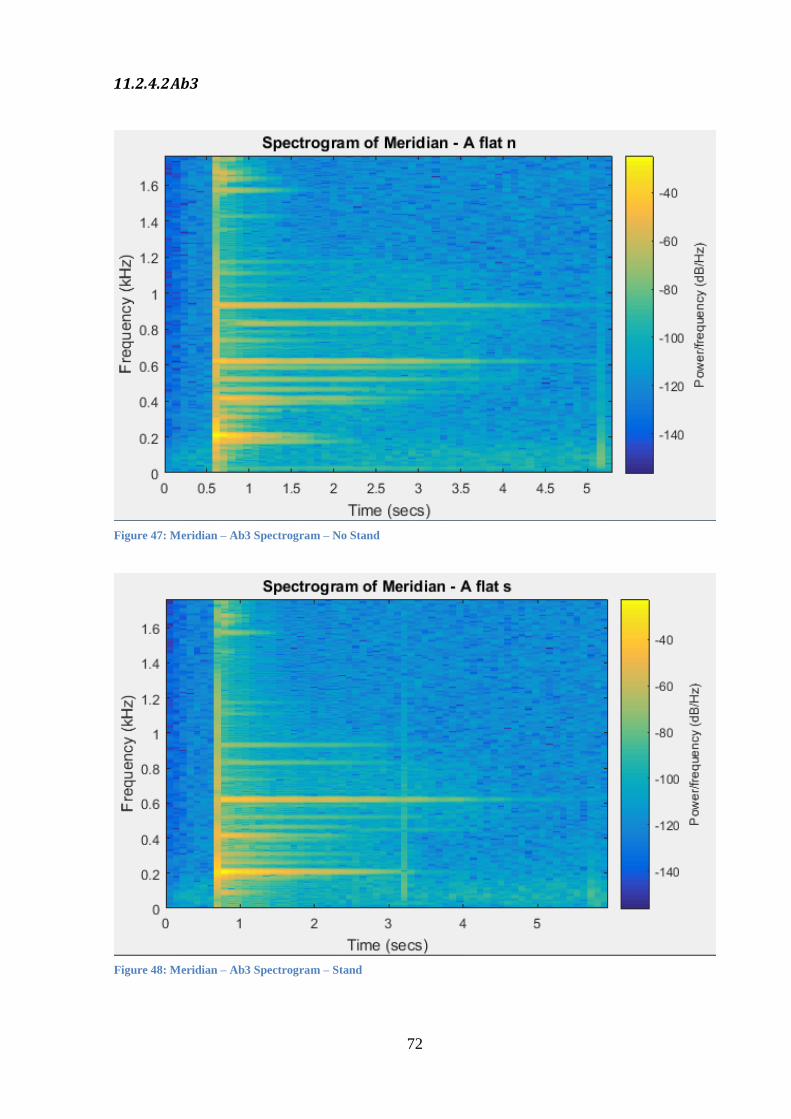
72
11.2.4.2 Ab3
Figure 47: Meridian – Ab3 Spectrogram – No Stand
Figure 48: Meridian – Ab3 Spectrogram – Stand
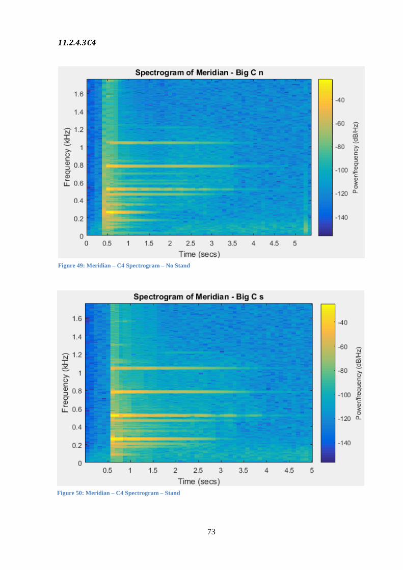
73
11.2.4.3 C4
Figure 49: Meridian – C4 Spectrogram – No Stand
Figure 50: Meridian – C4 Spectrogram – Stand

74
11.2.4.4 Eb4
Figure 51: Meridian – Eb4 Spectrogram – No Stand
Figure 52: Meridian – Eb4 Spectrogram – No Stand
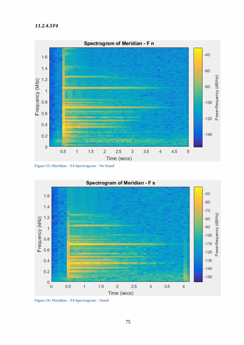
75
11.2.4.5 F4
Figure 53: Meridian – F4 Spectrogram – No Stand
Figure 54: Meridian – F4 Spectrogram – Stand
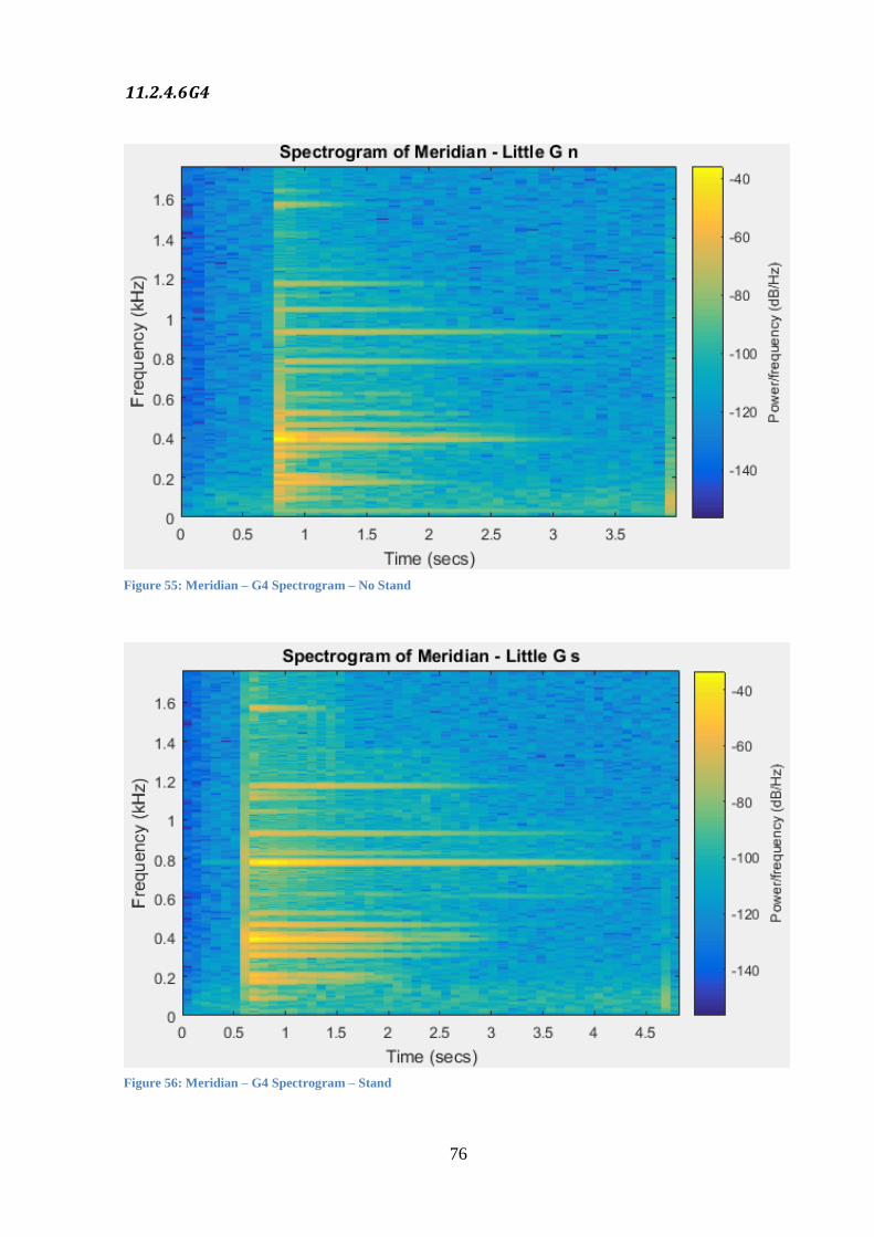
76
11.2.4.6 G4
Figure 55: Meridian – G4 Spectrogram – No Stand
Figure 56: Meridian – G4 Spectrogram – Stand

77
11.2.4.7 Bb4
Figure 57: Meridian – Bb4 Spectrogram – No Stand
Figure 58: Meridian – Bb4 Spectrogram – Stand

78
11.2.4.8 C5
Figure 59: Meridian – C5 Spectrogram – No Stand
Figure 60: Meridian – C5 Spectrogram – Stand

79
11.3 Appendix C
Modelling methods described here were used to create the CAD model of the Pi Drum
instrument used in the report. This method works for instruments that can be divided equally
into parts that contain a single note and has high relevance to all other handpan designs.
1. Divide instrument into equal sections with one note in each section. If equal sections
cannot contain a single note, make the divisions unequal. If equal sized sections can be
used the following describes how to create an easily customised note. This is the same
as Figure 11.
2. Create a sketch of the profile of one half of the instrument if cut through an axis of
symmetry. Do this in two parts; a sketch of the top and bottom shells of the instrument
(Figure 61 and Figure 62).
3. Extrude the sketches in equal amounts from the plane they lie on.
Figure 61: Shell Sketch Bottom

80
4. Create a die/boss in the shape of the note you want (Figure 64).
Figure 62: Shell Sketch Top
Figure 63: Two Way Revolve

81
5. Use the deform feature and the die/boss to push from the inside of the note out to create
the edges and corners of the note (Figure 65).
Figure 64: Die
Figure 65: Die Push

82
6. Use the deform feature to push the remaining curved surface on the note from the
outside in using a created rectangle within the feature (Figure 66).
7. Use the deform feature to create the indent on the note surface. This is done by creating
an ellipsoid and pushing it into the note (Figure 67).
8. Create a set of construction lines that follow the edges on the slice in a plane
perpendicular to the axis is symmetry at the slice tip (Figure 68).
9. Create all notes needed by changing dimensions in steps 4-7.
10. Assemble notes in order. This step can be challenging as solid works does not like
closing a circle. The purpose of the construction lines created on the edge earlier is to
provide a datum for assembly. The author used the axis of symmetry at the tip of the
notes and the construction line to fully constrain the assembly. This only works if the
construction lines are in the same plane, which they will be if the note created is edited
using only steps 4-7.
Figure 66: Flattening Die
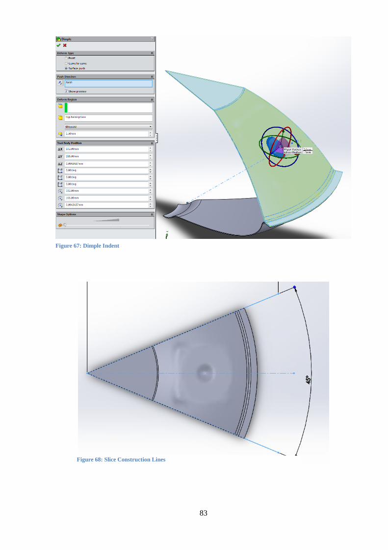
83
Figure 67: Dimple Indent
Figure 68: Slice Construction Lines

84
A brief note. When using the deform feature make sure that faces on both sides of the
material you wish to deform are selected. If they are not, the program will deform only one
face and add or remove material in the space between the other face, which won’t be moved.
ANSYS cannot create a shell element on a geometry with sharp changes from a curve to a
flat surface. This means you must create appropriate transitions in the geometry when
making the sketch of the profile.

85
11.4 Appendix D
11.4.1 Modal Analysis Method
1. Import geometry into ANSYS as a .STEP file and suppress any body that is not part of
the instrument shell.
2. Open Workbench Mechanical and you should have the view shown in Figure 69. Not
all of the items shown will be present as they have to be inserted. The correct contact
region and mesh body sizing and sweep method need to be inserted.
3. The contact region needs to be defined as the contact of the two sections of flat plate on
the edge of the two halves of the shell. Figure 71 shows the set up.
4. The geometry sweep method needs to create solid shell elements and the settings needed
to achieve this are shown in Figure 70.
Figure 69: Modal Project Tree Overview

86
Figure 71: FEA Contact Region Definition
Figure 70: Mesh Sweep Method for Solid Shell Elements

87
5. Refine the mesh on the body with the note as shown in Figure 72
6. Add a fixed support to the surface shown in Figure 73 as well as the edges where the
note would be contacting the rest of the instrument (two of these are also shown).
7. Change Analysis settings to match Figure 74.
Figure 72: Mesh Refinement
Figure 73: Support for FEA
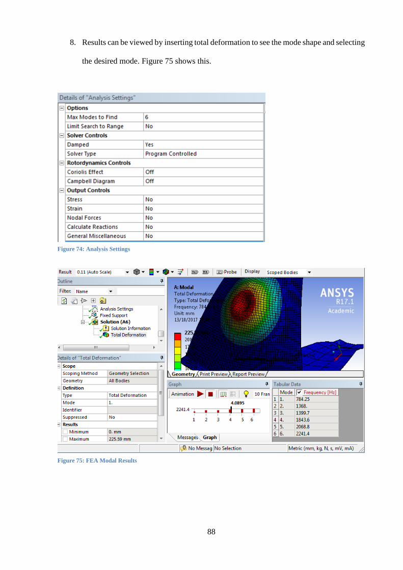
88
8. Results can be viewed by inserting total deformation to see the mode shape and selecting
the desired mode. Figure 75 shows this.
Figure 74: Analysis Settings
Figure 75: FEA Modal Results

89
11.4.2 Transient Analysis Method
Transient Analysis Methodology is as follows:
1. Follow the Modal Analysis method from steps 1-6.
2. Create two named selections as shown in Figure 76. Do this by enabling Node select
and selecting then then inserting the name. The mesh must have been gated to be able
to select a node.
3. Set up the analysis settings as described in 6.3.1 and shown in Figure 78.
4. Apply a nodal force to the point called Load (just above the dimple) with the settings
shown in Figure 77.
5. Solve the model (this often takes multiple hours).
6. Extract the time history for the node named Displacement by inserting a deformation
result in solution. Scope it as a named selection and then select Displacement.
Figure 76: Named Selections

90
Figure 78: Transient Analysis Settings
Figure 77: Nodal Force
Figure 79: Nodal Displacement Time History

91
7. Export the time history displacement data and run it through and FFT to determine
spectral response.
8. Perform steps 1-7 for all notes and desired geometric changes.

92
11.4.3 Transient Analysis FFTs
0
1
2
3
4
5
6
7
8
9
10
200.00 300.00 400.00 500.00 600.00 700.00 800.00 900.00 1000.00
FFT
com
po
nen
t (a
mp
litu
de)
Frequency (Hz)
FFT Transient - D4 Note
Figure 80: FFT of Transient Analysis Time History - D4
0
0.5
1
1.5
2
2.5
3
3.5
4
4.5
5
100.00 150.00 200.00 250.00 300.00 350.00 400.00
FFT
com
po
nen
t (a
mp
litu
de)
Frequency (Hz)
FFT Transient - E4 Note
Figure 81: FFT of Transient Analysis Time History - E4

93
0
1
2
3
4
5
6
7
8
9
10
100.00 200.00 300.00 400.00 500.00 600.00 700.00
FFT
Co
mp
on
ent
(Am
plit
ud
e)
Frequency (Hz)
FFT Transient - F4 Note
Figure 82: FFT of Transient Analysis Time History - F4
0
1
2
3
4
5
6
200.00 300.00 400.00 500.00 600.00 700.00
FFT
Co
mp
on
ent
(am
plit
ud
e)
Frequency (Hz)
FFT Transient - G4 Note
Figure 83: FFT of Transient Analysis Time History - G4
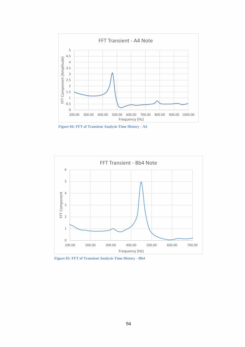
94
0
0.5
1
1.5
2
2.5
3
3.5
4
4.5
5
200.00 300.00 400.00 500.00 600.00 700.00 800.00 900.00 1000.00
FFT
Co
mp
on
ent
(Am
plit
ud
e)
Frequency (Hz)
FFT Transient - A4 Note
Figure 84: FFT of Transient Analysis Time History - A4
0
1
2
3
4
5
6
100.00 200.00 300.00 400.00 500.00 600.00 700.00
FFT
Co
mp
on
ent
Frequency (Hz)
FFT Transient - Bb4 Note
Figure 85: FFT of Transient Analysis Time History - Bb4

95
0
1
2
3
4
5
6
7
8
9
10
200.00 300.00 400.00 500.00 600.00 700.00
FFT
Co
mp
on
ent
(Am
plit
ud
e)
Frequency (Hz)
FFT Transient - C5 Note
Figure 86: FFT of Transient Analysis Time History - C5
0
0.5
1
1.5
2
2.5
3
3.5
4
4.5
5
200.00 300.00 400.00 500.00 600.00 700.00 800.00
FFT
Co
mp
on
ent
(Am
plit
ud
e)
Frequency (Hz)
FFT Transient - D5 Note
Figure 87: FFT of Transient Analysis Time History - D5

96
11.5 Appendix E
0
0.5
1
1.5
2
2.5
3
3.5
4
4.5
5
200.00 300.00 400.00 500.00 600.00 700.00 800.00
FFT
Co
mp
on
ent
(Am
plit
ud
e)
Frequency (Hz)
FFT Transient - D5 Note - No Dimple
Figure 88: FFT - D5 - No Dimple
0
0.5
1
1.5
2
2.5
3
3.5
4
4.5
5
700.00 800.00 900.00 1000.00 1100.00 1200.00
FFT
Co
mp
on
ent
(Am
plit
ud
e)
Frequency (Hz)
FFT Transient - D5 Note - Double Thickness
Figure 89: FFT- D5 - Double Thickness
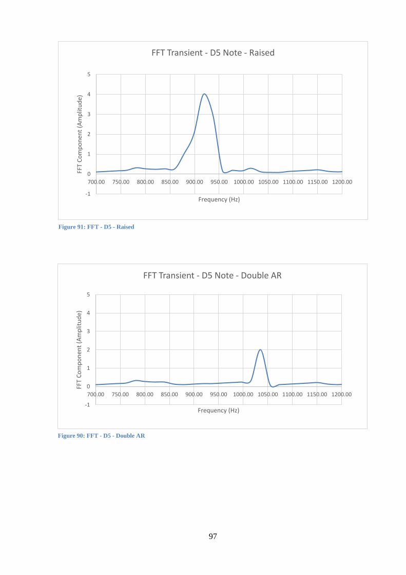
97
-1
0
1
2
3
4
5
700.00 750.00 800.00 850.00 900.00 950.00 1000.00 1050.00 1100.00 1150.00 1200.00
FFT
Co
mp
on
ent
(Am
plit
ud
e)
Frequency (Hz)
FFT Transient - D5 Note - Raised
Figure 91: FFT - D5 - Raised
-1
0
1
2
3
4
5
700.00 750.00 800.00 850.00 900.00 950.00 1000.00 1050.00 1100.00 1150.00 1200.00
FFT
Co
mp
on
ent
(Am
plit
ud
e)
Frequency (Hz)
FFT Transient - D5 Note - Double AR
Figure 90: FFT - D5 - Double AR

98
-1
0
1
2
3
4
5
700.00 750.00 800.00 850.00 900.00 950.00 1000.00 1050.00 1100.00 1150.00 1200.00
FFT
Co
mp
on
ent
(Am
plit
ud
e)
Frequency (Hz)
FFT Transient - D5 Note - Double AR No Dimple
Figure 92: FFT - D5 - Double AR No Dimple
0
0.5
1
1.5
2
2.5
3
3.5
4
4.5
5
700.00 750.00 800.00 850.00 900.00 950.00 1000.00 1050.00 1100.00 1150.00 1200.00
FFT
Co
mp
on
ent
(Am
plit
ud
e)
Frequency (Hz)
FFT Transient - D5 Note - Half AR
Figure 93: FFT - D5 - Half AR

99
0
0.5
1
1.5
2
2.5
3
3.5
4
4.5
5
700.00 750.00 800.00 850.00 900.00 950.00 1000.00 1050.00 1100.00 1150.00 1200.00
FFT
Co
mp
on
ent
(Am
plit
ud
e)
Frequency (Hz)
FFT Transient - D5 Note - Half AR No Dimple
Figure 94: FFT - D5 - Half AR No Dimple