THE UNIVERSITY OF CHICAGO

DEADLINE-BASED GRID RESOURCE SELECTION

FOR URGENT COMPUTING

A THESIS SUBMITTED TO

THE FACULTY OF THE DIVISION OF THE PHYSICAL SCIENCES

IN CANDIDACY FOR THE DEGREE OF

MASTER OF SCIENCE

DEPARTMENT OF COMPUTER SCIENCE

BY

NICK TREBON

CHICAGO, ILLINOIS

JUNE 2008

Abstract

Scientific simulation and modeling often aid in making critical decisions in such di-

verse fields as city planning, severe weather prediction, and influenza modeling. In

some of these situations, the decisions must be made before a strict deadline, after

which the results are of little use. Therefore, it is imperative that these urgent com-

putations begin execution as quickly as possible. The Special PRiority and Urgent

Computing Environment (SPRUCE) aims to provide faster access to computational

Grid resources for urgent computations. Participating Grid resources define local

policies that dictate how urgent computing jobs are handled. For instance, some

resources may kill currently running jobs to allow immediate access, whereas other

resources may only grant next-to-run status. However, the user is still faced with

the challenging problem of resource selection. In particular, the user must select

the configuration (i.e., specification of the computational resource, data repositories,

urgent computing policy and runtime parameters) that will provide the highest prob-

ability of meeting the desired deadline. The purpose of this thesis is to present and

evaluate a set of methodologies and heuristics that generate empirically based, prob-

abilistic upper bounds for the total turnaround time (i.e., file staging, batch queue,

and execution delay) for urgent computations. These upper bounds may then be

used to guide the user in selecting a configuration that offers the greatest probability

of meeting a given deadline. Also provided to guide the user is supplemental data,

such as the current queue state at each resource and the historical reliability of the

computation at a given resource.

ii

Chapter 1

Introduction

Scientific simulation and analysis are often used to guide critical decisions. For ex-

ample, global climate modeling influenced the development of the Kyoto protocol

[1]. Another example is the use of computerized models to aid cities in planning new

freeways or to ease congestion [2]. These examples highlight the importance of sci-

entific simulation and modeling in the decision-making process. However, both these

examples exhibit little urgency in obtaining the results from a computer simulation.

In contrast to these examples is a domain of problems in which there exists only a

brief decision-making window that operates under strict deadlines. Often, in this

domain of urgent computing, late results are useless results. For instance, a tornado

modeling application must provide accurate results with enough warning that the

residents in the target area can seek shelter. Similar situations occur in scenarios

involving wildfires, hurricanes, and tracking of urban airflow contaminants. In order

to meet the deadlines, it is necessary for such urgent computations to access Grid

resources easily and quickly.

The Special PRiority and Urgent Computing Environment (SPRUCE) [3, 4] is a

token-based framework that enables these high-priority urgent computations to effi-

ciently access Grid resources with elevated priorities. Computational resources that

participate are given the flexibility to decide locally how they will respond to urgent

computation requests. However, the problem of resource selection is left to the user.

The user’s primary concern is completing the urgent computation prior to the dead-

line. One method to determine the feasibility of meeting the deadline is to generate a

1

2

probabilistic upper bound on the total turnaround time, which consists of the delay

incurred for any file staging (both input and output), the resource allocation delay

(i.e., batch queue delay), and the execution delay.

This thesis introduces a set of methodologies and heuristics that, taken together,

seek to generate a probabilistic upper bound for a configuration—in other words,

a specification of the data repositories, computational resource, runtime parameters

and policy. These methodologies and heuristics are included as part of the Advisor, a

prototype of a tool that aims to guide an urgent computing user in resource selection.

The Advisor also presents supplementary data, such as the current queue state of

each resource and the historical reliability of the given application on each resource,

that may further aid the user in selecting a resource with greater confidence that the

computation will complete prior to the deadline.

The remainder of this thesis is organized as follows. In Chapter 2, a literature

review of related work is presented. Chapter 3 introduces the SPRUCE framework,

which serves as the context for this work. In Chapter 4, the methodologies and

heuristics that make up the Advisor implementation are introduced. Chapter 5

describes a series of experiments that demonstrate the correctness and utility of the

upper bounds for a case study application. Conclusions are presented in Chapter 6

and future work is detailed in Chapter 7.

Chapter 2

Literature Review

Many current approaches to the Grid resource selection problem seek to reduce the

total turnaround time (or more simply, some aspect of the total turnaround time

such as execution delay or communication cost). However, these approaches are not

suitable for urgent computing. In this domain, there is often little utility in initiat-

ing a computation if a deadline cannot be met. Thus, reducing the total turnaround

time does not directly answer the question of whether the deadline is feasible. Fur-

thermore, the traditional Grid resource selection problem is complicated by the fact

that each resource may have multiple policies in place for handling urgent requests

(e.g., promoting the job to next-to-run status, preemption) that depend on the ur-

gency level of the computation in question. These policies will directly affect how

long an urgent computation waits in a batch queue and, thus, the probability of

meeting a given deadline. In many cases, these policies represent new mechanisms

at a given resource, resulting in a lack of statistical data on which to generate prob-

abilistic bounds. In addition, accurate techniques for bounding the delay for these

policies are necessary despite the fact that actual occurrences of urgent computing

events utilizing these policies may be rare. The remainder of this chapter presents

an overview of a few of the current approaches to the general Grid resource selection

problem and how they can be used to help solve the resource selection problem for

urgent computing.

Schopf [5] presents a brief overview of the tasks a Grid resource scheduler should

perform. The tasks are separated into three classes: resource discovery, system se-

3

4

lection and job execution. Resource discovery includes determining the subset of

machines the given user has authorization for that also meet the minimum neces-

sary job requirements (e.g., OS, RAM, connectivity, disk space). SPRUCE explicitly

handles this step with a warm standby mechanism, which is discussed in Chapter

3.1. System selection tasks consist of gathering dynamic information and selecting a

system based on this information. This is exactly the functionality that the Advisor

provides. Additionally, the Advisor ranks the resources and configurations by the

probability of meeting the deadline. The final stage is execution, which includes

advance reservation, job submission, preparation, monitoring, job completion and

cleanup. Currently, the Advisor is not responsible for scheduling the urgent compu-

tations. Rather, it simply guides the user in resource selection. Schopf raises an issue

about scheduling that SPRUCE should consider: What if the submitted application

is not achieving the predicted performance? One solution is speculative execution

(i.e., submitting the job to multiple resources). Once one copy begins execution, the

remaining jobs can be killed or allowed to complete execution for reliability. While

not explicitly part of the Advisor’s functionality, a poorly performing urgent appli-

cation may result in a reinvocation of the Advisor to select a new resource on which

to run. Thus, the Advisor may be invoked repeatedly.

One approach in Grid resource scheduling is a reputation-based methodology adapted

from the P2P EigenTrust algorithm [6]. Here, entities on the Grid (e.g., users,

resources, or services) have a reputation and trust value associated with them. The

reputation is based on past behavior; the trust value is calculated by examining the

trust of the institution that owns the entity and the trust value of the entity based

on the contexts it supports. The incorporation of reputation and trust serve to

avoid underprovisioned and malicious resources. In the setting of urgent computing,

high levels of trust and reputation are implicit. The set of resources for a given

application is predetermined. In fact, SPRUCE’s warm standby mechanism requires

5

that each potential resource for a given urgent application already have a debugged

and tuned version of that application. Furthermore, the application will have a

validation history of past performance on each resource. Thus, the problem of a

malicious entity is not a concern in the SPRUCE context.

The matchmaking and ClassAds framework employed by Condor [7] attempts to

pair resource requests with matching resources through a classified ads approach [8].

In particular, resources advertise their characteristics, and users advertise their re-

quests. The matchmaker attempts to find matches between these advertisements.

The matchmaker framework attempts to solve some of the problems that occur when

trying to apply traditional resource management techniques to high-throughput en-

vironments (i.e., environments where resources are distributively owned and hetero-

geneous). In SPRUCE, the warm standby resources are the potential matches –

the Advisor needs only to rank them based on both real-time and historical data.

The matchmaker has a ranking feature that evaluates some rank function for each

resource. For the Advisor, this ranking is based on the probabilistic upper bounds

on the total turnaround time for the application on a given resource. The purpose of

this research is to develop the methodology behind generating these bounds.

Liu, et al. [9] extend Condor’s ClassAds language to enable set matching, that is,

to select multiple resources for a single job. Their research deals specifically with

workflows, where multiple interacting components are run on separate computational

resources. Their experiments considered both execution and communication costs.

However, their aim is to select a set of resources that minimizes execution time; their

approach does not provide insight into whether a given deadline will be met. Also,

they do not consider batch queue delay. The research presented here does not include

workflow applications, though this is a domain for future work.

Another approach to Grid resource scheduling is through the use of economic models

6

[10]. In such an approach, a computational economy framework is used for resource

allocation, as well as regulating supply and demand. The computational economy is

derived by charging users the value they get from their results. SPRUCE does employ

a very coarse-grained economic model. SPRUCE users pay a higher price (i.e., a

token) in order to secure higher priority, and they may “shop around” at the resources

to which they have permission to submit urgent jobs in order to find a resource that

offers the best probability of meeting their deadline. The resource providers, in turn,

have a coarse ability to set their price. For instance, a resource owner can charge

a higher price for a preemptive job by granting the priority to a small subset of

urgent computing users. SPRUCE users that do not have permission to submit at

that high urgency level are, effectively, unable to pay that price. Similarly, resource

owners can choose not to offer some priority mechanisms (such as preemption). Also,

resource owners may choose to charge SPRUCE users additional CPU hours for jobs

that receive elevated priority. SPRUCE users will most likely be interested in paying

the minimum possible to meet their deadline; however, a methodology still must be

developed to determine the probability of meeting that deadline.

Nurmi et al. [11] enhance a workflow scheduler to incorporate aspects of batch

queue delay [12] and application performance [13]. Their approach deals specifically

with workflow applications that consist of interacting components that may execute

simultaneously on distinct resources. Similar to the approach outlined in this the-

sis, they make use of a technique that predicts a bound on the amount of delay a

job will experience in a batch queue [12]. Their results show that they are able to

reduce the total turnaround time. In order to estimate the execution time, they

generated a parameterized performance model based on the hardware characteris-

tics of each resource and the application’s behavior (i.e., memory usage and floating

point operations). Communication costs are also included in the model. The pur-

pose of the performance model is not to predict the exact execution time but rather

7

to provide an estimate that can be used by the scheduler to evaluate the effective-

ness of the hardware configuration for the current workflow. While containing many

similarities with the work described in this thesis, there are three primary differ-

ences. First, this thesis proposes an approach that generates a bound on the total

turnaround time in order to determine how likely a given configuration is to meet a

deadline. In contrast, their approach seeks only to minimize the turnaround time,

with no guarantees regarding the deadline. Second, they consider only communi-

cation costs between components and generate predictions using Network Weather

Service probes. TCP-based Network Weather Service probes are inadequate for pre-

dicting large GridFTP file transfers, which is discussed in Chapter 4.1. Finally, their

work is geared to workflow applications consisting of multiple interacting components

whereas our methodology is simplified to a more traditional parallel application that

executes on a single resource.

Chapter 3

Special PRiority and Urgent Computing Environment

(SPRUCE)

The Grid-based SPRUCE architecture is designed to meet the following require-

ments:

• A “session” in which urgent computation jobs may be submitted should be

clearly defined.

• The ability to initiate a session should be easily transferable to avoid a single

point of failure in emergency situations.

• Users associated with a session are able to submit urgent computations to any

permissible resource.

• The framework should support flexible urgent computing policy choices to be

determined and implemented by Grid resource providers.

SPRUCE fulfills these requirements by using a token-based architecture. An urgent

computing session begins with the activation of a token via a web portal or web

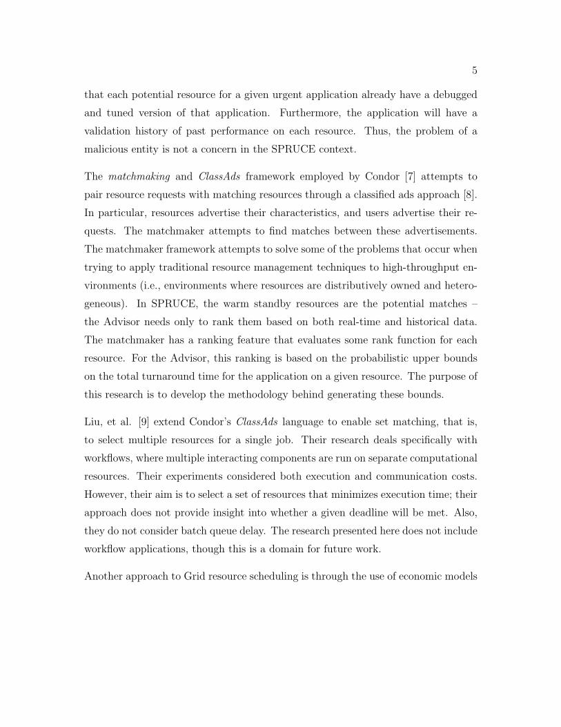
service invocation. Tokens are simply 16-character strings (see Figure 3.1), which

are easily transferable. Furthermore, tokens are created with three static attributes.

First, each SPRUCE token is associated with a set of resources. When activated,

urgent jobs will be granted high-priority access only at these resources. Second, the

token is created with a lifetime, which specifies the duration of the urgent computing

session. Third, each token is created with a maximum urgency level. There are three

8

9

priority levels: red (critical), orange (high), and yellow (medium). Naturally, jobs

with a higher urgency will displace those with a lower urgency when resources are

scarce. Also, multiple levels allow the resource provider to specify multiple responses

based on the urgency of a request. Once a token is created, the token-holder is able

to associate a set of users with the token. Users may be added to or removed from a

valid token at any time. A token is valid once it is created until its session expires.

The associated users have the right to submit elevated priority jobs to any of the

associated resources at the permitted urgency levels.

Figure 3.1: A SPRUCE right-of-way token.

One of the defining design features of SPRUCE is that computational resource poli-

cies are created and implemented by the resource owners. That is, SPRUCE does not

dictate how a resource must respond to an urgent computation request. For instance,

two resources could have the policies depicted in Table 3.1. In this example, Resource

1 has different responses for each urgency level and, as the urgency increases, so does

the response. Resource 2, in comparison, effectively ignores “medium” priority jobs

(i.e., treats them as normal, non-SPRUCE jobs) and handles “high” and “critical”

jobs in a similar fashion. This flexibility allows resource owners to retain ultimate

control over their resources and will lead to an easier adoption of SPRUCE by re-

10

source owners.

Table 3.1: Hypothetical resource policies for urgent computing requests. Policies aredecided locally and not dictated by SPRUCE.

Urgency Resource 1 Resource 2

Medium Elevated queue priority NormalHigh Next-To-Run Next-To-Run

Critical Preemption Next-To-Run

Currently, the scientists must determine the urgency level of their request based

on the perceived importance of their computation. However, it is important that

SPRUCE users adhere to the policies in place at each resource and use good judg-

ment. All urgent computing job submissions are logged, and misuse is handled by

the appropriate system administrators. Such policy issues are outside the scope of

this thesis.

3.1 Warm Standby

In order for emergency applications to be ready for an urgent computation, the

application must be ready for immediate use (i.e., there is no time to test, debug, or

tune the application). Thus, the code must be “frozen” in a ready-to-run state. In

terms of SPRUCE, such an application is said to be in “warm standby.” In a Grid

environment, many potential large-scale computational resources may be available.

Because there is no time to port an application to a new system in an urgent situation,

part of the warm standby process includes selecting a small set of resources that

are well suited for the given application. Furthermore, the warm standby process

includes periodic tests of the application on the selected resources. These tests will

ensure that there have been no underlying changes in the Grid infrastructure (e.g.,

changes to the computational resource environment and GridFTP servers continue

11

to function properly). In addition, periodic testing will also enable performance

monitoring of the application on the various computational resources, which will

be useful for generating bounds on execution delay as well as creating a validation

history.

Chapter 4

Advisor: Deadline-Based Grid Resource Selection

The purpose of this master’s degree research is to develop and evaluate a set of

methodologies and heuristics that can aid a user in resource selection for urgent

computing. This is primarily achieved by generating a probabilistic upper bound on

the total turnaround time for the urgent computation on a particular resource. The

total turnaround time, as depicted in Figure 4.1, consists of the file staging delay

(both input and output), the resource allocation delay (i.e., batch queue delay), and

the execution delay.

Figure 4.1: The four phases of the total turnaround time for an urgent computation.First, any necessary input files are staged to the resource (1). Then, the computationis submitted to the batch scheduler (2). Third, the job executes on the resource (3).Finally, any output file staging is completed (4).

12

13

An urgent computation may have many configurations. A configuration consists of

a single specific instance of an urgent computation. For example, consider an ap-

plication that has three warm standby resources. On each resource it has amassed

performance data for runs on 64 and 128 nodes. The application requires one in-

put file that is available from four different repositories. The application may be

submitted at all SPRUCE urgencies (i.e.,“medium,” “high,” and “critical”) and nor-

mal priority (i.e., no SPRUCE) at each resource where each urgency results in a

distinct policy. Thus, there are 96 different configurations (3 resources * 2 node

specifications * 4 input repositories * 4 policy choices = 96). The user is interested

in knowing which configuration provides the greatest probability of meeting a given

deadline.

For a given configuration, one can predict an upper quantile on the total turnaround

time, which serves as a probabilistic upper bound. For instance, if the 0.95 quantile

for the delay is 100,000 seconds, then there is a 95% chance that the delay will be less

than 100,000 seconds. Each of the individual phases of the total turnaround time

(see Figure 4.1) may be bounded individually: (i) input file staging delay (quantile

IQ corresponds to an upper bound IB ), (ii) resource allocation delay (e.g., queue

delay) (RQ, RB), (iii) execution delay (EQ, EB) and (iv) output file staging delay

(OQ, OB ). In the simple case where each of these phases is independent (i.e., no

overlap), a bound on the total turnaround time can be computed as follows:

An upper IQ x RQ x EQ x OQ quantile corresponding to a bound of

IB + RB + EB + OB .

This composite quantile is conservative in that the composite quantile is at least the

product of the individual quantiles. In reality, this value represents the probability

that all four upper bounds are satisfied individually. For example, if each of the

four individual phases is bounded by an upper 0.95 quantile, then the composite

14

quantile is the upper 0.815 quantile. This corresponds to a probabilistic upper bound

that there is an 81.5% chance all four individual phase upper bounds are satisfied.

Clearly, if each individual bound is exceeded, then the sum of the individual delays

will exceed the composite upper bound. However, this composite quantile does not

include the situations where at least one of the individual bounds is satisfied as well

as the composite bound. This occurs when the overprediction of the satisfied bound

compensates for the underprediction of the individual bound or bounds that are

exceeded. In the context of urgent computing, this conservativeness is acceptable,

as it is better to err on the conservative side in order to reduce the chances that the

results are produced after the deadline.

In the following three subsections, the methodology for predicting the individual

phase quantiles is presented. For the most part, these calculations use pre-existing

technologies. The novel contributions and uses of this research will be highlighted.

4.1 Input and Output File Staging Bounds Prediction (IQ,

IB and OQ, OB)

The underlying methodology for bounding the input and output file staging delays

(phases 1 and 4 in Figure 4.1) is the same. In the case of multiple input or output

files that originate from a single source or are transferred to a single destination, it

is preferred to transfer the input or output data as a single bundled transfer. This

procedure will avoid lowering the overall quantile that occurs when the quantiles are

combined to generate a composite upper bound.

The predicted upper bound for the output file staging delay suffers from an inherent

obstacle, namely, that the predictions are based off the current network bandwidth

but the actual file transfers will not occur until some later point in time (i.e., after

15

the conclusion of the input file staging, resource allocation and execution phases).

The greater the span of time between the prediction and actual transfer, the greater

the probability that the bandwidth behavior may have changed. Part of this research

examines how the performance of these predictions fare in a case study application

(see Chapter 5) where the output file staging occurs 2–15 hours after the predictions

are made.

The Network Weather Service (NWS) provides the necessary functionality to peri-

odically measure the bandwidth between a source and destination and make pre-

dictions on expected bandwidth [14]. Furthermore, a probabilistic upper bound can

be created for some measurement streams by using the mean square error (MSE)

as a sample variance of a normal distribution and then calculating the upper con-

fidence interval. For example, one can calculate the upper 95% confidence interval

as forecast + 1.64 ∗√

MSE. However, complications arose while trying to predict

the bandwidth achieved for GridFTP transfers using the TCP-based NWS probes.

In many cases, particularly involving sources and destinations that were part of the

TeraGrid [15] that exhibited high bandwidth rates, the probes were unable to match

the bandwidth behavior achieved by the GridFTP transfers. For an example of this

problem, see Figure 4.2. Here, the transfers exhibit much more variability and a

higher peak bandwidth. The transfers also exhibit more of a bimodal appearance.

Moreover, the probes and transfers both appeared to be traveling the same path

from source to destination and modest attempts at scaling up the probe size were

not helpful. In another experiment, the size of the file used in the GridFTP transfers

was modified to match the size of the probes. In Figure 4.3, the results of one such

experiment are shown. As before, the transfers exhibit a bimodal behavior and a

higher peak bandwidth. One tool that was useful in comparing the bandwidth series

was ts comp [16]. This tool uses techniques that remove differences in shift and scale

while comparing one time series with another. In many cases, however, the tool was

16

unable to report a similarity matching between a probe series and the corresponding

GridFTP transfer series.

Figure 4.2: On the left is a plot of the bandwidth achieved by 1,049 2 MB TCP-basedprobes that are sent every 15 minutes between the Indiana input source and Mercury.On the right are the corresponding transfers of a 171 MB file that is transferred viaGridFTP every 15 minutes.

The above data clearly indicates that the small TCP-based probes used by NWS

are unable to match the behavior of GridFTP transfers. As a result, a GridFTP

probe framework was implemented that periodically measures the bandwidth be-

tween the source and destinations by transferring probes via GridFTP. These probes

were individually tuned for each source-destination pair until the probe bandwidth

and transfer bandwidth were similar. The GridFTP framework produced results that

more closely matched the behavior of the actual GridFTP transfers. An actual NWS

17

Figure 4.3: On the left is a plot of the bandwidth achieved by 154 2 MB TCP-basedprobes that are sent every 15 minutes between the Indiana input source and Tung-sten. On the right are the corresponding transfers of a 2 MB file that is transferredvia GridFTP every 15 minutes between the source and destination.

18

installation is still used to track each series and generate the necessary probabilistic

bounds based on those probes.

4.2 Resource Allocation Bounds Prediction (RQ, RB)

The resource allocation delay (phase 2 of Figure 4.1) represents the amount of delay

from when a job is submitted to a resource until it begins execution. One of the pri-

mary methods that SPRUCE uses for urgent computing is reducing the batch queue

delay through elevating the priority of urgent computations. However, the amount

of queue delay an urgent computation will experience depends not only upon the re-

source load, but the local policy that each resource implements for the given urgency

level. This policy details how urgent requests are handled. Currently, two policies

have been implemented, other than the normal (i.e., no SPRUCE) priority:

1. Next-to-run – The job is designated as the next job to run.

2. Preemption – If necessary, jobs that are currently executing are killed to free

up the necessary resources for the preemptive job.

In order to generate the probabilistic bounds for the normal priority resource al-

location delay, the existing Queue Bounds Estimation from Time Series (QBETS)

[17] technology is used. This service is already included in the TeraGrid portal. At

the heart of the QBETS methodology is a technique the authors call the Binomial

Method Batch Predictor (BMBP) [12]. For computations that are submitted at a

normal priority, QBETS can be queried for a desired upper quantile. Currently,

the tool supports the upper 0.95, 0.75, and 0.50 quantiles for a given resource and

queue.

19

For the next-to-run priority, the authors of QBETS have modified their tool in order

to generate bounds for next-to-run jobs. In the modified tool, a Monte Carlo simula-

tion of next-to-run batch queue delays is conducted based on previously observed job

history. This simulation produces a distribution of next-to-run delays for a number

of different job sizes. From these distributions, the tool predicts bounds on the next-

to-run delay for a job using the same internal software infrastructure as the original

QBETS. Part of the purpose of this research is to validate this methodology for the

next-to-run priority. Also, it is the first example of using this bounds generator in

the context of resource selection.

For the preemption policy choice, the authors of QBETS have extracted the BMBP

methodology that is at the heart of QBETS to create a tool that can be applied to

an unknown distribution rather than a time series. This tool is then used to predict

bounds on the preemption delay based on previously observed preemption delays for

similarly sized jobs. This research is the first to attempt to use this methodology in

such a manner. The methodology appears to be a good fit because it is nonparametric

and general.

The probabilistic bounds generated for the preemption policy involve a number of

assumptions. For example, it is assumed that there are enough nodes available to

preempt. In two cases, this assumption may not hold. First, there may not be enough

responsive nodes available to preempt; for example, if a resource has 64 nodes but

10 nodes are down, it will not be able to allocate a preemptive job requesting more

than 54 nodes. Second, depending on the policy, preemptive jobs may not be able

to preempt other preemptive jobs (such is the case at the UC/ANL IA-64 TeraGrid

resource). In this case, a preemptive job will wait in the queue until there are enough

nodes freed up by the completion of earlier preemptive jobs. In such a scenario

it is assumed that the bounds predicted will be incorrect. Also, the preemptive

bounds generated by this method assume that a resource is completely used. In

20

other words, the history used by the methodology only includes samples of when all

the requested nodes had to be preempted. In practice, some of the requested nodes

may already be free, resulting in a shorter preemption delay because fewer nodes are

being preempted.

Several situations may arise in which the above methodologies will perform poorly.

For example, consider the case where a resource is idle and the requested nodes are

immediately available. In this situation, a job could be submitted with no SPRUCE

urgency and begin executing almost immediately. However, the bounds generated for

the various policies would most likely be excruciatingly conservative despite the fact

that this scenario is clear from the current state of the resource. This situation occurs

because the above methodologies generate resource allocation bounds based on past

job history and not on the current queue state. As another example, consider the

situation where it is clear from the queue state that there may be a queue delay that

exceeds the predicted upper bound. Such an instance may occur for a normal priority

job when a massive job is submitted that requests most of the nodes begins executing

before the urgent computation. For a SPRUCE job, a similar situation arises when

other SPRUCE jobs of the same or higher priority are submitted prior to the job in

question. These situations are a direct result of predictions that are based entirely off

of historical data. While the historical data may provide correct predictions from a

mathematical standpoint, there may be cases where simple inspection of the current

state may provide additional insight. For resources using the Globus toolkit, the

current state of the resource may be available via the Monitoring and Discovery

Services framework (MDS) [18]. This framework allows for the current state of

participating resources to be discovered via a web service call. Thus, by reporting

back both the probabilistic bound and the current state of the resource, a user can

ascertain whether such situations exist.

21

4.3 Execution Bounds Prediction

Similar to preemption batch queue bound predictions, the modified BMBP tool is

again used to generate probabilistic upper bounds on the execution delay (phase 3

in Figure 4.1). Again, the present research is the first to use this methodology to

predict an upper bound on execution delay. This approach exploits the fact that

the warm standby mechanism will be creating a log of periodic executions of the

application on typical input sizes in order to validate that the application is ready

for urgent use.

4.4 Improving the Composite Quantile and Bound

As mentioned, the composite quantile is conservative in that it represents the prob-

ability that the delay for each of the individual phases (i.e., file staging, resource

allocation, and execution) is satisfied. Even when targeting high quantiles for the

individual phases, the composite quantile quickly decreases (e.g., targeting the 0.95

quantiles for input file staging, resource allocation, execution and output file staging

results in the composite 0.815 quantile). However, the composite quantile can be

increased, either through overlapping phases of the urgent computation or through

speculative execution. Each of these approaches is briefly discussed below.

4.4.1 Overlapping Phases of the Urgent Computation

In the above formulation of the composite upper bound, the clause of independence

requires that the four phases occur one at a time (e.g., no overlap). By requiring

phase independence, however, one ignores a relatively straightforward opportunity to

both reduce the composite bound and increase the corresponding quantile. The most

22

obvious opportunity for overlap is by staging the input files while the job is waiting

in the batch queue (see Figure 4.4). Clearly, the application must be able to handle

the situation in which it begins execution before the input data arrives. A simple

solution (though potentially wasteful in terms of unnecessary cycles) is to have the

application “spin” until the input is available. In this situation, any time that the

application spends in the queue while data is being transferred is an actual decrease

in the overall delay of the total turnaround time. However, the primary benefit

is in the calculation of the bound. Consider the following example. For a given

urgent application, the input files have a probability of 0.90 of being transferred in

10 minutes, a probability of 0.95 of being transferred in 20 minutes, and a probability

of 0.99 of being transferred in 30 minutes. Similarly, the job has a probability of 0.75

of beginning execution in 10 minutes, a probability of 0.85 of starting execution

in 20 minutes, and a probability of 0.95 of starting execution in 30 minutes. In the

serial case, one could generate a composite 0.90 quantile by combining the individual

0.95 quantiles; in this case, that is an upper 0.90 quantile of 50 minutes. But, in

the overlapping case, if the target job start time is the 0.95 quantile of 30 minutes,

there clearly is a probability of 99% that the files will be done transferring in 30

minutes. Thus, the composite upper bound in this case is actually the 0.94 quantile

of 30 minutes. In comparison to the serial case, we decreased the bound (30 minutes

rather than 50 minutes) while increasing the quantile (0.94 versus 0.90). In general,

for two phases that overlap completely (i.e., start at the same time), the composite

upper quantile is the product of the two individual quantiles. and the corresponding

bound is the maximum of the two individual bounds.

23

Figure 4.4: Timeline for the serial and overlapping phases of an urgent computation.In I, the phases are serial. In II and III, the input and resource allocation phasesare overlapped. In II, the input phase completes prior to completion of the resourceallocation phase. In III, the resource allocation phase completes prior to the end ofthe input file staging phase. In this case, the portion of time from when the resourceallocation phase ends until the input file staging phase ends represents wasted cycles,where the computation “spins” until the input is ready.

24

4.4.2 Speculative Execution of Independent Configurations

In Chapter 2, Schopf suggests speculative execution as a means to increase reliabil-

ity. In terms of urgent computing, submitting multiple, independent configurations

simultaneously can improve the probability of meeting the deadline for at least one

of the configurations. Consider the case where a user simultaneously initiates two

independent configurations of an urgent computation. If the first configuration has

a probability of Pr(config1) of meeting the deadline and the second configuration

has a probability of Pr(config2) of meeting the deadline, the probability that at

least one of the configurations meets the deadline is Pr(config1) + Pr(config2) −Pr(config1)Pr(config2). This formulation requires that config1 and config2 be

independent events. Specifically, it requires that neither configuration utilizes the

same input repository, computational resource, or output repository.

4.5 Optimizing the Probabilistic Bound for a Configuration

The above methodology describes how to generate a conservative composite upper

bound on the total turnaround time for an urgent computation configuration. The

composite quantile consists of the product of the individual phase quantiles. Clearly,

by computing a different quantile for an individual phase, the composite quantile

and bound will change as well. Thus, to determine the “optimal” probabilistic up-

per bound, the Advisor needs to find the combination of individual quantiles that

generates the highest quantile that corresponds to a bound less than the deadline. It

is more advantageous to maximize the probability rather than minimize the bound

because the urgent-computing user is most interested in the probability of meeting

the deadline. For example, if the deadline is in six hours, it is more useful to know

that there is a 75% chance of the urgent computation completing in five and a half

25

hours rather than a 20% chance of finishing in less than two hours. The current

methodology implemented by the Advisor is to query a small set of points for each

phase and then consider all possible combinations. The highest composite quantile

with a bound less than the deadline is then associated with the given configuration.

If no such quantile exists, then that configuration may be ignored as the calculated

probability of meeting the deadline is small. Then, the remaining configurations are

presented to the user with their associated probabilities.

4.6 Limitations of the Composite Bounds

The composite upper bounds generated for this research have a number of limita-

tions. First, an urgent computation is assumed to consist of a traditional parallel

code rather than a workflow comprising of multiple interacting components that exe-

cute simultaneously on distinct resources. Second, the probabilistic bounds that are

generated correspond to the probability of a single instance of the urgent compu-

tation. These bounds are not valid for multiple instances of the configuration. For

example, if a user simultaneously submits 100 instances of a single urgent computa-

tion configuration, the bound is not valid for all of the instances. In such a scenario,

the inherent correlation is not addressed by the predicted bounds. This situation is

different from the speculative execution scenario in which independent configurations

are submitted simultaneously; in the latter case, there is little correlation.

Chapter 5

Case Study

In order to evaluate the methodologies just described for generating composite upper

bounds on the total turnaround time, experiments were conducted using FLASH [19]

as a sample scientific simulation. FLASH is a modular, multiphysics, adaptive-mesh

astrophysics code developed at the University of Chicago Astrophysics Department.

It is used to study a variety of astrophysical phenomena and has scaled on some of the

largest high-performance computing systems in the world. The “cellular” problem

used for this research involves the material flows during nuclear burning. The case

study application executes 1,000 time steps using eight levels of mesh refinement.

While FLASH may not be an ideal urgent computing application, it was selected

because it is an example of a well-known scientific computing code with a high level

of local expertise (i.e., University of Chicago).

The FLASH code was ported to the three TeraGrid resources listed in Table 5.1,

which served as the set of warm-standby resources. In order to seed the execution

bounds predictor for each resource, 100 trials of the application were completed on

each resource, and their execution delays (as reported by the various batch queue

logs) were recorded.

Table 5.1: The three warm standby resources for the case study application.Name CPU Nodes CPUs

UC/ANL IA-64 Itanium 2 Madison (1.3/1.5 GHz) 62 124Mercury (fastcpu) Itanium 2 (1.5 GHz) 631 1262

Tungsten Intel Xeon (3.5 GHz) 1280 2560

26

27

While the FLASH simulation does not require any file staging, this requirement was

artificially added into the case study in order to create a full urgent computation that

consists of all four phases of delay (i.e., input file staging, batch queue, execution and

output file staging). The data movement requirements were loosely modeled after

the requirements of a Linked Environments for Atmospheric Discovery (LEAD) [20]

workflow. LEAD is one of the first users of the SPRUCE framework, and in 2007 the

team worked with SPRUCE to perform real-time, on-demand, dynamically adaptive

forecasts [21]. For the case study, a 3.9 GB input file is required prior to execution.

The input data is available via GridFTP from two locations, the University of Indiana

and the University Corporation for Atmospheric Research (UCAR). The (artificial)

output data is similarly sized and must be transferred to a server at the University

of Indiana.

The case study consists of the six experiments outlined in Table 5.2. The remainder

of this chapter discusses each experiment and its results.

5.1 Experiment 1: GridFTP

The purpose of the first experiment was to validate the upper bounds for the input

file staging phase for the UCAR input repository. The configurations that consisted

of the UCAR input repository were omitted from later experiments in order to reduce

the overall number of complete trials of the case study that were completed. If the

bounds for the input file staging phase are correct, as well as the bounds for the

resource allocation, execution, and output file staging phases of later experiments,

one can infer that the total turnaround time bounds most likely would have been

correct as well. The UCAR host resides outside the TeraGrid network, and the

transfers were significantly slower than those originating from the alternative input

repository at Indiana. In this experiment, the upper 0.95 quantile was predicted for

28

Table 5.2: Brief description and purpose of each of the experiments in the case study.

# Name Description Purpose

1 GridFTP Test predicted bounds Validate the methodology forfor GridFTP transfers. bounding GridFTP transfers

from UCAR input source.2 Normal Test configurations Evaluate composite methodology

utilizing normal performance on normal priority.(i.e., no SPRUCE)priority.

3 Next-to-run Test configurations Evaluate composite methodologyutilizing next-to-run performance on next-to-runpriority. priority. Further validate

next-to-run bounds predictor.4 Preemption Test configurations Evaluate composite methodology

utilizing preemption performance on preemptionpriority. priority. Validate preemption

bounds predictor.5 Overlap Test configuration Evaluate gains from

with overlapping overlapping input and queuephases. phases.

6 Advisor Test approximate Demonstrate algorithm tooptimization of optimize composite quantilequantile methodology. and discuss results.

29

the transfer of a GridFTP file from the UCAR host to each of the three case study

resources (see Table 5.1). This procedure was repeated at least 100 times in order to

track the success rate. The results of these experiments, summarized in Table 5.3,

indicate that the methodology is doing a reasonable job in generating an accurate

and relatively tight upper bound.

Table 5.3: Results from experiments generating an upper 0.95 quantile bound on thedelay achieved in a large GridFTP transfer from the UCAR input source to one ofthe case study resources. The transferred file was 3.9 GB.

Destination # of Trials Percent < Bound Percent Overprediction

UC/ANL IA-64 112 100 8.5Mercury 113 91.2 4.90Tungsten 364 95.9 25.89

5.2 Experiment 2: Normal Priority

The purpose of the second experiment was to validate the correctness of the bound

methodology for the total turnaround time for configurations using normal prior-

ity. For this experiment, both the individual and composite bounds for the normal

priority (i.e., no SPRUCE) configurations on all three resources were studied. Be-

cause the UC/ANL resource is much smaller, the application runs on 16 nodes with

2 processors per node, whereas 32 nodes with 2 processors per node are requested

for Tungsten and Mercury. In these configurations, the Indiana source was used for

input file staging. For each of the individual phase bounds, the upper 0.95 quan-

tile was predicted. Thus, the resulting composite bound represents the upper 0.815

quantile (i.e., 0.954 = 0.815).

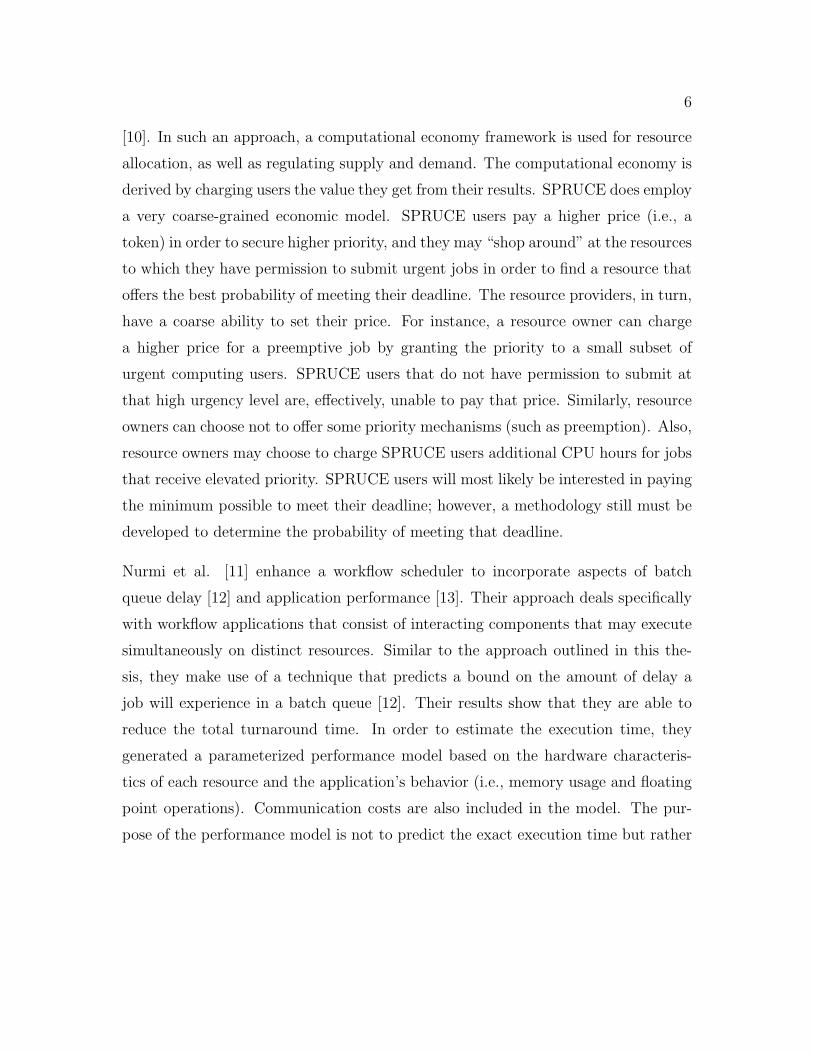
The composite upper bounds and actual delays from the three configurations are

depicted in Figure 5.1. For the UC/ANL IA-64 resource, the predicted bounds

30

Figure 5.1: Predicted upper 0.815 quantile versus the actual the delay achievedby the configurations using the Indiana input source and normal priority for theUC/ANL IA-64, Mercury and Tungsten resources. Note the different scales betweenthe UC/ANL resource and Mercury/Tungsten.

experience a significant drop midway through the experiment and closely follow the

actual delays (see Figure 5.1). This is caused by the underutilization of the resource.

In this experiment, 72 of the 99 completed runs experience a queue delay of one

second or less. In addition, much of the time the only job queued on the resource

was the case study job. These factors combined to create a bias in the predicted

bounds because the stream of case study jobs was submitted during a period of

low activity on the resource. Hence, a change point in the batch queue delay time

series was detected by QBETS, and the predicted delays were drastically reduced.

However, the data still shows that the predicted upper bound is serving its purpose

in that the target probability of overall success is being met.

The results of the individual phase upper bounds as well as the overall bounds are

summarized in Table 5.4, and the overprediction percentage for each phase is listed

in Table 5.5. The success rate of the input file staging bounds for Tungsten is only

31

88%. However, several factors contributed to the low success rate. First, during the

experiments, the dedicated Tungsten GridFTP server was experiencing problems that

would not allow incoming connections. Hence, few probes were completed, thereby

hindering the bounds predictions. After 15 runs, the experiments were shifted to use

the login nodes as the GridFTP server. While this strategy eliminated the connection

problem, it introduced another: the performance was a lot more variable as the

server was no longer dedicated solely to handling GridFTP traffic. This variability

was evident in the both the probes and actual transfers.

Table 5.4: Percentage of measurements that were less than the predicted upperbound for the configurations using the Indiana input source and normal priority. Forthe individual phases (i.e., input, queue, execution, and output), the target quantilewas 0.95; for the overall bound, the quantile was 0.815.

Resource # of Trials Input Queue Execution Output Overall

UC/ANL IA-64 99 100% 97% 100% 83% 97%Mercury 100 99% 99% 93% 86% 100%Tungsten 100 88% 99% 96% 77% 99%

Table 5.5: Percent overprediction for each phase of the configurations using theIndiana input source and normal priority.

Resource Input Queue Execution Output Overall

UC/ANL IA-64 7.98% 2,379.09% 7.01% 21.89% 64.95%Mercury 10.19% 4,468.23% 3.78% 5.29% 1,417.26%Tungsten 10.57% 4,811.20% 13.03% -4.63% 1,842.43%

The upper bounds for the queue phase all exceed their target 95% hit rate. However,

the overprediction percentage clearly shows that the bounds are not very accurate.

This problem arises from the variability in batch queue delays. For example, as

mentioned above, most of the time (72 out of 99 trials) the batch queue delay in the

UC/ANL IA-64 configuration was one second or less. However, three queue delays

were more than 6,900 seconds, including one that lasted over 10,800 seconds. In the

32

case of Mercury and Tungsten, the overprediction rate is even worse, as they both

exceed 4,000%.

The execution bounds for all three phases do particularly well in terms of correctness

and tightness. Both the UC/ANL and Tungsten resources exceed the target 95%

success probability, with Mercury performing just below at 93%. The overprediction

rates are also reasonable, at less than 14%. These results indicate that the BMBP tool

is performing well, thus supporting its use as the execution delay bounds predictor.

Again, one of the reasons it was selected was its general nature. This is highlighted

by the UC/ANL resource, which consists of processors of two different clock speeds

(1.5 and 1.7 GHz). As a result, the execution delay is bimodal, yet these results

show not only a 100% success rate but also a very tight bound.

The results for the output phase are also promising. First, this phase possesses the

inherent challenge that the bounds predictions are made for the bandwidth at a given

point in time, but the transfer is not initiated until some later point. Even if there is

no significant queue delay, the predictions are still for some point two to three hours

in the future for this experiment. And, in the worse case, the output phase did not

begin until more than 12 hours after the predictions were made. For the UC/ANL

IA-64 resource, all 17 misses (as seen in Table 5.4) occurred in a span of 18 trials.

During this time, there was a problem with the probe framework and practically no

probes were getting through. The result was that the bounds predictions were not

adjusting to the current bandwidth. Once the probes began getting through, the

predicted bounds were not exceeded in any of the remaining 70 trials. For Mercury,

two of the output transfers actually failed because one of the GridFTP servers did

not allow a connection. The remaining 12 misses were often the result of making

predictions for transfers occurring in the future. This was evident in the data, where

often after one of the misses, the prediction for the output bound of the subsequent

trial would see a large increase. This corresponds to the probes detecting a change in

33

the network bandwidth and adjusting the bounds—an adjustment that would occur

during the trial in question but not be reflected in the predicted upper bound. In the

case of Tungsten, the problems with the GridFTP servers were previously discussed.

Nine of the misses occurred while using the misbehaving dedicated server, which

experienced very few probes getting through. The remainder of the misses occurred

while using the more variable login node as the GridFTP server.

The overall bounds perform well, in terms of correctness. Each of the resources ex-

perience a success rate greater than 96% while the conservative target rate is only

81.5%. The reason for the success was due primarily to the conservative nature of

the batch queue bounds. Often, the predicted batch queue bound was nearly as

large as the actual delay of the total turnaround time. For these experiments, the

overprediction of the batch queue phase always accounted for the misses in other

phases. The average delay for each configuration along with the average predicted

bounds are presented in Table 5.6. The conservative nature of the bounds is partic-

ularly evident for Mercury and Tungsten, where the bounds are more than an order

of magnitude larger than the actual delay.

Table 5.6: Average delay and bound (in seconds) for the total turnaround time ofthe configurations using the Indiana input source and a normal priority.

Resource Average Delay Average Bound

UC/ANL IA-64 10,833 17,869Mercury 8,696 131,951Tungsten 7,631 148, 233

The results of this experiment indicate that the composite bounds are correct but

not very accurate. The primary reason for the inaccuracy is the overprediction of the

batch queue delay bounds. This is a result of the inherent variability in batch queue

delay for highly used computational resources. However, this inaccuracy was also

evident in the relatively underused UC/ANL resource. This overprediction is also

34

an implicit argument for SPRUCE, which aims to reduce batch queue delay through

elevated priority. As a result, the bounds for SPRUCE jobs should be lower and

tighter than the bounds generated for normal jobs.

5.3 Experiment 3: Next-To-Run Priority

The purpose of the third experiment was to further validate the next-to-run bounds

predictor and demonstrate the utility of the composite bounds for a SPRUCE ur-

gent computation. The next-to-run experiment consisted of using the Indiana input

source, UC/ANL IA-64 resource (16 nodes with 2 processors per node), and an ur-

gency level of “high.” At this point, there was an execution history of roughly 200

trials, 100 to seed the bounds predictor and 100 trials from the normal configuration

experiment. Because the execution bounds in the previous experiment performed

well, the execution delay for this experiment was emulated by randomly sampling

the execution history. The aim was to avoid the needless wasting of CPU cycles by

continually running the case study application. In order to generate valid queue de-

lays, however, a dummy job (e.g., hello world) was submitted to the batch scheduler

requesting the same number of nodes and wall clock time as before. Once the dummy

job finished execution, the execution delay was sampled and the case study urgent

computation slept for the appropriate time. As was the case in the normal config-

uration experiments, the 0.95 quantile was predicted for the four individual phases,

with the resulting composite 0.815 quantile for the total turnaround time.

The predicted bounds plotted against the actual delay are shown in Figure 5.2.

Here, the projected bounds are much tighter than in the previous experiments using

normal priority. In all, 98 trials of this configuration were completed. The results of

the predicted bounds are summarized in Table 5.7, and the overprediction percentage

for each phase is listed in Table 5.8.

35

Figure 5.2: Predicted upper 0.815 quantile versus the actual delay achieved bythe configuration using the Indiana input source and next-to-run priority for theUC/ANL IA-64 resource.

Table 5.7: Percentage of measurements less than the predicted upper bound forthe configuration using the Indiana input source, next-to-run priority, and UC/ANLresource. For the individual phases (i.e., input, queue, execution, and output), thetarget quantile was 0.95; for the overall bound, the quantile was 0.815.

Resource # of Trials Input Queue Execution Output Overall

UC/ANL IA-64 98 100% 92% 91% 92% 94%

Table 5.8: Percent overprediction for each phase of the configuration using the Indi-ana input source, next-to-run priority, and UC/ANL resource.

Resource Input Queue Execution Output Overall

UC/ANL IA-64 8.04% 46.37% 4.54% 41.47% 11.27%

36

With the next-to-run priority, the success rate of the upper bound for the queue

phase is just under 92%. However, all of the misses occurred at the beginning of the

experiment (in the first 20 trials). During this time, there was a burst of activity

on the resource, including the submission of 25 8-hour, 8-node jobs. The result

was that the next-to-run jobs would actually have a nontrivial batch queue delay.

However, this delay was smaller than if the case study job had been submitted as

a normal job. In that case, that job would have most likely waited until nearly all

of the 8-node jobs had finished. There was also a single 24-hour job submitted that

requested enough nodes such that the next-to-run job could not begin. In the plot,

this corresponds to the single large spike of the actual delay which occurred when the

job waited in the queue for over 13 hours. Noteworthy, however, is the fact that the

overprediction percentage has dropped to roughly 46%, a substantial improvement

on the overprediction rate that occurred for the normal configuration on the same

resource.

For the total turnaround time bounds, a success rate of nearly 94% was achieved

with a significantly smaller overprediction rate than achieved in the normal prior-

ity experiments. These results clearly indicate that the composite bounds are not

only correct but also more accurate. Moreover, the results offer further validation of

the next-to-run bounds predictor, which is producing correct bounds that are signifi-

cantly tighter than the normal priority bounds. Consequently, the composite bounds

are also much tighter, which is evidenced by the fact that the average trial had a

delay of 11,562 seconds and the average composite bound was 12,966 seconds.

5.4 Experiment 4: Preemption Priority

The purpose of the preemption experiment was to validate the bounds prediction

methodology for the preemption policy. This experiment consisted of the configu-

37

ration using the Indiana input source, UC/ANL IA-64 resource (16 nodes, with 2

processors per node) and urgency level of “critical.” As was the case in the normal

configuration experiments, the 0.95 quantile was predicted for the four individual

phases, with the resulting composite 0.815 quantile for the total turnaround time.

The preemption bounds were generated from a history of 100 preemption trials that

were used to seed the bounds generator. In order to avoid the clear impact on jobs

outside of the case study, both the 100 preemption seed trials and the trials for this

experiment were conducted as follows. First, a job was submitted that requested

the necessary number of nodes (i.e., 16). Then, a preemptive job was submitted to

the same set of nodes. This avoided the unnecessary killing of outside jobs. For this

experiment, the dummy job was submitted and allowed to begin execution prior to

the bounds predictions and initiation of the trial. As in the next-to-run case, the ex-

ecution delay for the preemptive job was emulated from the execution history.

The plot of the actual delay versus the predicted bounds is depicted in Figure 5.3.

In all, 109 trials of this experiment were conducted. Similar to the next-to-run

experiments, the upper bound is relatively tight. In contrast to the next-to-run

experiment, there are no large spikes in the actual delay that exceed the predicted

bounds by a large margin. This is a result of the fact the preemption policy eliminates

some of the variability that can occur in batch queue delay. Even with the next-

to-run policy, there were instances where the resource was fully used and the job

was queued for a significant amount of time. It is important to note that with both

the next-to-run and preemption policies, large batch queue delays can occur if other

SPRUCE jobs are currently executing or queued that are of equal or greater urgency.

This situation was not addressed in this case study, though the Advisor provides a

summary of the current queue state to the user that includes the number of SPRUCE

jobs currently running and queued on the resource.

The results of the individual and composite bounds are depicted in Table 5.9, and

38

Figure 5.3: Predicted upper 0.815 quantile versus the actual delay in using theIndiana input source, preemption priority, and the UC/ANL IA-64 resource. A totalof 109 trials were conducted.

39

the overprediction percentages are summarized in Table 5.10. Of interest are the

batch queue bounds, which achieved a 94% success rate. The overprediction rate

for the preemption bounds was 75%. This was due to the variability seen in the

preemption delays throughout the experiments. Typically, the preemption delay for

16 nodes was around 170 to 300 seconds. During these experiments, however, there

were a number of times where the delay was significantly longer, including a delay

of over 1,300 seconds. Several problems with the resource (e.g., node configuration

errors) also cropped up and were resolved during the experiment. Even with these

problems, however, the predicted bounds perform well in terms of correctness.

Table 5.9: Percentage of measurements less than the predicted upper bound forthe configuration using the Indiana input source, preemption priority, and UC/ANLresource. For the individual phases (i.e., input, queue, execution, and output), thetarget quantile was 0.95; for the overall bound, the quantile was 0.815.

Resource # of Trials Input Queue Execution Output Overall

UC/ANL IA-64 109 98% 94% 93% 85% 95%

Table 5.10: The percent overprediction for each phase of the configurations utilizingthe Indiana input source, preemption priority and UC/ANL resource.

Resource Input Queue Execution Output Overall

UC/ANL IA-64 5.72% 75.08% 4.39% 7.39% 6.45%

In all, the results from this experiment demonstrate the correctness and accuracy of

the bounding methodology for the preemption priority. Similar to the next-to-run

priority, this priority mechanism greatly reduces the overprediction seen with normal

priority. And, as one would expect, the preemption policy provides a lower average

delay (10,350 seconds) and lower average composite bound (11,019 seconds) than the

next-to-run priority—despite the fact that all jobs in the preemption experiment had

a non-trivial batch queue delay. However, this delay was much less variable than in

the next-to-run experiment. This result supports the hypothesis that as the elevated

40

priority increases, the average delay will decrease with correspondingly tighter upper

bounds.

5.5 Experiment 5: Overlapping Input and Resource

Allocation Phases

The purpose of the fifth experiment was to determine the significance of the benefit

gained from overlapping the input file staging phase with the resource allocation

phase. The benefit is an increase in the composite quantile with a lower corresponding

bound. This experiment targeted the 0.95 quantile for the queue, execution, and

output phases. However, because the queue bounds were so conservative, the 0.9995

quantile for the input phase was used. As a result, the composite quantile for the

overlapped phases is 0.9995 * 0.95 = 0.949, which results in the 0.857 overall quantile.

From a practical standpoint, the job had to be able to handle the situation where

it began execution but the input data was not yet available. For this experiment,

the job was modified so that it would “spin” until the data was available. These

experiments were conducted on the configuration that consisted of the Indiana input

source, the Mercury resource, and normal priority. Because an execution history

of 200 runs was now available for Mercury, the execution delay was emulated by

randomly sampling the execution history after the input data was available. In

addition, the requested wall clock time was also increased in order to account for

the potential extra execution time. For these experiments, the wall clock time was

increased by the bound corresponding to the upper 0.95 quantile for the input phase.

This modification could potentially place the job into a new group for the QBETS

tool. However, this experiment tracked the predicted bounds for both the original

requested wall clock time and the modified wall clock time, and they were equal.

41

The predicted bounds plotted against the actual delays are shown in Figure 5.4, and

the results of the probabilistic bounds are summarized in Table 5.11. In all, 102

trials of this configuration were completed. In this experiment, all of the phases met

the targeted success rate of 95% except for the output phase, which had a success

rate of 92%. However, this had little impact on the overall success rate: all 102 trials

finished with a delay less than the upper bound. Also, the overlapped input and

queue phases all met the combined upper bound for these two phases. In this case,

the upper bound for the batch queue was so conservative that it always served as the

upper bound for the overlapped phases. The gain was that the bound for the input

phase (which was now the 0.9995 quantile rather than the 0.95) was subsumed by

the batch queue bound. In this experiment, the typical savings was 1,600 seconds in

the composite bound.

Table 5.11: Percentage of measurements less than the predicted upper bound forthe configuration using the Indiana input source, normal priority, and overlappinginput and queue phases on the Mercury resource. For the queue, execution, andoutput phases, the target quantile was 0.95; for the overlapped input phase, thetarget quantile was 0.9995; for the overall bound, the quantile was 0.857. There werea total of 102 trials.

Resource Input Queue Overlapped I&Q Execution Output Overall

Mercury 100% 100% 100% 96% 92% 100%

The overprediction percentage for each phase is listed in Table 5.12. As in previous

experiments, the batch queue delay in the normal priority accounts for the conserva-

tiveness of the overall bound. However, by overlapping the input and queue phase,

some of this conservativeness is absorbed by the actual input delay. The overall

overprediction rate is actually higher than in the normal priority experiment. How-

ever, the overprediction rate for the batch queue phase in this experiment is also

four times larger than the rate in the normal priority experiment for Mercury. The

benefit from overlapping the phases is evidenced by the fact that the overprediction

42

Figure 5.4: Predicted upper 0.857 quantile versus the actual delay achieved by theconfiguration using the Indiana input source, normal priority, and overlapping inputand queue phases for the Mercury resource.

43

rate for the overlapped phases is less than half the rate for the queue phase (as seen

in Table 5.12). In this experiment, the average trial lasted 6,362 seconds, whereas

the average bound was 124,906 seconds.

Table 5.12: Percent overprediction for each phase of the configuration using theIndiana input source, normal priority and overlapping input and queue phases.

Resource Input Queue Overlapped I&Q Execution Output Overall

Mercury 18.68% 15,117% 6,480% 3.15% 3.52% 1,863%

This experiment demonstrated the potential savings possible by overlapping the

queue and input phases. In general, the phase with a lower bound is subsumed

by the other phase. This savings had little effect in this experiment where the vast

overprediction of the batch queue phase overshadowed the overlap. However, a simi-

lar approach should be applicable to the configurations using the elevated SPRUCE

priorities. Such experiments should be included in future work.

5.6 Experiment 6: Advisor - Approximately Optimizing

the Quantile

While the previous experiments explored the correctness and accuracy of the bounds,

they also highlighted their conservative nature, particularly in the case of the batch

queue bounds for the normal priority. This, in part, was due to the fact that the

experiments considered the upper 0.95 quantile for each individual phase. However,

it is possible to query other quantiles from each of the bounds generators and deter-

mine an approximately optimal probability that a given configuration will meet the

deadline (as described in Section 4.5). For this experiment, the following quantiles

were predicted for each phase:

• Input: [0.9995, 0.999, 0.9975, 0.995, 0.99, 0.975, 0.95, 0.90]

44

• Queue: [0.95, 0.75, 0.50]

• Execution: [0.99, 0.90, 0.80, 0.70 ,0.60, 0.50]

• Output: [0.9995, 0.999, 0.9975, 0.995, 0.99, 0.975, 0.95, 0.90]

Thus, there were a total of 1,152 possible combinations to create a composite upper

bound with a quantile that ranged from 0.20 to 0.94. Every hour for over 11 days,

the predicted quantiles were queried from the various bounds predictors. Then, the

possible combinations were considered to determine the highest quantile correspond-

ing to a bound that was less than the deadline. In this experiment, no configurations

were executed—this experiment served only to illustrate how the bounds change over

time and what the highest quantile for the total turnaround time was for each con-

figuration. In Figure 5.5, the best and worst quantiles are plotted for each of the

configurations consisting of the Indiana input source. These quantiles are calculated

as either the product of the highest quantiles of each individual phase or the product

of the lowest available quantiles. Thus, the composite upper 0.94 and upper 0.20

quantiles are plotted for each configuration. First, in most of the plots a small gap

occurs from runs 53 through 80 where there was a problem with the batch queue

predictors returning an error. Thus, there is no data for these runs. However, the

preemption plot does not include this gap because it generates its predictions from

a local bounds generator rather than from the QBETS service.

In Figure 5.5, the variability in the normal priority configurations is apparent (note

the different scales in each plot). Similar to the previous experiments, the upper 0.94

quantile for the UC/ANL configuration with normal priority exhibits a bias in the

latter half of the plot. The reason is that this experiment was conducted while the

preemption experiments were being conducted. Thus, the batch queue bounds began

reflecting the performance of those experiments. The large differences exhibited in

the normal priority configurations are driven by the batch queue predictions. By

45

Figure 5.5: Composite bounds of 0.94 and 0.20 for various configurations.

46

dropping the batch queue quantile from 0.95 to 0.50, there is a very substantial drop

in the corresponding bound. Of interest are the plots for the elevated priorities (i.e.,

next-to-run and preemption). In these two plots, the bounds are not only significantly

lower than the normal priority for the UC/ANL resource but also much tighter and

with less variability over time. These results are evidence that the elevated priority

mechanisms are having their intended effect on the composite total turnaround times.

Namely, that they provide SPRUCE users with a much tighter upper bound than

the bound for a normal priority job.

Again, the purpose of the Advisor is to maximize the probability that a configuration

will meet a given deadline. In Figure 5.6, this was done for the given configurations

using a deadline of six hours. In the plot, the highest probability for a bound that

is less than six hours is depicted for three configurations: Mercury/Indiana/normal,

UC/Indiana/normal, and UC/Indiana/next-to-run. The Tungsten configuration was

not pictured because it was unable to generate a bound less than the deadline in

any of the trials. Similarly, the preemption configuration for UC/ANL was not

depicted because every trial corresponded to the composite 0.94 upper quantile.

First, the next-to-run configuration always provides a 94% chance of meeting the

six-hour deadline by generating a probabilistic upper bound less than six hours. The

normal configuration for the UC/ANL resource has some variability where either

a 75% chance of meeting the deadline is reported or a 94% chance. The Mercury

configuration exhibits spans of time where no possible combination of individual

phase quantiles result in a composite bound less than the deadline. However, there

are times when the Mercury configuration has a similar probability of meeting the

deadline as the next-to-run configuration. In such a case, a SPRUCE user may decide

to submit a job normally rather than spend a token to submit the job as next-to-

run. Also, there are times where the next-to-run and preemption configurations both

result in a 94% chance of meeting the deadline. In this case, the user may select the

47

next-to-run option rather than unnecessarily killing other jobs that may be executing

on the resource.

Figure 5.6: Highest quantiles with a bound less than the six-hour deadline for the fol-lowing configurations: (1) Mercury, Indiana, normal; (2) UC/ANL, Indiana, normal;and (3) UC/ANL, Indiana, next-to-run.

This experiment demonstrates the utility of the simple algorithm implemented by

the Advisor to approximate the optimal composite probability by discretizing the

quantiles of the individual phases. At a given point of time, each potential config-

uration has an associated probability of meeting its deadline. If there are multiple

configurations with a high probability of success, the user may select the configura-

tion with the less invasive priority (e.g., next-to-run rather than preemption) in an

effort to diminish the impact on other users.

Chapter 6

Conclusions

This research has presented a set of methodologies and heuristics that may be used

to generate probabilistic upper bounds on the total turnaround time for an urgent

computation. These bounds can then be used by the user to select the resource that

offers the greatest probability of meeting a given deadline. In the experiments where

a normal priority (i.e., no SPRUCE) was used, the variability in batch queue delay

clearly results in an overly conservative bound. In the case study, this conservative-

ness resulted in a composite upper bound that was more than an order of magnitude

larger than the actual delay achieved. While such a bound would have little value to

an urgent computing user, this behavior is an implicit argument for SPRUCE, which

seeks to reduce the amount of time that urgent computations will spend waiting in

a batch queue. As a side effect, the bounds generated for these elevated priorities

have been shown in the case study to be significantly more accurate while retaining

their correctness. However, because the resource allocation bound is generated on

previously observed events, it is possible that current queue state can inform the

user of situations in which the bounds are overly conservative or when the bounds

might be exceeded. In such situations, the user will be able to select an alternative

configuration.

This research contributes the first experimentation with the next-to-run batch queue

methodology in a Grid resource selection capacity. Moreover, this research is the first

to use the BMBP methodology to generate probabilistic upper bounds on execution

delay. The case study results indicate that this methodology did a reasonable job

48

49

in providing both correct and accurate bounds. In addition, the general nature of

the tool was highlighted in the case of the UC/ANL resource, which consists of two

nodes types with distinct CPU clock speeds. As a result, the execution delays for

this resource were bimodal, depending on the nodes that were allocated. The BMBP

methodology did not have a problem with this bimodality.

This research also introduces a methodology of creating composite probabilistic

bounds based on individual phase bounds generated from several different method-

ologies. These composite bounds were shown to be correct in all the experiments

of the case study and were relatively accurate for the bounds using elevated priori-

ties. As a result, these bounds would provide useful guidance to users in the urgent

computing domain.

Chapter 7

Future Work

While the Advisor prototype has generated several interesting results, it has also

highlighted several areas for future research. In the immediate future, the next-to-run

bounds predictors should be ported to the Mercury and Tungsten resources. Further

validation of the tool on larger resources that do not suffer from the underutilization

problems of the UC/ANL resource would be beneficial. Also, SPRUCE is currently

supported at a number of TeraGrid sites with next-to-run as the policy. Making this

tool available for those resources is necessary for the Advisor to be able to compute

the composite upper bounds for SPRUCE users.

In addition, the warm standby mechanism that the Advisor relies on needs to be

standardized and automated. The mechanism is currently cobbled together by a

series of scripts that were used in the case study. In order for the Advisor tool to be

offered to SPRUCE users (such as LEAD), this mechanism must be in place.

Another possible future consideration for the Advisor is resource reservations. If an

urgent computing user is able to create a reservation on a resource, the uncertainty

about when the job will begin execution is eliminated. In this case, the input data

may be transferred ahead of time. With regard to the Advisor, the probability of

meeting the deadline would now consist only of the execution delay and output file

staging. From the case study experiments, these two bounds tended to be both

correct and accurate, which would most likely provide the user with a much more

useful bound (with less overprediction) without the user having to submit an urgent

computation at an elevated priority.

50

51

One interesting research project that could be incorporated into the urgent com-

puting model is network provisioning. Gommans, et al. [22] suggest a token-based

approach to enable access to connection-oriented network resources. In the SPRUCE

model, once a token is activated for urgent computation, one could also allocate the

necessary data transport facilities to ensure data transfer at maximum bandwidth.

For the Advisor, reserving network bandwidth would affect the file staging phases.

Not only would such a reservation increase the average bandwidth for file staging,

but it would also most likely decrease the variability. With this modification, the

Advisor would need to be able to periodically monitor the bandwidth for a reserved

network path.

References

[1] C. D. Keeling, R. B. Bacastow, and T. P. Whorf, “Measurements of the concen-tration of carbon dioxide at Mauna Loa Observatory, Hawaii”, Carbon DioxideReview, pp. 377 – 385, 1982.

[2] K. Nagel, R. Beckman, and C. Barrett, “Transmins for transportation plan-ning”, in 6th Int. Conf. on Computers in Urban Planning and Urban Manage-ment, 1999.

[3] Pete Beckman, Suman Nadella, Nick Trebon, and Ivan Beschastnikh, “Spruce:A system for supporting urgent high-performance computing”, in IFIP WoCo9Conference Proceedings (to appear), 2006.

[4] “Spruce: Urgent computing for supercomputers”, http://spruce.uchicago.edu.

[5] Jarek Nabrzyski, Jan Weglarz, and Jennifer M. Schopf, Grid Resource Man-agement: State of the Art and Future Trends, chapter 2, pp. 15–24, Springer,2003.

[6] Beulah Kurian Alunkal, Ivana Veljkovic, Gregor von Laszeqski, and KaizarAmin, “Reputation-based grid resource selection”.

[7] Douglas Thain, Todd Tannenbaum, and Miron Livny, “Condor and the Grid”,in Grid Computing: Making the Global Infrastructure a Reality, Fran Berman,Geoffrey Fox, and Tony Hey, Eds. John Wiley & Sons Inc., December 2002.

[8] R. Raman, M. Livny, and M. Solomon, “Matchmaking: Distributed resourcemanagement for high throughput computing”, hpdc, vol. 00, pp. 140, 1998.

[9] C. Liu, L. Yang, I. Foster, and D. Angulo, “Design and evaluation of a resourceselection framework for Grid applications”, High Performance Distributed Com-puting, 2002. HPDC-11 2002. Proceedings. 11th IEEE International Symposiumon, pp. 63–72, 2002.

[10] Rajkumar Buyya, David Abramson, Jonathan Giddy, and Heinz Stockinger,“Economic models for resource management and scheduling in grid computing”,

52

53

Concurrency and Computation: Practice and Experience, vol. 14, pp. 1507–1542,2002.

[11] Daniel Nurmi, Anirban Mandal, John Brevik, Chuck Koelbel, Rich Wolski, andKen Kennedy, “Evaluation of a Workflow Scheduler Using Integrated Perfor-mance Modelling and Batch Queue Wait Time Prediction”, SuperComputingConference, 2006.

[12] John Brevik, Daniel Nurmi, and Rich Wolski, “Predicting bounds on queuingdelay for batch-scheduled parallel machines”, in PPoPP ’06: Proceedings ofthe eleventh ACM SIGPLAN symposium on Principles and practice of parallelprogramming, New York, NY, USA, 2006, pp. 110–118, ACM Press.

[13] A. Mandal, K. Kennedy, C. Koelbel, G. Marin, J. Mellor-Crummey, B. Liu, andL. Johnsson, “Scheduling Strategies for Mapping Application Workflows ontothe Grid”, IEEE International Symposium on High Performance DistributedComputing (HPDC 2005), 2005.

[14] Rich Wolski, “Experiences with predicting resource performance on-line in com-putational grid settings”, SIGMETRICS Perform. Eval. Rev., vol. 30, no. 4,pp. 41–49, 2003.

[15] “TeraGrid”, http://www.teragrid.org/index.php.

[16] M. Allen, J. Brevik, and R. Wolski, “Comparing network measurement time-series”, in MetroGrid Workshop, October 2007.

[17] Daniel Nurmi, John Brevik, and Rich Wolski, “QBETS: Queue bounds estima-tion from time series”, In Press.

[18] J. Schopf, M. D’Arcy, N. Miller, L. Pearlman, I. Foster, and C. Kesselman,“Discovery in a web service framework: Functionality and performance of theglobus toolkits mds4”, Technical Report ANL/MCS-P1248-0405, Argonne Na-tional Laboratory, 2005.

[19] B. Fryxell, M. Zingale, FX Timmes, DQ Lamb, K. Olson, AC Calder, LJ Dursi,P. Ricker, R. Rosner, JW Truran, et al., “Numerical simulations of thermonu-clear flashes on neutron stars”, Nuclear Physics A, vol. 688, no. 1, pp. 172–176,2001.

[20] “LEAD Portal”, https://portal.leadproject.org/gridsphere/gridsphere.

54

[21] S. Marru, D. Gannon, S. Nadella, P. Beckman, D.B. Weber, K.A. Brewster, andK.K. Droegemeier, “Lead cyberinfrastructure to track real-time storms usingspruce urgent computing”, CTWatch Quarterly, vol. 4, March 2008.

[22] Leon Gommans, Franco Travostino, John Vollbrecht, Cees de Laat, and RobertMeijer, “Token-based authorization of connection oriented network resources”,in GRIDNETS, October 2004.