NBER WORKING PAPER SERIES

THE UNITED STATES LABOR MARKET:STATUS QUO OR A NEW NORMAL?

Edward P. LazearJames R. Spletzer

Working Paper 18386http://www.nber.org/papers/w18386

NATIONAL BUREAU OF ECONOMIC RESEARCH1050 Massachusetts Avenue

Cambridge, MA 02138September 2012

Any opinions and conclusions expressed herein are those of the authors and do not necessarily representthe views of the U.S. Census Bureau. The research in this paper does not use any confidential CensusBureau information. The views expressed herein are those of the authors and do not necessarily reflectthe views of the National Bureau of Economic Research.¸˛¸˛

NBER working papers are circulated for discussion and comment purposes. They have not been peer-reviewed or been subject to the review by the NBER Board of Directors that accompanies officialNBER publications.

© 2012 by Edward P. Lazear and James R. Spletzer. All rights reserved. Short sections of text, notto exceed two paragraphs, may be quoted without explicit permission provided that full credit, including© notice, is given to the source.

The United States Labor Market: Status Quo or A New Normal?Edward P. Lazear and James R. SpletzerNBER Working Paper No. 18386September 2012JEL No. E24,J6,M5

ABSTRACT

The recession of 2007-09 witnessed high rates of unemployment that have been slow to recede. Thishas led many to conclude that structural changes have occurred in the labor market and that the economywill not return to the low rates of unemployment that prevailed in the recent past. Is this true? Thequestion is important because central banks may be able to reduce unemployment that is cyclic innature, but not that which is structural. An analysis of labor market data suggests that there are nostructural changes that can explain movements in unemployment rates over recent years. Neither industrialnor demographic shifts nor a mismatch of skills with job vacancies is behind the increased rates ofunemployment. Although mismatch increased during the recession, it retreated at the same rate. Thepatterns observed are consistent with unemployment being caused by cyclic phenomena that are morepronounced during the current recession than in prior recessions.

Edward P. LazearGraduate School of BusinessStanford UniversityStanford, CA 94305and Hoover Institutionand also NBERlazear@stanford.edu

James R. SpletzerU.S. Census BureauJames.R.Spletzer@census.gov

1

The recession of 2007-09 brought with it unemployment rates that peaked at 10% and 41

consecutive months of rates above eight percent, currently at 8.2%. At the same time, the

economy lost about twelve percentage points of output relative to trend.

The very large decrease in the number of workers employed, at this point still down by

about 5 million from its peak, led many to conclude that the labor market has changed

fundamentally during the past few years. They attribute changes to structural shifts that will

affect the labor market into the future. Others believe that changes in the labor market are cyclic.

Their view is that the labor market is suffering, but eventually, the pattern of wages and

employment will return to what it was in times past.

The purpose here is to analyze labor market data and especially unemployment in the

hope of shedding light on this issue. If the phenomenon is structural, then central bank policy is

limited in its effect. There is neither a theoretical nor empirical basis on which to believe that

most structural deficiencies can be remedied by monetary policy. But cyclical declines in

employment are the explicit target of the US Federal Reserve bank and at least implicitly are the

concern of the central banks of other countries as well.

There are a number of ways to define “structural.” One possibility is to define structural

in terms of the ultimate question for central bankers: structural causes of increased

unemployment are those factors that cannot be influenced by monetary policy. In some ways,

this is the most relevant definition, but it confounds two issues, namely, determining the causes

of unemployment and assessing whether those factors can be remedied by monetary policy. The

former is the subject of this analysis; the latter is not.

2

A second definition is related but somewhat broader. It defines structural causes of

increased unemployment as those that cannot be remedied by either monetary or fiscal policy.

This suffers from the same problem. First, the causes of unemployment must be identified.

Second, it necessitates determining whether those causes can be alleviated by fiscal or monetary

policy.

A third approach is to distinguish between supply and demand causes. Supply causes may

be labeled structural causes whereas demand causes are not. Behind this is the notion that

demand conditions tend to be short-lived and are inherently cyclic, whereas supply conditions

may reflect changes in demographic or other factors that will persist. Some of these changes

may be brought about by fiscal policy. For example, changes in the generosity of unemployment

insurance might induce workers to spend more time searching for jobs or taking more leisure.

Making housing subsidies income contingent would also lower the value of work and might

increase the proportion of individuals who are unemployed. This is the focus of the work by

Mulligan (2012), discussed in a bit more detail below.

Fourth, a structural change might be said to occur if the composition of unemployment

changes. For example, the proportion of long-term unemployed or the demographic make-up of

the unemployed might have changed. One of the noted characteristics of unemployment during

this recession is that the ratio of long-term unemployed to total unemployed has risen. The

percent of unemployed persons who have been unemployed for 27 weeks or longer has been

above 40% since December 2009; the previous peak for this series was 26% in 1983. But this

definition is indirect at best. It implies that a structural change has occurred when we see

changes in the pattern of unemployment, not when we see changes in the factors that caused the

pattern of unemployment to change. The mere existence of more long-term unemployed does

3

not imply that monetary policy has less power to affect unemployment than it did in the past.

Nor is this definition especially satisfying because it is a define-by-residual approach. If nothing

else can be found to explain an observed pattern, then it must be structural.

Another approach is simply to define a structural shift as one that is permanent (or at least

long lasting). A non-structural (perhaps called “cyclical”) shift is a change that is transitory.1

For example, a permanent change in the amount or nature of mismatch, which is discussed in

detail below, would be viewed as structural. The industrial composition of the economy may

have changed permanently. This change might mean that the skill requirements of the jobs that

are available today do not match the skill set of the workers who are searching for jobs because

they trained for an economic structure that has become obsolete. Monetary policy is not likely to

be of much assistance in remedying these kinds of structural changes.

In most of what follows, it is unnecessary to choose one definition or another. The data

are presented in a somewhat agnostic way. To the extent that a definition is adopted, it is the

last.

There are two facts that suggest that structural changes defined in this way are not the

major factors causing the fall of employment or the rise in unemployment that occurred during

the recent recession. First, the unemployment rate was 4.4% in the spring of 2007 and rose to

10.0% by October of 2009. Thus, in a little over two years, unemployment rates went up by over

5 ½ percentage points. Most structural changes do not occur so rapidly. For example, some

industries have higher long-term unemployment rates than others, but one would not expect

changes in the industrial structure to occur so rapidly that such changes could account for the

enormous rise in unemployment that occurred over this short period of time.

1 Of course, even here there is some ambiguity. A change that is transitory, but lasts for a prolonged period of time before reverting to the pre-recession norm, could arguably be classified as a structural change.

4

Second, we have been here before. In the early 1980s, the unemployment rate peaked at

10.8%, higher than that of the last recession. There was discussion of a new natural rate of

unemployment at that time as well.2 Some suggested that changes in the economy’s structure

were causing the long-term rate of unemployment to exceed that of earlier days. Notions that the

structure had changed dissipated when the unemployment rate fell below 6% in the late 80s and

fell below 4% in 2000. Thoughts of structural changes in the labor market were replaced by the

perhaps premature idea that we had entered a great moderation.

At the same time, there are some obvious labor market trends that have occurred in the

past couple of decades and some that extend back earlier. The labor force participation rate of

females, which rose steadily throughout the second half of the 20th century, peaked in 1999.3

The skill differential that increased returns to education and stretched out the income distribution

began to increase three decades ago. The decline in manufacturing as a share of employment

dates back more than fifty years. Do these changes reflect a structural change that can explain

the significant rise in unemployment in the most recent recession and do they portend higher or

more cyclically sensitive unemployment rates in the future? Has the great moderation, at least at

it affects the labor market, come to an end?

There is already a literature that precedes this paper and attempts to document, refute, or

argue in favor of a structural shift as an explanation of the high rates of unemployment that have

prevailed since 2007. Almost all of this literature finds that structural factors explain little of the

2 See, for example, structural unemployment discussed as early as Clague (1935). More recent but still early references are Lilien (1982) and Abraham and Katz (1986). Also see Loungani, Rush and Tave (1990), Brainard and Cutler (1993), Groshen and Potter (2003), and Aaronson, Rissman, and Sullivan (2004). 3 Aaronson, Davis, and Hu (2012) argue that about half of the 3.3% decline in the labor force participation rate from early 2000 to December 2011 is attributable to long-running demographic patterns. They forecast that the labor force participation rate will decline a further 2.7 percent by 2020, with two-thirds of this decline resulting from the aging of the labor force.

5

increase in the unemployment rate during the past several years.4 This finding that most of the

increase in the unemployment rate during the past several years is due to cyclical factors rather

than structural factors is also the conclusion drawn from the empirical analysis in this paper.

The analysis below considers a variety of potentially structural explanations. The goal is

to focus on those explanations that have already been put forward or those that appear most

plausible. Surely, there are others that are omitted and, as a consequence, it is impossible to rule

out all potential structural explanations. The goal is not to advocate for or against a particular

central bank policy. The scope of this work is more limited and seeks only to determine whether

there is any chance that such policy could be effective.

The first order of business is to document and decompose changes that actually occurred

in the labor market. This provides an initial picture of what actually happened and what requires

explanation.

I. The Structure of the Labor Market

Consider some variable of interest, Y, which here denotes the aggregate unemployment

rate. One form of structural change comes from changes in the demographic or industrial

composition of the economy over time. Then,

(1) Y s yi ii

4 Rissman (2009), Valletta & Kuang (2010), Daly, Hobijn, & Valletta (2011), Dickens (2011), Elsby, Hobijn, Sahin, & Valletta (2011), Romer (2011), Bernanke (2012), Daly, Hobijn, Sahin, & Valletta (2012), and Rothstein (2012). The two exceptions we know of are Kocherlakota (2010) and Estevao and Tsounta (2011).

6

where si is the share of demographic group or industry i in the economy and yi is the

demographic group specific or industry specific unemployment rate. A well-known

decomposition is

(2) Δ ∑ Δ ∑ Δ ̅

Changes in the unemployment rate come about because of compositional shifts in the economy

(si, weighted by the average group specific unemployment rates), which might be deemed

structural, and changes in the group specific unemployment rates (yi, weighted by the average

group specific shares), which might be labeled cyclical.

Before examining this empirically, it is useful to make three points. First, changes in si

could be temporary and not permanent. For example, some industries like construction might be

more cyclically sensitive than others, which would lower their relative shares during downturns.

Second, some changes in yi might be structural as well as cyclic. For example, the average

unemployment rate might change permanently in every industry over some long time horizon as

a consequence of underlying structural changes like institutional or legal constraints on

employment.5 Third, central banks would not be particularly effective in altering the weights of

various groups or industries in an economy, but, under certain circumstances, they might be

better at influencing unemployment rates at the aggregate or even industry level.6

Those points notwithstanding, this section examines how changing weights of sectors

over the past several decades might affect the national unemployment rate. This is the most basic

kind of structural change that could account for changes over time.

5 Changes in European unemployment rates have been explained this way. See, for example, Lazear (1990) and Bentolila and Bertola (1990). 6 For example, were the cause of unemployment stickiness of nominal wages, it is possible that monetary policy could erase some of the harm through inflation that lowers the real wage.

7

Figure 1 presents the basic data on the labor force shares of the relevant variables used in

the analysis. All data in this section (Figures 1 and 2, and Table 1) are from the Current

Population Survey (CPS), and have been downloaded from the BLS website (www.bls.gov/cps).

All data are seasonally adjusted; we used SAS proc X11 to seasonally adjust those series that the

BLS makes available only in non-seasonally adjusted form. Labor force data by gender and age

date from 1975 forward, labor force data by education date from 1992 forward, and labor force

data by industry date from 2000 forward.7 Unemployment data by education are for aged 25+,

and unemployment data by industry are for the “experienced unemployed,” i.e., those workers

with previous work experience.8

There are several notable composition changes evident in Figure 1. The female share of

the labor force was increasing during the 1970s, 1980s, and 1990s, and has been steady at 46.5%

during the 2000s and early 2010s. The labor force share of adults aged 25-54 rose in the 1980s

but has been falling since the mid-1990s. The labor force share of persons aged 55+ has risen

since the mid-1990s. The labor force share of college graduates has risen dramatically since

1992, whereas the labor force share of high school graduates has fallen steadily. The decline of

workers in the manufacturing sector and the increase in workers in education and health services

is also evident in Figure 1. Consistent with Charles, Hurst and Notowidigdo (2012) is that there

7 The BLS website provides labor force data by gender and age back to 1948, but data prior to 1975 is not presented in Figures 1 or 2, nor in Table 1. The BLS website does not provide labor force data by education prior to 1992 and does not provide labor force data by industry prior to 2000. The former is because the CPS education question changed in 1992, and the latter is due to the transition from SIC to NAICS. It is possible to use the CPS microdata, combined with education or industry crosswalks, and create a longer time series of labor force data by education or industry. 8 The industry assigned to unemployed persons in the CPS refers to the last job held. Persons with no previous work experience or those whose last job was in the U.S. Armed Forces do not have an industry recorded. Unemployed persons with previous work experience are called the “experienced unemployed.” The experienced unemployed averages 92 percent of the total unemployed during the 2001 – 2011 time period.

8

is a slight rise in construction’s share during the mid-2000s that offsets some of the decline in

manufacturing.9

Figure 2 depicts the unemployment rates by demographic group and industry. Note that

the unemployment rate for men and women are similar during the 1980s, 1990s, and 2000s. The

unemployment rate for men spiked in 2009, largely due to the heavy shares of men in the

construction and manufacturing industries, but the gender-specific unemployment rates return to

near parity by 2012. Figure 2 reveals a large increase in unemployment of construction workers

during the most recent recession, which has since quickly fallen (although not to pre-recession

levels). Figure 2 also shows the post-2008 rise in unemployment of government workers.

The results for the equation (2) decomposition are reported in Table 1. The first row in

each panel records the change in the unemployment rate across business cycle expansions and

recessions.10 For example, the unemployment rate increased by 4.8% during the December 1979

to November 1982 timeframe, and then fell by 5.5% during the November 1982 to June 1990

timeframe. The other numbers within each panel of table 1 report the proportion of the change in

the unemployment rate that can be explained by changing unemployment rates for a particular

group (ui, weighted by that group’s average share) and by changing compositional shifts for

that group (si, weighted by the group’s average unemployment rate). For example, 35.9% of

9 Charles, Hurst, and Notowidigdo (2012) argue that the construction boom disguised the unemployment that would have resulted from declines in manufacturing employment. Although true, this is picked up in changes in structure that are measured below. The question for the purpose of the current analysis is whether these changes can explain changes in unemployment rates, not whether they have altered the wages or demand for particular types of labor, which is the primary focus of Charles et.al. (2012). 10 The dates used in Table 1 refer to the end of the expansions as defined by the NBER, and the month of peak unemployment during or immediately following a recession. The unemployment rate changes in the gender and age panels are national topside numbers, changes in the education panel are for persons aged 25+, and changes in the industry panel are for the experienced unemployed.

9

the increased unemployment rate between November 2007 and October 2009 can be explained

by the fact that the unemployment rate for women rose during that period.11

The amount of unemployment that can explained by changing the weight of one group in

the economy requires some explanation. Because the shares must add up, it makes no sense to

ask how much of the increased unemployment rate between, say, November 2007 and October

2009 can be explained by decreasing the proportion female without also taking into account the

implied increase in the proportion male. As such the question should be, “How much of the

change in the unemployment rate can be explained by the changes in the gender composition of

the workforce?” To answer that, it is necessary to add the two numbers, in this case, -.3% and

+.3%, the sum of which, in this case, equals zero. The two rows titled “sum” add the male and

female contributions of changing gender-specific unemployment rates and changing gender

composition. These two rows (whose sum may not add precisely to 100% due to rounding)

show that all of the change in the unemployment rate in each sub-period between December

1979 and March 2012 is accounted for by changes in the gender-specific unemployment rates,

and not by changes in the gender composition of the workforce.

The same question can be asked with respect to age. The changing age structure does not

explain changes in the unemployment rate well during any sub-period, being either small or

having the wrong sign (the row titled “sum” of the four si*ui effects). For example, the

decomposition results in Table 1 show that the change in the age structure of the workforce

explains -2.4 percent of the increasing unemployment rate in the most recent recession. The

11 The unemployment rate used throughout this section is the headline unemployment rate U3. Other unemployment rates, such as U5 which includes discouraged workers and persons marginally attached to the labor force, or U6, which adds those involuntarily working part-time for economic reasons, might be more relevant during recession periods. The correlation between the headline unemployment rate and either U5 or U6 is >.995 at the aggregate level over time.

10

number is negative because during the recession, the economy is moving towards older workers

who have lower unemployment rates (see Figures 1 and 2), while the aggregate unemployment

rate is rising. The changing age structure has a positive effect during expansions, explaining

some of the falling unemployment rate. Again, this reflects the shift in the labor force towards

older workers who have lower unemployment rates.

Although the changing composition effect during any given sub-period is small, the

cumulative effect of changing age composition since November 1982 is calculated to lower the

unemployment rate by eight-tenths of a percentage point (calculated as -5.5*5.6% - 2.6*4.0% -

… - 1.8*2.5% = -.8118). This calculation is similar to the age-adjusted unemployment rate in

Figure 5 of Elsby, Hobijn, and Sahin (2010).

Education has risen over time and more educated workers have lower unemployment

rates. As such, changes in the educational composition of the workforce explain a long-run

decrease in the unemployment rate. The cumulative effect of shifts in educational shares during

the June 1992 to March 2012 time period is calculated to lower the unemployment rate of

persons aged 25 or older by five-tenths of a percentage point. The effect is negative in all sub-

periods (mitigating the rise in recessions, and contributing to the decline in expansions). Again,

the changing composition of the labor force towards more educated workers in all sub-periods

during the last several decades is directly opposite the effect needed to explain increases in the

unemployment rate.

Probably of greatest interest is the amount of unemployment that can be explained by

changing industrial composition. As the economy has shifted away from manufacturing toward

services, the unemployment rate might be expected to change. This may be even more important

during a construction-led recession because the unemployment rate in construction is higher than

11

that for the economy as a whole (see Figure 2). But here the effects move in the wrong direction.

The share of the labor force in construction declines during recessions, which would tend to

reduce the unemployment rate, not increase it. The truth is that this does not matter much,

because all of the numbers that reflect si*ui in the bottom half of the last panel of Table 1 are

very small relative to those in the top half. Almost all of the action is in increasing within-

industry unemployment rates, not in changes in the composition of different industries over time.

This conclusion is reinforced by other statistics in Table 1. There has been discussion

that the most recent recession has been characterized by a large increase in the unemployment

rate of construction workers and the unemployment rate will not decline to previously seen levels

until the housing market recovers and the unemployed construction workers find work again.

The data in Table 1 show that the construction sector had a large impact on the increase in the

unemployment rate between November 2007 and October 2009. During the recession, 19.4

percent of the increase in the national unemployment rate was accounted for by higher

unemployment among construction workers, even though construction workers make up less

than ten percent of the workforce (8.4% in 2007). During the 2001 recession, 9.9 percent of the

increase in the national unemployment rate was accounted for by higher unemployment among

construction workers. Construction is, not surprisingly, more important in explaining the rise in

unemployment in the 2007-09 recession than in the 2001 recession. But also note that 21.5

percent of the moderate decline in the unemployment rate since October 2009 is attributable to

the decline of the unemployment rate in the construction sector. In this sense, the symmetry

associated with the onset of and recovery from the 2007-2009 recession resembles the symmetry

associated with the onset and recovery of the 2001 recession.

12

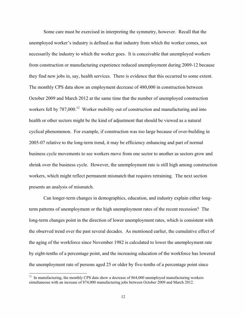
Some care must be exercised in interpreting the symmetry, however. Recall that the

unemployed worker’s industry is defined as that industry from which the worker comes, not

necessarily the industry to which the worker goes. It is conceivable that unemployed workers

from construction or manufacturing experience reduced unemployment during 2009-12 because

they find new jobs in, say, health services. There is evidence that this occurred to some extent.

The monthly CPS data show an employment decrease of 480,000 in construction between

October 2009 and March 2012 at the same time that the number of unemployed construction

workers fell by 787,000.12 Worker mobility out of construction and manufacturing and into

health or other sectors might be the kind of adjustment that should be viewed as a natural

cyclical phenomenon. For example, if construction was too large because of over-building in

2005-07 relative to the long-term trend, it may be efficiency enhancing and part of normal

business cycle movements to see workers move from one sector to another as sectors grow and

shrink over the business cycle. However, the unemployment rate is still high among construction

workers, which might reflect permanent mismatch that requires retraining. The next section

presents an analysis of mismatch.

Can longer-term changes in demographics, education, and industry explain either long-

term patterns of unemployment or the high unemployment rates of the recent recession? The

long-term changes point in the direction of lower unemployment rates, which is consistent with

the observed trend over the past several decades. As mentioned earlier, the cumulative effect of

the aging of the workforce since November 1982 is calculated to lower the unemployment rate

by eight-tenths of a percentage point, and the increasing education of the workforce has lowered

the unemployment rate of persons aged 25 or older by five-tenths of a percentage point since

12 In manufacturing, the monthly CPS data show a decrease of 864,000 unemployed manufacturing workers simultaneous with an increase of 874,000 manufacturing jobs between October 2009 and March 2012.

13

June 1992. Similar calculations show that the movement in the direction of services away from

manufacturing has lowered the experienced unemployment rate by two-tenths of a percentage

point since February 2001.

None of these trends in demographics, education, nor industrial composition can explain

the sharp rise in unemployment over the 2007-2009 recession. The composition changes in

Table 1 are all consistent with lower unemployment rates (all else equal) in all sub-periods. The

economy is continuing to move toward demographic groups and industries with lower

unemployment rates, not higher ones.

Although recessions may be idiosyncratic in terms of which demographic groups or

industries lead the increase in the unemployment rate, there is no evidence in the simple time

series that suggests fundamental structural change. Specifically, the economy’s industrial and

demographic mix has not changed in a way that explains higher unemployment rates that have

persisted over the past few years. The changing composition of the economy, either industrial or

demographic, has not led to permanently higher rates of unemployment.13 It is possible that

another kind of structural shift has occurred, such that workers’ skills do not match those

demanded by the economy. That possibility is considered in the next section.

II. Mismatch Unemployment

Mismatch occurs when the vacancies available in an industry, occupation, or location do

not match the skills of the workers available.14 When there is mismatch, a change in the skill

composition of the workforce (or skill requirements of the jobs available) is required to reduce

unemployment. Mismatch can take a number of forms. For example, the jobs may be in San

13 This is also the conclusion of Hoynes, Miller, and Schaller (2012) and Rothstein (2012). 14 The logic of our discussion traces its roots back to a suggestion made by Mincer (1966).

14

Francisco but the workers may be in Washington, D.C., or there may be many unemployed

construction workers but few vacancies in construction while there are few unemployed health

care workers but many vacancies in health care. If instead there are many vacancies in

construction and many unemployed workers in construction, while there are few vacancies in

health care and few unemployed heath care workers, the situation is not one of mismatch. In the

latter situation, changing the skill mix of the workforce would not remedy the problem.

A labor market mismatch seems to connote a structural problem, but the problem is not

necessarily structural if the situation is temporary. Structural shifts are usually taken to mean

changes that are permanent or at least long lasting enough so that retraining or changes in the

industrial composition would be appropriate and economically justified. But if the mismatch is

temporary, then major reinvestment, either in skills or in physical capital, is unwarranted. This is

particularly true if the situation is predictable. For example, construction workers know that

their industry is more cyclically sensitive than the health industry. There exists evidence of a

cyclical premium paid in construction relative to more stable industries and those in construction

may plan for alternative activity during slow periods.15

Conversely, structural problems may exist, even if there is no mismatch. It is possible

that every industry has the same ratio of unemployed workers to vacancies but that the ratio is

high and permanent, relative to past levels, perhaps because of labor market restrictions that

make employment costly. Fundamental changes in the economy, perhaps in government policy,

might be required to remedy the high unemployment situation, even in the absence of labor

market mismatch. Mismatch problems are not easily remedied by central banks, which cannot

bring about fundamental changes in the skill and/or industrial structure.

15 See Abowd and Ashenfelter (1981).

15

Defining Mismatch

What is a mismatch? If Ui is defined as the number of unemployed in industry,

occupation, or location i, and Vi is defined as the number of vacancies in the same industry,

occupation, or location i, then one possibility is to define mismatch as Ui ≠Vi. Although this is a

possibility, as an empirical matter, it would mean that the economy is always in a state of

mismatch because the measured number of unemployed workers always exceeds the measured

number of vacancies at the aggregate level.

There are also conceptual reasons why Ui = Vi is not the appropriate benchmark. First, if

the social cost of a worker waiting to find a job is lower than the cost of leaving a job unfilled, it

would be efficient to have workers queue for jobs rather than jobs queue for workers.16

Additionally, there may be measurement issues. As an empirical matter, vacancies are measured

as job openings on the last day of the month whereas unemployed workers are measured as of

the week of the 12th of the month. This difference in reference periods suggests that aggregate

unemployment should exceed aggregate vacancies.

Consequently, mismatch is defined as a situation where industries differ in their ratio of

unemployed to vacancies (we describe our mismatch index in terms of industries; we could also

use occupations or locations). Define λ as the ratio of total unemployed to total vacancies for the

economy as a whole. The policy community views λ with considerable interest and the BLS

updates its time series of every month (see chart 1 at

http://www.bls.gov/web/jolts/jlt_labstatgraphs.pdf). A balanced economy is one in which each

industry i has Ui/Vi = λ. An economy has mismatch when industry specific unemployment Ui

16 Optimal inventory policy implies that the inventories are seen as the side of the market that has the lowest cost of waiting.

16

deviates from that which would be predicted given the industry specific vacancy rate Vi and the

aggregate unemployment-to-vacancy ratio λ. For example, in the top graph of Figure 3, there are

two industries and the ratio of Ui / Vi in each of the two industries is equal to λ. The line

connecting the (U,V) points for each industry in the top graph of Figure 3 is the aggregate labor

market tightness line, and connects the origin and the aggregate (U,V) point. This aggregate

tightness line has a slope of (1/). In the bottom panel of Figure 3, the aggregate tightness line is

the same as in the upper panel, but now there is mismatch across the two industries, with one

industry having an excess of unemployed workers and the other having an excess of vacancies

relative to the economy-wide pattern. The horizontal dashed lines in the bottom panel of Figure

3 measure the number of unemployed persons that would need to be reallocated across industries

to result in Ui/Vi = λ for all i.

The index of mismatch that used here is a distance measure, defined as

(3) ∑ | |

where λ≡U/V, ≡ ∑ , and ≡ ∑ . In equation (3), the numerator measures the horizontal

distance of each industry, occupation, or location from the aggregate tightness line. The absolute

values ensures that the horizontal distance is positive for each i. Division by 2 is necessary to

avoid double-counting, and dividing by aggregate unemployment makes M the proportion of

unemployed workers who would need to be moved to make Ui/Vi = λ for all i.17 The logic of the

mismatch index M is that if each mismatch carries with it a constant social cost (e.g., retraining

17 Manipulation of this index results in ∑ . The idea for an index of this sort dates back at

least to Mincer (1966) and has been used by Jackman and Roper (1987), and more recently Dickens (2011) and Sahin et.al. (2011). Sahin et.al. use a matching function and an aggregate job-finding rate to determine the number of hires lost due to mismatch and the resulting counterfactual unemployment rate.

17

cost per worker), then a linear index in the number of mismatches captures the total social cost.

The numerator of (3) is proportional to the social cost of mismatch because it merely adds up the

total number of mismatches in the economy.

This mismatch index ranges from zero to one.18 It equals zero when every industry is in

perfect alignment so that the ratio of unemployed to vacancies in each industry equals the ratio of

unemployed to vacancies at the aggregate level. It equals one when industries are in complete

misalignment so that half the industries (weighted by size) have zero vacancies and positive

unemployment and half the industries have zero unemployed and positive vacancies.

The index has the property that increasing unemployment by a scalar in each industry

leaves M unchanged. This is a desirable property because increasing the number of unemployed

during a recession in a completely neutral way should not be interpreted as an increase in

mismatch.19

Measuring Mismatch

Measuring mismatch requires estimates of Ui and Vi. These are available for industries,

occupations, and locations. In this paper, we present estimates of industry mismatch and

occupational mismatch. Dickens (2011) and Sahin et.al. (2011) both find that geographical

mismatch is negligible. Consequently, no estimates of geographical mismatch are presented.

18 This is shown in the appendix, available on request. 19 Aggregate unemployment and vacancy data determine the location on the Beveridge curve at any particular point in time. Recessions are characterized by increasing (the aggregate U-to-V ratio) as the economy moves down and right along the Beveridge curve. However, it is the underlying Ui and Vi, rather than the aggregate U and V, that drives both M and λ. If shocks are highly idiosyncratic across industries, then M and λ will tend to be positively correlated because a big positive shock in any particular Ui (or big negative shock to Vi) will raise M and increase λ. However, if shocks are close to proportional across industries, then M and would not be correlated because would move even though M does not. Thus it is possible for an economy to move along the Beveridge curve with either an increase or no change to the mismatch index M.

18

To measure industrial mismatch, we use vacancy data by industry from the Job Openings

and Labor Turnover Survey (JOLTS) and unemployment data by industry from the Current

Population Survey (CPS). The data are publicly available data from the BLS website.20 The

JOLTS data begin in December 2000. Monthly data from January 2001 to December 2011 are

used to estimate industrial mismatch.

Vacancy data by occupation are obtained from the Help Wanted Online Index (HWOL)

and unemployment data by occupation are taken from the CPS to measure occupational

mismatch.21 The HWOL data begin in May 2005 and occupational mismatch is calculated over

the period from May 2005 to December 2011.22

Industrial Mismatch

Figure 4 presents the year-specific vacancy-unemployment plots. Time series graphs of

the monthly levels of industry unemployment and vacancies from January 2001 to December 20 Seasonally adjusted vacancy data is available for 12 industries and non-seasonally adjusted vacancy data is available for 24 industries (www.bls.gov/jlt). Non-seasonally adjusted unemployment data is available for 17 industries (www.bls.gov/cps). We download the non-seasonally adjusted JOLTS and CPS industry data and seasonally adjust all series using SAS proc X11. A 1:1 correspondence for JOLTS and CPS industries is possible for the following 12 industries: Mining, Construction, Manufacturing (we aggregated durable and nondurable manufacturing), Wholesale & Retail, Transportation & Utilities, Information, Financial Activities, Professional & Business Services, Education & Health Services, Leisure & Hospitality, Other Services, and Government. 21 We thank June Shelp of the Conference Board for providing us with the seasonally adjusted time series of HWOL data by occupation. The Conference Board reports vacancies by occupation in Table 7 of their monthly press release (see, for example, http://www.conference-board.org/data/helpwantedonline.cfm). The seasonally adjusted HWOL vacancy data is available for 22 occupations. Non-seasonally adjusted unemployment data by occupation is available (at www.bls.gov/cps) for 9 occupations and for persons with no previous occupation. We seasonally adjust the unemployment by occupation data and define the experienced unemployed. The experienced unemployed (measured by occupation) averages 91 percent of the total unemployed during the 2001 – 2011 time period. The HWOL and CPS occupational series correspond for the following 9 occupations: Management, Business and Financial Operations; Professional; Services; Sales; Office and Administrative Support; Construction; Installation and Maintenance; Production; and Transportation & Material Moving. 22 A natural question is how the JOLTS and the HWOL compare in measuring vacancies. The correlation of these two seasonally adjusted monthly series is 0.57. The JOLTS series is higher than the HWOL series prior to the recession (by an average of 423 thousand per month during the May 2005 – January 2008 time period), and the JOLTS series is lower than the HWOL series during and after the recession (by an average of 693 thousand during the February 2008 through December 2011 time period). The JOLTS and HWOL are graphed in Figure 1 of Sahin et.al. (2011).

19

2011 are presented in an appendix.23 The upper-left graph of Figure 4 is the annual averages of

Ui and Vi for 2006. The line that runs through the origin is the aggregate labor market tightness

line, the slope of which is 1/. In 2006, there are four industries characterized by relatively low

unemployment and relatively high vacancies: professional and business services, education and

health services, government, and financial activities. There are also four industries characterized

by relatively high unemployment and relatively low vacancies: wholesale and retail trade, leisure

and hospitality, manufacturing, and construction. The other four unlabeled industries (mining,

transportation and utilities, information, and other services) are small industries and are clustered

around the origin.

Obvious in Figure 4 is the changing slope of the aggregate tightness line as the recession

hits. The slope of this line is 0.741 in 2007, .479 in 2008, and .197 in 2009. (These statistics

correspond to the well-known U/V ratio of 1.4 in 2007, 2.1 in 2008, and 5.1 in 2009). Note that

the four industries to the left of the aggregate tightness line in 2006 are to the left in every year,

and the four industries to the right of the aggregate tightness line in 2006 are to the right in every

year.

Figure 5 shows how the mismatch index, M, varies over time. Mismatch is highly pro-

cyclic, rising during the 2001 recession, falling during the expansion of the mid-2000s, rising

through most of the 2007-2009 recession, and then falling since the end of the recession in June

2009. The lowest level of the industrial mismatch index M is .144 in January 2007, when 14.4

percent of unemployed workers would need to be reallocated across industries to put all

industries on the aggregate tightness line. The highest level of the index is .320 in April 2009.24

23 The appendix is available on request. 24 There is nothing mechanical about the increase in M during recessions. M goes up because certain industries tend to experience large increases in the number of unemployed during recession. This changes the aggregate ratio of

20

Which industries are responsible for the increase in the index during the recession? The

top panel of Table 2 presents descriptive statistics describing the rise of the index from .188 in

December 2007 to .288 in June 2009.25 At the beginning of the recession (December 2007), the

construction industry and the education and health services industry were the furthest away (size

weighted) from the aggregate tightness line. However, the manufacturing industry is responsible

for one-third of the recessionary increase in the index, with Education and Health Services,

Government, and Construction being responsible for a combined 63 percent of the recessionary

increase in the index. As seen in the bottom panel of Table 2, these same four industries are

responsible for most of the decline in the industrial mismatch index between June 2009 and

November 2011. Most of the action results not from the vacancy side, but from the tripling in

unemployment in manufacturing and construction. This had the effect of putting these two

industries far off the V/U line and also of bringing that line down. Because of the latter,

education and health services and government move farther away from the line, not because they

had such large increases in unemployment, but because their increases in unemployment and

decreases in vacancies did not match those of the economy as a whole. As a result, those

industries are further from the V/U line during the recession than they are in 2007. It is still true,

however, that the level of unemployment went up in every industry so that the number of

unemployed exceeded the number of vacancies in every industry in 2009-2011.

Most important is that the industrial mismatch index in late 2011 is at the same level as

before the 2007-2009 recession. Even though the average level of unemployment in 2011 is

almost double the average level of unemployment in 2007, the percent of unemployed persons

unemployed to vacancies, but the distance of specific industries from the aggregate line increases because the shocks are not balanced across industries. 25 We use 3-quarter moving averages of the monthly industrial mismatch index in Figure 5 to smooth large month-to-month movements. Shares and unemployment rates by industry can be inferred from Figures 1 and 2.

21

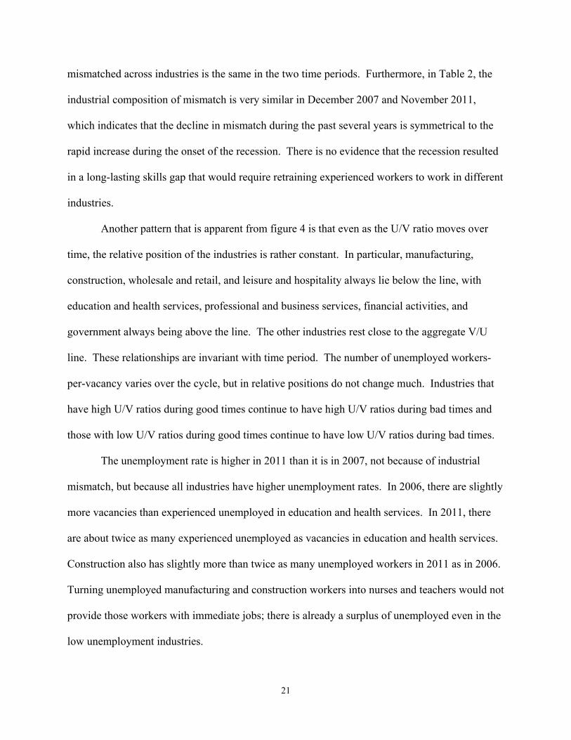
mismatched across industries is the same in the two time periods. Furthermore, in Table 2, the

industrial composition of mismatch is very similar in December 2007 and November 2011,

which indicates that the decline in mismatch during the past several years is symmetrical to the

rapid increase during the onset of the recession. There is no evidence that the recession resulted

in a long-lasting skills gap that would require retraining experienced workers to work in different

industries.

Another pattern that is apparent from figure 4 is that even as the U/V ratio moves over

time, the relative position of the industries is rather constant. In particular, manufacturing,

construction, wholesale and retail, and leisure and hospitality always lie below the line, with

education and health services, professional and business services, financial activities, and

government always being above the line. The other industries rest close to the aggregate V/U

line. These relationships are invariant with time period. The number of unemployed workers-

per-vacancy varies over the cycle, but in relative positions do not change much. Industries that

have high U/V ratios during good times continue to have high U/V ratios during bad times and

those with low U/V ratios during good times continue to have low U/V ratios during bad times.

The unemployment rate is higher in 2011 than it is in 2007, not because of industrial

mismatch, but because all industries have higher unemployment rates. In 2006, there are slightly

more vacancies than experienced unemployed in education and health services. In 2011, there

are about twice as many experienced unemployed as vacancies in education and health services.

Construction also has slightly more than twice as many unemployed workers in 2011 as in 2006.

Turning unemployed manufacturing and construction workers into nurses and teachers would not

provide those workers with immediate jobs; there is already a surplus of unemployed even in the

low unemployment industries.

22

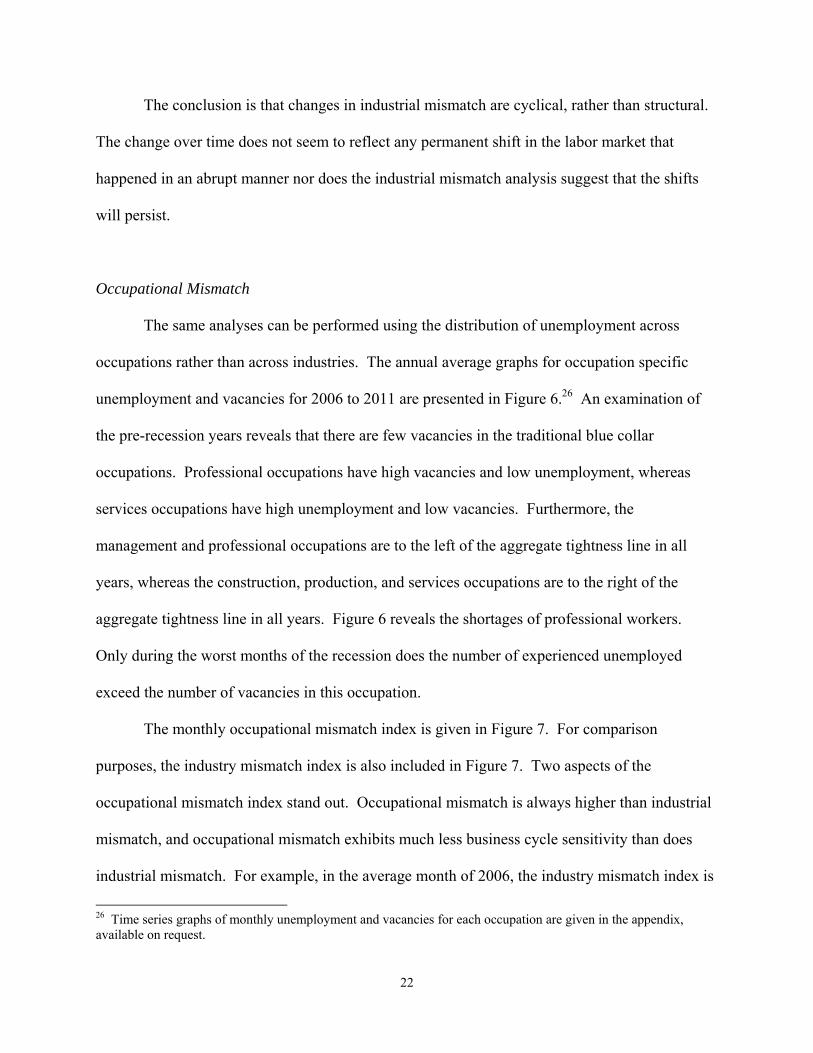
The conclusion is that changes in industrial mismatch are cyclical, rather than structural.

The change over time does not seem to reflect any permanent shift in the labor market that

happened in an abrupt manner nor does the industrial mismatch analysis suggest that the shifts

will persist.

Occupational Mismatch

The same analyses can be performed using the distribution of unemployment across

occupations rather than across industries. The annual average graphs for occupation specific

unemployment and vacancies for 2006 to 2011 are presented in Figure 6.26 An examination of

the pre-recession years reveals that there are few vacancies in the traditional blue collar

occupations. Professional occupations have high vacancies and low unemployment, whereas

services occupations have high unemployment and low vacancies. Furthermore, the

management and professional occupations are to the left of the aggregate tightness line in all

years, whereas the construction, production, and services occupations are to the right of the

aggregate tightness line in all years. Figure 6 reveals the shortages of professional workers.

Only during the worst months of the recession does the number of experienced unemployed

exceed the number of vacancies in this occupation.

The monthly occupational mismatch index is given in Figure 7. For comparison

purposes, the industry mismatch index is also included in Figure 7. Two aspects of the

occupational mismatch index stand out. Occupational mismatch is always higher than industrial

mismatch, and occupational mismatch exhibits much less business cycle sensitivity than does

industrial mismatch. For example, in the average month of 2006, the industry mismatch index is

26 Time series graphs of monthly unemployment and vacancies for each occupation are given in the appendix, available on request.

23

about half that of the occupation mismatch index. There are two immediate explanations for the

higher level of occupational mismatch. The first is that there are shortages of the traditional

white collar occupations (management and professional) that are not captured in the industry

data since managers and professional workers work in all industries. The second possible

explanation is measurement related. It is certainly possible that vacancies for the high-skilled

occupations are formally advertised and thus captured by the HWOL and the JOLTS, whereas

vacancies for the low skilled occupations might be informally advertised and missed in the data.

Whatever the cause, there appears to be a substantial amount of occupational mismatch relative

to industrial mismatch. But most important is that as with the industry data, the occupational

mismatch index has already returned to (actually fallen below) its pre-recession level. There

seems to be nothing structural, defined as permanent, about even the minor increases in

occupational mismatch that occurred during the last recession.

Mismatch Reversion and Policy

Defined either in terms of industry or occupation, the reversion of M to levels that

prevailed in the pre-recession period does not imply that all is well and that retraining would not

help alleviate the situation. A more fluid labor market, where individuals could move from one

sector to another sector more readily, or one in which workers were more aligned with vacancies,

could bring about a lower long run level of M. Although the current level of M approaches those

levels seen in the pre-recession mid-2000s, it is conceivable that the level of M could be even

lower. With respect to occupational mismatch, movement of workers from services into the

professional category, if it could be done, would have lowered M even in the robust labor market

24

of 2006. Similarly, in that same year a smooth conversion of construction workers into

education and health workers would have lowered M.

The fact that M appears to be retracing its footsteps does not imply that retraining is not

beneficial. It implies only that the increase in mismatch seen during the recent (and prior

recession) is a temporary phenomenon that tends to retreat as the economy recovers.

Summary of Mismatch

Increasing industrial mismatch is an important part of the recent recession, but the

increase was a transitory phenomenon. The industrial mismatch and occupational mismatch

indices have reverted to the pre-recessionary levels that prevailed in 2006 and 2007. Many who

believe that the labor market has fundamentally changed suggest that this is a consequence of

jobs being unavailable for certain kinds of workers, most often those who were employed in

manufacturing and construction. However, the analysis presented here shows that the most

recent recession has not resulted in any long-run increase in mismatch across industries or

occupations. The unemployment rate is higher now, not because skills available are less in line

with skills desired than they were in the past, but because unemployment rates are higher

generally across all industries and occupations.

III. Other Possible Structural Shifts

The evidence from the previous two sections makes clear that the high unemployment

rates that are prevalent today and that have persisted for the past few years are not a result of

changes in the occupation or industrial structure or of changes in relative demand and supply by

sector or demographic group. Although it is true that the different sectors of the economy have

25

not been hit uniformly by the recession, the lack of uniformity in increasing unemployment rates

by industry has been matched by similar asymmetry in the decreasing unemployment rates thus

far. Furthermore, the historic pattern of more cyclic sensitivity in certain industries like

construction and manufacturing is repeated in the recent recession.

The continuing high unemployment rate at the national level reflects elevated

unemployment in general and seems to be consistent with cyclic phenomena. But

unemployment rates are still elevated significantly and there remains the possibility that the

increase is long-lasting and in this sense, structural.

Making Work Less Valuable

Higher unemployment rates in all industries and many demographic groups might result

if wages are distorted as suggested by Mulligan (2012). Mulligan argues that the decrease in

employment that occurred during the recession was a result of a higher implicit tax on work,

which he defines as “the extra taxes paid, and subsidies foregone, as the result of working,

expressed as a ratio to the income from working.” He documents large increases in this ratio that

occurred as a result of stimulus legislation, which lengthened the insured unemployment period,

increased food stamp subsidies, and initiated programs related to health and mortgage assistance

that required low income status, among others. Mulligan concludes that most of the decline in

work hours that resulted during the recession was a result of government-induced distortions that

reduced the value of work.

If one accepts the Mulligan view, then the forecast for the future depends on forecasts

about fiscal policy. If transfers revert to previous levels, presumably labor supply behavior will

26

return to its pre-2009 pattern. Instead, if at least some of the changes are permanent or are

exacerbated by new legislation, we can expect the lower levels of work hours to persist.

Rothstein (2012) disputes the Mulligan view by providing evidence to show that wages

have fallen rather than risen during the relevant period. The Mulligan story is one of reduced

supply, which, Rothstein argues, should increase wages rather than decrease them. As a result,

Rothstein concludes that the shift is non-structural, at least insofar as structural is defined by

supply shifts.

It is certainly possible that the supply changes that Mulligan documents are real, but are

merely swamped by declines in demand that occurred during the recent recession. If so, wages

would fall in the short run, but unless the programs are eliminated (as some will be), supply

decreases may persist.

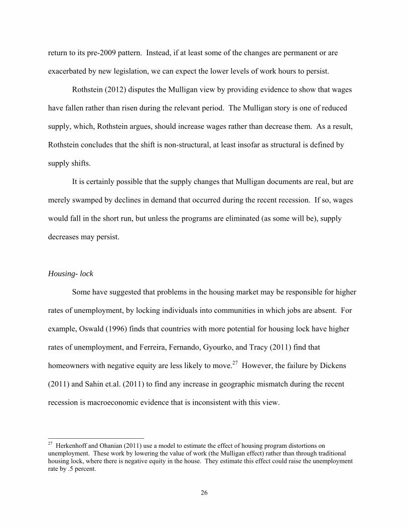
Housing- lock

Some have suggested that problems in the housing market may be responsible for higher

rates of unemployment, by locking individuals into communities in which jobs are absent. For

example, Oswald (1996) finds that countries with more potential for housing lock have higher

rates of unemployment, and Ferreira, Fernando, Gyourko, and Tracy (2011) find that

homeowners with negative equity are less likely to move.27 However, the failure by Dickens

(2011) and Sahin et.al. (2011) to find any increase in geographic mismatch during the recent

recession is macroeconomic evidence that is inconsistent with this view.

27 Herkenhoff and Ohanian (2011) use a model to estimate the effect of housing program distortions on unemployment. These work by lowering the value of work (the Mulligan effect) rather than through traditional housing lock, where there is negative equity in the house. They estimate this effect could raise the unemployment rate by .5 percent.

27

In addition, others, notably Farber (2012), have found that mobility data are inconsistent

with this view as well. Farber finds that although geographic mobility declined during the

recession for both owners and renters, the fall was primarily among renters, not owners. If the

housing-lock view were correct, one would expect the mobility of owners to fall relative to

renters, not the other way around. Thus, while the story is a plausible one, there seems to be

little support for it as an explanation of persistently high unemployment rates in the recent

recession.

Recent Shifts in the Beveridge Curve

The Beveridge curve plots the relationship over time between the unemployment rate on

the horizontal axis and the job openings rate on the vertical axis.28 The BLS publishes an

updated Beveridge curve every month (see chart 5 at

http://www.bls.gov/web/jolts/jlt_labstatgraphs.pdf), using unemployment rates from the CPS and

job openings rates from the JOLTS. The most recent Beveridge curve is displayed in Figure 8.

With minor exceptions, the curve is negatively sloped. As the economy slows, the

unemployment rate rises and the vacancy rate falls.

Figure 8 makes clear two phenomena. First, the points that characterize the recent

recession are far outside the range of prior experiences mapped out by the CPS and JOLTS data

between December 1990 and November 2007. Second, the return from peak unemployment

does not follow the same path as the journey to peak unemployment. In particular, the ratio of

vacancies-to-unemployment is higher when unemployment rates are falling than it is when

unemployment rates are rising. In the current recession and recovery, the Beveridge curve

28 The job openings rate is defined as the number of job openings divided by the sum of employment and job openings. See www.bls.gov/jlt for more information about JOLTS and job openings.

28

appears to have shifted out when comparing the October 2009 – May 2012 data to the December

2007 – June 2009 data.

Movements along the Beveridge curve are interpreted as cyclical movements in labor

demand, whereas shifts in the Beveridge curve up and to the right are typically interpreted as

structural shifts in unemployment, reflecting a reduced efficiency of matching workers to jobs.

The apparent outward shift in the Beveridge curve and the resulting increase in unemployment

may be consistent with a structural change that occurred after June 2009, but it is equally

consistent with the counter-clockwise dynamics observed in previous recessions and recoveries,

discussed in more detail in Valletta (2005) and Daly, Hobijn, Sahin, and Valletta (2012). The

intuition behind the dynamics is that the posting of vacancies increases before actual hiring

occurs, so there is a short-run increase in vacancies before unemployment declines. Extended

unemployment insurance benefits may contribute as the unemployed delay their return to work.

A decline in recruiting intensity by employers would also cause the Beveridge curve to

shift out. Recruiting intensity, as defined by Davis, Faberman, and Haltiwanger (2010), refers to

advertising, hiring standards, compensation packages, and other methods that employers use to

adjust the rate of hires per vacancy. Since vacancies are essentially costless for employers to

post on the internet, it is possible that employers have recently increased the number of vacancy

postings, some of which have low probabilities of being filled. Empirical evidence in support of

declining recruiting intensity during the recent recession is provided by Davis, Faberman, and

Haltiwanger (2012).29 Furthermore, relative to its pre-recessionary levels, recruiting intensity

29 The decline in recruiting intensity is important in explaining the Beveridge curve gap, which is defined as the higher unemployment rate at a given level of vacancies when comparing two Beveridge curves -- see Barnichon, Elsby, Hobijn, and Sahin, (2012). Barnichon et.al. show that the post-recessionary level of hires per vacancy is 38 percent less than predicted by the pre-recession data, and this low level of the vacancy yield more than fully explains the Beveridge curve gap. Barnichon et.al. also find that the construction industry contributes most to this Beveridge curve gap.

29

remains low in the 2009-2011 period. This is consistent with the counter-cyclical dynamics of

the Beveridge curve evident in previous recessions. Unemployment rates need to fall to their

pre-recessionary levels before any definitive conclusions can be drawn about a long-run shift in

the Beveridge curve. This is consistent with the view expressed by Bernanke (2012).

Employment and Hours Trends

Most of the analysis thus far has focused on unemployment rather than employment for

two reasons. First, the unemployment rate is often the focus of policymakers and the public.

Second, unemployment and employment are closely related, but changes show up more

dramatically (although this is a mere scaling issue) in unemployment. The seasonally adjusted

unemployment rate and the employment-to-population ratio have a correlation of -.87 during the

1975-2012 time period (see Figure 9). Still, it is useful to take a quick look at employment to

verify that nothing is happening there that is not mirrored in unemployment. As is evident in

Figure 9, the employment-to-population ratio trended up from 1975 until it peaked in 2000, and

like the unemployment rate, the employment-to-population ratio is cyclic. However, the

employment-to-population ratio has been essentially flat during the two most recent non-

recessionary time periods (rising by 0.6 percentage points from June 2003 to November 2007,

and neither rising nor falling during the October 2009 to March 2012 time period). Because the

denominator is either zero or close to zero for these recent time periods, it is not meaningful to

present the employment-to-population decompositions in a format similar to Table 1. For the

recent recessions, the decompositions of the employment-to-population ratios show similar

results as for the decomposition of the unemployment rate – the effects of composition shifts in

30

demographic characteristics are small in all sub-periods, and most of the explanatory power is in

changes in the employment-to-population ratio within demographic groups.30

The flattening of the employment-to-population ratio in the two most recent non-

recessionary time periods warrants further discussion. Measured from trough-to-peak, average

monthly net employment growth was 221,000 during the 1975 to 1980 time period, was 213,000

during the 1982-1990 time period, was 209,000 during the 1992-2000 time period, and was

135,000 during the 2003-2008 time period.31 This post-2000 slowdown in average monthly net

employment growth is also reflected in total hours worked, which grew by an annual average of

0.5% over the 2000-2007 period, compared to an annual average of 2.1% over the 1990-2000

period.32 At the same time, output has been rising, with real GDP at the end of 2007 being about

18% higher than it was in 2000. This means that changes in productivity account for the

increase in output. These trends are shown in Figure 10, using data from the BLS Major Sector

Productivity and Costs database.

Productivity growth seems to have substituted for hours over the 2000s decade. Firms

seem to be making do with fewer workers.33 In the short run, changes in the number of workers

demanded that are not coupled with declining wages show up as unemployment or as declining

labor force participation. It is too early to conclude that this reflects long run structural change.

Duration of Unemployment

30 It is not possible to decompose the cyclical movements in the employment-to-population ratio by industry, since the weights are the population shares (rather than labor force shares, as in Table 1), and industry is not defined for persons out of the labor force. 31 Expressed as an annual growth rate, measured from trough-to-peak, average net employment growth was 4.3% during the 1975 to 1980 time period, was 3.5% during the 1982-1990 time period, was 2.8% during the 1992-2000 time period, and was 1.5% during the 2003-2008 time period. 32 The hours tabulations use data from Table 6.9 of the Bureau of Economic Analysis’ national accounts. 33 See Lazear, Shaw and Stanton (2012) and Choi and Spletzer (2012).

31

One factor that differentiates this recession from others is that the duration of

unemployment has gone up dramatically (see Figure 11). In June 2012, those unemployed for 27

weeks or more accounted for 41.9% of the unemployed, and the percentage of long-term

unemployed has exceeded 40% for 31 consecutive months. Prior to the recent recession, the

highest proportion of long-term unemployed was 26%, which occurred in 1983. Rothstein

(2012) concludes that structural factors cannot explain the unprecedented rise in long-term

unemployment, arguing that the shifts that have occurred during the recent recession seem to be

temporary and cyclic. He claims that much of the increase in the proportion of long-term

unemployment can be explained by pre-existing trends and by the fact that the unemployment

rate is so high and has been for a long time. Still, it is troubling that the proportion of long-term

unemployment is so much higher than it was at the previous record level of 26% in 1983 when

unemployment rates were similarly high and for a similar amount of time.

It is possible to decompose the rise in duration in unemployment into that which results

from within-industry increases in unemployment duration and that which results from changing

weights of industries in the economy. The result is that the increase in unemployment durations

today relative to the 2001 recession are entirely due to changing within-industry durations.

Unemployment durations increased within every industry when comparing the 2007-2009

recession to the 2001 recession. Although construction has a larger share of unemployment in

the most recent recession than in 2001, this composition change has no effect on the

counterfactual unemployment durations.

There has been a shift in the reason for unemployment over the last three decades. When

unemployment was at its peak of 10.8% in November and December 1983, temporary job losers

accounted for 20.7% of the unemployed and permanent job losers accounted for 41.7% of the

32

unemployed.34 The seasonally unadjusted percent of unemployed who were unemployed for

more than 26 weeks was 19.6% in November and December 1983. At the unemployment peak

in October 2009, temporary job losers were 8.1% of the unemployed and permanent job losers

were 55.0% of the unemployed (and the seasonally unadjusted percent of unemployed who were

unemployed for more than 26 weeks was 38.0%). These statistics show that temporary layoffs

were more important in the early 1980s than now. But performing a decomposition analogous to

the one described above reveals that only a small amount of today’s higher unemployment

durations can be explained by the changing reason for unemployment. Instead, it is the higher

unemployment durations within almost every reason category that is driving today’s higher

unemployment durations.

IV. Conclusion

During the recent recession, unemployment rates rose to very high levels and then started

to retreat. At the same time, some industries, like construction, manufacturing, and retailing,

experienced disproportionately large increases in unemployment. But the patterns observed on

the way up were mirrored on the way down. Those industries that contributed much to the

increase in unemployment between 2007 and 2009 were the same that accounted for decreases in

unemployment since 2009.

The same is true for mismatch, which measures the difference between vacancies and

unemployed in an industry, occupation, or location. Industrial mismatch rose substantially

during the recent recession, but retreated just as quickly even as unemployment rates have

remained high. What happened on the way up happened symmetrically on the way down.

34 Additionally, 6.6% of the unemployed were job leavers, 21.2% were re-entrants, and 9.8% were new entrants.

33

Additionally, the current recession does not appear fundamentally different from prior

ones, except that it is worse. Indeed, the recovery has been weak overall. Since the end of the

recession in spring 2009, the economy has grown at a rate of 2.2% per year. The historical

relationship suggests that this relatively low GDP growth should result in 2.9 percent job growth

since the employment trough in 2009:Q4. This prediction is precisely the reality of 3.8 million

jobs created between 2009:Q4 and 2012:Q2. The problem is not that the labor market is under

performing; it is that the recovery has been very slow.

There are trends in the labor market, some of which began many decades ago. But the

trends cannot explain the sharp increase in unemployment that occurred between 2007 and 2009.

The timing does not fit and in most cases, the changes go in the wrong direction, implying lower

and less volatile unemployment rates, not higher ones.

One exception is that the ratio of long-term unemployed to total unemployed is higher

than it was in prior recessions including recessions with comparable unemployment rates.

However, this is not due to any observed structural change, but rather to the depth of the current

recession. Another possible exception is that there are more vacancies per unemployed person at

high levels of unemployment than was the case a couple of years ago. Whether this apparent

outward shift in the Beveridge curve is a permanent change cannot be known until

unemployment returns to normal levels.

The analysis in this paper and in others that we review do not provide any compelling

evidence that there have been changes in the structure of the labor market that are capable of

explaining the pattern of persistently high unemployment rates. The evidence points to primarily

cyclic factors.

34

References Aaronson, Daniel, Jonathan Davis, and Luojia Hu. 2012. “Explaining the Decline in the U.S. Labor Force Participation Rate.” Chicago Fed Letter #296, Federal Reserve Bank of Chicago. Aaronson, Daniel, Rissman, Ellen R., and Sullivan, Daniel G. 2004. “Can Sectoral Reallocation Explain the Jobless Recovery?” Economic Perspectives, Federal Reserve Bank of Chicago. Abowd, John, and Orley Ashenfelter. 1981. “Anticipated Unemployment, Temporary Layoffs, and Compensating Wage Differentials.” In Sherwin Rosen, ed., Studies in Labor Markets. Chicago: University of Chicago Press for the National Bureau of Economic Research, pp. 141–70. Abraham, Katharine, and Lawrence Katz. 1986. “Cyclical Unemployment: Sectoral Shifts or Aggregate Disturbances?” Journal of Political Economy 94, pp. 407–22. Barnichon, Regis, Michael Elsby, Bart Hobijn, and Ayşegül Şahin. 2012. “ Which Industries are Shifting the Beveridge Curve?” Monthly Labor Review, June 2012, Vol. 135, No. 6, pp. 25-37. Bentolila, Samuel and Giuseppe Bertola. 1990. “Firing Costs and Labour Demand: How Bad is Eurosclerosis?” The Review of Economic Studies, Vol. 57, No. 3 (Jul., 1990), pp. 381-402. Bernanke, Ben S. 2012. “Recent Developments in the Labor Market” Remarks to the National Association for Business Economics, Washington, D.C., March 26, 2012, http://www.federalreserve.gov/newsevents/speech/bernanke20120326a.pdf. Brainard, Lael, and David Cutler. 1993. “Sectoral Shifts and Cyclical Unemployment.” Quarterly Journal of Economics, pp. 219–243. Charles, Kerwin Kofi, Erik Hurst, and Matthew J. Notowidigdo. 2012. “Manufacturing Busts, Housing Booms, and Declining Employment: A Structural Explanation.” Unpublished paper, University of Chicago. Available at http://faculty.chicagobooth.edu/erik.hurst/research/charles_hurst_noto_manufacturing.pdf Choi, Eleanor J. and James R. Spletzer. 2012. “ The declining average size of establishments: evidence and explanations.” Monthly Labor Review, March 2012, Vol. 135, No. 3, pp. 50-65. Clague, Ewan. 1935. “The Problem of Unemployment and the Changing Structure of Industry,” Journal of the American Statistical Association, vol. 30, no. 189, Supplement, pp. 209-14. Daly, Mary, Bart Hobijn, and Rob Valletta. 2011. “The Recent Evolution of the Natural Rate of Unemployment.” IZA Discussion Paper #5832, http://ftp.iza.org/dp5832.pdf.

35

Daly, Mary C., Bart Hobijn, Ayşegül Şahin, and Robert G. Valletta. 2012. “A Search and Matching Approach to Labor Markets: Is the Natural Rate of Unemployment Rising?” Forthcoming, Journal of Economic Perspectives. Davis, Steven J., R. Jason Faberman, and John C. Haltiwanger. 2010. “The Establishment-Level Behavior of Vacancies and Hiring.” NBER Working Paper No. 16265. Davis, Steven J., R. Jason Faberman, and John C. Haltiwanger. 2012. “Recruiting Intensity during and after the Great Recession: National and Industry Evidence.” American Economic Review Papers and Proceedings, 102(3), pp. 584-588. Dickens, William T. 2011. “Has the Recession Increased the NAIRU?” Unpublished paper, Brookings Institution. http://www.brookings.edu/~/media/research/files/papers/2011/6/ 29%20recession%20nairu%20dickens/0629_recession_nairu_dickens.pdf. Elsby, Michael, Bart Hobijn, and Ayşegül Şahin. 2010. “The Labor Market in the Great Recession.” Brookings Papers on Economic Activity, pp. 1-48. Elsby, Michael, Bart Hobijn, Ayşegül Şahin, and Robert G. Valletta. 2011. “The Labor Market in the Great Recession: An Update” Brookings Papers on Economic Activity, pp. 353-371. Estevao, Marcello and Tsounta Evridiki. 2011. “Has the Great Recession Raised U.S. Structural Unemployment?” IMF Working Paper #11/105. http://www.imf.org/external/pubs/ft/wp/2011/wp11105.pdf. Farber, Henry S. 2012. “Unemployment in the Great Recession: Did the Housing Market Crisis Prevent the Unemployed from Moving to Take Jobs?” American Economic Review Papers and Proceedings, 102(3), pp. 520-525. Ferreira, Fernando, Joseph Gyourko, and Joseph Tracy. 2011. “Housing Busts and Household Mobility: An Update.” NBER Working Paper #17405. Groshen, Erica and Simon Potter. 2003. “Has Structural Change Contributed to a Jobless Recovery?” Federal Reserve Bank of New York, Current Issues in Economics and Finance, Vol. 9, Number 8. Herkenhoff, Kyle F. and Lee E. Ohanian. 2011. “Labor Market Dysfunction During the Great Recession.” NBER Working Paper #17313. Hoynes, Hilary W., Douglas L. Miller, and Jessamyn Schaller. 2012. “Who Suffers During Recessions.” NBER Working Paper #17951. Jackman, R. and S. Roper. 1987. “Structural Unemployment.” Oxford Bulletin of Economics and Statistics. 49(1), pp. 9-36.

36

Kocherlakota, Narayana. 2010. “Inside the FOMC.” Available at http://www.minneapolisfed.org/news_events/pres/kocherlakota_speech_08172010.pdf. Lazear, Edward P. 1990. “Job Security Provisions and Employment.” The Quarterly Journal of Economics, Vol. 105, No. 3 (Aug., 1990), pp. 699-726. Lazear, Edward P., Kathryn L. Shaw, and Christopher T. Stanton. 2012. “The Value of Bosses.” Unpublished working paper, Stanford University. Lilien, David. 1982. “Sectoral Shifts and Cyclical Unemployment.” Journal of Political Economy 90, pp. 777–793. Loungani, Prakash, Mark Rush, and William Tave. 1990. “Stock Market Dispersion and Unemployment.” Journal of Monetary Economics (June) pp. 367–388. Mincer, Jacob. 1966. “Comment on ‘The Concept of Job Vacancies in a Dynamic Theory of the Labor Market’” in “The Measurement and Interpretation of Job Vacancies,” Columbia University Press. Available at http://www.nber.org/books/unkn66-2. Mulligan, Casey B. 2012. The Redistribution Recession. Forthcoming, Oxford University Press, 2012. Oswald, Andrew. 1996. “A Conjecture on the Explanation for High Unemployment in the Industrialized Nations: Part I,” University Of Warwick Economic Research Paper #475, available at http://wrap.warwick.ac.uk/1664/1/WRAP_Oswald_475_twerp_475.pdf. Rissman, Ellen R. 2009. “Employment growth: Cyclical movements or structural change?” Economic Perspectives, Federal Reserve Bank of Chicago. Romer, Christina D. 2011. “The Continuing Unemployment Crisis: Causes, Cures, and Questions for Further Study.” Speech given at Washington University, available at http://elsa.berkeley.edu/~cromer/Washington%20University%20final.pdf. Rothstein, Jesse. 2012. “The Labor Market Four Years Into the Crisis: Assessing Structural Explanations.” NBER Working Paper #17966. Sahin, Ayşegül, Joseph Song, Giorgio Topa, and Giovanni L. Violante. 2011 (July). “Measuring Mismatch in the U.S. Labor Market.” Unpublished Paper, Federal Reserve Bank of New York, available at http://nyfedeconomists.org/topa/USmismatch_v14.pdf. Valletta, Robert G. 2005. “Why Has the U.S. Beveridge Curve Shifted Back? New Evidence Using Regional Data.” Federal Reserve Bank of San Francisco Working Paper #2005-25. Valletta, Rob and Katherine Kuang. 2010. “Is Structural Unemployment on the Rise?” FRBSF Economic Letter #2010-34.

37

Figure 1: Labor Force Shares by Gender, Age, Education, and Industry, 1975-2012 Source: CPS data downloaded from www.bls.gov/cps

35

45

55

65

1975

1977

1979

1981

1983

1985

1987

1989

1991

1993

1995

1997

1999

2001

2003

2005

2007

2009

2011

Labor Force Share Men Labor Force Share Women

0

25

50

75

1975

1977

1979

1981

1983

1985

1987

1989

1991

1993

1995

1997

1999

2001

2003

2005

2007

2009

2011

Labor Force Share 16‐19 Labor Force Share 20‐24

Labor Force Share 25‐54 Labor Force Share 55+

38

Figure 1 (continued)

Age 25+.

Experienced Labor Force. Mining and Information not in the graph.

0

10

20

30

40

1975

1977

1979

1981

1983

1985

1987

1989

1991

1993

1995

1997

1999

2001

2003

2005

2007

2009

2011

Labor Force Share < HS Labor Force Share HS Grads

Labor Force Share Some Coll Labor Force Share Coll Grads

0

5

10

15

20

25

1975

1977

1979

1981

1983

1985

1987

1989

1991

1993

1995

1997

1999

2001

2003

2005

2007

2009

2011

Construction Manufacturing Wholesale TradeRetail Trade Transport & Utilities FinancialProf & Bus Services Educ & Health Services Leis & HospitalityOther Services Government

39

Figure 2: Unemployment Rates by Gender, Age, Education, and Industry, 1975-2012 Source: CPS data downloaded from www.bls.gov/cps

3

6

9

12

1975

1977

1979

1981

1983

1985

1987

1989

1991

1993

1995

1997

1999

2001

2003

2005

2007

2009

2011

U rate Men U rate Women U rate Total

0

10

20

30

1975

1977

1979

1981

1983

1985

1987

1989

1991

1993

1995

1997

1999

2001

2003

2005

2007

2009

2011

U rate 16‐19 U rate 20‐24 U rate 25‐54 U rate 55+ U rate Total

40

Figure 2 (continued)

Age 25+.

Experienced Labor Force. Mining and Information not in the graph.

0

6

12

18

1975

1977

1979

1981

1983

1985

1987

1989

1991

1993

1995

1997

1999

2001

2003

2005

2007

2009

2011

U Rate < HS U Rate HS Grads U Rate Some Coll

U Rate Coll Grads U Rate Total

0%

4%

8%

12%

16%

20%

1975

1977

1979

1981

1983

1985

1987

1989

1991

1993

1995

1997

1999

2001

2003

2005

2007

2009

2011

Construction Manufacturing Wholesale TradeRetail Trade Transport & Utilities FinancialProf & Bus Services Educ & Health Services Leis & HospitalityOther Services Government Total Experienced

41

Table 1: Unemployment Rate Decomposition by Gender, Age, Education, and Industry u = i [si*ui + si*ui] Dec 79 - Nov 82 - Jun 90 - Jun 92 - Feb 01 - Jun 03 - Nov 07 - Oct 09 - Nov 82 Jun 90 Jun 92 Feb 01 Jun 03 Nov 07 Oct 09 Mar 12

u 4.8 -5.5 2.6 -3.6 2.1 -1.6 5.3 -1.8

si*ui Male 69.0% 58.7% 64.0% 60.4% 62.1% 63.7% 64.4% 84.2% Female 30.4% 40.2% 37.0% 39.8% 38.4% 38.0% 35.9% 15.3% Sum 99.4% 98.9% 101.0% 100.2% 100.5% 101.7% 100.3% 99.5%

si*ui Male -1.6% 2.6% -0.5% 2.1% -0.5% -1.2% -0.3% 1.4% Female 1.6% -2.4% 0.5% -1.9% 0.5% 1.1% 0.3% -1.2% Sum 0.0% 0.2% 0.0% 0.2% 0.0% -0.1% 0.0% 0.2%

u 4.8 -5.5 2.6 -3.6 2.1 -1.6 5.3 -1.8

si*ui 16-19 14.0% 12.5% 19.7% 14.4% 13.5% 8.4% 8.7% 4.2% 20-24 19.9% 19.5% 13.8% 11.8% 14.7% 13.4% 13.8% 13.7% 25-54 62.6% 56.6% 60.0% 62.9% 64.3% 56.6% 66.1% 71.7% 55+ 7.9% 6.3% 11.4% 8.6% 10.9% 14.4% 13.4% 7.5% Sum 104.4% 94.9% 104.9% 97.7% 103.4% 92.8% 102.0% 97.1%

si*ui 16-19 -6.1% 5.2% -4.6% -0.6% -5.7% 3.9% -2.5% 3.3% 20-24 -1.1% 6.3% -1.7% 3.1% 0.6% 1.9% -0.7% -2.8% 25-54 3.3% -7.2% 2.5% 0.5% -2.4% 5.5% -0.6% 8.1% 55+ -0.5% 1.3% -0.2% -1.6% 3.1% -6.0% 1.4% -6.1% Sum -4.4% 5.6% -4.0% 1.4% -4.4% 5.3% -2.4% 2.5%

u -3.0 1.8 -1.3 4.9 -1.7

si*ui < HS 16.7% 10.7% 12.5% 14.2% 13.6% HS Grad 34.0% 34.1% 27.3% 39.0% 49.5% Some Coll 26.1% 31.9% 33.4% 31.0% 20.7% Coll Grad 15.0% 25.9% 22.5% 17.4% 10.1% Sum 91.8% 102.6% 95.7% 101.6% 93.9%

si*ui < HS 7.5% -1.6% 4.8% -0.5% 3.8% HS Grad 7.1% -2.3% 3.9% -1.4% 6.7% Some Coll -3.3% -0.5% -0.3% 0.2% -1.5% Coll Grad -3.3% 1.9% -3.3% 0.7% -3.5% Sum 8.0% -2.5% 5.1% -1.0% 5.5%

42

Table 1 (continued) Dec 79 - Nov 82 - Jun 90 - Jun 92 - Feb 01 - Jun 03 - Nov 07 - Oct 09 - Nov 82 Jun 90 Jun 92 Feb 01 Jun 03 Nov 07 Oct 09 Mar 12 u 1.9 -1.6 4.9 -1.9

si*ui Mining 0.3% 0.9% 1.0% 2.0% Construct 9.9% 11.5% 19.4% 21.5% Manufact 18.6% 19.9% 18.5% 30.9% Wholesal 3.9% 5.6% 2.3% 1.3% Retail 11.9% 13.1% 12.6% 8.2% Tran & Ut 4.6% 2.3% 4.0% 6.5% Informat 5.4% 4.2% 2.0% 1.0% Financial 3.6% 3.3% 5.7% 6.0% Prf & Bus 14.6% 19.5% 10.3% 6.6% Ed & Hlth 8.1% 7.3% 9.1% 1.2% Leisure 7.6% 2.9% 8.8% 11.8% Oth Serv 4.2% 4.5% 3.9% 2.0% Govt 9.1% 4.4% 3.9% -2.2% Sum 101.8% 99.4% 101.5% 96.8%

si*ui Mining 0.0% -0.2% 0.1% -0.8% Construct 0.6% -2.4% -1.7% 6.8% Manufact -4.8% 4.0% -1.5% 0.2% Wholesal 0.6% 1.0% -0.3% 0.1% Retail 0.8% 1.6% 0.0% -0.9% Tran & Ut -0.4% -1.1% -0.5% 0.1% Informat -0.3% 1.4% 0.0% 0.8% Financial -0.1% -0.3% -0.3% 0.1% Prf & Bus -0.2% -2.2% 0.3% -3.0% Ed & Hlth 1.1% -0.6% 0.8% -0.3% Leisure 0.2% -0.6% 1.1% -0.1% Oth Serv 0.5% -0.2% 0.1% 0.0% Govt 0.0% 0.1% 0.1% 0.0% Sum -2.0% 0.5% -1.8% 3.0%

Source: CPS data downloaded from www.bls.gov/cps Education results are for the population aged 25+. Industry results are for the Experienced Unemployed. Percentages may not add to 100% due to rounding.

43

Figure 3: Example of Mismatch

0

0

Vacancies

Unemployed

0

0

Vacancies

Unemployed

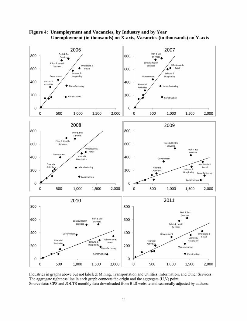
44

Figure 4: Unemployment and Vacancies, by Industry and by Year Unemployment (in thousands) on X-axis, Vacancies (in thousands) on Y-axis

Industries in graphs above but not labeled: Mining, Transportation and Utilities, Information, and Other Services. The aggregate tightness line in each graph connects the origin and the aggregate (U,V) point. Source data: CPS and JOLTS monthly data downloaded from BLS website and seasonally adjusted by authors.

Construction

Manufacturing

Wholesale & Retail

Financial Activities

Prof & Bus Services

Educ & Health Services

Leisure & HospitalityGovernment

0

200

400

600

800

0 500 1,000 1,500 2,000

2006

Construction

Manufacturing

Wholesale & Retail

Financial Activities

Prof & Bus Services

Educ & Health Services

Leisure & HospitalityGovernment

0

200

400

600

800

0 500 1,000 1,500 2,000

2007

Construction

Manufacturing

Wholesale & Retail

Financial Activities

Prof & Bus Services

Educ & Health Services

Leisure & Hospitality

Government

0

200

400

600

800

0 500 1,000 1,500 2,000

2008

Construction

Manufacturing

Wholesale & RetailFinancial 

Activities

Prof & Bus Services

Educ & Health Services

Leisure & Hospitality

Government

0

200

400

600

800

0 500 1,000 1,500 2,000

2009

Construction

Manufacturing

Wholesale & Retail

Financial Activities

Prof & Bus ServicesEduc & Health 

Services

Leisure & Hospitality

Government

0

200

400

600

800

0 500 1,000 1,500 2,000

2010

Construction

Manufacturing

Wholesale & Retail

Financial Activities

Prof & Bus Services

Educ & Health Services

Leisure & Hospitality

Government

0

200

400

600

800

0 500 1,000 1,500 2,000

2011

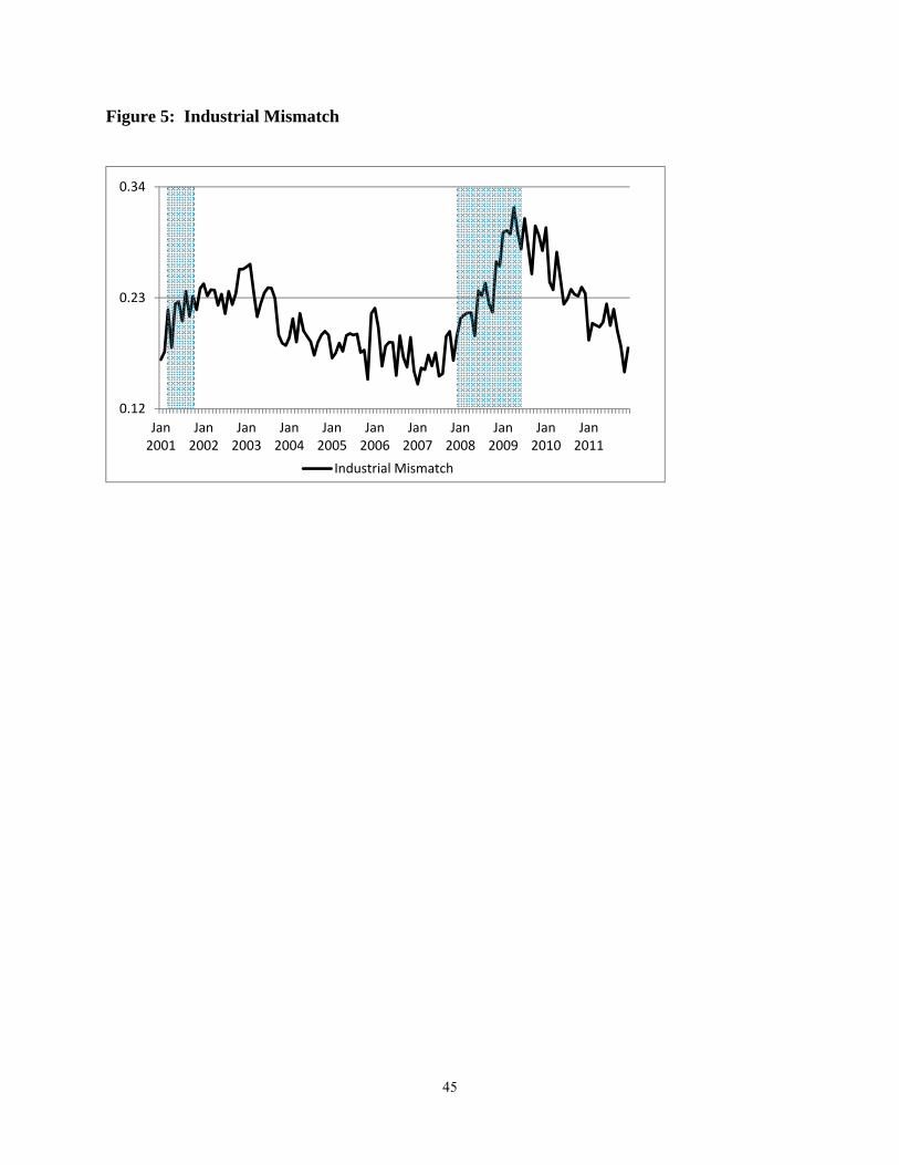
45

Figure 5: Industrial Mismatch

0.12

0.23

0.34

Jan 2001

Jan 2002

Jan 2003

Jan 2004

Jan 2005

Jan 2006

Jan 2007

Jan 2008

Jan 2009

Jan 2010

Jan 2011

Industrial Mismatch

46

Table 2: Industrial Mismatch (3 quarter moving average) December 2007 June 2009 Dec 07 – June 09 Mi Mi / M Mi Mi / M Mi Mi / M Mining 0.0004 0.2% 0.0027 0.9% 0.0023 2.3% Construction 0.0487 25.9% 0.0642 22.3% 0.0155 15.6% Manufacturing 0.0246 13.1% 0.0579 20.1% 0.0333 33.4% Wholesale & Retail 0.0121 6.5% 0.0002 0.1% -0.0119 -12.0% Transport & Utilities 0.0008 0.4% 0.0070 2.4% 0.0062 6.2% Information 0.0004 0.2% 0.0035 1.2% 0.0031 3.1% Financial Activities 0.0099 5.3% 0.0103 3.6% 0.0004 0.4% Prof & Bus Services 0.0290 15.4% 0.0245 8.5% -0.0045 -4.5% Educ & Health Serv 0.0411 21.8% 0.0685 23.8% 0.0273 27.5% Leisure & Hospitality 0.0073 3.9% 0.0085 3.0% 0.0012 1.2% Other Services 0.0025 1.3% 0.0091 3.2% 0.0066 6.6% Government 0.0111 5.9% 0.0313 10.9% 0.0202 20.3% Total 0.1882 100.0% 0.2878 100.0% 0.0995 100.0% June 2009 November 2011 June 09 – Nov 11 Mi Mi / M Mi Mi / M Mi Mi / M Mining 0.0027 0.9% 0.0010 0.6% -0.0017 1.5% Construction 0.0642 22.3% 0.0432 25.2% -0.0210 18.1% Manufacturing 0.0579 20.1% 0.0198 11.5% -0.0381 32.9% Wholesale & Retail 0.0002 0.1% 0.0112 6.5% 0.0110 -9.5% Transport & Utilities 0.0070 2.4% 0.0028 1.6% -0.0042 3.6% Information 0.0035 1.2% 0.0059 3.4% 0.0024 -2.1% Financial Activities 0.0103 3.6% 0.0040 2.3% -0.0063 5.5% Prof & Bus Services 0.0245 8.5% 0.0316 18.4% 0.0071 -6.1% Educ & Health Serv 0.0685 23.8% 0.0359 20.9% -0.0326 28.1% Leisure & Hospitality 0.0085 3.0% 0.0022 1.3% -0.0063 5.4% Other Services 0.0091 3.2% 0.0067 3.9% -0.0024 2.1% Government 0.0313 10.9% 0.0076 4.4% -0.0238 20.5% Total 0.2878 100.0% 0.1718 100.0% -0.1159 100.0%

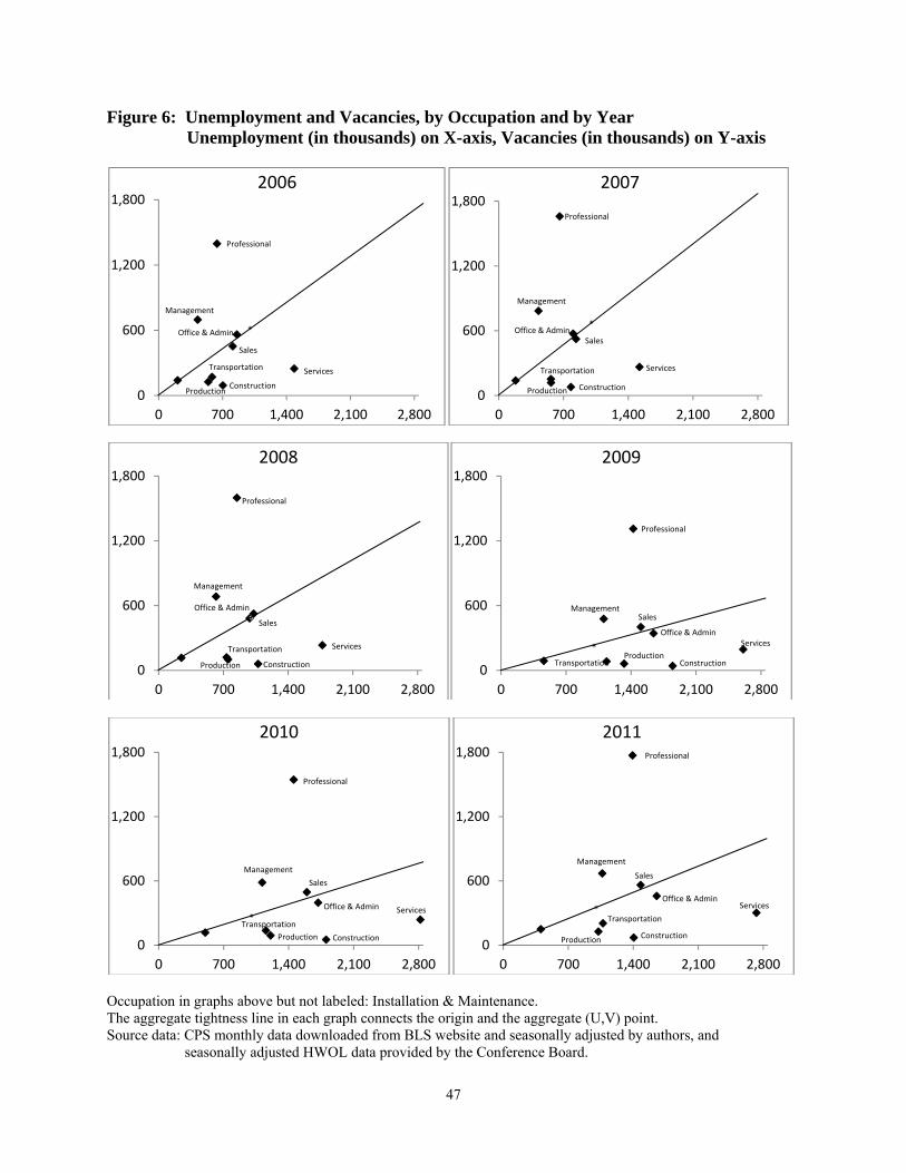
47

Figure 6: Unemployment and Vacancies, by Occupation and by Year Unemployment (in thousands) on X-axis, Vacancies (in thousands) on Y-axis

Occupation in graphs above but not labeled: Installation & Maintenance. The aggregate tightness line in each graph connects the origin and the aggregate (U,V) point. Source data: CPS monthly data downloaded from BLS website and seasonally adjusted by authors, and seasonally adjusted HWOL data provided by the Conference Board.

Management

Professional

Services

Sales

Office & Admin

ConstructionProduction

Transportation

0

600

1,200

1,800

0 700 1,400 2,100 2,800

2006

Management

Professional

Services

SalesOffice & Admin

ConstructionProduction

Transportation

0

600

1,200

1,800

0 700 1,400 2,100 2,800

2007

Management

Professional

Services

Sales

Office & Admin

ConstructionProduction

Transportation

0

600

1,200

1,800

0 700 1,400 2,100 2,800

2008

Management

Professional

Services

Sales

Office & Admin

ConstructionProduction

Transportation0

600

1,200

1,800

0 700 1,400 2,100 2,800

2009

Management

Professional

Services

Sales

Office & Admin

ConstructionProduction

Transportation

0

600

1,200

1,800

0 700 1,400 2,100 2,800

2010

Management

Professional

Services

Sales

Office & Admin

ConstructionProduction

Transportation

0

600

1,200

1,800

0 700 1,400 2,100 2,800

2011

48

Figure 7: Occupational and Industrial Mismatch

Figure 8: Beveridge Curve Source: http://www.bls.gov/web/jolts/jlt_labstatgraphs.pdf

0.12

0.23

0.34

0.45

January 2005

January 2006

January 2007

January 2008

January 2009

January 2010

January 2011

Industry Mismatch Occupation Mismatch

49

Figure 9: The Unemployment Rate and the Employment-to-Population Ratio Source: CPS data downloaded from www.bls.gov/cps

55

57

59

61

63

65

2

4

6

8

10

12

1975

1977

1979

1981

1983

1985

1987

1989

1991

1993

1995

1997

1999

2001

2003

2005

2007

2009

2011

Unemployment Rate (left axis) E/P Ratio (right axis)

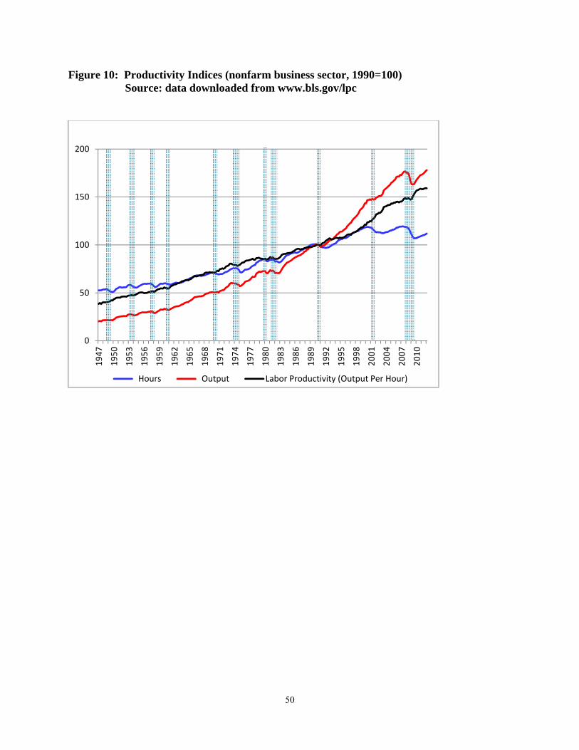
50

Figure 10: Productivity Indices (nonfarm business sector, 1990=100) Source: data downloaded from www.bls.gov/lpc

0

50

100

150

200

1947

1950

1953

1956

1959

1962

1965

1968

1971

1974

1977

1980

1983

1986

1989

1992

1995

1998

2001

2004

2007

2010

Hours Output Labor Productivity (Output Per Hour)

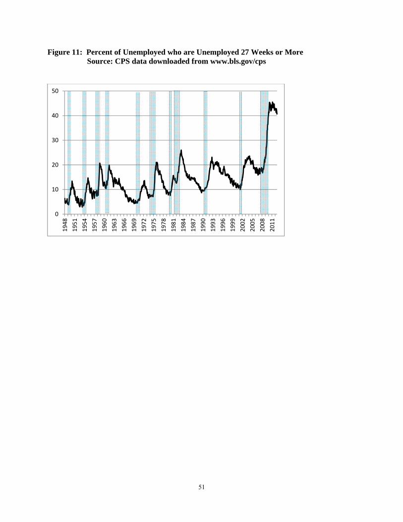
51

Figure 11: Percent of Unemployed who are Unemployed 27 Weeks or More Source: CPS data downloaded from www.bls.gov/cps

0

10

20

30

40

50

1948

1951

1954

1957

1960

1963

1966

1969

1972

1975

1978

1981

1984

1987

1990

1993

1996

1999

2002

2005

2008

2011