Stochastic Anal. Appl. Vol. 16, No. 4, 1998, (697-720)

Preprint Ser. No. 29, 1993, Math. Inst. Aarhus

The Uniform Mean-Square Ergodic Theoremfor Wide Sense Stationary Processes

GORAN PESKIR

It is shown that the uniform mean-square ergodic theorem holds for the family

of wide sense stationary sequences, as soon as the random process with orthogonal

increments, which corresponds to the orthogonal stochastic measure generated by

means of the spectral representation theorem, is of bounded variation and uniformly

continuous at zero in a mean-square sense. The converse statement is also shown to

be valid, whenever the process is sufficiently rich. The method of proof relies upon

the spectral representation theorem, integration by parts formula, and estimation of

the asymptotic behaviour of total variation of the underlying trigonometric functions.

The result extends and generalizes to provide the uniform mean-square ergodic

theorem for families of wide sense stationary processes.

1. Introduction

Let� f�n(t)gn2Z j t 2 T

�be a family of (wide sense) stationary sequences of complex

random variables defined on the probability space (;F ; P ) and indexed by the set T . Then

the mean-square ergodic theorem is known to be valid:

(1.1)1

n

n�1Xk=0

�k(t) ! Lt in L2(P )

as n!1 , for all t 2 T . The present paper is motivated by the following question: When does

the convergence in (1.1) hold uniformly over t 2 T ? In other words, when do we have:

(1.2) supt2T

��� 1n

n�1Xk=0

�k(t) � Lt

��� ! 0 in L2(P )

as n ! 1 ? It is the purpose of the paper to exhibit a solution for this problem, as well as to

motivate further research in this direction. We begin by recalling some historical facts.

This sort of problem originates in the papers of Glivenko [8] and Cantelli [3] who considered

the a.s. version of (1.2) in the i.i.d. case and proved the well-known Glivenko-Cantelli theorem.

Various generalizations and extensions of this result are shown to be of fundamental importance in

different fields ranging from Banach space theory to statistics. Here we do not wish to review the

more detailed history of this development, but will point out some of the fundamental results.

In the papers of Vapnik and Chervonenkis [18] and [19] the a.s. version of (1.2) is characterized

in the i.i.d. case in terms of random entropy numbers. This result is recently generalized and

extended into ergodic theory by obtaining uniform Birkhoff’s pointwise ergodic theorem (see [14]).

The extension happens to be valid for stationary ergodic (in the strict sense) sequences with an

AMS 1980 subject classifications. Primary 60F25, 60G10. Secondary 60B12, 60H05.Key words and phrases: Uniform ergodic theorem, (wide sense) stationary, the spectral representation theorem, orthogonal stochastic measure,random process with orthogonal increments, the Herglotz theorem, covariance function, spectral measure. goran@imf.au.dk

1

additional weak dependence structure involving a form of mixing. This research is moreover

indicated that the mixing property is important and can not be avoided. For this reason we see that

problem (1.2) goes far beyond the level where the entropy numbers could be of use.

Another approach towards the a.s. version of (1.2) in the i.i.d. case appeared in the papers

of Blum [2] and DeHardt [4]. They used the concept of metric entropy with bracketing (see [5]).

In this context they obtained by now the best known sufficient condition. Following this result, a

characterization of the a.s. version of (1.2) in the i.i.d. case is obtained in the paper of Hoffmann-

Jørgensen [9], which involves Blum-DeHardt’s theorem as a particular case. It is shown recently

that this result extends to the general stationary ergodic (in the strict sense) case (see [12]), as well

as to the case of general measurable dynamical systems (see [13]).

Somewhat different characterization of the a.s. version of (1.2) in the i.i.d. case is obtained in

the paper of Talagrand [17]. A close look into the proof indicates that this approach also requires

a form of mixing, and thus will be not taken into consideration here. To conclude the exposition

as stated above, we find it convenient to recall the papers [7], [10], [11] and [20].

The main novelty of the approach towards uniform ergodic theorem (1.2) taken in the present

paper relies upon the spectral representation theorem which is valid for (wide sense) stationary

sequences under consideration. It makes possible to investigate the uniform ergodic theorem (1.2)

in terms of the orthogonal stochastic measure which is associated with the underlying sequence by

means of the theorem, or equivalently, in terms of the random process with orthogonal increments

which corresponds to the measure. We think that both the problem and approach appear worthy of

consideration, and moreover to the best of our knowledge it has not been studied previously.

The main result of the paper states that the uniform mean-square ergodic theorem (1.2) holds

as soon as the random process with orthogonal increments which is associated with the underlying

sequence by means of the spectral representation theorem is of bounded variation and uniformly

continuous at zero in a mean-square sense. The converse statement is also shown to be valid

whenever the process is sufficiently rich. It should be mentioned that the approach of the present

paper makes no attempt to treat the case where the orthogonal stochastic measure (process with

orthogonal increments) is of unbounded variation. We postpone this question for further research

and leave it in general as open.

In the second part of the paper we investigate the same problem in the continuous parameter

case. Let� fXs(t)gs2R j t 2 T

�be a family of (wide sense) stationary processes of complex

random variables defined on the probability space (;F ; P ) and indexed by the set T . Then

the mean-square ergodic theorem is known to be valid:

(1.3)1

�

Z �

0Xs(t) ds ! Lt in L2(P )

as � ! 1 , for all t 2 T . The question under investigation is as above: When does the

convergence in (1.3) hold uniformly over t 2 T ? In other words, when do we have:

(1.4) supt2T

��� 1�

Z �

0Xs(t) ds � Lt

��� ! 0 in L2(P )

as � !1 ? The main result in this context is shown to be of the same nature as the main result

for sequences stated above. The same holds for the remarks following it. We will not pursue either

of this more precisely here, but instead pass to the results in a straightforward way.

2

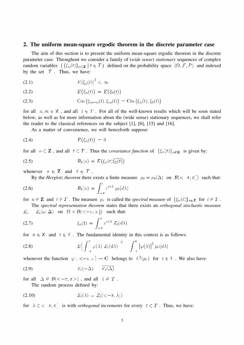
2. The uniform mean-square ergodic theorem in the discrete parameter case

The aim of this section is to present the uniform mean-square ergodic theorem in the discrete

parameter case. Throughout we consider a family of (wide sense) stationary sequences of complex

random variables�f�n(t)gn2Z j t 2 T

�defined on the probability space (;F ; P ) and indexed

by the set T . Thus, we have:

(2.1) E���n(t)��2 < 1

(2.2) E��n(t)

�= E

��0(t)

�(2.3) Cov

��m+n(t); �m(t)

�= Cov

��n(t); �0(t)

�for all n;m 2 Z , and all t 2 T . For all of the well-known results which will be soon stated

below, as well as for more information about the (wide sense) stationary sequences, we shall refer

the reader to the classical references on the subject [1], [6], [15] and [16].

As a matter of convenience, we will henceforth suppose:

(2.4) E��n(t)

�= 0

for all n 2 Z , and all t 2 T . Thus the covariance function of f�n(t)gn2Z is given by:

(2.5) Rt(n) = E��n(t)�0(t)

�whenever n 2 Z and t 2 T .

By the Herglotz theorem there exists a finite measure �t = �t(�) on B(<��; � ]) such that:

(2.6) Rt(n) =

Z �

��ein� �t(d�)

for n 2 Z and t 2 T . The measure �t is called the spectral measure of f�n(t)gn2Z for t 2 T .

The spectral representation theorem states that there exists an orthogonal stochastic measure

Zt = Zt(!;�) on � B(<��; � ]) such that:

(2.7) �n(t) =

Z �

��ein� Zt(d�)

for n 2 Z and t 2 T . The fundamental identity in this context is as follows:

(2.8) E��� Z �

��'(�) Zt(d�)

���2 =

Z �

��

��'(�)��2 �t(d�)whenever the function ' : <��; � ]! C belongs to L2(�t) for t 2 T . We also have:

(2.9) Zt(��) = Zt(�)

for all � 2 B(<��; �>) , and all t 2 T .

The random process defined by:

(2.10) Zt(�) = Zt(<��; �])for � 2<��; � ] is with orthogonal increments for every t 2 T . Thus, we have:

3

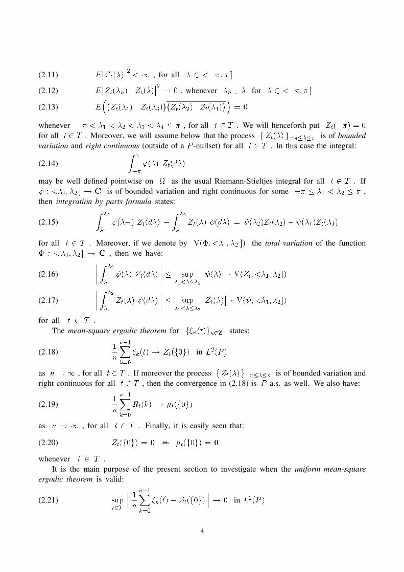
(2.11) E��Zt(�)

��2 < 1 , for all � 2 <��; � ]

(2.12) E��Zt(�n)�Zt(�)

��2 ! 0 , whenever �n # � for � 2 <��; � ](2.13) E

��Zt(�4)�Zt(�3)

��Zt(�2)�Zt(�1)

��= 0

whenever �� < �1 < �2 < �3 < �4 � � , for all t 2 T . We will henceforth put Zt(��) = 0for all t 2 T . Moreover, we will assume below that the process fZt(�)g������ is of bounded

variation and right continuous (outside of a P -nullset) for all t 2 T . In this case the integral:

(2.14)

Z �

��'(�) Zt(d�)

may be well defined pointwise on as the usual Riemann-Stieltjes integral for all t 2 T . If

: <�1; �2 ] ! C is of bounded variation and right continuous for some �� � �1 < �2 � � ,

then integration by parts formula states:

(2.15)

Z �2

�1

(��) Zt(d�) +

Z �2

�1

Zt(�) (d�) = (�2)Zt(�2)� (�1)Zt(�1)

for all t 2 T . Moreover, if we denote by V(�; <�1; �2 ]) the total variation of the function

� : <�1; �2 ] ! C , then we have:

(2.16)

���� Z �2

�1

(�) Zt(d�)

���� � sup�1<���2

�� (�)�� � V(Zt; <�1; �2 ])

(2.17)

���� Z �2

�1

Zt(�) (d�)

���� � sup�1<���2

��Zt(�)�� � V( ;<�1; �2 ])

for all t 2 T .

The mean-square ergodic theorem for f�n(t)gn2Z states:

(2.18)1

n

n�1Xk=0

�k(t) ! Zt(f0g) in L2(P )

as n!1 , for all t 2 T . If moreover the process fZt(�)g������ is of bounded variation and

right continuous for all t 2 T , then the convergence in (2.18) is P -a.s. as well. We also have:

(2.19)1

n

n�1Xk=0

Rt(k) ! �t(f0g)

as n ! 1 , for all t 2 T . Finally, it is easily seen that:

(2.20) Zt(f0g) = 0 , �t(f0g) = 0

whenever t 2 T .

It is the main purpose of the present section to investigate when the uniform mean-square

ergodic theorem is valid:

(2.21) supt2T

��� 1n

n�1Xk=0

�k(t) � Zt(f0g)��� ! 0 in L2(P )

4

as n ! 1 . We think that this problem appears worthy of consideration, and moreover to the

best of our knowledge it has not been studied previously.

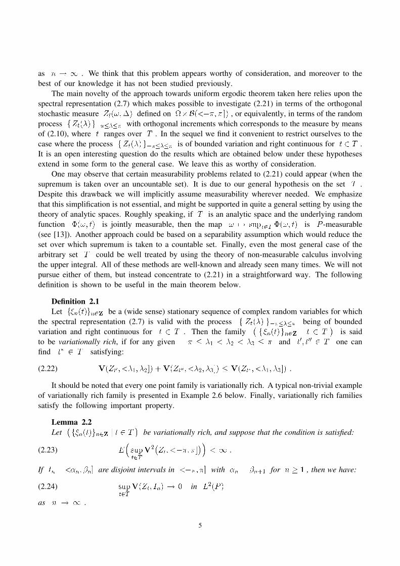
The main novelty of the approach towards uniform ergodic theorem taken here relies upon the

spectral representation (2.7) which makes possible to investigate (2.21) in terms of the orthogonal

stochastic measure Zt(!;�) defined on �B(<��; � ]) , or equivalently, in terms of the random

process fZt(�)g������ with orthogonal increments which corresponds to the measure by means

of (2.10), where t ranges over T . In the sequel we find it convenient to restrict ourselves to the

case where the process fZt(�)g������ is of bounded variation and right continuous for t 2 T .

It is an open interesting question do the results which are obtained below under these hypotheses

extend in some form to the general case. We leave this as worthy of consideration.

One may observe that certain measurability problems related to (2.21) could appear (when the

supremum is taken over an uncountable set). It is due to our general hypothesis on the set T .

Despite this drawback we will implicitly assume measurability wherever needed. We emphasize

that this simplification is not essential, and might be supported in quite a general setting by using the

theory of analytic spaces. Roughly speaking, if T is an analytic space and the underlying random

function �(!; t) is jointly measurable, then the map ! 7! supt2T �(!; t) is P -measurable

(see [13]). Another approach could be based on a separability assumption which would reduce the

set over which supremum is taken to a countable set. Finally, even the most general case of the

arbitrary set T could be well treated by using the theory of non-measurable calculus involving

the upper integral. All of these methods are well-known and already seen many times. We will not

pursue either of them, but instead concentrate to (2.21) in a straightforward way. The following

definition is shown to be useful in the main theorem below.

Definition 2.1

Let f�n(t)gn2Z be a (wide sense) stationary sequence of complex random variables for which

the spectral representation (2.7) is valid with the process f Zt(�) g������ being of bounded

variation and right continuous for t 2 T . Then the family� f�n(t)gn2Z j t 2 T

�is said

to be variationally rich, if for any given �� � �1 < �2 < �3 � � and t0; t00 2 T one can

find t� 2 T satisfying:

(2.22) V(Zt0 ; <�1; �2]) +V(Zt00; <�2; �3]) � V(Zt�; <�1; �3]) .

It should be noted that every one point family is variationally rich. A typical non-trivial example

of variationally rich family is presented in Example 2.6 below. Finally, variationally rich families

satisfy the following important property.

Lemma 2.2

Let�f�n(t)gn2Z j t 2 T

�be variationally rich, and suppose that the condition is satisfied:

(2.23) E�supt2TV2

�Zt; <��; �]

��< 1 .

If In =<�n; �n] are disjoint intervals in <��; �] with �n = �n+1 for n � 1 , then we have:

(2.24) supt2TV(Zt; In) ! 0 in L2(P )

as n ! 1 .

5

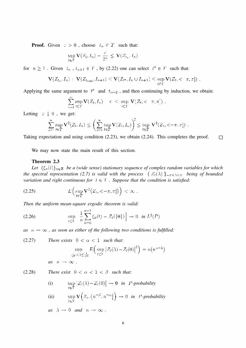
Proof. Given " > 0 , choose tn 2 T such that:

supt2TV(Zt; In) � "

2n� V(Ztn ; In)

for n � 1 . Given tn , tn+1 2 T , by (2.22) one can select t� 2 T such that:

V(Ztn; In) +V(Ztn+1 ; In+1) � V(Zt�; In [ In+1) � supt2TV(Zt; <��; �]) .

Applying the same argument to t� and tn+2 , and then continuing by induction, we obtain:1Xn=1

supt2TV(Zt; In) � " � sup

t2TV(Zt; <��; �]) .

Letting " # 0 , we get:

1Xn=1

supt2TV2(Zt; In) �

� 1Xn=1

supt2TV(Zt; In)

�2� sup

t2TV2(Zt; <��; �]) .

Taking expectation and using condition (2.23), we obtain (2.24). This completes the proof.

We may now state the main result of this section.

Theorem 2.3

Let f�n(t)gn2Z be a (wide sense) stationary sequence of complex random variables for which

the spectral representation (2.7) is valid with the process f Zt(�) g������ being of bounded

variation and right continuous for t 2 T . Suppose that the condition is satisfied:

(2.25) E�supt2TV2�Zt; <��; �]

��< 1 .

Then the uniform mean-square ergodic theorem is valid:

(2.26) supt2T

��� 1n

n�1Xk=0

�k(t) � Zt(f0g)��� ! 0 in L2(P )

as n ! 1 , as soon as either of the following two conditions is fulfilled:

(2.27) There exists 0 < � < 1 such that:

sup� 1n�

<�� 1n�

E�supt2T

��Zt(�)�Zt(0)��2� = o�n��1

�as n ! 1 .

(2.28) There exist 0 < � < 1 < � such that:

(i) supt2T

��Zt(�)�Zt(0)�� ! 0 in P -probability

(ii) supt2TV�Zt;

n��; n��

�� ! 0 in P -probability

as � ! 0 and n ! 1 .

6

Moreover, if� f�n(t)gn2Z j t 2 T

�is variationally rich, then the uniform mean-square ergodic

theorem (2.26) holds if and only if we have:

(2.29) supt2T

��Zt(�)�Zt(0) + Zt(0�)�Zt(��)�� ! 0 in P -probability

as � ! 0 . In particular, if� f�n(t)gn2Z j t 2 T

�is variationally rich, then the uniform

mean-square ergodic theorem (2.26) holds whenever the process f Zt(�) g������ is uniformly

continuous at zero:

(2.30) supt2T

��Zt(�)�Zt(0)�� ! 0 in P -probability

as � ! 0 .

Proof. Let t 2 T and n � 1 be given and fixed. Then by (2.7) we have:

1

n

n�1Xk=0

�k(t) =1

n

n�1Xk=0

Z �

��

eik� Zt(d�) =

Z �

��

'n(�) Zt(d�)

where 'n(�) = (1=n)(ein��1)=(ei��1) for � 6= 0 and 'n(0) = 1 . Hence we get:

(2.31)1

n

n�1Xk=0

�k(t) � Zt

�f0g� = Z �

��

�'n(�)�1f0g(�)

�Zt(d�) =

Z �

��

n(�) Zt(d�)

=

Z ��n

�� n(�) Zt(d�) +

Z �n

��n n(�) Zt(d�) +

Z �

�n

n(�) Zt(d�)

for any 0 < �n < � , where n(�) = '(�) for � 6= 0 and n(0) = 0 .

We begin by showing that (2.27) is sufficient for (2.26). The proof of this fact is carried out

into two steps as follows. (The first step will be of use later on as well.)

Step 1. We choose �n # 0 in (2.31) such that:

(2.32) supt2T

��� Z ��n

�� n(�) Zt(d�)

��� ! 0 in L2(P )

(2.33) supt2T

��� Z �

�n

n(�) Zt(d�)��� ! 0 in L2(P )

as n ! 1 .

First consider (2.32), and note that by (2.16) we get:

(2.34)��� Z ��n

�� n(�) Zt(d�)

��� � sup��<����n

�� n(�)�� � V�Zt; <��;��n ]

�� 2

n

1�� e�i�n�1�� � V�

Zt; <��; � ]�

.

Put �n = n�� for some � > 0 , and denote An = (1=n)(1=je�i�n�1j) . Then we have:

(2.35) A2n =

1

n21�� e�i�n�1

��2 =1

n21

2�1�cos (n��)� ! 0

as n ! 1 , if and only if � < 1 . Hence by (2.34) and (2.25) we see that (2.32) holds with

7

�n = n�� for any 0 < � < 1 .

Next consider (2.33), and note that by (2.16) we get:

(2.36)��� Z �

�n

n(�) Zt(d�)��� � 2An � V

�Zt; <��; � ]

�where An is clearly as above. Thus by the same argument we see that (2.33) holds with �n = n��for any 0 < � < 1 . (In the sequel �n is always understood in this sense.)

Step 2. Here we consider the remaining term in (2.31). First notice that from integration by

parts (2.15) we obtain the estimate:��� Z �n

��n n(�) Zt(d�)

��� � �� n(�n)�� � ��Zt(�n)�� +

�� n(��n)�� � ��Zt(��n)��+

��� Z �n

��n

�Zt(�)�Zt(0)

� n(d�)

��� +��Zt(0)�� � �� n(�n)� n(��n)�� .

Hence by Jensen’s inequality we get:

supt2T

��� Z �n

��n n(�) Zt(d�)

���2 � 4

��� n(�n)��2 � supt2T

��Zt(�n)��2 +�� n(��n)��2 � sup

t2T

��Zt(��n)��2+ V

� n; <��n; �n]

� � Z �n

��nsupt2T

��Zt(�)�Zt(0)��2 V( n; d�)+ sup

t2T

��Zt(0)��2 � �� n(�n)� n(��n)��2 � .

Taking expectation and using Fubini’s theorem we obtain:

(2.37) E

�supt2T

��� Z �n

��n n(�) Zt(d�)

���2� � 4

��� n(�n)��2 �E� supt2T

��Zt(�n)��2�+ �� n(��n)��2 �E� supt2T

��Zt(��n)��2�+ sup��n<���n

E�supt2T

��Zt(�)�Zt(0)��2� � V2� n; <��n; �n]

�+ E

�supt2T

��Zt(0)��2� � �� n(�n)� n(��n)��2 � .

Now note that for any �� < � � � we have:

jZt(�)j � jZt(�)�Zt(�t)j + jZt(�t)j � V(Zt; <��; � ]) + "

where �t is chosen to be close enough to �� to satisfy jZt(�t)j � " by right continuity.

Passing to the supremum and using (2.25) hence we get:

(2.38) E�supt2T

sup��<���

��Zt(�)��2� < 1 .

By (2.35) we have n(�n) ! 0 and n(��n) ! 0 , and thus by (2.38) we see that:

(2.39)�� n(�n)��2 � E� sup

t2T

��Zt(�n)��2� +�� n(��n)��2 � E� sup

t2T

��Zt(��n)��2�+ E

�supt2T

��Zt(0)��2� � �� n(�n)� n(��n)��2 ! 0

as n!1 . From (2.37) we see that it remains to estimate the total variation of n on <��n; �n] .

8

For this put Fk(�) = eik� for 0 � k � n � 1 , and notice that we have:

(2.40) V� n; <��n; �n ]

� � 1 + V�'n; <��n; �n ]

� � 1 +

Z �n

��nj'n0(�)j d�

By the Cauchy-Schwarz inequality and orthogonality of Fk’s on <��; �] , we obtain from (2.40)

the following estimate:

(2.41) V� n; <��n; �n ]

� � 1 +p2�n

1

n

�Z �

��

��� n�1Xk=0

ikFk(�)���2d� �1=2

=

= 1 +p2�n

1

n

� n�1Xk=1

k2�1=2

� 1 +p2�n

1

nn3=2 � Cn(1��)=2

with some constant C > 0 . Combining (2.31), (2.32), (2.33), (2.37), (2.39) and (2.41) we complete

the proof of sufficiency of (2.27) for (2.26). This fact finishes Step 2.

We proceed by showing that (2.28) is sufficient for (2.26). For this Step 1 can stayed unchanged,

and Step 2 is modified as follows.

Step 3. First split up the integral:

(2.42)Z �n

��n n(�) Zt(d�) =

Z ��n

��n n(�) Zt(d�) +

Z �n

��n n(�) Zt(d�) +

Z �n

�n

n(�) Zt(d�)

for any 0 < �n < �n . Put �n = n�� for some � > 1 . (In the sequel �n is always understood

in this sense.) Then from (2.9) and (2.16) we get by right continuity:

(2.43)��� Z ��n

��n n(�) Zt(d�)

��� � V�Zt; <��n;��n ]

�= V

�Zt; [��n;��n ]

�= V

�Zt; [�n; �n ]

�= V

�Zt; <�n; �n ]

�.

Similarly, by (2.16) we get:

(2.44)��� Z �n

�n

n(�) Zt(d�)��� � V

�Zt; <�n; �n ]

�.

From (2.25), (2.43), (2.44) and (ii) in (2.28) it follows by uniform integrability that:

(2.45) supt2T

��� Z ��n

��n n(�) Zt(d�)

��� ! 0 in L2(P )

(2.46) supt2T

��� Z �n

�n

n(�) Zt(d�)��� ! 0 in L2(P )

as n!1 . Now by (2.31), (2.32), (2.33), (2.45) and (2.46) we see that it is enough to show:

(2.47) supt2T

��� Z �n

��n n(�) Zt(d�)

��� ! 0 in L2(P )

as n!1 . For this recall n(0) = 0 . Thus from integration by parts (2.15) with (2.17) we get:

(2.48)��� Z �n

��n n(�) Zt(d�)

��� � ��� Z 0�

��n n(�) Zt(d�)

��� + ��� Z �n

0

n(�) Zt(d�)���

9

� �� n(0�)Zt(0�) � n(��n)Zt(��n)�� + ��� Z 0�

��nZt(�) n(d�)

���+�� n(�n)Zt(�n) � n(0+)Zt(0)

��+ ��� Z �n

0

Zt(�) n(d�)��� � ��Zt(0�) � n(��n)Zt(��n)

��+ sup��n<�<0

��Zt(�)�� � V� n;<��n; 0>�+ �� n(�n)Zt(�n)� Zt(0)��+ sup

0<���n

��Zt(�)�� � V� n; <0; �n]� .

Next we verify that:

(2.49) n(��n) ! 1 & n(�n) ! 1

as n ! 1 . For this note that we have:

�� n(��n)�1�� = ��� 1n

n�1Xk=0

e�ik�n�1��� � max

0�k�n�1��e�ik�n�1��

=��e�i(n�1)�n�1

�� � ��e�i(1=n��1)�1�� ! 0

as n ! 1 . This proves (2.49). In addition we show that:

(2.50) V� n;<��n; 0>

� ! 0 & V� n; <0; �n ]

� ! 0

as n ! 1 . For this note that we have:

V� n; <0; �n]

� � 1

n

n�1Xk=0

V�Fk; <0; �n]

� � max0�k�n�1

V�Fk; <0; �n ]

�= V

�Fn�1; <0; �n ]

� � ��1�cos �n�� + �� sin �n�� ! 0

as n ! 1 . In the same way we obtain:

V� n; <��n; 0>

� � ��1�cos�n�� + �� sin �n�� ! 0

as n ! 1 . Thus (2.50) is established. Finally, we obviously have:

(2.51)��Zt(0�)� n(��n)Zt(��n)

�� � ��Zt(0�)�Zt(��n)�� + ��1� n(��n)�� � ��Zt(��n)

��(2.52)

�� n(�n)Zt(�n)�Zt(0)�� � �� n(�n)�1

�� � ��Zt(�n)�� + ��Zt(�n)�Zt(0)

�� .

Combining (2.28), (2.38), (2.48), (2.49), (2.50), (2.51) and (2.52) we obtain (2.47). This fact

completes the proof of sufficiency of (2.28) for (2.26). Step 3 is complete.

A slight modification of Step 3 will show that (2.29) is sufficient for (2.26) whenever the family

is variationally rich. This is done in the next step.

Step 4. First consider the left side in (2.48). By (2.15) and (2.17) we have:��� Z �n

��n n(�) Zt(d�)

��� � ��� Z 0�

��n n(�) Zt(d�) +

Z �n

0

n(�) Zt(d�)���

� �� n(0�)Zt(0�)� n(��n)Zt(��n) + n(�n)Zt(�n)� n(0+)Zt(0)��

+��� Z 0�

��nZt(�) n(d�)

���+ ��� Z �n

0

Zt(�) n(d�)��� � �� n(�n)�1

�� � ��Zt(�n)��

10

+��Zt(�n)�Zt(0) + Zt(0�)�Zt(��n)

�� + ��1� n(��n)�� � ��Zt(��n)��+ sup��n<�<0

��Zt(�)�� � V� n; <��n; 0>

�+ sup

0<���n

��Zt(�)�� � V� n; <0; �n]

�.

Hence by the same arguments as in Step 3 we obtain (2.47).

Next consider the remaining terms in (2.42). By (2.43) and (2.44) we see that it suffices to show:

(2.53) V�Zt; <�n; �n ]

� ! 0 in L2(P )

as n ! 1 . We show that (2.53) holds with �n = n�3=2 and �n = n�1=2 . The general case

follows by the same pattern (with possibly a three intervals argument in (2.55) below).

For this put In =<�n; �n ] , and let pn = (pn�1)3 for n � 2 with p1 = 2 . Then the

intervals Ipn satisfy the hypotheses of Lemma 2.2 for n � 1 , and therefore we get:

(2.54) supt2T

V�Zt; Ipn

� ! 0 in L2(P )

as n ! 1 . Moreover, for pn < q � pn+1 we have:

(2.55) V�Zt; Iq

� � V�Zt; Ipn

�+ V

�Zt; Ipn+1

�.

Thus from (2.54) we obtain (2.53), and the proof of sufficiency of (2.29) for (2.26) follows as in

Step 3. This fact completes Step 4.

In the last step we prove necessity of (2.29) for (2.26) under the assumption that the family

is variationally rich.

Step 5. From integration by parts (2.15) we have:

1

n

n�1Xk=0

�k(t) � Zt�f0g� = Z �

�� n(�) Zt(d�) =

Z ��n

�� n(�) Zt(d�) +

Z ��n

��n n(�) Zt(d�)

+ n(0�)Zt(0�)� n(��n)Zt(��n) + n(�n)Zt(�n)� n(0+)Zt(0)

�Z 0�

��nZt(�) n(d�) �

Z �n

0

Zt(�) n(d�)

+

Z �n

�n

n(�) Zt(d�) +

Z �

�n

n(�) Zt(d�) .

Hence we easily get:

(2.56)��Zt(�n)�Zt(0) + Zt(0�)�Zt(��n)

�� � �� n(�n)�1�� � ��Zt(�n)��+ ��1� n(��n)�� � ��Zt(��n)��

+��� Z �

�� n(�) Zt(d�)

���+ ��� Z ��n

�� n(�) Zt(d�)

���+ ��� Z ��n

��n n(�) Zt(d�)

���+ ��� Z 0�

��nZt(�) n(d�)

���+��� Z �n

0

Zt(�) n(d�)��� + ��� Z �n

�n

n(�) Zt(d�)��� + ��� Z �

�n

n(�) Zt(d�)��� .

Finally, from (2.16) and (2.17) we obtain the estimates as in Step 3 and Step 4:

(2.57)��� Z 0�

��nZt(�) n(d�)

��� � sup��n<�<0

��Zt(�)�� � V� n; <��n; 0>�(2.58)

��� Z �n

0

Zt(�) n(d�)��� � sup

0<���n

��Zt(�)�� � V� n; <0; �n ]�

11

(2.59)��� Z ��n

��n n(�) Zt(d�)

��� � V�Zt; <�n; �n ]

�(2.60)

��� Z �n

�n

n(�) Zt(d�)��� � V

�Zt; <�n; �n ]

�.

Combining (2.32), (2.33), (2.38), (2.49), (2.50), (2.53), (2.56) and (2.57)-(2.60) we complete

the proof of necessity of (2.29) for (2.26). This fact finishes Step 5. The last statement of the

theorem is obvious, and the proof is complete.

Remarks 2.4

(1) Note that Theorem 2.3 reads as follows: If the convergence in (2.27) is not uniformly fast

enough (but we still have it), then examine convergence of the total variation as stated in (ii) of

(2.28). Characterization (2.29) with (2.30) shows that this approach is in some sense optimal.

(2) A close look into the proof shows that we have convergence P -a.s. in (2.26), as soon as we

have convergence P -a.s. either in (2.27) (without the expectation and square sign, but with (��1)=2),

or in (i) and (ii) of (2.28). Moreover, if�f�n(t)gn2Z j t 2 T

�is pointwise variationally rich, then

the same fact holds as for characterization (2.29), as well as for sufficient condition (2.30). In all

of these cases the condition (2.25) could be relaxed by removing the expectation and square sign.

In this way we cover a pointwise uniform ergodic theorem for (wide sense) stationary sequences.

(3) Under condition (2.25) convergence in P -probability in either (i) or (ii) of (2.28) is equivalent

to the convergence in L2(P ) . The same fact holds for convergence in P -probability in either

(2.29) or (2.30). It follows by uniform integrability.

(4) For condition (ii) of (2.28) note that for every fixed t 2 T and any 0 < � < 1 < � :

V�Zt;

n�� ; n��

�� ! 0 P -a.s.

whenever fZt(�) g������ is of bounded variation and right continuous (at zero), as n ! 1 .

Note also that under condition (2.25) the convergence is in L2(P ) as well.

(5) It is easily verified by examining the proof above that characterization (2.29) remains valid

under (2.25), whenever the property of being variationally rich is replaced with any other property

implying condition (ii) of (2.28).

(6) It remains an open interesting question does the result of Theorem 2.3 extend in some form

to the case where the associated process fZt(�)g������ is not of bounded variation for t 2 T .

Example 2.5

Consider an almost periodic sequence of random variables:

(2.61) �n(t) =Xk2Z

zk(t)ei�kn

for n 2 Z and t 2 T . In other words, for every fixed t 2 T we have:

(2.62) Random variables zi(t) and zj(t) are mutually orthogonal for all i 6= j :

E�zi(t)zj(t)

�= 0

(2.63) Numbers �k belong to <��; �] for k 2 Z , and satisfy �i 6= �j whenever i 6= j

(2.64) The condition is satisfied:

12

Xk2Z

Ejzk(t)j2 < 1 .

Note that under (2.64) the series in (2.61) converges in the mean-square sense.

From (2.61) we see that the orthogonal stochastic measure is defined as follows:

Zt(�) =X

k2Z;�k2�zk(t)

for � 2 B(<��; � ]) and t 2 T . The covariance function is given by:

Rt(n) =Xk2Z

ei�knEjzk(t)j2

for n 2 Z and t 2 T .

In order to apply Theorem 2.3 we will henceforth assume:

(2.65) E

�supt2T

�Xk2Z

jzk(t)j�2�

< 1 .

Note that this condition implies:

(2.66) E

�supt2T

�Xk2Z

jzk(t)j2��

< 1 .

Let k0 2 Z be chosen to satisfy �k0 = 0 , and otherwise conceive zk0(t) � 0 for all t 2 T .

According to Theorem 2.3, the uniform mean-square ergodic theorem is valid:

(2.67) supt2T

��� 1n

n�1Xk=0

�k(t) � zk0(t)��� ! 0 in L2(P )

as n ! 1 , as soon as either of the following two conditions is fulfilled:

(2.68) There exists 0 < � < 1 such that:

sup0<�� 1

n�

E

�supt2T

��� X0<�k��

zk(t)���2� + sup

� 1n�

<�<0

E

�supt2T

��� X�<�k�0

zk(t)���2� = o

�n��1

�as n ! 1 .

(2.69) There exist 0 < � < 1 < � such that:

(i) supt2T

��� X0<�k��

zk(t)��� + sup

t2T

��� X��<�k�0

zk(t)��� �! 0 in P -probability

(ii) supt2T

X1

n�<�j� 1

n�

jzj(t)j ! 0 in P -probability

as � # 0 and n ! 1 .

In particular, hence we see if zero does not belong to the closure of the sequence f�kgk2Z ,

then (2.67) is valid. Moreover, if the condition is fulfilled:

(2.70) E

�Xk2Z

supt2T

jzk(t)j�2

< 1

13

with zk0(t) � 0 for t 2 T , then clearly (i) and (ii) of (2.69) are satisfied, even though the condition

(2.68) on the speed of convergence could possibly fail. Thus, under (2.70) we have again (2.67).

Example 2.6 (Variationally rich family)

Consider the Gaussian case in the preceding example. Thus, suppose that the almost periodic

sequence (2.61) is given:

(2.71) �n(t) =Xk2Z

zk(t)ei�kn

for n 2 Z and t 2 T , where for every fixed t 2 T the random variables zk(t) =�k(t) � gk � N(0; �2k(t)) are independent and Gaussian with zero mean and variance �2k(t)for k 2 Z . Then (2.62) is fulfilled. We assume that (2.63) and (2.64) hold. Thus, the family

� =� f�2k(t)gk2Z j t 2 T

�satisfies the following condition:

(2.72)Xk2Z

�2k(t) < 1

for all t 2 T . We want to see when the family � =� f�n(t)gn2Z j t 2 T

�is variationally rich,

and this should be expressed in terms of the family � .

For this, take arbitrary �� � �1 < �2 < �3 � � and t0 , t00 2 T , and compute the left-hand

side in (2.22). From the form of the orthogonal stochastic measure Zt = Zt(!;�) which is

established in the preceding example, we see that:

(2.73) V (Zt;�) =X

k2Z;�k2�jzk(t)j

for � 2 B(<��; � ]) and t 2 T . Hence we find:

(2.74) V(Zt0; <�1; �2 ]) + V(Zt00; <�2; �3 ])

=X

�1<�k��2

���k(t0)��jgkj +X

�2<�k��3

���k(t00)��jgkj .

Thus, in order that � is variationally rich, the expression in (2.74) must be dominated by:

(2.75)X

�1<�k��3

���k(t�)��jgkjfor some t� 2 T . For instance, this will be true if the family � satisfies the following property:

(2.76)��2k(t

0)_�2k(t00)k2Z 2 �

for all t0 , t00 2 T . For example, if �k(t) = t=2jkj for k 2 Z and t belongs to a subset T of

< 0;1> , the last property (2.76) is satisfied, and the family � is variationally rich.

3. The uniform mean-square ergodic theorem in the continuous parameter case

The aim of this section is to present the uniform mean-square ergodic theorem in the continuous

parameter case. Throughout we consider a family of (wide sense) stationary processes of complex

random variables�fXs(t)gs2R j t 2 T

�defined on the probability space (;F ; P ) and indexed

14

by the set T . Thus, we have:

(3.1) E��Xs(t)

��2 < 1(3.2) E

�Xs(t)

�= E

�X0(t)

�(3.3) Cov

�Xr+s(t); Xr(t)

�= Cov

�Xs(t); X0(t)

�for all s; r 2 R , and all t 2 T . For the same reasons as in Section 2 we shall refer the reader

to the classical references on the subject [1], [6] and [15].

As a matter of convenience, we will henceforth suppose:

(3.4) E�Xs(t)

�= 0

for all s 2 R , and all t 2 T . Thus the covariance function of fXs(t)gs2R is given by:

(3.5) Rt(s) = E�Xs(t)X0(t)

�whenever s 2 R and t 2 T .

By the Bochner theorem there exists a finite measure �t = �t(�) on B(R) such that:

(3.6) Rt(s) =

Z 1

�1eis� �t(d�)

for s 2 R and t 2 T . The measure �t is called the spectral measure of fXs(t)gs2R for t 2 T .

The spectral representation theorem states if Rt is continuous, then there exists an orthogonal

stochastic measure Zt = Zt(!;�) on � B(R) such that:

(3.7) Xs(t) =

Z 1

�1eis� Zt(d�)

for s 2 R and t 2 T . The fundamental identity in this context is as follows:

(3.8) E��� Z 1

�1'(�) Zt(d�)

���2 = Z 1

�1

��'(�)��2 �t(d�)whenever the function ' : R ! C belongs to L2(�t) for t 2 T . We also have (2.9) which

is valid for all � 2 B(R) , and all t 2 T .

The random process defined by:

(3.9) Zt(�) = Zt(<�1; �])

for � 2 R is with orthogonal increments for every t 2 T . Thus, we have (2.11), (2.12) and

(2.13) whenever � 2 R and �1 < �1 < �2 < �3 < �4 < 1 for all t 2 T . We will

henceforth put Zt(�1) = 0 for all t 2 T . Moreover, we will assume below again that the

process f Zt(�) g�2R is of bounded variation and right continuous (outside of a P -nullset) for

all t 2 T . In this case the integral:

(3.10)

Z 1

�1'(�) Zt(d�)

may be well defined pointwise on as the usual Riemann-Stieltjes integral for all t 2 T . If

15

: <�1; �2 ]! C is of bounded variation and right continuous for some �1 � �1 < �2 � 1 ,

then integration by parts formula (2.15) holds for all t 2 T . Moreover, for the total variation

V(�; <�1; �2 ]) of the function � : <�1; �2]! C we have (2.16) and (2.17) for all t 2 T .

The mean-square ergodic theorem for fXs(t)gs2R states:

(3.11)1

�

Z �

0Xs(t) ds ! Zt(f0g) in L2(P )

as � ! 1 , for all t 2 T . If moreover the process fZt(�) g�2R is of bounded variation and

right continuous for all t 2 T , then the convergence in (3.11) is P -a.s. as well. We also have:

(3.12)1

�

Z �

0Rt(s) ds ! �t(f0g)

as � ! 1 , for all t 2 T . Finally, it is easily seen that (2.20) is valid in the present case

whenever t 2 T .

It is the main purpose of the present section to investigate when the uniform mean-square

ergodic theorem is valid:

(3.13) supt2T

��� 1�

Z �

0Xs(t) ds � Zt(f0g)

��� ! 0 in L2(P )

as � !1 . As before, we think that this problem appears worthy of consideration, and moreover

to the best of our knowledge it has not been studied previously. It turns out that the methods

developed in the last section carry over to the present case without any difficulties.

The main novelty of the approach could be explained in the same way as in Section 2. The

same remark might be also directed to the measurability problems. We will not state either of this

more precisely here, but instead recall that we implicitly assume measurability wherever needed.

The definition stated in Section 2 extends verbatim to the present case. Again, it is shown to

be useful in the main theorem below.

Definition 3.1

Let fXs(t)gs2R be a (wide sense) stationary process of complex random variables for which

the spectral representation (3.7) is valid with the process fZt(�)g�2R being of bounded variation

and right continuous for t 2 T . Then the family�fXs(t)gs2R j t 2 T

�is said to be variationally

rich, if for any given �1 < �1 < �2 < �3 <1 and t0; t00 2 T one can find t� 2 T satisfying:

(3.14) V(Zt0; <�1; �2]) +V(Zt00; <�2; �3]) � V(Zt�; <�1; �3]) .

We remark again that every one point family is variationally rich. A typical non-trivial example

of variationally rich family in the present case may be constructed similarly as in Example 2.6 above.

Finally, variationally rich families satisfy the following important property.

Lemma 3.2

Let�fXs(t)gs2R j t 2 T

�be variationally rich, and suppose that the condition is satisfied:

(3.15) E�supt2TV2

�Zt;R

��< 1 .

If In =<�n; �n] are disjoint intervals in R with �n = �n+1 for n � 1 , then we have:

16

(3.16) supt2TV(Zt; In) ! 0 in L2(P )

as n ! 1 .

Proof. The proof is exactly the same as the proof of Lemma 2.2. The only difference is that

the interval <��; � ] should be replaced with R .

We may now state the main result of this section.

Theorem 3.3

Let fXs(t)gs2R be a (wide sense) stationary process of complex random variables for which

the spectral representation (3.7) is valid with the process fZt(�)g�2R being of bounded variation

and right continuous for t 2 T . Suppose that the condition is satisfied:

(3.17) E�supt2TV2

�Zt;R

��< 1 .

Then the uniform mean-square ergodic theorem is valid:

(3.18) supt2T

��� 1�

Z �

0Xs(t) ds � Zt(f0g)

��� ! 0 in L2(P )

as � ! 1 , as soon as either of the following two conditions is fulfilled:

(3.19) There exists 0 < � < 1 such that:

sup����<�����

E�supt2T

��Zt(�)�Zt(0)��2� = o����1

�as � ! 1 .

(3.20) There exist 0 < � < 1 < � such that:

(i) supt2T

��Zt(�)�Zt(0)�� ! 0 in P -probability

(ii) supt2TV�Zt;

��� ; ���

�� ! 0 in P -probability

as � ! 0 and � ! 1 .

Moreover, if the family�fZs(t)gs2R j t 2 T

�is variationally rich, then the uniform mean-square

ergodic theorem (3.18) holds if and only if we have:

(3.21) supt2T

��Zt(�)�Zt(0) + Zt(0�)�Zt(��)�� ! 0 in P -probability

as � ! 0 . In particular, if the family� fZs(t)gs2R j t 2 T

�is variationally rich, then the

uniform mean-square ergodic theorem (3.18) holds whenever the process fZt(�)g�2R is uniformly

continuous at zero:

(3.22) supt2T

��Zt(�)�Zt(0)�� ! 0 in P -probability

as � ! 0 .

17

Proof. The proof may be carried out by using precisely the same method which is presented

in the proof of Theorem 2.3. Thus we find it unnecessary here to provide all of the details, but

instead will turn out only the essential points which make the procedure working.

Let � > 0 be fixed. We begin by noticing that a simple Riemann approximation yields:nX

k=1

�

nexp

�ik

�

n��!Z �

0

eis� ds

as n!1 , for all � 2 R . Since the left side above is bounded by constant function � which

belongs to L2(�t) , then by (3.8) we get:Z 1�1

� nXk=1

�

nexp

�ik�

n���

Zt(d�) =

nXk=1

�

nXk �n

(t) !Z 1�1

�Z �

0

eis� ds�Zt(d�) in L2(P )

as n ! 1 , for all t 2 T . Hence we get:

1

�

Z �

0

Xs(t) ds =

Z 1

�1f� (�) Zt(d�)

for all t 2 T , where f� (�) = (1=�)(ei���1)=(i�) for � 6= 0 and f� (0) = 1 . Thus we have:

1

�

Z �

0

Xs(t) ds � Zt(f0g) =Z 1

�1

�f� (�) � 1f0g(�)

�Zt(d�) =

Z 1

�1g� (�) Zt(d�)

for all t 2 T , where g� (�) = f� (�) for � 6= 0 and g� (0) = 0 .

Let us first reconsider Step 1. For this note that by (2.16) we get:

(3.23)��� Z ���

��g� (�) Zt(d�)

��� � sup�1<�����

��g� (�)�� � V�Zt; <�1;��� ]

� � 2

�

1

j i�� j � V�Zt;R

�for all t 2 T . Thus putting �� = ��� for some � > 0 , we see that:

(3.24) supt2T

��� Z ���

�1g� (�) Zt(d�)

��� ! 0 in L2(P )

as � !1 , as soon as we have 0 < � < 1 . In exactly the same way as for (3.24) we find:

(3.25) supt2T

��� Z 1

��

g� (�) Zt(d�)��� ! 0 in L2(P )

as � ! 1 . Facts (3.24) and (3.25) complete Step 1.

Next reconsider Step 2. First, it is clear that:

(3.26) g� (��� ) ! 0 & g� (�� ) ! 0

as � ! 1 . Next, by the same arguments as in the proof of Theorem 2.3 we obtain:

(3.27) E�supt2T

sup�2R

jZt(�)j2�< 1 .

Thus the only what remains is to estimate the total variation of g� on <��� ; �� ] .

For this put Gs(�) = eis� for 0 � s � � , and notice that we have:

(3.28) V�g� ; <��� ; �� ]

� � 1 + V�f� ; <��� ; �� ]

� � 1 +

Z ��

���

jf�0(�)j d� .

18

Next recall that f� (�) = (1=�)R �0 eis� ds for all � 2 R . Again, by the Cauchy-Schwarz

inequality (with Fubini’s theorem) and orthogonality of Gs’s on <��; �] , we obtain from (3.28):

(3.29) V�g� ; <��� ; �� ]

� � 1 +p2��

1

�

�Z �

��

��� Z �

0

is � Gs(�) ds���2d��1=2

=

= 1 +p2��

1

�

�Z �

0

s2 ds�1=2

= 1 +p2��

1

�

� 3=2p3� C� (1��)=2

with some constant C > 0 . Finally, by using (3.26), (3.27) and (3.29) we can complete Step 2

as in the proof of Theorem 2.3.

To complete Step 3 as in the proof of Theorem 2.3, it is just enough to verify that:

(3.30) g� (��� ) ! 1 & g� (�� ) ! 1

(3.31) V�g� ; <��� ; 0>

� ! 0 & V�g� ; <0; �� ]

� ! 0

as � ! 1 , where �� = n�� for � > 1 .

First consider (3.30), and note that we have:��g� (��� )�1�� = ��� 1�

Z �

0

e�is�� ds� 1��� � sup

0�s��

��e�is���1�� = ��e�i����1

�� = ��e�i(1=���1)�1��! 0

as � ! 1 . This proves (3.30).

Next consider (3.31), and note that we have:

V�g� ; <0; �� ]

� � 1

�

Z �

0

V�Gs; <0; �� ]

�ds � sup

0�s��V�Gs; <0; �� ]

�= V

�G� ; <0; �� ]

�� ��1�cos ��

�� + �� sin �� �� ! 0

as � !1 . This proves the second part of (3.31). The first part follows by the same argument.

The rest of the proof can be carried out as it was done in the proof of Theorem 2.3.

We conclude by pointing out that Remarks 2.4 carry over in exactly the same form to cover

the present case. The same remark might be directed to Example 2.5 and Example 2.6.

Acknowledgment. Thanks are due to S. E. Graversen for improving upon the original draft of

(2.41), and to J. Hoffmann-Jørgensen for his constant advice and support.

REFERENCES

[1] ASH, R. B. and GARDNER, M. F. (1975). Topics in Stochastic Processes. Academic Press.

[2] BLUM, J. R. (1955). On the convergence of empiric distribution functions. Ann. Math.

Statist. 26 (527-529).

[3] CANTELLI, F. P. (1933). Sulla determinazione empirica della leggi di probabilita. Giorn.

Ist. Ital. Attuari 4 (421-424).

[4] DEHARDT, J. (1971). Generalizations of the Glivenko-Cantelli theorem. Ann. Math. Statist.

42 (2050-2055).

19

[5] DUDLEY, R. M. (1984). A course on empirical processes. Ecole d’Ete de Probabilities de

Saint-Flour, XII-1982. Lecture Notes in Math. 1097, Springer-Verlag (1-142).

[6] GIHMAN, I. I. and SKOROHOD, A. V. (1974, 1975, 1979). Theory of Stochastic Processes

I, II, III. Springer-Verlag, New York-Berlin.

[7] GINE, J. and ZINN, J. (1984). Some limit theorems for empirical processes. Ann. Probab.

12 (929-989).

[8] GLIVENKO, V. I. (1933). Sulla determizaione empirica della leggi di probabilita. Giorn. Ist.

Ital. Attuari 4 (92-99).

[9] HOFFMANN-JØRGENSEN, J. (1984). Necessary and sufficient conditions for the uniform law

of large numbers. Proc. Probab. Banach Spaces V (Medford 1984), Lecture Notes in Math.

1153, Springer-Verlag Berlin Heidelberg (258-272).

[10] HOFFMANN-JØRGENSEN, J. (1990). Uniform convergence of martingales. Proc. Probab.

Banach Spaces VII (Oberwolfach 1988), Progr. Probab. Vol. 21, Birhauser, Boston, 1994,

(127-137).

[11] PESKIR, G. (1992). Uniform convergence of reversed martingales. Math. Inst. Aarhus,

Preprint Ser. No. 21, (27 pp). J. Theoret. Probab. 8, 1995 (387-415).

[12] PESKIR, G. and WEBER, M. (1992). Necessary and sufficient conditions for the uniform

law of large numbers in the stationary case. Math. Inst. Aarhus, Preprint Ser. No. 27, (26

pp). Proc. Funct. Anal. IV (Dubrovnik 1993), Various Publ. Ser. Vol. 43, 1994 (165-190).

[13] PESKIR, G. and WEBER, M. (1993). The uniform ergodic theorem for dynamical systems.

Math. Inst. Aarhus, Preprint Ser. No. 14, (30 pp). Proc. Convergence in Ergodic Theory

and Probability (Columbus 1993), Ohio State Univ. Math. Res. Inst. Publ. Vol. 5, Walter

de Gruyter, Berlin, 1996 (305-332).

[14] PESKIR, G. and YUKICH, J. E. (1993). Uniform ergodic theorems for dynamical systems

under VC entropy conditions. Math. Inst. Aarhus, Preprint Ser. No. 15, (25 pp). Proc.

Probab. Banach Spaces IX (Sandbjerg 1993), Progr. Probab. Vol. 35, Birhauser, Boston,

1994 (104-127).

[15] ROZANOV, Yu. A. (1967). Stationary Random Processes. Holden-Day.

[16] SHIRYAYEV, A. N. (1984). Probability. Springer-Verlag New York.

[17] TALAGRAND, M. (1987). The Glivenko-Cantelli problem. Ann. Probab. 15 (837-870).

[18] VAPNIK, V. N. and CHERVONENKIS, A. Ya. (1971). On the uniform convergence of relative

frequencies of events to their probabilities. Theory Probab. Appl. 16 (264-280).

[19] VAPNIK, V. N. and CHERVONENKIS, A. Ya. (1981). Necessary and sufficient conditions for

the uniform convergence of means to their expectations. Theory Probab. Appl. 26 (532-553).

[20] YUKICH, J. E. (1985). Sufficient conditions for the uniform convergence of means to their

expectations. Sankhya Ser. A 47 (203-208).

Goran Peskir, Department of Mathematical Sciences, University of Aarhus, Denmark,

Ny Munkegade, DK-8000 Aarhus, home.imf.au.dk/goran, goran@imf.au.dk

20