THE U N I F I E D THEORY OF EXPLOSIONS WITH F U E L C O N S U M P T I O N

B. F. GRAY

School o f Chemistry, Macquar ie University, Sydney N S W 2113, Austral ia

A technique already successfully applied to the problem of 'fuel consumption' in thermal explosions is here applied to the related problems arising in the isothermal chain theory of explosions and the more general unified (chain-thermal) theory of explosions. T h e new results all reduce satisfactorily to known cases. It is shown that typical isothermal problems can be dealt with analytically and an explicit expression found for the induction period. Some nonisothermal problems can also be dealt with analytically to zeroth approximations and even when this is not possible a clear qualitative picture of the physical phenomena occurring is given. Quantitative data can be obtained by computation without difficulty as the problem is clearly formulated mathematically when analytical treatment is not possible.

Introduction

The original formulations of thermal explosion theory, ~ isothermal branched chain explosion theory ~ and unified chain-thermal explosion theory ~-7 all ignored the variation in time of the concentrations of the original reactants. With this assumption all these theories give clearly defined critical conditions or bifurcations which have been identified physically with the boundary in parameter space between explosive and non-explosive behav- iour.

If the variation of original reactants is included in the formulation then the bifurcations exhibited by the equations disappear (here we are talking about closed systems). Formal definition of the explosion limit then becomes a difficult conceptual problem as no discontinuities occur.

A considerable amount of effort has gone into the examination of this problem for thermal explo- sion theory s-*7 and the problem can be regarded as solved in principle and in practice if a mild degree of computation is carried out.

Strangely, the isothermal theory has apparently not been examined as to the effects of fuel consump- tion. More understandably neither has the rather more complex unified theory. Of course results obtained for the unified theory should reduce to the special cases of the two simpler theories as they indeed do when fuel consumption is ignored. The aim of this project is to commence the study of the effect of fuel consumption on the unified theory. As a necessary preliminary the effect of fuel con-

sumption in an isothermal explosive system is con- sidered.

An Isothermal Example

Consider the kinetic scheme

k t

A---~ x k b

x + B--, 2x k t

x + A---, Inert Product

The appropriate differential equations describing this scheme are

d x i

- - = k , A ' + (kbB' - k , A ' ) x ' d t

dA' = - k , A ' - k , A ' x ' (1)

dt

dB' . . . . kb B, x,

d t

but it is much more convenient to use the dimen- sionless variables, x = x ' /x~, , A = A ' / A ' , , , B = B ' / B ' o w h e r e x ' o, A' o and B',, are the in i t ia l c o n c e n t r a t i o n s o f x, A and B. We assume that x is an uns t ab le radical or i n t e rmed ia t e so that X'o < < A'o = B'o. H e n c e we in t roduce the

927

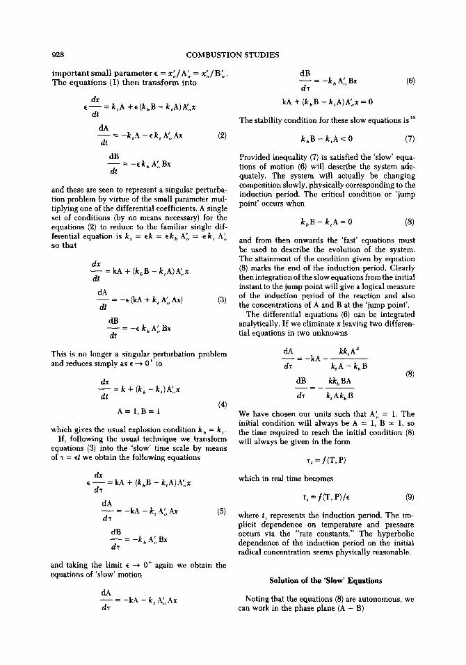
928 COMBUSTION STUDIES

impor tan t smal l pa rame te r ~ = x' , lA~, = x~,lB',,. The equa t ions (1) t h e n t ransform into

dx - - = k , A +~(khB - k,A)A',,x dt

dA = - k , A - e k, A', Ax (2)

dt

dB - - = - c k s A~, Bx dt

and these are seen to represent a singular perturba- tion problem by virtue of the small parameter mul- tiplying one of the differential coefficients. A single set of conditions (by no means necessary) for the equations (2) to reduce to the familiar single dif- ferential equation is k~ = ~k = ~k h A',, = ~k t A~, so that

dx - - = kA + (khB - k,A)A',,x dt

dA - - = - r + k , A',, Ax) (3) dt

dB - - = - c k b A~, Bx dt

This is no longer a singular perturbation problem and reduces simply as t ~ 0 + to

dx - - = k + (k b - k,)A', ,x d t

A - = I , B - ~ I (4)

which gives the usual explosion condition k s = k,. If, following the usual technique we transform

equations (3) into the 'slow' time scale by means of "r = ~t we obtain the following equations

dx

dr = kA + (kbB - k,A)A' , ,x

dA = - k A - k, A',, Ax (5)

d r

dB - - = - k b A~, Bx d r

and taking the limit t ---} 0 + again we obtain the equations of 'slow' motion

dA = - k A - k , A~, Ax

dr

dB = - k s A',, B x (6)

dx

kA + (kbB - k,A)A' , ,x = 0

The stability condition for these slow equations is is

k b B - k,A < 0 (7)

Provided inequality (7) is satisfied the 'slow' equa- tions of motion (6) will describe the system ade- quately. The system will actually be changing composition slowly, physically corresponding to the induction period. The critical condition or ' jump point' occurs when

k b B - k , A = 0 (8)

and from then onwards the 'fast' equations must be used to describe the evolution of the system. The attainment of the condition given by equation (8) marks the end of the induction period. Clearly then integration of the slow equations from the initial instant to the jump point will give a logical measure of the induction period of the reaction and also the concentrations of A and B at the 'jump point'.

The differential equations (6) can be integrated analytically. If we eliminate x leaving two differen- tial equations in two unknowns

dA kk, A ~ - - = - k A dr k t A - k b B

dB kk b BA

dx k, A k b B

(8)

We have chosen our units such that A', = 1. The initial condition will always be A = 1, B = 1, so the time required to reach the initial condition (8) will always be given in the form

r, = f ( T , P )

which in real time becomes

t, = f (T , P)/~ (9)

where t , represents the induction period. The im- plicit dependence on temperature and pressure occurs via the "rate constants." The hyperbolic dependence of the induction period on the initial radical concentration seems physically reasonable.

S o l u t i o n o f t h e " S l o w ' E q u a t i o n s

Noting that the equations (8) are autonomous, we can work in the phase plane (A - B)

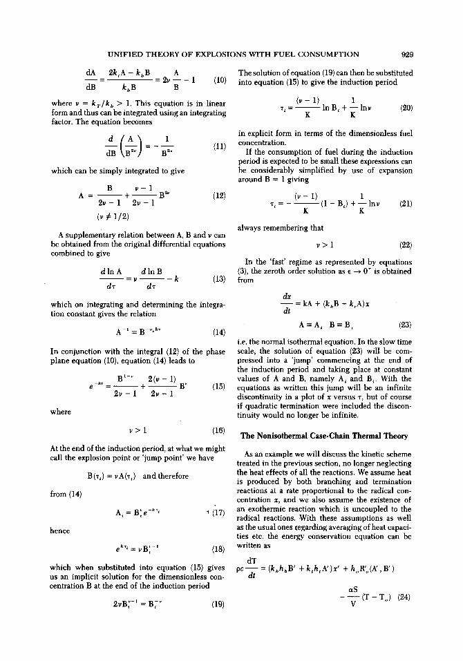
UNIFIED THEORY OF EXPLOSIONS WITH FUEL CONSUMPTION 929

dA 2k,A - khB A - - - = 2v - - - 1 (10) dB kbB B

where v = k r / k ~ > 1. This equation is in linear form and thus can be integrated using an integrating factor. The equation becomes

1

dB = B~ ~ (11)

which can be simply integrated to give

B v - 1 A - - - + B ~

2v - 1 2v - 1 (12)

(v # 1/2)

A supplementary relation between A, B and v can be obtained from the original differential equations combined to give

d l n A d l n B = v - - - k (13)

d'r d'r

which on integrating and determining the integra- tion constant gives the relation

A -1 = B - o ' k " (14)

In conjunction with the integral (12) of the phase plane equation (10), equation (14) leads to

B 1-~ 2 ( v - 1) --/or e - + B v (15) 2v - 1 2 v - 1

where

v > 1 (16)

At the end of the induction period, at what we might call the explosion point or ' jump point' we have

from (14)

hence

B(%) = vA(%) and therefore

At u -kx. = B,e ' ~ (17)

e k" = v B [ - ' (18)

which when substituted into equation (15) gives us an implicit solution for the dimensionless con- centration B at the end of the induction period

2vB~-* = B~ -~ (19)

The solution of equation (19) can then be substituted into equation (15) to give the induction period

(v - 1) 1 % - In B , + - - l n v (20)

K K

in explicit form in terms of the dimensionless fuel concentration.

If the consumption of fuel during the induction period is expected to be small these expressions can be considerably simplified by use of expansion around B = 1 giving

(v - 1) 1 x, = - - - (1 - B,) + - - lnv (21)

K K

always remembering that

v > 1 (22)

In the 'fast' regime as represented by equations (3), the zeroth order solution as e ~ 0 § is obtained from

dx = kA + (ksB - k,A)x

dt

A - A , B ~ B , (23)

i.e. the normal isothermal equation. In the slow time scale, the solution of equation (23) will be com- pressed into a 'jump' commencing at the end of the induction period and taking place at constant values of A and B, namely A, and B,. With the equations as written this jump will be an infinite discontinuity in a plot of x versus v, but of course if quadratic termination were included the discon- tinuity would no longer be infinite.

The N o n i s o t h e r m a l C a s e - C h a i n T h e r m a l Theory

As an example we will discuss the kinetic scheme treated in the previous section, no longer neglecting the heat effects of all the reactions. We assume heat is produced by both branching and termination reactions at a rate proportional to the radical con- centration x, and we also assume the existence of an exothermic reaction which is uncoupled to the radical reactions. ,With these assumptions as well as the usual ones i;egarding averaging of heat capaci- ties etc. the energy conservation equation can be written as

dT ' ' + ' ' , B ' p c - - ~ = (kbhbB' + k , h , A )x h,,R,,(b: )

aS - - - ( T - T o ) (24)

V

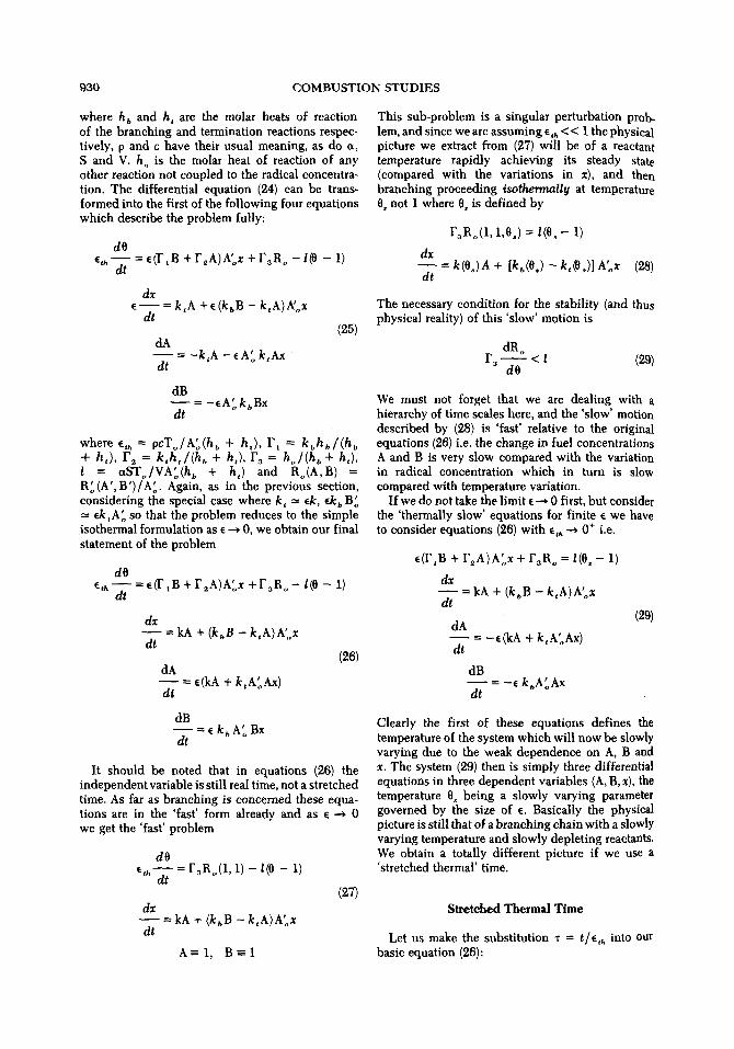
930 COMBUSTION STUDIES

where h a and h, are the molar heats of reaction of the branching and termination reactions respec- tively, p and c have their usual meaning, as do a, S and V. h o is the molar heat of reaction of any other reaction not coupled to the radical concentra- tion. The differential equation (24) can be trans- formed into the first of the following four equations which describe the problem fully:

dO e,h--7-_ = e(F~B + F~A)A'ox + FaRo - l(O - I)

dt

dx

dt = k,A +~(kbB - k ,A)A 'ox

dA = -k ,A - e A'o k , A x

d t

(25)

dB = -eA'o kaBx

d t

where e,a = pcTo /A 'o (h a + h , ) , r , = k b h b / ( h a + h , ) , r 2 = k , h , / ( h a + h,), r 3 = h o / ( h a + h,), I = a S T o / V A ' o ( h a + h,) and Bo(A,B) = R'o (A', B') /A 'o . again, as in the previous section, considering the special case where k, ~- ek, ek a B ' o = ek,A'o so that the problem reduces to the simple isothermal formulation as e --, 0, we obtain our final statement of the problem

dO e,a .--7- = e ( r , B + r~A)A'ox +F~Ro - t(0 - 1)

a t

dx = kA + (kaB - k ,A)A 'oX

dt

dA = e(kA + k,A'oAx)

d t

(26)

This sub-problem is a singular perturbation prob- lem, and since we are assuming eta < < 1 the physical picture we extract from (27) will be of a reactant temperature rapidly achieving its steady state (compared with the variations in x), and then branching proceeding i so thermal ly at temperature 0, not 1 where 0s is defined by

LBo(1, 1,0.) = ~(o.- 1) dx

= k(O.)A + [ks({}.) - k,~},)] A'ox d t

(22)

The necessary condition for the stability (and thus physical reality) of this 'slow' motion is

dRo r 3 < l (29)

dO

We must not forget that we are dealing with a hierarchy of time scales here, and the 'slow' motion described by (28) is 'fast' relative to the original equations (26) i.e. the change in fuel concentrations A and B is very slow compared with the variation in radical concentration which in turn is slow compared with temperature variation.

If we do not take the limit e ~ 0 first, but consider the 'thermally slow' equations for finite �9 we have to consider equations (26) with eth "~ 0+ i.e.

~(r,B + r~a)A'ox + r3Ro = t(O. - 1)

dx = kA + (kbB - ktA)A'x

dt

dA = -e (kA + k,A'oAx)

d t

dB . . . . e k aA'o Ax

dt

(29)

dB - - = ~ k a A ' o B X dt

It should be noted that in equations (26) the independent variable is still real time, not a stretched time. As far as branching is concerned these equa- tions are in the 'fast' form already and as e ~ 0 we get the 'fast' problem

d 8 ~ , ~ = raBo(1, 1) - ZlO - 1)

d t

dx = kA + ( kaB - k ,A)A 'o x

d t

(27)

A ~ I , B ~ I

Clearly the first of these equations defines the temperature of the system which will now be slowly varying due to the weak dependence on A, B and x, The system (29) then is simply three differential equations in three dependent variables (A, B, x), the temperature 0, being a slowly varying parameter governed by the size of e. Basically the physical picture is still that of a branching chain with a slowly varying temperature and slowly depleting reactants. We obtain a totally different picture if we use a 'stretched thermal' time.

Stretched Thermal T i m e

Let us make the substitution "r = t /~ ,h into our basic equation (26):

U N I F I E D THEORY OF EXPLOSIONS WITH FUEL CONSUMPTION 931

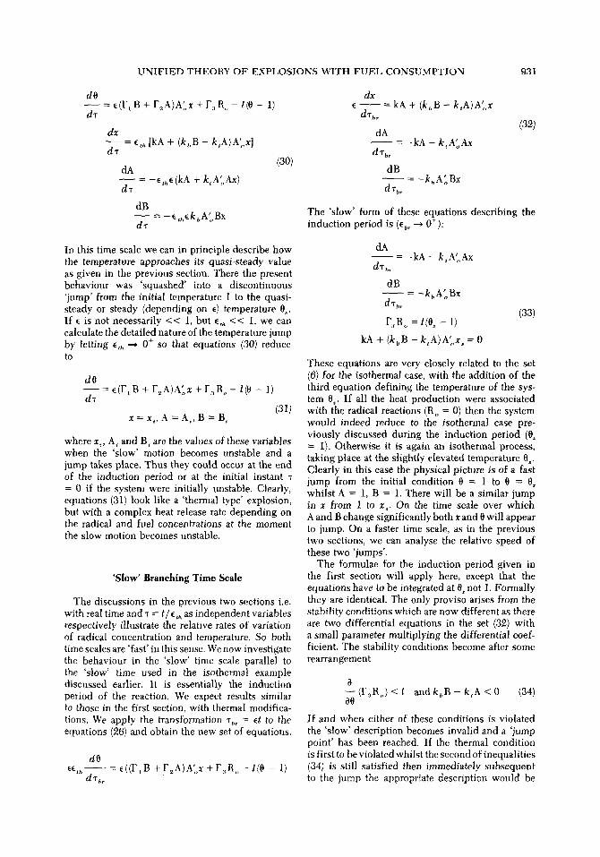
dO - - = e(F,B + F2A)A'ox + F3R ~ - l(O - 1) d-r

dx - - = %h [kA + (k~B - k,A) A'~,xl d r

dA - - = -e,he(kA + k,A'oAx) dr

dB - - = -%h~kbA~Bx d~

(30)

In this time scale we can in principle describe how the temperature approaches its quasi-steady value as given in the previous section~ There the present behaviour was 'squashed' into a discontinuous ' jump' from the initial temperature I to the quasi- steady or steady (depending on ~) temperature 02. If ~ is not necessarily < < 1, but %h < < I, we can calculate the detailed nature of the temperature jump by letting Gh "" 0+ SO that equations (30) reduce to

dO - - = ~(F~B + F2A)A'ox + F a R o - l(0 - 1) d r

(31) x = x,, A = A, ,B = B,

where x,, A, and B, are the values of these variables when the 'slow' motion becomes unstable and a jump takes place. Thus they could occur at the end of the induction period or at the initial instant r = 0 if the system were initially unstable. Clearly, equations (31) look like a 'thermal type' explosion, but with a complex heat release rate depending on the radical and fuel concentrations at the moment the slow motion becomes unstable.

' S l o w ' B r a n c h i n g T i m e S c a l e

The discussions in the previous two sections i.e. with real time and T = t /e~. as independent variables respect ive ly illustrate the relative rates of variation of radical concentration and temperature. So both time scales are 'fast' in this sense. We now investigate the behaviour in the 'slow' time scale parallel to the 'slow' time used in the isothermal example discussed earlier. It is essentially the induction period of the reaction. We expect results similar to those in the first section, with thermal modifica- tions. We apply the transformation %r = et to the equations (26) and obtain the new set of equations.

d O

d "r br - - = e((F,B + F2A)A~,x + F~R,, - I(0 - 1) E~ th

dx - - = kA + (kbB - k tA)A 'ox dThr

dA = - k A - k ,A 'oAx

d %,

dB - k~A'oBx

d "fbr

(321

The 'slow' form of these equations describing the induction period is (%, --~ 0+):

dA - kA - k,A'oAx

d'~ br

dB - kbA'Bx

d'rb,

F~R o = l(O~ - 1)

kA + (kbB - k,A)A'ox ̀ = 0

(33)

These equations are very closely related to the set (6) for the isothermal case, with the addition of the third equation defining the temperature of the sys- tem 0~. If all the heat production were associated with the radical reactions (Ro = 0) then the system would indeed reduce to the isothermal case pre- viously discussed during the induction period (0s = 1). Otherwise it is again an isothermal process, taking place at the slightly elevated temperature 0~. Clearly in this case the physical picture is of a fast jump from the initial condition 0 = 1 to 0 = 0s whilst A = 1, B = 1. There will be a similar jump in x from 1 to x,. On the time scale over which A and B change significantly both x and 0 will appear to jump, On a faster time scale, as in the previous two sections, we can analyse the relative speed of these two 'jumps'.

The formulae for the induction period given in the first section will apply here, except that the equations have to be integrated at 0 not 1. Formally they are identical. The only proviso arises from the stability conditions which are now different as there are two differential equations in the set (32) with a small parameter multiplying the differential coef- ficient. The stability conditions become after some rearrangement

- - ( F a R o ) < / a n d k b B - ktA < 0 (34) O0

If and when either of these conditions is violated the 'slow' description becomes invalid and a 'jump point ' has been reached. If the thermal condition is first to be violated whilst the second of inequalities (34) is still satisfied then immediately s u b s e q u e n t to the jump the appropriate description would be

932 COMBUSTION STUDIES

via equations (31) in what we have called stretched thermal time. The temperature varies rapidly but x remains steady. If R, were such that thermal multistability were possible it is conceivable that the end of the ' jump' could be a second stable steady state which would then ultimately become unstable a second time due to branching. More complex phenomena of this sort will be discussed elsewhere.

If, on the other hand, the second of conditions (34) is first to be violated, then the appropriate description of the 'jump' would be by use of equa- tions (27) and the reduced form (28) where the radical concentration varies rapidly compared with the tem- perature (both of course varying rapidly compared with A and B).

Conclusions

1. There are no difficulties in principle or in practice in the incorporation of 'fuel consumption' into isothermal theories of explosion. Explicit ana- lytical solutions for the induction period and the variation of reactants during this period can some- times be obtained. A description in terms of 'slow' and 'fast' regimes gives a solution including fuel decay which is continuous but with a discontinuous derivative with respect to time, the discontinuity having a clear physical interpretation.

2. There are no difficulties, in principle, in incor- porating fuel consumption into the unified (chain- thermal) theory of explosion. However the tempera- ture variation precludes analytical solution as a function of time in this case. Nevertheless the description in terms of 'slow' and 'fast' times again gives a clear physical picture of the behavior of the system.

3. In the unified theory there may be more than one small parameter present in the equations. This gives rise to a hierarchy of limiting motions e.g. temperature variation > > radical variation > > fuel variation or radical variation > > temperature varia- tion > > fuel variation.

The simplest approximation is to work in a time scale appropriate to the fuel variation in which case both temperature and radical concentrations under- go 'jumps'. Further analysis of these jumps shows that there are two limiting forms corresponding to purely thermal or purely isothermal discontinuities.

The theory thus reduces to all known cases satisfac- torily.

4. Inclusion of 'fuel consumption' into a unified model uncovers the possibility of qualitatively new phenomena such as limited nonperiodic jumps of temperature with little change in radical concentra- tion or limited nonperiodic radical jumps with little change in radical concentration. These require fur- ther investigation, but it seems possible that they are already known experimentally in multistage ignitions.

REFERENCES

1. SEMEr~OV, N.N.: Z. Phys. 48, 571 (1928). 2, SEMENOV, N.N.: Some Problems in Chemical

Kinetics and Reactivity, vol. 2, Pergamon, Lon- don (1958).

3. GRAY, B. F. AND YaNG, C. N.: J. Phys. Chem. 69, 2747 (1965).

4. YANG, C. H.: J. Phys. Chem. 73, 3407 (1969). 5. GRAY, B. F. AND YANG, C. H.: J. Phys. Chem.

73, 3395 (1969). 6. GRAY, B. F.: Trans. Farad. Soc. 65, 1603 (1969)

and 66, 1118 (1970). 7. GRAY, B. F. AND YA~G, C. H.: Trans. Farad. Soc.

65, 2133 (1969). 8. FRANr:-KAmEr~ETSKn, D. A.: Diffusion and Heat

Exchange in Chemical Kinetics, Princeton U.P. (1955).

9. THOMAS, P. N.: Proc. Roy. Soc. A262, 192 (1961). 10. ADLER, J. AND ENIG, J.: Combustion and Flame

8, 97 (1964). 11. TODES, O. M.: Acta Phys. U.R.S.S. 5, 785 (1936). 12. GRAY, B. F. AND SHEaRINGTON, M. E.: Combustion

and Flame 19, 435 and 445 (1972). 13. GRAY, B. F.: Combustion and Flame 21, 313

and 317 (1973). 14. BowEs, B. G. ANO THOMAS, P. H.: Brit. J. App.

Phys., 12, 222 (1961). 15. RICE, O. K., ALLEn, A. D. AND CAMPBELL, N. C.:

J. Am. Chem. Soc. 57, 2212 (1935). 16. GRAY, P. AND SHERRIN(ZTON, M. E.: Gas Kinetics

and Energy Transfer, vol. 2, Chemical Society, London (1976).

17. GRAY, B. F.: Combustion and Flame 24, 43 (1975).

18. ANDr~ONOV, A. A., VITT~ A. A. AND KRAUlIN, S. E.: Theory of Oscillators, Pergamon (1966).

COMMENTS

G. C. Wake, Victoria University, New Zealand. The singular perturbation method you have used in the isothermal case (scaling the time, etc.) could

be used in the more general model without the simplifying assumption you have made. Also you could presumably calculate the next couple of terms

U N I F I E D THEORY O F E X P L O S I O N S W I T H F U E L C O N S U M P T I O N 933

in the express ions for the concentrat ions as a series in e.

Authors" Reply. The next terms in the expansion in ~ could be calculated, but my feeling is that they are not warranted within the general ph i losophy of this type of work where, one is quite happy with solut ions wi th 'corners ' on.

T. Boddington, University of Leeds, England. You have not ment ioned a third case of great interest which occurs when the two small parameters have the same order of magnitude. Would you please say someth ing about this case? Does your approach allow the evaluation of the time taken to approach the quasis teady evolut ion curves from possibly re- mote initial condi t ions? What is known about the range of attraction of the quasisteady curves?

Authors" Reply. In the case when the two small

parameters are the same order of magnitude, it is not possible to separate the temporal behaviour of the radicals from that of the temperature and one f inishes up wi th a chain thermal explosion which is not well approximated either by thermal or iso- thermal models. This case shou ld not be confused wi th the case where neither of the parameters is small, so that the depletion of the original reactants cannot be separated from the radical and temperature variation. In this case, fortunately there are no st i ffness problems in a purely numerical approach.

In the approximations used here, the motion towards the quasisteady curves is, in the zeroth approximat ion a d iscont inuous jump, and in the first approximat ion it can be evaluated by integration of the 'fast ' equat ions starting from the initial condi- tions. The range of attraction of the quasis teady curves can usual ly be seen clearly (if the dimen- sionali ty of the problem is not too high) by examina- tion of the curve of s low motion in the region where it is unstable. It acts as a clearly defined watershed dividing the regions of attraction of the various b ranches of the quasisteady curves.