The Uncertainty Principle in the Presence of Quantum Memory∗

Mario Berta,1, 2 Matthias Christandl,1, 2 Roger Colbeck,3, 1, 4 Joseph M. Renes,5 and Renato Renner1

1Institute for Theoretical Physics, ETH Zurich, 8093 Zurich, Switzerland.2Faculty of Physics, Ludwig-Maximilians-Universitat Munchen, 80333 Munich, Germany.

3Perimeter Institute for Theoretical Physics, 31 Caroline Street North, Waterloo, ON N2L 2Y5, Canada.4Institute of Theoretical Computer Science, ETH Zurich, 8092 Zurich, Switzerland.

5Institute for Applied Physics, Technische Universitat Darmstadt, 64289 Darmstadt, Germany.(Dated: 1st March 2011)

The uncertainty principle, originally formu-lated by Heisenberg [1], dramatically illustratesthe difference between classical and quantum me-chanics. The principle bounds the uncertaintiesabout the outcomes of two incompatible measure-ments, such as position and momentum, on aparticle. It implies that one cannot predict theoutcomes for both possible choices of measure-ment to arbitrary precision, even if informationabout the preparation of the particle is availablein a classical memory. However, if the particleis prepared entangled with a quantum memory,a device which is likely to soon be available [2],it is possible to predict the outcomes for bothmeasurement choices precisely. In this work westrengthen the uncertainty principle to incorpo-rate this case, providing a lower bound on theuncertainties which depends on the amount of en-tanglement between the particle and the quantummemory. We detail the application of our resultto witnessing entanglement and to quantum keydistribution.

Uncertainty relations constrain the potential knowl-edge one can have about the physical properties of a sys-tem. Although classical theory does not limit the knowl-edge we can simultaneously have about arbitrary prop-erties of a particle, such a limit does exist in quantumtheory. Even with a complete description of its state, itis impossible to predict the outcomes of all possible mea-surements on the particle. This lack of knowledge, oruncertainty, was quantified by Heisenberg [1] using thestandard deviation (which we denote by ∆R for an ob-servable R). If the measurement on a given particle ischosen from a set of two possible observables, R and S,the resulting bound on the uncertainty can be expressedin terms of the commutator [3]:

∆R ·∆S ≥ 1

2|〈[R,S]〉|.

In an information-theoretic context, it is more natural toquantify uncertainty in terms of entropy rather than the

∗The published version of this work can be found in NaturePhysics 6, 659–662 (2010) at http://www.nature.com/nphys/

journal/vaop/ncurrent/abs/nphys1734.html.

standard deviation. Bia lynicki-Birula and Mycielski [4]derived entropic uncertainty relations for position andmomentum and Deutsch [5] later proved a relation thatholds for any pair of observables. Subsequently, Kraus [6]conjectured an improvement of Deutsch’s result whichwas later proven by Maassen and Uffink [7]. The im-proved relation is

H(R) +H(S) ≥ log2

1

c, (1)

where H(R) denotes the Shannon entropy of the prob-ability distribution of the outcomes when R is mea-sured. The term 1

c quantifies the complementarity ofthe observables. For non-degenerate observables, c :=maxj,k |〈ψj |φk〉|2 where |ψj〉 and |φk〉 are the eigenvec-tors of R and S, respectively.

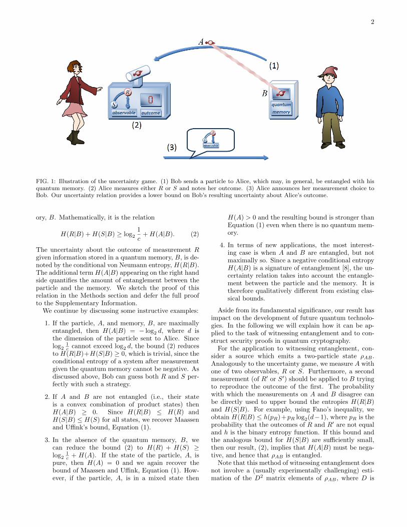
One way to think about uncertainty relations is viathe following game (the uncertainty game) between twoplayers, Alice and Bob. Before the game commences, Al-ice and Bob agree on two measurements, R and S. Thegame proceeds as follows: Bob prepares a particle in aquantum state of his choosing and sends it to Alice. Al-ice then performs one of the two measurements and an-nounces her choice to Bob. Bob’s task is to minimize hisuncertainty about Alice’s measurement outcome. This isillustrated in Figure 1.

Equation (1) bounds Bob’s uncertainty in the case thathe has no quantum memory—all information Bob holdsabout the particle is classical, e.g., a description of itsdensity matrix. However, with access to a quantum mem-ory, Bob can beat this bound. To do so, he should maxi-mally entangle his quantum memory with the particle hesends to Alice. Then, for any measurement she chooses,there is a measurement on Bob’s memory which gives thesame outcome as Alice obtains. Hence, the uncertaintiesabout both observables, R and S, vanish, which showsthat if one tries to generalize Equation (1) by replacingthe measure of uncertainty about R and S used there(the Shannon entropy) by the entropy conditioned on theinformation in Bob’s quantum memory, the resulting re-lation no longer holds.

We proceed by stating our uncertainty relation, whichapplies in the presence of a quantum memory. It providesa bound on the uncertainties of the measurement out-comes which depends on the amount of entanglement be-tween the measured particle, A, and the quantum mem-

arX

iv:0

909.

0950

v4 [

quan

t-ph

] 1

Mar

201

1

2

FIG. 1: Illustration of the uncertainty game. (1) Bob sends a particle to Alice, which may, in general, be entangled with hisquantum memory. (2) Alice measures either R or S and notes her outcome. (3) Alice announces her measurement choice toBob. Our uncertainty relation provides a lower bound on Bob’s resulting uncertainty about Alice’s outcome.

ory, B. Mathematically, it is the relation

H(R|B) +H(S|B) ≥ log2

1

c+H(A|B). (2)

The uncertainty about the outcome of measurement Rgiven information stored in a quantum memory, B, is de-noted by the conditional von Neumann entropy, H(R|B).The additional term H(A|B) appearing on the right handside quantifies the amount of entanglement between theparticle and the memory. We sketch the proof of thisrelation in the Methods section and defer the full proofto the Supplementary Information.

We continue by discussing some instructive examples:

1. If the particle, A, and memory, B, are maximallyentangled, then H(A|B) = − log2 d, where d isthe dimension of the particle sent to Alice. Sincelog2

1c cannot exceed log2 d, the bound (2) reduces

to H(R|B)+H(S|B) ≥ 0, which is trivial, since theconditional entropy of a system after measurementgiven the quantum memory cannot be negative. Asdiscussed above, Bob can guess both R and S per-fectly with such a strategy.

2. If A and B are not entangled (i.e., their stateis a convex combination of product states) thenH(A|B) ≥ 0. Since H(R|B) ≤ H(R) andH(S|B) ≤ H(S) for all states, we recover Maassenand Uffink’s bound, Equation (1).

3. In the absence of the quantum memory, B, wecan reduce the bound (2) to H(R) + H(S) ≥log2

1c + H(A). If the state of the particle, A, is

pure, then H(A) = 0 and we again recover thebound of Maassen and Uffink, Equation (1). How-ever, if the particle, A, is in a mixed state then

H(A) > 0 and the resulting bound is stronger thanEquation (1) even when there is no quantum mem-ory.

4. In terms of new applications, the most interest-ing case is when A and B are entangled, but notmaximally so. Since a negative conditional entropyH(A|B) is a signature of entanglement [8], the un-certainty relation takes into account the entangle-ment between the particle and the memory. It istherefore qualitatively different from existing clas-sical bounds.

Aside from its fundamental significance, our result hasimpact on the development of future quantum technolo-gies. In the following we will explain how it can be ap-plied to the task of witnessing entanglement and to con-struct security proofs in quantum cryptography.

For the application to witnessing entanglement, con-sider a source which emits a two-particle state ρAB .Analogously to the uncertainty game, we measure A withone of two observables, R or S. Furthermore, a secondmeasurement (of R′ or S′) should be applied to B tryingto reproduce the outcome of the first. The probabilitywith which the measurements on A and B disagree canbe directly used to upper bound the entropies H(R|B)and H(S|B). For example, using Fano’s inequality, weobtain H(R|B) ≤ h(pR)+pR log2(d−1), where pR is theprobability that the outcomes of R and R′ are not equaland h is the binary entropy function. If this bound andthe analogous bound for H(S|B) are sufficiently small,then our result, (2), implies that H(A|B) must be nega-tive, and hence that ρAB is entangled.

Note that this method of witnessing entanglement doesnot involve a (usually experimentally challenging) esti-mation of the D2 matrix elements of ρAB , where D is

3

the dimension of AB—it is sufficient to estimate the twoprobabilities pR and pS , which can be obtained by sep-arate measurements on each of the two particles. Ourmethod also differs significantly from the standard ap-proach which is based on collecting measurement statis-tics to infer the expectation values of fixed witness ob-servables on the joint system of both particles [9–12]. Weremark that when using our procedure, the best choice ofAlice’s observables are ones with high complementarity,1c .

As a second application, we consider quantum key dis-tribution. In the 1970s and 80s, Wiesner [13], and Ben-nett and Brassard [14] proposed new cryptographic pro-tocols based on quantum theory, most famously the BB84quantum key distribution protocol [14]. Their intuitionfor security lay in the uncertainty principle. In spite ofproviding the initial intuition, the majority of securityproofs to date have not involved uncertainty relations(see e.g. [15–20]), although [21] provides a notable excep-tion. The obstacle for the use of the uncertainty principleis quickly identified: a full proof of security must takeinto account a technologically unbounded eavesdropper,i.e. one who potentially has access to a quantum mem-ory. In the following, we explain how to use our mainresult, (2), to overcome this obstacle and derive a simplebound on the key rate.

Based on an idea by Ekert [22], the security of quantumkey distribution protocols is usually analysed by assum-ing that the eavesdropper creates a quantum state, ρABE ,and distributes the A and B parts to the two users, Al-ice and Bob. In practice, Alice and Bob do not providethe eavesdropper with this luxury, but a security proofthat applies even in this case will certainly imply securitywhen Alice and Bob distribute the states themselves. Inorder to generate their key, Alice and Bob measure thestates they receive using measurements chosen at ran-dom, with Alice’s possible measurements denoted by Rand S and Bob’s by R′ and S′. To ensure that the samekey is generated, they communicate their measurementchoices to one another. In the worst case, this commu-nication is overheard in its entirety by the eavesdropperwho is trying to obtain the key. Even so, Alice and Bobcan generate a secure key if their measurement outcomesare sufficiently well correlated.

To show this, we use a result of Devetak and Win-ter [8] who proved that the amount of key Alice andBob are able to extract per state, K, is lower boundedby H(R|E) − H(R|B). In addition, we reformulate ourmain result, (2), as H(R|E) + H(S|B) ≥ log2

1c , a form

previously conjectured by Boileau and Renes [23] (seethe Supplementary Information). Together these implyK ≥ log2

1c −H(R|B)−H(S|B). Furthermore, using the

fact that measurements cannot decrease entropy, we have

K ≥ log2

1

c−H(R|R′)−H(S|S′).

This corresponds to a generalization of Shor andPreskill’s famous result [17], which is recovered in the

case of conjugate observables applied to qubits and as-suming symmetry, i.e. H(R|R′) = H(S|S′). The argu-ment given here applies only to collective attacks but canbe extended to arbitrary attacks using the post-selectiontechnique [24].

This security argument has the advantage that Aliceand Bob only need to upper bound the entropies H(R|R′)and H(S|S′). Similarly to the case of entanglement wit-nessing, these entropies can be directly bounded by ob-servable quantities, such as the frequency with which Al-ice and Bob’s outcomes agree. No further informationabout the state is required. This improves the perfor-mance of practical quantum key distribution schemes,where the amount of statistics needed to estimate statesis critical for security [25].

The range of application of our result, (2), is not re-stricted to these two examples, but extends to other cryp-tographic scenarios [26], a quantum phenomenon knownas locking of information [27] (in the way presentedin [28]), and to decoupling theorems which are frequentlyused in coding arguments [23].

Finally, we note that uncertainty may be quantifiedin terms of alternative entropy measures. In fact, ourproof involves smooth entropies, which can be seen asgeneralizations of the von Neumann entropy [20] (see theMethods and Supplementary Information). These gen-eralizations have direct operational interpretations [29]and are related to physical quantities, such as thermo-dynamic entropy. We therefore expect a formulation ofthe uncertainty relation in terms of these generalized en-tropies to have further use both in quantum informationtheory and beyond.

Methods

Here we outline the proof of the main result, (2). Thequantities appearing there are evaluated for a state ρAB ,where we use H(R|B) to denote the conditional von Neu-mann entropy of the state∑

j

(|ψj〉〈ψj | ⊗ 11)ρAB(|ψj〉〈ψj | ⊗ 11),

and likewise for H(S|B).The proof is fully based on the smooth entropy calcu-

lus introduced in [20] and proceeds in three steps (werefer the reader to the Supplementary Information forfurther details, including precise definitions of the quan-tities used in this section). In the first step, which weexplain in more detail below, an uncertainty relation isproven which is similar to (2) but with the von Neumannentropy being replaced by the min- and max-entropies,denoted Hmin and Hmax (we also use H−∞ which playsa role similar to Hmax):

Hmin(R|B) +H−∞(SB) ≥ log2

1

c+Hmin(AB) . (3)

4

The quantities H−∞ and Hmin only involve the extremaleigenvalues of an operator, which makes them easier todeal with than the von Neumann entropy which dependson all eigenvalues. In the second, technically most in-volved step of the proof, we extend the relation to thesmooth min- and max-entropies, which are more generaland allow us to recover the relation for the von Neumannentropy as a special case.

The ε-smooth min- and max-entropies are formed bytaking the original entropies and extremizing them overa set of states ε-close to the original (where closenessis quantified in terms of the maximum purified distancefrom the original). In this step we also convert H−∞ toa smooth max-entropy and obtain the relation

H5√ε

min (R|B) +Hεmax(SB) ≥

log2

1

c+Hε

min(AB)− 2 log2

1

ε, (4)

which holds for any ε > 0.To complete the proof, we evaluate the inequality on

the n-fold tensor product of the state in question, i.e.on ρ⊗n. We then use the asymptotic equipartition the-orem [20, 30], which tells us that the smooth min- andmax-entropies tend to the von Neumann entropy in theappropriate limit, i.e.

limε→0

limn→∞

1

nHε

min /max(An|Bn)ρ⊗n = H(A|B)ρ.

Hence, on both sides of (4), we divide by n and take thelimit as in the previous equation to obtain

H(R|B) +H(SB) ≥ log2

1

c+H(AB),

from which our main result, (2), follows by subtractingH(B) from both sides.

We now sketch the first step of the proof. This developsan idea from [23, 28] where uncertainty relations whichonly apply to the case of complementary observables (i.e.those related by a Fourier transform) are derived. Theserelations were originally expressed in terms of von Neu-mann entropies rather than min- and max-entropies.

We use two chain rules and strong subadditivity ofthe min-entropy, to show that, for a system composed of

subsystems A′B′AB and for a state Ω,

Hmin(A′B′AB)Ω −H−∞(A′AB)Ω (5)

chain 1≤ Hmin(B′|A′AB)Ω|Ω

str.sub.≤ Hmin(B′|AB)Ω|Ω

chain 2≤ Hmin(B′A|B)Ω −Hmin(A|B)Ω. (6)

We now apply this relation to the state ΩA′B′AB de-fined as follows:

ΩA′B′AB :=1

d2

∑a,b

|a〉〈a|A′ ⊗ |b〉〈b|B′ ⊗

(DaRD

bS ⊗ 11)ρAB(D−bS D−aR ⊗ 11) ,

where |a〉a and |b〉b are orthonormal bases on d-dimensional Hilbert spaces HA′ and HB′ respectively,and DR and DS are the operators that dephase in therespective eigenbases of R and S. Hence, tracing outA′ (B′) reduces the state to one where the system, A,is measured in the eigenbasis of R (S) and the outcomeforgotten. We then use properties of the entropies to re-late the second term in (5) and the first term in (6) toH−∞(SB) and Hmin(R|B), respectively, in spite of thefact that R and S neither commute nor anticommute—aproperty that makes it difficult to complete the proof di-rectly with the von Neumann entropy. The first termof (5) is easily related to Hmin(AB). Finally, tracing outboth A′ and B′ reduces the state to one where the sys-tem, A, is measured first with one observable and thenwith the other and the outcomes forgotten. Hence, thelast term in (6) can be related to the overlap of the eigen-vectors of the two observables, c.

Bringing everything together, we obtain the desireduncertainty relation (3).

Acknowledgements: We thank Robert Konig,Jonathan Oppenheim and Marco Tomamichel for usefuldiscussions and Lıdia del Rio for the illustration (Fig-ure 1). MB and MC acknowledge support from the Ger-man Science Foundation (DFG) and the Swiss NationalScience Foundation. JMR acknowledges the support ofCASED (www.cased.de). RC and RR acknowledge sup-port from the Swiss National Science Foundation.

[1] Heisenberg, W. Uber den anschaulichen Inhalt der quan-tentheoretischen Kinematik und Mechanik. Zeitschriftfur Physik 43, 172–198 (1927).

[2] Julsgaard, B., Sherson, J., Cirac, J. I., Fiurasek, J. &Polzik, E. S. Experimental demonstration of quantummemory for light. Nature 432, 482–486 (2004).

[3] Robertson, H. P. The uncertainty principle. PhysicalReview 34, 163–164 (1929).

[4] Bia lynicki-Birula, I. & Mycielski, J. Uncertainty relationsfor information entropy in wave mechanics. Communica-

tions in Mathematical Physics 44, 129–132 (1975).[5] Deutsch, D. Uncertainty in quantum measurements.

Physical Review Letters 50, 631–633 (1983).[6] Kraus, K. Complementary observables and uncertainty

relations. Physical Review D 35, 3070–3075 (1987).[7] Maassen, H. & Uffink, J. B. Generalized entropic uncer-

tainty relations. Physical Review Letters 60, 1103–1106(1988).

[8] Devetak, I. & Winter, A. Distillation of secret key andentanglement from quantum states. Proceedings of the

5

Royal Society A: Mathematical, Physical and EngineeringSciences 461, 207–235 (2005).

[9] Horodecki, M., Horodecki, P. & Horodecki, R. Separabil-ity of mixed states: necessary and sufficient conditions.Physics Letters A 223, 1–8 (1996).

[10] Terhal, B. M. Bell inequalities and the separability cri-terion. Physics Letters A 271, 319–326 (2000).

[11] Lewenstein, M., Kraus, B., Cirac, J. I. & Horodecki, P.Optimization of entanglement witnesses. Physical ReviewA 62, 1–16 (2000).

[12] Guhne, O. & Toth, G. Entanglement detection. PhysicsReports 747, 1–75 (2009).

[13] Wiesner, S. Conjugate coding. Sigact News 15, 78–88(1983). Originally written c. 1970 but unpublished.

[14] Bennett, C. H. & Brassard, G. Quantum cryptography:Public key distribution and coin tossing. In Proceedingsof IEEE International Conference on Computers, Sys-tems and Signal Processing, Bangalore, India, 175–179(IEEE, 1984).

[15] Deutsch, D. et al. Quantum privacy amplification and thesecurity of quantum cryptography over noisy channels.Physical Review Letters 77, 2818–2821 (1996).

[16] Lo, H.-K. & Chau, H. F. Unconditional security of quan-tum key distribution over arbitrarily long distances. Sci-ence 283, 2050–2056 (1999).

[17] Shor, P. W. & Preskill, J. Simple proof of security ofthe BB84 quantum key distribution protocol. PhysicalReview Letters 85, 441–444 (2000).

[18] Christandl, M., Renner, R. & Ekert, A. A generic se-curity proof for quantum key distribution (2004). URLhttp://arxiv.org/abs/quant-ph/0402131.

[19] Renner, R. & Konig, R. Universally composable privacyamplification against quantum adversaries. In Theory ofCryptography Conference, TCC 2005, vol. 3378 of LectureNotes in Computer Science, 407–425 (Springer, 2005).

[20] Renner, R. Security of Quantum Key Distribution. Ph.D.

thesis, ETH Zurich (2005). URL http://arxiv.org/

abs/quant-ph/0512258.[21] Koashi, M. Unconditional security of quantum key distri-

bution and the uncertainty principle. Journal of Physics:Conference Series 36, 98–102 (2006).

[22] Ekert, A. Quantum cryptography based on Bell’s theo-rem. Physical Review Letters 67, 661–663 (1991).

[23] Renes, J. M. & Boileau, J.-C. Conjectured strong com-plementary information tradeoff. Physical Review Letters103, 020402 (2009).

[24] Christandl, M., Konig, R. & Renner, R. PostselectionTechnique for Quantum Channels with Applications toQuantum Cryptography. Physical Review Letters 102,020504 (2009).

[25] Renner, R., & Scarani, V. Quantum Cryptographywith Finite Resources: Unconditional Security Bound forDiscrete-Variable Protocols with One-Way Postprocess-ing. Physical Review Letters 100, 200501 (2008).

[26] Chandran, N., Fehr, S., Gelles, R., Goyal, V. & Ostro-vsky, R. Position-Based Quantum Cryptography. (2010).URL http://arxiv.org/abs/1005.1750.

[27] DiVincenzo, D. P., Horodecki, M., Leung, D. W., Smolin,J. A. & Terhal, B. M. Locking classical correlationsin quantum states. Physical Review Letters 92, 067902(2004).

[28] Christandl, M. & Winter, A. Uncertainty, monogamyand locking of quantum correlations. IEEE Transactionson Information Theory 51, 3159–3165 (2005).

[29] Konig, R., Renner, R. & Schaffner, C. The OperationalMeaning of Min- and Max-Entropy. IEEE Transactionson Information Theory 55, 4337–4347 (2009).

[30] Tomamichel, M., Colbeck, R. & Renner, R. A fully quan-tum asymptotic equipartition property. IEEE Transac-tions on information theory 55, 5840–5847 (2009).

6

Supplementary Information

Here we present the full proof of our main result, the uncertainty relation given in Equation (2) of the mainmanuscript (Theorem 1 below).

In order to state our result precisely, we introduce a few definitions. Consider two measurements described byorthonormal bases |ψj〉 and |φk〉 on a d-dimensional Hilbert space HA (note that they are not necessarily com-plementary). The measurement processes are then described by the completely positive maps

R : ρ 7→∑j

〈ψj |ρ|ψj〉|ψj〉〈ψj | and

S : ρ 7→∑k

〈φk|ρ|φk〉|φk〉〈φk|

respectively. We denote the square of the overlap of these measurements by c, i.e.

c := maxj,k|〈ψj |φk〉|2. (1)

Furthermore, we assume that HB is an arbitrary finite-dimensional Hilbert space. The von Neumann entropy ofA given B is denoted H(A|B) and is defined via H(A|B) := H(AB) − H(B), where for a state ρ on HA we haveH(A) := −tr(ρ log ρ).

The statement we prove is then

Theorem 1. For any density operator ρAB on HA ⊗HB,

H(R|B) +H(S|B) ≥ log2

1

c+H(A|B), (2)

where H(R|B), H(S|B), and H(A|B) denote the conditional von Neumann entropies of the states (R ⊗ I)(ρAB),(S ⊗ I)(ρAB), and ρAB, respectively.

In the next section, we introduce the smooth min- and max- entropies and give some properties that will be neededin the proof.

Before that, we show that the statement of our main theorem is equivalent to a relation conjectured by Boileauand Renes [1].

Corollary 2. For any density operator ρABE on HA ⊗HB ⊗HE,

H(R|E) +H(S|B) ≥ log2

1

c. (3)

Proof. To show that our result implies (3), we first rewrite (2) as H(RB) +H(SB) ≥ log21c +H(AB) +H(B). In the

case that ρABE is pure, we have H(RB) = H(RE) and H(AB) = H(E). This yields the expression H(RE)+H(SB) ≥log2

1c + H(E) + H(B), which is equivalent to (3). The result for arbitrary states ρABE follows by the concavity of

the conditional entropy (see e.g. [2]).

That (3) implies (2) can be seen by taking ρABE as the state which purifies ρAB in (3) and reversing the argumentabove.

1. (Smooth) min- and max-entropies—definitions

As described above, we prove a generalized version of (2), which is formulated in terms of smooth min- and max-entropies. This section contains the basic definitions, while Section 5 b summarizes the properties of smooth entropiesneeded for this work. For a more detailed discussion of the smooth entropy calculus, we refer to [3–6].

We use U=(H) := ρ : ρ ≥ 0, trρ = 1 to denote the set of normalized states on a finite-dimensional Hilbert spaceH and U≤(H) := ρ : ρ ≥ 0, trρ ≤ 1 to denote the set of subnormalized states on H. The definitions below apply tosubnormalized states.

7

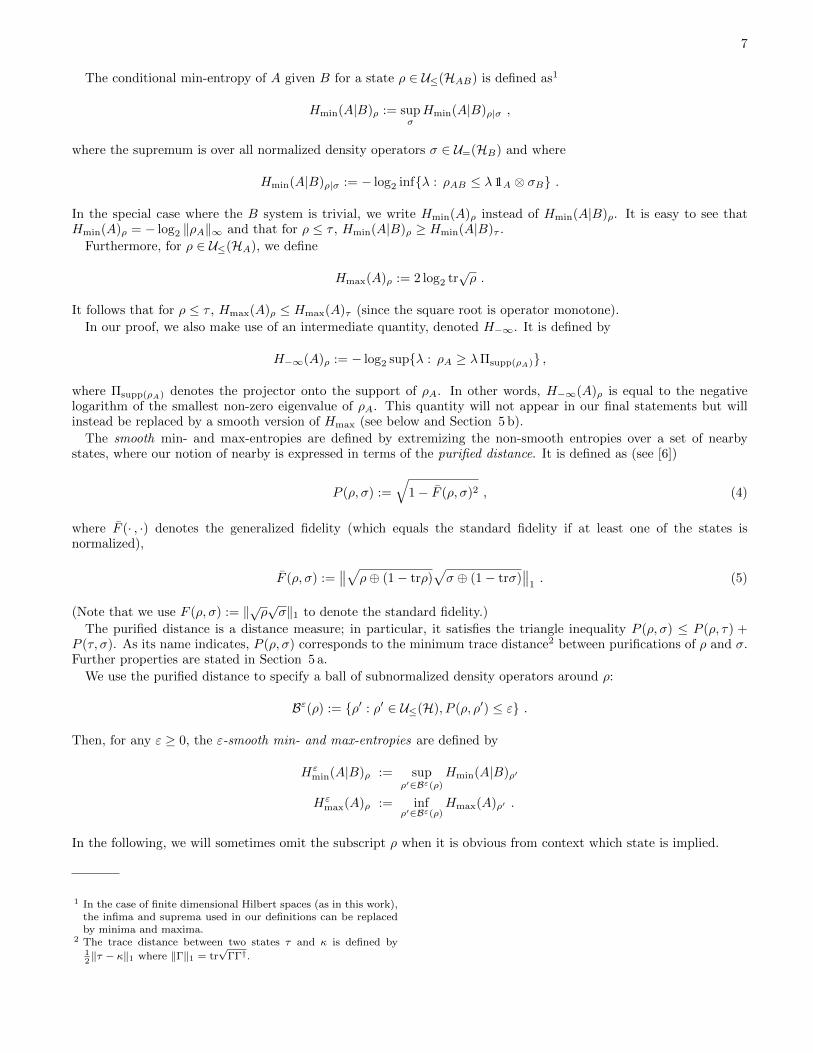
The conditional min-entropy of A given B for a state ρ ∈ U≤(HAB) is defined as1

Hmin(A|B)ρ := supσHmin(A|B)ρ|σ ,

where the supremum is over all normalized density operators σ ∈ U=(HB) and where

Hmin(A|B)ρ|σ := − log2 infλ : ρAB ≤ λ 11A ⊗ σB .

In the special case where the B system is trivial, we write Hmin(A)ρ instead of Hmin(A|B)ρ. It is easy to see thatHmin(A)ρ = − log2 ‖ρA‖∞ and that for ρ ≤ τ , Hmin(A|B)ρ ≥ Hmin(A|B)τ .

Furthermore, for ρ ∈ U≤(HA), we define

Hmax(A)ρ := 2 log2 tr√ρ .

It follows that for ρ ≤ τ , Hmax(A)ρ ≤ Hmax(A)τ (since the square root is operator monotone).

In our proof, we also make use of an intermediate quantity, denoted H−∞. It is defined by

H−∞(A)ρ := − log2 supλ : ρA ≥ λΠsupp(ρA) ,

where Πsupp(ρA) denotes the projector onto the support of ρA. In other words, H−∞(A)ρ is equal to the negativelogarithm of the smallest non-zero eigenvalue of ρA. This quantity will not appear in our final statements but willinstead be replaced by a smooth version of Hmax (see below and Section 5 b).

The smooth min- and max-entropies are defined by extremizing the non-smooth entropies over a set of nearbystates, where our notion of nearby is expressed in terms of the purified distance. It is defined as (see [6])

P (ρ, σ) :=√

1− F (ρ, σ)2 , (4)

where F (· , ·) denotes the generalized fidelity (which equals the standard fidelity if at least one of the states isnormalized),

F (ρ, σ) :=∥∥√ρ⊕ (1− trρ)

√σ ⊕ (1− trσ)

∥∥1. (5)

(Note that we use F (ρ, σ) := ‖√ρ√σ‖1 to denote the standard fidelity.)

The purified distance is a distance measure; in particular, it satisfies the triangle inequality P (ρ, σ) ≤ P (ρ, τ) +P (τ, σ). As its name indicates, P (ρ, σ) corresponds to the minimum trace distance2 between purifications of ρ and σ.Further properties are stated in Section 5 a.

We use the purified distance to specify a ball of subnormalized density operators around ρ:

Bε(ρ) := ρ′ : ρ′ ∈ U≤(H), P (ρ, ρ′) ≤ ε .

Then, for any ε ≥ 0, the ε-smooth min- and max-entropies are defined by

Hεmin(A|B)ρ := sup

ρ′∈Bε(ρ)Hmin(A|B)ρ′

Hεmax(A)ρ := inf

ρ′∈Bε(ρ)Hmax(A)ρ′ .

In the following, we will sometimes omit the subscript ρ when it is obvious from context which state is implied.

1 In the case of finite dimensional Hilbert spaces (as in this work),the infima and suprema used in our definitions can be replacedby minima and maxima.

2 The trace distance between two states τ and κ is defined by12‖τ − κ‖1 where ‖Γ‖1 = tr

√ΓΓ†.

8

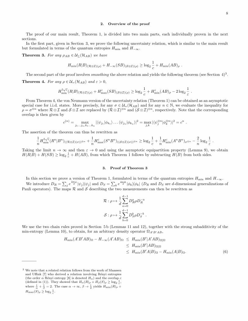
2. Overview of the proof

The proof of our main result, Theorem 1, is divided into two main parts, each individually proven in the nextsections.

In the first part, given in Section 3, we prove the following uncertainty relation, which is similar to the main resultbut formulated in terms of the quantum entropies Hmin and H−∞.

Theorem 3. For any ρAB ∈ U≤(HAB) we have

Hmin(R|B)(R⊗I)(ρ) +H−∞(SB)(S⊗I)(ρ) ≥ log2

1

c+Hmin(AB)ρ .

The second part of the proof involves smoothing the above relation and yields the following theorem (see Section 4)3.

Theorem 4. For any ρ ∈ U=(HAB) and ε > 0,

H5√ε

min (R|B)(R⊗I)(ρ) +Hεmax(SB)(S⊗I)(ρ) ≥ log2

1

c+Hε

min(AB)ρ − 2 log2

1

ε.

From Theorem 4, the von Neumann version of the uncertainty relation (Theorem 1) can be obtained as an asymptoticspecial case for i.i.d. states. More precisely, for any σ ∈ U=(HAB) and for any n ∈ N, we evaluate the inequality forρ = σ⊗n where R⊗I and S ⊗I are replaced by (R⊗I)⊗n and (S ⊗I)⊗n, respectively. Note that the correspondingoverlap is then given by

c(n) = maxj1...jn,k1...kn

|〈ψj1 |φk1〉 . . . 〈ψjn |φkn〉|2 = max

j,k|〈ψ⊗nj |φ

⊗nk 〉|

2 = cn .

The assertion of the theorem can thus be rewritten as

1

nH

5√ε

min (Rn|Bn)((R⊗I)(σ))⊗n +1

nHε

max(SnBn)((S⊗I)(σ))⊗n ≥ log2

1

c+

1

nHε

min(AnBn)σ⊗n −2

nlog2

1

ε.

Taking the limit n → ∞ and then ε → 0 and using the asymptotic equipartition property (Lemma 9), we obtainH(R|B) +H(SB) ≥ log2

1c +H(AB), from which Theorem 1 follows by subtracting H(B) from both sides.

3. Proof of Theorem 3

In this section we prove a version of Theorem 1, formulated in terms of the quantum entropies Hmin and H−∞.

We introduce DR =∑j e

2πijd |ψj〉〈ψj | and DS =

∑k e

2πikd |φk〉〈φk| (DR and DS are d-dimensional generalizations of

Pauli operators). The maps R and S describing the two measurements can then be rewritten as

R : ρ 7→ 1

d

d−1∑a=0

DaRρD

−aR

S : ρ 7→ 1

d

d−1∑b=0

DbSρD

−bS .

We use the two chain rules proved in Section 5 b (Lemmas 11 and 12), together with the strong subadditivity of themin-entropy (Lemma 10), to obtain, for an arbitrary density operator ΩA′B′AB ,

Hmin(A′B′AB)Ω −H−∞(A′AB)Ω ≤ Hmin(B′|A′AB)Ω|Ω

≤ Hmin(B′|AB)Ω|Ω

≤ Hmin(B′A|B)Ω −Hmin(A|B)Ω. (6)

3 We note that a related relation follows from the work of Maassenand Uffink [7] who derived a relation involving Renyi entropies(the order α Renyi entropy [8] is denoted Hα) and the overlap c(defined in (1)). They showed that Hα(R)ρ +Hβ(S)ρ ≥ log2

1c,

where 1α

+ 1β

= 2. The case α→∞, β → 12

yields Hmin(R)ρ +

Hmax(S)ρ ≥ log21c.

9

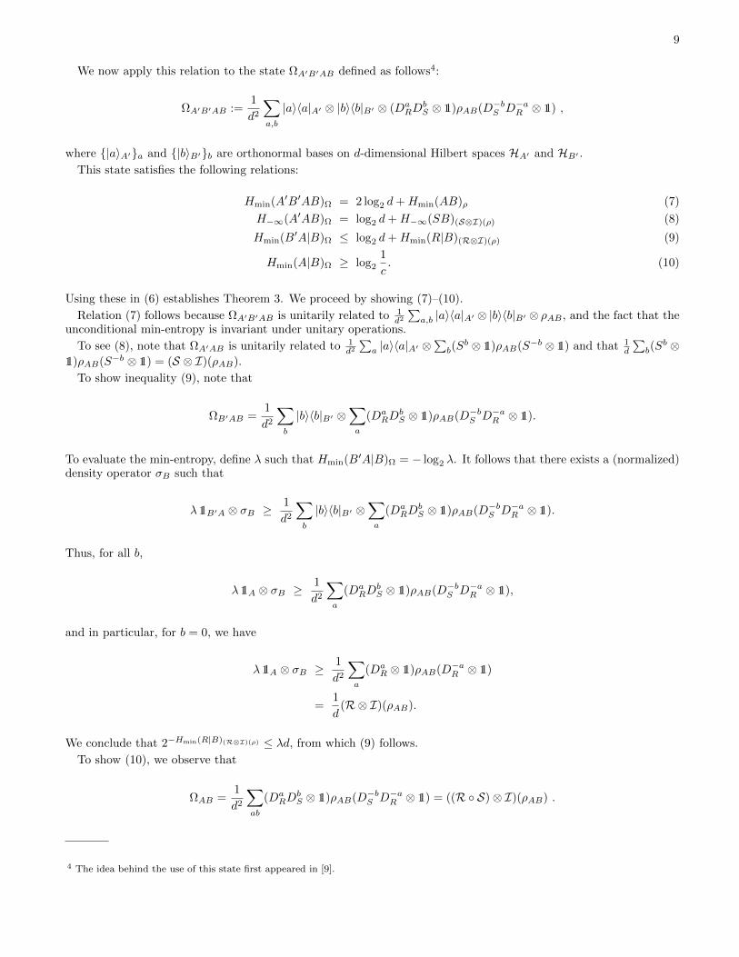
We now apply this relation to the state ΩA′B′AB defined as follows4:

ΩA′B′AB :=1

d2

∑a,b

|a〉〈a|A′ ⊗ |b〉〈b|B′ ⊗ (DaRD

bS ⊗ 11)ρAB(D−bS D−aR ⊗ 11) ,

where |a〉A′a and |b〉B′b are orthonormal bases on d-dimensional Hilbert spaces HA′ and HB′ .This state satisfies the following relations:

Hmin(A′B′AB)Ω = 2 log2 d+Hmin(AB)ρ (7)

H−∞(A′AB)Ω = log2 d+H−∞(SB)(S⊗I)(ρ) (8)

Hmin(B′A|B)Ω ≤ log2 d+Hmin(R|B)(R⊗I)(ρ) (9)

Hmin(A|B)Ω ≥ log2

1

c. (10)

Using these in (6) establishes Theorem 3. We proceed by showing (7)–(10).

Relation (7) follows because ΩA′B′AB is unitarily related to 1d2

∑a,b |a〉〈a|A′ ⊗ |b〉〈b|B′ ⊗ ρAB , and the fact that the

unconditional min-entropy is invariant under unitary operations.

To see (8), note that ΩA′AB is unitarily related to 1d2

∑a |a〉〈a|A′ ⊗

∑b(S

b ⊗ 11)ρAB(S−b ⊗ 11) and that 1d

∑b(S

b ⊗11)ρAB(S−b ⊗ 11) = (S ⊗ I)(ρAB).

To show inequality (9), note that

ΩB′AB =1

d2

∑b

|b〉〈b|B′ ⊗∑a

(DaRD

bS ⊗ 11)ρAB(D−bS D−aR ⊗ 11).

To evaluate the min-entropy, define λ such that Hmin(B′A|B)Ω = − log2 λ. It follows that there exists a (normalized)density operator σB such that

λ 11B′A ⊗ σB ≥1

d2

∑b

|b〉〈b|B′ ⊗∑a

(DaRD

bS ⊗ 11)ρAB(D−bS D−aR ⊗ 11).

Thus, for all b,

λ 11A ⊗ σB ≥1

d2

∑a

(DaRD

bS ⊗ 11)ρAB(D−bS D−aR ⊗ 11),

and in particular, for b = 0, we have

λ 11A ⊗ σB ≥1

d2

∑a

(DaR ⊗ 11)ρAB(D−aR ⊗ 11)

=1

d(R⊗ I)(ρAB).

We conclude that 2−Hmin(R|B)(R⊗I)(ρ) ≤ λd, from which (9) follows.

To show (10), we observe that

ΩAB =1

d2

∑ab

(DaRD

bS ⊗ 11)ρAB(D−bS D−aR ⊗ 11) = ((R S)⊗ I)(ρAB) .

4 The idea behind the use of this state first appeared in [9].

10

Then,

((R S)⊗ I)(ρAB) = (R⊗ I)

(∑k

|φk〉〈φk| ⊗ trA((|φk〉〈φk| ⊗ 11)ρAB)

)=∑jk

|〈φk|ψj〉|2 |ψj〉〈ψj | ⊗ trA((|φk〉〈φk| ⊗ 11)ρAB)

≤ maxlm

(|〈φl|ψm〉|2

) ∑jk

|ψj〉〈ψj | ⊗ trA((|φk〉〈φk| ⊗ 11)ρAB)

= maxlm

(|〈φl|ψm〉|2

)11A ⊗

∑k

trA((|φk〉〈φk| ⊗ 11)ρAB)

= maxlm

(|〈φl|ψm〉|2

)11A ⊗ ρB .

It follows that 2−Hmin(A|B)((RS)⊗I)(ρ) ≤ maxlm |〈φl|ψm〉|2 = c, which concludes the proof.

4. Proof of Theorem 4

The uncertainty relation proved in the previous section (Theorem 3) is formulated in terms of the entropies Hmin

and H−∞. In this section, we transform these quantities into the smooth entropies Hεmin and Hε

max, respectively, forsome ε > 0. This will complete the proof of Theorem 4.

Let σAB ∈ U≤(HAB). Lemma 15 applied to σSB := (S ⊗ I)(σAB) implies that there exists a nonnegative operatorΠ ≤ 11 such that tr((11−Π2)σSB) ≤ 3ε and

Hεmax(SB)(S⊗I)(σ) ≥ H−∞(SB)Π(S⊗I)(σ)Π − 2 log2

1

ε. (11)

We can assume without loss of generality that Π commutes with the action of S ⊗ I because it can be chosen to bediagonal in any eigenbasis of σSB . Hence, Π(S ⊗ I)(σAB)Π = (S ⊗ I)(ΠσABΠ), and

tr((11−Π2)σAB) = tr((S ⊗ I)((11−Π2)σAB)) = tr((11−Π2)σSB) ≤ 3ε . (12)

Applying Theorem 3 to the operator ΠσABΠ yields

Hmin(R|B)(R⊗I)(ΠσΠ) +HR(SB)(S⊗I)(ΠσΠ) ≥ log2

1

c+Hmin(AB)ΠσΠ . (13)

Note that ΠσΠ ≤ σ and so

Hmin(AB)ΠσΠ ≥ Hmin(AB)σ. (14)

Using (11) and (14) to bound the terms in (13), we find

Hmin(R|B)(R⊗I)(ΠσΠ) +Hεmax(SB)(S⊗I)(σ) ≥ log2

1

c+Hmin(AB)σ − 2 log2

1

ε. (15)

Now we apply Lemma 18 to ρAB . Hence there exists a nonnegative operator Π ≤ 11 which is diagonal in an eigenbasisof ρAB such that

tr((11− Π2)ρAB) ≤ 2ε (16)

and Hmin(AB)ΠρΠ ≥ Hεmin(AB)ρ. Evaluating (15) for σAB := ΠρABΠ thus gives

Hmin(R|B)(R⊗I)(ΠΠρΠΠ) +Hεmax(SB)(S⊗I)(ΠρΠ) ≥ log2

1

c+Hε

min(AB)ρ − 2 log2

1

ε, (17)

where Π is diagonal in any eigenbasis of (S ⊗ I)(ΠρABΠ) and satisfies

tr((11−Π2)ΠρABΠ) ≤ 3ε . (18)

11

Since ρAB ≥ ΠρABΠ, we can apply Lemma 17 to (S ⊗ I)(ρAB) and (S ⊗ I)(ΠρABΠ), which gives

Hεmax(SB)(S⊗I)(ρ) ≥ Hε

max(SB)(S⊗I)(ΠρΠ) . (19)

The relation (17) then reduces to

Hmin(R|B)(R⊗I)(ΠΠρΠΠ) +Hεmax(SB)(S⊗I)(ρ) ≥ log2

1

c+Hε

min(AB)ρ − 2 log2

1

ε. (20)

Finally, we apply Lemma 7 to (16) and (18), which gives

P (ρAB , ΠρABΠ) ≤√

4ε

P (ΠρABΠ,ΠΠρABΠΠ) ≤√

6ε .

Hence, by the triangle inequality

P (ρAB ,ΠΠρABΠΠ) ≤ (√

4 +√

6)√ε < 5

√ε .

Consequently, (R⊗ I)(ΠΠρABΠΠ) has at most distance 5√ε from (R⊗ I)(ρAB). This implies

H5√ε

min (R|B)(R⊗I)(ρ) ≥ Hmin(R|B)(R⊗I)(ΠΠρΠΠ) .

Inserting this in (20) gives

H5√ε

min (R|B)(R⊗I)(ρ) +Hεmax(SB)(S⊗I)(ρ) ≥ log2

1

c+Hε

min(AB)ρ − 2 log2

1

ε,

which completes the proof of Theorem 4.

5. Technical properties

a. Properties of the purified distance

The purified distance between ρ and σ corresponds to the minimum trace distance between purifications of ρ andσ, respectively [6]. Because the trace distance can only decrease under the action of a partial trace (see, e.g., [2]), weobtain the following bound.

Lemma 5. For any ρ ∈ U≤(H) and σ ∈ U≤(H),

‖ρ− σ‖1 ≤ 2P (ρ, σ).

The following lemma states that the purified distance is non-increasing under certain mappings.

Lemma 6. For any ρ ∈ U≤(H) and σ ∈ U≤(H), and for any nonnegative operator Π ≤ 11,

P (ΠρΠ,ΠσΠ) ≤ P (ρ, σ). (21)

Proof. We use the fact that the purified distance is non-increasing under any trace-preserving completely positive map(TPCPM) [6] and consider the TPCPM

E : ρ 7→ ΠρΠ⊕ tr(√

11−Π2ρ√

11−Π2).

We have P (ρ, σ) ≥ P (E(ρ), E(σ)), which implies F (ρ, σ) ≤ F (E(ρ), E(σ)). Then,

F (ρ, σ) ≤ F (E(ρ), E(σ))

= F (ΠρΠ,ΠσΠ) +√

(trρ− tr(Π2ρ))(trσ − tr(Π2σ)) +√

(1− trρ)(1− trσ)

≤ F (ΠρΠ,ΠσΠ) +√

(1− tr(Π2ρ))(1− tr(Π2σ))

= F (ΠρΠ,ΠσΠ),

which is equivalent to the statement of the Lemma.

12

The second inequality is the relation√(trρ− tr(Π2ρ))(trσ − tr(Π2σ)) +

√(1− trρ)(1− trσ) ≤

√(1− tr(Π2ρ))(1− tr(Π2σ)),

which we proceed to show. For brevity, we write trρ− tr(Π2ρ) = r, trσ − tr(Π2σ) = s, 1− trρ = t and 1− trσ = u.We hence seek to show

√rs+

√tu ≤

√(r + t)(s+ u).

For r, s, t and u nonnegative, we have√rs+

√tu ≤

√(r + t)(s+ u) ⇔ rs+ 2

√rstu+ tu ≤ (r + t)(s+ u)

⇔ 4rstu ≤ (ru+ st)2

⇔ 0 ≤ (ru− st)2.

Furthermore, the purified distance between a state ρ and its image ΠρΠ is upper bounded as follows.

Lemma 7. For any ρ ∈ U≤(H), and for any nonnegative operator, Π ≤ 11,

P (ρ,ΠρΠ) ≤ 1√trρ

√(trρ)2 − (tr(Π2ρ))2.

Proof. Note that

‖√ρ√

ΠρΠ‖1 = tr√

(√ρΠ√ρ)(√ρΠ√ρ) = tr(Πρ) ,

so we can write the generalized fidelity (see (5)) as

F (ρ,ΠρΠ) = tr(Πρ) +√

(1− trρ)(1− tr(Π2ρ)) .

For brevity, we now write trρ = r, tr(Πρ) = s and tr(Π2ρ) = t. Note that 0 ≤ t ≤ s ≤ r ≤ 1. Thus,

1− F (ρ,ΠρΠ)2 = r + t− rt− s2 − 2s√

(1− r)(1− t).We proceed to show that r(1− F (ρ,ΠρΠ)2)− r2 + t2 ≤ 0:

r(1− F (ρ,ΠρΠ)2)− r2 + t2 = r(r + t− rt− s2 − 2s

√(1− r)(1− t)

)− r2 + t2

≤ r(r + t− rt− s2 − 2s(1− r)

)− r2 + t2

= rt− r2t+ t2 − 2rs+ 2r2s− rs2

≤ rt− r2t+ t2 − 2rs+ 2r2s− rt2

= (1− r)(t2 + rt− 2rs)

≤ (1− r)(s2 + rs− 2rs)

= (1− r)s(s− r)≤ 0.

This completes the proof.

Lemma 8. Let ρ ∈ U≤(H) and σ ∈ U≤(H) have eigenvalues ri and si ordered non-increasingly (ri+1 ≤ ri andsi+1 ≤ si). Choose a basis |i〉 such that σ =

∑i si|i〉〈i| and define ρ =

∑i ri|i〉〈i|, then

P (ρ, σ) ≥ P (ρ, σ).

Proof. By the definition of the purified distance P (·, ·), it suffices to show that F (ρ, σ) ≤ F (ρ, σ).

F (ρ, σ)−√

(1− trρ)(1− trσ) = ‖√ρ√σ‖1

= maxU

Re tr(U√ρ√σ)

≤ maxU,V

Re tr(U√ρV√σ)

=∑i

√ri√si = F (ρ, σ)−

√(1− trρ)(1− trσ).

The maximizations are taken over the set of unitary matrices. The second and third equality are Theorem 7.4.9 andEquation (7.4.14) (on page 436) in [10]. Since trρ = trρ, the result follows.

13

b. Basic properties of (smooth) min- and max-entropies

Smooth min- and max-entropies can be seen as generalizations of the von Neumann entropy, in the followingsense [5].

Lemma 9. For any σ ∈ U=(HAB),

limε→0

limn→∞

1

nHε

min(An|Bn)σ⊗n = H(A|B)σ

limε→0

limn→∞

1

nHε

max(An)σ⊗n = H(A)σ .

The von Neumann entropy satisfies the strong subadditivity relation, H(A|BC) ≤ H(A|B). That is, discardinginformation encoded in a system, C, can only increase the uncertainty about the state of another system, A. Thisinequality directly generalizes to (smooth) min- and max-entropies [3]. In this work, we only need the statement forHmin.

Lemma 10 (Strong subadditivity for Hmin [3]). For any ρ ∈ S≤(HABC),

Hmin(A|BC)ρ|ρ ≤ Hmin(A|B)ρ|ρ. (22)

Proof. By definition, we have

2−Hmin(A|BC)ρ|ρ11A ⊗ ρBC − ρABC ≥ 0 .

Because the partial trace maps nonnegative operators to nonnegative operators, this implies

2−Hmin(A|BC)ρ|ρ11A ⊗ ρB − ρAB ≥ 0 .

This implies that 2−Hmin(A|B)ρ|ρ ≤ 2−Hmin(A|BC)ρ|ρ , which is equivalent to the assertion of the lemma.

The chain rule for von Neumann entropy states that H(A|BC) = H(AB|C) −H(B|C). This equality generalizesto a family of inequalities for (smooth) min- and max-entropies. In particular, we will use the following two lemmas.

Lemma 11 (Chain rule I). For any ρ ∈ S≤(HABC) and σC ∈ S≤(HC),

Hmin(A|BC)ρ|ρ ≤ Hmin(AB|C)ρ −Hmin(B|C)ρ .

Proof. Let σC ∈ S≤(HC) be arbitrary. Then, from the definition of the min-entropy we have

ρABC ≤ 2−Hmin(A|BC)ρ|ρ11A ⊗ ρBC≤ 2−Hmin(A|BC)ρ|ρ2−Hmin(B|C)ρ|σ11AB ⊗ σC .

This implies that 2−Hmin(AB|C)ρ|σ ≤ 2−Hmin(A|BC)ρ|ρ2−Hmin(B|C)ρ|σ and, hence Hmin(A|BC)ρ|ρ ≤ Hmin(AB|C)ρ|σ −Hmin(B|C)ρ|σ. Choosing σ such that Hmin(B|C)ρ|σ is maximized, we obtain Hmin(A|BC)ρ|ρ ≤ Hmin(AB|C)ρ|σ −Hmin(B|C)ρ. The desired statement then follows because Hmin(AB|C)ρ|σ ≤ Hmin(AB|C)ρ.

Lemma 12 (Chain rule II). For any ρ ∈ S≤(HAB),

Hmin(AB)ρ −H−∞(B)ρ ≤ Hmin(A|B)ρ|ρ.

Note that the inequality can be extended by conditioning all entropies on an additional system C, similarly toLemma 11. However, in this work, we only need the version stated here.

Proof. From the definitions,

ρAB ≤ 2−Hmin(AB)11A ⊗Πsupp(ρB)

≤ 2−Hmin(AB)2H−∞(B)11A ⊗ ρB .

It follows that 2−Hmin(A|B)ρ|ρ ≤ 2−Hmin(AB)2H−∞(B), which is equivalent to the desired statement.

The remaining lemmas stated in this appendix are used to transform statements that hold for entropies Hmin andHR into statements for smooth entropies Hε

min and Hεmax. We start with an upper bound on H−∞ in terms of Hmax.

14

Lemma 13. For any ε > 0 and for any σ ∈ S≤(HA) there exists a projector Π which is diagonal in any eigenbasisof σ such that tr((11−Π)σ) ≤ ε and

Hmax(A)σ > H−∞(A)ΠσΠ − 2 log2

1

ε.

Proof. Let σ =∑i ri|i〉〈i| be a spectral decomposition of σ where the eigenvalues ri are ordered non-increasingly

(ri+1 ≤ ri). Define the projector Πk :=∑i≥k |i〉〈i|. Let j be the smallest index such that tr(Πjσ) ≤ ε and define

Π := 11−Πj . Hence, tr(Πσ) ≥ tr(σ)− ε. Furthermore,

tr√σ ≥ tr(Πj−1

√σ) ≥ tr(Πj−1σ)‖Πj−1σΠj−1‖

− 12∞ .

We now use tr(Πj−1σΠj−1) > ε and the fact that ‖Πj−1σΠj−1‖∞ cannot be larger than the smallest non-zero

eigenvalue of ΠσΠ,5 which equals 2−H−∞(A)ΠσΠ . This implies

tr√σ > ε

√2H−∞(A)ΠσΠ .

Taking the logarithm of the square of both sides concludes the proof.

Lemma 14. For any ε > 0 and for any σ ∈ S≤(HA) there exists a nonnegative operator Π ≤ 11 which is diagonal inany eigenbasis of σ such that tr((11−Π2)σ) ≤ 2ε and

Hεmax(A)σ ≥ Hmax(A)ΠσΠ .

Proof. By definition of Hεmax(A)σ, there is a ρ ∈ Bε(σ) such that Hε

max(A)σ = Hmax(A)ρ. It follows from Lemma 8that we can take ρ to be diagonal in any eigenbasis of σ. Define

ρ′ := ρ− ρ− σ+ = σ − σ − ρ+

where ·+ denotes the positive part of an operator. We then have ρ′ ≤ ρ, which immediately implies thatHmax(A)ρ′ ≤Hmax(A)ρ. Furthermore, because ρ′ ≤ σ and because ρ′ and σ have the same eigenbasis, there exists a nonnegativeoperator Π ≤ 11 diagonal in the eigenbasis of σ such that ρ′ = ΠσΠ. The assertion then follows because

tr((11−Π2)σ) = tr(σ)− tr(ρ′) = tr(σ − ρ+) ≤ ‖ρ− σ‖1 ≤ 2ε ,

where the last inequality follows from Lemma 5 and P (ρ, σ) ≤ ε.

Lemma 15. For any ε > 0 and for any σ ∈ S≤(HA) there exists a nonnegative operator Π ≤ 11 which is diagonal inany eigenbasis of σ such that tr((11−Π2)σ) ≤ 3ε and

Hεmax(A)σ ≥ H−∞(A)ΠσΠ − 2 log2

1

ε.

Proof. By Lemma 14, there exists a nonnegative operator Π ≤ 11 such that

Hεmax(A)σ ≥ Hmax(A)ΠσΠ

and tr((11− Π2)σ) ≤ 2ε. By Lemma 13 applied to ΠσΠ, there exists a projector ¯Π such that

Hmax(A)ΠσΠ ≥ H−∞(A)ΠσΠ − 2 log2

1

ε

and tr((11− ¯Π)ΠσΠ) ≤ ε, where we defined Π := ¯ΠΠ. Furthermore, Π, ¯Π and, hence, Π, can be chosen to be diagonalin any eigenbasis of σ. The claim then follows because

tr((11−Π2)σ) = tr((11− ¯ΠΠ2)σ) = tr((11− Π2)σ) + tr((11− ¯Π)ΠσΠ) ≤ 3ε.

5 If ΠσΠ has no non-zero eigenvalue then H−∞(A)ΠσΠ = −∞ andthe statement is trivial.

15

Lemma 16. Let ε ≥ 0, let σ ∈ S≤(HA) and let M : σ 7→∑i |φi〉〈φi|〈φi|σ|φi〉 be a measurement with respect to an

orthonormal basis |φi〉i. Then

Hεmax(A)σ ≤ Hε

max(A)M(σ) .

Proof. The max-entropy can be written in terms of the (standard) fidelity (see also [4]) as

Hmax(A)σ = 2 log2 F (σA, 11A).

Using the fact that the fidelity can only increase when applying a trace-preserving completely positive map (see, e.g.,[2]), we have

F (σA, 11A) ≤ F (M(σA),M(11A)) = F (M(σA), 11A) .

Combining this with the above yields

Hmax(A)σ ≤ Hmax(A)M(σ) , (23)

which proves the claim in the special case where ε = 0.To prove the general claim, let HS and HS′ be isomorphic to HA and let U be the isometry from HA to span|φi〉S⊗

|φi〉S′i ⊆ HS ⊗HS′ defined by |φi〉A → |φi〉S ⊗ |φi〉S′ . The action of M can then equivalently be seen as that of Ufollowed by the partial trace over HS′ . In particular, defining σ′SS′ := UσAU

†, we have M(σA) = σ′S .Let ρ′ ∈ S(HSS′) be a density operator such that

Hmax(S)ρ′ = Hεmax(S)σ′ (24)

and

P (ρ′SS′ , σ′SS′) ≤ ε . (25)

(Note that, by definition, there exists a state ρ′S that satisfies (24) with P (ρ′S , σ′S) ≤ ε. It follows from Uhlmann’s

theorem (see e.g. [2]) and the fact that the purified distance is non-increasing under partial trace that there exists anextension of ρ′S such that (25) also holds.)

Since σ′SS′ has support in the subspace span|φi〉S ⊗ |φi〉S′i, we can assume that the same is true for ρ′SS′ . To seethis, define Π as the projector onto this subspace and observe that trS′(Πρ

′SS′Π) cannot be a worse candidate for the

optimization in Hεmax(S)σ′ : From Lemma 8, we can take ρ′S to be diagonal in the |φi〉 basis, i.e. we can write

ρ′S =∑i

λi|φi〉〈φi|,

where λi ≥ 0. We also write

ρSS′ =∑ijkl

cijkl|φi〉〈φj | ⊗ |φk〉〈φl|,

for some coefficients cijkl. To ensure ρ′S = trS′ρ′SS′ , we require

∑k cijkk = λiδij . Consider then

trS′(Πρ′SS′Π) = trS′

∑ij

cijij |φi〉〈φj | ⊗ |φi〉〈φj |

=∑i

ciiii|φi〉〈φi|.

It follows that trS′(Πρ′SS′Π) ≤ ρ′S (since

∑k ciikk = λi and ciikk ≥ 0) and hence we have

Hmax(S)trS′ (Πρ′SS′Π) ≤ Hε

max(S)ρ′ .

Furthermore, from Lemma 6, we have

P (Πρ′SS′Π, σ′SS′) = P (Πρ′SS′Π,Πσ

′SS′Π) ≤ P (ρ′SS′ , σ

′SS′) ≤ ε,

16

from which it follows that

trS′(Πρ′SS′Π) ∈ Bε(σ′S).

We have hence shown that there exists a state ρ′SS′ satisfying (24) and (25) whose support is in span|φi〉S ⊗|φi〉S′i.We can thus define ρA := U†ρ′SS′U so that ρ′S =M(ρA) and hence (24) can be rewritten as

Hmax(A)M(ρ) = Hεmax(A)M(σ) ,

and (25) as

P (ρA, σA) ≤ ε .

Using this and (23), we conclude that

Hεmax(A)M(σ) = Hmax(A)M(ρ) ≥ Hmax(A)ρ ≥ Hε

max(A)σ .

Lemma 17. Let ε ≥ 0, and let σ ∈ S≤(HA) and σ′ ∈ S≤(HA). If σ′ ≤ σ then

Hεmax(A)σ′ ≤ Hε

max(A)σ .

Proof. By Lemma 16, applied to an orthonormal measurement M with respect to the eigenbasis of σ, we have

Hεmax(A)σ′ ≤ Hε

max(A)M(σ′) .

Using this and the fact that M(σ′) ≤ M(σ) = σ, we conclude that it suffices to prove the claim for the case whereσ′ and σ are diagonal in the same basis.

By definition, there exists ρ such that P (ρ, σ) ≤ ε and Hmax(A)ρ = Hεmax(A)σ. Because of Lemma 8, ρ can

be assumed to be diagonal in an eigenbasis of σ. Hence, there exists an operator Γ which is diagonal in the sameeigenbasis such that ρ = ΓσΓ. We define ρ′ := Γσ′Γ for which ρ′ ≥ 0 and tr(ρ′) ≤ tr(ρ) ≤ 1. Furthermore, sinceρ′ ≤ ρ, we have

Hmax(A)ρ′ ≤ Hmax(A)ρ = Hεmax(A)σ .

Because σ′ and σ can be assumed to be diagonal in the same basis, there exists a nonnegative operator Π ≤ 11 whichis diagonal in the eigenbasis of σ (and, hence, of Γ and ρ) such that σ′ = ΠσΠ. We then have

ρ′ = Γσ′Γ = ΓΠσΠΓ = ΠΓσΓΠ = ΠρΠ .

Using the fact that the purified distance can only decrease under the action of Π (see Lemma 6), we have

P (ρ′, σ′) = P (ΠρΠ,ΠσΠ) ≤ P (ρ, σ) ≤ ε .

This implies Hεmax(A)σ′ ≤ Hmax(A)ρ′ and thus concludes the proof.

Lemma 18. For any ε ≥ 0 and for any (normalized) σ ∈ S=(HA), there exists a nonnegative operator Π ≤ 11 whichis diagonal in any eigenbasis of σ such that tr((11−Π2)σ) ≤ 2ε and

Hεmin(A)σ ≤ Hmin(A)ΠσΠ .

Proof. Let ρ ∈ Bε(σ) be such that Hmin(A)ρ = Hεmin(A)σ. It follows from Lemma 8 that we can take ρ to be diagonal

in an eigenbasis |i〉 of σ. Let ri (si) be the list of eigenvalues of ρ (σ) and define σ′A =∑i min(ri, si)|i〉〈i|. It is easy

to see that there exists a nonnegative operator Π ≤ 11 such that σ′ = ΠσΠ. Since σ′ ≤ ρ, we have

Hmin(A)ΠσΠ = Hmin(A)σ′ ≥ Hmin(A)ρ = Hεmin(A)σ .

Furthermore, tr((11 − Π2)σ) = tr(σ − σ′) =∑i: si≥ri(si − ri) ≤ ‖σ − ρ‖1. The assertion then follows because, by

Lemma 5, the term on the right hand side is bounded by 2P (σ, ρ) ≤ 2ε.

17

[1] Renes, J. M. & Boileau, J.-C. Conjectured strong complementary information tradeoff. Physical Review Letters 103,020402 (2009).

[2] Nielsen, M. A. & Chuang, I. L. Quantum Computation and Quantum Information (Cambridge University Press, 2000).[3] Renner, R. Security of Quantum Key Distribution. Ph.D. thesis, ETH Zurich (2005). URL http://arxiv.org/abs/

quant-ph/0512258.[4] Konig, R., Renner, R. & Schaffner, C. The operational meaning of min- and max-entropy. IEEE Transactions on

Information Theory 55, 4337–4347 (2009).[5] Tomamichel, M., Colbeck, R. & Renner, R. A fully quantum asymptotic equipartition property. IEEE Transactions on

information theory 55, 5840–5847 (2009).[6] Tomamichel, M., Colbeck, R. & Renner, R. Duality between smooth min- and max-entropies (2009). URL http://arxiv.

org/abs/0907.5238.[7] Maassen, H. & Uffink, J. B. Generalized entropic uncertainty relations. Physical Review Letters 60, 1103–1106 (1988).[8] Renyi, A. On measures of information and entropy. In Proceedings 4th Berkeley Symposium on Mathematical Statistics

and Probability, 547–561 (1961).[9] Christandl, M. & Winter, A. Uncertainty, monogamy and locking of quantum correlations. IEEE Transactions on

Information Theory 51, 3159–3165 (2005).[10] Horn, R. A. & Johnson, C. R. Matrix Analysis (Cambridge University Press, 1985).