1

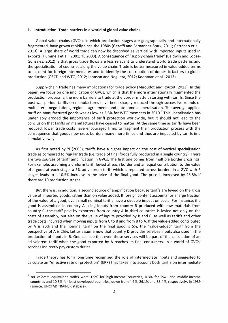
THE CUMULATIVE IMPACT OF TRADE BARRIERS ALONG THE VALUE CHAIN:

AN EMPIRICAL ASSESSMENT USING THE OECD INTER-COUNTRY INPUT-OUTPUT MODEL

Dorothée Rouzet and Sébastien Miroudot1

June 2013

Abstract Since the post-war period, tariffs on manufactures have been deeply reduced through successive rounds of multilateral negotiations, regional agreements and autonomous liberalisation. In addition, more recent trade agreements have addressed an increasing number of regulatory barriers to trade, including on services. While overall trade has been liberalised for many products, this does not mean that barriers such as tariffs have ceased to matter. In a world characterised by global value chains, even small tariffs can have a significant impact on trade because of their cumulative effect. Not only are tariffs repeated when intermediate inputs are traded across borders multiple times, but also downstream firms face tariffs on the full value of their exports, including on their imported inputs and tariffs previously paid. Tariffs can add up to a significant level by the time the finished good reaches customers. Against this backdrop, the paper proposes an assessment of the cumulative impact of tariffs on exports of goods from OECD countries and key emerging economies, using the OECD Inter-Country Input-Output model. Effective rates of protection are calculated on the basis of value-added exports and taking into account the cumulative impact of barriers along the value chain.

JEL classification: F13, F14, F15

1 Organisation for Economic Co-Operation and Development (OECD), Trade and Agriculture Directorate.

Contact: sebastien.miroudot@oecd.org and dorothee.rouzet@oecd.org. The views expressed in this paper are those of the authors, and do not necessarily represent those of the OECD Secretariat or the member countries of the OECD.

2

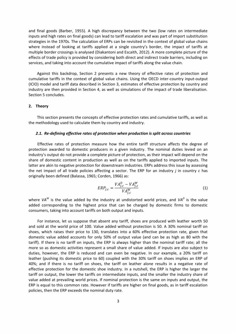
1. Introduction: Trade barriers in a world of global value chains

Global value chains (GVCs), in which production stages are geographically and internationally fragmented, have grown rapidly since the 1980s (Gereffi and Fernandez-Stark, 2011; Cattaneo et al., 2013). A large share of world trade can now be described as vertical with imported inputs used in exports (Hummels et al., 2001; Yi, 2003). A consequence of “supply-chain trade” (Baldwin and Lopez-Gonzales, 2012) is that gross trade flows are less relevant to understand world trade patterns and the specialisation of countries along the value chain. Trade is better measured in value-added terms to account for foreign intermediates and to identify the contribution of domestic factors to global production (OECD and WTO, 2012; Johnson and Noguera, 2012; Koopman et al., 2013).

Supply-chain trade has many implications for trade policy (Miroudot and Rouzet, 2013). In this

paper, we focus on one implication of GVCs, which is that the more internationally fragmented the production process is, the more barriers to trade at the border matter, starting with tariffs. Since the post-war period, tariffs on manufactures have been sharply reduced through successive rounds of multilateral negotiations, regional agreements and autonomous liberalisation. The average applied tariff on manufactured goods was as low as 2.6% for WTO members in 2010.2 This liberalisation has undeniably eroded the importance of tariff protection worldwide, but it should not lead to the conclusion that tariffs on manufactures have ceased to matter. At the same time as tariffs have been reduced, lower trade costs have encouraged firms to fragment their production process with the consequence that goods now cross borders many more times and thus are impacted by tariffs in a cumulative way.

As first noted by Yi (2003), tariffs have a higher impact on the cost of vertical specialisation

trade as compared to regular trade (i.e. trade of final foods fully produced in a single country). There are two sources of tariff amplification in GVCs. The first one comes from multiple border crossings. For example, assuming a uniform tariff levied at each border and an equal contribution to the value of a good at each stage, a 5% ad valorem tariff which is repeated across borders in a GVC with 5 stages leads to a 10.5% increase in the price of the final good. The price is increased by 25.8% if there are 10 production stages.

But there is, in addition, a second source of amplification because tariffs are levied on the gross

value of imported goods, rather than on value added. If foreign content accounts for a large fraction of the value of a good, even small nominal tariffs have a sizeable impact on costs. For instance, if a good is assembled in country A using inputs from country B produced with raw materials from country C, the tariff paid by exporters from country A in third countries is levied not only on the costs of assembly, but also on the value of inputs provided by B and C, as well as tariffs and other trade costs incurred when moving inputs from C to B and from B to A. If the value-added contributed by A is 20% and the nominal tariff on the final good is 5%, the “value-added” tariff from the perspective of A is 25%. Let us assume now that country D provides services inputs also used in the production of inputs in B. One can see that even these services will be part of the calculation of an ad valorem tariff when the good exported by A reaches its final consumers. In a world of GVCs, services indirectly pay custom duties.

Trade theory has for a long time recognised the role of intermediate inputs and suggested to

calculate an “effective rate of protection” (ERP) that takes into account both tariffs on intermediate

2 Ad valorem equivalent tariffs were 1.9% for high-income countries, 4.3% for low- and middle-income

countries and 10.3% for least developed countries, down from 4.6%, 26.1% and 88.4%, respectively, in 1989 (source: UNCTAD TRAINS database).

3

and final goods (Barber, 1955). A high discrepancy between the two (low rates on intermediate inputs and high rates on final goods) can lead to tariff escalation and was part of import substitution strategies in the 1970s. The calculation of ERPs can be revisited in the context of global value chains where instead of looking at tariffs applied at a single country’s border, the impact of tariffs at multiple border crossings is analysed (Diakantoni and Escaith, 2012). A more complete picture of the effects of trade policy is provided by considering both direct and indirect trade barriers, including on services, and taking into account the cumulative impact of tariffs along the value chain.

Against this backdrop, Section 2 presents a new theory of effective rates of protection and

cumulative tariffs in the context of global value chains. Using the OECD inter-country input-output (ICIO) model and tariff data described in Section 3, estimates of effective protection by country and industry are then provided in Section 4, as well as simulations of the impact of trade liberalisation. Section 5 concludes.

2. Theory

This section presents the concepts of effective protection rates and cumulative tariffs, as well as the methodology used to calculate them by country and industry.

2.1. Re-defining effective rates of protection when production is split across countries Effective rates of protection measure how the entire tariff structure affects the degree of

protection awarded to domestic producers in a given industry. The nominal duties levied on an industry’s output do not provide a complete picture of protection, as their impact will depend on the share of domestic content in production as well as on the tariffs applied to imported inputs. The latter are akin to negative protection for downstream industries. ERPs address this issue by assessing the net impact of all trade policies affecting a sector. The ERP for an industry j in country c has originally been defined (Balassa, 1965; Corden, 1966) as:

(1)

where VAW is the value added by the industry at undistorted world prices, and VAD is the value added corresponding to the highest price that can be charged by domestic firms to domestic consumers, taking into account tariffs on both output and inputs.

For instance, let us suppose that absent any tariff, shoes are produced with leather worth 50

and sold at the world price of 100. Value added without protection is 50. A 30% nominal tariff on shoes, which raises their price to 130, translates into a 60% effective protection rate, given that domestic value added accounts for only 50% of output value (and can be as high as 80 with the tariff). If there is no tariff on inputs, the ERP is always higher than the nominal tariff rate; all the more so as domestic activities represent a small share of value added. If inputs are also subject to duties, however, the ERP is reduced and can even be negative. In our example, a 20% tariff on leather (pushing its domestic price to 60) coupled with the 30% tariff on shoes implies an ERP of 40%; and if there is no tariff on shoes, the tariff on leather alone results in a negative rate of effective protection for the domestic shoe industry. In a nutshell, the ERP is higher the larger the tariff on output, the lower the tariffs on intermediate inputs, and the smaller the industry share of value added at prevailing world prices. If nominal protection is the same on inputs and output, the ERP is equal to this common rate. However if tariffs are higher on final goods, as in tariff escalation policies, then the ERP exceeds the nominal duty rate.

4

This concept takes a new meaning in a world characterised by global value chains, and newly available global input-output tables allow us to calculate it at an improved level of detail. As in Diakantoni and Escaith (2012), we can rewrite the ERP for sector j in country c as:

∑

∑ (2)

where tis,c is the nominal tariff rate applied to imports of industry i from country s to country c 3, tjW,c is the average nominal tariff on industry j output in country c (W stands for “world” as trade partner), and ais,jc is the value of sector i output from country s used in the production of one currency unit of sector j output in country c. The denominator is the share of sectoral value added, which includes the compensation of capital and labour used in production. The intermediate input shares ais,jc are elements of the matrix of technical coefficients A derived from the global inter-country input-output table. Assuming Leontief production functions, the ais,jc coefficients are exogenous. Under this assumption, equations (1) and (2) are equivalent.

The interpretation of ERPs is revisited in a GVC context. The concept was initially introduced as

a tool to describe and assess tariff escalation policies, by which the level of tariff protection increased with the degree of processing of the good, from low nominal duties on raw materials to high protection on finished products. A high ERP was then evidence that the country was pursuing such tariff escalation policies, designed to foster the development of domestic downstream sectors. Yet, while in the 1960s and 1970s a high ERP was part of import substitution strategies, the emphasis has now shifted to export competitiveness. What used to be a protectionist mix of policies to promote domestic industries has become an obstacle to a successful insertion into global markets characterised by vertical specialisation in GVCs. On the one hand, as before, tariffs on imported goods are harmful to the downstream industries that use those goods as inputs, and the magnitude of this effect has risen as not only primary commodities but also a vast range of intermediate inputs are traded across borders at every stage of the value chain. On the other hand, tariffs on a given industry’s output allow firms in this industry to sell at higher prices in their domestic market, but discourage exporting as exporters would have to compete at world prices. Besides, such tariffs raise the costs of other domestic firms further down in the value chain which purchase inputs – either domestically or abroad – from the protected industry, hampering their own export competitiveness. ERPs provide a tool to identify interdependencies between protective policies applied to different sectors and analyse the comprehensive effects of a country’s tariff policies on producers involved in global value chains.

A high ERP reveals a strong anti-export bias of trade policy, by which producers can charge

significantly higher prices on their domestic sales than on exports. Domestic tariff protection on their output is of no use for exporters trying to compete internationally either at world prices or facing protectionist policies in their export markets as well. High values of ERPs as measured in (2) discourage firms from exporting. It is therefore useful to distinguish effective protection for domestic sales and for exports. The effective rate of protection applying to exporters (without export taxes and export subsidies), noted ERPE, does not depend on the domestic tariff on their output but is affected by tariffs in destination countries:

∑

∑ (3)

3 Taking into account not only applied MFN tariffs but also, when allowed by data availability, preferential

treatment granted unilaterally or through preferential trade agreements.

5

where tjc,W is the average nominal tariff on imports from industry j in country c applied by its trade partners.

2.2. Calculating the cumulative cost of trade barriers along the value chain Calculating effective rates of protection, rather than looking at nominal rates, provides a more

comprehensive picture of the impact of the tariff environment on a given sector in a given country. Yet ERPs only take into account two stages of production – domestic producers and their imported inputs – but do not provide information on barriers further upstream and downstream.4 To this end, we calculate “cumulative tariffs” (CT) which instead of considering input and output protection at a specific stage of production, trace the total cost of all tariffs incurred along its production process. Taking into account the full structure of tariffs added up at all stages a good’s value chain will provide evidence on the extent to which trade costs are magnified in internationally fragmented production networks.

The cumulative tariffs embodied in an import of industry i from country s to country c has a

chain of components corresponding to backward production linkages. First, the direct tariff tis,c is incurred at the last border crossing. Second, industry i producers in country s have paid tariffs on their inputs from country c and third countries in proportion to their use of imported intermediate goods, which are given by the matrix of technical coefficients A. The sum of all second-stage tariffs is ∑ where subscripts k and u denote respectively the sectors and countries from which

industry i producers in country s source inputs. Each tariff is weighted by the share of the corresponding intermediate input in production, and domestically sourced inputs are assigned a zero tariff at this stage. Similarly, third-stage tariffs are given by ∑ . We can define in

a similar way fourth-stage tariffs, fifth-stage tariffs, and so on. Then, adding up custom duties levied at all stages, we obtain the cumulative tariff which has been paid on an import along its production chain, and we can compare it with the nominal tariff it faces on the last border crossing to assess the extent of tariff magnification.

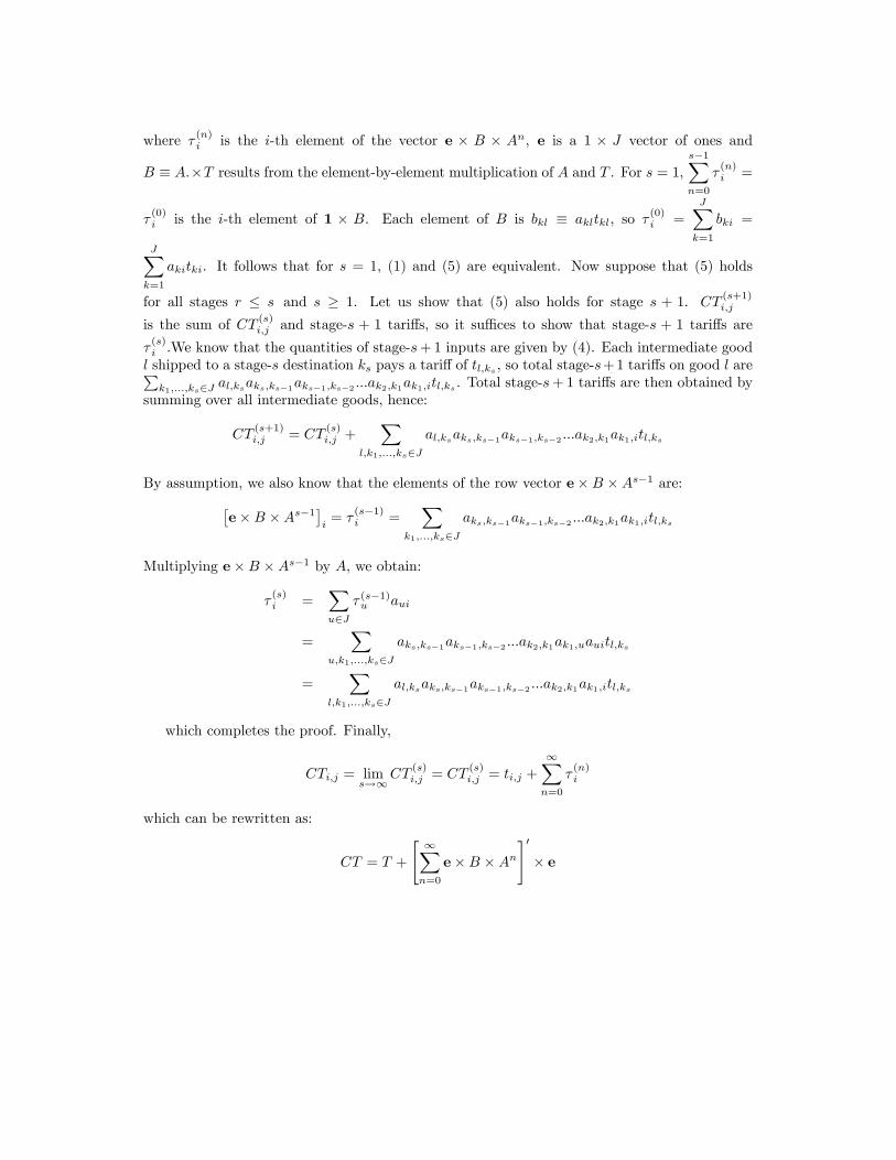
To simplify notation, let subscripts now denote a country-sector pair, so that aij is the

intermediate use of country-sector i output in country-sector j production, and tij is the nominal tariff per unit of import from i to j. tij is an element of the tariff matrix T and both A and T have dimensions J x J, where J is the number of country-sector observations. We can prove (see Annex 2) that the cumulative tariff on an import from country-sector i to country-sector j is:

∑

(4)

where

is the i-th element of the vector , is a 1 x J vector of ones and

results from the element-by-element multiplication of A and T. One measure of the magnification

effect is the ratio . Another one is the indirect tariff share ∑

.

4 Diakantoni and Escaith (2012) propose an alternative specification EPR" which incorporates the indirect

consumption of inputs using the Leontief coefficients instead of the technical coefficients in equation (2). However this formula implies that bilateral tariff rates are applied to trade flows that occurred indirectly and therefore were not subject to the imputed tariffs, but instead crossed borders several times possibly incurring tariffs several times and at different rates. This approach would therefore not allow us to reach conclusions on the effects of applied trade policies in internationally fragmented production processes.

6

3. Data

This section presents the two main sources of data used in the empirical exercise: trade flows and intermediate input use from the OECD input-output model, as well as data on applied tariffs.

3.1. The OECD Inter-Country Input-Output model Tracing trade barriers faced by a good along its production chain requires data on intermediate

input linkages between countries and industries. Our data source for international transactions at the industry level is the Inter-Country Input-Output (ICIO) model developed by the OECD. It was built from harmonised national input-output tables which are linked internationally with data on bilateral trade in goods by end-use category and bilateral trade in services, using only official sources. The methodology and assumptions underlying the construction of the OECD ICIO model are detailed in OECD-WTO (2012).

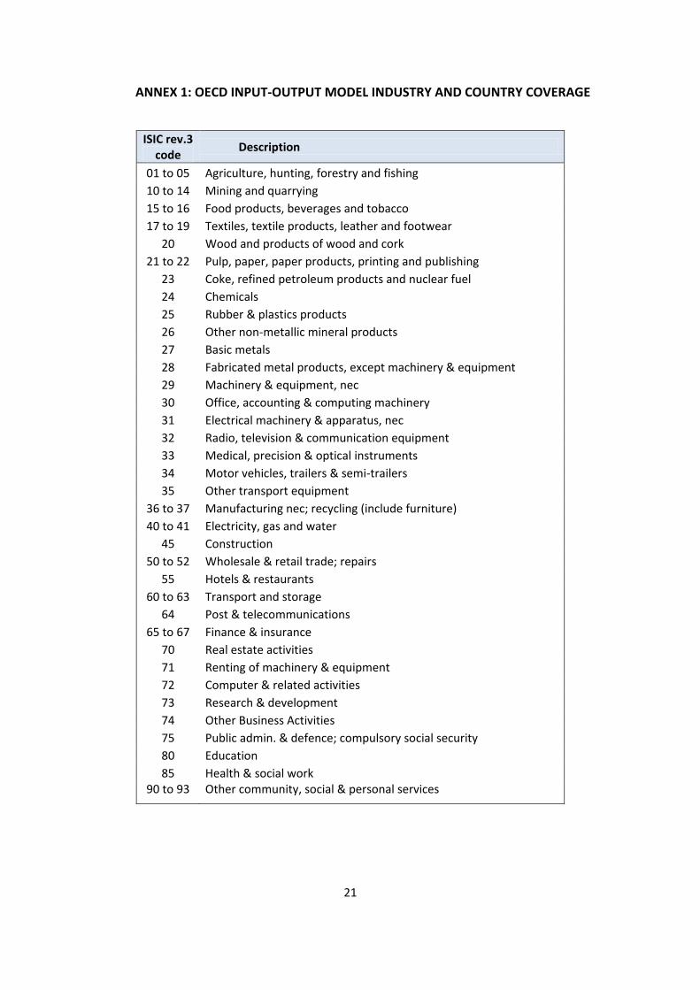
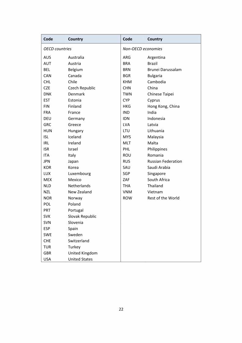
The resulting ICIO tables cover 57 economies and a “rest of the world” region, which account

for over 95% of world output, and 36 industries (Annex 1). They provide information on intermediate input use by purchasing industry, supplying industry, destination country and source country, as well as on value-added and gross output, thus enabling us to track the stages and locations of production along a sector’s value chain. The data are available for five years: 1995, 2000, 2005, 2008 and 2009. Our main estimates are for the most recent year (2009), and we also use 2005 as a comparison year. From global input-output tables, we derive the matrix A of technical coefficients. As explained above, an element of the matrix ais,jc is the value of sector i output from country s used as intermediate input in the production of 1 USD of sector j output in country c. Importantly, an underlying assumption of input-output models is that the structure of production is fixed following Leontief production functions. Therefore the results of our simulations with varying trade costs will best be interpreted as short-term estimates, before the impact of input substitution and general equilibrium effects.

3.2. Tariff rates by industry Tariff data is drawn from the UNCTAD-TRAINS database, which records tariffs and gross import

flows by country of origin for over 170 countries. The TRAINS database provides information on ad valorem equivalent tariffs at the disaggregated 6-digit level according to the Harmonized System (HS) nomenclature, by reporter and partner country. We use effectively applied tariffs (AHS) when available. If information on AHS tariffs is not reported for a given reporter-partner-product observation, we use preferential rates instead (PRF); although not exhaustive, the coverage of preferential tariffs in TRAINS include GSP preferences, other preferential rates granted to developing countries, regional trade agreements and a number of bilateral agreements. Finally if neither AHS nor PRF tariffs are available, we use applied Most Favoured Nation tariffs (MFN). Like the input-output data, our tariff data covers 2005 and 2009, or the closest available year if 2005 or 2009 is missing.

Tariffs are then aggregated for each country pair from the 6-digit HS level to the industry detail

of the OECD ICIO model, weighting each 6-digit product by its share of trade in the industry between the two countries as reported by the importer. For services imports, tariffs are zero between all countries. Economies not covered individually in the OECD ICIO data are aggregated into a “Rest of the world” region in the same manner. We obtain the matrix T of tariffs, where an element tis,jc is the tariff applied to direct imports of products from industry i in country s used by industry j in country c. Since tariffs on imported goods do not discriminate according to the industry of destination, tis,jc =

7

tis,kc for all j,k.5 The tariff matrix covers all country and sector pairs for the 58 economies and 36 industries in the OECD ICIO model.

4. Results

4.1. Effective rates of protection by country and industry We calculate effective rates of protection by country and industry according to equation (1).

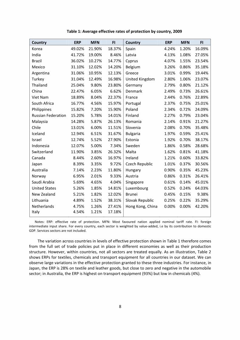
Table 1 shows the average ERP in goods sectors for each country in the dataset (sectors within a country are weighted by value-added), as well as the corresponding nominal MFN applied rates and shares of foreign intermediate inputs in output (FI). There are several factors determining the level of ERPs. First, higher nominal tariff rates directly raise the extent of effective protection: countries with the highest average MFN rates, such as Korea and India, are also those with the highest EPRs. However, our calculations also confirm that nominal tariffs are not the whole story. The manner in which a country’s tariff schedule affects its producers also depends on what they import, and how much value added is added by the sector itself in the production of its output. In particular, the increasing fragmentation of production tends to amplify the impact of tariffs.

For all countries, overall ERPs are higher than nominal MFN rates, for two reasons. On the one

hand, tariffs on raw materials and intermediate goods tend to be set lower than tariffs on processed and finished goods. On the other hand, the mere fact that a sector uses intermediate inputs, be they domestic or foreign, amplifies the impact of a given tariff when we measure protection relative to value-added rather than output, through the denominator in the definition of the ERP. This effect captures the fact that the degree of protection awarded to a sector, for a given nominal tariff imposed on its foreign counterparts, is higher when the domestic producer contributes a small share of the total value added of its output. For instance if value-added in the sector accounts for 50% of the total value of its output, a 10% tariff on output (without any input tariff) would imply that the domestic producer’s own labour and capital expenditures could be as much as 20% higher than those of foreign producers and it would still be charging lower prices in the domestic market.

This “value-added effect” explains, in particular, the high rate of effective protection in China

compared to nominal MFN protection. China has the lowest average shares of sectoral value-added in production, around 32%. By way of comparison, Thailand has higher nominal tariffs than China, but a similar average ERP. This comes both from higher shares of value-added by its industries (over 40% of the value of output, on average, is sectoral value-added in Thailand), and from a more intensive use of foreign intermediate inputs. As foreign inputs account for 24% of the value of output, trade costs on imported inputs erode the protection offered by the trade policy environment to downstream sectors. However it must be kept in mind that foreign inputs are subject to tariffs only outside of special economic zones, from which a significant share ofThailand’s exports originate. Another interesting comparison is between the European Union (EU) and other large developed economies such as the United States and Japan. EU countries have low nominal tariff rates as a large share of their imports is intra-EU, which contributes to low effective protection. They also use imported intermediate inputs more intensively (as shown by larger FI shares), but most of these imported inputs are sourced tariff-free from within the EU as well, which makes them similar to domestic inputs in terms of effective protection.

5 One caveat is that we do not take into account tariff exemptions granted in export processing zones and

through inward and outward processing trade regimes. These regimes introduce a differential tariff treatment of imports depending on the sectors and the firms to which they are destined, as imported goods entering into the production of exports are not subject to import duties.

8

Table 1: Average effective rates of protection by country, 2009

Country ERP MFN FI Country ERP MFN FI

Korea 49.02% 21.90% 18.37% Spain 4.24% 1.20% 16.09%

India 41.72% 19.00% 8.46% Latvia 4.13% 1.08% 27.05%

Brazil 36.02% 10.27% 14.77% Cyprus 4.07% 1.55% 23.54%

Mexico 31.10% 12.02% 14.20% Belgium 3.26% 0.86% 35.18%

Argentina 31.06% 10.95% 12.13% Greece 3.01% 0.99% 19.44%

Turkey 31.04% 12.49% 16.98% United Kingdom 2.80% 1.06% 23.07%

Thailand 25.04% 9.80% 23.80% Germany 2.79% 0.80% 21.12%

China 22.47% 6.05% 6.62% Denmark 2.49% 0.73% 26.61%

Viet Nam 18.89% 8.04% 22.37% France 2.44% 0.76% 22.89%

South Africa 16.77% 4.56% 15.97% Portugal 2.37% 0.75% 25.01%

Philippines 15.82% 7.20% 15.90% Poland 2.34% 0.72% 24.09%

Russian Federation 15.20% 5.78% 14.01% Finland 2.27% 0.79% 23.04%

Malaysia 14.28% 5.87% 26.13% Romania 2.14% 0.91% 21.27%

Chile 13.01% 6.00% 11.51% Slovenia 2.08% 0.70% 35.48%

Iceland 12.94% 6.51% 31.67% Bulgaria 1.97% 0.59% 25.41%

Israel 12.74% 5.52% 27.90% Estonia 1.92% 0.70% 38.17%

Indonesia 12.07% 5.00% 7.34% Sweden 1.86% 0.58% 28.68%

Switzerland 11.90% 3.85% 26.32% Malta 1.62% 0.81% 41.18%

Canada 8.44% 2.60% 16.97% Ireland 1.21% 0.60% 33.82%

Japan 8.39% 3.35% 9.72% Czech Republic 1.01% 0.37% 30.56%

Australia 7.14% 2.23% 11.80% Hungary 0.90% 0.35% 45.23%

Norway 6.95% 2.01% 9.33% Austria 0.86% 0.31% 26.41%

Saudi Arabia 5.69% 4.65% 4.04% Singapore 0.61% 0.14% 45.01%

United States 5.26% 1.85% 14.81% Luxembourg 0.52% 0.24% 64.03%

New Zealand 5.21% 1.82% 12.02% Brunei 0.45% 0.15% 9.38%

Lithuania 4.89% 1.52% 38.31% Slovak Republic 0.25% 0.22% 35.29%

Netherlands 4.75% 1.26% 27.41% Hong Kong, China 0.00% 0.00% 42.20% Italy 4.54% 1.21% 17.18%

Notes: ERP: effective rate of protection. MFN: Most favoured nation applied nominal tariff rate. FI: foreign intermediate input share. For every country, each sector is weighted by value-added, i.e by its contribution to domestic GDP. Services sectors are not included.

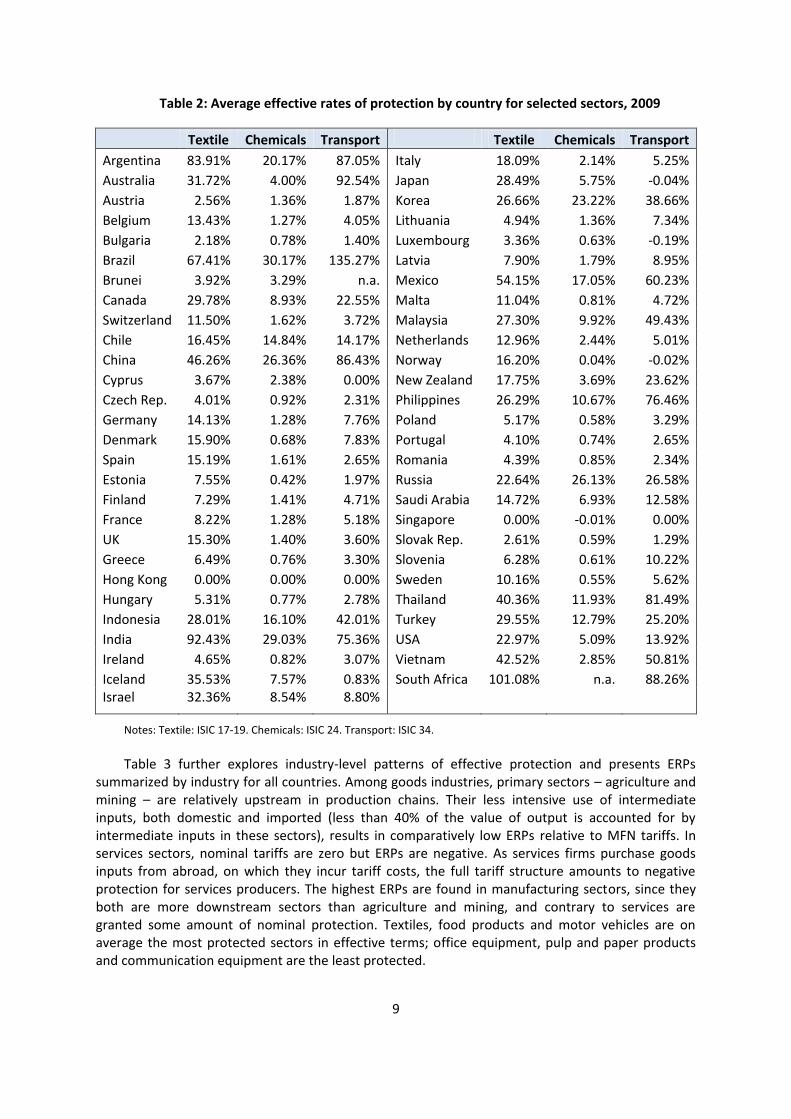
The variation across countries in levels of effective protection shown in Table 1 therefore comes

from the full set of trade policies put in place in different economies as well as their production structure. However, within countries, not all sectors are treated equally. As an illustration, Table 2 shows ERPs for textiles, chemicals and transport equipment for all countries in our dataset. We can observe large variations in the effective protection granted to these three industries. For instance, in Japan, the ERP is 28% on textile and leather goods, but close to zero and negative in the automobile sector; in Australia, the ERP is highest on transport equipment (93%) but low in chemicals (4%).

9

Table 2: Average effective rates of protection by country for selected sectors, 2009

Textile Chemicals Transport Textile Chemicals Transport

Argentina 83.91% 20.17% 87.05% Italy 18.09% 2.14% 5.25%

Australia 31.72% 4.00% 92.54% Japan 28.49% 5.75% -0.04%

Austria 2.56% 1.36% 1.87% Korea 26.66% 23.22% 38.66%

Belgium 13.43% 1.27% 4.05% Lithuania 4.94% 1.36% 7.34%

Bulgaria 2.18% 0.78% 1.40% Luxembourg 3.36% 0.63% -0.19%

Brazil 67.41% 30.17% 135.27% Latvia 7.90% 1.79% 8.95%

Brunei 3.92% 3.29% n.a. Mexico 54.15% 17.05% 60.23%

Canada 29.78% 8.93% 22.55% Malta 11.04% 0.81% 4.72%

Switzerland 11.50% 1.62% 3.72% Malaysia 27.30% 9.92% 49.43%

Chile 16.45% 14.84% 14.17% Netherlands 12.96% 2.44% 5.01%

China 46.26% 26.36% 86.43% Norway 16.20% 0.04% -0.02%

Cyprus 3.67% 2.38% 0.00% New Zealand 17.75% 3.69% 23.62%

Czech Rep. 4.01% 0.92% 2.31% Philippines 26.29% 10.67% 76.46%

Germany 14.13% 1.28% 7.76% Poland 5.17% 0.58% 3.29%

Denmark 15.90% 0.68% 7.83% Portugal 4.10% 0.74% 2.65%

Spain 15.19% 1.61% 2.65% Romania 4.39% 0.85% 2.34%

Estonia 7.55% 0.42% 1.97% Russia 22.64% 26.13% 26.58%

Finland 7.29% 1.41% 4.71% Saudi Arabia 14.72% 6.93% 12.58%

France 8.22% 1.28% 5.18% Singapore 0.00% -0.01% 0.00%

UK 15.30% 1.40% 3.60% Slovak Rep. 2.61% 0.59% 1.29%

Greece 6.49% 0.76% 3.30% Slovenia 6.28% 0.61% 10.22%

Hong Kong 0.00% 0.00% 0.00% Sweden 10.16% 0.55% 5.62%

Hungary 5.31% 0.77% 2.78% Thailand 40.36% 11.93% 81.49%

Indonesia 28.01% 16.10% 42.01% Turkey 29.55% 12.79% 25.20%

India 92.43% 29.03% 75.36% USA 22.97% 5.09% 13.92%

Ireland 4.65% 0.82% 3.07% Vietnam 42.52% 2.85% 50.81%

Iceland 35.53% 7.57% 0.83% South Africa 101.08% n.a. 88.26% Israel 32.36% 8.54% 8.80%

Notes: Textile: ISIC 17-19. Chemicals: ISIC 24. Transport: ISIC 34.

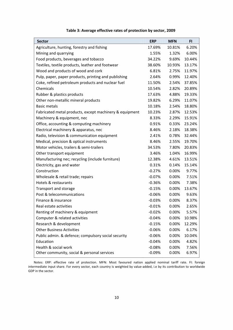
Table 3 further explores industry-level patterns of effective protection and presents ERPs

summarized by industry for all countries. Among goods industries, primary sectors – agriculture and mining – are relatively upstream in production chains. Their less intensive use of intermediate inputs, both domestic and imported (less than 40% of the value of output is accounted for by intermediate inputs in these sectors), results in comparatively low ERPs relative to MFN tariffs. In services sectors, nominal tariffs are zero but ERPs are negative. As services firms purchase goods inputs from abroad, on which they incur tariff costs, the full tariff structure amounts to negative protection for services producers. The highest ERPs are found in manufacturing sectors, since they both are more downstream sectors than agriculture and mining, and contrary to services are granted some amount of nominal protection. Textiles, food products and motor vehicles are on average the most protected sectors in effective terms; office equipment, pulp and paper products and communication equipment are the least protected.

10

Table 3: Average effective rates of protection by sector, 2009

Sector ERP MFN FI

Agriculture, hunting, forestry and fishing 17.69% 10.81% 6.20%

Mining and quarrying 1.55% 1.32% 6.00%

Food products, beverages and tobacco 34.22% 9.69% 10.44%

Textiles, textile products, leather and footwear 38.60% 10.93% 13.17%

Wood and products of wood and cork 6.81% 2.75% 11.97%

Pulp, paper, paper products, printing and publishing 2.64% 0.99% 12.40%

Coke, refined petroleum products and nuclear fuel 11.50% 2.54% 37.85%

Chemicals 10.54% 2.82% 20.89%

Rubber & plastics products 17.63% 4.88% 19.33%

Other non-metallic mineral products 19.82% 6.29% 11.07%

Basic metals 10.18% 2.54% 18.80%

Fabricated metal products, except machinery & equipment 10.23% 2.87% 12.53%

Machinery & equipment, nec 8.33% 2.29% 15.91%

Office, accounting & computing machinery 0.91% 0.33% 23.24%

Electrical machinery & apparatus, nec 8.46% 2.18% 18.38%

Radio, television & communication equipment 2.41% 0.78% 32.44%

Medical, precision & optical instruments 8.46% 2.55% 19.70%

Motor vehicles, trailers & semi-trailers 34.53% 7.80% 20.83%

Other transport equipment 3.46% 1.04% 16.99%

Manufacturing nec; recycling (include furniture) 12.38% 4.61% 13.51%

Electricity, gas and water 0.31% 0.14% 15.14%

Construction -0.27% 0.00% 9.77%

Wholesale & retail trade; repairs -0.07% 0.00% 7.51%

Hotels & restaurants -0.36% 0.00% 7.38%

Transport and storage -0.15% 0.00% 13.67%

Post & telecommunications -0.06% 0.00% 9.63%

Finance & insurance -0.03% 0.00% 8.37%

Real estate activities -0.01% 0.00% 2.65%

Renting of machinery & equipment -0.02% 0.00% 5.57%

Computer & related activities -0.04% 0.00% 10.98%

Research & development -0.15% 0.00% 12.29%

Other Business Activities -0.06% 0.00% 6.17%

Public admin. & defence; compulsory social security -0.06% 0.00% 10.04%

Education -0.04% 0.00% 4.82%

Health & social work -0.08% 0.00% 7.56% Other community, social & personal services -0.09% 0.00% 6.97%

Notes: ERP: effective rate of protection. MFN: Most favoured nation applied nominal tariff rate. FI: foreign intermediate input share. For every sector, each country is weighted by value-added, i.e by its contribution to worldwide GDP in the sector.

11

4.2. Cumulative tariffs and magnification effect Our second set of results estimates the magnification of trade costs due to multiple border

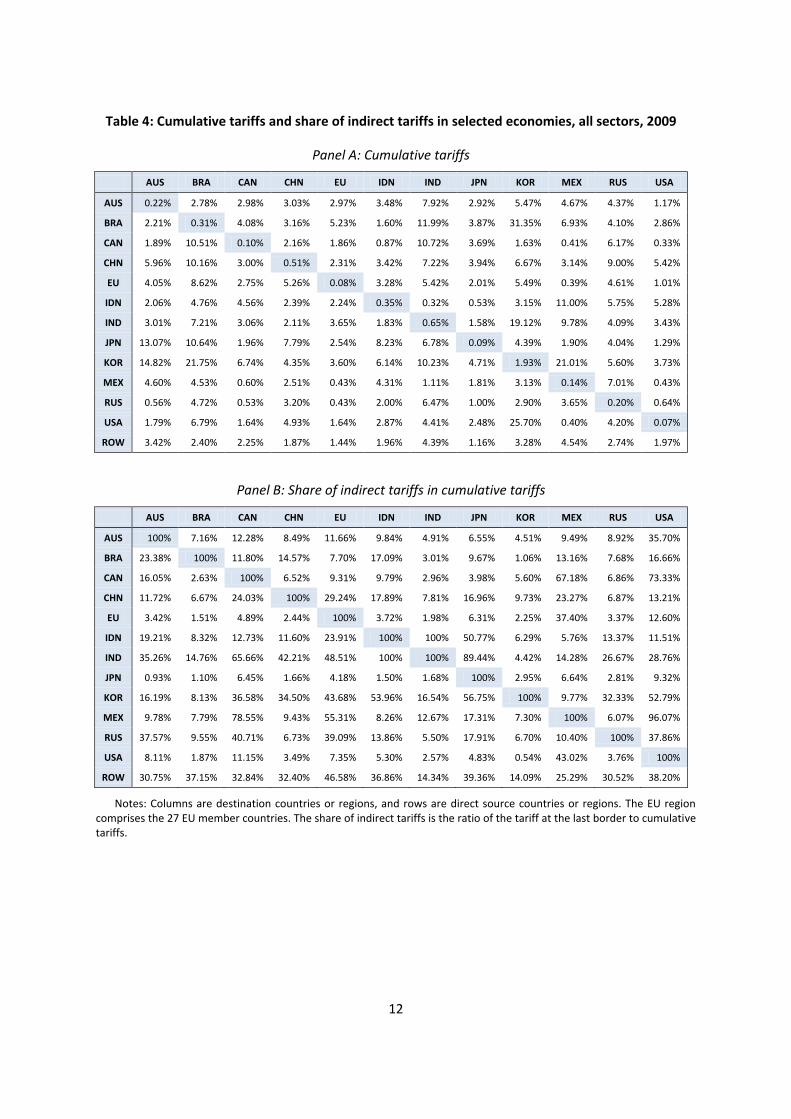
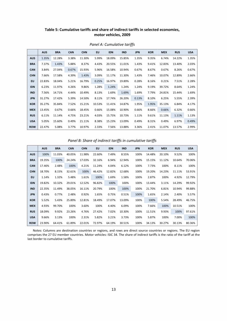
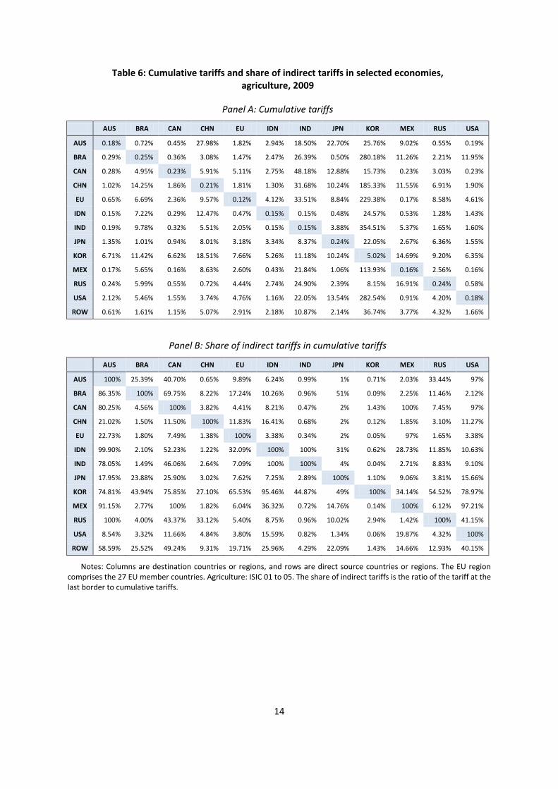
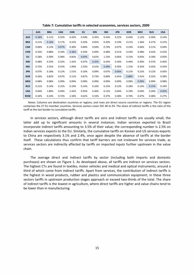
crossings along the value chain of a good or service. While ERPs look at a given stage in the value chain and how it is affected by trade policies put in place in the country where it is performed, cumulative tariffs (CTs) take the perspective of the whole value chain to add up the tariff costs that are paid on a good or service at all stages of its production process. We calculate it according to equation (4) for every destination country, direct source country and sector. Table 4 presents a summary matrix for all sectors combined and selected countries and regions. Columns are destination countries and rows are countries from which the good or service is purchased. Within countries and regions, CTs are weighted by the value of direct imports by the destination country from each country and sector (as intermediate inputs and for consumption by households or governments). This information is drawn from ICIO tables. Panel A shows cumulative tariffs. Panel B shows the share of CTs accounted for by indirect tariffs, i.e. by tariffs incurred before the last border crossing. For instance, goods and services imported from India into the EU pay an average total tariff of 3.65% (Panel A), 51.5% of which is directly levied at the India-EU border and 48.5% of which was paid on inputs imported into India and at previous production stages (Panel B). Tables 5, 6 and 7 show the same calculations for motor vehicles, agriculture and services. As there are no direct tariffs on services imports, the indirect tariff share (not shown) is 100% for all entries in Table 7.

Broadly speaking, CT estimates reveal that although nominal tariffs are low in most economies

at any given stage, indirect tariffs can add a significant burden by the time a good reaches its final user. Even within free-trade agreements, imports are not entirely tariff-free as they incorporate inputs from third countries that have been subject to tariffs. Canadian imports from the US, for instance, had on average been subject to a 1.6% tariff along their production process. Domestic purchases embody tariffs as well when we take a cumulative tariff perspective. The CT on domestic goods and services in Korea is 1.9% overall, and 5% in agriculture; several other countries (Australia, Brazil, China, Indonesia, India, Russia) have CTs in excess of 1% on domestic transactions in the motor vehicles industry.

The indirect and cumulative tariffs presented in Tables 4 to 7 focus on large developed and

emerging economies as destinations and direct sources. It should be kept in mind that these are precisely the countries that tend to have low nominal tariffs on manufacturing products and a larger share of value added produced domestically than small and developing economies. Therefore, the magnitude of the amplification effect of tariffs reported here can be interpreted as a conservative estimate. The cumulative trade-reducing impact of tariff barriers in global value chains is likely to be even more acute in less developed economies. Unfortunately, the scarcity of data on input-output linkages in developing countries does not allow us to conduct a systematic comparison of this tariff amplification effect in economies at different stages of development.

12

Table 4: Cumulative tariffs and share of indirect tariffs in selected economies, all sectors, 2009

Panel A: Cumulative tariffs

AUS BRA CAN CHN EU IDN IND JPN KOR MEX RUS USA

AUS 0.22% 2.78% 2.98% 3.03% 2.97% 3.48% 7.92% 2.92% 5.47% 4.67% 4.37% 1.17%

BRA 2.21% 0.31% 4.08% 3.16% 5.23% 1.60% 11.99% 3.87% 31.35% 6.93% 4.10% 2.86%

CAN 1.89% 10.51% 0.10% 2.16% 1.86% 0.87% 10.72% 3.69% 1.63% 0.41% 6.17% 0.33%

CHN 5.96% 10.16% 3.00% 0.51% 2.31% 3.42% 7.22% 3.94% 6.67% 3.14% 9.00% 5.42%

EU 4.05% 8.62% 2.75% 5.26% 0.08% 3.28% 5.42% 2.01% 5.49% 0.39% 4.61% 1.01%

IDN 2.06% 4.76% 4.56% 2.39% 2.24% 0.35% 0.32% 0.53% 3.15% 11.00% 5.75% 5.28%

IND 3.01% 7.21% 3.06% 2.11% 3.65% 1.83% 0.65% 1.58% 19.12% 9.78% 4.09% 3.43%

JPN 13.07% 10.64% 1.96% 7.79% 2.54% 8.23% 6.78% 0.09% 4.39% 1.90% 4.04% 1.29%

KOR 14.82% 21.75% 6.74% 4.35% 3.60% 6.14% 10.23% 4.71% 1.93% 21.01% 5.60% 3.73%

MEX 4.60% 4.53% 0.60% 2.51% 0.43% 4.31% 1.11% 1.81% 3.13% 0.14% 7.01% 0.43%

RUS 0.56% 4.72% 0.53% 3.20% 0.43% 2.00% 6.47% 1.00% 2.90% 3.65% 0.20% 0.64%

USA 1.79% 6.79% 1.64% 4.93% 1.64% 2.87% 4.41% 2.48% 25.70% 0.40% 4.20% 0.07%

ROW 3.42% 2.40% 2.25% 1.87% 1.44% 1.96% 4.39% 1.16% 3.28% 4.54% 2.74% 1.97%

Panel B: Share of indirect tariffs in cumulative tariffs

AUS BRA CAN CHN EU IDN IND JPN KOR MEX RUS USA

AUS 100% 7.16% 12.28% 8.49% 11.66% 9.84% 4.91% 6.55% 4.51% 9.49% 8.92% 35.70%

BRA 23.38% 100% 11.80% 14.57% 7.70% 17.09% 3.01% 9.67% 1.06% 13.16% 7.68% 16.66%

CAN 16.05% 2.63% 100% 6.52% 9.31% 9.79% 2.96% 3.98% 5.60% 67.18% 6.86% 73.33%

CHN 11.72% 6.67% 24.03% 100% 29.24% 17.89% 7.81% 16.96% 9.73% 23.27% 6.87% 13.21%

EU 3.42% 1.51% 4.89% 2.44% 100% 3.72% 1.98% 6.31% 2.25% 37.40% 3.37% 12.60%

IDN 19.21% 8.32% 12.73% 11.60% 23.91% 100% 100% 50.77% 6.29% 5.76% 13.37% 11.51%

IND 35.26% 14.76% 65.66% 42.21% 48.51% 100% 100% 89.44% 4.42% 14.28% 26.67% 28.76%

JPN 0.93% 1.10% 6.45% 1.66% 4.18% 1.50% 1.68% 100% 2.95% 6.64% 2.81% 9.32%

KOR 16.19% 8.13% 36.58% 34.50% 43.68% 53.96% 16.54% 56.75% 100% 9.77% 32.33% 52.79%

MEX 9.78% 7.79% 78.55% 9.43% 55.31% 8.26% 12.67% 17.31% 7.30% 100% 6.07% 96.07%

RUS 37.57% 9.55% 40.71% 6.73% 39.09% 13.86% 5.50% 17.91% 6.70% 10.40% 100% 37.86%

USA 8.11% 1.87% 11.15% 3.49% 7.35% 5.30% 2.57% 4.83% 0.54% 43.02% 3.76% 100%

ROW 30.75% 37.15% 32.84% 32.40% 46.58% 36.86% 14.34% 39.36% 14.09% 25.29% 30.52% 38.20%

Notes: Columns are destination countries or regions, and rows are direct source countries or regions. The EU region comprises the 27 EU member countries. The share of indirect tariffs is the ratio of the tariff at the last border to cumulative tariffs.

13

Table 5: Cumulative tariffs and share of indirect tariffs in selected economies, motor vehicles, 2009

Panel A: Cumulative tariffs

AUS BRA CAN CHN EU IDN IND JPN KOR MEX RUS USA

AUS 1.35% 12.28% 3.38% 11.30% 5.99% 18.09% 15.85% 1.35% 9.35% 6.74% 14.22% 1.35%

BRA 7.37% 1.43% 5.88% 8.37% 4.43% 20.55% 11.01% 1.43% 9.41% 12.83% 13.40% 2.03%

CAN 3.84% 27.04% 0.67% 15.93% 5.96% 16.58% 10.94% 0.67% 8.67% 0.67% 8.26% 0.67%

CHN 7.66% 17.58% 4.39% 1.43% 3.09% 11.17% 11.30% 1.43% 7.46% 10.07% 12.89% 2.66%

EU 22.83% 18.04% 5.21% 16.79% 0.25% 16.97% 19.89% 0.28% 8.16% 0.21% 7.51% 2.28%

IDN 6.23% 11.97% 4.26% 9.86% 1.28% 1.24% 1.24% 1.24% 9.19% 39.72% 8.64% 1.24%

IND 7.56% 14.71% 4.44% 10.49% 8.13% 1.69% 1.69% 1.69% 7.79% 24.81% 15.44% 1.69%

JPN 31.27% 17.42% 5.39% 14.50% 8.11% 17.74% 26.20% 0.13% 8.10% 6.25% 5.55% 2.39%

KOR 35.27% 35.84% 7.52% 15.21% 10.53% 11.41% 14.87% 1.95% 1.95% 35.13% 6.84% 4.17%

MEX 13.45% 0.67% 0.66% 18.45% 0.66% 15.08% 10.90% 0.66% 8.66% 0.66% 6.32% 0.66%

RUS 6.11% 11.14% 4.75% 23.21% 4.03% 15.75% 10.73% 1.11% 9.61% 11.13% 1.11% 1.13%

USA 5.05% 15.60% 0.49% 21.11% 8.38% 15.23% 13.09% 0.49% 8.31% 0.49% 6.97% 0.49%

ROW 22.47% 5.08% 3.77% 10.97% 2.33% 7.56% 13.88% 3.36% 2.41% 11.07% 13.57% 2.99%

Panel B: Share of indirect tariffs in cumulative tariffs

AUS BRA CAN CHN EU IDN IND JPN KOR MEX RUS USA

AUS 100% 11.03% 40.05% 11.98% 22.60% 7.49% 8.55% 100% 14.48% 20.10% 9.52% 100%

BRA 19.35% 100% 24.24% 17.03% 32.16% 6.94% 12.94% 100% 15.15% 11.12% 10.64% 70.06%

CAN 17.46% 2.48% 100% 4.21% 11.24% 4.04% 6.12% 100% 7.73% 100% 8.11% 100%

CHN 18.70% 8.15% 32.61% 100% 46.42% 12.82% 12.68% 100% 19.20% 14.23% 11.11% 53.91%

EU 1.14% 1.32% 5.48% 1.61% 100% 1.69% 1.58% 100% 2.87% 100% 4.92% 12.79%

IDN 19.82% 10.32% 29.01% 12.52% 96.82% 100% 100% 100% 13.44% 3.11% 14.29% 99.92%

IND 22.35% 11.49% 38.05% 16.11% 20.79% 100% 100% 100% 21.70% 6.81% 10.94% 99.88%

JPN 0.43% 0.77% 2.48% 0.92% 1.65% 0.75% 0.51% 100% 1.65% 2.14% 2.40% 5.57%

KOR 5.52% 5.43% 25.89% 12.81% 18.49% 17.07% 13.09% 100% 100% 5.54% 28.49% 46.75%

MEX 4.93% 99.70% 100% 3.60% 100% 4.40% 6.09% 100% 7.66% 100% 10.51% 100%

RUS 18.09% 9.92% 23.26% 4.76% 27.42% 7.02% 10.30% 100% 11.51% 9.93% 100% 97.61%

USA 9.66% 3.13% 100% 2.31% 5.82% 3.21% 3.73% 100% 5.87% 100% 7.00% 100%

ROW 23.90% 64.41% 61.89% 22.01% 72.97% 64.19% 30.51% 100% 34.13% 30.27% 30.13% 80.36%

Notes: Columns are destination countries or regions, and rows are direct source countries or regions. The EU region comprises the 27 EU member countries. Motor vehicles: ISIC 34. The share of indirect tariffs is the ratio of the tariff at the last border to cumulative tariffs.

14

Table 6: Cumulative tariffs and share of indirect tariffs in selected economies, agriculture, 2009

Panel A: Cumulative tariffs

AUS BRA CAN CHN EU IDN IND JPN KOR MEX RUS USA

AUS 0.18% 0.72% 0.45% 27.98% 1.82% 2.94% 18.50% 22.70% 25.76% 9.02% 0.55% 0.19%

BRA 0.29% 0.25% 0.36% 3.08% 1.47% 2.47% 26.39% 0.50% 280.18% 11.26% 2.21% 11.95%

CAN 0.28% 4.95% 0.23% 5.91% 5.11% 2.75% 48.18% 12.88% 15.73% 0.23% 3.03% 0.23%

CHN 1.02% 14.25% 1.86% 0.21% 1.81% 1.30% 31.68% 10.24% 185.33% 11.55% 6.91% 1.90%

EU 0.65% 6.69% 2.36% 9.57% 0.12% 4.12% 33.51% 8.84% 229.38% 0.17% 8.58% 4.61%

IDN 0.15% 7.22% 0.29% 12.47% 0.47% 0.15% 0.15% 0.48% 24.57% 0.53% 1.28% 1.43%

IND 0.19% 9.78% 0.32% 5.51% 2.05% 0.15% 0.15% 3.88% 354.51% 5.37% 1.65% 1.60%

JPN 1.35% 1.01% 0.94% 8.01% 3.18% 3.34% 8.37% 0.24% 22.05% 2.67% 6.36% 1.55%

KOR 6.71% 11.42% 6.62% 18.51% 7.66% 5.26% 11.18% 10.24% 5.02% 14.69% 9.20% 6.35%

MEX 0.17% 5.65% 0.16% 8.63% 2.60% 0.43% 21.84% 1.06% 113.93% 0.16% 2.56% 0.16%

RUS 0.24% 5.99% 0.55% 0.72% 4.44% 2.74% 24.90% 2.39% 8.15% 16.91% 0.24% 0.58%

USA 2.12% 5.46% 1.55% 3.74% 4.76% 1.16% 22.05% 13.54% 282.54% 0.91% 4.20% 0.18%

ROW 0.61% 1.61% 1.15% 5.07% 2.91% 2.18% 10.87% 2.14% 36.74% 3.77% 4.32% 1.66%

Panel B: Share of indirect tariffs in cumulative tariffs

AUS BRA CAN CHN EU IDN IND JPN KOR MEX RUS USA

AUS 100% 25.39% 40.70% 0.65% 9.89% 6.24% 0.99% 1% 0.71% 2.03% 33.44% 97%

BRA 86.35% 100% 69.75% 8.22% 17.24% 10.26% 0.96% 51% 0.09% 2.25% 11.46% 2.12%

CAN 80.25% 4.56% 100% 3.82% 4.41% 8.21% 0.47% 2% 1.43% 100% 7.45% 97%

CHN 21.02% 1.50% 11.50% 100% 11.83% 16.41% 0.68% 2% 0.12% 1.85% 3.10% 11.27%

EU 22.73% 1.80% 7.49% 1.38% 100% 3.38% 0.34% 2% 0.05% 97% 1.65% 3.38%

IDN 99.90% 2.10% 52.23% 1.22% 32.09% 100% 100% 31% 0.62% 28.73% 11.85% 10.63%

IND 78.05% 1.49% 46.06% 2.64% 7.09% 100% 100% 4% 0.04% 2.71% 8.83% 9.10%

JPN 17.95% 23.88% 25.90% 3.02% 7.62% 7.25% 2.89% 100% 1.10% 9.06% 3.81% 15.66%

KOR 74.81% 43.94% 75.85% 27.10% 65.53% 95.46% 44.87% 49% 100% 34.14% 54.52% 78.97%

MEX 91.15% 2.77% 100% 1.82% 6.04% 36.32% 0.72% 14.76% 0.14% 100% 6.12% 97.21%

RUS 100% 4.00% 43.37% 33.12% 5.40% 8.75% 0.96% 10.02% 2.94% 1.42% 100% 41.15%

USA 8.54% 3.32% 11.66% 4.84% 3.80% 15.59% 0.82% 1.34% 0.06% 19.87% 4.32% 100%

ROW 58.59% 25.52% 49.24% 9.31% 19.71% 25.96% 4.29% 22.09% 1.43% 14.66% 12.93% 40.15%

Notes: Columns are destination countries or regions, and rows are direct source countries or regions. The EU region comprises the 27 EU member countries. Agriculture: ISIC 01 to 05. The share of indirect tariffs is the ratio of the tariff at the last border to cumulative tariffs.

15

Table 7: Cumulative tariffs in selected economies, services sectors, 2009

AUS BRA CAN CHN EU IDN IND JPN KOR MEX RUS USA

AUS 0.18% 0.11% 0.32% 0.42% 0.59% 0.35% 0.43% 0.22% 0.44% 2.12% 0.30% 0.14%

BRA 0.21% 0.18% 0.17% 0.22% 0.20% 0.05% 0.20% 0.19% 0.21% 1.36% 0.27% 0.22%

CAN 0.06% 0.13% 0.07% 0.30% 0.84% 0.04% 0.74% 0.07% 0.24% 0.06% 0.11% 0.04%

CHN 0.33% 0.88% 0.34% 0.36% 0.34% 0.49% 0.48% 0.31% 0.54% 0.48% 0.42% 0.43%

EU 0.28% 0.39% 0.58% 0.82% 0.05% 0.62% 1.23% 0.06% 0.15% 0.05% 0.18% 0.05%

IDN 0.48% 0.33% 0.32% 1.42% 0.47% 0.35% 0.43% 0.34% 0.44% 0.30% 0.37% 0.46%

IND 0.75% 3.55% 0.55% 1.09% 2.53% 0.52% 0.49% 0.50% 1.15% 0.33% 0.45% 0.43%

JPN 0.07% 0.18% 0.12% 1.51% 0.16% 0.09% 0.07% 0.06% 0.12% 0.22% 0.12% 0.05%

KOR 0.56% 0.82% 0.67% 3.11% 0.87% 0.73% 0.68% 0.45% 0.88% 2.41% 0.32% 0.28%

MEX 0.08% 0.08% 0.09% 0.09% 0.09% 0.09% 0.09% 0.09% 0.09% 0.09% 0.09% 0.08%

RUS 0.21% 0.14% 0.15% 0.19% 0.14% 0.16% 0.15% 0.13% 0.18% 0.14% 0.15% 0.19%

USA 0.60% 1.89% 0.04% 2.42% 0.93% 0.36% 0.12% 0.04% 0.19% 0.04% 0.30% 0.05%

ROW 0.34% 0.24% 0.72% 2.34% 0.62% 0.33% 0.37% 0.38% 0.74% 0.47% 0.48% 0.27%

Notes: Columns are destination countries or regions, and rows are direct source countries or regions. The EU region comprises the 27 EU member countries. Services sectors cover ISIC 40 to 93. The share of indirect tariffs is the ratio of the tariff at the last border to cumulative tariffs.

In services sectors, although direct tariffs are zero and indirect tariffs are usually small, the

latter add up to significant amounts in several instances. Indian services exported to Brazil incorporate indirect tariffs amounting to 3.5% of their value; the corresponding number is 2.5% on Indian services exports to the EU. Similarly, the cumulative tariffs on Korean and US services exports to China are respectively 3.1% and 2.4%, once again despite the absence of tariffs at the border itself. These calculations thus confirm that tariff barriers are not irrelevant for services trade, as services sectors are indirectly affected by tariffs on imported inputs further upstream in the value chain.

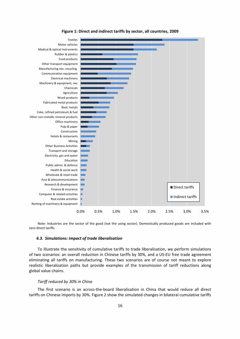
The average direct and indirect tariffs by sector (including both imports and domestic

purchases) are shown on Figure 1. As developed above, all tariffs are indirect on services sectors. The highest CTs are found in textiles, motor vehicles and medical and optical instruments, around a third of which come from indirect tariffs. Apart from services, the contribution of indirect tariffs is the highest in wood products, rubber and plastics and communication equipment; in these three sectors tariffs in upstream production stages approach or exceed two-thirds of the total. The share of indirect tariffs is the lowest in agriculture, where direct tariffs are higher and value chains tend to be lower than in manufacturing.

16

Figure 1: Direct and indirect tariffs by sector, all countries, 2009

Note: Industries are the sector of the good (not the using sector). Domestically produced goods are included with zero direct tariffs.

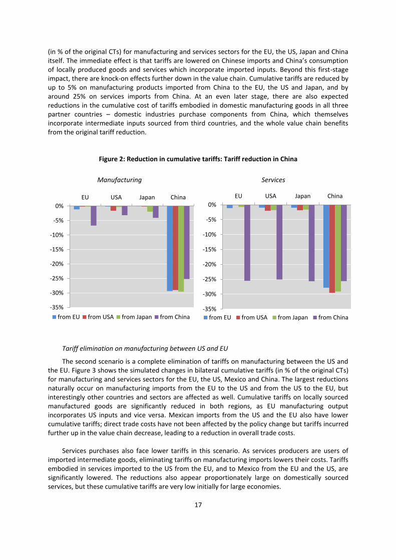
4.3. Simulations: impact of trade liberalisation To illustrate the sensitivity of cumulative tariffs to trade liberalisation, we perform simulations

of two scenarios: an overall reduction in Chinese tariffs by 30%, and a US-EU free trade agreement eliminating all tariffs on manufacturing. These two scenarios are of course not meant to explore realistic liberalization paths but provide examples of the transmission of tariff reductions along global value chains.

Tariff reduced by 30% in China

The first scenario is an across-the-board liberalisation in China that would reduce all direct tariffs on Chinese imports by 30%. Figure 2 show the simulated changes in bilateral cumulative tariffs

0.0% 0.5% 1.0% 1.5% 2.0% 2.5% 3.0% 3.5%

Renting of machinery & equipment

Real estate activities

Computer & related activities

Finance & insurance

Research & development

Post & telecommunications

Wholesale & retail trade

Health & social work

Public admin. & defence

Education

Electricity, gas and water

Transport and storage

Other Business Activities

Mining

Hotels & restaurants

Construction

Pulp & paper

Office machinery

Other non-metallic mineral products

Coke, refined petroleum & fuel

Basic metals

Fabricated metal products

Wood products

Agriculture

Chemicals

Machinery & equipment, nec

Electrical machinery

Communication equipment

Manufacturing nec; recycling

Other transport equipment

Food products

Rubber & plastics

Medical & optical instruments

Motor vehicles

Textiles

Direct tariffs

Indirect tariffs

17

(in % of the original CTs) for manufacturing and services sectors for the EU, the US, Japan and China itself. The immediate effect is that tariffs are lowered on Chinese imports and China’s consumption of locally produced goods and services which incorporate imported inputs. Beyond this first-stage impact, there are knock-on effects further down in the value chain. Cumulative tariffs are reduced by up to 5% on manufacturing products imported from China to the EU, the US and Japan, and by around 25% on services imports from China. At an even later stage, there are also expected reductions in the cumulative cost of tariffs embodied in domestic manufacturing goods in all three partner countries – domestic industries purchase components from China, which themselves incorporate intermediate inputs sourced from third countries, and the whole value chain benefits from the original tariff reduction.

Figure 2: Reduction in cumulative tariffs: Tariff reduction in China

Manufacturing

Services

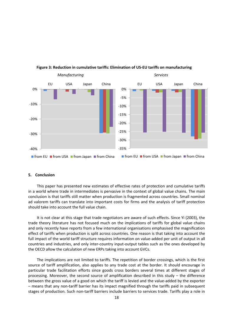
Tariff elimination on manufacturing between US and EU

The second scenario is a complete elimination of tariffs on manufacturing between the US and the EU. Figure 3 shows the simulated changes in bilateral cumulative tariffs (in % of the original CTs) for manufacturing and services sectors for the EU, the US, Mexico and China. The largest reductions naturally occur on manufacturing imports from the EU to the US and from the US to the EU, but interestingly other countries and sectors are affected as well. Cumulative tariffs on locally sourced manufactured goods are significantly reduced in both regions, as EU manufacturing output incorporates US inputs and vice versa. Mexican imports from the US and the EU also have lower cumulative tariffs; direct trade costs have not been affected by the policy change but tariffs incurred further up in the value chain decrease, leading to a reduction in overall trade costs.

Services purchases also face lower tariffs in this scenario. As services producers are users of

imported intermediate goods, eliminating tariffs on manufacturing imports lowers their costs. Tariffs embodied in services imported to the US from the EU, and to Mexico from the EU and the US, are significantly lowered. The reductions also appear proportionately large on domestically sourced services, but these cumulative tariffs are very low initially for large economies.

-35%

-30%

-25%

-20%

-15%

-10%

-5%

0%

EU USA Japan China

from EU from USA from Japan from China-35%

-30%

-25%

-20%

-15%

-10%

-5%

0%

EU USA Japan China

from EU from USA from Japan from China

18

Figure 3: Reduction in cumulative tariffs: Elimination of US-EU tariffs on manufacturing

Manufacturing

Services

5. Conclusion

This paper has presented new estimates of effective rates of protection and cumulative tariffs in a world where trade in intermediates is pervasive in the context of global value chains. The main conclusion is that tariffs still matter when production is fragmented across countries. Small nominal ad valorem tariffs can translate into important costs for firms and the analysis of tariff protection should take into account the full value chain.

It is not clear at this stage that trade negotiators are aware of such effects. Since Yi (2003), the

trade theory literature has not focused much on the implications of tariffs for global value chains and only recently have reports from a few international organisations emphasised the magnification effect of tariffs when production is split across countries. One reason is that taking into account the full impact of the world tariff structure requires information on value-added per unit of output in all countries and industries, and only inter-country input-output tables such as the ones developed by the OECD allow the calculation of new ERPs taking into account GVCs.

The implications are not limited to tariffs. The repetition of border crossings, which is the first

source of tariff amplification, also applies to any trade cost at the border. It should encourage in particular trade facilitation efforts since goods cross borders several times at different stages of processing. Moreover, the second source of amplification described in this study – the difference between the gross value of a good on which the tariff is levied and the value-added by the exporter – means that any non-tariff barrier has its impact magnified through the tariffs paid in subsequent stages of production. Such non-tariff barriers include barriers to services trade. Tariffs play a role in

-40%

-30%

-20%

-10%

0%

EU USA Japan China

from EU from USA from Japan from China

-35%

-30%

-25%

-20%

-15%

-10%

-5%

0%

EU USA Japan China

from EU from USA from Japan from China

19

trade in services as most services are inputs for manufacturing goods and indirectly incur the costs related to tariffs downstream. An estimation of the amplification effect of selected non-tariff measures in global value chains will be undertaken in future versions of this work.

The ERP is a partial equilibrium tool and the estimates presented in this paper do not indicate

to what extent welfare is affected and how changing tariff structures would impact production and consumption patterns. New models of trade where the supply chain is endogenously determined, such as Costinot et al. (2011) or Fally and Hillberry (2013), let us envisage such applications in the future. Such an approach would allow us to go beyond the assumption of a fixed production structure which underlies the construction of input-output tables, and to consider endogenous location choices as well as the elasticities of intermediate input demand and final consumption to trade costs.

Lastly, our estimates could be improved by taking into account processing regimes, duty

drawbacks and other schemes through which the exporter can avoid paying tariffs on its inputs. There is some evidence that such regimes play an important role in trade, not only in emerging economies such as China, but also for EU economies (Cernat and Pajot, 2012). There is, however, not enough information on the use of such regimes to incorporate them in the analysis. The estimates of protection rates presented are thus those for firms not benefiting from such schemes.

20

REFERENCES

Balassa, B. (1965), “Tariff Protection in Industrial Countries: An Evaluation”, Journal of Political

Economy 73(6), pp. 573-594.

Baldwin, R. and J. Lopez-Gonzalez (2012), “Supply-Chain Trade: A Portrait of Global Patterns and Several Testable Hypotheses”, mimeo.

Barber, C. (1955), “Canadian Tariff Policy”, Canadian Journal of Economics and Political Science 21(4), pp. 513-30.

Cattaneo, O., G. Gereffi, S. Miroudot and D. Taglioni (2013), “Joining, Upgrading and Being Competitive in Global Value Chains: A Strategic Framework”, World Bank Policy Research Working Paper No. 6406.

Cernat, L. and M. Pajot (2012), “ ‘Assembled in Europe’ – The role of processing trade in EU export performance”, Trade Chief Economist Note Issue 3/2012, European Commission.

Corden, W. M. (1966), “The Structure of a Tariff System and the Effective Protection Rate”, Journal of Political Economy 74(3), pp. 221-237.

Costinot, A., J. Vogel and S. Wang (2011), “An Elementary Theory of Global Supply Chains”, NBER Working Paper No. 16936.

Diakantoni, A. and H. Escaith (2012), “Reassessing Effective Protection Rates in a Trade in Tasks Perspective: Evolution of Trade Policy in ‘Factory Asia’”, MPRA Paper No. 41723.

Fally, T. and R. Hillberry (2013), “Quantifying Upstreamness in East Asia: Insights from a Coasian Model of Production Staging”, mimeo.

Gereffi, G. and K. Fernandez-Stark (2011), Global Value Chain Analysis: A Primer, Center on Globalization, Governance & Competitiveness (CGGC), Duke University, Durham, NC.

Hummels, D., J. Ishii and K.-M. Yi (2001), “The Nature and Growth of Vertical Specialization in World Trade”, Journal of International Economics 54(1), pp. 75-96.

Johnson, R.C. and G. Noguera (2012), “Accounting for Intermediates: Production Sharing and Trade in Value Added”, Journal of International Economics 86(2), pp. 224-236.

Koopman, R., Z. Wang and S.J. Wei (2013), “Tracing Value-Added and Double Counting in Gross Exports”, American Economic Review, forthcoming.

Miroudot, S. and D. Rouzet (2013), “Implications of Global Value Chains on Trade Policy”. In: Organisation for Economic Co-operation and Development, Interconnected economies: benefiting from global value chains, OECD Publishing, 2013, forthcoming.

Organisation for Economic Co-operation and Development and World Trade Organization (2012), “Trade in Value-Added: Concepts, Methodologies and Challenges”, joint OECD-WTO note.

Yi, K.-M. (2003), “Can Vertical Specialization Explain the Growth of World Trade?”, Journal of Political Economy 111(1), pp. 52-102.

21

ANNEX 1: OECD INPUT-OUTPUT MODEL INDUSTRY AND COUNTRY COVERAGE

ISIC rev.3 code

Description

01 to 05 Agriculture, hunting, forestry and fishing

10 to 14 Mining and quarrying

15 to 16 Food products, beverages and tobacco

17 to 19 Textiles, textile products, leather and footwear

20 Wood and products of wood and cork

21 to 22 Pulp, paper, paper products, printing and publishing

23 Coke, refined petroleum products and nuclear fuel

24 Chemicals

25 Rubber & plastics products

26 Other non-metallic mineral products

27 Basic metals

28 Fabricated metal products, except machinery & equipment

29 Machinery & equipment, nec

30 Office, accounting & computing machinery

31 Electrical machinery & apparatus, nec

32 Radio, television & communication equipment

33 Medical, precision & optical instruments

34 Motor vehicles, trailers & semi-trailers

35 Other transport equipment

36 to 37 Manufacturing nec; recycling (include furniture)

40 to 41 Electricity, gas and water

45 Construction

50 to 52 Wholesale & retail trade; repairs

55 Hotels & restaurants

60 to 63 Transport and storage

64 Post & telecommunications

65 to 67 Finance & insurance

70 Real estate activities

71 Renting of machinery & equipment

72 Computer & related activities

73 Research & development

74 Other Business Activities

75 Public admin. & defence; compulsory social security

80 Education

85 Health & social work 90 to 93 Other community, social & personal services

22

Code Country Code Country

OECD countries Non-OECD economies

AUS Australia ARG Argentina

AUT Austria BRA Brazil

BEL Belgium BRN Brunei Darussalam

CAN Canada BGR Bulgaria

CHL Chile KHM Cambodia

CZE Czech Republic CHN China

DNK Denmark TWN Chinese Taipei

EST Estonia CYP Cyprus

FIN Finland HKG Hong Kong, China

FRA France IND India

DEU Germany IDN Indonesia

GRC Greece LVA Latvia

HUN Hungary LTU Lithuania

ISL Iceland MYS Malaysia

IRL Ireland MLT Malta

ISR Israel PHL Philippines

ITA Italy ROU Romania

JPN Japan RUS Russian Federation

KOR Korea SAU Saudi Arabia

LUX Luxembourg SGP Singapore

MEX Mexico ZAF South Africa

NLD Netherlands THA Thailand

NZL New Zealand VNM Vietnam

NOR Norway ROW Rest of the World

POL Poland

PRT Portugal

SVK Slovak Republic

SVN Slovenia

ESP Spain

SWE Sweden

CHE Switzerland

TUR Turkey

GBR United Kingdom

USA United States

ANNEX 2: CUMULATIVE TARIFF FORMULA

Suppose there are J country-sector pairs. Each element of J identi�es both a country andindustry of origin or destination. The cumulative tari¤s embodied in an import of good (i; j)from country-sector i to country-sector j has a chain of components corresponding to backwardproduction linkages.

� Stage 0: The direct tari¤ ti;j is imposed by j on i imports.

� Stage 1: The �rst-tier suppliers k each provide ak;i units of k inputs per unit of i output.

Stage-1 tari¤s are thereforeJXk=1

akitki. Let CT(s)i;j be the cumulative tari¤s on good (i; j)

up to stage s. We have:

CT(1)i;j = ti;j +

JXk=1

akitki (1)

� Stage 2: The second-tier suppliers l each provide al;k units of l inputds per unit of each k

output. Stage-2 tari¤s are thereforeJXl=1

JXk=1

akialktlk, and the cumulative tari¤s on good

(i; j) up to stage 2 are:

CT(2)i;j = ti;j +

JXk=1

akitki +JXl=1

JXk=1

akialktlk (2)

In general, let us �rst show by recursion that for every l 2 J the total inputs of good lrequired for the production of �nal good (i; j) at stage s � 1 are �(s)l;i de�ned by:

�(s)l;i �

Xk1;:::;ks�12J

al;ks�1aks�1;ks�2 :::ak2;k1ak1;i (3)

By the de�nition of ak:i , we know that (3) holds for stage s = 1. Now suppose (3) holds fora stage s. At stage s+ 1, each unit of good l require am;l intermediate inputs of good m, so theinputs required to produce stage-s intermediate goods are, for each m 2 J :

�(s+1)m;i =

Xl2J

am;l�(s)l;i

=Xl2J

24 Xk1;:::;ks�12J

am;lal;ks�1aks�1;ks�2 :::ak2;k1ak1;i

35=

Xk1;:::;ks�1;l2J

am;lal;ks�1aks�1;ks�2 :::ak2;k1ak1;i

With a change of notation we obtain:

�(s+1)l;i �

Xk1;:::;ks2J

al;ksaks;ks�1aks�1;ks�2 :::ak2;k1ak1;i (4)

Second, let us show that for s � 1, cumulative tari¤s on good (i; j) up to stage s are givenby:

CT(s)i;j = ti;j +

s�1Xn=0

�(n)i (5)

where � (n)i is the i-th element of the vector e � B � An, e is a 1 � J vector of ones and

B � A:�T results from the element-by-element multiplication of A and T . For s = 1,s�1Xn=0

�(n)i =

�(0)i is the i-th element of 1 � B. Each element of B is bkl � akltkl, so �

(0)i =

JXk=1

bki =

JXk=1

akitki. It follows that for s = 1, (1) and (5) are equivalent. Now suppose that (5) holds

for all stages r � s and s � 1. Let us show that (5) also holds for stage s + 1. CT (s+1)i;j

is the sum of CT (s)i;j and stage-s + 1 tari¤s, so it su¢ ces to show that stage-s + 1 tari¤s are

�(s)i .We know that the quantities of stage-s+1 inputs are given by (4). Each intermediate goodl shipped to a stage-s destination ks pays a tari¤ of tl;ks , so total stage-s+1 tari¤s on good l areP

k1;:::;ks2J al;ksaks;ks�1aks�1;ks�2 :::ak2;k1ak1;itl;ks . Total stage-s+ 1 tari¤s are then obtained bysumming over all intermediate goods, hence:

CT(s+1)i;j = CT

(s)i;j +

Xl;k1;:::;ks2J

al;ksaks;ks�1aks�1;ks�2 :::ak2;k1ak1;itl;ks

By assumption, we also know that the elements of the row vector e�B �As�1 are:�e�B �As�1

�i= �

(s�1)i =

Xk1;:::;ks2J

aks;ks�1aks�1;ks�2 :::ak2;k1ak1;itl;ks

Multiplying e�B �As�1 by A, we obtain:

�(s)i =

Xu2J

� (s�1)u aui

=X

u;k1;:::;ks2Jaks;ks�1aks�1;ks�2 :::ak2;k1ak1;uauitl;ks

=X

l;k1;:::;ks2Jal;ksaks;ks�1aks�1;ks�2 :::ak2;k1ak1;itl;ks

which completes the proof. Finally,

CTi;j = lims!1

CT(s)i;j = CT

(s)i;j = ti;j +

1Xn=0

�(n)i

which can be rewritten as:

CT = T +

" 1Xn=0

e�B �An#0� e