The type Iax supernova, SN 2015H: A white dwarf deflagrationcandidate

Magee, M., Kotak, R., Sim, S. A., Kromer, M., Rabinowitz, D., Smartt, S. J., ... Young, D. R. (2016). The type Iaxsupernova, SN 2015H: A white dwarf deflagration candidate. Astronomy and Astrophysics, 589, [A89]. DOI:10.1051/0004-6361/201528036

Published in:Astronomy and Astrophysics

Document Version:Publisher's PDF, also known as Version of record

Queen's University Belfast - Research Portal:Link to publication record in Queen's University Belfast Research Portal

Publisher rights© ESO 2016

General rightsCopyright for the publications made accessible via the Queen's University Belfast Research Portal is retained by the author(s) and / or othercopyright owners and it is a condition of accessing these publications that users recognise and abide by the legal requirements associatedwith these rights.

Take down policyThe Research Portal is Queen's institutional repository that provides access to Queen's research output. Every effort has been made toensure that content in the Research Portal does not infringe any person's rights, or applicable UK laws. If you discover content in theResearch Portal that you believe breaches copyright or violates any law, please contact openaccess@qub.ac.uk.

Download date:29. Jul. 2018

A&A 589, A89 (2016)DOI: 10.1051/0004-6361/201528036c© ESO 2016

Astronomy&Astrophysics

The type Iax supernova, SN 2015H

A white dwarf deflagration candidate

M. R. Magee1, R. Kotak1, S. A. Sim1, M. Kromer2, D. Rabinowitz3, S. J. Smartt1, C. Baltay3, H. C. Campbell4,T.-W. Chen5, M. Fink6, A. Gal-Yam7, L. Galbany8, 9, W. Hillebrandt10, C. Inserra1, E. Kankare1, L. Le Guillou11, 12,

J. D. Lyman13, K. Maguire1, R. Pakmor14, F. K. Röpke14, A. J. Ruiter15, 16, I. R. Seitenzahl15, 16, M. Sullivan17,S. Valenti18, and D. R. Young1

1 Astrophysics Research Centre, School of Mathematics and Physics, Queen’s University Belfast, Belfast, BT7 1NN, UKe-mail: mmagee37@qub.ac.uk

2 The Oskar Klein Centre & Department of Astronomy, Stockholm University, AlbaNova, 106 91 Stockholm Sweden3 Department of Physics, Yale University, New Haven, CT 06250-8121, USA4 Institute of Astronomy, University of Cambridge, Madingley Road, Cambridge CB3 0HA, UK5 Max-Planck-Institut für Extraterrestrische Physik, Giessenbachstraße 1, 85748 Garching, Germany6 Institut für Theoretische Physik und Astrophysik, Universität Würzburg, Emil- Fischer Straße 31, 97074 Würzburg, Germany7 Department of Particle Physics and Astrophysics, Weizmann Institute of Science, 76100 Rehovot, Israel8 Milenium Institute of Astrophysics, 7820436 Macul Santiago, Chile9 Departamento de Astronomía, Universidad de Chile, Camino El Observatorio 1515, Las Condes, Santiago, Chile

10 Max-Planck-Institut für Astrophysik, Karl-Schwarzschild-Str. 1, 85748 Garching bei München, Germany11 Sorbonne Universites, UPMC Univ. Paris 06, UMR 7585, LPNHE, 75005 Paris, France12 CNRS, UMR 7585, Laboratoire de Physique Nucléaire et des Hautes Énergies, 4 place Jussieu, 75005 Paris, France13 Department of Physics, University of Warwick, Coventry CV4 7AL, UK14 Heidelberger Institut für Theoretische Studien, Schloss-Wolfsbrunnenweg 35, 69118 Heidelberg, Germany15 Research School of Astronomy and Astrophysics, Australian National University, Canberra, ACT 2611, Australia16 ARC Centre of Excellence for All-Sky Astrophysics (CAASTRO), Australia17 Department of Physics and Astronomy, University of Southampton, Southampton, SO17 1BJ, UK18 Department of Physics, University of California, Davis, CA 95616, USA

Received 23 December 2015 / Accepted 14 March 2016

ABSTRACT

We present results based on observations of SN 2015H which belongs to the small group of objects similar to SN 2002cx, oth-erwise known as type Iax supernovae. The availability of deep pre-explosion imaging allowed us to place tight constraints on theexplosion epoch. Our observational campaign began approximately one day post-explosion, and extended over a period of about150 days post maximum light, making it one of the best observed objects of this class to date. We find a peak magnitude ofMr = −17.27 ± 0.07, and a (∆m15)r = 0.69 ± 0.04. Comparing our observations to synthetic spectra generated from simulationsof deflagrations of Chandrasekhar mass carbon-oxygen white dwarfs, we find reasonable agreement with models of weak deflagra-tions that result in the ejection of ∼0.2 M� of material containing ∼0.07 M� of 56Ni. The model light curve however, evolves morerapidly than observations, suggesting that a higher ejecta mass is to be favoured. Nevertheless, empirical modelling of the pseudo-bolometric light curve suggests that .0.6 M� of material was ejected, implying that the white dwarf is not completely disrupted, andthat a bound remnant is a likely outcome.

Key words. supernovae: general – supernovae: individual: SN 2015H

1. Introduction

The use of Type Ia supernovae (SNe Ia) as standardizablecandles and cosmological distance indicators (Perlmutter et al.1999; Riess et al. 1998) has meant that they are among thebest studied transient phenomena in the Universe. In spite ofthis however, identifying the nature of the underlying progen-itor system(s) remains a key challenge. While it is generallyagreed that SNe Ia result from the thermonuclear explosion ofa carbon-oxygen white dwarf (CO WD), the explosion mech-anism and scenarios leading to explosion remain unclear (e.g.Hillebrandt et al. 2013). During the course of transient surveys,some of which are dedicated to searching for SNe Ia, many

peculiar transients have been discovered. A small subset of theseshow similarities to SNe Ia, but also striking differences. If thesealso result from thermonuclear explosions, then they may proveto be an excellent opportunity to test the extreme boundaries ofexplosion models.

One such class of peculiar SNe Ia are the SN 2002cx-likeobjects, that have recently been dubbed “SNe Iax” (Li et al.2003; Foley et al. 2013). The first examples of this group in-cluded SN 2002cx which was immediately recognized as be-ing different from SNe Ia (Li et al. 2003). A few years later,it was followed by SN 2005hk (Phillips et al. 2007). Both ob-jects showed similarities to each other, but diverged from usualSNe Ia behaviour. A subsequent search yielded ∼25 objects that

Article published by EDP Sciences A89, page 1 of 18

A&A 589, A89 (2016)

were deemed to exhibit properties in common with SNe 2002cxand 2005hk (Foley et al. 2013). This sample contains some verywell observed SNe Iax such as SN 2012Z, for which thereis a pre-explosion point source coincident with the supernova(McCully et al. 2014a). However, it also necessarily includedsome objects with incomplete data sets. The main observationalproperties that link SNe Iax include slow expansion velocities –roughly half that of normal SNe Ia at similar epochs – spectrathat are dominated by intermediate mass (IME) and iron-groupelements (IGE; Li et al. 2003; Branch et al. 2004), and peak ab-solute brightnesses that span about five magnitudes (−14 &MV & −19; Li et al. 2003; Branch et al. 2004; Foley et al. 2009,2013).

Despite the fact that SNe Iax are generally sub-luminouscompared to normal1 SNe Ia, their early-time spectra (i.e., be-fore or around maximum light), are intriguingly similar to thoseof over-luminous SNe Ia such as SN 1991T (Filippenko et al.1992). Indeed, the prototypical member of the SN Iax class,SN 2002cx, exhibited features of Fe iii in pre-maximum spectra(Li et al. 2003), similar to SN 1991T-like objects (Li et al. 1999).Spectral features due to Si ii, S ii, and Ca ii, that are prominent inthe spectra of normal SNe Ia, have been shown to be present inSNe Iax (Branch et al. 2004). However, it is at later epochs still,that the differences between SNe Ia and the SNe Iax becomemost pronounced. While spectra of the former are dominated byforbidden emission lines of IGEs, spectra of the latter exhibita forest of permitted lines from IGEs. This may indicate thatthe ejecta density is higher compared to SNe Ia at comparableepochs (Sahu et al. 2008).

Given that SNe Iax differ markedly in their properties whencompared to SNe Ia, alternative explosion mechanisms, and/orprogenitor systems are probably necessary. A possible explo-sion model for SNe Iax that has been widely considered sincethe early discoveries is that of pure deflagrations of whitedwarfs (Branch et al. 2004; Phillips et al. 2007). These mod-els differ from contemporary explosion models proposed fornormal SNe Ia in that they do not involve a detonation phase(Hillebrandt & Niemeyer 2000). Deflagration models could nat-urally explain some of the observed aspects of SNe Iax such astheir lower kinetic energy and lower luminosity compared to nor-mal SNe Ia.

Indeed, synthetic observables obtained from deflagrationmodels presented by Fink et al. (2014), Kromer et al. (2013,2015), and Long et al. (2014) have shown broad agreement withSNe Iax observables at early times. Nevertheless, the models di-verge from observations at later times, indicating that we aremissing key pieces in the puzzle that are the SNe Iax. Alterna-tive models to pure deflagrations have also been proposed forSNe Iax; in particular Stritzinger et al. (2015) have shown goodagreement for a pulsational delayed detonation model with abright SN Iax, SN 2012Z. In the context of such models, therange in parameter space spanned by the observations may beattributed to variations in a combination of the details of the ig-nition as well as inherent diversity in the progenitor systems.It nevertheless remains to be seen whether a single class ofmodel is able to account for the full brightness range spannedby SNe Iax.

We also note in passing that non-thermonuclear explosionscenarios have also been invoked for SNe Iax, in particular, forSN 2008ha. The apparent similarities between SN 2008ha, andsome faint core-collapse (II-Plateau) SNe has led to suggestions

1 We use the term “normal” to indicate “Branch-normal” type Ia SNe(Branch et al. 1993).

EN

LCOGT-CPT r-band, +6 d

2`

12

3 98

76

54

10``

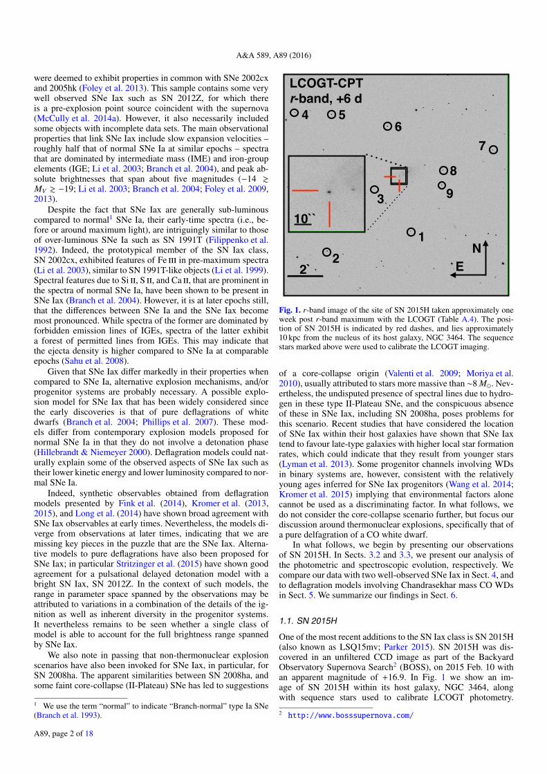
Fig. 1. r-band image of the site of SN 2015H taken approximately oneweek post r-band maximum with the LCOGT (Table A.4). The posi-tion of SN 2015H is indicated by red dashes, and lies approximately10 kpc from the nucleus of its host galaxy, NGC 3464. The sequencestars marked above were used to calibrate the LCOGT imaging.

of a core-collapse origin (Valenti et al. 2009; Moriya et al.2010), usually attributed to stars more massive than ∼8 M�. Nev-ertheless, the undisputed presence of spectral lines due to hydro-gen in these type II-Plateau SNe, and the conspicuous absenceof these in SNe Iax, including SN 2008ha, poses problems forthis scenario. Recent studies that have considered the locationof SNe Iax within their host galaxies have shown that SNe Iaxtend to favour late-type galaxies with higher local star formationrates, which could indicate that they result from younger stars(Lyman et al. 2013). Some progenitor channels involving WDsin binary systems are, however, consistent with the relativelyyoung ages inferred for SNe Iax progenitors (Wang et al. 2014;Kromer et al. 2015) implying that environmental factors alonecannot be used as a discriminating factor. In what follows, wedo not consider the core-collapse scenario further, but focus ourdiscussion around thermonuclear explosions, specifically that ofa pure delfagration of a CO white dwarf.

In what follows, we begin by presenting our observationsof SN 2015H. In Sects. 3.2 and 3.3, we present our analysis ofthe photometric and spectroscopic evolution, respectively. Wecompare our data with two well-observed SNe Iax in Sect. 4, andto deflagration models involving Chandrasekhar mass CO WDsin Sect. 5. We summarize our findings in Sect. 6.

1.1. SN 2015H

One of the most recent additions to the SN Iax class is SN 2015H(also known as LSQ15mv; Parker 2015). SN 2015H was dis-covered in an unfiltered CCD image as part of the BackyardObservatory Supernova Search2 (BOSS), on 2015 Feb. 10 withan apparent magnitude of +16.9. In Fig. 1 we show an im-age of SN 2015H within its host galaxy, NGC 3464, alongwith sequence stars used to calibrate LCOGT photometry.

2 http://www.bosssupernova.com/

A89, page 2 of 18

M. R. Magee et al.: SN 2015H

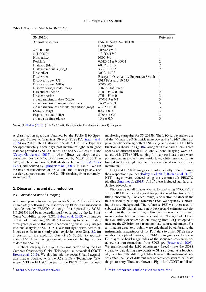
Table 1. Summary of details for SN 2015H.

SN 2015H ReferenceAlternative names PSN J10544216-2104138

LSQ15mvα (J2000.0) 10h54m42s.16 1δ (J2000.0) −21◦04′13′′.7 1Host galaxy NGC 3464 1Redshift 0.012462 ± 0.00001 2Distance (Mpc) 60.57 ± 1.95 2Distance modulus (mag) 33.91 ± 0.07 2Host offset 30′′E, 14′′ S 1Discoverer Backyard Observatory Supernova Search 1Discovery date (UT) 2015 February 10.545 1Discovery date (MJD) 57 064.05 1Discovery magnitude (mag) +16.9 (Unfiltered) 1Galactic extinction E(B − V) = 0.048 2Host extinction E(B − V) = 0 3r-band maximum date (MJD) 57 061.9 ± 0.4 3r-band maximum magnitude (mag) 16.77 ± 0.03 3r-band maximum absolute magnitude (mag) –17.27 ± 0.07 3(∆m15)r (mag) 0.69 ± 0.04 3Explosion date (MJD) 57 046 ± 0.5 3r-band rise time (days) 15.9 ± 0.6 3

Notes. (1) Parker (2015); (2) NASA/IPAC Extragalactic Database (NED); (3) this paper.

A classification spectrum obtained by the Public ESO Spec-troscopic Survey of Transient Objects (PESSTO, Smartt et al.2015) on 2015 Feb. 11 showed SN 2015H to be a Type IaxSN approximately a few days post-maximum light, with goodmatches provided by SN 2005cc at +5 d and SN 2002cx at +10 d(Zelaya-Garcia et al. 2015). In what follows, we adopt the dis-tance modulus for NGC 3464 provided by NED3 of 33.91 ±0.07, which is based on the Tully-Fisher relation (Tully & Fisher1977), and derived by Springob et al. (2009). In Table 1 we listthe basic characteristics of SN 2015H and its host galaxy, andour derived parameters for SN 2015H resulting from our analy-sis in Sect. 3.

2. Observations and data reduction

2.1. Optical and near-IR imaging

A follow-up monitoring campaign for SN 2015H was initiatedimmediately following the discovery by BOSS and subsequentclassification by PESSTO. Although first reported by BOSS,SN 2015H had been serendipitously observed by the La Silla-Quest Variability survey (LSQ, Baltay et al. 2013) with imagesof the field containing SN 2015H extending to approximatelythree years prior to this date. Incorporating these LSQ imagesinto our analysis of SN 2015H, our full light curve across allfilters extends from shortly after explosion (see Sect. 3.2 fordiscussion on the explosion date of SN 2015H) to approxi-mately 160 d later, making it one of the best sampled light curvesto date for SNe Iax.

Optical imaging in the gri filters was provided by the LasCumbres Observatory Global Telescope 1-m network (LCOGT,Brown et al. 2013). We also include the seven V-band acquisi-tion images obtained with the 3.58-m New Technology Tele-scope (NTT) + EFOSC2, as part of the PESSTO spectroscopic

3 http://ned.ipac.caltech.edu

monitoring campaign for SN 2015H. The LSQ survey makes useof the 40-inch ESO Schmidt telescope and a “wide” filter ap-proximately covering both the SDSS g- and r-bands. This filterfunction is shown in Fig. 10e, along with standard filters. Threeepochs of dithered near-IR J- and H-band imaging were ob-tained with NTT+SOFI, ranging from approximately one weekpost-maximum to over three weeks later, while time constraintslimited us to a single Ks-band observation at one week postmaximum.

LSQ and LCOGT images are automatically reduced usingtheir respective pipelines (Baltay et al. 2013; Brown et al. 2013).NTT images were reduced using the custom-built PESSTOpipeline Smartt et al. (2015). All of these included standard re-duction procedures.

Photometry on all images was performed using SNOoPY4, acustom IRAF package designed for point spread function (PSF)fitting photometry. For each image, a collection of stars in thefield is used to build up a reference PSF. We began by subtract-ing the sky background. The reference PSF was then used tosubtract the SN signal, and a new background estimate was de-rived from the residual image. This process was then repeatedin an iterative fashion to finally obtain the SN magnitude. Giventhe availability of pre-explosion imaging from LSQ, we opted tomeasure the SN brightness from template-subtracted images. Forall imaging data, zero points were calculated by calibrating theinstrumental magnitudes of the PSF stars to either SDSS mag-nitudes for optical images, or 2MASS magnitudes for near-IR images. V-band magnitudes of the sequence stars were ob-tained via transformations from SDSS gri (Jester et al. 2005).We transformed the LSQ photometry directly into the SDSSr-band by calculating zero points to SDSS r-band as a functionof g−r colour. The differing fields-of-view of the instruments ne-cessitated the use of different sets of sequence stars to calibratethe photometry. These are shown in Fig. 1 for LCOGT, and listed

4 http://sngroup.oapd.inaf.it/snoopy.html

A89, page 3 of 18

A&A 589, A89 (2016)

15

16

17

18

19

20

57040 57060 57080 57100 57120 57140 57160 57180 57200 57220

-20 0 20 40 60 80 100 120 140

Apparent Magnitude

MJD

Days since maximum

g + 1V + 0.5

ri - 0.5J - 1

H - 1.5K - 2

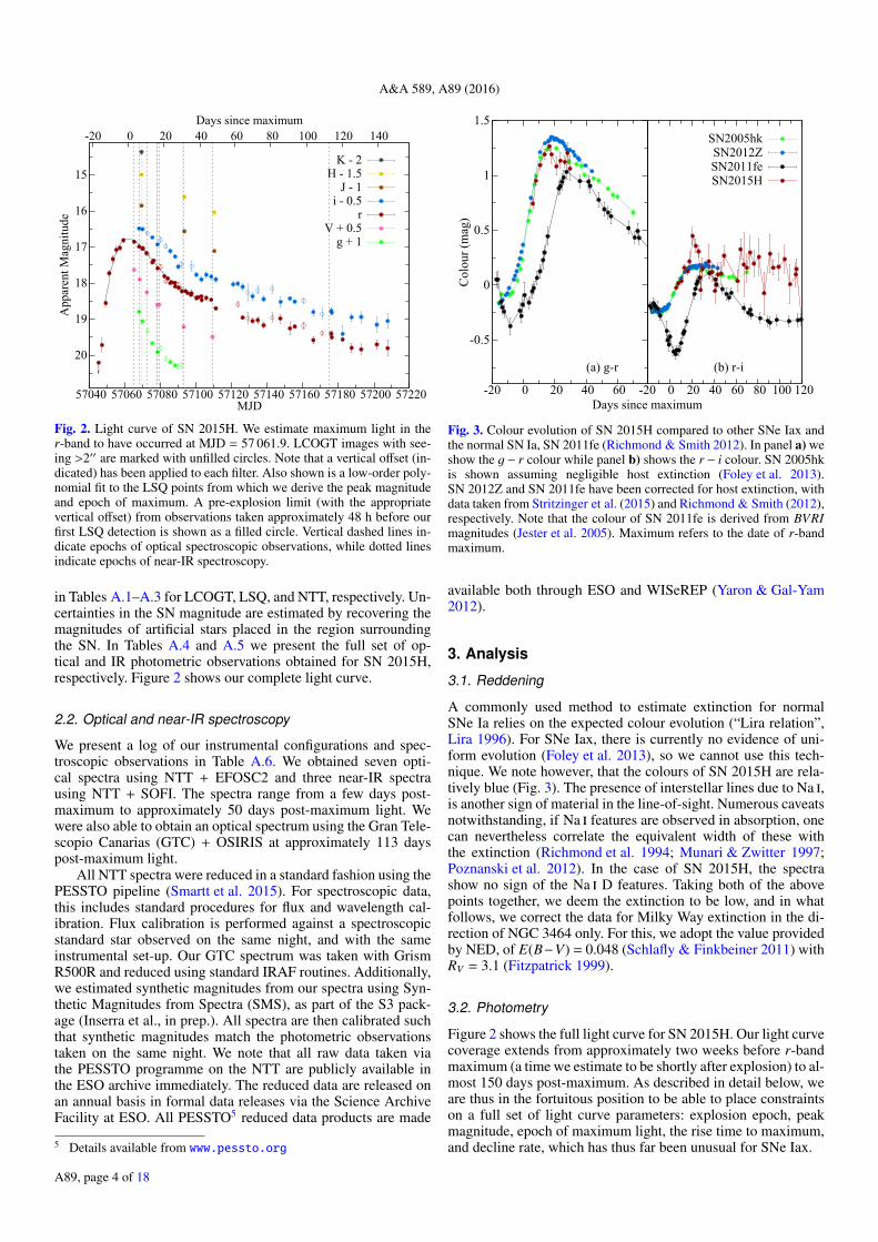
Fig. 2. Light curve of SN 2015H. We estimate maximum light in ther-band to have occurred at MJD = 57 061.9. LCOGT images with see-ing >2′′ are marked with unfilled circles. Note that a vertical offset (in-dicated) has been applied to each filter. Also shown is a low-order poly-nomial fit to the LSQ points from which we derive the peak magnitudeand epoch of maximum. A pre-explosion limit (with the appropriatevertical offset) from observations taken approximately 48 h before ourfirst LSQ detection is shown as a filled circle. Vertical dashed lines in-dicate epochs of optical spectroscopic observations, while dotted linesindicate epochs of near-IR spectroscopy.

in Tables A.1–A.3 for LCOGT, LSQ, and NTT, respectively. Un-certainties in the SN magnitude are estimated by recovering themagnitudes of artificial stars placed in the region surroundingthe SN. In Tables A.4 and A.5 we present the full set of op-tical and IR photometric observations obtained for SN 2015H,respectively. Figure 2 shows our complete light curve.

2.2. Optical and near-IR spectroscopy

We present a log of our instrumental configurations and spec-troscopic observations in Table A.6. We obtained seven opti-cal spectra using NTT + EFOSC2 and three near-IR spectrausing NTT + SOFI. The spectra range from a few days post-maximum to approximately 50 days post-maximum light. Wewere also able to obtain an optical spectrum using the Gran Tele-scopio Canarias (GTC) + OSIRIS at approximately 113 dayspost-maximum light.

All NTT spectra were reduced in a standard fashion using thePESSTO pipeline (Smartt et al. 2015). For spectroscopic data,this includes standard procedures for flux and wavelength cal-ibration. Flux calibration is performed against a spectroscopicstandard star observed on the same night, and with the sameinstrumental set-up. Our GTC spectrum was taken with GrismR500R and reduced using standard IRAF routines. Additionally,we estimated synthetic magnitudes from our spectra using Syn-thetic Magnitudes from Spectra (SMS), as part of the S3 pack-age (Inserra et al., in prep.). All spectra are then calibrated suchthat synthetic magnitudes match the photometric observationstaken on the same night. We note that all raw data taken viathe PESSTO programme on the NTT are publicly available inthe ESO archive immediately. The reduced data are released onan annual basis in formal data releases via the Science ArchiveFacility at ESO. All PESSTO5 reduced data products are made

5 Details available from www.pessto.org

-0.5

0

0.5

1

1.5

-20 0 20 40 60

(a) g-r

Colour (mag)

Days since maximum-20 0 20 40 60 80 100 120

(b) r-i

SN2005hkSN2012ZSN2011feSN2015H

Fig. 3. Colour evolution of SN 2015H compared to other SNe Iax andthe normal SN Ia, SN 2011fe (Richmond & Smith 2012). In panel a) weshow the g − r colour while panel b) shows the r − i colour. SN 2005hkis shown assuming negligible host extinction (Foley et al. 2013).SN 2012Z and SN 2011fe have been corrected for host extinction, withdata taken from Stritzinger et al. (2015) and Richmond & Smith (2012),respectively. Note that the colour of SN 2011fe is derived from BVRImagnitudes (Jester et al. 2005). Maximum refers to the date of r-bandmaximum.

available both through ESO and WISeREP (Yaron & Gal-Yam2012).

3. Analysis

3.1. Reddening

A commonly used method to estimate extinction for normalSNe Ia relies on the expected colour evolution (“Lira relation”,Lira 1996). For SNe Iax, there is currently no evidence of uni-form evolution (Foley et al. 2013), so we cannot use this tech-nique. We note however, that the colours of SN 2015H are rela-tively blue (Fig. 3). The presence of interstellar lines due to Na i,is another sign of material in the line-of-sight. Numerous caveatsnotwithstanding, if Na i features are observed in absorption, onecan nevertheless correlate the equivalent width of these withthe extinction (Richmond et al. 1994; Munari & Zwitter 1997;Poznanski et al. 2012). In the case of SN 2015H, the spectrashow no sign of the Na i D features. Taking both of the abovepoints together, we deem the extinction to be low, and in whatfollows, we correct the data for Milky Way extinction in the di-rection of NGC 3464 only. For this, we adopt the value providedby NED, of E(B−V) = 0.048 (Schlafly & Finkbeiner 2011) withRV = 3.1 (Fitzpatrick 1999).

3.2. Photometry

Figure 2 shows the full light curve for SN 2015H. Our light curvecoverage extends from approximately two weeks before r-bandmaximum (a time we estimate to be shortly after explosion) to al-most 150 days post-maximum. As described in detail below, weare thus in the fortuitous position to be able to place constraintson a full set of light curve parameters: explosion epoch, peakmagnitude, epoch of maximum light, the rise time to maximum,and decline rate, which has thus far been unusual for SNe Iax.

A89, page 4 of 18

M. R. Magee et al.: SN 2015H

0

1

2

3

4

5

0 5 10 15 20

Magnitudes below

peak

Days since explosion

SN2015HLogarithmic fit

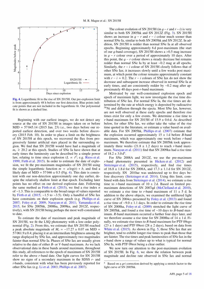
Fig. 4. Logarithmic fit to the rise of SN 2015H. Our pre-explosion limitis from approximately 48 h before our first detection. Blue points indi-cate points that are not included in the logarithmic fit. Our polynomialfit is shown as a dashed line.

Beginning with our earliest images, we do not detect anysource at the site of SN 2015H in images taken on or beforeMJD = 57 045.14 (2015 Jan. 23) i.e., two days before our re-ported earliest detection, and over two weeks before discov-ery (2015 Feb. 10). In order to place a limit on the brightnessof SN 2015H at this epoch, we recovered the flux from pro-gressively fainter artificial stars placed in the surrounding re-gion. We find that SN 2015H would have had a magnitude ofmr >∼ 20.2 at this epoch. Studies of SNe Ia have shown that atearly times the luminosity can be described by a simple powerlaw, relating to time since explosion (L ∝ tn; e.g. Riess et al.1999; Firth et al. 2015). In order to estimate the date of explo-sion, we fit the pre-maximum magnitudes of SN 2015H usingthe simple logarithmic function m = a log(t) + b, and find alikely date of MJD = 57 046 ± 0.5 (Fig. 4). This date is consis-tent with our non-detection approximately one day earlier, de-spite the relatively shallow limit at that epoch. Excluding laterpoints has no effect on our derived explosion date. Followingthe same method as Firth et al. (2015), we find a rise index nof ∼1.3. This is comparable to the broad range of values reportedby Firth et al. (2015; ∼1.5 to ∼3.5). Only a handful of SNe Iaxhave constraints on their explosion epoch (e.g. Phillips et al.2007; Foley et al. 2009; Narayan et al. 2011; Yamanaka et al.2015, for SNe 2005hk, 2008ha, 2009ku, and 2012Z, respec-tively), with SN 2015H being perhaps the most well-constrainedto date.

To estimate the date of maximum and peak magnitude ofSN 2015H, we fit the LSQ photometry with a low-order poly-nomial (Fig. 2). From this, we estimate that SN 2015H reacheda peak absolute magnitude of Mr = −17.27 ± 0.07 on MJD =57 061.9±0.4; placing it at an intermediate brightness among therange displayed by SNe Iax, and approximately two magnitudesfainter than normal SNe Ia. Phases of SNe Iax are usually givenrelative to the date of either B- or V-band maximum. As we lackobservational data in these bands around maximum, throughoutthis study, all references to the epoch of maximum of SN 2015Hrefer to the above r-band date. Our light curves for SN 2015Hshow no signs of a secondary maximum in the SDSS r- andi-bands, consistent with what has been previously reported forother SNe Iax (e.g. Li et al. 2003; Phillips et al. 2007).

The colour evolution of SN 2015H (in g− r and r− i) is verysimilar to both SN 2005hk and SN 2012Z (Fig. 3). SN 2015Hshows an increase in g − r and r − i colour much sooner thannormal SNe Ia, similar to both SN 2005hk and SN 2012Z. In ad-dition, SN 2015H is redder than normal SNe Ia at all observedepochs. Beginning approximately 6 d post-maximum (the startof our g-band coverage), SN 2015H shows a >0.5 mag increasein g − r colour over a period of approximately 10 days. Afterthis point, the g − r colour shows a steady decrease but remainsredder than normal SNe Ia by at least ∼0.2 mag at all epochs.Similarly, the r − i colour of SN 2015H closely follows that ofother SNe Iax; it increases slowly until a few weeks post maxi-mum, at which point the colour remains approximately constantwith r − i ' 0.2. The r − i colours of SNe Iax do not show thedecrease and subsequent increase observed in normal SNe Ia atearly times, and are consistently redder by ∼0.2 mag after ap-proximately 40 days post-r-band maximum.

Motivated by our well-constrained explosion epoch andepoch of maximum light, we now investigate the rise time dis-tribution of SNe Iax. For normal SNe Ia, the rise times are de-termined by the rate at which energy is deposited by radioactive56Ni and diffusion through the ejecta. Most SNe Iax, however,are not well observed at these early epochs and therefore risetimes exist for only a few events. We determine a rise time tor-band maximum for SN 2015H of 15.9 ± 0.6 d. As describedbelow, for other SNe Iax, we either take the value of the risetime quoted in the literature, or estimate a value based on avail-able data. For SN 2005hk, Phillips et al. (2007) estimate thatthe explosion occurred approximately 15 ± 1 d before B-bandmaximum, which was approximately one week before r-bandmaximum. We therefore estimate that SN 2005hk took approx-imately three weeks (21.8 ± 1.2 days) to reach r-band maxi-mum. Narayan et al. (2011) find that SN 2009ku had a rise timeof 18.2 ± 3.0 d6.

For SNe 2008A and 2012Z, we use the pre-maximumr-band photometry presented in Hicken et al. (2012) andStritzinger et al. (2015), respectively, and find rise timesof 16.8 ± 1.8 d for SN 2008A, and 17.3 ± 1.1 d for SN 2012Z,respectively. SN 2010ae was undetected up to five days be-fore discovery (Stritzinger et al. 2014). Using this limit, com-bined with data from Stritzinger et al. (2014), we estimate a risetime to r-band maximum of 10 ± 2 d. Based on limited pre-maximum detections of SN 2007qd (McClelland et al. 2010),we estimate a rise time to r-band maximum of 11 ± 5 d. Inaddition to the above objects, we examined the unfiltered lightcurve of SN 2004cs presented by Foley et al. (2013) and founda rise time of ∼9.0 ± 1.1 days. In order to estimate the rise timeof SN 2008ha, Foley et al. (2009) stretched the light curve ofSN 2005hk, and found a rise time of ∼10 days to B-band max-imum. R-band maximum occurred a further four days later, andwe therefore assume a rise time for SN 2008ha of 14 ± 1 d. Fi-nally, we estimate rise times to R-band maximum for PTF 09ego(23 ± 1 days) and PTF 09eoi (28 ± 2 days), based on data fromWhite et al. (2015). As shown in Fig. 5, those SNe Iax that arebrighter, tend to exhibit longer rise times to peak than those thatare fainter. The rise times and peak luminosities of SNe Iax in ther-band show a range of values up to what is typical for normalSNe Ia, with PTF 09eoi being a clear outlier.

We now turn our attention to the post-maximum evolutionof SN 2015H. In Fig. 6, we show the relation between peakmagnitude and decline rate observed in SNe Iax and normal

6 Based on a gri correction derived by applying a stretch factor to thelight curve of SN 2005hk.

A89, page 5 of 18

A&A 589, A89 (2016)

-20

-19

-18

-17

-16

-15

-14

5 10 15 20 25 30

15H

05hk

09ku

08A

12Z

10ae

04cs

08ha

09ego

09eoi

07qd

02cx

04eo

05cf

11fe

N1def

N3defN5def

SNe Iax r RNormal SNe IaModel

Peak Absolute Magnitude

Rise Time (days)

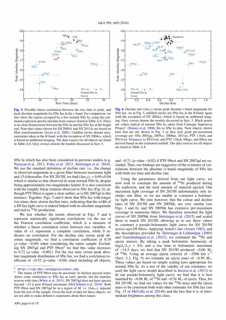
Fig. 5. Possible linear correlation between the rise time to peak, andpeak absolute magnitude for SNe Iax in the r-band. For comparison, wealso show the region occupied by a few normal SNe Ia, using the esti-mated explosion epochs and data from sources listed in Table A.8. Thereis no clear demarcation between the SNe Ia and the SNe Iax at the brightend. Note that values shown for SN 2005cf and SN 2011fe are based onfilter transformations (Jester et al. 2005). Unfilled circles denote mea-surements taken in the R-band, with the exception of SN 2004cs, whichis based on unfiltered imaging. The data sources for all objects are listedin Table A.8. Grey crosses denote the models discussed in Sect. 5.

SNe Ia which has also been considered in previous studies (e.g.Narayan et al. 2011; Foley et al. 2013; Stritzinger et al. 2014).We use the standard definition of decline rate: i.e., the changein observed magnitude in a given filter between maximum lightand 15 d thereafter. For SN 2015H, we find (∆m15)r = 0.69±0.04which is similar to that observed in some normal SNe Ia, despitebeing approximately two magnitudes fainter. It is also consistentwith the roughly linear relation observed in SNe Iax (Fig. 6), al-though PTF 09eoi is again a clear outlier, as is SN 2007qd in thisinstance. Together, Figs. 5 and 6 show that SNe Iax with longerrise times show slower decline rates, indicating that the width ofa SN Iax light curve is indeed linked with its absolute magnitudeand tied to 56Ni production.

We test whether the trends observed in Figs. 5 and 6represent statistically significant correlations via the use ofthe Pearson correlation coefficient, which is a measure ofwhether a linear correlation exists between two variables. Avalue of ±1 represents a complete correlation, while 0 in-dicates no correlation. For the decline rate versus peak ab-solute magnitude, we find a correlation coefficient of 0.39(p-value ∼0.09) when considering the entire sample. Exclud-ing SN 2007qd and PTF 09eoi8 we find this value increasesto 0.72 (p-value ∼0.001). For the rise time versus peak abso-lute magnitude distribution of SNe Iax, we find a correlation co-efficient of −0.52 (p-value ∼0.08) when including all objects,

6 http://csp.obs.carnegiescience.edu8 The nature of PTF 09eoi may be uncertain: its limited spectral seriesshows some similarities to SNe Iax at early epochs, but the matchesworsen with time (White et al. 2015). SN 2007qd does not have spectrabeyond ∼15 d post B-band maximum (McClelland et al. 2010). BothPTF 09eoi and SN 2007qd lie in a region of Mr vs. (∆m15)r separatefrom the rest of the sample. Given the lack of data for these objects, weare not able to make definitive statements about their nature.

-20

-19

-18

-17

-16

-15

-14

0 0.2 0.4 0.6 0.8 1 1.2 1.4

15H

05hk08A 08ae

09ku11ay 12Z

10ae08ha

09J

05cc03gq

02cx

09ego

09eoi

11hyh

04cs

PS15csd

07qd

Normal Ia

N5def

N3def

N1def

SNe Iax r RNormal SNe IaModel

Peak Absolute Magnitude

Decline Rate

Fig. 6. Decline rate (∆m15) versus peak absolute r-band magnitude forSNe Iax. As in Fig. 5, unfilled circles are SNe Iax in the R-band, againwith the exception of SN 2004cs, which is based on unfiltered imag-ing. Grey crosses denote the models discussed in Sect. 5. Black pointsare values typical of normal SNe Ia, taken from Carnegie SupernovaProject7 (Hamuy et al. 2006) fits to SNe Ia data. Note objects shownhere that are not shown in Fig. 5 as they lack good pre-maximumcoverage are: SNe 2003gq, 2005cc, 2008ae, 2011ay, PTF 11hyh, andPS15csd. Distances to PS15csd, and PTF 11hyh, 09ego, and 09eoi arederived based on the estimated redshift. The data sources for all objectsare listed in Table A.8.

and −0.71 (p-value ∼0.02) if PTF 09eoi and SN 2007qd are ex-cluded. Thus, our findings are suggestive of the existence of cor-relations between the absolute (r-band) magnitude of SNe Iaxwith both rise time and decline rate.

Using the parameters derived from our light curve, wenow seek to constrain the amount of 56Ni produced duringthe explosion, and the total amount of material ejected. Ourmaximum light coverage of SN 2015H unfortunately only in-cludes one filter, so we are unable to construct a bolomet-ric light curve. We note however, that the colour and declinerates of SN 2015H and SN 2005hk, are very similar (seeFigs. 3 and 6), and SN 2005hk has extensive pre-maximumcoverage in numerous filters. We therefore stretched the lightcurves of SN 2005hk from Stritzinger et al. (2015) and scaledthem to match SN 2015H, allowing us to use these valuesto construct a pseudo-bolometric light curve for SN 2015Hacross ugriJH filters. Applying Arnett’s law (Arnett 1982), andthe descriptions provided by Stritzinger & Leibundgut (2005)and Ganeshalingam et al. (2012), we estimated the 56Ni andejecta masses. By taking a peak bolometric luminosity oflog(L/L�) = 8.6, and a rise time to bolometric maximumof ∼14.5 days, we find that SN 2015H produced ∼0.06 M�of 56Ni. Using an average ejecta velocity of ∼5500 km s−1

(Sect. 3.3, Fig. 9) we estimate an ejecta mass of ∼0.50 M�.These values are based on simple scaling laws appropriate fornormal SNe Ia. As a test of the validity of our estimates, weused the light curve model described in Inserra et al. (2013) tofit our pseudo-bolometric light curve; we find that it is bestmatched by ∼0.06 M� of 56Ni and ∼0.54 M� of ejecta. Thus, forSN 2015H, we find our values for the 56Ni mass and the ejectamass to be consistent both with other estimates for SNe Iax (seeFig. 15 of McCully et al. 2014b) and the fact that it is of inter-mediate brightness among this class.

A89, page 6 of 18

M. R. Magee et al.: SN 2015H

0

5

10

15

20

25

3000 4000 5000 6000 7000 8000 9000 10000 11000 12000 13000 14000 15000 16000

+3

+6

+10+16

+17

+31

+47

+113

+7

+16

+30

Ca IIFe II

Fe II+Si II?

Fe II+O I?

Co IIFe II Fe II

Flux +

Constant (10-16 erg s-1 cm-2

Å-1)

Rest Wavelength (Å)

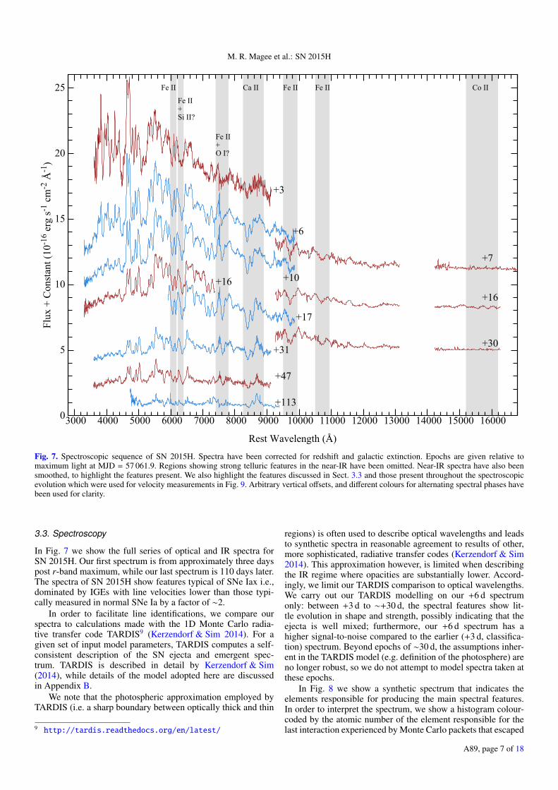
Fig. 7. Spectroscopic sequence of SN 2015H. Spectra have been corrected for redshift and galactic extinction. Epochs are given relative tomaximum light at MJD = 57 061.9. Regions showing strong telluric features in the near-IR have been omitted. Near-IR spectra have also beensmoothed, to highlight the features present. We also highlight the features discussed in Sect. 3.3 and those present throughout the spectroscopicevolution which were used for velocity measurements in Fig. 9. Arbitrary vertical offsets, and different colours for alternating spectral phases havebeen used for clarity.

3.3. Spectroscopy

In Fig. 7 we show the full series of optical and IR spectra forSN 2015H. Our first spectrum is from approximately three dayspost r-band maximum, while our last spectrum is 110 days later.The spectra of SN 2015H show features typical of SNe Iax i.e.,dominated by IGEs with line velocities lower than those typi-cally measured in normal SNe Ia by a factor of ∼2.

In order to facilitate line identifications, we compare ourspectra to calculations made with the 1D Monte Carlo radia-tive transfer code TARDIS9 (Kerzendorf & Sim 2014). For agiven set of input model parameters, TARDIS computes a self-consistent description of the SN ejecta and emergent spec-trum. TARDIS is described in detail by Kerzendorf & Sim(2014), while details of the model adopted here are discussedin Appendix B.

We note that the photospheric approximation employed byTARDIS (i.e. a sharp boundary between optically thick and thin

9 http://tardis.readthedocs.org/en/latest/

regions) is often used to describe optical wavelengths and leadsto synthetic spectra in reasonable agreement to results of other,more sophisticated, radiative transfer codes (Kerzendorf & Sim2014). This approximation however, is limited when describingthe IR regime where opacities are substantially lower. Accord-ingly, we limit our TARDIS comparison to optical wavelengths.We carry out our TARDIS modelling on our +6 d spectrumonly: between +3 d to ∼+30 d, the spectral features show lit-tle evolution in shape and strength, possibly indicating that theejecta is well mixed; furthermore, our +6 d spectrum has ahigher signal-to-noise compared to the earlier (+3 d, classifica-tion) spectrum. Beyond epochs of ∼30 d, the assumptions inher-ent in the TARDIS model (e.g. definition of the photosphere) areno longer robust, so we do not attempt to model spectra taken atthese epochs.

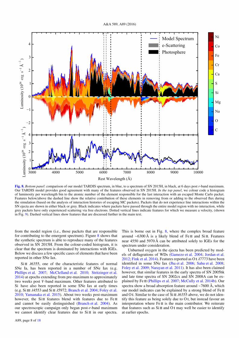
In Fig. 8 we show a synthetic spectrum that indicates theelements responsible for producing the main spectral features.In order to interpret the spectrum, we show a histogram colour-coded by the atomic number of the element responsible for thelast interaction experienced by Monte Carlo packets that escaped

A89, page 7 of 18

A&A 589, A89 (2016)

Fig. 8. Bottom panel: comparison of our model TARDIS spectrum, in blue, to a spectrum of SN 2015H, in black, at 6 days post r-band maximum.Our TARDIS model provides good agreement with many of the features observed in SN 2015H. In the top panel, we colour code a histogramof luminosity per wavelength bin to the atomic number of the element responsible for the last interaction with an escaped Monte Carlo packet.Features below/above the dashed line show the relative contribution of these elements in removing from or adding to the observed flux duringthe simulation (based on the analysis of interaction histories of escaping MC packets). Packets that do not experience line interactions within theSN ejecta are shown in either black or grey. Black indicates where packets have passed through the entire model region with no interaction, whilegrey packets have only experienced scattering via free electrons. Dotted vertical lines indicate features for which we measure a velocity, (shownin Fig. 9). Dashed vertical lines show features that are discussed further in the main text.

from the model region (i.e., those packets that are responsiblefor contributing to the emergent spectrum). Figure 8 shows thatthe synthetic spectrum is able to reproduce many of the featuresobserved in SN 2015H. From the colour-coded histogram, it isclear that the spectrum is dominated by interactions with IGEs.Below we discuss a few specific cases of elements that have beenreported in other SNe Iax.

Si ii λ6355, one of the characteristic features of normalSNe Ia, has been reported in a number of SNe Iax (e.g.Phillips et al. 2007; McClelland et al. 2010; Stritzinger et al.2014) at epochs extending from pre-maximum to approximatelytwo weeks post V-band maximum. Other features attributed toSi have also been reported in some SNe Iax at early times(e.g. Si iii λ4553 and Si ii λ5972; Branch et al. 2004; Foley et al.2010; Yamanaka et al. 2015). About two weeks post-maximumhowever, the Si ii features blend with features due to Fe iiand cannot be easily distinguished (Branch et al. 2004). Asour spectroscopic campaign only began post-r-band maximumwe cannot identify clear features due to Si ii in our spectra.

This is borne out in Fig. 8, where the complex broad featurearound ∼6300 Å is a likely blend of Fe ii and Si ii. Featuresnear 4550 and 5970 Å can be attributed solely to IGEs for thespectrum under consideration.

Unburned oxygen in the ejecta has been predicted by mod-els of deflagrations of WDs (Gamezo et al. 2004; Jordan et al.2012; Fink et al. 2014). Features reported as O i λ7773 have beenidentified in some SNe Iax (Jha et al. 2006; Sahu et al. 2008;Foley et al. 2009; Narayan et al. 2011). It has also been claimedhowever, that similar features in the early spectra of SN 2005hkand late time spectra of SN 2002cx and SN 2008A can be ex-plained by Fe ii (Phillips et al. 2007; McCully et al. 2014b). Ourspectra show a broad absorption feature around ∼7600 Å, whichour model indicates can be explained by a strong blend of Fe iiand O i. Similar to the case of Si ii λ6355 above, we do not iden-tify this feature as being solely due to O i, but instead favour aninterpretation where Fe ii is the main contributor. We reiteratethat features such as Si ii and O i may well be easier to identifyat earlier epochs.

A89, page 8 of 18

M. R. Magee et al.: SN 2015H

Having identified the dominant ions shaping our opticalspectrum, we now wish to identify the dominant species respon-sible for the near-IR flux. While the TARDIS model discussedabove is unsuitable for this purpose, the more sophisticatedsimulations discussed further in Sect. 5 can be used for this pur-pose. Based on comparing our spectra to these models, we findthat as for the optical spectrum, our 1−1.6 µm spectrum takenat +16 d is dominated by IGEs, in particular Fe ii features andweak Co ii (Fig. 7).

As with SNe Ia, the detection of H or He in spectra ofSNe Iax could be key to shedding light on the progenitor chan-nel(s). Indeed, the recent intriguing detection of the progen-itor of the SN Iax 2012Z, has characteristics reminiscent ofthat of some He novae (McCully et al. 2014a). Possible de-tections of He i (λ5876, λ6678, λ7065) have in fact been re-ported for two SNe Iax: SNe 2004cs10 (Foley et al. 2013) and2007J11 (Foley et al. 2009), although whether these two objectsare bona fide members of this class is contentious (White et al.2015).

The atomic energy levels associated with the optical transi-tions of He i are difficult to excite, so the lack of strong He i fea-tures in optical spectra is not surprising, and does not necessar-ily imply that it is not present in the progenitor system (e.g.Hachinger et al. 2012). Currently, we cannot comment furtheron optical features (due to the lack of a sufficiently sophisticatedtreatment of non-thermal excitation/ionization of He in our mod-els), but we note that at the epoch under consideration, featuresdue to IGEs dominate the spectrum.

Strong He i transitions do exist however, at near-IR wave-lengths e.g., the 1s2s 3S – 1s2p 3P transition at 10 830 Å. ManySNe Iax lack observations at these wavelengths; for SN 2015H,not only do we cover this region, but our three near-IR spectrawere taken at epochs comparable to those of SN 2007J for whichthe putative He i feature was reported to be growing strongerwith time (Filippenko et al. 2007b). In SN 2015H, we find abroad feature around ∼10 700 Å, but the inferred velocities aretoo low when compared with other species to plausibly identifythis feature as He i. Based on models described in Sect. 5, wefind good agreement for this feature with Fe ii, and consider thisto be a more plausible identification.

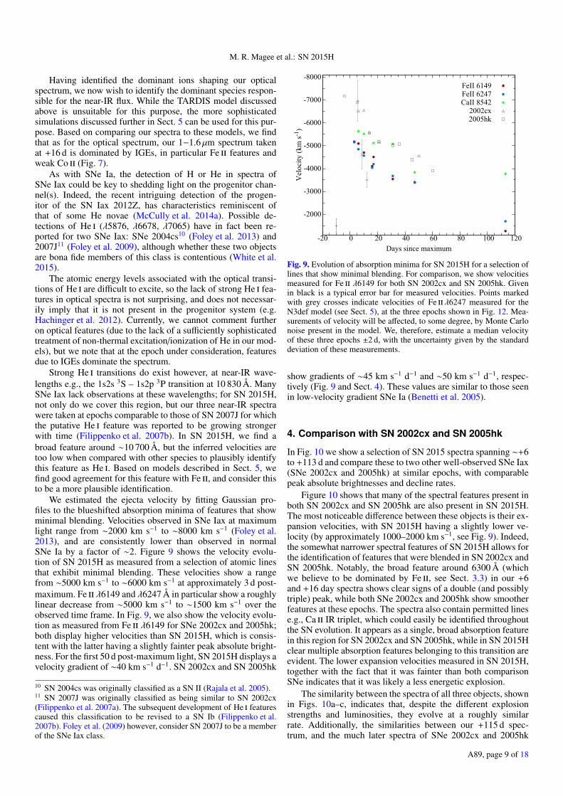
We estimated the ejecta velocity by fitting Gaussian pro-files to the blueshifted absorption minima of features that showminimal blending. Velocities observed in SNe Iax at maximumlight range from ∼2000 km s−1 to ∼8000 km s−1 (Foley et al.2013), and are consistently lower than observed in normalSNe Ia by a factor of ∼2. Figure 9 shows the velocity evolu-tion of SN 2015H as measured from a selection of atomic linesthat exhibit minimal blending. These velocities show a rangefrom ∼5000 km s−1 to ∼6000 km s−1 at approximately 3 d post-maximum. Fe ii λ6149 and λ6247 Å in particular show a roughlylinear decrease from ∼5000 km s−1 to ∼1500 km s−1 over theobserved time frame. In Fig. 9, we also show the velocity evolu-tion as measured from Fe ii λ6149 for SNe 2002cx and 2005hk;both display higher velocities than SN 2015H, which is consis-tent with the latter having a slightly fainter peak absolute bright-ness. For the first 50 d post-maximum light, SN 2015H displays avelocity gradient of ∼40 km s−1 d−1. SN 2002cx and SN 2005hk

10 SN 2004cs was originally classified as a SN II (Rajala et al. 2005).11 SN 2007J was originally classified as being similar to SN 2002cx(Filippenko et al. 2007a). The subsequent development of He i featurescaused this classification to be revised to a SN Ib (Filippenko et al.2007b). Foley et al. (2009) however, consider SN 2007J to be a memberof the SNe Iax class.

-8000

-7000

-6000

-5000

-4000

-3000

-2000

-20 0 20 40 60 80 100 120

Velocity (km

s-1 )

Days since maximum

FeII 6149FeII 6247CaII 85422002cx2005hk

Fig. 9. Evolution of absorption minima for SN 2015H for a selection oflines that show minimal blending. For comparison, we show velocitiesmeasured for Fe ii λ6149 for both SN 2002cx and SN 2005hk. Givenin black is a typical error bar for measured velocities. Points markedwith grey crosses indicate velocities of Fe ii λ6247 measured for theN3def model (see Sect. 5), at the three epochs shown in Fig. 12. Mea-surements of velocity will be affected, to some degree, by Monte Carlonoise present in the model. We, therefore, estimate a median velocityof these three epochs ±2 d, with the uncertainty given by the standarddeviation of these measurements.

show gradients of ∼45 km s−1 d−1 and ∼50 km s−1 d−1, respec-tively (Fig. 9 and Sect. 4). These values are similar to those seenin low-velocity gradient SNe Ia (Benetti et al. 2005).

4. Comparison with SN 2002cx and SN 2005hk

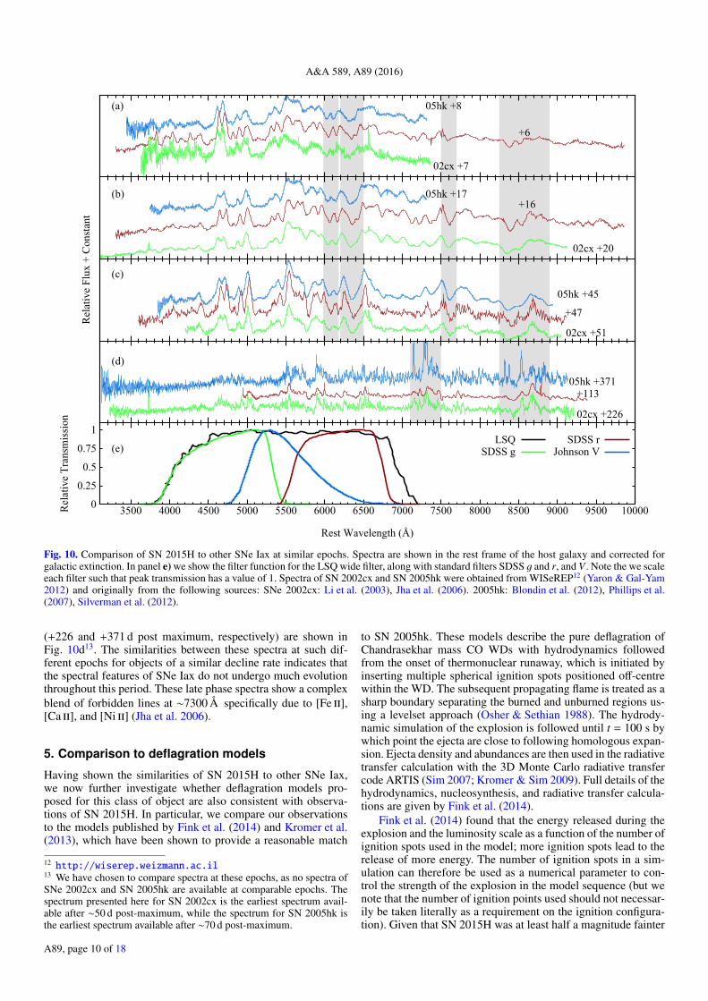
In Fig. 10 we show a selection of SN 2015 spectra spanning ∼+6to +113 d and compare these to two other well-observed SNe Iax(SNe 2002cx and 2005hk) at similar epochs, with comparablepeak absolute brightnesses and decline rates.

Figure 10 shows that many of the spectral features present inboth SN 2002cx and SN 2005hk are also present in SN 2015H.The most noticeable difference between these objects is their ex-pansion velocities, with SN 2015H having a slightly lower ve-locity (by approximately 1000–2000 km s−1, see Fig. 9). Indeed,the somewhat narrower spectral features of SN 2015H allows forthe identification of features that were blended in SN 2002cx andSN 2005hk. Notably, the broad feature around 6300 Å (whichwe believe to be dominated by Fe ii, see Sect. 3.3) in our +6and +16 day spectra shows clear signs of a double (and possiblytriple) peak, while both SNe 2002cx and 2005hk show smootherfeatures at these epochs. The spectra also contain permitted linese.g., Ca ii IR triplet, which could easily be identified throughoutthe SN evolution. It appears as a single, broad absorption featurein this region for SN 2002cx and SN 2005hk, while in SN 2015Hclear multiple absorption features belonging to this transition areevident. The lower expansion velocities measured in SN 2015H,together with the fact that it was fainter than both comparisonSNe indicates that it was likely a less energetic explosion.

The similarity between the spectra of all three objects, shownin Figs. 10a–c, indicates that, despite the different explosionstrengths and luminosities, they evolve at a roughly similarrate. Additionally, the similarities between our +115 d spec-trum, and the much later spectra of SNe 2002cx and 2005hk

A89, page 9 of 18

A&A 589, A89 (2016)

05hk +8

+6

02cx +7

(a)

05hk +17+16

02cx +20

(b)

05hk +45

+47

02cx +51

(c)

Relative Flux +

Constant

05hk +371

02cx +226

+113

(d)

0

0.25

0.5

0.75

1

3500 4000 4500 5000 5500 6000 6500 7000 7500 8000 8500 9000 9500 10000

(e)

Relative Transmission

Rest Wavelength (Å)

LSQSDSS g

SDSS rJohnson V

Fig. 10. Comparison of SN 2015H to other SNe Iax at similar epochs. Spectra are shown in the rest frame of the host galaxy and corrected forgalactic extinction. In panel e) we show the filter function for the LSQ wide filter, along with standard filters SDSS g and r, and V . Note the we scaleeach filter such that peak transmission has a value of 1. Spectra of SN 2002cx and SN 2005hk were obtained from WISeREP12 (Yaron & Gal-Yam2012) and originally from the following sources: SNe 2002cx: Li et al. (2003), Jha et al. (2006). 2005hk: Blondin et al. (2012), Phillips et al.(2007), Silverman et al. (2012).

(+226 and +371 d post maximum, respectively) are shown inFig. 10d13. The similarities between these spectra at such dif-ferent epochs for objects of a similar decline rate indicates thatthe spectral features of SNe Iax do not undergo much evolutionthroughout this period. These late phase spectra show a complexblend of forbidden lines at ∼7300 Å specifically due to [Fe ii],[Ca ii], and [Ni ii] (Jha et al. 2006).

5. Comparison to deflagration models

Having shown the similarities of SN 2015H to other SNe Iax,we now further investigate whether deflagration models pro-posed for this class of object are also consistent with observa-tions of SN 2015H. In particular, we compare our observationsto the models published by Fink et al. (2014) and Kromer et al.(2013), which have been shown to provide a reasonable match

12 http://wiserep.weizmann.ac.il13 We have chosen to compare spectra at these epochs, as no spectra ofSNe 2002cx and SN 2005hk are available at comparable epochs. Thespectrum presented here for SN 2002cx is the earliest spectrum avail-able after ∼50 d post-maximum, while the spectrum for SN 2005hk isthe earliest spectrum available after ∼70 d post-maximum.

to SN 2005hk. These models describe the pure deflagration ofChandrasekhar mass CO WDs with hydrodynamics followedfrom the onset of thermonuclear runaway, which is initiated byinserting multiple spherical ignition spots positioned off-centrewithin the WD. The subsequent propagating flame is treated as asharp boundary separating the burned and unburned regions us-ing a levelset approach (Osher & Sethian 1988). The hydrody-namic simulation of the explosion is followed until t = 100 s bywhich point the ejecta are close to following homologous expan-sion. Ejecta density and abundances are then used in the radiativetransfer calculation with the 3D Monte Carlo radiative transfercode ARTIS (Sim 2007; Kromer & Sim 2009). Full details of thehydrodynamics, nucleosynthesis, and radiative transfer calcula-tions are given by Fink et al. (2014).

Fink et al. (2014) found that the energy released during theexplosion and the luminosity scale as a function of the number ofignition spots used in the model; more ignition spots lead to therelease of more energy. The number of ignition spots in a sim-ulation can therefore be used as a numerical parameter to con-trol the strength of the explosion in the model sequence (but wenote that the number of ignition points used should not necessar-ily be taken literally as a requirement on the ignition configura-tion). Given that SN 2015H was at least half a magnitude fainter

A89, page 10 of 18

M. R. Magee et al.: SN 2015H

-19

-18

-17

-16

-15

-14� � � � � �

g

Absolute Magnitude

� � � � � �

V N5defN3defN1def

-18

-17

-16

-15

-14 5 15 25 35 45

r

Days since explosion5 15 25 35 45

i

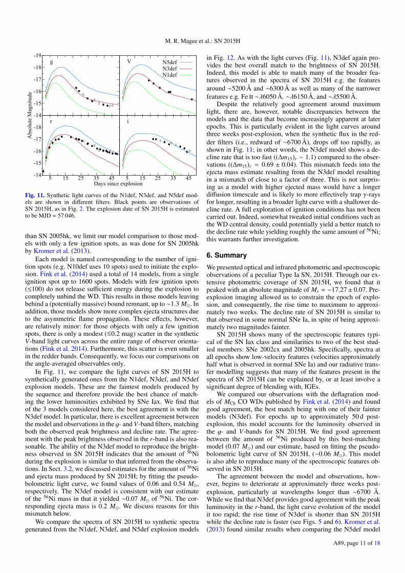
Fig. 11. Synthetic light curves of the N1def, N3def, and N5def mod-els are shown in different filters. Black points are observations ofSN 2015H, as in Fig. 2. The explosion date of SN 2015H is estimatedto be MJD = 57 046.

than SN 2005hk, we limit our model comparison to those mod-els with only a few ignition spots, as was done for SN 2005hkby Kromer et al. (2013).

Each model is named corresponding to the number of igni-tion spots (e.g. N10def uses 10 spots) used to initiate the explo-sion. Fink et al. (2014) used a total of 14 models, from a singleignition spot up to 1600 spots. Models with few ignition spots(≤100) do not release sufficient energy during the explosion tocompletely unbind the WD. This results in those models leavingbehind a (potentially massive) bound remnant, up to ∼1.3 M�. Inaddition, those models show more complex ejecta structures dueto the asymmetric flame propagation. These effects, however,are relatively minor: for those objects with only a few ignitionspots, there is only a modest (<∼0.2 mag) scatter in the syntheticV-band light curves across the entire range of observer orienta-tions (Fink et al. 2014). Furthermore, this scatter is even smallerin the redder bands. Consequently, we focus our comparisons onthe angle-averaged observables only.

In Fig. 11, we compare the light curves of SN 2015H tosynthetically generated ones from the N1def, N3def, and N5defexplosion models. These are the faintest models produced bythe sequence and therefore provide the best chance of match-ing the lower luminosities exhibited by SNe Iax. We find thatof the 3 models considered here, the best agreement is with theN3def model. In particular, there is excellent agreement betweenthe model and observations in the g- and V-band filters, matchingboth the observed peak brightness and decline rate. The agree-ment with the peak brightness observed in the r-band is also rea-sonable. The ability of the N3def model to reproduce the bright-ness observed in SN 2015H indicates that the amount of 56Niduring the explosion is similar to that inferred from the observa-tions. In Sect. 3.2, we discussed estimates for the amount of 56Niand ejecta mass produced by SN 2015H; by fitting the pseudo-bolometric light curve, we found values of 0.06 and 0.54 M�,respectively. The N3def model is consistent with our estimateof the 56Ni mass in that it yielded ∼0.07 M� of 56Ni. The cor-responding ejecta mass is 0.2 M�. We discuss reasons for thismismatch below.

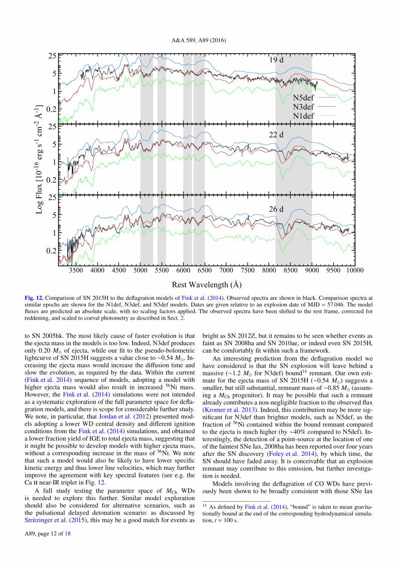
We compare the spectra of SN 2015H to synthetic spectragenerated from the N1def, N3def, and N5def explosion models

in Fig. 12. As with the light curves (Fig. 11), N3def again pro-vides the best overall match to the brightness of SN 2015H.Indeed, this model is able to match many of the broader fea-tures observed in the spectra of SN 2015H e.g. the featuresaround ∼5200 Å and ∼6300 Å as well as many of the narrowerfeatures e.g. Fe ii ∼λ6050 Å. ∼λ6150 Å, and ∼λ5500 Å.

Despite the relatively good agreement around maximumlight, there are, however, notable discrepancies between themodels and the data that become increasingly apparent at laterepochs. This is particularly evident in the light curves aroundthree weeks post-explosion, when the synthetic flux in the red-der filters (i.e., redward of ∼6700 Å), drops off too rapidly, asshown in Fig. 11; in other words, the N3def model shows a de-cline rate that is too fast ((∆m15)r ∼ 1.1) compared to the obser-vations ((∆m15)r = 0.69 ± 0.04). This mismatch feeds into theejecta mass estimate resulting from the N3def model resultingin a mismatch of close to a factor of three. This is not surpris-ing as a model with higher ejected mass would have a longerdiffusion timescale and is likely to more effectively trap γ-raysfor longer, resulting in a broader light curve with a shallower de-cline rate. A full exploration of ignition conditions has not beencarried out. Indeed, somewhat tweaked initial conditions such asthe WD central density, could potentially yield a better match tothe decline rate while yielding roughly the same amount of 56Ni;this warrants further investigation.

6. Summary

We presented optical and infrared photometric and spectroscopicobservations of a peculiar Type Ia SN, 2015H. Through our ex-tensive photometric coverage of SN 2015H, we found that itpeaked with an absolute magnitude of Mr = −17.27 ± 0.07. Pre-explosion imaging allowed us to constrain the epoch of explo-sion, and consequently, the rise time to maximum to approxi-mately two weeks. The decline rate of SN 2015H is similar tothat observed in some normal SNe Ia, in spite of being approxi-mately two magnitudes fainter.

SN 2015H shows many of the spectroscopic features typi-cal of the SN Iax class and similarities to two of the best stud-ied members: SNe 2002cx and 2005hk. Specifically, spectra atall epochs show low-velocity features (velocities approximatelyhalf what is observed in normal SNe Ia) and our radiative trans-fer modelling suggests that many of the features present in thespectra of SN 2015H can be explained by, or at least involve asignificant degree of blending with, IGEs.

We compared our observations with the deflagration mod-els of MCh CO WDs published by Fink et al. (2014) and foundgood agreement, the best match being with one of their faintermodels (N3def). For epochs up to approximately 50 d post-explosion, this model accounts for the luminosity observed inthe g- and V-bands for SN 2015H. We find good agreementbetween the amount of 56Ni produced by this best-matchingmodel (0.07 M�) and our estimate, based on fitting the pseudo-bolometric light curve of SN 2015H, (∼0.06 M�). This modelis also able to reproduce many of the spectroscopic features ob-served in SN 2015H.

The agreement between the model and observations, how-ever, begins to deteriorate at approximately three weeks post-explosion, particularly at wavelengths longer than ∼6700 Å.While we find that N3def provides good agreement with the peakluminosity in the r-band, the light curve evolution of the modelit too rapid; the rise time of N3def is shorter than SN 2015Hwhile the decline rate is faster (see Figs. 5 and 6). Kromer et al.(2013) found similar results when comparing the N5def model

A89, page 11 of 18

A&A 589, A89 (2016)

0.2

1

5

25

19 d

N1defN3defN5def

0.2

1

5

25

22 d

Log

Flux [10-16

erg s-1 cm-2

Å-1]

0.2

1

5

25

3500 4000 4500 5000 5500 6000 6500 7000 7500 8000 8500 9000 9500 10000

26 d

Rest Wavelength (Å)

Fig. 12. Comparison of SN 2015H to the deflagration models of Fink et al. (2014). Observed spectra are shown in black. Comparison spectra atsimilar epochs are shown for the N1def, N3def, and N5def models. Dates are given relative to an explosion date of MJD = 57 046. The modelfluxes are predicted an absolute scale, with no scaling factors applied. The observed spectra have been shifted to the rest frame, corrected forreddening, and scaled to coeval photometry as described in Sect. 2.

to SN 2005hk. The most likely cause of faster evolution is thatthe ejecta mass in the models is too low. Indeed, N3def producesonly 0.20 M� of ejecta, while our fit to the pseudo-bolometriclightcurve of SN 2015H suggests a value close to ∼0.54 M�. In-creasing the ejecta mass would increase the diffusion time andslow the evolution, as required by the data. Within the current(Fink et al. 2014) sequence of models, adopting a model withhigher ejecta mass would also result in increased 56Ni mass.However, the Fink et al. (2014) simulations were not intendedas a systematic exploration of the full parameter space for defla-gration models, and there is scope for considerable further study.We note, in particular, that Jordan et al. (2012) presented mod-els adopting a lower WD central density and different ignitionconditions from the Fink et al. (2014) simulations, and obtaineda lower fraction yield of IGE to total ejecta mass, suggesting thatit might be possible to develop models with higher ejecta mass,without a corresponding increase in the mass of 56Ni. We notethat such a model would also be likely to have lower specifickinetic energy and thus lower line velocities, which may furtherimprove the agreement with key spectral features (see e.g. theCa ii near-IR triplet in Fig. 12.

A full study testing the parameter space of MCh WDsis needed to explore this further. Similar model explorationshould also be considered for alternative scenarios, such asthe pulsational delayed detonation scenario: as discussed byStritzinger et al. (2015), this may be a good match for events as

bright as SN 2012Z, but it remains to be seen whether events asfaint as SN 2008ha and SN 2010ae, or indeed even SN 2015H,can be comfortably fit within such a framework.

An interesting prediction from the deflagration model wehave considered is that the SN explosion will leave behind amassive (∼1.2 M� for N3def) bound14 remnant. Our own esti-mate for the ejecta mass of SN 2015H (∼0.54 M�) suggests asmaller, but still substantial, remnant mass of ∼0.85 M� (assum-ing a MCh progenitor). It may be possible that such a remnantalready contributes a non-negligible fraction to the observed flux(Kromer et al. 2013). Indeed, this contribution may be more sig-nificant for N3def than brighter models, such as N5def, as thefraction of 56Ni contained within the bound remnant comparedto the ejecta is much higher (by ∼40% compared to N5def). In-terestingly, the detection of a point-source at the location of oneof the faintest SNe Iax, 2008ha has been reported over four yearsafter the SN discovery (Foley et al. 2014), by which time, theSN should have faded away. It is conceivable that an explosionremnant may contribute to this emission, but further investiga-tion is needed.

Models involving the deflagration of CO WDs have previ-ously been shown to be broadly consistent with those SNe Iax

14 As defined by Fink et al. (2014), “bound” is taken to mean gravita-tionally bound at the end of the corresponding hydrodynamical simula-tion, t = 100 s.

A89, page 12 of 18

M. R. Magee et al.: SN 2015H

that are bright (e.g. SN2005hk, Kromer et al. 2013). In thisstudy, we have shown that models of weaker deflagrations inMCh CO WDs producing ∼0.07 M� of 56Ni are able to repro-duce the features observed in fainter events such as SN2015H.Combined with the hybrid CONe WD deflagration model pro-posed for the very faintest members of the class (e.g. SN2008haKromer et al. 2015), this suggests that deflagrations of WDs areable to account for SNe Iax across the entire brightness rangeof SNe Iax. Whether such deflagrations are the sole or domi-nant channel giving rise to SNe Iax requires further investiga-tion, but we conclude that the models discussed here do showpromise, and merit continued investigation and refinement. Wealso stress the need for further observations of this class of su-pernova, including objects that are discovered post-peak, such asSN 2015H.

Acknowledgements. We are grateful to C. White for providing the photomet-ric data on PTF 09eo, 09eoi, 09eiy, and 11hyh in digital form, and U. Nöbauerfor providing TARDIS analysis tools. RK and SAS acknowledge support fromSTFC via ST/L000709/1. This work makes use of observations from the LCOGTnetwork. Based on observations collected at the European Organisation for As-tronomical Research in the Southern Hemisphere, Chile as part of PESSTO, (thePublic ESO Spectroscopic Survey for Transient Objects Survey) ESO programID 188.D-3003. IRS was supported by the Australian Research Council Lau-reate Grant FL0992131. The authors gratefully acknowledge the Gauss Cen-tre for Supercomputing (GCS) for providing computing time through the Johnvon Neumann Institute for Computing (NIC) on the GCS share of the super-computer JUQUEEN at Jülich Supercomputing Centre (JSC). G.C.S. is the al-liance of the three national supercomputing centres HLRS (Universität Stuttgart),JSC (Forschungszentrum Jülich), and LRZ (Bayerische Akademie der Wis-senschaften), funded by the German Federal Ministry of Education and Research(BMBF) and the German State Ministries for Research of Baden-Württemberg(MWK), Bayern (StMWFK) and Nordrhein-Westfalen (MIWF). Support for LGis provided by the Ministry of Economy, Development, and Tourism’s Mil-lennium Science Initiative through grant IC120009, awarded to The Millen-nium Institute of Astrophysics, MAS. L.G. acknowledges support by CONI-CYT through FONDECYT grant 3140566. K.M. acknowledges support from theSTFC through an Ernest Rutherford Fellowship. R.P. acknowledges support bythe European Research Council under ERC-StG grant EXAGAL-308037. S.J.S.acknowledges funding from the European Research Council under the EuropeanUnion’s Seventh Framework Programme (FP7/2007-2013)/ERC Grant agree-ment no. [291222] and STFC grants ST/I001123/1 and ST/L000709/1. W.H. ac-knowledges support by TRR 33 “The Dark Universe” of the German ResearchFoundation (DFG) and the Excellence Cluster EXC153 “Origin and Structure ofthe Universe”. H.C. acknowledges support from the European Union FP7 pro-gramme through ERC grant number 320360. This research has made use of theNASA/IPAC Extragalactic Database (NED) which is operated by the Jet Propul-sion Laboratory, California Institute of Technology, under contract with the Na-tional Aeronautics and Space Administration.

ReferencesArnett, W. D. 1982, ApJ, 253, 785Baltay, C., Rabinowitz, D., Hadjiyska, E., et al. 2013, PASP, 125, 683Benetti, S., Cappellaro, E., Mazzali, P. A., et al. 2005, ApJ, 623, 1011Blondin, S., Matheson, T., Kirshner, R. P., et al. 2012, AJ, 143, 126Branch, D., Fisher, A., & Nugent, P. 1993, AJ, 106, 2383Branch, D., Baron, E., Thomas, R. C., et al. 2004, PASP, 116, 903Brown, T. M., Baliber, N., Bianco, F. B., et al. 2013, PASP, 125, 1031Filippenko, A. V., Richmond, M. W., Matheson, T., et al. 1992, ApJ, 384, L15Filippenko, A. V., Foley, R. J., Silverman, J. M., et al. 2007a, Central Bureau

Electronic Telegrams, 817, 1Filippenko, A. V., Foley, R. J., Silverman, J. M., et al. 2007b, Central Bureau

Electronic Telegrams, 926, 1

Fink, M., Kromer, M., Seitenzahl, I. R., et al. 2014, MNRAS, 438, 1762Firth, R. E., Sullivan, M., Gal-Yam, A., et al. 2015, MNRAS, 446, 3895Fitzpatrick, E. L. 1999, PASP, 111, 63Foley, R. J., Chornock, R., Filippenko, A. V., et al. 2009, AJ, 138, 376Foley, R. J., McCully, C., Jha, S. W., et al. 2014, ApJ, 792, 29Foley, R. J., Brown, P. J., Rest, A., et al. 2010, ApJ, 708, L61Foley, R. J., Challis, P. J., Chornock, R., et al. 2013, ApJ, 767, 57Gamezo, V. N., Khokhlov, A. M., & Oran, E. S. 2004, Phys. Rev. Lett., 92,

211102Ganeshalingam, M., Li, W., Filippenko, A. V., et al. 2012, ApJ, 751, 142Hachinger, S., Mazzali, P. A., Taubenberger, S., et al. 2012, MNRAS, 422, 70Hamuy, M., Folatelli, G., Morrell, N. I., et al. 2006, PASP, 118, 2Hicken, M., Challis, P., Kirshner, R. P., et al. 2012, ApJS, 200, 12Hillebrandt, W., & Niemeyer, J. C. 2000, ARA&A, 38, 191Hillebrandt, W., Kromer, M., Röpke, F. K., & Ruiter, A. J. 2013, Frontiers of

Physics, 8, 116Inserra, C., Smartt, S. J., Jerkstrand, A., et al. 2013, ApJ, 770, 128Jester, S., Schneider, D. P., Richards, G. T., et al. 2005, AJ, 130, 873Jha, S., Branch, D., Chornock, R., et al. 2006, AJ, 132, 189Jordan, IV, G. C., Perets, H. B., Fisher, R. T., & van Rossum, D. R. 2012, ApJ,

761, L23Kerzendorf, W. E., & Sim, S. A. 2014, MNRAS, 440, 387Kromer, M., & Sim, S. A. 2009, MNRAS, 398, 1809Kromer, M., Fink, M., Stanishev, V., et al. 2013, MNRAS, 429, 2287Kromer, M., Ohlmann, S. T., Pakmor, R., et al. 2015, MNRAS, 450, 3045Li, W. D., Qiu, Y. L., Qiao, Q. Y., et al. 1999, AJ, 117, 2709Li, W., Filippenko, A. V., Chornock, R., et al. 2003, PASP, 115, 453Lira, P. 1996, Master’s thesis, Univ. ChileLong, M., Jordan, IV, G. C., van Rossum, D. R., et al. 2014, ApJ, 789, 103Lyman, J. D., James, P. A., Perets, H. B., et al. 2013, MNRAS, 434, 527McClelland, C. M., Garnavich, P. M., Galbany, L., et al. 2010, ApJ, 720, 704McCully, C., Jha, S. W., Foley, R. J., et al. 2014a, Nature, 512, 54McCully, C., Jha, S. W., Foley, R. J., et al. 2014b, ApJ, 786, 134Moriya, T., Tominaga, N., Tanaka, M., et al. 2010, ApJ, 719, 1445Munari, U., & Zwitter, T. 1997, A&A, 318, 269Narayan, G., Foley, R. J., Berger, E., et al. 2011, ApJ, 731, L11Nugent, P. E., Sullivan, M., Cenko, S. B., et al. 2011, Nature, 480, 344Osher, S., & Sethian, J. A. 1988, J. Comput. Phys., 79, 12Parker, S. 2015, Central Bureau Electronic Telegrams, 4093, 2Pastorello, A., Mazzali, P. A., Pignata, G., et al. 2007a, MNRAS, 377, 1531Pastorello, A., Taubenberger, S., Elias-Rosa, N., et al. 2007b, MNRAS, 376,

1301Perlmutter, S., Aldering, G., Goldhaber, G., et al. 1999, ApJ, 517, 565Phillips, M. M., Li, W., Frieman, J. A., et al. 2007, PASP, 119, 360Poznanski, D., Prochaska, J. X., & Bloom, J. S. 2012, MNRAS, 426, 1465Rajala, A. M., Fox, D. B., Gal-Yam, A., et al. 2005, PASP, 117, 132Richmond, M. W., & Smith, H. A. 2012, J. Am. Assoc. Variable Star Observers

(JAAVSO), 40, 872Richmond, M. W., Treffers, R. R., Filippenko, A. V., et al. 1994, AJ, 107, 1022Riess, A. G., Filippenko, A. V., Challis, P., et al. 1998, AJ, 116, 1009Riess, A. G., Filippenko, A. V., Li, W., et al. 1999, AJ, 118, 2675Sahu, D. K., Tanaka, M., Anupama, G. C., et al. 2008, ApJ, 680, 580Schlafly, E. F., & Finkbeiner, D. P. 2011, ApJ, 737, 103Silverman, J. M., Foley, R. J., Filippenko, A. V., et al. 2012, MNRAS, 425, 1789Sim, S. A. 2007, MNRAS, 375, 154Smartt, S. J., Valenti, S., Fraser, M., et al. 2015, A&A, 579, A40Springob, C. M., Masters, K. L., Haynes, M. P., Giovanelli, R., & Marinoni, C.

2009, ApJS, 182, 474Stritzinger, M., & Leibundgut, B. 2005, A&A, 431, 423Stritzinger, M. D., Hsiao, E., Valenti, S., et al. 2014, A&A, 561, A146Stritzinger, M. D., Valenti, S., Hoeflich, P., et al. 2015, A&A, 573, A2Tully, R. B., & Fisher, J. R. 1977, A&A, 54, 661Valenti, S., Pastorello, A., Cappellaro, E., et al. 2009, Nature, 459, 674Wang, B., Meng, X., Liu, D.-D., Liu, Z.-W., & Han, Z. 2014, ApJ, 794, L28White, C. J., Kasliwal, M. M., Nugent, P. E., et al. 2015, ApJ, 799, 52Yamanaka, M., Maeda, K., Kawabata, K. S., et al. 2015, ApJ, 806, 191Yaron, O., & Gal-Yam, A. 2012, PASP, 124, 668Zelaya-Garcia, P., Baumont, S., Mitra, A., et al. 2015, ATel, 7053, 1

A89, page 13 of 18

A&A 589, A89 (2016)

Appendix A: Additional tables

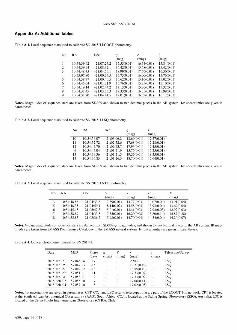
Table A.1. Local sequence stars used to calibrate SN 2015H LCOGT photometry.

No. RA Dec g r i(mag) (mag) (mag)

1 10:54:39.42 –21:07:23.2 17.53(0.01) 16.34(0.01) 15.84(0.01)2 10:54:59.94 –21:08:32.1 16.42(0.01) 15.68(0.01) 15.42(0.01)3 10:54:48.35 –21:04:59.1 18.99(0.01) 17.56(0.01) 16.50(0.01)4 10:55:07.80 –21:00:34.5 16.75(0.01) 16.00(0.01) 15.76(0.01)5 10:54:58.77 –21:00:40.5 15.62(0.01) 15.16(0.01) 15.02(0.01)6 10:54:45.04 –21:01:21.9 15.76(0.01) 15.25(0.01) 15.10(0.01)7 10:54:19.14 –21:02:44.2 17.15(0.01) 15.86(0.01) 15.32(0.01)8 10:54:31.45 –21:03:53.3 17.33(0.01) 16.35(0.01) 15.99(0.01)9 10:54:31.70 –21:04:44.5 17.01(0.01) 16.39(0.01) 16.12(0.01)

Notes. Magnitudes of sequence stars are taken from SDSS9 and shown to two decimal places in the AB system. 1σ uncertainties are given inparentheses.

Table A.2. Local sequence stars used to calibrate SN 2015H LSQ photometry.

No. RA Dec g r(mag) (mag)

10 10:54:54.07 –21:03:06.2 18.60(0.01) 17.27(0.01)11 10:54:52.72 –21:02:52.6 17.68(0.01) 17.28(0.01)12 10:54:47.70 –21:02:43.7 17.93(0.01) 17.45(0.01)

6 10:54:45.04 –21:01:21.9 15.76(0.01) 15.25(0.01)13 10:54:39.36 –21:01:21.5 19.56(0.01) 18.35(0.01)14 10:54:36.85 –21:01:26.5 18.70(0.01) 17.64(0.01)

Notes. Magnitudes of sequence stars are taken from SDSS9 and shown to two decimal places in the AB system. 1σ uncertainties are given inparentheses.

Table A.3. Local sequence stars used to calibrate SN 2015H NTT photometry.

No. RA Dec V J H K(mag) (mag) (mag) (mag)

3 10:54:48.88 –21:04:33.8 17.89(0.01) 14.77(0.03) 14.07(0.04) 13.91(0.05)15 10:54:48.35 –21:04:59.1 18.14(0.02) 14.58(0.04) 13.93(0.04) 13.69(0.04)16 10:54:45.45 –21:05:47.3 15.01(0.01) 13.41(0.03) 12.92(0.03) 12.92(0.03)17 10:54:38.89 –21:04:33.8 17.35(0.01) 16.20(0.08) 15.80(0.14) 15.87(0.28)18 10:54:35.85 –21:03:36.2 15.98(0.01) 14.70(0.04) 14.34(0.04) 14.20(0.07)

Notes. V-band magnitudes of sequence stars are derived from SDSS9 gr magnitudes, and shown to two decimal places in the AB system. IR mag-nitudes are taken from 2MASS Point Source Catalogue in the 2MASS natural system. 1σ uncertainties are given in parentheses.

Table A.4. Optical photometric journal for SN 2015H.

Date MJD Phase g V r i Telescope/Survey(days) (mag) (mag) (mag) (mag)

2015 Jan. 23 57 045.14 −17 ... ... >∼20.2 ... LSQ2015 Jan. 25 57 047.13 −15 ... ... 19.71(0.19) ... LSQ2015 Jan. 27 57 049.12 −13 ... ... 18.55(0.10) ... LSQ2015 Jan. 29 57 051.11 −11 ... ... 17.73(0.07) ... LSQ2015 Jan. 31 57 053.11 −9 ... ... 17.33(0.09) ... LSQ2015 Feb. 02 57 055.10 −7 ... ... 17.08(0.11) ... LSQ2015 Feb. 04 57 057.10 −5 ... ... 17.02(0.05) ... LSQ

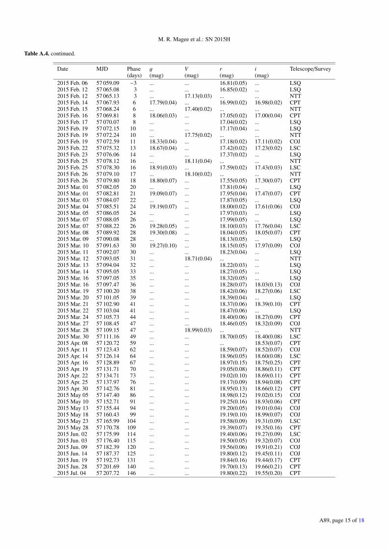
Notes. 1σ uncertainties are given in parentheses. CPT, COJ, and LSC refer to telescopes that are part of the LCOGT 1-m network. CPT is locatedat the South African Astronomical Observatory (SAAO), South Africa; COJ is located at the Siding Spring Observatory (SSO), Australia; LSC islocated at the Cerro Tololo Inter-American Observatory (CTIO), Chile.

A89, page 14 of 18

M. R. Magee et al.: SN 2015H

Table A.4. continued.

Date MJD Phase g V r i Telescope/Survey(days) (mag) (mag) (mag) (mag)

2015 Feb. 06 57 059.09 −3 ... ... 16.81(0.05) ... LSQ2015 Feb. 12 57 065.08 3 ... ... 16.85(0.02) ... LSQ2015 Feb. 12 57 065.13 3 ... 17.13(0.03) ... ... NTT2015 Feb. 14 57 067.93 6 17.79(0.04) ... 16.99(0.02) 16.98(0.02) CPT2015 Feb. 15 57 068.24 6 ... 17.40(0.02) ... ... NTT2015 Feb. 16 57 069.81 8 18.06(0.03) ... 17.05(0.02) 17.00(0.04) CPT2015 Feb. 17 57 070.07 8 ... ... 17.04(0.02) ... LSQ2015 Feb. 19 57 072.15 10 ... ... 17.17(0.04) ... LSQ2015 Feb. 19 57 072.24 10 ... 17.75(0.02) ... ... NTT2015 Feb. 19 57 072.59 11 18.33(0.04) ... 17.18(0.02) 17.11(0.02) COJ2015 Feb. 22 57 075.32 13 18.67(0.04) ... 17.42(0.02) 17.23(0.02) LSC2015 Feb. 23 57 076.06 14 ... ... 17.37(0.02) ... LSQ2015 Feb. 25 57 078.12 16 ... 18.11(0.04) ... ... NTT2015 Feb. 25 57 078.30 16 18.91(0.03) ... 17.59(0.02) 17.43(0.03) LSC2015 Feb. 26 57 079.10 17 ... 18.10(0.02) ... ... NTT2015 Feb. 26 57 079.80 18 18.80(0.07) ... 17.55(0.05) 17.30(0.07) CPT2015 Mar. 01 57 082.05 20 ... ... 17.81(0.04) ... LSQ2015 Mar. 01 57 082.81 21 19.09(0.07) ... 17.95(0.04) 17.47(0.07) CPT2015 Mar. 03 57 084.07 22 ... ... 17.87(0.05) ... LSQ2015 Mar. 04 57 085.51 24 19.19(0.07) ... 18.00(0.02) 17.61(0.06) COJ2015 Mar. 05 57 086.05 24 ... ... 17.97(0.03) ... LSQ2015 Mar. 07 57 088.05 26 ... ... 17.99(0.05) ... LSQ2015 Mar. 07 57 088.22 26 19.28(0.05) ... 18.10(0.03) 17.76(0.04) LSC2015 Mar. 08 57 089.92 28 19.30(0.08) ... 18.04(0.05) 18.05(0.07) CPT2015 Mar. 09 57 090.08 28 ... ... 18.13(0.05) ... LSQ2015 Mar. 10 57 091.63 30 19.27(0.10) ... 18.15(0.05) 17.97(0.09) COJ2015 Mar. 11 57 092.07 30 ... ... 18.23(0.04) ... LSQ2015 Mar. 12 57 093.05 31 ... 18.71(0.04) ... ... NTT2015 Mar. 13 57 094.04 32 ... ... 18.22(0.03) ... LSQ2015 Mar. 14 57 095.05 33 ... ... 18.27(0.05) ... LSQ2015 Mar. 16 57 097.05 35 ... ... 18.32(0.05) ... LSQ2015 Mar. 16 57 097.47 36 ... ... 18.28(0.07) 18.03(0.13) COJ2015 Mar. 19 57 100.20 38 ... ... 18.42(0.06) 18.27(0.06) LSC2015 Mar. 20 57 101.05 39 ... ... 18.39(0.04) ... LSQ2015 Mar. 21 57 102.90 41 ... ... 18.37(0.06) 18.39(0.10) CPT2015 Mar. 22 57 103.04 41 ... ... 18.47(0.06) ... LSQ2015 Mar. 24 57 105.73 44 ... ... 18.40(0.06) 18.27(0.09) CPT2015 Mar. 27 57 108.45 47 ... ... 18.46(0.05) 18.32(0.09) COJ2015 Mar. 28 57 109.15 47 ... 18.99(0.03) ... ... NTT2015 Mar. 30 57 111.16 49 ... ... 18.70(0.05) 18.40(0.08) LSC2015 Apr. 08 57 120.72 59 ... ... ... 18.53(0.07) CPT2015 Apr. 11 57 123.43 62 ... ... 18.59(0.07) 18.52(0.07) COJ2015 Apr. 14 57 126.14 64 ... ... 18.96(0.05) 18.60(0.08) LSC2015 Apr. 16 57 128.89 67 ... ... 18.97(0.15) 18.75(0.25) CPT2015 Apr. 19 57 131.71 70 ... ... 19.05(0.08) 18.86(0.11) CPT2015 Apr. 22 57 134.71 73 ... ... 19.02(0.10) 18.69(0.11) CPT2015 Apr. 25 57 137.97 76 ... ... 19.17(0.09) 18.94(0.08) CPT2015 Apr. 30 57 142.76 81 ... ... 18.95(0.13) 18.66(0.12) CPT2015 May 05 57 147.40 86 ... ... 18.98(0.12) 19.02(0.15) COJ2015 May 10 57 152.71 91 ... ... 19.25(0.16) 18.93(0.06) CPT2015 May 13 57 155.44 94 ... ... 19.20(0.05) 19.01(0.04) COJ2015 May 18 57 160.43 99 ... ... 19.19(0.10) 18.99(0.07) COJ2015 May 23 57 165.99 104 ... ... 19.58(0.09) 19.31(0.09) LSC2015 May 28 57 170.78 109 ... ... 19.39(0.07) 19.35(0.16) CPT2015 Jun. 02 57 175.99 114 ... ... 19.40(0.06) 19.27(0.09) LSC2015 Jun. 03 57 176.40 115 ... ... 19.50(0.05) 19.32(0.07) COJ2015 Jun. 09 57 182.39 120 ... ... 19.56(0.06) 19.91(0.21) COJ2015 Jun. 14 57 187.37 125 ... ... 19.80(0.12) 19.45(0.11) COJ2015 Jun. 19 57 192.73 131 ... ... 19.84(0.16) 19.44(0.17) CPT2015 Jun. 28 57 201.69 140 ... ... 19.70(0.13) 19.66(0.21) CPT2015 Jul. 04 57 207.72 146 ... ... 19.80(0.22) 19.55(0.20) CPT

A89, page 15 of 18

A&A 589, A89 (2016)

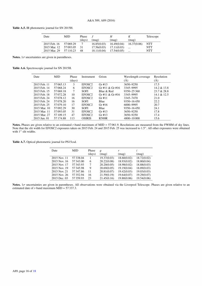
Table A.5. IR photometric journal for SN 2015H.

Date MJD Phase J H K Telescope(days) (mag) (mag) (mag)

2015 Feb. 16 57 069.29 7 16.85(0.03) 16.49(0.04) 16.37(0.06) NTT2015 Mar. 12 57 093.05 31 17.56(0.03) 17.11(0.03) ... NTT2015 Mar. 29 57 110.23 48 18.11(0.04) 17.54(0.05) ... NTT

Notes. 1σ uncertainties are given in parentheses.

Table A.6. Spectroscopic journal for SN 2015H.

Date MJD Phase Instrument Grism Wavelength coverage Resolution(days) (Å) (Å)

2015 Feb. 11 57 065.13 3 EFOSC2 Gr #13 3650–9250 17.52015 Feb. 14 57 068.24 6 EFOSC2 Gr #11 & Gr #16 3345–9995 14.2 & 13.82015 Feb. 15 57 069.18 7 SOFI Blue & Red 9350–25 360 23.7 & 28.82015 Feb. 18 57 072.28 10 EFOSC2 Gr #11 & Gr #16 3345–9995 14.1 & 12.52015 Feb. 24 57 078.12 16 EFOSC2 Gr #11 3345–7470 21.02015 Feb. 24 57 078.20 16 SOFI Blue 9350–16 450 22.22015 Feb. 25 57 079.10 17 EFOSC2 Gr #16 6000–9995 20.72015 Mar. 10 57 092.29 30 SOFI Blue 9350–16 450 24.12015 Mar. 11 57 093.05 31 EFOSC2 Gr #13 3650–9250 17.82015 Mar. 27 57 109.15 47 EFOSC2 Gr #13 3650–9250 17.42015 Jun. 01 57 174.88 113 OSIRIS R500R 4800–10 000 15.6

Notes. Phases are given relative to an estimated r-band maximum of MJD = 57 061.9. Resolutions are measured from the FWHM of sky lines.Note that the slit width for EFOSC2 exposures taken on 2015 Feb. 24 and 2015 Feb. 25 was increased to 1.5′′. All other exposures were obtainedwith 1′′ slit widths.

Table A.7. Optical photometric journal for PS15csd.

Date MJD Phase g r i(days) (mag) (mag) (mag)

2015 Nov. 11 57 338.04 1 19.37(0.03) 18.60(0.02) 18.72(0.02)2015 Nov. 16 57 343.00 6 20.22(0.08) 18.93(0.02) 18.80(0.04)2015 Nov. 17 57 343.93 7 20.20(0.05) 18.98(0.02) 18.88(0.03)2015 Nov. 19 57 345.98 9 20.69(0.05) 19.19(0.04) 18.89(0.03)2015 Nov. 21 57 347.86 11 20.81(0.07) 19.42(0.03) 19.03(0.03)2015 Nov. 26 57 352.94 16 21.59(0.19) 19.64(0.07) 19.29(0.07)2015 Dec. 03 57 359.93 23 21.45(0.16) 19.80(0.06) 19.54(0.06)

Notes. 1σ uncertainties are given in parentheses. All observations were obtained via the Liverpool Telescope. Phases are given relative to anestimated date of r-band maximum MJD = 57 337.3.

A89, page 16 of 18

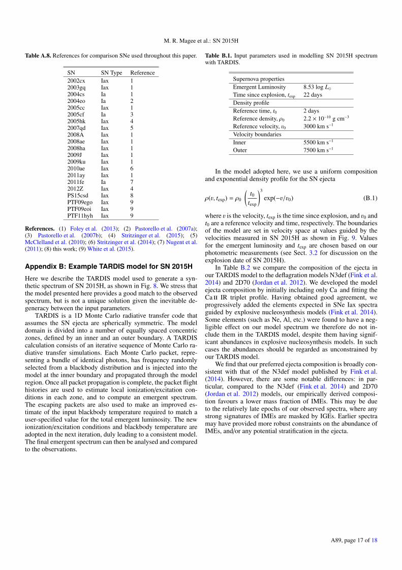
M. R. Magee et al.: SN 2015H

Table A.8. References for comparison SNe used throughout this paper.

SN SN Type Reference2002cx Iax 12003gq Iax 12004cs Ia 12004eo Ia 22005cc Iax 12005cf Ia 32005hk Iax 42007qd Iax 52008A Iax 12008ae Iax 12008ha Iax 12009J Iax 12009ku Iax 12010ae Iax 62011ay Iax 12011fe Ia 72012Z Iax 4PS15csd Iax 8PTF09ego Iax 9PTF09eoi Iax 9PTF11hyh Iax 9

References. (1) Foley et al. (2013); (2) Pastorello et al. (2007a);(3) Pastorello et al. (2007b); (4) Stritzinger et al. (2015); (5)McClelland et al. (2010); (6) Stritzinger et al. (2014); (7) Nugent et al.(2011); (8) this work; (9) White et al. (2015).

Appendix B: Example TARDIS model for SN 2015H

Here we describe the TARDIS model used to generate a syn-thetic spectrum of SN 2015H, as shown in Fig. 8. We stress thatthe model presented here provides a good match to the observedspectrum, but is not a unique solution given the inevitable de-generacy between the input parameters.

TARDIS is a 1D Monte Carlo radiative transfer code thatassumes the SN ejecta are spherically symmetric. The modeldomain is divided into a number of equally spaced concentriczones, defined by an inner and an outer boundary. A TARDIScalculation consists of an iterative sequence of Monte Carlo ra-diative transfer simulations. Each Monte Carlo packet, repre-senting a bundle of identical photons, has frequency randomlyselected from a blackbody distribution and is injected into themodel at the inner boundary and propagated through the modelregion. Once all packet propagation is complete, the packet flighthistories are used to estimate local ionization/excitation con-ditions in each zone, and to compute an emergent spectrum.The escaping packets are also used to make an improved es-timate of the input blackbody temperature required to match auser-specified value for the total emergent luminosity. The newionization/excitation conditions and blackbody temperature areadopted in the next iteration, duly leading to a consistent model.The final emergent spectrum can then be analysed and comparedto the observations.

Table B.1. Input parameters used in modelling SN 2015H spectrumwith TARDIS.

Supernova propertiesEmergent Luminosity 8.53 log L�Time since explosion, texp 22 daysDensity profileReference time, t0 2 daysReference density, ρ0 2.2 × 10−10 g cm−3

Reference velocity, v0 3000 km s−1

Velocity boundariesInner 5500 km s−1

Outer 7500 km s−1

In the model adopted here, we use a uniform compositionand exponential density profile for the SN ejecta

ρ(v, texp) = ρ0

(t0

texp

)3

exp(−v/v0) (B.1)

where v is the velocity, texp is the time since explosion, and v0 andt0 are a reference velocity and time, respectively. The boundariesof the model are set in velocity space at values guided by thevelocities measured in SN 2015H as shown in Fig. 9. Valuesfor the emergent luminosity and texp are chosen based on ourphotometric measurements (see Sect. 3.2 for discussion on theexplosion date of SN 2015H).

In Table B.2 we compare the composition of the ejecta inour TARDIS model to the deflagration models N3def (Fink et al.2014) and 2D70 (Jordan et al. 2012). We developed the modelejecta composition by initially including only Ca and fitting theCa ii IR triplet profile. Having obtained good agreement, weprogressively added the elements expected in SNe Iax spectraguided by explosive nucleosynthesis models (Fink et al. 2014).Some elements (such as Ne, Al, etc.) were found to have a neg-ligible effect on our model spectrum we therefore do not in-clude them in the TARDIS model, despite them having signif-icant abundances in explosive nucleosynthesis models. In suchcases the abundances should be regarded as unconstrained byour TARDIS model.

We find that our preferred ejecta composition is broadly con-sistent with that of the N3def model published by Fink et al.(2014). However, there are some notable differences: in par-ticular, compared to the N3def (Fink et al. 2014) and 2D70(Jordan et al. 2012) models, our empirically derived composi-tion favours a lower mass fraction of IMEs. This may be dueto the relatively late epochs of our observed spectra, where anystrong signatures of IMEs are masked by IGEs. Earlier spectramay have provided more robust constraints on the abundance ofIMEs, and/or any potential stratification in the ejecta.

A89, page 17 of 18

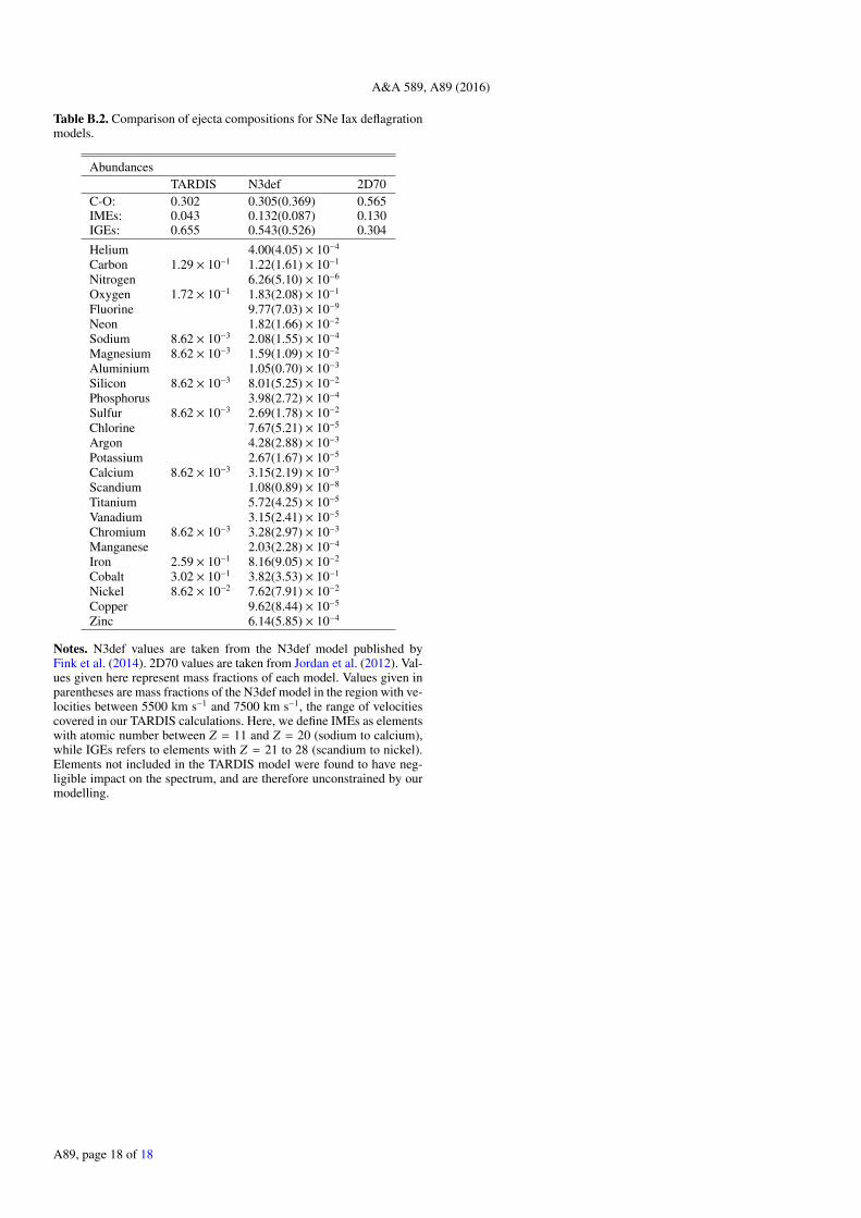
A&A 589, A89 (2016)

Table B.2. Comparison of ejecta compositions for SNe Iax deflagrationmodels.

AbundancesTARDIS N3def 2D70

C-O: 0.302 0.305(0.369) 0.565IMEs: 0.043 0.132(0.087) 0.130IGEs: 0.655 0.543(0.526) 0.304

Helium 4.00(4.05) × 10−4

Carbon 1.29 × 10−1 1.22(1.61) × 10−1

Nitrogen 6.26(5.10) × 10−6

Oxygen 1.72 × 10−1 1.83(2.08) × 10−1

Fluorine 9.77(7.03) × 10−9

Neon 1.82(1.66) × 10−2

Sodium 8.62 × 10−3 2.08(1.55) × 10−4

Magnesium 8.62 × 10−3 1.59(1.09) × 10−2

Aluminium 1.05(0.70) × 10−3

Silicon 8.62 × 10−3 8.01(5.25) × 10−2

Phosphorus 3.98(2.72) × 10−4

Sulfur 8.62 × 10−3 2.69(1.78) × 10−2

Chlorine 7.67(5.21) × 10−5

Argon 4.28(2.88) × 10−3

Potassium 2.67(1.67) × 10−5

Calcium 8.62 × 10−3 3.15(2.19) × 10−3

Scandium 1.08(0.89) × 10−8

Titanium 5.72(4.25) × 10−5

Vanadium 3.15(2.41) × 10−5

Chromium 8.62 × 10−3 3.28(2.97) × 10−3

Manganese 2.03(2.28) × 10−4

Iron 2.59 × 10−1 8.16(9.05) × 10−2

Cobalt 3.02 × 10−1 3.82(3.53) × 10−1

Nickel 8.62 × 10−2 7.62(7.91) × 10−2

Copper 9.62(8.44) × 10−5

Zinc 6.14(5.85) × 10−4

Notes. N3def values are taken from the N3def model published byFink et al. (2014). 2D70 values are taken from Jordan et al. (2012). Val-ues given here represent mass fractions of each model. Values given inparentheses are mass fractions of the N3def model in the region with ve-locities between 5500 km s−1 and 7500 km s−1, the range of velocitiescovered in our TARDIS calculations. Here, we define IMEs as elementswith atomic number between Z = 11 and Z = 20 (sodium to calcium),while IGEs refers to elements with Z = 21 to 28 (scandium to nickel).Elements not included in the TARDIS model were found to have neg-ligible impact on the spectrum, and are therefore unconstrained by ourmodelling.

A89, page 18 of 18