Embed Size (px)
Citation preview
International Journal for Innovation Education and Research www.ijier.net Vol.2-09, 2014
International Educative Research Foundation and Publisher © 2014 pg. 64
The Twin Deficit and the Macroeconomic variables in Kenya
Kennedy O.Osoro
Corresponding author
School of Economics, Unversity of Nairobi
P.O Box 30197-00100, Nairobi- Kenya
Email: [email protected]
Seth O.Gor
School of Economics,University of Nairobi,
Email: [email protected] / [email protected]
and
Mary L.Mbithi
School of Economics,University of Nairobi
Email: [email protected]; [email protected]
Abstract
The purpose of this paper is to test the twin deficit hypothesis and empirical relationship between current
account balance and budget deficit while including other important macroeconomic variables such as growth,
interest rates, money supply (M3) in Kenya from 1963-2012. The study was based on co integration analysis
and error correction model (ECM). The results reveal a long-run association between the trade deficit and the
fiscal deficit. The findings indicate that the Keynesian view fits well for Kenya since the causality runs from
budget deficit to current account deficit. We detected unidirectional causation between the twin deficits,
running from budget deficit to current account directly and indirectly through budget deficits which raise real
interest rates, crowd out domestic investment, and cause the currency to appreciate in relation to the other
currencies and further deteriorates the current account deficit.
Keywords: current account, fiscal balance, co integration, granger causality, Kenya.
1. Introduction
A country is deemed to have a double deficit if it has a current account deficit and a fiscal deficit. Kenya is
likely to experience a persistent double deficit unless fiscal deficit is checked. The country’s fiscal situation
stands at 6.4 per cent of GDP, while that of the current account deficit stands at 10.8 per cent of GDP in 2014.
Large fiscal deficits may lead to currency depreciation or appreciation, and also affect inflation or price levels
which in turn will make interest rates rise. The deficit is likely to grow to become severe if the government
continues to maintain the current huge budget deficit. Therefore the immediate priority of the government is to
contain the fiscal deficit and the current account deficit. The twin deficit hypothesis suggests that when a
government increases its fiscal deficit mostly by cutting taxes or increasing expenditure, domestic residents use
some of the additional income to boost consumption, causing private and public saving to decline. This may
force the country to either borrow from abroad or reduce its foreign lending, unless domestic investment
decreases enough to offset the saving shortfall.
No doubt Kenya has joined countries that have both a fiscal deficit and a current account deficit for years.
International Journal for Innovation Education and Research www.ijier.net Vol.2-09, 2014
International Educative Research Foundation and Publisher © 2014 pg. 65
Current account refers to the sum of the net revenue on exports minus payments for imports of goods and
services, earnings on foreign investments minus payments made to foreign investors and cash transfers. Current
account can be depicted by the following formula:
𝐶𝐴 = 𝐵𝑇 + 𝑁𝐼 + 𝑁𝑇…………………………..1
Where:
CA is the current account; BT is the export and import of goods and services; NI is the net income
from abroad; and NT is the net current transfers.
Current account deficit is therefore the difference between the value of exports of goods and services and the
value of imports of goods and services, net income and transfers from abroad. The current account can also be
expressed as the difference between both public and private savings and investment. Kenya is considered to be
trapped in an excessive debt position for its current account showed substantial deficit except for a few years
during the 1996, 2000 and 2005 when it recorded a surplus of ksh 6228m, ksh7461m, and ksh 1387m
respectively from independence in 1963. Higher current account deficit means higher demand for foreign
currency, which may result in depreciation of the Kenyan currency. It may also discourage capital inflow and
lead to capital flight from the country which would complicate the adjustment process. Therefore the high
current account deficits in recent years have no doubt led to an increase in inflation, exchange rate depreciation
and interest rates rise. As a result the twin deficit problem is magnified due to the presence of higher government
deficit which rendered the current account in a deficit timidly threatening Kenya to be a debtor country in the
long future.
On the other hand, fiscal deficit is used to describe the scenario when a nation's expenses exceed its revenues.
A large budget deficit will spill over to current account deficit through tax cuts or increased spending which
may increase the deficit and reduce revenues, resulting in increased consumption. The increased spending
lowers the national savings rate which increases a nation external borrowing. Therefore, higher fiscal deficit,
apart from affecting savings and growth, affects business confidence. As a result, addressing the issue of twin
deficit will possibly be the biggest policy challenge for the Kenya government.
Thus our study focused on the twin deficits hypothesis in Kenya, and used time-series econometrics
2. Literature review
2.1 Theoretical Literature
Economic theory predicts that a deterioration in the budget balance results in a weakening of the current account.
Therefore we refer to four competing views that explain the association between budget deficit and current
account deficit.
According to the traditional approach or Keynesian absorption approach, when the economy is in a state of full
employment, an increase in budget deficit leads to current account deficit as a result of an increase in aggregate
demand for goods and services, both domestic and imported (Charusheela, 2005). The classical approach to
this issue claims that a substantial and sustained fiscal deficit significantly affects the size of savings and
investments, the prices of production factors, income distribution, exchange rate and the size of foreign trade.
As such the conventional or Keynesian proposition, emphasize that an increase in budget deficit enhances
domestic absorption through greater spending on domestic as well as foreign goods which will reduce exports,
and increase imports, leading to a decline in trade deficit. Therefore the Keynesian proposition can be
summarized to explain, a positive relationship between current account and budget deficit and there exists a
unidirectional Granger causality that runs from the budget deficit to the current account deficit.
International Journal for Innovation Education and Research www.ijier.net Vol.2-09, 2014
International Educative Research Foundation and Publisher © 2014 pg. 66
On the other hand, the Mundell -Fleming model modified the conventional model of twin deficit hypothesis. It
emphasized that increases in the government’s budget deficit leads to an increase in the trade deficit in an open
economy through increased consumer spending. Therefore according to this quantitative approach, high fiscal
deficit leads to higher interest rates which in turn would attract capital inflows and thereby, causing appreciation
in the exchange rate (Cebula, 1988 and 2003; Feldstein, 1986; Rosensweig and Tallman, 1993). This will make
exports to become dearer and imports cheaper, thereby, worsening the trade deficit, under flexible exchange
rate if prices remain constant.
Similarly, Ricardian equivalence approach advanced by Barro (1989) argued that an increase in budget deficits
due to an increase in government spending, must be paid for either now or later, with the total present value of
receipts fixed by the total present value of spending. Thus, a cut in today’s taxes must be matched by an
increase in future taxes, leaving interest rates, and thus private investment, unchanged. Ricardian equivalence
hypothesis (REH) posits that lower public savings are met by equal increases in private savings, and as a result
the current account does not respond to the changes in government spending and consequently to general fiscal
balance.
1. The hypothesis asserts that there is absence of causal relationship between the budget deficit and trade
deficit. This happens as people foresee higher tax liabilities in future, as budgetary deficit expands and
attempt to save more by spending less. Hence, a budget deficit does not result in a widened trade account
deficit (Enders and Lee, 1990).Thus, under Ricardian equivalence hypothesis, the balance of state budget and
the balance of current account are mutually independent or even negatively related (Makin, 2002).
2.2 Empirical evidence
Two forms of causality have been tested in studies of twin deficit hypothesis. They are the Reverse Causality
and Bi-directional Causality. The Reverse Causality view involves unidirectional causality running from current
account deficit to budget deficit. As a result therefore a deteriorated current account reduces the pace of
economic growth. On the other hand, Bi-directional Causality assumption occurs when the two deficits are
mutually dependent and there prevails bi-directional causality between the two deficits.
The twin deficit hypothesis started to attract thoughts in the 1980’s though there were early studies, such as the
one of Milne (1977) and Bernheim (1987) who found positive and statistically significant relationship between
the two deficits using ordinary least squares (OLS) regressions on cross-country data.
The early empirical evidence mainly based on the USA is mixed. Abell (1990) suggested that the hypothesis
holds and indicated that budget deficits impact current account deficits through movements in interest rates and
exchange rates. He used a seven-variable VAR system and data for the period 1979–1985. In contrast, Enders
and Lee (1990 estimated a six variable structural VAR with the differenced data for 1947 to 1985 but did not
find any evidence that budget deficits raise the trade deficit. Kim and Roubini (2008) estimated a VAR in levels
for the post-Bretton- Woods’s period. The results suggested that the U.S. government budget deficits improved
the U.S. current account balance, which is exactly the opposite of what the theoretical model predicts.
Siddiqui (2007) analyzed the relationship between budget deficit and current account deficit in the six countries
of South Asia (Bangladesh, Bhutan, India, Nepal, Pakistan, Sri Lanka) during the period 1960-2004 by using
International Journal for Innovation Education and Research www.ijier.net Vol.2-09, 2014
International Educative Research Foundation and Publisher © 2014 pg. 67
the vector error correction model. The results of analysis indicated the presence of the twin deficits hypothesis
in four of the six examined economies. Similar results were obtained by Lau, Baharumshah and Khalid (2006)
who analyzed the relationship between budget deficit and current account deficits in four Asian countries
(Indonesia, Malaysia, Philippines and Thailand) in the period 1976-2000. The results indicated presence of
long-run relationship between budget deficit and current account deficit. They also confirmed the existence of
the twin deficits hypothesis in the case of Thailand.
Baharumshah, Ismail and Lau (2009) found evidence for the twin deficits hypothesis for Malaysia, Thailand
and Philippines but there was no evidence for Indonesia and Singapore. Similarly Azgun (2012) also found
evidence for the twin deficit hypothesis in context of Turkish economy for the post adoption of economic
reforms in the period 1980-2009.
Marinheiro (2006) examined the relationship between the fiscal deficit and the current account deficit in Egypt
during the period 1974-2002, using a VAR model. The results indicated a one-way influence of the current
account deficit on the fiscal deficit.
Nickel and Vansteenkiste (2008) examined the relationship between the current account and the government
budget balance in 22 industrialized countries in the period 1981- 2005. They found that in very high indebted
countries this relationship was negative but insignificant, suggesting that a rise in the government deficit does
not result in a rise in the current account deficit. Hence, these results suggested that households in indebted
countries tend to become Ricardian.
Vamvoukas (1997) used co-integration analysis, error-correction modeling and Granger causality to evaluate
the validity of both the twin deficit hypothesis and the rational expectations hypothesis for the Greek economy.
The results showed a one-way causality from budget deficit to current account deficit. Additionally the error-
correction modeling evidence supports robustly the twin deficit hypothesis proposition in the short and long
run.
Khalid and Guan (1999) used co-integration analysis to determine the causal relationship between current
account and budget deficits and its direction, using a sample of annual time series data from five developed and
five developing countries. The results from co-integration appear to suggest that a high correspondence between
the two deficits in the long run is more likely to occur in the developing countries than the developed ones.
Results on the Granger test of causality support the existence of a causal relationship between the current
account deficit and the budget deficit in mixed direction for developing countries. The evidence suggests that
current account deficits cause budget deficits for Indonesia and Pakistan, whereas the reverse is true for Egypt
and Mexico. The data does not support any causal relationship for UK and Australia and supports only some
weak evidence of bi-directional causality for Canada and India.
Saleh et al. (2005) tested the twin deficit hypothesis by using autoregressive distributed lag (ARDL) model for
SriLanka. They found a long-run relationship between current account imbalances and budget deficit for the
period 1970 to 2003. Their empirical results also showed that the direction of causality runs from the budget
deficit to the current account deficit. Piersanti (2000), Leach man and Francis (2002) also used the modern
statistical time series technique and found strong evidence to support the Keynesian view.
Kouassi et al. (2004) suggested that the twin deficit hypothesis fitted well for Thailand as the causality ran from
budget deficit to current account deficit. For Indonesia, the causality ran in an opposite direction while the
empirical results indicate that a bidirectional pattern of causality exists for Malaysia and the Philippines. They
International Journal for Innovation Education and Research www.ijier.net Vol.2-09, 2014
International Educative Research Foundation and Publisher © 2014 pg. 68
also found indirect causal relationship runs from budget deficit to higher interest rates, and higher interest rates
leading to the appreciation of the exchange rate, which in turn leads to the widening of the current account
deficit.
Baharumshah et al. (2006) examined the twin deficit hypothesis in the ASEAN countries and found that there
is a long run relationship between budget and current account deficits. They found out that budget deficits lead
to the current account deficit. Lee (1990) and Mohammadi (2004) found that the increase of budget surplus/GDP
ratio by one percent improves the current account/GDP ratio by 0.31 to 0.49 percent in developing countries.
Hoelscher (1986) and Cebula and Koch (1989), concluded that Federal budget deficits contributed to higher
levels of interest rate yields. Knoester and Mak (1994) showed that only in Germany (among eight OECD
economies) did the government budget deficit contribute to explain of higher interest rates. Abell (1990) showed
that the link between the two deficits is indirect. Fieleke (1987), found that an increase in government borrowing
lead to increase in interest rate other things being equal.
Chaudhry and Shabbir (2005), in their study tried to show the impact of budget deficit on money supply, foreign
reserve and balance of payments. They used the annual data for the period 1965-1999 and the 2SLS technique
and they concluded that changes in money supply affect the trade balance through output.
3. Methodology
Our paper is built on two strands of literature: the literature on the conventional or Keynesian proposition and
the literature on the Mundell- Fleming model to test the two hypotheses. We start the analysis of the twin deficit
hypothesis with a review of a basic national accounting identity. We begin by relating the external deficit to the
difference between national investment and national saving, which in turn is the sum of private and public
saving. This is because a fall in national saving due to a government deficit other things kept constant lead into
a fall in the current account balance.
3.1 Empirical model
We start by clarifying the relationship between the balance of government budget and the balance of current
account, using the national income identity expressed as:
Y = C + I + G + (X - M) …………………………………………….. (2)
Where:
Y is the national income; C is the private consumption; I is investment expenditures;
G is government expenditure; X is exports of goods and services; M is imports of goods and services.
Given that
Y= C+I+G+NX and Y-C-T=S, then S=G-T+NX+I,
which if simplified come to:
(S-I) + (T-G) = (NX) …………………………………………… (3)
Where:

International Journal for Innovation Education and Research www.ijier.net Vol.2-09, 2014
International Educative Research Foundation and Publisher © 2014 pg. 69
S= Saving and T=Taxes.
If (T-G) is negative, we have a budget deficit.
On the other hand, current account balance can be represented by the following expression:
S = Y - C - G + CA or S = I + CA …………………………....(4)
Where: I is investment.
Starting with the national income equation, national savings in an open economy can then be express as: S.
We can also express the national income equation, whereby investments can be expressed by the formula:
I = Y - C - G ……………………………………………………(5)
National savings comprise private sector saving (Sp) and public sector saving (Sg). Thus:
S = Sp + Sg
Whereby: private savings are the part of personal disposable income which is not consumed and can be re
written as:
Sp =Yd -C = (Y- T) –C ……………………………………….. (6)
Where:
Yd is the disposable personal income; and T is Taxes.
While public savings are the difference between the government revenue (taxes) and budget expenditures,
which include government purchases (G) and government transfers (R), which can be written as:
Sg= T - (G+ R) =T -G -R ……………………………………….. (7)
Thus, national saving (s) can be expressed as:
S = [Sp+ Sg] = (Y -T -C) + (T -G -R)] = I+ CA ………………….(8)
If: S=I+CA; then, finally, current account balance can be presented in the form of:
CA =Sp- I - (G+ R -T)……………………………………………(9)
This shows that, if there is constant difference between private savings and investments, then the fiscal balance
changes are reflected in the changes in the balance of current account, an indication of twin deficits hypothesis.
This situation results from the fact that the increase in budget deficit leads to an increase in national savings due
to the expected increase in taxes in the future, which in turn does not lead to an increase in consumer spending
and to the deficit of current account.
The twin deficits hypothesis asserts that an increase in budget deficit will cause similar increase in current
account deficit and vice versa. Theoretically the mechanism behind the twin deficits could also simply be
explained through the Keynesian income-expenditure approach. An increase in budget deficit will cause an
increase in domestic absorption, and therefore the domestic income. When the domestic income increases, it
will encourage imports and eventually will reduce the surplus in the trade balance. In addition, the Keynesian
International Journal for Innovation Education and Research www.ijier.net Vol.2-09, 2014
International Educative Research Foundation and Publisher © 2014 pg. 70
open economy model states that an increase in the budget deficit will cause an increase in the aggregate demand
and domestic real interest rates. High interest rates will lead to net capital inflow and result in appreciation of
domestic currency. Higher value of the domestic currency will then adversely affect net exports, and thus there
will be worsening in the current account deficit.
The historical statistical data from independent showed that Kenya is experiencing fiscal deficits or ‘government
deficit, except for the year of 1973, and 1998-2001. The Kenya current account balances are in surpluses for
only the year of 1970, 1973-76, 1980-81, and 1991.
We therefore developed a general model for estimation based on the theory:
𝐶𝐴𝐷 = 𝑓(𝐷𝐸𝐹, 𝐼𝑁𝑇, 𝐺𝐷𝑃, 𝑀𝑂𝑁) … … … … … … … … … … … … … … … . .10
Our estimated model is presented as:
𝐶𝐴𝐷 = 𝑓(𝛽0 + 𝛽1 𝐷𝐸𝐹 + 𝛽2𝐼𝑁𝑇 + 𝛽3𝐺𝐷𝑃 + 𝛽4𝑀𝑂𝑁) + 𝑡 … … … … … … … 11
Where:
CAD is the current account measured in US dollar; DEF is fiscal deficit measured in US dollar; INT is
interest rates; GDP is nominal GDP; MON is money supply measured in US dollar and; t is Error
term.
Thus in the analysis, we extend the bivariate model to include interest rates, nominal GDP and money supply.
3.2 Data types and sources
All the data used in this study, were obtained from several International Financial Statistics (IFS) issues
published by the International Monetary Fund (IMF), Kenya’s economic surveys various, and statistical
Abstracts. The variables employed in the study were the current account (CAD), budgetary deficit, interest rate,
nominal GDP and money supply.
3.3 Unit root tests and Co integration Analysis
We utilized the Johansen and Juselius (1990) maximum likelihood co integration test and granger causality in
identifying the linkage between the twin deficits. Pair wise causality test and Error Correction Model (ECM)
technique were applied on annual budget deficit and current account deficit. The Johansen test permits the
identification of multiple co integration relationships.
Then Johansen technique is based on a VAR model with k lags as:
Yt=A1*yt-1+ A2*yt-2……..+ AK*yt-k+ εt ……………………………(12)
Where:
Yt is a vector (n x 1); Ai is the parameters matrix (n x n).
We transformed the VAR into an error correction mechanism, and obtained:
ΔYt = Γ1Δyt-1 + …. +Γ1Δyt-k+1 + Π yt-k + εt ……………………….(13)
Where:
Γi=-(I-A1-…-Ai), i=1, k −1; Π=-(I-A1-…-Ak), Π=αβ’,
International Journal for Innovation Education and Research www.ijier.net Vol.2-09, 2014
International Educative Research Foundation and Publisher © 2014 pg. 71
α - represents the speed of adjustment and β the matrix of long-run coefficients. The number of the co
integrating relationships is given by the rank of Π.
4. Results and discussion
Detailed results of all the analysis are found in annexes 1-10.
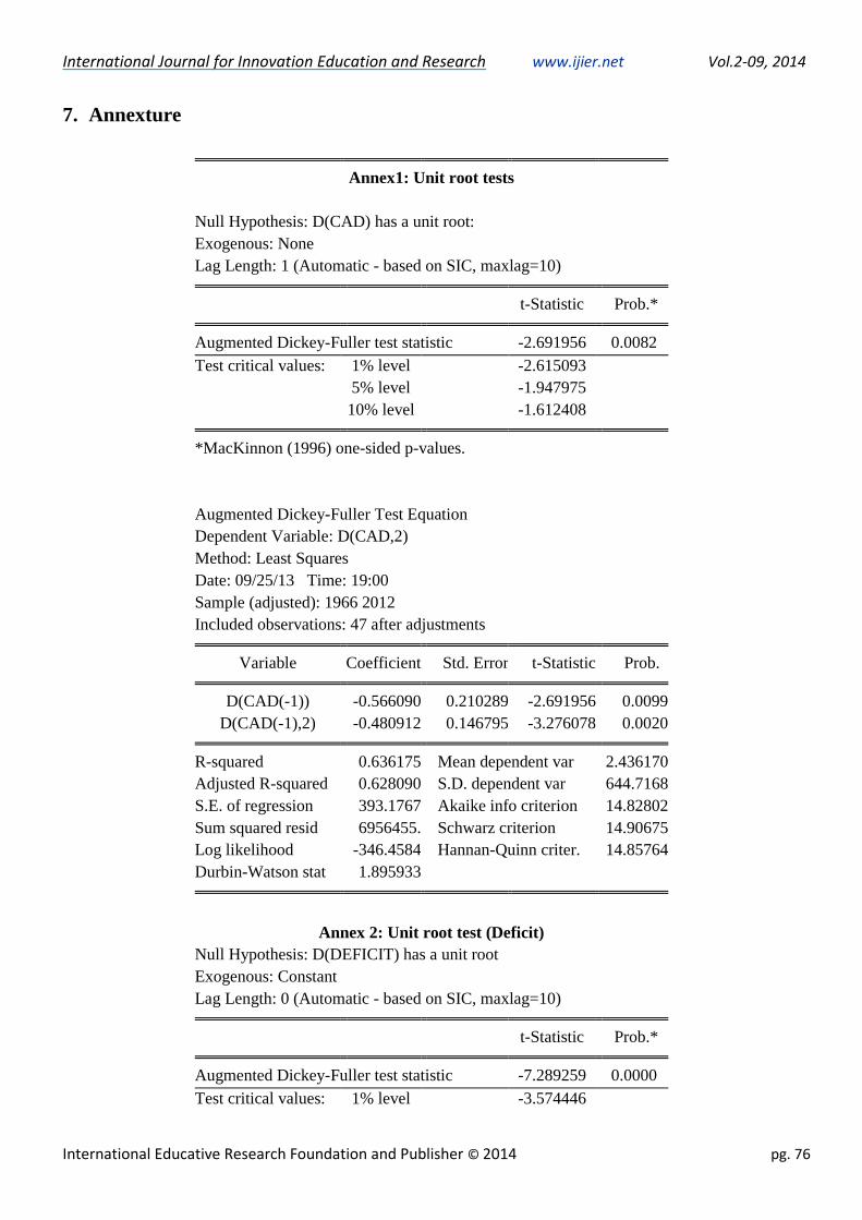
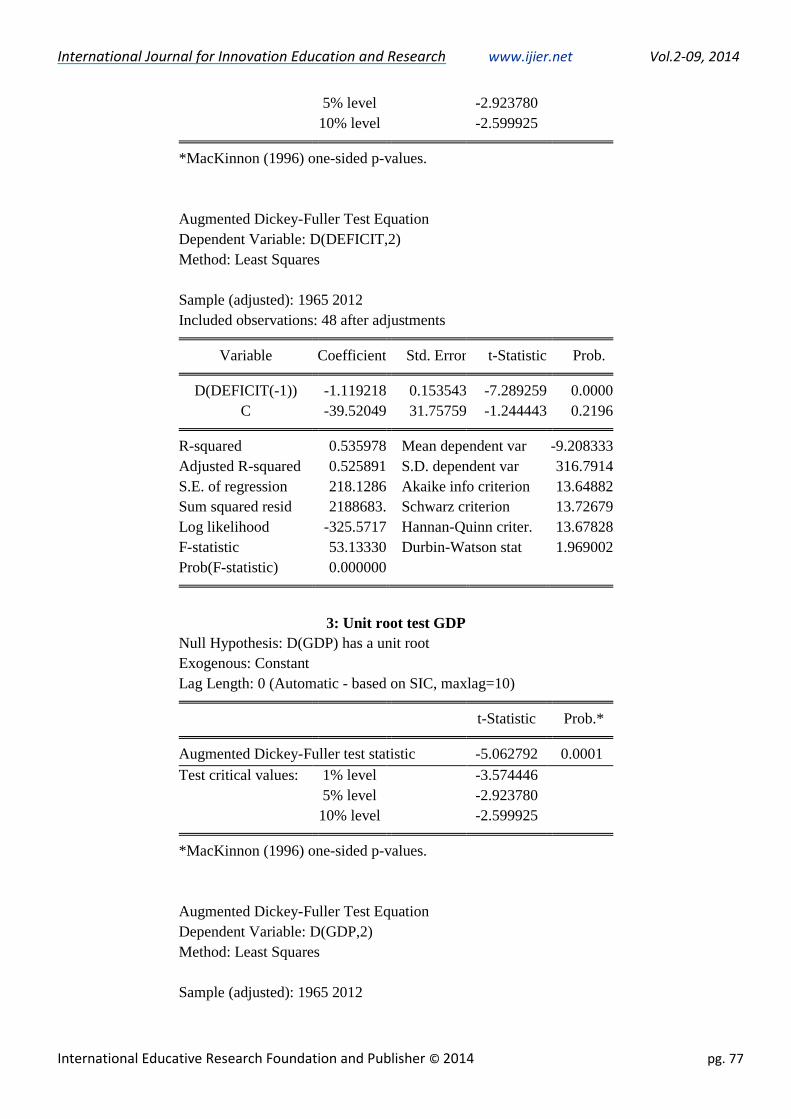
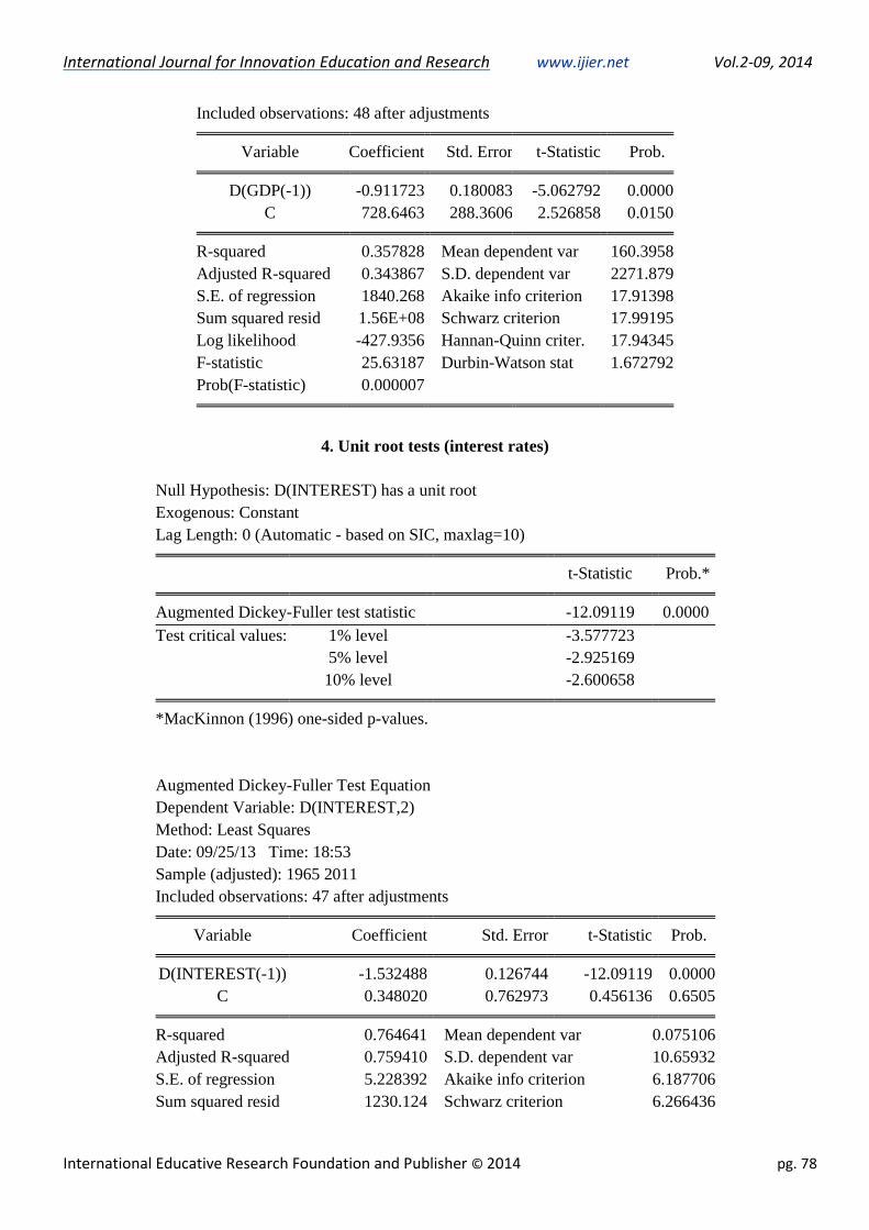
4.1. Results of Augmented Dickey Fuller test
Table 1 presents the results of Augmented Dickey Fuller (ADF) test. The ADF statistics confirmed that all the
variables (trade deficit, budget deficit, interest rate money supply and gross domestic product) were not
stationary at levels. However they became stationary after first difference indicating that they were integrated
of order one i.e. I (1), an indication of a significant co-integration relationship among the variables. The ADF
results shown in Table 1 suggested that all the variables are found to be non-stationary in level but were
stationary in first difference at 5% level of significance.
Table 1: ADF test of nonstationarity hypothesis
Variable
test
critical
at levels
test
critical
at 5%
test critical
first
difference
test critical
at 5%
probability
CAD -2.087 -2.925 -2.692 -1.948 0.008
DEF 0.116 -2.922 -7.289 -2.928 0.000
GDP 1.321 -3.504 -5.063 -2.928 0.000
MON 0.101 -2.929 -3.998 -2.925 0.003
INT -1.728 -2.925 -12.091 -2.925 0.000
U (-1) error term -6.243 -3.574 stationary at levels 0.000
Source: Authors
The second step in the empirical analysis was to test for co integration among the variables to detect any possible
long-run equilibrium between the series. The results of the Johansen co integration test are influenced by the
considered lag length. Therefore the lag length was chosen using various criteria including the Akaike
Information Criteria (AIC), LR (Likelihood Ratio Criterion), SIC (Schwarz Information Criterion), FPE (Final
Prediction Error) and HQ (Hannan-Quinn Information Criterion) . The results of lag length selection are
presented in Table 2.
Table 2. VAR lag order selection criteria
Lag LogL LR FPE AIC SC HQ
0 -1728.202 NA 3.67e+26 75.35661 75.55537 75.43107
1 -1567.939 278.7176 1.03e+24 69.47562 70.66822* 69.92238
2 -1531.817 54.96872 6.62e+23 68.99205 71.17846 69.81109
3 -1505.406 34.44901 6.91e+23 68.93070 72.11095 70.12204
4 -1448.887 61.43363* 2.17e+23* 67.56031* 71.73439 69.12395*
Source: Authors
International Journal for Innovation Education and Research www.ijier.net Vol.2-09, 2014
International Educative Research Foundation and Publisher © 2014 pg. 72
* indicates lag order selected by the criterion
LR is the sequential modified LR test statistic (each test at 5% level)
FPE is the final prediction error
AIC is the Akaike information criterion
SC is the Schwarz information criterion
HQ is the Hannan-Quinn information criterion.
The maximum lag length for GDP, Money supply and government deficit is four periods according to LR,
FPE, AIC and HQ criteria.
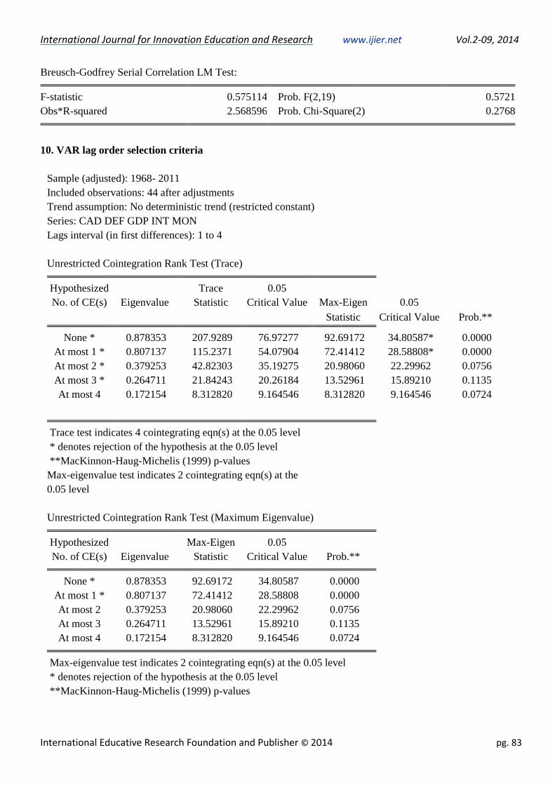
In the third step we proceeded to run the co integration tests which showed that Kenya’s fiscal balance, current
account balance, nominal GDP and interest rates (short- and long-run) were co-moved over the periods, as
shown in Table 3.
Table 3: Unrestricted Co integration Rank Test (Trace)
Hypothesized Trace 0.05
No. of CE(s)
Eigen
value Statistic
Critical
Value Max-Eigen 0.05
Statistic Critical Value Prob.**
None * 0.878353 207.9289 76.97277 92.69172 34.80587* 0.0000
At most 1 * 0.807137 115.2371 54.07904 72.41412 28.58808* 0.0000
At most 2 * 0.379253 42.82303 35.19275 20.98060 22.29962 0.0756
At most 3 * 0.264711 21.84243 20.26184 13.52961 15.89210 0.1135
At most 4 0.172154 8.312820 9.164546 8.312820 9.164546 0.0724
Source: Authors
Trace test indicates for 3 co integrating eqn (s) at the 0.05 level
* denotes rejection of the hypothesis at the 0.05 level
**MacKinnon-Haug-Michelis (1999) p-values
Max-eigen value test indicates 2 co integrating eqn (s) at the 0.05 level
The results in Table 3 indicate four and two co integration equations by trace statistics and Max-Eigen statistics.
This suggests that there exists a long-run equilibrium relationship binding all these variables. The equilibrium
mechanism then was established through two major channels whereby budget deficit affects the current account
in the country. The first one we established was a direct causal link from budget deficit to current account
deficit, and the other was the indirect channel that runs from budget deficit to higher interest rate; higher interest
rates lead to appreciation of the currency and this in turn worsens the current account deficit.
4.2 Results on granger causality tests
Determination on whether or not fiscal deficits Granger cause exchange rates and other variables and vice-versa,
using Vector Error Correction Model (VECM). In the presence of co integration, there exists an error correction
representation, which captures the deviation or disequilibrium from long-run equilibrium. The disequilibrium
is corrected gradually through a series of partial short-run adjustments.
International Journal for Innovation Education and Research www.ijier.net Vol.2-09, 2014
International Educative Research Foundation and Publisher © 2014 pg. 73
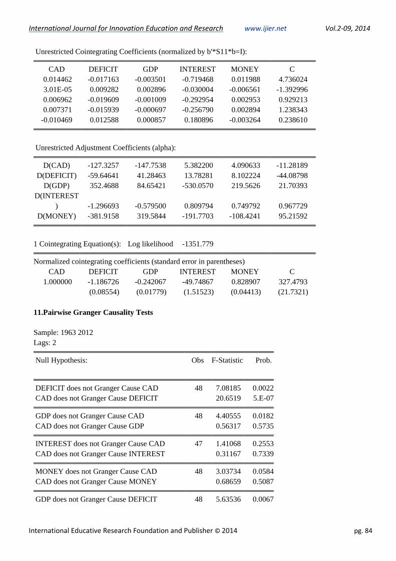
Our findings show that there is a unidirectional causality running from budgetary to current account. The
estimated co integrating equation is:
CAD = -299.033+1.8585 DEF + 0.24206GDP + 49.7560 INT - 0.82922 MON ……….(14)
The signs of the normalized co integrating coefficients indicate two points: First, there is a positive relation
between current account deficit and fiscal deficit, GDP and interest rates. Second, money supply growth exerts
a negative impact on CAD. In other words, current account deficit tends to increase along with the increase in
fiscal deficit, GDP and interest rate in the long run. The coefficients of the error correction have the expected
negative sign and are less than unity. The coefficient of the speed of adjustment (see annex 8) for the error term
of about - 0.8, implying that the model corrects by about 80 percent of the disequilibrium in the short run will
be corrected each year.
The results from granger causality tests are reported in Annex 10. There existed bidirectional causality between
GDP and fiscal deficit. Also a unidirectional causality is found between GDP and CAD, which runs from GDP
to CAD and bidirectional relation between money and fiscal deficit. In the overall, the empirical results support
the existence of a co integrating relation among the variables and the twin deficits hypothesis in Kenya. Its
effect on the current account deficit is positive and significant. Its likely mechanism is through the interest rate,
a monetary expansion leads to an interest rate drop, which in turn encourages investment and, in the absence of
an important saving effect, a rise in the current account deficit.
An increase in the domestic output (GDP) has the effect of enlarging the current account deficit. A 1 percentage
point rise in the GDP growth rate leads to an increase of about 24.2 percentage increase in the current account
deficit.
According to our estimates, a rise in real interest rates of 1 percentage point leads to a current account deficit
increase of about 49.8 percentage points the findings are consistent with the Feldstein chain). Both GDP and
interest rates have a positive impact on a country’s current account balance by either households’ saving
behaviour or investors’ decision to invest. Also, there is a statistically significant negative and stable relationship
between money supply and the current account balance. The results show that a decrease in the money supply
by one percentage point improves the current account balance by 82.8 percentage points. So money supply does
increase whenever we try to finance budget deficit through Government, private or external borrowing.
5. Conclusions and policy implications
We concluded that Keynesian view fits well for Kenya since the causality runs from budget deficit to current
account deficit .The results showed a positive and significant relationship between budget deficit and current
account. The signs of the normalized co integrating coefficients suggest that there is also a positive relationship
between current account deficit and interest rates, GDP and negatively related to money supply. In other words,
current account deficit tends to increase along with the increase in fiscal deficit, GDP, interest rates and decrease
with money supply in the long run. This means, a rise in budget deficit would be followed by an increase in
external balance. We find the causal relationship works through two channels: first is the direct causal link from
budget deficit to current account deficit, and the second is the indirect channel that runs from budget deficit to
higher interest rate; which lead to appreciation of the currency, in turn worsening the current account deficit.
Interest rates seem to cause current account deficits through the exchange rate. So we suggest Kenya to embrace
on a flexible exchange rate regime, higher degree of openness, export diversification, development of the
financial sector, and adopt sound fiscal and monetary policies to improve on the twin deficit.
International Journal for Innovation Education and Research www.ijier.net Vol.2-09, 2014
International Educative Research Foundation and Publisher © 2014 pg. 74
6. References
Abell J. D. (1990), Twin Deficits during the 1980s: An Empirical Investigation, “Journal of Macroeconomics”,
12(1) 81-96.
Barro R. J. (1989), “The Ricardian Approach to Budget Deficits”, Journal of Economic Perspectives, 3 (2), 37-
54.
Baharumshah A. Z., Ismail, H. and Lau, E. (2009), “Twin Deficit Hypothesis and Capital Mobility: The ASEAN
– 5 Perspective”, Journal Pengurusan.
Baharumshah, A. Z., Lau, E. and Khalid, A. M. (2006), “Testing Twin Deficits Hypothesis Using VARs and
Variance Decomposition”, Journal of the Asia Pacific economy, 11 (3),331-354.
Bernheim B.D (1987) “Budget Deficits and the Balance of Trade”, NBER Macroeconomic Annual.
Baharumshah A. Z., Lau, E. and Khalid, A. M. (2006) 'Testing Twin Deficits Hypothesis using VARs and
Variance Decomposition', Journal of the Asia Pacific Economy, 11, (3), pp. 331-354.
Cebula, R. (1988). Federal government deficits and interests in the US: A brief note.
Southern Economic Journal, 55(1), 206–210.
Cebula R.J. and Koch J.V (1989). “An empirical note on deficits, interest rates, and international capital flows”.
The Quarterly Review of Economics and Business, 29(1), pp.119-26
Charusheela S. (2005), Structuralism and Individualism in Economic Analysis, Routledge, New York.
Christiane Nickel and Isabel Vansteenkiste (2008). ―Fiscal Policies, The Current Account and Ricardian
Equivalence‖ Working Paper Series No. 935.
Chaudhary M.A and Shabbir (2005) “Macroeconomic impacts of budget deficit on Pakistan
foreign sector”. Pak Economy and Social Review, xliii (2).
Enders W and Lee BS(1990)"Current Account and Budget Deficits: Twins or Distant
Cousins?". Review of Economics and Statistics, pp. 373-81.
Fieleke N, S (1987). “The budget deficit: are the international consequences unfavorable?”
International university press of America, 171-180
Feldstein M (1986) “The Budget Deficit and the Dollar” in NBER Macroeconomic Annual,
Fleming J. M. (1962), Domestic Financial Policies under Fixed and under Floating Exchange Rates,
“International Monetary Fund Staff Papers”, No 9.
Hoelscher, G.(1986). “New evidence on deficits and interest rates”, Journal of Money, Credit, and Banking,
18(1), pp.1-17.

International Journal for Innovation Education and Research www.ijier.net Vol.2-09, 2014
International Educative Research Foundation and Publisher © 2014 pg. 75
Kouassi E, Mougoue, M. and Kymn, K. O. (2004) 'Causality tests of the relationship between the twin deficits',
Empirical Economics, 29, (3), pp. 503-525.
Khalid A. M. and Guan, T. W. (1999) 'Causality tests of budget and current account deficits: Cross-country
comparisons', Empirical Economics, 24, (3), pp. 389.
Kim S. and Roubini N. (2008). Twin deficit or twin divergence? Fiscal policy, current account and real exchange
rate in the US. Journal of International Economics, 74, 362-383
An Econometric Analysis', South Asia Economic Journal, 6, (2), pp. 221-239.
Knoester, A. and Mak, W.(1994). “Real interest rates in eight OECD countries”. Rivista Internazionale, 41(4),
pp.325-44.
Leachman L. L. and Francis B. (2002) Twin deficits: apparition or reality? Applied Economics, 34, pp. 1121–
1132.
Mohammadi H. (2004) 'budget deficits and the current account balance: new evidence from panel data', Journal
of Economics & Finance, 28, (1), pp. 39-45.
Makin A.J. (2002), International macroeconomics, Pearson Education Limited, London.
Marinheiro C.F. (2006), Ricardian Equivalence, Twin Deficits, and the Feldstein-Horioki
puzzle in Egypt, “Publicacao Co-Financiada Pela Fundacao Para A Ciencia E Tecnologia
Estudos do Gemf”, No 7.
Milne E (1977), The fiscal approach to the balance of payments, Economic Notes, 1, pp. 89 – 107.
Mundell, Robert A. (1963). Capital Mobility and Stabilization Policy Under Fixed and
Flexible Exchange Rates. Canadian Journal of Economics and Political Science
29, 475-85.
Piersanti G.(2000) “Current Account Dynamics and Expected Future Budget Deficits: Some International
Evidence.” Journal of International Money and Finance 19, no. 2: 2555-71.
Rosensweig, Jeffrey and Tallman, Ellis W.(1993) "Fiscal Policy and Trade Adjustment: Are the Deficits Really
Twins?", Economic Inquiry, pp. 580-594.
Saleh A. S., Nair, M. and Agalewatte, T. (2005) 'The Twin Deficits Problem in Sri Lanka:
Siddiqui A. (2007), India and South Asia Economic Developments in the Age of Globalization, M.E. Sharpe,
New York.
Vamvoukas G. A. (1997) 'Have large budget deficits caused increasing trade', Atlantic Economic Journal, 25,
(1), pp. 80.
International Journal for Innovation Education and Research www.ijier.net Vol.2-09, 2014
International Educative Research Foundation and Publisher © 2014 pg. 76
7. Annexture
Annex1: Unit root tests
Null Hypothesis: D(CAD) has a unit root:
Exogenous: None
Lag Length: 1 (Automatic - based on SIC, maxlag=10)
t-Statistic Prob.*
Augmented Dickey-Fuller test statistic -2.691956 0.0082
Test critical values: 1% level -2.615093
5% level -1.947975
10% level -1.612408
*MacKinnon (1996) one-sided p-values.
Augmented Dickey-Fuller Test Equation
Dependent Variable: D(CAD,2)
Method: Least Squares
Date: 09/25/13 Time: 19:00
Sample (adjusted): 1966 2012
Included observations: 47 after adjustments
Variable Coefficient Std. Error t-Statistic Prob.
D(CAD(-1)) -0.566090 0.210289 -2.691956 0.0099
D(CAD(-1),2) -0.480912 0.146795 -3.276078 0.0020
R-squared 0.636175 Mean dependent var 2.436170
Adjusted R-squared 0.628090 S.D. dependent var 644.7168
S.E. of regression 393.1767 Akaike info criterion 14.82802
Sum squared resid 6956455. Schwarz criterion 14.90675
Log likelihood -346.4584 Hannan-Quinn criter. 14.85764
Durbin-Watson stat 1.895933
Annex 2: Unit root test (Deficit)
Null Hypothesis: D(DEFICIT) has a unit root
Exogenous: Constant
Lag Length: 0 (Automatic - based on SIC, maxlag=10)
t-Statistic Prob.*
Augmented Dickey-Fuller test statistic -7.289259 0.0000
Test critical values: 1% level -3.574446
International Journal for Innovation Education and Research www.ijier.net Vol.2-09, 2014
International Educative Research Foundation and Publisher © 2014 pg. 77
5% level -2.923780
10% level -2.599925
*MacKinnon (1996) one-sided p-values.
Augmented Dickey-Fuller Test Equation
Dependent Variable: D(DEFICIT,2)
Method: Least Squares
Sample (adjusted): 1965 2012
Included observations: 48 after adjustments
Variable Coefficient Std. Error t-Statistic Prob.
D(DEFICIT(-1)) -1.119218 0.153543 -7.289259 0.0000
C -39.52049 31.75759 -1.244443 0.2196
R-squared 0.535978 Mean dependent var -9.208333
Adjusted R-squared 0.525891 S.D. dependent var 316.7914
S.E. of regression 218.1286 Akaike info criterion 13.64882
Sum squared resid 2188683. Schwarz criterion 13.72679
Log likelihood -325.5717 Hannan-Quinn criter. 13.67828
F-statistic 53.13330 Durbin-Watson stat 1.969002
Prob(F-statistic) 0.000000
3: Unit root test GDP
Null Hypothesis: D(GDP) has a unit root
Exogenous: Constant
Lag Length: 0 (Automatic - based on SIC, maxlag=10)
t-Statistic Prob.*
Augmented Dickey-Fuller test statistic -5.062792 0.0001
Test critical values: 1% level -3.574446
5% level -2.923780
10% level -2.599925
*MacKinnon (1996) one-sided p-values.
Augmented Dickey-Fuller Test Equation
Dependent Variable: D(GDP,2)
Method: Least Squares
Sample (adjusted): 1965 2012
International Journal for Innovation Education and Research www.ijier.net Vol.2-09, 2014
International Educative Research Foundation and Publisher © 2014 pg. 78
Included observations: 48 after adjustments
Variable Coefficient Std. Error t-Statistic Prob.
D(GDP(-1)) -0.911723 0.180083 -5.062792 0.0000
C 728.6463 288.3606 2.526858 0.0150
R-squared 0.357828 Mean dependent var 160.3958
Adjusted R-squared 0.343867 S.D. dependent var 2271.879
S.E. of regression 1840.268 Akaike info criterion 17.91398
Sum squared resid 1.56E+08 Schwarz criterion 17.99195
Log likelihood -427.9356 Hannan-Quinn criter. 17.94345
F-statistic 25.63187 Durbin-Watson stat 1.672792
Prob(F-statistic) 0.000007
4. Unit root tests (interest rates)
Null Hypothesis: D(INTEREST) has a unit root
Exogenous: Constant
Lag Length: 0 (Automatic - based on SIC, maxlag=10)
t-Statistic Prob.*
Augmented Dickey-Fuller test statistic -12.09119 0.0000
Test critical values: 1% level -3.577723
5% level -2.925169
10% level -2.600658
*MacKinnon (1996) one-sided p-values.
Augmented Dickey-Fuller Test Equation
Dependent Variable: D(INTEREST,2)
Method: Least Squares
Date: 09/25/13 Time: 18:53
Sample (adjusted): 1965 2011
Included observations: 47 after adjustments
Variable Coefficient Std. Error t-Statistic Prob.
D(INTEREST(-1)) -1.532488 0.126744 -12.09119 0.0000
C 0.348020 0.762973 0.456136 0.6505
R-squared 0.764641 Mean dependent var 0.075106
Adjusted R-squared 0.759410 S.D. dependent var 10.65932
S.E. of regression 5.228392 Akaike info criterion 6.187706
Sum squared resid 1230.124 Schwarz criterion 6.266436
International Journal for Innovation Education and Research www.ijier.net Vol.2-09, 2014
International Educative Research Foundation and Publisher © 2014 pg. 79
Log likelihood -143.4111 Hannan-Quinn criter. 6.217332
F-statistic 146.1969 Durbin-Watson stat 2.291625
Prob(F-statistic) 0.000000
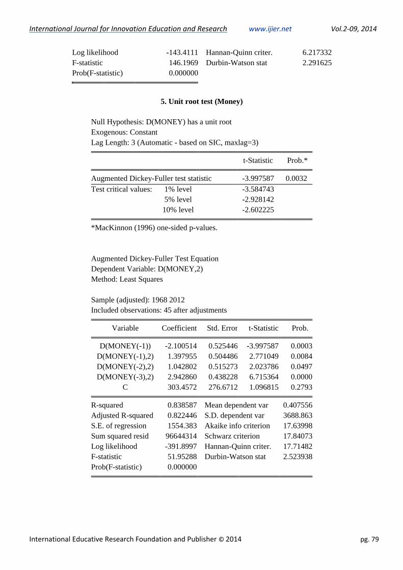
5. Unit root test (Money)
Null Hypothesis: D(MONEY) has a unit root
Exogenous: Constant
Lag Length: 3 (Automatic - based on SIC, maxlag=3)
t-Statistic Prob.*
Augmented Dickey-Fuller test statistic -3.997587 0.0032
Test critical values: 1% level -3.584743
5% level -2.928142
10% level -2.602225
*MacKinnon (1996) one-sided p-values.
Augmented Dickey-Fuller Test Equation
Dependent Variable: D(MONEY,2)
Method: Least Squares
Sample (adjusted): 1968 2012
Included observations: 45 after adjustments
Variable Coefficient Std. Error t-Statistic Prob.
D(MONEY(-1)) -2.100514 0.525446 -3.997587 0.0003
D(MONEY(-1),2) 1.397955 0.504486 2.771049 0.0084
D(MONEY(-2),2) 1.042802 0.515273 2.023786 0.0497
D(MONEY(-3),2) 2.942860 0.438228 6.715364 0.0000
C 303.4572 276.6712 1.096815 0.2793
R-squared 0.838587 Mean dependent var 0.407556
Adjusted R-squared 0.822446 S.D. dependent var 3688.863
S.E. of regression 1554.383 Akaike info criterion 17.63998
Sum squared resid 96644314 Schwarz criterion 17.84073
Log likelihood -391.8997 Hannan-Quinn criter. 17.71482
F-statistic 51.95288 Durbin-Watson stat 2.523938
Prob(F-statistic) 0.000000
International Journal for Innovation Education and Research www.ijier.net Vol.2-09, 2014
International Educative Research Foundation and Publisher © 2014 pg. 80
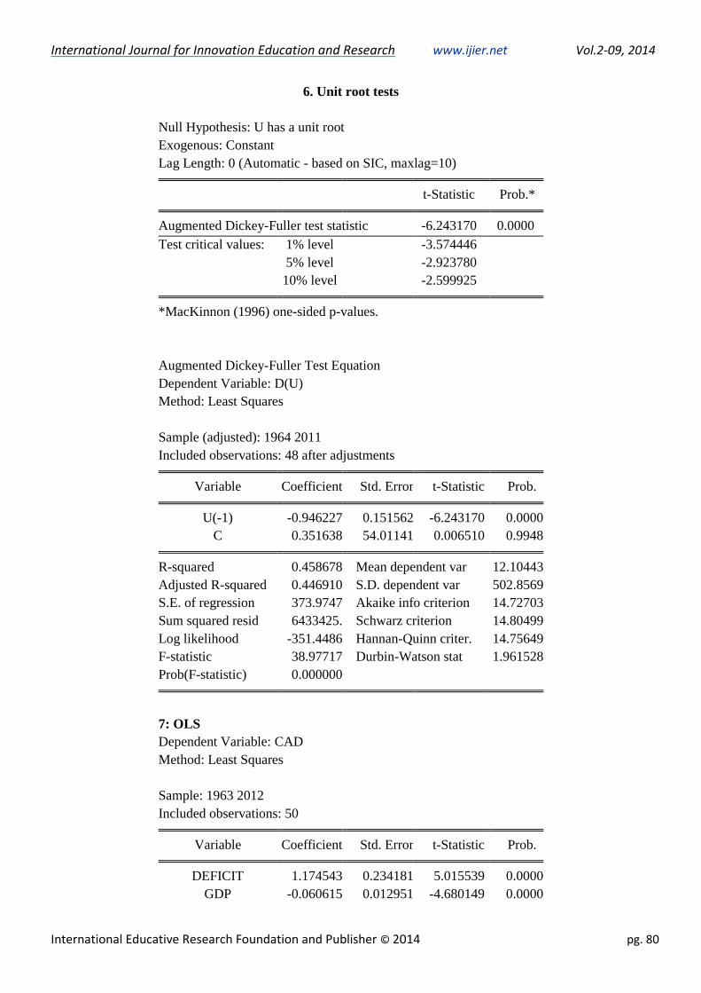
6. Unit root tests
Null Hypothesis: U has a unit root
Exogenous: Constant
Lag Length: 0 (Automatic - based on SIC, maxlag=10)
t-Statistic Prob.*
Augmented Dickey-Fuller test statistic -6.243170 0.0000
Test critical values: 1% level -3.574446
5% level -2.923780
10% level -2.599925
*MacKinnon (1996) one-sided p-values.
Augmented Dickey-Fuller Test Equation
Dependent Variable: D(U)
Method: Least Squares
Sample (adjusted): 1964 2011
Included observations: 48 after adjustments
Variable Coefficient Std. Error t-Statistic Prob.
U(-1) -0.946227 0.151562 -6.243170 0.0000
C 0.351638 54.01141 0.006510 0.9948
R-squared 0.458678 Mean dependent var 12.10443
Adjusted R-squared 0.446910 S.D. dependent var 502.8569
S.E. of regression 373.9747 Akaike info criterion 14.72703
Sum squared resid 6433425. Schwarz criterion 14.80499
Log likelihood -351.4486 Hannan-Quinn criter. 14.75649
F-statistic 38.97717 Durbin-Watson stat 1.961528
Prob(F-statistic) 0.000000
7: OLS
Dependent Variable: CAD
Method: Least Squares
Sample: 1963 2012
Included observations: 50
Variable Coefficient Std. Error t-Statistic Prob.
DEFICIT 1.174543 0.234181 5.015539 0.0000
GDP -0.060615 0.012951 -4.680149 0.0000
International Journal for Innovation Education and Research www.ijier.net Vol.2-09, 2014
International Educative Research Foundation and Publisher © 2014 pg. 81
INTEREST 33.68432 7.315676 4.604403 0.0000
MONEY -0.094996 0.021625 -4.392974 0.0001
C 61.02026 114.7689 0.531679 0.5976
R-squared 0.917243 Mean dependent var -751.5820
Adjusted R-squared 0.909886 S.D. dependent var 1266.763
S.E. of regression 380.2686 Akaike info criterion 14.81427
Sum squared resid 6507190. Schwarz criterion 15.00547
Log likelihood -365.3568 Hannan-Quinn criter. 14.88708
F-statistic 124.6895 Durbin-Watson stat 1.872535
Prob(F-statistic) 0.000000
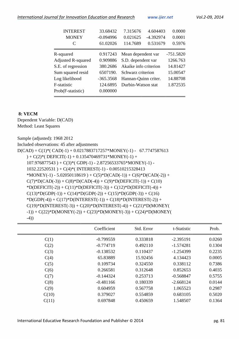
8: VECM
Dependent Variable: D(CAD)
Method: Least Squares
Sample (adjusted): 1968 2012
Included observations: 45 after adjustments
D(CAD) = C(1)*( CAD(-1) + 0.0217883717257*MONEY(-1) - 67.7747587613
) + C(2)*( DEFICIT(-1) + 0.135470469731*MONEY(-1) +
107.976877543 ) + C(3)*( GDP(-1) - 2.87256533765*MONEY(-1) -
1032.22520531 ) + C(4)*( INTEREST(-1) - 0.00510215328413
*MONEY(-1) - 5.02050118619 ) + C(5)*D(CAD(-1)) + C(6)*D(CAD(-2)) +
C(7)*D(CAD(-3)) + C(8)*D(CAD(-4)) + C(9)*D(DEFICIT(-1)) + C(10)
*D(DEFICIT(-2)) + C(11)*D(DEFICIT(-3)) + C(12)*D(DEFICIT(-4)) +
C(13)*D(GDP(-1)) + C(14)*D(GDP(-2)) + C(15)*D(GDP(-3)) + C(16)
*D(GDP(-4)) + C(17)*D(INTEREST(-1)) + C(18)*D(INTEREST(-2)) +
C(19)*D(INTEREST(-3)) + C(20)*D(INTEREST(-4)) + C(21)*D(MONEY(
-1)) + C(22)*D(MONEY(-2)) + C(23)*D(MONEY(-3)) + C(24)*D(MONEY(
-4))
Coefficient Std. Error t-Statistic Prob.
C(1) -0.799559 0.333818 -2.395191 0.0260
C(2) -0.774719 0.492110 -1.574281 0.1304
C(3) -0.138532 0.110437 -1.254399 0.2235
C(4) 65.83889 15.92456 4.134423 0.0005
C(5) 0.109734 0.324550 0.338112 0.7386
C(6) 0.266581 0.312648 0.852653 0.4035
C(7) -0.144324 0.253713 -0.568847 0.5755
C(8) -0.481166 0.180339 -2.668124 0.0144
C(9) 0.604959 0.567758 1.065523 0.2987
C(10) 0.379027 0.554859 0.683105 0.5020
C(11) 0.697848 0.450659 1.548507 0.1364
International Journal for Innovation Education and Research www.ijier.net Vol.2-09, 2014
International Educative Research Foundation and Publisher © 2014 pg. 82
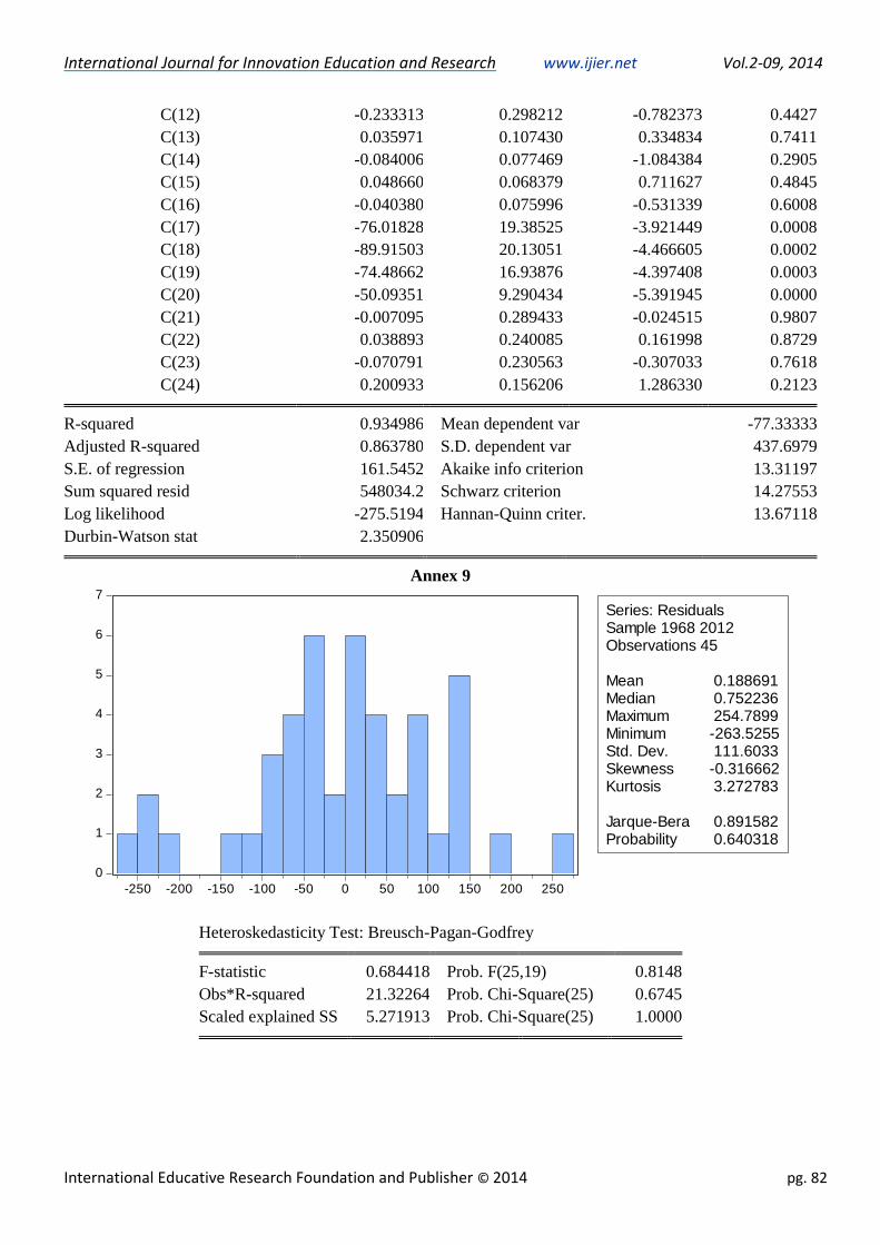
C(12) -0.233313 0.298212 -0.782373 0.4427
C(13) 0.035971 0.107430 0.334834 0.7411
C(14) -0.084006 0.077469 -1.084384 0.2905
C(15) 0.048660 0.068379 0.711627 0.4845
C(16) -0.040380 0.075996 -0.531339 0.6008
C(17) -76.01828 19.38525 -3.921449 0.0008
C(18) -89.91503 20.13051 -4.466605 0.0002
C(19) -74.48662 16.93876 -4.397408 0.0003
C(20) -50.09351 9.290434 -5.391945 0.0000
C(21) -0.007095 0.289433 -0.024515 0.9807
C(22) 0.038893 0.240085 0.161998 0.8729
C(23) -0.070791 0.230563 -0.307033 0.7618
C(24) 0.200933 0.156206 1.286330 0.2123
R-squared 0.934986 Mean dependent var -77.33333
Adjusted R-squared 0.863780 S.D. dependent var 437.6979
S.E. of regression 161.5452 Akaike info criterion 13.31197
Sum squared resid 548034.2 Schwarz criterion 14.27553
Log likelihood -275.5194 Hannan-Quinn criter. 13.67118
Durbin-Watson stat 2.350906
Annex 9
Heteroskedasticity Test: Breusch-Pagan-Godfrey
F-statistic 0.684418 Prob. F(25,19) 0.8148
Obs*R-squared 21.32264 Prob. Chi-Square(25) 0.6745
Scaled explained SS 5.271913 Prob. Chi-Square(25) 1.0000
0
1
2
3
4
5
6
7
-250 -200 -150 -100 -50 0 50 100 150 200 250
Series: ResidualsSample 1968 2012Observations 45
Mean 0.188691Median 0.752236Maximum 254.7899Minimum -263.5255Std. Dev. 111.6033Skewness -0.316662Kurtosis 3.272783
Jarque-Bera 0.891582Probability 0.640318
International Journal for Innovation Education and Research www.ijier.net Vol.2-09, 2014
International Educative Research Foundation and Publisher © 2014 pg. 83
Breusch-Godfrey Serial Correlation LM Test:
F-statistic 0.575114 Prob. F(2,19) 0.5721
Obs*R-squared 2.568596 Prob. Chi-Square(2) 0.2768
10. VAR lag order selection criteria
Sample (adjusted): 1968- 2011
Included observations: 44 after adjustments
Trend assumption: No deterministic trend (restricted constant)
Series: CAD DEF GDP INT MON
Lags interval (in first differences): 1 to 4
Unrestricted Cointegration Rank Test (Trace)
Hypothesized Trace 0.05
No. of CE(s) Eigenvalue Statistic Critical Value Max-Eigen 0.05
Statistic Critical Value Prob.**
None * 0.878353 207.9289 76.97277 92.69172 34.80587* 0.0000
At most 1 * 0.807137 115.2371 54.07904 72.41412 28.58808* 0.0000
At most 2 * 0.379253 42.82303 35.19275 20.98060 22.29962 0.0756
At most 3 * 0.264711 21.84243 20.26184 13.52961 15.89210 0.1135
At most 4 0.172154 8.312820 9.164546 8.312820 9.164546 0.0724
Trace test indicates 4 cointegrating eqn(s) at the 0.05 level
* denotes rejection of the hypothesis at the 0.05 level
**MacKinnon-Haug-Michelis (1999) p-values
Max-eigenvalue test indicates 2 cointegrating eqn(s) at the
0.05 level
Unrestricted Cointegration Rank Test (Maximum Eigenvalue)
Hypothesized Max-Eigen 0.05
No. of CE(s) Eigenvalue Statistic Critical Value Prob.**
None * 0.878353 92.69172 34.80587 0.0000
At most 1 * 0.807137 72.41412 28.58808 0.0000
At most 2 0.379253 20.98060 22.29962 0.0756
At most 3 0.264711 13.52961 15.89210 0.1135
At most 4 0.172154 8.312820 9.164546 0.0724
Max-eigenvalue test indicates 2 cointegrating eqn(s) at the 0.05 level
* denotes rejection of the hypothesis at the 0.05 level
**MacKinnon-Haug-Michelis (1999) p-values
International Journal for Innovation Education and Research www.ijier.net Vol.2-09, 2014
International Educative Research Foundation and Publisher © 2014 pg. 84
Unrestricted Cointegrating Coefficients (normalized by b'*S11*b=I):
CAD DEFICIT GDP INTEREST MONEY C
0.014462 -0.017163 -0.003501 -0.719468 0.011988 4.736024
3.01E-05 0.009282 0.002896 -0.030004 -0.006561 -1.392996
0.006962 -0.019609 -0.001009 -0.292954 0.002953 0.929213
0.007371 -0.015939 -0.000697 -0.256790 0.002894 1.238343
-0.010469 0.012588 0.000857 0.180896 -0.003264 0.238610
Unrestricted Adjustment Coefficients (alpha):
D(CAD) -127.3257 -147.7538 5.382200 4.090633 -11.28189
D(DEFICIT) -59.64641 41.28463 13.78281 8.102224 -44.08798
D(GDP) 352.4688 84.65421 -530.0570 219.5626 21.70393
D(INTEREST
) -1.296693 -0.579500 0.809794 0.749792 0.967729
D(MONEY) -381.9158 319.5844 -191.7703 -108.4241 95.21592
1 Cointegrating Equation(s): Log likelihood -1351.779
Normalized cointegrating coefficients (standard error in parentheses)
CAD DEFICIT GDP INTEREST MONEY C
1.000000 -1.186726 -0.242067 -49.74867 0.828907 327.4793
(0.08554) (0.01779) (1.51523) (0.04413) (21.7321)
11.Pairwise Granger Causality Tests
Sample: 1963 2012
Lags: 2
Null Hypothesis: Obs F-Statistic Prob.
DEFICIT does not Granger Cause CAD 48 7.08185 0.0022
CAD does not Granger Cause DEFICIT 20.6519 5.E-07
GDP does not Granger Cause CAD 48 4.40555 0.0182
CAD does not Granger Cause GDP 0.56317 0.5735
INTEREST does not Granger Cause CAD 47 1.41068 0.2553
CAD does not Granger Cause INTEREST 0.31167 0.7339
MONEY does not Granger Cause CAD 48 3.03734 0.0584
CAD does not Granger Cause MONEY 0.68659 0.5087
GDP does not Granger Cause DEFICIT 48 5.63536 0.0067
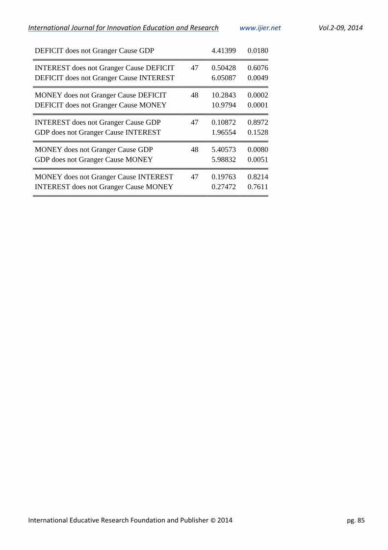
International Journal for Innovation Education and Research www.ijier.net Vol.2-09, 2014
International Educative Research Foundation and Publisher © 2014 pg. 85
DEFICIT does not Granger Cause GDP 4.41399 0.0180
INTEREST does not Granger Cause DEFICIT 47 0.50428 0.6076
DEFICIT does not Granger Cause INTEREST 6.05087 0.0049
MONEY does not Granger Cause DEFICIT 48 10.2843 0.0002
DEFICIT does not Granger Cause MONEY 10.9794 0.0001
INTEREST does not Granger Cause GDP 47 0.10872 0.8972
GDP does not Granger Cause INTEREST 1.96554 0.1528
MONEY does not Granger Cause GDP 48 5.40573 0.0080
GDP does not Granger Cause MONEY 5.98832 0.0051
MONEY does not Granger Cause INTEREST 47 0.19763 0.8214
INTEREST does not Granger Cause MONEY 0.27472 0.7611