Embed Size (px)
Citation preview
722 VOLUME 15J O U R N A L O F C L I M A T E
q 2002 American Meteorological Society
The Tropospheric Biennial Oscillation and Asian–Australian Monsoon Rainfall
GERALD A. MEEHL AND JULIE M. ARBLASTER
National Center for Atmospheric Research,* Boulder, Colorado
(Manuscript received 16 January 2001, in final form 26 September 2001)
ABSTRACT
In the context of the Asian–Australian monsoon, the tropospheric biennial oscillation (TBO) is defined as thetendency for a relatively strong monsoon to be followed by a relatively weak one, and vice versa. Thereforethe TBO is not so much an oscillation, but a tendency for the system to flip-flop back and forth from year toyear. The more of these interannual flip-flops or transitions, the more biennial the system. The transitions occurin northern spring for the south Asian or Indian monsoon and in northern fall for the Australian monsooninvolving coupled land–atmosphere–ocean processes over a large area of the Indo-Pacific region. There isconsiderable seasonal persistence from the south Asian to Australian monsoon as noted in previous studies, witha strong south Asian or Indian monsoon tending to precede a strong Australian monsoon and vice versa forweak monsoons. Therefore, transitions from March–May (MAM) to June–September (JJAS) tend to set thesystem for the next year, with a transition to the opposite sign the following year. Quantifying the role of theconditions that contribute to these transitions in the TBO and their relationship to ENSO is crucial for verifyingtheir accurate representation in models, which should lead to improved seasonal forecast skill. An analysis ofobserved data shows that the TBO (with roughly a 2–3-yr period) encompasses most ENSO years (with theirwell-known biennial tendency) as well as additional years that contribute to biennial transitions. Thus the TBOis a fundamental feature of the coupled climate system over the entire Indian–Pacific region. El Nino and LaNina events as well as Indian Ocean SST dipole events are large amplitude excursions of the TBO in the tropicalPacific and Indian Oceans, respectively, associated with coupled ocean dynamics, upper-ocean temperatureanomalies, and associated ocean heat content anomalies. Conditions postulated to contribute to TBO transitionsinvolve anomalous Asian land surface temperatures, Pacific and Indian Ocean SST anomalies, and the associatedstrength of the convective maximum over Australasia. These interannual transition conditions are quantifiedfrom singular value decomposition (SVD) analyses on a year-by-year basis using single and cumulative anomalypattern correlations. This technique takes into account intermittent influences and secular variations in the strengthof any particular association in any given year. Anomalous Pacific and Indian Ocean SSTs are the dominanttransition conditions in the TBO, with anomalous meridional temperature gradients over Asia a secondary factor.There is an intrinsic coupling of the anomalous strength of the convective maximum in the seasonal cycle overAustralasia, surface wind forcing, ocean dynamical response, and associated SST anomalies that feed back tothe strength of the convective maximum, and so on. All are tied together by the large-scale east–west circulation,the eastern and western Walker cells, in the atmosphere. By omitting El Nino and La Nina onset years fromthe analysis, there are similar but lower-amplitude relationships among the transition conditions and Asian–Australian monsoon rainfall. An SST transition in the Pacific is started by surface wind anomalies in the farwestern equatorial Pacific associated with the Australian monsoon, while an SST transition in the Indian Oceanis started by surface wind anomalies in the western equatorial Indian Ocean associated with the Indian monsoon.This provides successive forcing and response among Indian and Pacific SSTs and the Asian–Australian monsoonshalf a year apart. The consequent feedback to the monsoon circulations by the SST anomalies results in theTBO.
1. Introduction
The attribution of the strength of associations of con-ditions prior to the Asian–Australian monsoon with sub-
* The National Center for Atmospheric Research is sponsored bythe National Science Foundation.
Corresponding author address: Dr. Gerald A. Meehl, Climate andGlobal Dynamics Division, National Center for Atmospheric Re-search, P.O. Box 3000, Boulder, CO 80307.E-mail: [email protected]
sequent anomalous patterns of monsoon rainfall is oneof the fundamental human and scientific problems fac-ing the climate research community today. This is ofprimary importance to the economies of dozens of coun-tries and the livelihoods of millions of people in themonsoon regions stretching from Africa, across Asia tothe Pacific. To accurately represent coupled processesin the climate system in forecast models, we must firstidentify and quantify such processes in the observedsystem.
The tropospheric biennial oscillation (TBO) is definedhere as the tendency for a relatively strong monsoon to
1 APRIL 2002 723M E E H L A N D A R B L A S T E R
be followed by a relatively weak one, and vice versa,with the transitions occurring in the season prior to themonsoon involving coupled land–atmosphere–oceanprocesses over a large area of the Indo-Pacific region(Meehl 1997). Thus the TBO is more a tendency forthe system to flip-flop back and forth from year to year,and not so much an oscillation. The more of these in-terannual flip-flops or transitions, the more biennial thesystem.
The TBO has become recognized as a candidate forunderstanding some of the processes that can contributeto interannual variability of a variety of parameters inthe Indian and Pacific regions in both observations (Ro-pelewski et al. 1992; Yang et al. 1996; Yasunari 1990;Yasunari and Seki 1992; Tomita and Yasunari 1996;Meehl 1987, 1997; Meehl and Arblaster 2001b, here-after MEAR2) and models (Ogasawara et al. 1999;Chang and Li 2000). Though there are some alternativeexplanations concerning how the TBO can arise (e.g.,Jin et al. 1994; Goswami 1995), certain deterministicprocesses have been postulated to produce the TBO(Clarke et al. 1998; Chang and Li 2000; Meehl 1987,1993, 1994, 1997; MEAR2). One of the difficulties ofthese TBO studies has been quantifying the contributionof various proposed mechanisms. The purpose of thispaper is to address this issue, and attempt to quantifythe year-to-year contributions of conditions associatedwith TBO transitions to patterns of Asian–Australianmonsoon rainfall. We will address two questions: 1)What makes the TBO transition or ‘‘flip-flop’’ from yearto year, and 2) why is northern spring March–May(MAM) particularly important for TBO transitions?
In regards to the first question, we hypothesize thatcertain conditions in the seasons prior to the monsoon,set up by coupled interactions in the preceding year, willcause the monsoon to be relatively stronger (or weaker)than the previous or following years, thus introducinga biennial component in spectra of area-averaged mon-soon rainfall. These conditions include anomalous SSTsin the Indian and Pacific Oceans for both the south Asianand Australian monsoons, in addition to anomalous me-ridional temperature gradients over Asia prior to theIndian monsoon, and anomalous strength of the con-vective maximum prior to the Australian monsoon.
With respect to the second question, we hypothesizethat the strength of the Australian monsoon, itself setup by conditions from the previous year, producesanomalous wind forcing in the western equatorial Pa-cific. This in turn results in an ocean dynamical responsethat causes tropical Pacific SST anomalies to changesign or transition, which then can affect the subsequentIndian monsoon via the large-scale east–west atmo-spheric circulation. More details in regards to these hy-potheses will be provided below (e.g., in the discussionof Fig. 3).
Though there are a number of different types ofENSO events with protracted episodes that would weak-en biennial signals (Allan and D’Arrigo 1999; Reason
et al. 2000), enough ENSO events have inherent biennialtendencies so that a well-known biennial signature, withopposite sign precipitation and temperature anomaliesthe previous and following years, shows up in compositeEl Nino and La Nina events over a wide domain cov-ering the tropical Indian and Pacific regions (e.g., Ki-ladis and van Loon 1988; Kiladis and Diaz 1989).Therefore, the TBO clearly must encompass this bien-nial tendency of ENSO. However, it has been shownthat other years display similar patterns to ENSO in thislarge region (Meehl 1987; Lau and Wu 2001). In fact,TBO and ENSO signal strength is closer in magnitudeover the Indian Ocean than the equatorial Pacific (Rea-son et al. 2000). Therefore the TBO must include mostENSO (El Nino and La Nina) years and some otheryears as well. Yet it has been difficult to quantify thevarious processes and conditions associated with thisbiennial tendency of monsoon–ENSO interaction andthe additional non-ENSO years that contribute to theTBO (Webster et al. 1998). It has been argued that, ofthe wide array of conditions that could contribute tomonsoon transitions in the TBO, most ultimately relateto anomalous surface temperature over south Asia andthe tropical Indian and Pacific Oceans (Meehl 1997). Itis the purpose of this paper to quantify the contributionsfrom such anomalous surface conditions involved witha transition from relatively weak (strong) to relativelystrong (weak) monsoon in consecutive years that con-tribute to the TBO.
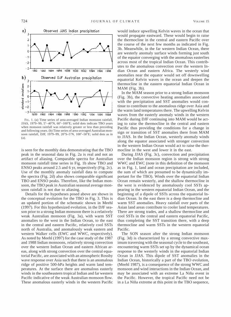
To illustrate how a biennial tendency can arise in thetime series of the annually recurring Asian–Australianmonsoons, we show time series of area-averaged pre-cipitation for the Indian monsoon (JJAS, 1979–99, 58–408N, 608–1008E, Fig. 1a) and the Australian monsoon(DJF, 1979–99, 208S–58N, 1008–1508E, Fig. 1b). Soliddots indicate monsoon rainfall relatively greater (or less)than the preceding or following years. That is, if Pi isthe value of area-averaged monsoon season precipitationfor a given year i, then a relatively strong monsoon isdefined as
P , P . Pi21 i i11
and a relatively weak monsoon is defined as
P . P , P .i21 i i11
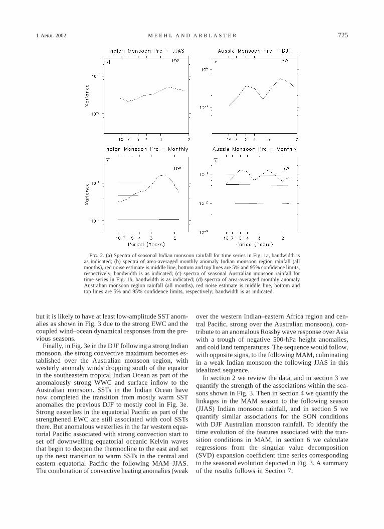
For the Indian monsoon, 13 out of 21 yr are ‘‘bien-nial’’ defined in that way, and 11 out of 21 yr for theAustralian monsoon. El Nino and La Nina onset yearscorrespond to some of those TBO years but not all. Thiswas first noted by Meehl (1987). The spectra of the timeseries in Fig. 1a shows a peak in the TBO period of 2.6yr with little ENSO peak for this time period in Fig. 2a(the relative power of ENSO and TBO vary over time,e.g., Webster et al. 1998). Since there is the possibilityof aliasing with the annual data (Madden and Jones2001), spectra of the monthly anomalies (including all12 months each year) for the Indian monsoon regionare shown in Fig. 2b. A similar significant TBO peak
724 VOLUME 15J O U R N A L O F C L I M A T E
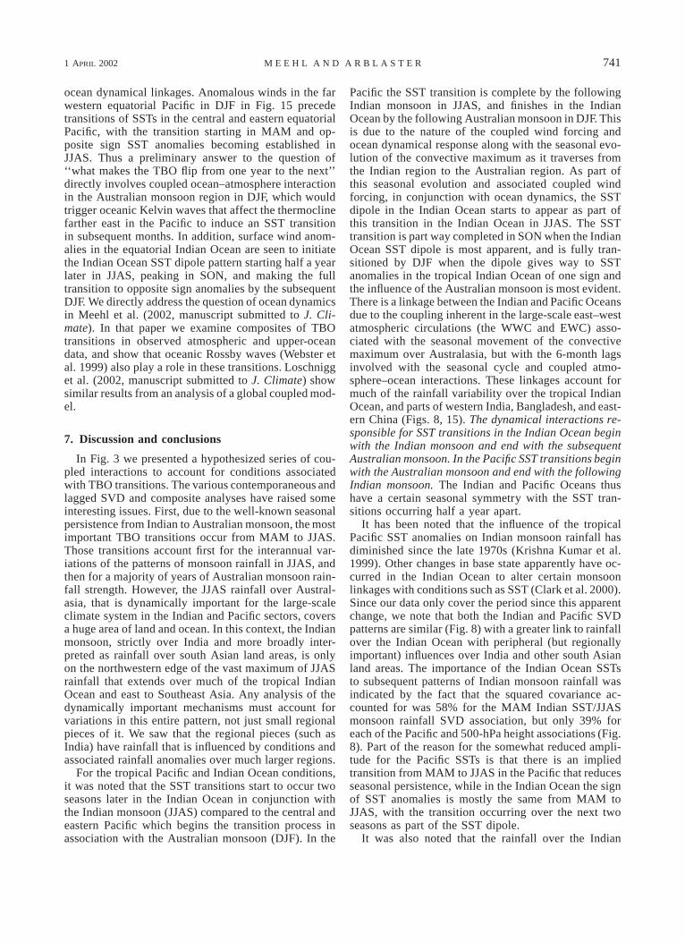
FIG. 1. (a) Time series of area-averaged Indian monsoon rainfall,JJAS, 1979–99, 58–408N, 608–1008E; solid dots indicate TBO yearswhen monsoon rainfall was relatively greater or less than precedingand following years. (b) Time series of area-averaged Australian mon-soon rainfall, DJF, 1979–99, 208S–58N, 1008–508E; solid dots as in(a).
is seen for the monthly data demonstrating that the TBOpeak in the seasonal data in Fig. 2a is real and not anartifact of aliasing. Comparable spectra for Australianmonsoon rainfall time series in Fig. 1b show TBO andENSO peaks around 2.5 and 6 yr, respectively (Fig. 2c).Use of the monthly anomaly rainfall data to computethe spectra (Fig. 2d) also shows comparable significantTBO and ENSO peaks. Therefore, like the Indian mon-soon, the TBO peak in Australian seasonal average mon-soon rainfall is not due to aliasing.
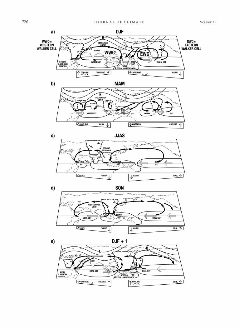
Details for the hypotheses posed above are shown inthe conceptual evolution for the TBO in Fig. 3. This isan updated portion of the schematic shown in Meehl(1997). For this hypothesized evolution, in the DJF sea-son prior to a strong Indian monsoon there is a relativelyweak Australian monsoon (Fig. 3a), with warm SSTanomalies to the west in the Indian Ocean, to the eastin the central and eastern Pacific, relatively cool SSTsnorth of Australia, and anomalously weak eastern andwestern Walker cells (EWC and WWC, respectively).As noted by Meehl (1997) for the case study of the 1987and 1988 Indian monsoons, relatively strong convectionover the western Indian Ocean and eastern African ar-eas, along with strong convection over the central equa-torial Pacific, are associated with an atmospheric Rossbywave response over Asia such that there is an anomalousridge of positive 500-hPa heights and warm land tem-peratures. At the surface there are anomalous easterlywinds in the southeastern tropical Indian and far westernPacific indicative of the weak Australian monsoon flow.These anomalous easterly winds in the western Pacific
would induce upwelling Kelvin waves in the ocean thatwould propagate eastward. These would begin to raisethe thermocline in the central and eastern Pacific overthe course of the next few months as indicated in Fig.3b. Meanwhile, in the far western Indian Ocean, thereare westerly anomaly surface winds forming just southof the equator converging with the anomalous easterliesacross most of the tropical Indian Ocean. This contrib-utes to the anomalous convection over the western In-dian Ocean and eastern Africa. The westerly windanomalies near the equator would set off downwellingequatorial Kelvin waves in the ocean and deepen thethermocline in the eastern equatorial Indian Ocean inMAM (Fig. 3b).
In the MAM season prior to a strong Indian monsoon(Fig. 3b), the convective heating anomalies associatedwith the precipitation and SST anomalies would con-tinue to contribute to the anomalous ridge over Asia andthe warm land temperatures there. The upwelling Kelvinwaves from the easterly anomaly winds in the westernPacific during DJF continuing into MAM would be act-ing to raise the thermocline in the central and easternPacific thus providing the conditions for a change insign or transition of SST anomalies there from MAMto JJAS. In the Indian Ocean, westerly anomaly windsalong the equator associated with stronger convectionin the western Indian Ocean would act to raise the ther-mocline in the west and lower it in the east.
During JJAS (Fig. 3c), convection and precipitationover the Indian monsoon region is strong with strongWWC and EWC (note in this definition of the monsoonas in Fig. 1, land and ocean precipitation are included,the sum of which are presumed to be dynamically im-portant for the TBO). Winds over the equatorial IndianOcean remain westerly, and the shallow thermocline inthe west is evidenced by anomalously cool SSTs ap-pearing in the western equatorial Indian Ocean, and thebeginning of a dipole of SSTs across the equatorial In-dian Ocean. In the east there is a deep thermocline andwarm SST anomalies. Heavy rainfall over parts of theAsian land areas contribute to cooler land temperatures.There are strong trades, and a shallow thermocline andcool SSTs in the central and eastern equatorial Pacific,thus completing the SST transition there, with a deepthermocline and warm SSTs in the western equatorialPacific.
The SON season after the strong Indian monsoon(Fig. 3d) is characterized by a strong convective max-imum traversing with the seasonal cycle to the southeast,encountering warm SSTs set up by the dynamical oceanresponse to the westerly winds in the equatorial IndianOcean in JJAS. This dipole of SST anomalies in theIndian Ocean, historically a part of the TBO evolution,(Meehl 1987), is a consequence of the strong WWC andmonsoon and wind interactions in the Indian Ocean, andmay be associated with an extreme La Nina event inthe Pacific. However, the tropical Pacific need not bein a La Nina extreme at this point in the TBO sequence,
1 APRIL 2002 725M E E H L A N D A R B L A S T E R
FIG. 2. (a) Spectra of seasonal Indian monsoon rainfall for time series in Fig. 1a, bandwidth isas indicated; (b) spectra of area-averaged monthly anomaly Indian monsoon region rainfall (allmonths), red noise estimate is middle line, bottom and top lines are 5% and 95% confidence limits,respectively, bandwidth is as indicated; (c) spectra of seasonal Australian monsoon rainfall fortime series in Fig. 1b, bandwidth is as indicated; (d) spectra of area-averaged monthly anomalyAustralian monsoon region rainfall (all months), red noise estimate is middle line, bottom andtop lines are 5% and 95% confidence limits, respectively; bandwidth is as indicated.
but it is likely to have at least low-amplitude SST anom-alies as shown in Fig. 3 due to the strong EWC and thecoupled wind–ocean dynamical responses from the pre-vious seasons.
Finally, in Fig. 3e in the DJF following a strong Indianmonsoon, the strong convective maximum becomes es-tablished over the Australian monsoon region, withwesterly anomaly winds dropping south of the equatorin the southeastern tropical Indian Ocean as part of theanomalously strong WWC and surface inflow to theAustralian monsoon. SSTs in the Indian Ocean havenow completed the transition from mostly warm SSTanomalies the previous DJF to mostly cool in Fig. 3e.Strong easterlies in the equatorial Pacific as part of thestrengthened EWC are still associated with cool SSTsthere. But anomalous westerlies in the far western equa-torial Pacific associated with strong convection start toset off downwelling equatorial oceanic Kelvin wavesthat begin to deepen the thermocline to the east and setup the next transition to warm SSTs in the central andeastern equatorial Pacific the following MAM–JJAS.The combination of convective heating anomalies (weak
over the western Indian–eastern Africa region and cen-tral Pacific, strong over the Australian monsoon), con-tribute to an anomalous Rossby wave response over Asiawith a trough of negative 500-hPa height anomalies,and cold land temperatures. The sequence would follow,with opposite signs, to the following MAM, culminatingin a weak Indian monsoon the following JJAS in thisidealized sequence.
In section 2 we review the data, and in section 3 wequantify the strength of the associations within the sea-sons shown in Fig. 3. Then in section 4 we quantify thelinkages in the MAM season to the following season(JJAS) Indian monsoon rainfall, and in section 5 wequantify similar associations for the SON conditionswith DJF Australian monsoon rainfall. To identify thetime evolution of the features associated with the tran-sition conditions in MAM, in section 6 we calculateregressions from the singular value decomposition(SVD) expansion coefficient time series correspondingto the seasonal evolution depicted in Fig. 3. A summaryof the results follows in Section 7.
726 VOLUME 15J O U R N A L O F C L I M A T E
1 APRIL 2002 727M E E H L A N D A R B L A S T E R
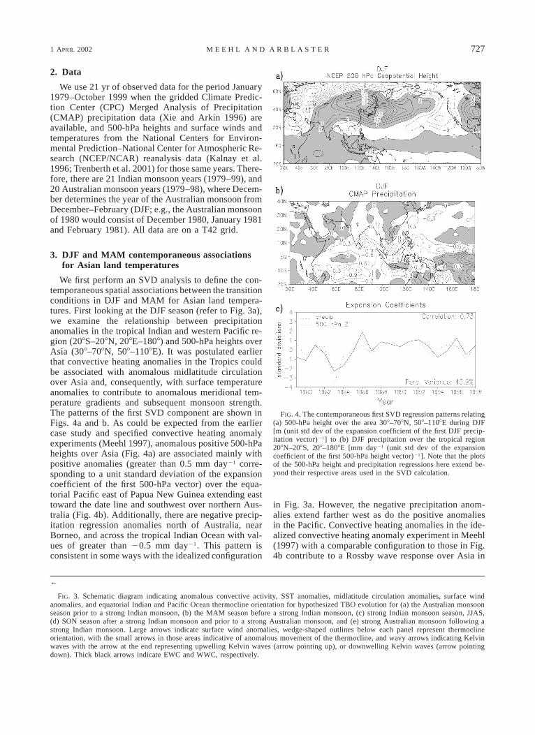
FIG. 4. The contemporaneous first SVD regression patterns relating(a) 500-hPa height over the area 308–708N, 508–1108E during DJF[m (unit std dev of the expansion coefficient of the first DJF precip-itation vector)21] to (b) DJF precipitation over the tropical region208N–208S, 208–1808E [mm day21 (unit std dev of the expansioncoefficient of the first 500-hPa height vector)21]. Note that the plotsof the 500-hPa height and precipitation regressions here extend be-yond their respective areas used in the SVD calculation.
←
FIG. 3. Schematic diagram indicating anomalous convective activity, SST anomalies, midlatitude circulation anomalies, surface windanomalies, and equatorial Indian and Pacific Ocean thermocline orientation for hypothesized TBO evolution for (a) the Australian monsoonseason prior to a strong Indian monsoon, (b) the MAM season before a strong Indian monsoon, (c) strong Indian monsoon season, JJAS,(d) SON season after a strong Indian monsoon and prior to a strong Australian monsoon, and (e) strong Australian monsoon following astrong Indian monsoon. Large arrows indicate surface wind anomalies, wedge-shaped outlines below each panel represent thermoclineorientation, with the small arrows in those areas indicative of anomalous movement of the thermocline, and wavy arrows indicating Kelvinwaves with the arrow at the end representing upwelling Kelvin waves (arrow pointing up), or downwelling Kelvin waves (arrow pointingdown). Thick black arrows indicate EWC and WWC, respectively.
2. Data
We use 21 yr of observed data for the period January1979–October 1999 when the gridded Climate Predic-tion Center (CPC) Merged Analysis of Precipitation(CMAP) precipitation data (Xie and Arkin 1996) areavailable, and 500-hPa heights and surface winds andtemperatures from the National Centers for Environ-mental Prediction–National Center for Atmospheric Re-search (NCEP/NCAR) reanalysis data (Kalnay et al.1996; Trenberth et al. 2001) for those same years. There-fore, there are 21 Indian monsoon years (1979–99), and20 Australian monsoon years (1979–98), where Decem-ber determines the year of the Australian monsoon fromDecember–February (DJF; e.g., the Australian monsoonof 1980 would consist of December 1980, January 1981and February 1981). All data are on a T42 grid.
3. DJF and MAM contemporaneous associationsfor Asian land temperatures
We first perform an SVD analysis to define the con-temporaneous spatial associations between the transitionconditions in DJF and MAM for Asian land tempera-tures. First looking at the DJF season (refer to Fig. 3a),we examine the relationship between precipitationanomalies in the tropical Indian and western Pacific re-gion (208S–208N, 208E–1808) and 500-hPa heights overAsia (308–708N, 508–1108E). It was postulated earlierthat convective heating anomalies in the Tropics couldbe associated with anomalous midlatitude circulationover Asia and, consequently, with surface temperatureanomalies to contribute to anomalous meridional tem-perature gradients and subsequent monsoon strength.The patterns of the first SVD component are shown inFigs. 4a and b. As could be expected from the earliercase study and specified convective heating anomalyexperiments (Meehl 1997), anomalous positive 500-hPaheights over Asia (Fig. 4a) are associated mainly withpositive anomalies (greater than 0.5 mm day21 corre-sponding to a unit standard deviation of the expansioncoefficient of the first 500-hPa vector) over the equa-torial Pacific east of Papua New Guinea extending easttoward the date line and southwest over northern Aus-tralia (Fig. 4b). Additionally, there are negative precip-itation regression anomalies north of Australia, nearBorneo, and across the tropical Indian Ocean with val-ues of greater than 20.5 mm day21. This pattern isconsistent in some ways with the idealized configuration
in Fig. 3a. However, the negative precipitation anom-alies extend farther west as do the positive anomaliesin the Pacific. Convective heating anomalies in the ide-alized convective heating anomaly experiment in Meehl(1997) with a comparable configuration to those in Fig.4b contribute to a Rossby wave response over Asia in
728 VOLUME 15J O U R N A L O F C L I M A T E
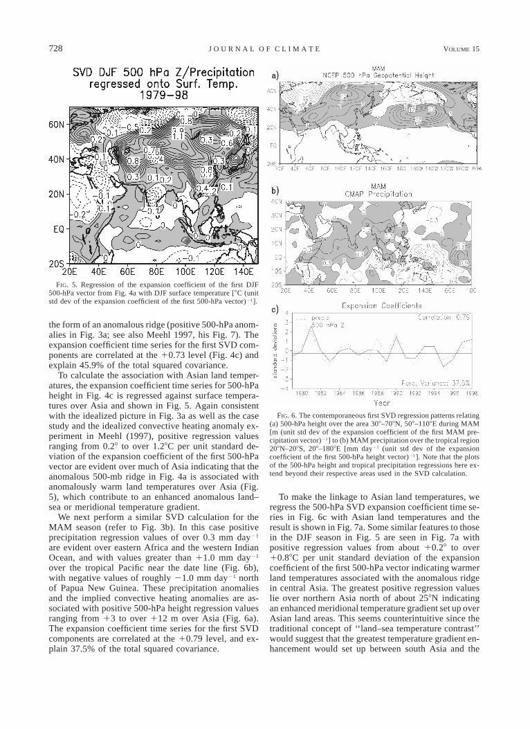
FIG. 5. Regression of the expansion coefficient of the first DJF500-hPa vector from Fig. 4a with DJF surface temperature [8C (unitstd dev of the expansion coefficient of the first 500-hPa vector)21].
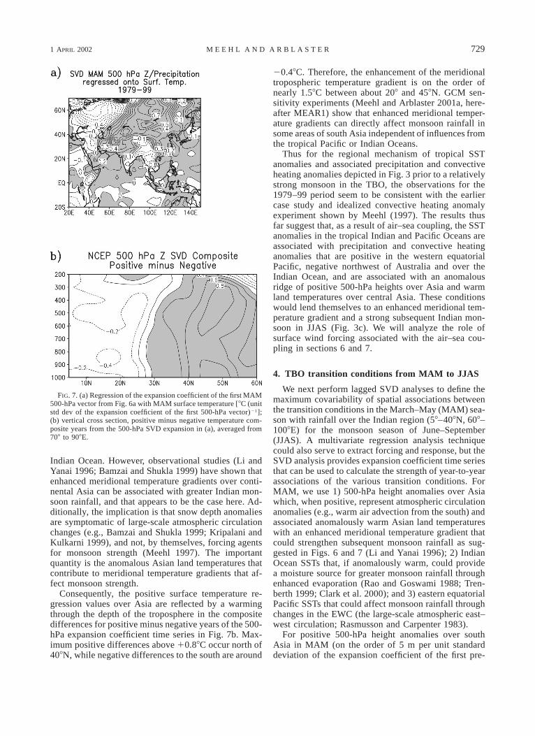
FIG. 6. The contemporaneous first SVD regression patterns relating(a) 500-hPa height over the area 308–708N, 508–1108E during MAM[m (unit std dev of the expansion coefficient of the first MAM pre-cipitation vector)21] to (b) MAM precipitation over the tropical region208N–208S, 208–1808E [mm day21 (unit std dev of the expansioncoefficient of the first 500-hPa height vector)21]. Note that the plotsof the 500-hPa height and tropical precipitation regressions here ex-tend beyond their respective areas used in the SVD calculation.
the form of an anomalous ridge (positive 500-hPa anom-alies in Fig. 3a; see also Meehl 1997, his Fig. 7). Theexpansion coefficient time series for the first SVD com-ponents are correlated at the 10.73 level (Fig. 4c) andexplain 45.9% of the total squared covariance.
To calculate the association with Asian land temper-atures, the expansion coefficient time series for 500-hPaheight in Fig. 4c is regressed against surface tempera-tures over Asia and shown in Fig. 5. Again consistentwith the idealized picture in Fig. 3a as well as the casestudy and the idealized convective heating anomaly ex-periment in Meehl (1997), positive regression valuesranging from 0.28 to over 1.28C per unit standard de-viation of the expansion coefficient of the first 500-hPavector are evident over much of Asia indicating that theanomalous 500-mb ridge in Fig. 4a is associated withanomalously warm land temperatures over Asia (Fig.5), which contribute to an enhanced anomalous land–sea or meridional temperature gradient.
We next perform a similar SVD calculation for theMAM season (refer to Fig. 3b). In this case positiveprecipitation regression values of over 0.3 mm day21
are evident over eastern Africa and the western IndianOcean, and with values greater than 11.0 mm day21
over the tropical Pacific near the date line (Fig. 6b),with negative values of roughly 21.0 mm day21 northof Papua New Guinea. These precipitation anomaliesand the implied convective heating anomalies are as-sociated with positive 500-hPa height regression valuesranging from 13 to over 112 m over Asia (Fig. 6a).The expansion coefficient time series for the first SVDcomponents are correlated at the 10.79 level, and ex-plain 37.5% of the total squared covariance.
To make the linkage to Asian land temperatures, weregress the 500-hPa SVD expansion coefficient time se-ries in Fig. 6c with Asian land temperatures and theresult is shown in Fig. 7a. Some similar features to thosein the DJF season in Fig. 5 are seen in Fig. 7a withpositive regression values from about 10.28 to over10.88C per unit standard deviation of the expansioncoefficient of the first 500-hPa vector indicating warmerland temperatures associated with the anomalous ridgein central Asia. The greatest positive regression valueslie over northern Asia north of about 258N indicatingan enhanced meridional temperature gradient set up overAsian land areas. This seems counterintuitive since thetraditional concept of ‘‘land–sea temperature contrast’’would suggest that the greatest temperature gradient en-hancement would set up between south Asia and the
1 APRIL 2002 729M E E H L A N D A R B L A S T E R
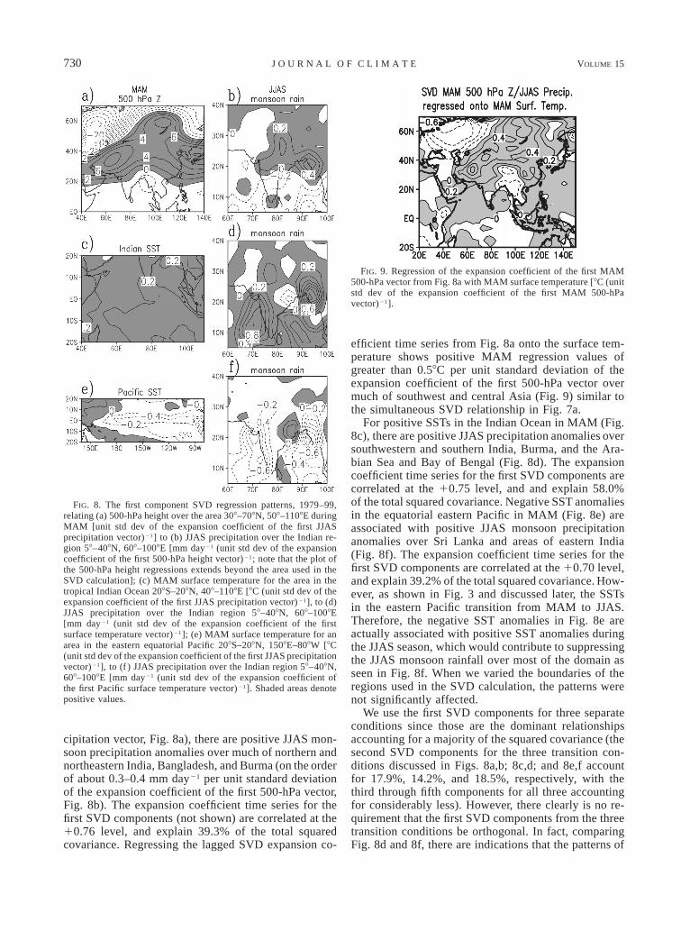
FIG. 7. (a) Regression of the expansion coefficient of the first MAM500-hPa vector from Fig. 6a with MAM surface temperature [8C (unitstd dev of the expansion coefficient of the first 500-hPa vector)21];(b) vertical cross section, positive minus negative temperature com-posite years from the 500-hPa SVD expansion in (a), averaged from708 to 908E.
Indian Ocean. However, observational studies (Li andYanai 1996; Bamzai and Shukla 1999) have shown thatenhanced meridional temperature gradients over conti-nental Asia can be associated with greater Indian mon-soon rainfall, and that appears to be the case here. Ad-ditionally, the implication is that snow depth anomaliesare symptomatic of large-scale atmospheric circulationchanges (e.g., Bamzai and Shukla 1999; Kripalani andKulkarni 1999), and not, by themselves, forcing agentsfor monsoon strength (Meehl 1997). The importantquantity is the anomalous Asian land temperatures thatcontribute to meridional temperature gradients that af-fect monsoon strength.
Consequently, the positive surface temperature re-gression values over Asia are reflected by a warmingthrough the depth of the troposphere in the compositedifferences for positive minus negative years of the 500-hPa expansion coefficient time series in Fig. 7b. Max-imum positive differences above 10.88C occur north of408N, while negative differences to the south are around
20.48C. Therefore, the enhancement of the meridionaltropospheric temperature gradient is on the order ofnearly 1.58C between about 208 and 458N. GCM sen-sitivity experiments (Meehl and Arblaster 2001a, here-after MEAR1) show that enhanced meridional temper-ature gradients can directly affect monsoon rainfall insome areas of south Asia independent of influences fromthe tropical Pacific or Indian Oceans.
Thus for the regional mechanism of tropical SSTanomalies and associated precipitation and convectiveheating anomalies depicted in Fig. 3 prior to a relativelystrong monsoon in the TBO, the observations for the1979–99 period seem to be consistent with the earliercase study and idealized convective heating anomalyexperiment shown by Meehl (1997). The results thusfar suggest that, as a result of air–sea coupling, the SSTanomalies in the tropical Indian and Pacific Oceans areassociated with precipitation and convective heatinganomalies that are positive in the western equatorialPacific, negative northwest of Australia and over theIndian Ocean, and are associated with an anomalousridge of positive 500-hPa heights over Asia and warmland temperatures over central Asia. These conditionswould lend themselves to an enhanced meridional tem-perature gradient and a strong subsequent Indian mon-soon in JJAS (Fig. 3c). We will analyze the role ofsurface wind forcing associated with the air–sea cou-pling in sections 6 and 7.
4. TBO transition conditions from MAM to JJAS
We next perform lagged SVD analyses to define themaximum covariability of spatial associations betweenthe transition conditions in the March–May (MAM) sea-son with rainfall over the Indian region (58–408N, 608–1008E) for the monsoon season of June–September(JJAS). A multivariate regression analysis techniquecould also serve to extract forcing and response, but theSVD analysis provides expansion coefficient time seriesthat can be used to calculate the strength of year-to-yearassociations of the various transition conditions. ForMAM, we use 1) 500-hPa height anomalies over Asiawhich, when positive, represent atmospheric circulationanomalies (e.g., warm air advection from the south) andassociated anomalously warm Asian land temperatureswith an enhanced meridional temperature gradient thatcould strengthen subsequent monsoon rainfall as sug-gested in Figs. 6 and 7 (Li and Yanai 1996); 2) IndianOcean SSTs that, if anomalously warm, could providea moisture source for greater monsoon rainfall throughenhanced evaporation (Rao and Goswami 1988; Tren-berth 1999; Clark et al. 2000); and 3) eastern equatorialPacific SSTs that could affect monsoon rainfall throughchanges in the EWC (the large-scale atmospheric east–west circulation; Rasmusson and Carpenter 1983).
For positive 500-hPa height anomalies over southAsia in MAM (on the order of 5 m per unit standarddeviation of the expansion coefficient of the first pre-
730 VOLUME 15J O U R N A L O F C L I M A T E
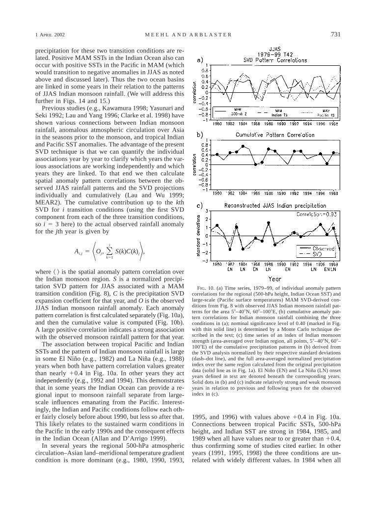
FIG. 8. The first component SVD regression patterns, 1979–99,relating (a) 500-hPa height over the area 308–708N, 508–1108E duringMAM [unit std dev of the expansion coefficient of the first JJASprecipitation vector)21] to (b) JJAS precipitation over the Indian re-gion 58–408N, 608–1008E [mm day21 (unit std dev of the expansioncoefficient of the first 500-hPa height vector)21; note that the plot ofthe 500-hPa height regressions extends beyond the area used in theSVD calculation]; (c) MAM surface temperature for the area in thetropical Indian Ocean 208S–208N, 408–1108E [8C (unit std dev of theexpansion coefficient of the first JJAS precipitation vector)21], to (d)JJAS precipitation over the Indian region 58–408N, 608–1008E[mm day21 (unit std dev of the expansion coefficient of the firstsurface temperature vector)21]; (e) MAM surface temperature for anarea in the eastern equatorial Pacific 208S–208N, 1508E–808W [8C(unit std dev of the expansion coefficient of the first JJAS precipitationvector)21], to (f ) JJAS precipitation over the Indian region 58–408N,608–1008E [mm day21 (unit std dev of the expansion coefficient ofthe first Pacific surface temperature vector)21]. Shaded areas denotepositive values.
FIG. 9. Regression of the expansion coefficient of the first MAM500-hPa vector from Fig. 8a with MAM surface temperature [8C (unitstd dev of the expansion coefficient of the first MAM 500-hPavector)21].
cipitation vector, Fig. 8a), there are positive JJAS mon-soon precipitation anomalies over much of northern andnortheastern India, Bangladesh, and Burma (on the orderof about 0.3–0.4 mm day21 per unit standard deviationof the expansion coefficient of the first 500-hPa vector,Fig. 8b). The expansion coefficient time series for thefirst SVD components (not shown) are correlated at the10.76 level, and explain 39.3% of the total squaredcovariance. Regressing the lagged SVD expansion co-
efficient time series from Fig. 8a onto the surface tem-perature shows positive MAM regression values ofgreater than 0.58C per unit standard deviation of theexpansion coefficient of the first 500-hPa vector overmuch of southwest and central Asia (Fig. 9) similar tothe simultaneous SVD relationship in Fig. 7a.
For positive SSTs in the Indian Ocean in MAM (Fig.8c), there are positive JJAS precipitation anomalies oversouthwestern and southern India, Burma, and the Ara-bian Sea and Bay of Bengal (Fig. 8d). The expansioncoefficient time series for the first SVD components arecorrelated at the 10.75 level, and and explain 58.0%of the total squared covariance. Negative SST anomaliesin the equatorial eastern Pacific in MAM (Fig. 8e) areassociated with positive JJAS monsoon precipitationanomalies over Sri Lanka and areas of eastern India(Fig. 8f). The expansion coefficient time series for thefirst SVD components are correlated at the 10.70 level,and explain 39.2% of the total squared covariance. How-ever, as shown in Fig. 3 and discussed later, the SSTsin the eastern Pacific transition from MAM to JJAS.Therefore, the negative SST anomalies in Fig. 8e areactually associated with positive SST anomalies duringthe JJAS season, which would contribute to suppressingthe JJAS monsoon rainfall over most of the domain asseen in Fig. 8f. When we varied the boundaries of theregions used in the SVD calculation, the patterns werenot significantly affected.
We use the first SVD components for three separateconditions since those are the dominant relationshipsaccounting for a majority of the squared covariance (thesecond SVD components for the three transition con-ditions discussed in Figs. 8a,b; 8c,d; and 8e,f accountfor 17.9%, 14.2%, and 18.5%, respectively, with thethird through fifth components for all three accountingfor considerably less). However, there clearly is no re-quirement that the first SVD components from the threetransition conditions be orthogonal. In fact, comparingFig. 8d and 8f, there are indications that the patterns of
1 APRIL 2002 731M E E H L A N D A R B L A S T E R
FIG. 10. (a) Time series, 1979–99, of individual anomaly patterncorrelations for the regional (500-hPa height, Indian Ocean SST) andlarge-scale (Pacific surface temperatures) MAM SVD-derived con-ditions from Fig. 8 with observed JJAS Indian monsoon rainfall pat-terns for the area 58–408N, 608–1008E, (b) cumulative anomaly pat-tern correlations for Indian monsoon rainfall combining the threeconditions in (a); nominal significance level of 0.40 (marked in Fig.with thin solid line) is determined by a Monte Carlo technique de-scribed in the text; (c) time series of an index of Indian monsoonstrength (area-averaged over Indian region, all points, 58–408N, 608–1008E) of the cumulative precipitation patterns in (b) derived fromthe SVD analysis normalized by their respective standard deviations(dash–dot line), and the full area-averaged normalized precipitationindex over the same region calculated from the original precipitationdata (solid line as in Fig. 1a). El Nino (EN) and La Nina (LN) onsetyears defined in text are denoted beneath the corresponding years.Solid dots in (b) and (c) indicate relatively strong and weak monsoonyears in relation to previous and following years for the observedindex in (c).
precipitation for these two transition conditions are re-lated. Positive MAM SSTs in the Indian Ocean also canoccur with positive SSTs in the Pacific in MAM (whichwould transition to negative anomalies in JJAS as notedabove and discussed later). Thus the two ocean basinsare linked in some years in their relation to the patternsof JJAS Indian monsoon rainfall. (We will address thisfurther in Figs. 14 and 15.)
Previous studies (e.g., Kawamura 1998; Yasunari andSeki 1992; Lau and Yang 1996; Clarke et al. 1998) haveshown various connections between Indian monsoonrainfall, anomalous atmospheric circulation over Asiain the seasons prior to the monsoon, and tropical Indianand Pacific SST anomalies. The advantage of the presentSVD technique is that we can quantify the individualassociations year by year to clarify which years the var-ious associations are working independently and whichyears they are linked. To that end we then calculatespatial anomaly pattern correlations between the ob-served JJAS rainfall patterns and the SVD projectionsindividually and cumulatively (Lau and Wu 1999;MEAR2). The cumulative contribution up to the kthSVD for i transition conditions (using the first SVDcomponent from each of the three transition conditions,so i 5 3 here) to the actual observed rainfall anomalyfor the jth year is given by
i
A 5 O , S(k)C(k) ,Oi, j j j7 8k51
where ^ & is the spatial anomaly pattern correlation overthe Indian monsoon region. S is a normalized precipi-tation SVD pattern for JJAS associated with a MAMtransition condition (Fig. 8), C is the precipitation SVDexpansion coefficient for that year, and O is the observedJJAS Indian monsoon rainfall anomaly. Each anomalypattern correlation is first calculated separately (Fig. 10a),and then the cumulative value is computed (Fig. 10b).A large positive correlation indicates a strong associationwith the observed monsoon rainfall pattern for that year.
The association between tropical Pacific and IndianSSTs and the pattern of Indian monsoon rainfall is largein some El Nino (e.g., 1982) and La Nina (e.g., 1988)years when both have pattern correlation values greaterthan nearly 10.4 in Fig. 10a. In other years they actindependently (e.g., 1992 and 1994). This demonstratesthat in some years the Indian Ocean can provide a re-gional input to monsoon rainfall separate from large-scale influences emanating from the Pacific. Interest-ingly, the Indian and Pacific conditions follow each oth-er fairly closely before about 1990, but less so after that.This likely relates to the sustained warm conditions inthe Pacific in the early 1990s and the consequent effectsin the Indian Ocean (Allan and D’Arrigo 1999).
In several years the regional 500-hPa atmosphericcirculation–Asian land–meridional temperature gradientcondition is more dominant (e.g., 1980, 1990, 1993,
1995, and 1996) with values above 10.4 in Fig. 10a.Connections between tropical Pacific SSTs, 500-hPaheight, and Indian SST are strong in 1984, 1985, and1989 when all have values near to or greater than 10.4,thus confirming some of studies cited earlier. In otheryears (1991, 1995, 1998) the three conditions are un-related with widely different values. In 1984 when all
732 VOLUME 15J O U R N A L O F C L I M A T E
three transition conditions have high values (Fig. 10a),the cumulative value is about 10.8 (Fig. 10b) indicatingover 60% of the spatial variance of the pattern of mon-soon precipitation is accounted for in that year. Howeverin 1986 when all of the three conditions are near zerofor their individual associations, the cumulative patterncorrelation is also near zero indicating other processesor internal dynamics are more important for the patternof monsoon rainfall in that year. The point is that inany given year, we quantify the magnitude of the as-sociations of the various transition conditions (eithernone, some, or all) in MAM with the subsequent JJASmonsoon rainfall.
A nominal significance level of 0.4 in Fig. 10b isdetermined by a Monte Carlo technique whereby theseasonal pattern correlations from the SVD componentsare scrambled to randomly generate 865 sample patterncorrelations with no overlap with the actual cumulativepattern correlations in Fig. 10b. A Student’s t-test isperformed to determine that the mean value of 0.4 issignificantly different from the mean of the random sam-ples (using 884 degrees of freedom) at greater than the1% level. For the 21 yr considered here from 1979 to1999, 12 (57%) exceed this nominal significance level.
To relate the precipitation anomaly patterns to anarea-averaged monsoon index and consequently themagnitude of the TBO, regressions of the SVD expan-sion coefficient time series and the SVD rainfall patternsover the Indian region are used to produce a cumulativearea-averaged Indian rainfall index (Fig. 10c). The cor-relation between the SVD-derived normalized cumu-lative index of monsoon ‘‘strength’’ and the full area-averaged normalized index from the original CMAPprecipitation data is 10.93 (significant at greater thanthe 1% level) thus showing the SVD-derived index cancapture 86% of the variance of the full index. Therefore,in Fig. 10 we quantify individual contributions to thepattern of monsoon rainfall from several transition con-ditions (Fig. 10a), the cumulative contributions to thepattern of monsoon rainfall (Fig. 10b), and a recon-structed area-averaged index of strength of the monsoon(Fig. 10c).
As noted earlier in relation to Fig. 1, TBO monsoonyears can be defined as a monsoon index value greaterthan the previous or following year, or less than theprevious or following year (Meehl 1987). These aredenoted in Fig. 10c (as in Fig. 1a) for 13 yr (out of 21yr total). We define onset years for El Nino (1982, 1986,1991, 1997) and La Nina (1984, 1988, 1995, 1998) asthe initiation of a 5-month running mean area-averagedSST anomaly in the eastern tropical Pacific Nino-3 area(58N–58S, 1508–908W) of at least 60.58C for two con-secutive seasons after the MAM transition season overthe following 1-yr period. Of the TBO years, 1982,1986, 1997 are El Nino onset years, and 1984, 1988,and 1998 are La Nina onset years for a total of 6 TBOyears out of 8 possible ENSO onset years. That leaves1980, 1983, 1987, 1989, 1992, 1993, and 1996 as 7
non-ENSO onset years that also are contributing to theinterannual flip-flops that characterize the TBO in mon-soon rainfall. In Fig. 10b, 10 of these 13 TBO yearshave greater than the nominal significance value of 0.4,indicating that the transition conditions in Fig. 8 arestrongly associated with 77% of the years with TBOtransitions.
Another way of quantifying the TBO is to first com-pute spectra of area-averaged time series of SVD-re-constructed JJAS monsoon rainfall as in Fig. 10c foreach condition in Fig. 10a individually and then cu-mulatively, and then average the power in the TBO bandof 2.1–2.8 yr. The TBO spectral density [(mm2 day22 yr)3 1021] for the individual 500-hPa SVD is 0.1. Addingthe contribution of the Pacific SST conditions increasesthe TBO amplitude to 2.2. Including the effects fromthe Indian Ocean SST conditions, such that all threetransition conditions are accounted for, increases TBOamplitude to 8.3, which is 8% greater than the spectraldensity in the ENSO periods of 3–7 yr derived in thesame way. This increase in TBO amplitude with theinclusion of Indian Ocean SSTs is related to area-av-eraged precipitation and is not as clear for the patterncorrelations in Fig. 10a. In that figure, neither of thethree conditions exhibits a dominant overall effect onthe pattern of monsoon rainfall. For the monsoon indexcomputed from the original data (solid line in Fig. 10c,and spectra shown in Fig. 2c), spectral density in theTBO periods is 52% greater than in the ENSO periods.Thus there is more power in the TBO periods than theENSO periods for both the reconstructed and originalmonsoon indices. These results confirm the hypothesisabove such that the more transition conditions includedin the analysis and the more these processes work, themore likely it is for a transition to occur in a given year,and thus the higher the amplitude of the TBO.
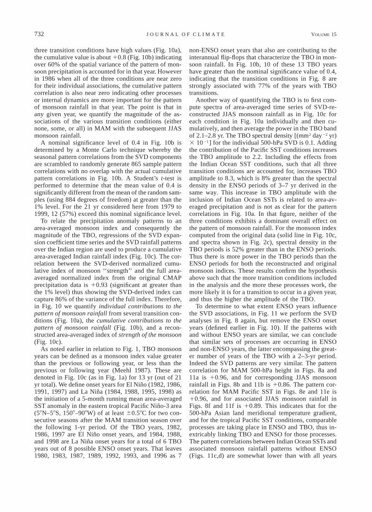
To determine to what extent ENSO years influencethe SVD associations, in Fig. 11 we perform the SVDanalyses in Fig. 8 again, but remove the ENSO onsetyears (defined earlier in Fig. 10). If the patterns withand without ENSO years are similar, we can concludethat similar sets of processes are occurring in ENSOand non-ENSO years, the latter encompassing the great-er number of years of the TBO with a 2–3-yr period.Indeed the SVD patterns are very similar. The patterncorrelation for MAM 500-hPa height in Figs. 8a and11a is 10.96, and for corresponding JJAS monsoonrainfall in Figs. 8b and 11b is 10.86. The pattern cor-relation for MAM Pacific SST in Figs. 8e and 11e is10.96, and for associated JJAS monsoon rainfall inFigs. 8f and 11f is 10.89. This indicates that for the500-hPa Asian land meridional temperature gradient,and for the tropical Pacific SST conditions, comparableprocesses are taking place in ENSO and TBO, thus in-extricably linking TBO and ENSO for those processes.The pattern correlations between Indian Ocean SSTs andassociated monsoon rainfall patterns without ENSO(Figs. 11c,d) are somewhat lower than with all years
1 APRIL 2002 733M E E H L A N D A R B L A S T E R
FIG. 11. Same as in Fig. 8 except for the El Nino and La Ninaonset years (noted in Fig. 10c) are removed. Removal of 4 El Ninoonset years and 4 La Nina onset years leaves 13 yr in this SVDanalysis.
included (Figs. 8c,d). The pattern correlations for IndianSSTs in Figs. 8c and 11c are 10.71, and for the cor-responding monsoon rainfall in Figs. 8d and 11d 10.53.In the non-ENSO years the warmer SSTs are concen-trated mostly south of India (Fig. 11c) and are associatedwith increases in JJAS Indian monsoon rainfall overmostly ocean areas, with suppressed rainfall over centraland northeastern India (Fig. 11d). Thus we concludethat the Indian Ocean does not act as strongly in unisonwith the tropical Pacific during MAM in non-ENSOyears in their contribution to the TBO as has been sug-gested by recent studies for other parts of the year (Web-ster et al. 1999; Saji et al. 1999; Chang and Li 2000;Loschnigg and Webster 2000).
5. SON to DJF transitions
Following the progression in Fig. 3, we now turn tothe subsequent Australian monsoon in DJF. Though wediscussed earlier that we identified ‘‘transition’’ con-
ditions for the Australian monsoon, it is well knownthat there is persistence from consecutive Indian to Aus-tralian monsoons, with a strong Australian monsoon of-ten following a strong Indian monsoon and vice versafor weak Indian and Australian monsoons (e.g., Shuklaand Paolino 1983; Kiladis and van Loon 1988; Websterand Yang 1992). This is represented by the strong Indianmonsoon followed by a strong convective maximum inSON over Southeast Asia leading to a strong Australianmonsoon the following DJF in the idealized depictionin Fig. 3.
To quantify this association for the full time seriesfrom 1979 to 1999, we perform SVD analyses similarto that in the Indian monsoon using conditions in SONthat are hypothesized to lead to a strong Australian mon-soon in Fig. 3d. These include SON precipitation fromthe area of maximum precipitation over Southeast Asia(108N–108S, 908–1308E); Indian Ocean SST (equator to258S, 908–1208E); and Pacific SST (208N–208S, 1508E–808W) and their respective associations with Australianmonsoon rainfall (58N–208S, 1008–1508E) in DJF.
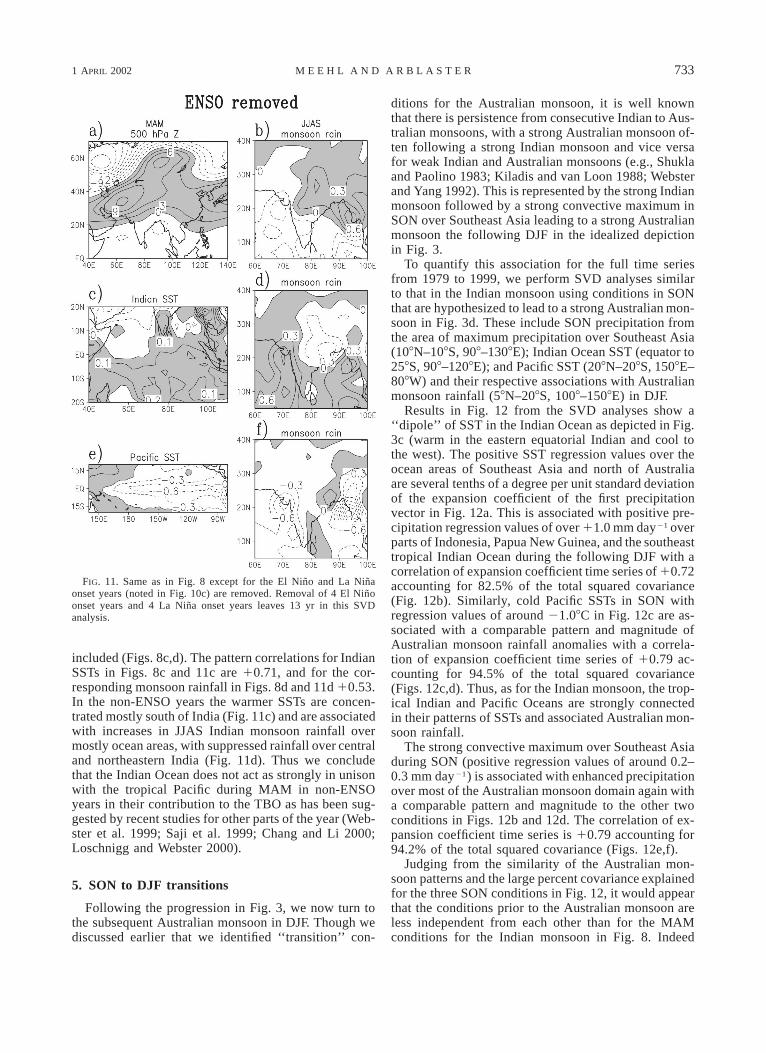
Results in Fig. 12 from the SVD analyses show a‘‘dipole’’ of SST in the Indian Ocean as depicted in Fig.3c (warm in the eastern equatorial Indian and cool tothe west). The positive SST regression values over theocean areas of Southeast Asia and north of Australiaare several tenths of a degree per unit standard deviationof the expansion coefficient of the first precipitationvector in Fig. 12a. This is associated with positive pre-cipitation regression values of over 11.0 mm day21 overparts of Indonesia, Papua New Guinea, and the southeasttropical Indian Ocean during the following DJF with acorrelation of expansion coefficient time series of 10.72accounting for 82.5% of the total squared covariance(Fig. 12b). Similarly, cold Pacific SSTs in SON withregression values of around 21.08C in Fig. 12c are as-sociated with a comparable pattern and magnitude ofAustralian monsoon rainfall anomalies with a correla-tion of expansion coefficient time series of 10.79 ac-counting for 94.5% of the total squared covariance(Figs. 12c,d). Thus, as for the Indian monsoon, the trop-ical Indian and Pacific Oceans are strongly connectedin their patterns of SSTs and associated Australian mon-soon rainfall.
The strong convective maximum over Southeast Asiaduring SON (positive regression values of around 0.2–0.3 mm day21) is associated with enhanced precipitationover most of the Australian monsoon domain again witha comparable pattern and magnitude to the other twoconditions in Figs. 12b and 12d. The correlation of ex-pansion coefficient time series is 10.79 accounting for94.2% of the total squared covariance (Figs. 12e,f).
Judging from the similarity of the Australian mon-soon patterns and the large percent covariance explainedfor the three SON conditions in Fig. 12, it would appearthat the conditions prior to the Australian monsoon areless independent from each other than for the MAMconditions for the Indian monsoon in Fig. 8. Indeed
734 VOLUME 15J O U R N A L O F C L I M A T E
FIG. 12. The first component SVD regression patterns, 1979–99, relating (a) surface temperaturesin the eastern Indian Ocean region from 258S to the equator, 908–1208E during SON [8C (unit stddev of the expansion coefficient of the first DJF precipitation vector)21] to (b) DJF precipitationover the Australian monsoon region 208S–58N, 1008–1508E [mm day21 (unit standard deviationof the expansion coefficient of the first SON surface temperature vector)21], (c) SON surfacetemperature for the area in the tropical Pacific Ocean 208S–208N, 1508E–808W [8C (unit std devof the expansion coefficient of the first DJF precipitation vector)21], to (d) DJF precipitation overthe Australian monsoon region 208S–58N, 1008–1508E [mm day21 (unit std dev of the expansioncoefficient of the first surface temperature vector)21], (e) SON precipitation over the SoutheastAsian area 108S–108N, 908–1308E [mm day21 (unit std dev of the expansion coefficient of thefirst DJF precipitation vector)21], to (d) DJF precipitation over the Australian monsoon region208S–58N, 1008–1508E [mm day21 (unit std dev of the expansion coefficient of the first SONSoutheast Asian precipitation vector)21]. Note that the regression plots can extend beyond theirrespective areas used in the SVD calculation. Shaded areas indicate positive values.
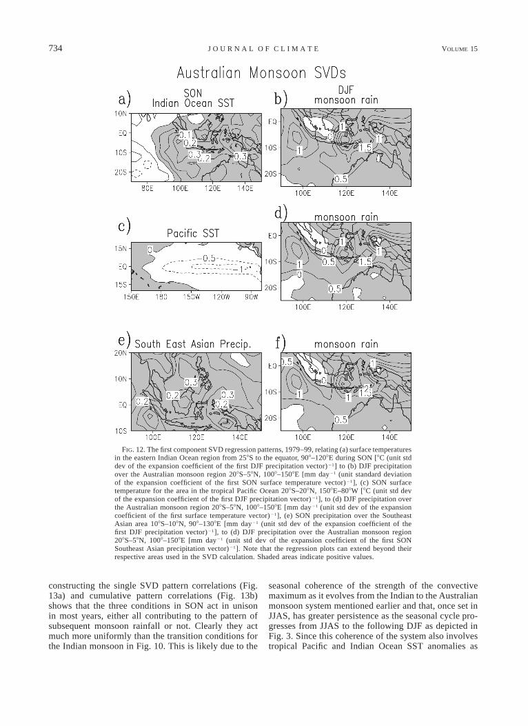
constructing the single SVD pattern correlations (Fig.13a) and cumulative pattern correlations (Fig. 13b)shows that the three conditions in SON act in unisonin most years, either all contributing to the pattern ofsubsequent monsoon rainfall or not. Clearly they actmuch more uniformly than the transition conditions forthe Indian monsoon in Fig. 10. This is likely due to the
seasonal coherence of the strength of the convectivemaximum as it evolves from the Indian to the Australianmonsoon system mentioned earlier and that, once set inJJAS, has greater persistence as the seasonal cycle pro-gresses from JJAS to the following DJF as depicted inFig. 3. Since this coherence of the system also involvestropical Pacific and Indian Ocean SST anomalies as
1 APRIL 2002 735M E E H L A N D A R B L A S T E R
FIG. 13. (a) Time series, 1979–99, of individual anomaly patterncorrelations for the regional (Indian Ocean SST and Southeast Asianprecipitation) and large-scale (Pacific surface temperatures) SONSVD-derived conditions from Fig. 12 with observed DJF Australianmonsoon rainfall patterns for the area 208S–58N, 1008–1508E, (b)cumulative anomaly pattern correlations for Australian monsoon rain-fall combining the three conditions in (a); nominal significance levelof 0.40 (marked in Fig. with thin solid line) is determined by a MonteCarlo technique described in the text; (c) time series of an index ofAustralian monsoon strength (area-averaged over Australian monsoonregion, all points, 208S–58N, 1008–1508E) of the cumulative precip-itation patterns in (b) derived from the SVD analysis normalized bytheir respective std dev (dash–dot line), and the full area-averagednormalized precipitation index over the same region calculated fromthe original precipitation data (solid line as in Fig. 1b). EN and LNonset years defined in text are denoted beneath the correspondingyears. Solid dots in (b) and (c) indicate relatively strong and weakmonsoon years in relation to previous and following years for theobserved index in (c). Warm (W, western Indian Ocean warmer thaneast, ‘‘positive dipole’’) and cold (C, western Indian Ocean colderthan east, ‘‘negative dipole’’) extreme SST dipole years from Saji etal. (1999) also noted below years at bottom.
shown in Figs. 12 and 13, these must be related to upper-ocean temperature anomalies and ocean dynamics. Thisis addressed in a subsequent paper (Meehl et al. 2002,manuscript submitted to J. Climate).
The reconstructed area-averaged rainfall index in Fig.13c from the SVD patterns is highly correlated with the
total area-averaged index from the original precipitationdata (10.97) indicating, as for the Indian monsoon rain-fall data, that the SVD reconstructions can reproducemuch of the original time series of monsoon strength(94% of the variance) using just the first SVD com-ponents. The tendency for persistence from Indian toAustralian monsoon noted above can be demonstratedby correlating the JJAS Indian monsoon area-averagedprecipitation index (Fig. 10c) with the following DJFAustralian monsoon area-averaged precipitation index(Fig. 13c). This value is 10.55, which is significant atthe 1% level corroborating earlier results that in manyyears a strong Indian monsoon is followed by a strongAustralian monsoon, and vice versa for weak monsoons.Also it is clear from Fig. 3 why there is little persistencefrom Australian monsoon to subsequent Indian monsoonsince the TBO transition period is across the seasonsMAM–JJAS.
As noted above, the SST dipole in the Indian Oceanwith maximum values in the SON season is seen hereto be an integral part of the TBO and is a consequenceof coupled air–sea interaction directly involving the In-dian and Australian monsoons. Extreme dipole modeevents from Saji et al. (1999) are 1982, 1994, and 1997(warm or ‘‘positive dipole’’ with positive SST anoma-lies in the western Indian and negative in the east, op-posite in sign to the depiction in Figs. 3 and 12), and1984, 1992, and 1996 (cold or ‘‘negative’’ dipole withsigns as depicted in Figs. 3 and 12). Thus the ‘‘W’’ inFig. 13c refers to positive dipole (warm west and cooleast), and the ‘‘C’’ to negative dipole (cool east andwarm west). For those 6 strong dipole mode events, 5are significantly accounted for by the Indian Ocean SSTSVD pattern in Fig. 13a (dashed line) with values nearor greater than 10.4 (all but 1984). All are also seento act in unison with the tropical Pacific in Fig. 13a(comparable evolution of dashed and dotted lines),though only 1982 and 1997 are El Nino onset years,and 1984 is a La Nina onset year. Therefore, half (three)of the extreme Indian Ocean dipole years are non-ENSOonset years consistent with previous observations thatextreme Indian Ocean dipole years can occur withoutan extreme ENSO year. This also has been noted tooccur in a coupled GCM (Iizuka et al. 2000). However,Fig. 13a does indicate a linkage to the tropical Pacific,through coupled interactions involving the large-scaleeast–west circulation (WWC and EWC) involved withthe Asian–Australian monsoon system and coupledocean dynamics (Fig. 3). It is also worth noting that theIndian Ocean dipole pattern with significant pattern cor-relations (with subsequent Australian monsoon rainfall)above 10.4 in Fig. 13a occurs in other years as well(1985, 1986, 1988, 1991, 1995, and 1998).
For the reconstructed Australian monsoon precipita-tion index in Fig. 13c, all three extreme warm or positivedipole events are associated with below-normal Austra-lian monsoon rainfall, and two out of three cold or neg-ative dipole events occur in years with above-normal

736 VOLUME 15J O U R N A L O F C L I M A T E
Australian monsoon rainfall (all but 1992). This sup-ports the connection between the Indian Ocean SSTdipole pattern in SON with the strength of the DJFAustralian monsoon and the TBO.
If TBO years are defined in a similar way to the Indianmonsoon (denoted by the solid dots in Fig. 13c), 6 ofthe 11 TBO years are significantly accounted for by thecumulative pattern correlations in Fig. 13b (values nearor above 10.4). It was noted earlier that there is seasonalpersistence from Indian to Australian monsoon as in-dicated by an overall correlation between Indian and thesubsequent Australian monsoon of 10.55. This is alsoseen in the TBO years. For the 13 TBO years definedfor the Indian monsoon in Fig. 10c, only 12 are eligiblefor continuation to the Australian monsoon (even though1998 is an above-normal Australian monsoon, we can-not define it as a TBO year relatively stronger than thepreceding and following years since the precipitationdata end in October 1999 and we do not have the 1999Australian monsoon data). For those 12 TBO Indianmonsoon years, 8 or 67% correspond to like sign TBOyears in the Australian monsoon, 4 relatively strong(1980, 1983, 1988, 1996) and 4 relatively weak (1982,1984, 1989, 1997). Of those 8, only 4 are ENSO onsetyears (1982 and 1997 El Nino, 1984 and 1988 La Nina).This demonstrates that there are years other than ENSOextremes that contribute to the TBO.
To address the contribution of ENSO versus non-ENSO onset years to the TBO in the Australian mon-soon, a similar SVD calculation to that in Fig. 12 isperformed without the ENSO onset years (not shown).As in the Indian monsoon non-ENSO onset years, thereare very similar patterns to that for the full set of years,with pattern correlations for Pacific SSTs (Fig. 12c) of10.89, with monsoon rainfall associated with PacificSSTs (Fig. 12d) of 10.53, pattern correlations for south-east Asian precipitation (Fig. 12e) of 10.72, and withmonsoon rainfall associated with southeast Asian pre-cipitation (Fig. 12f) of 10.68. Also similar to the Indianmonsoon, The Indian Ocean SST relationships are notas strong for all years and non-ENSO onset years withpattern correlations for Indian SSTs (Fig. 12a) of 10.53,and with subsequent Australian monsoon rainfall (Fig.12b) of 10.41. Also, as in the Indian monsoon non-ENSO onset years, the maximum positive SST valuesfor SON are centered more in the southeastern part ofthe domain (not shown). Thus, ENSO onset years aretied strongly to the dipole pattern in SON, but non-ENSO onset years are not so strongly linked.
6. Time evolution
To examine the time evolution of the conditions as-sociated with the TBO, we regress the precipitation SVDexpansion coefficient time series computed for JJASprecipitation and MAM 500-hPa height (patterns inFigs. 8a,b), and JJAS precipitation and Indian OceanSST (patterns in Figs. 8c,d) against precipitation, sur-
face wind, and surface temperature data for seasons de-picted in Fig. 3 and results are shown in Figs. 14 and15, respectively. It was noted that Indian and PacificSST SVD patterns for all years are similar, so only theIndian Ocean SST SVD association with JJAS precip-itation is used here.
The JJAS Indian monsoon precipitation SVD expan-sion coefficient time series derived for MAM 500-hPaheight anomalies over Asia regressed against surfacewind, surface temperature, and precipitation is shownin Fig. 14. If only values exceeding a 95% significancelevel were plotted, the number of vectors and contourswould be reduced. However, we choose to plot valuesat every grid point since the time series are relativelyshort and we wish to address the physical significanceof the plotted quantities (Nicholls 2001).
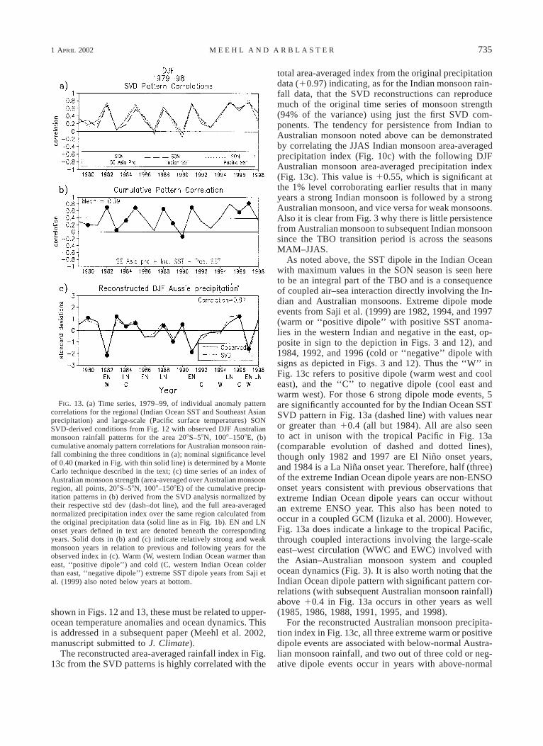
Note that the sign and pattern for JJAS precipitationin Fig. 14e closely resembles the sign and pattern inFig. 8b (as it must since they are derived from the sameexpansion coefficient time series, with the heteroge-neous association in Fig. 8 and homogeneous in Fig.14), with enhanced precipitation over much of northernIndia, Bangladesh, and Burma. Also note that the sur-face temperature regressions in Fig. 14d for MAM (withwarm conditions over much of Asia) are comparable interms of sign and pattern to Fig. 9. This shows that thesign convention of the regressions in Fig. 14 is consis-tent with the physical interpretation of Figs. 8 and 9.
Conditions leading up to the precipitation pattern inFig. 14e can be seen to involve a positive precipitationmaximum with regression values of over 0.3 mm day21
over the equatorial western Pacific Ocean near 1508Eto the date line in the DJF-1 (Fig. 14a). As in Fig. 4for the simultaneous associations, positive values extendover northern Australia, but also reach farther west overPapua New Guinea in association with westerly windanomalies there. In fact the precipitation is enhancedfar enough west that the regressed SST pattern in Fig.14b shows negative anomalies in the eastern equatorialPacific opposite to that in the idealized schematic inFig. 3.
There is suppressed precipitation over Malaysia andthe Indian Ocean, with regression values of severaltenths of a mm day21. Though this is two seasons re-moved from the SVD calculation for JJAS, this patternalso resembles the contemporaneous SVD for DJF inFig. 4. This indicates that the associations in a givenseason and the relationships to following seasons arerobust.
The pattern of convective heating anomalies stretch-ing from eastern Africa to the western equatorial Pacificwas noted earlier to be associated with an anomalousridge of positive 500-hPa height anomalies over Asia,and warmer Asian land temperatures. Similarly, anom-alously warm land temperatures with regression valuesof greater than 10.58C appear over much of south Asiain DJF-1 (Fig. 14b) as was noted for the contempora-neous relationship in Fig. 7. In association with the
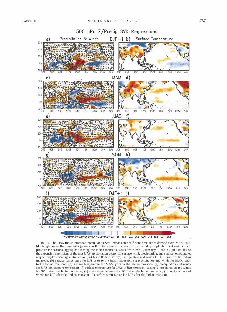
1 APRIL 2002 737M E E H L A N D A R B L A S T E R
FIG. 14. The JJAS Indian monsoon precipitation SVD expansion coefficient time series derived from MAM 500-hPa height anomalies over Asia (pattern in Fig. 8b) regressed against surface wind, precipitation, and surface tem-perature for seasons lagging and leading the Indian monsoon. Units are in m s21, mm day21, and 8C (unit std dev ofthe expansion coefficient of the first JJAS precipitation vector for surface wind, precipitation, and surface temperature,respectively)21. Scaling vector above part (c) is 0.75 m s21. (a) Precipitation and winds for DJF prior to the Indianmonsoon; (b) surface temperature for DJF prior to the Indian monsoon; (c) precipitation and winds for MAM priorto the Indian monsoon; (d) surface temperature for MAM prior to the Indian monsoon; (e) precipitation and windsfor JJAS Indian monsoon season; (f ) surface temperature for JJAS Indian monsoon season; (g) precipitation and windsfor SON after the Indian monsoon; (h) surface temperature for SON after the Indian monsoon; (i) precipitation andwinds for DJF after the Indian monsoon; (j) surface temperature for DJF after the Indian monsoon.
738 VOLUME 15J O U R N A L O F C L I M A T E
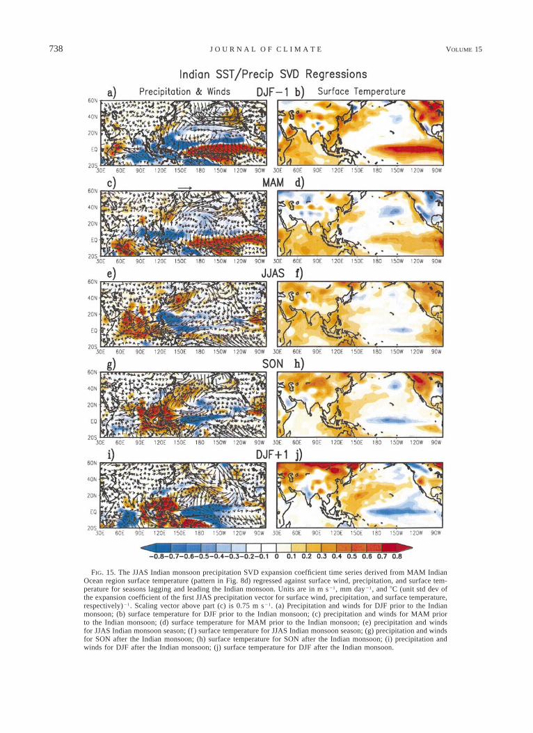
FIG. 15. The JJAS Indian monsoon precipitation SVD expansion coefficient time series derived from MAM IndianOcean region surface temperature (pattern in Fig. 8d) regressed against surface wind, precipitation, and surface tem-perature for seasons lagging and leading the Indian monsoon. Units are in m s21, mm day21, and 8C (unit std dev ofthe expansion coefficient of the first JJAS precipitation vector for surface wind, precipitation, and surface temperature,respectively)21. Scaling vector above part (c) is 0.75 m s21. (a) Precipitation and winds for DJF prior to the Indianmonsoon; (b) surface temperature for DJF prior to the Indian monsoon; (c) precipitation and winds for MAM priorto the Indian monsoon; (d) surface temperature for MAM prior to the Indian monsoon; (e) precipitation and windsfor JJAS Indian monsoon season; (f ) surface temperature for JJAS Indian monsoon season; (g) precipitation and windsfor SON after the Indian monsoon; (h) surface temperature for SON after the Indian monsoon; (i) precipitation andwinds for DJF after the Indian monsoon; (j) surface temperature for DJF after the Indian monsoon.
1 APRIL 2002 739M E E H L A N D A R B L A S T E R
precipitation anomalies, there are westerly wind anom-alies of about 10.5 m s21 in the western Pacific, andsoutheasterly anomalies over the equatorial IndianOcean.
In MAM (Fig. 14c) the lagged pattern of regressedtropical precipitation anomalies is similar to the simul-taneous SVD calculation in Fig. 6b. There are enhancedprecipitation regression values of several tenths of amm day21 over the western Indian Ocean and parts ofIndochina, and larger values of greater than 10.6mm day21 in the western Pacific east of about 1608E(see Ju and Slingo 1995). There is suppressed precip-itation north of Papua New Guinea, with regression val-ues of several tenths of a mm day21. Similarly, thistropical precipitation pattern is associated with positive500-hPa height anomalies over Asia (Fig. 8a) and anom-alously warm Asian land temperatures with regressionvalues greater than 10.78C (Fig. 14d) similar to thosefor the contemporaneous relationship in Fig. 7. Bothhave an enhanced surface temperature gradient oversouth Asia. Anomalous westerly wind regression valuesof about 10.3 m s21 continue over the western equa-torial Pacific with southwesterly values of about thatsame magnitude over the Arabian Sea, and easterlyanomaly winds of about 0.5 m s21 along the equator inthe western Indian Ocean.
The JJAS patterns in Figs. 14e,f show enhanced pre-cipitation over northeastern India and Bangladesh asnoted above with strengthened southwesterly flow overthe Arabian Sea. In addition, there is suppressed pre-cipitation over the Indian Ocean, eastern Asia, Malaysia,and parts of Indonesia, while there is enhanced precip-itation over Japan, the western Pacific northeast of thePhilippines, and along the ITCZ in the Pacific. Thisenhanced precipitation component has almost a hemi-spheric ITCZ-like aspect with a band of positive pre-cipitation regression values extending from India acrossthe South China Sea and east of the Philippines. Thereare strengthened south and southwest winds across theArabian Sea with regression values of about 0.3 m s21,and westerly anomalies of about twice that magnitudein the western tropical Pacific. SSTs in the central equa-torial Pacific are anomalously warm but with small re-gression values of about 10.2, while SSTs in the north-ern Indian Ocean are anomalously cool.
The SON season in Figs. 14g,h shows positive pre-cipitation regression values of roughly 10.4 mm day21
over eastern China and north of the equator in the Pa-cific, easterly regression values of about 0.5 m s21 inthe equatorial eastern Indian Ocean, and westerly anom-alies of about that same magnitude near the date line inthe Pacific associated with small positive SST regressionvalues of 10.48C in the central and eastern tropicalPacific. There is the suggestion of a weak positive dipoleof SSTs and easterly wind anomalies across the equa-torial Indian Ocean, with somewhat warmer SSTs in thewest and cooler in the east. By DJF following the mon-soon (Figs. 14i,j), there are easterly anomaly winds in
the far western equatorial Pacific, easterly anomalywinds south of the equator in the Indian Ocean, and amixture of positive and negative precipitation anomaliesin the Australian monsoon region.
The lagged precipitation, wind, and SST regressionsin Fig. 14 are consistent with the simultaneous calcu-lations for DJF and MAM in Figs. 4–7 but differ insome respects with the hypothesized evolution in Fig.3. This suggests that the enhanced meridional temper-ature gradient mechanism depicted in Fig. 14 may notwork in concert with the SST-driven ones. To explorethe latter in Fig. 15, the SVD expansion coefficient timeseries from the JJAS Indian monsoon rainfall calculatedusing the MAM Indian SST in Figs. 8c,d are regressedagainst surface winds, temperatures, and precipitation.Figure 8d can be compared to be similar (as it must be,as noted for Fig. 14e) with a comparable sign convectionto Fig. 15e. But the larger domain is seen to show en-hanced precipitation not only over parts of southernIndia and Bangladesh as was seen in Fig. 8d, but alsoover much of the Indian Ocean region as well withregression values greater than 10.4 mm day21. The In-dian Ocean SST anomalies in MAM are positive withlargest values south of about 108N in Fig. 15d. Theanomalously warm SSTs over the Indian Ocean in MAM(Fig. 15d) are comparable to the values shown in Fig.8c.
The DJF preceding the Indian monsoon shows a weakAustralian monsoon with negative precipitation regres-sion values of at least 20.6 mm day21 over almost theentire Australian monsoon domain in Fig. 15a, witheasterly anomaly wind regression values of around 0.7m s21 along the equatorial Indian Ocean with somewhatweaker easterly anomalies in the far western equatorialPacific. There are also westerly anomaly wind regres-sion values of nearly 0.8 m s21 associated with anom-alously warm SSTs in the eastern and central equatorialPacific (Fig. 15b). In MAM there is suppressed precip-itation (roughly 20.4 mm day21) near 108N stretchingfrom East Africa to about 1208W, while northeasterlyanomaly wind regression values of about 0.4 m s21 con-tinue in the western equatorial Pacific and westerlyanomaly winds appear in the far western equatorial In-dian Ocean (Fig. 15c). The Indian Ocean is anomalouslywarm as is the central and eastern equatorial Pacific(Fig. 15d) with regression values of greater than 0.48C.There is little consistent surface temperature anomalypattern over southern Asia.
As noted above, in JJAS (Fig. 15e) there is enhancedprecipitation over most of India, Bangladesh, and theIndian Ocean (some regression values exceed 10.8mm day21). Since most of the anomalous precipitationlies over the Indian Ocean in Fig. 15e, the main anom-alous surface wind convergence is near the equator inthe Indian Ocean, with anomalous westerly regressionvalues of about 0.4 m s21 in the western Indian Ocean,and anomalous easterlies with regression values ofaround 0.5 m s21 in the eastern Indian Ocean stretching
740 VOLUME 15J O U R N A L O F C L I M A T E
across most of Southeast Asia into the western PacificOcean. Even though there is enhanced Indian monsoonrainfall in Fig. 15e, there are easterly wind anomaliesover the Arabian Sea where one would expect to seesouthwesterly anomalies with stronger inflow as in Fig.14e. To examine this response, GCM sensitivity exper-iments with specified SST anomalies over the IndianOcean show that greater precipitation over the IndianOcean has a regional effect on winds that can produceeasterly anomalies over the Arabian Sea even with en-hanced rainfall over India (MEAR1).
In Fig. 15f, SSTs have transitioned from positive inMAM to negative in JJAS in the central equatorial Pa-cific and small negative SST anomalies have just ap-peared off the coast of equatorial Africa in the westernIndian Ocean in association with the implied enhancedupwelling from the westerly wind anomalies there.
In SON (Figs. 15g,h) the strong monsoon convectivemaximum from JJAS traverses east and south encoun-tering anomalously warm SSTs in its path and coversmost of Southeast Asia with positive precipitationanomalies with regression values mostly greater than10.7 mm day21. There is surface wind convergenceassociated with that convective maximum, with westerlyanomalies over much of the equatorial Indian Ocean,and easterly anomalies over the western Pacific, bothwith regression values of greater than 0.5 m s21. Anegative SST dipole in the Indian Ocean has small neg-ative anomalies in the west and positive anomalies inthe east, and there are strengthening negative SST re-gression values in the equatorial central Pacific ofroughly 20.58C.
By DJF11 after the Indian monsoon, the strong con-vective maximum (with regression values mostly greaterthan 0.7 mm day21) has become established over mostof the Australian monsoon domain (Fig. 15i) and west-erly anomaly winds with regression values of greaterthan 0.5 m s21 now shifted south of the equator in thetropical southeastern Indian Ocean. There is evidenceof westerly anomaly wind regression values of about0.3 m s21 in the far western equatorial Pacific witheasterly anomaly wind regression values of about 0.7m s21 east of 1508E. As mentioned earlier, this seasonalevolution is similar for the Pacific SVD projection forall years (not shown) indicating that the Indian and Pa-cific are linked in many years through large-scale east–west atmospheric circulation anomalies (the WWC andEWC) associated with the movement of the convectivemaximum from the Indian to Australian monsoon, andits coupled interactions with the ocean.
In comparing the sequences depicted in Figs. 14 and15 with the idealized evolution of the TBO in Fig. 3, anumber of interesting aspects emerge. First, for the link-ages between the tropical convective heating anomalies,500-hPa circulation, and land temperature anomalies,there are differences in the connections to the tropicalPacific. This also relates to where, exactly, precipitationanomalies occur over the south Asian monsoon region.
The apparent contribution of anomalous meridionaltemperature gradients prior to the Indian monsoon as-sociated with tropical convective heating anomalies ismainly related to enhanced precipitation over some landareas of south Asia (northeast India, Bangladesh, andBurma). They apparently can act independently fromforcing from the tropical Pacific since the sense of theevolution of SST anomalies in the tropical Pacific isopposite between Figs. 14 and 15. This is not a resultof a random choice of sign convention since, as notedabove, the sign of the patterns in Figs. 14 and 15 matchthose of the SVD patterns in Figs. 4–8 for consistentphysical interpretation. Additionally, the Asian landtemperature anomalies in Fig. 14 are not biennial, withpositive land temperature anomalies in DJF-1 andDJF11. However, since the two sequences presumablyrepresent components of the actual evolution and arenot orthogonal, there is overlap as could be expectedfrom such a coupled system. In any given year in theTBO one or the other of the processes can contributeto the actual patterns of rainfall as seen in Fig. 10a.Since the more land-based precipitation pattern in Fig.14e and the Indian Ocean–based pattern in Fig. 15e areassociated with different evolutions of Pacific SSTs, itis no surprise that in any given monsoon year the linkagewith the tropical Pacific can be intermittent.
The question still remains concerning whether theland-based meridional temperature gradient mechanismor the SST-based mechanisms could, independently,produce the precipitation anomaly patterns in the laggedregression plots in Figs. 14 and 15. This question isaddressed directly through the use of GCM sensitivityexperiments by MEAR1. Results show that indeed eachmechanism can produce comparable patterns of precip-itation response in Figs. 14 and 15, and that the SST-based mechanisms are relatively stronger. Yet, as shownin Figs. 10 and 13, each mechanism can make partialcontributions in any given year.
In any case, the circulation-related sequence in Fig.14 appears to produce a more anomalous hemisphericprecipitation pattern during the monsoon season, withthe Indian monsoon enhancement part of an ITCZ-likepositive precipitation anomaly pattern stretching east ofthe Philippines. However, the more Indian Ocean–basedprecipitation anomaly pattern in Fig. 15e has an east–west character, with enhanced precipitation over mostof the Indian sector and suppressed precipitation overthe western Pacific east of the Philippines. This strongconvective maximum in the Indian sector then pro-gresses in Fig. 15 much as depicted in Fig. 3, remainingstrong in its southeastward progression across SoutheastAsia in SON culminating in a strong Australian mon-soon in the following DJF. Conversely, the meridionaltemperature gradient pattern shows more of an overallweakened convective maximum progressing southeast-ward with the seasonal cycle as indicated by the negativeprecipitation regression values in that region.
It is also clear from the surface winds that there are
1 APRIL 2002 741M E E H L A N D A R B L A S T E R
ocean dynamical linkages. Anomalous winds in the farwestern equatorial Pacific in DJF in Fig. 15 precedetransitions of SSTs in the central and eastern equatorialPacific, with the transition starting in MAM and op-posite sign SST anomalies becoming established inJJAS. Thus a preliminary answer to the question of‘‘what makes the TBO flip from one year to the next’’directly involves coupled ocean–atmosphere interactionin the Australian monsoon region in DJF, which wouldtrigger oceanic Kelvin waves that affect the thermoclinefarther east in the Pacific to induce an SST transitionin subsequent months. In addition, surface wind anom-alies in the equatorial Indian Ocean are seen to initiatethe Indian Ocean SST dipole pattern starting half a yearlater in JJAS, peaking in SON, and making the fulltransition to opposite sign anomalies by the subsequentDJF. We directly address the question of ocean dynamicsin Meehl et al. (2002, manuscript submitted to J. Cli-mate). In that paper we examine composites of TBOtransitions in observed atmospheric and upper-oceandata, and show that oceanic Rossby waves (Webster etal. 1999) also play a role in these transitions. Loschnigget al. (2002, manuscript submitted to J. Climate) showsimilar results from an analysis of a global coupled mod-el.
7. Discussion and conclusions
In Fig. 3 we presented a hypothesized series of cou-pled interactions to account for conditions associatedwith TBO transitions. The various contemporaneous andlagged SVD and composite analyses have raised someinteresting issues. First, due to the well-known seasonalpersistence from Indian to Australian monsoon, the mostimportant TBO transitions occur from MAM to JJAS.Those transitions account first for the interannual var-iations of the patterns of monsoon rainfall in JJAS, andthen for a majority of years of Australian monsoon rain-fall strength. However, the JJAS rainfall over Austral-asia, that is dynamically important for the large-scaleclimate system in the Indian and Pacific sectors, coversa huge area of land and ocean. In this context, the Indianmonsoon, strictly over India and more broadly inter-preted as rainfall over south Asian land areas, is onlyon the northwestern edge of the vast maximum of JJASrainfall that extends over much of the tropical IndianOcean and east to Southeast Asia. Any analysis of thedynamically important mechanisms must account forvariations in this entire pattern, not just small regionalpieces of it. We saw that the regional pieces (such asIndia) have rainfall that is influenced by conditions andassociated rainfall anomalies over much larger regions.
For the tropical Pacific and Indian Ocean conditions,it was noted that the SST transitions start to occur twoseasons later in the Indian Ocean in conjunction withthe Indian monsoon (JJAS) compared to the central andeastern Pacific which begins the transition process inassociation with the Australian monsoon (DJF). In the
Pacific the SST transition is complete by the followingIndian monsoon in JJAS, and finishes in the IndianOcean by the following Australian monsoon in DJF. Thisis due to the nature of the coupled wind forcing andocean dynamical response along with the seasonal evo-lution of the convective maximum as it traverses fromthe Indian region to the Australian region. As part ofthis seasonal evolution and associated coupled windforcing, in conjunction with ocean dynamics, the SSTdipole in the Indian Ocean starts to appear as part ofthis transition in the Indian Ocean in JJAS. The SSTtransition is part way completed in SON when the IndianOcean SST dipole is most apparent, and is fully tran-sitioned by DJF when the dipole gives way to SSTanomalies in the tropical Indian Ocean of one sign andthe influence of the Australian monsoon is most evident.There is a linkage between the Indian and Pacific Oceansdue to the coupling inherent in the large-scale east–westatmospheric circulations (the WWC and EWC) asso-ciated with the seasonal movement of the convectivemaximum over Australasia, but with the 6-month lagsinvolved with the seasonal cycle and coupled atmo-sphere–ocean interactions. These linkages account formuch of the rainfall variability over the tropical IndianOcean, and parts of western India, Bangladesh, and east-ern China (Figs. 8, 15). The dynamical interactions re-sponsible for SST transitions in the Indian Ocean beginwith the Indian monsoon and end with the subsequentAustralian monsoon. In the Pacific SST transitions beginwith the Australian monsoon and end with the followingIndian monsoon. The Indian and Pacific Oceans thushave a certain seasonal symmetry with the SST tran-sitions occurring half a year apart.
It has been noted that the influence of the tropicalPacific SST anomalies on Indian monsoon rainfall hasdiminished since the late 1970s (Krishna Kumar et al.1999). Other changes in base state apparently have oc-curred in the Indian Ocean to alter certain monsoonlinkages with conditions such as SST (Clark et al. 2000).Since our data only cover the period since this apparentchange, we note that both the Indian and Pacific SVDpatterns are similar (Fig. 8) with a greater link to rainfallover the Indian Ocean with peripheral (but regionallyimportant) influences over India and other south Asianland areas. The importance of the Indian Ocean SSTsto subsequent patterns of Indian monsoon rainfall wasindicated by the fact that the squared covariance ac-counted for was 58% for the MAM Indian SST/JJASmonsoon rainfall SVD association, but only 39% foreach of the Pacific and 500-hPa height associations (Fig.8). Part of the reason for the somewhat reduced ampli-tude for the Pacific SSTs is that there is an impliedtransition from MAM to JJAS in the Pacific that reducesseasonal persistence, while in the Indian Ocean the signof SST anomalies is mostly the same from MAM toJJAS, with the transition occurring over the next twoseasons as part of the SST dipole.
It was also noted that the rainfall over the Indian
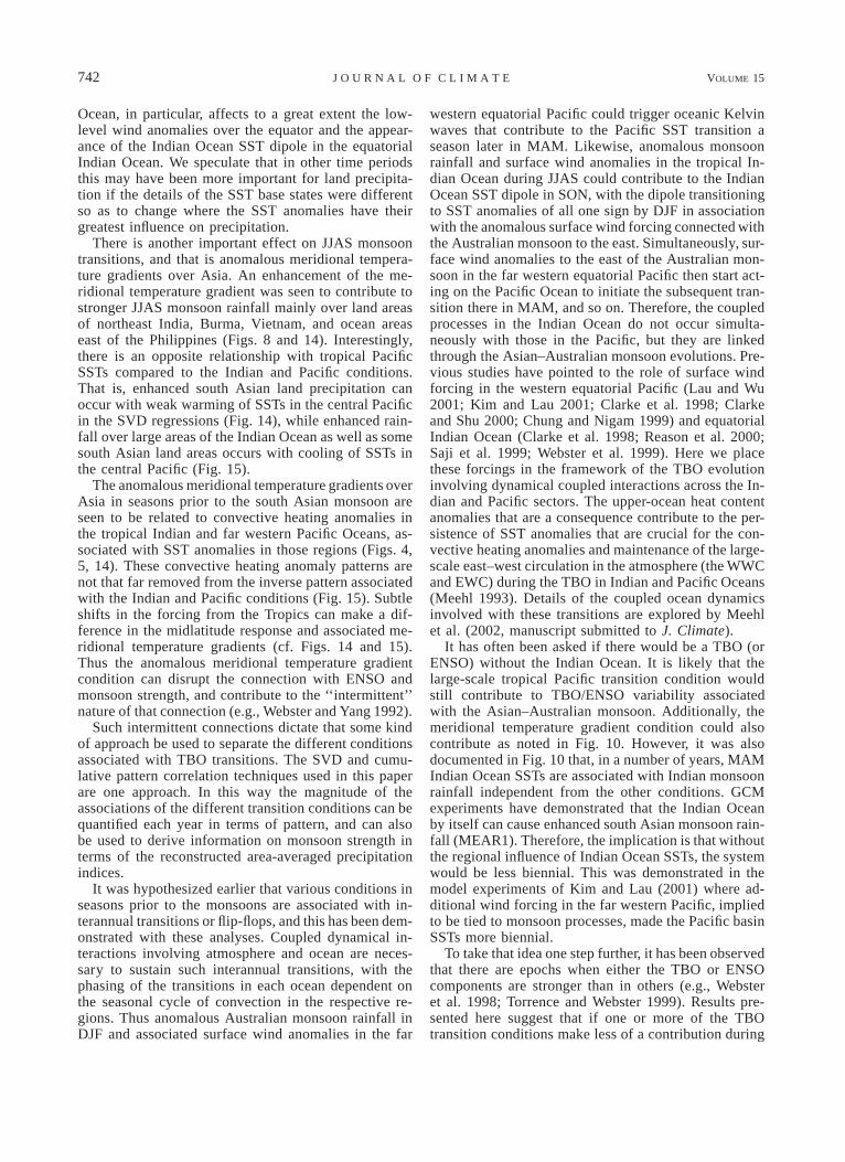
742 VOLUME 15J O U R N A L O F C L I M A T E
Ocean, in particular, affects to a great extent the low-level wind anomalies over the equator and the appear-ance of the Indian Ocean SST dipole in the equatorialIndian Ocean. We speculate that in other time periodsthis may have been more important for land precipita-tion if the details of the SST base states were differentso as to change where the SST anomalies have theirgreatest influence on precipitation.
There is another important effect on JJAS monsoontransitions, and that is anomalous meridional tempera-ture gradients over Asia. An enhancement of the me-ridional temperature gradient was seen to contribute tostronger JJAS monsoon rainfall mainly over land areasof northeast India, Burma, Vietnam, and ocean areaseast of the Philippines (Figs. 8 and 14). Interestingly,there is an opposite relationship with tropical PacificSSTs compared to the Indian and Pacific conditions.That is, enhanced south Asian land precipitation canoccur with weak warming of SSTs in the central Pacificin the SVD regressions (Fig. 14), while enhanced rain-fall over large areas of the Indian Ocean as well as somesouth Asian land areas occurs with cooling of SSTs inthe central Pacific (Fig. 15).
The anomalous meridional temperature gradients overAsia in seasons prior to the south Asian monsoon areseen to be related to convective heating anomalies inthe tropical Indian and far western Pacific Oceans, as-sociated with SST anomalies in those regions (Figs. 4,5, 14). These convective heating anomaly patterns arenot that far removed from the inverse pattern associatedwith the Indian and Pacific conditions (Fig. 15). Subtleshifts in the forcing from the Tropics can make a dif-ference in the midlatitude response and associated me-ridional temperature gradients (cf. Figs. 14 and 15).Thus the anomalous meridional temperature gradientcondition can disrupt the connection with ENSO andmonsoon strength, and contribute to the ‘‘intermittent’’nature of that connection (e.g., Webster and Yang 1992).
Such intermittent connections dictate that some kindof approach be used to separate the different conditionsassociated with TBO transitions. The SVD and cumu-lative pattern correlation techniques used in this paperare one approach. In this way the magnitude of theassociations of the different transition conditions can bequantified each year in terms of pattern, and can alsobe used to derive information on monsoon strength interms of the reconstructed area-averaged precipitationindices.
It was hypothesized earlier that various conditions inseasons prior to the monsoons are associated with in-terannual transitions or flip-flops, and this has been dem-onstrated with these analyses. Coupled dynamical in-teractions involving atmosphere and ocean are neces-sary to sustain such interannual transitions, with thephasing of the transitions in each ocean dependent onthe seasonal cycle of convection in the respective re-gions. Thus anomalous Australian monsoon rainfall inDJF and associated surface wind anomalies in the far
western equatorial Pacific could trigger oceanic Kelvinwaves that contribute to the Pacific SST transition aseason later in MAM. Likewise, anomalous monsoonrainfall and surface wind anomalies in the tropical In-dian Ocean during JJAS could contribute to the IndianOcean SST dipole in SON, with the dipole transitioningto SST anomalies of all one sign by DJF in associationwith the anomalous surface wind forcing connected withthe Australian monsoon to the east. Simultaneously, sur-face wind anomalies to the east of the Australian mon-soon in the far western equatorial Pacific then start act-ing on the Pacific Ocean to initiate the subsequent tran-sition there in MAM, and so on. Therefore, the coupledprocesses in the Indian Ocean do not occur simulta-neously with those in the Pacific, but they are linkedthrough the Asian–Australian monsoon evolutions. Pre-vious studies have pointed to the role of surface windforcing in the western equatorial Pacific (Lau and Wu2001; Kim and Lau 2001; Clarke et al. 1998; Clarkeand Shu 2000; Chung and Nigam 1999) and equatorialIndian Ocean (Clarke et al. 1998; Reason et al. 2000;Saji et al. 1999; Webster et al. 1999). Here we placethese forcings in the framework of the TBO evolutioninvolving dynamical coupled interactions across the In-dian and Pacific sectors. The upper-ocean heat contentanomalies that are a consequence contribute to the per-sistence of SST anomalies that are crucial for the con-vective heating anomalies and maintenance of the large-scale east–west circulation in the atmosphere (the WWCand EWC) during the TBO in Indian and Pacific Oceans(Meehl 1993). Details of the coupled ocean dynamicsinvolved with these transitions are explored by Meehlet al. (2002, manuscript submitted to J. Climate).
It has often been asked if there would be a TBO (orENSO) without the Indian Ocean. It is likely that thelarge-scale tropical Pacific transition condition wouldstill contribute to TBO/ENSO variability associatedwith the Asian–Australian monsoon. Additionally, themeridional temperature gradient condition could alsocontribute as noted in Fig. 10. However, it was alsodocumented in Fig. 10 that, in a number of years, MAMIndian Ocean SSTs are associated with Indian monsoonrainfall independent from the other conditions. GCMexperiments have demonstrated that the Indian Oceanby itself can cause enhanced south Asian monsoon rain-fall (MEAR1). Therefore, the implication is that withoutthe regional influence of Indian Ocean SSTs, the systemwould be less biennial. This was demonstrated in themodel experiments of Kim and Lau (2001) where ad-ditional wind forcing in the far western Pacific, impliedto be tied to monsoon processes, made the Pacific basinSSTs more biennial.
To take that idea one step further, it has been observedthat there are epochs when either the TBO or ENSOcomponents are stronger than in others (e.g., Websteret al. 1998; Torrence and Webster 1999). Results pre-sented here suggest that if one or more of the TBOtransition conditions make less of a contribution during
1 APRIL 2002 743M E E H L A N D A R B L A S T E R
some period of time, it follows that the system wouldbe less biennial with more power shifted to lower fre-quencies. Conversely, if all the transition conditions areworking during some time period, it is likely that thesystem would be more biennial with less power at lowerfrequencies. To test that speculation, carefully designedcoupled model experiments with certain ocean or landconditions specified would be necessary. Such experi-ments are currently being formulated.
Two questions were posed earlier that we can providetentative answers for:
1) What makes the system flip-flop? It is the com-bination of large-scale and/or regional conditions in sea-sons prior to the monsoon, set up by coupled air–sea–land interactions the previous year, that result in a tran-sition to a relatively strong or weak monsoon comparedto the previous year.
2) Why is MAM season critical for these transitions?It involves geography and the seasonal cycle of con-vection. When the convective maximum reaches theAustralian monsoon in DJF, being either reinforced bywarm SSTs or weakened by cold SSTs set up the pre-vious year, anomalous convection is associated with sur-face wind anomalies in the tropical western Pacific thatinduce an ocean dynamical response that, a season later,begins to affect SSTs across the Pacific. By JJAS, SSTanomalies are set up across the Pacific when the con-vective maximum is over south Asia. Meanwhile, re-gional coupled interactions involved with Indian SSTsand circulation/temperature anomalies over Asia, set upby conditions the previous year, can result in a transitionin the TBO as well. Once the sense of the large-scaleeast–west atmospheric circulation (the WWC and EWC)is set in JJAS, the Indian Ocean SST dipole transitionbegins. The convective maximum retains seasonal per-sistent as it moves from the Indian to Australian mon-soons to culminate in a full Indian Ocean SST transitionby the following Australian monsoon in DJF. This thensets the SST transition in the Pacific in motion due tothe coupled wind anomalies in the far western equatorialPacific associated with the anomalous state of the Aus-tralian monsoon, and so on. The unique geography ofthe Indian–Pacific region dictates that, in the climato-logical seasonal cycle, the convective maximum retainscontinuity as it progresses from the Indian to Australianmonsoons but not on the return (Meehl 1987, his Fig.3). This aspect of the seasonal cycle is manifested inyear-to-year variability of the coupled system over thislarge region.
It was noted earlier that use of first SVD modes doesnot guarantee orthogonality and, in fact, it was shownthat all the transition conditions, particularly Indian andPacific SSTs, are related. The single and cumulativepattern correlation technique is then used to quantifythe separate contributions of the transition conditionsyear by year. GCM sensitivity experiments have shownthat the forcings from the transition conditions can, bythemselves, produce patterns similar to those seen in
the first component SVDs in this paper (MEAR1). Thisindicates that the SVD patterns are not statistical arti-facts and do have physical significance, thus helping toquantify TBO processes.
Acknowledgments. A portion of this study was sup-ported by the Office of Biological and EnvironmentalResearch, U.S. Department of Energy, as part of itsClimate Change Prediction Program. The authors thankJohannes Loschnigg and an anonymous reviewer forhelpful comments on the manuscript.
REFERENCES
Allan, R. J., and R. D. D’Arrigo, 1999: ‘Persistent’ ENSO sequences:How unusual was the 1990–95 El Nino? Holocene, 9, 101–118.
Bamzai, A., and J. Shukla, 1999: Relation between Eurasian snowcover, snow depth and the Indian summer monsoon: An obser-vational study. J. Climate, 12, 3117–3132.
Chang, C. P., and T. Li, 2000: A theory for the tropical troposphericbiennial oscillation. J. Atmos. Sci., 57, 2209–2224.
Chung, C., and S. Nigam, 1999: Asian summer monsoon—ENSOfeedback on the Cane–Zebiak model ENSO. J. Climate, 12,2787–2807.
Clark, C. O., J. E. Cole, and P. J. Webster, 2000: Indian Ocean SSTand Indian summer rainfall: Predictive relationships and theirdecadal variability. J. Climate, 13, 2503–2519.
Clarke, A. J., and L. Shu, 2000: Quasi-biennial winds in the farwestern equatorial Pacific phase-locking El Nino to the seasonalcycle. Geophys. Res. Lett., 27, 771–774.
——, X. Liu, and S. van Gorder, 1998: Dynamics of the biennialoscillation in the equatorial Indian and far western PacificOceans. J. Climate, 11, 987–1001.
Goswami, B. N., 1995: A multiscale interaction model for the originof the tropospheric QBO. J. Climate, 8, 524–534.
Iizuka, S., T. Matsuura, and T. Yamagata, 2000: The Indian OceanSST dipole simulated in a coupled general circulation model.Geophys. Res. Lett., 27, 3369–3372.
Jin, F.-F., J. D. Neelin, and M. Ghil, 1994: El Nino on the Devil’sStaircase: Annual subharmonic steps to chaos. Science, 264, 70–72.
Ju, J., and J. Slingo, 1995: The Asian summer monsoon and ENSO.Quart. J. Roy. Meteor. Soc., 121, 1133–1168.
Kalnay, E., and Coauthors,1996: The NCEP/NCAR 40-Year Re-analysis Project. Bull. Amer. Meteor. Soc., 77, 437–471.
Kawamura, R., 1998: A possible mechanism of the Asian summermonsoon–ENSO coupling. J. Meteor. Soc. Japan, 76, 1009–1027.
Kiladis, G. N., and H. van Loon, 1988: The Southern Oscillation.Part VII: Meteorological anomalies over the Indian and Pacificsectors associated with the extremes of the oscillation. Mon.Wea. Rev., 116, 120–136.
——, and H. F. Diaz, 1989: Global climatic anomalies associatedwith extremes in the Southern Oscillation. J. Climate, 2, 1069–1090.
Kim, K.-M., and K.-M. Lau, 2001: Dynamics of monsoon-inducedbiennial variability in ENSO. Geophys. Res. Lett., 28, 315–318.
Kripalani, R. H., and A. Kulkarni, 1999: Climatology and variabilityof historical Soviet snow depth data: Some new perspectives insnow–Indian monsoon teleconnections. Climate Dyn., 15, 475–489.
Krishna Kumar, K., B. Rajagopalan, and M. A. Cane, 1999: On theweakening relationship between the Indian monsoon and ENSO.Science, 284, 2156–2159.
Lau, K. M., and S. Yang, 1996: The Asian monsoon and predictabilityof the tropical ocean–atmosphere system. Quart. J. Roy. Meteor.Soc., 122, 945–957.
744 VOLUME 15J O U R N A L O F C L I M A T E
——, and H.-T. Wu, 1999: Assessment of the impacts of the 1997–98 El Nino on the Asian–Australia monsoon. Geophys. Res. Lett.,26, 1747–1750.
——, and ——, 2001: Principal modes of rainfall–SST variability ofthe Asian summer monsoon: A reassessment of the monsoon–ENSO relationship. J. Climate, 14, 2880–2895.
Li, C., and M. Yanai, 1996: The onset and interannual variability ofthe Asian summer monsoon in relation to land–sea thermal con-trast. J. Climate, 9, 358–375.
Loschnigg, J., and P. J. Webster, 2000: A coupled ocean–atmospheresystem of SST modulation for the Indian Ocean. J. Climate, 13,3342–3360.
Madden, R. A., and R. H. Jones, 2001: A quantitative estimate ofthe effect of aliasing in climatological time series. J. Climate,14, 3987–3993.
Meehl, G. A., 1987: The annual cycle and interannual variability inthe tropical Indian and Pacific Ocean regions. Mon. Wea. Rev.,115, 27–50.
——, 1993: A coupled air–sea biennial mechanism in the tropicalIndian and Pacific regions: Role of the ocean. J. Climate, 6, 31–41.
——, 1994: Coupled land–ocean–atmosphere processes and southAsian monsoon variability. Science, 266, 263–267.
——, 1997: The south Asian monsoon and the tropospheric biennialoscillation. J. Climate, 10, 1921–1943.
——, and J. M. Arblaster, 2001a: Indian monsoon GCM sensitivityexperiments testing tropospheric biennial oscillation transitionconditions. J. Climate, in press.
——, and ——, 2001b: The tropospheric biennial oscillation andIndian monsoon rainfall. Geophys. Res. Lett., 28, 1731–1734.
Nicholls, N., 2001: The insignificance of significance testing. Bull.Amer. Meteor. Soc., 82, 981–986.
Ogasawara, N., A. Kitoh, T. Yasunari, and A. Noda, 1999: Tropo-spheric biennial oscillation of the ENSO-monsoon system in theMRI coupled GCM. J. Meteor. Soc. Japan, 77, 1247–1270.
Rao, K. G., and B. N. Goswami, 1988: Interannual variations of thesea-surface temperature over the Arabian Sea and the Indianmonsoon: A new perspective. Mon. Wea. Rev., 116, 558–568.
Rasmusson, E. M., and T. H. Carpenter, 1983: The relationship be-tween eastern equatorial Pacific sea surface temperatures andrainfall over India and Sri Lanka. Mon. Wea. Rev., 111, 517–528.
Reason, C. J. C., R. J. Allan, J. A. Lindesay, and T. J. Ansell, 2000:ENSO and climatic signals across the Indian Ocean basin in theglobal context: Part 1. Interannual composite patterns. Int. J.Climatol., 20, 1285–1327.
Ropelewski, C. F., M. S. Halpert, and X. Wang, 1992: Observedtropospheric biennial variability and its relationship to the South-ern Oscillation. J. Climate, 5, 594–614.
Saji, N. H., B. N. Goswami, P. N. Vinayachandran, and T. Yamagata,1999: A dipole mode in the tropical Indian Ocean. Nature, 401,360–363.
Shukla, J., and D. A. Paolino, 1983: The Southern Oscillation andlong-range forecasting of the summer monsoon rainfall over In-dia. Mon. Wea. Rev., 111, 1830–1837.
Tomita, T., and T. Yasunari, 1996: Role of the northeast winter mon-soon on the biennial oscillation of the ENSO/monsoon system.J. Meteor. Soc. Japan, 74, 399–413.
Torrence, C., and P. J. Webster, 1999: Interdecadal changes in theENSO-monsoon system. J. Climate, 12, 2679–2690.
Trenberth, K. E., 1999: Atmospheric moisture recycling: Role of ad-vection and local evaporation. J. Climate, 12, 1368–1381.
——, D. P. Stepaniak, and J. W. Hurrell, 2001: Quality of reanalysesin the Tropics. J. Climate, 14, 1499–1510.
Webster, P. J., and S. Yang, 1992: Monsoon and ENSO: Selectivelyinteractive systems. Quart. J. Roy. Meteor. Soc., 118, 877–926.
——, V. O. Magana, T. N. Palmer, J. Shukla, R. A. Tomas, M.Yanai, and T. Yasunari, 1998: Monsoons: Processes, predict-ability, and the prospects for prediction. J. Geophys. Res., 103,14 451–14 510.
——, A. M. Moore, J. P. Loschnigg, and R. R. Leben, 1999: Coupledocean–atmosphere dynamics in the Indian Ocean during 1997–98. Nature, 401, 356–360.
Xie, P., and P. A. Arkin, 1996: Analyses of global monthly precipi-tation using gauge observations, satellite estimates, and numer-ical model predictions. J. Climate, 9, 840–858.
Yang, S., K.-M. Lau, and M. Sankar-Rao, 1996: Precursory signalsassociated with the interannual variability of the Asian summermonsoon. J. Climate, 9, 949–964.
Yasunari, T., 1990: Impact of Indian monsoon on the coupled at-mosphere/ocean system in the tropical Pacific. Meteor. Atmos.Phys., 44, 29–41.
——, and Y. Seki, 1992: Role of the Asian monsoon on the inter-annual variability of the global climate system. J. Meteor. Soc.Japan, 70, 177–189.