The Transposition Median Problem is NP-complete

Martin Bader∗

Ulm University, Institute of Theoretical Computer Science, 89069 Ulm, Germany

Abstract

During the last years, the genomes of more and more species have been se-

quenced, providing data for phylogenetic reconstruction based on genome

rearrangement measures, where the most important distance measures are

the reversal distance and the transposition distance. The two main tasks in

all phylogenetic reconstruction algorithms is to calculate pairwise distances

and to solve the median of three problem. While the reversal distance prob-

lem can be solved in linear time, the reversal median problem has been proven

to be NP-complete. The status of the transposition distance problem is still

open, but it is conjectured to be more difficult than the reversal problem.

Therefore, it suggests itself that also the transposition median problem is

NP-complete. However, this conjecture could not be proven yet. We now

succeeded in giving a non-trivial proof for the NP-completeness of the trans-

position median problem.

Keywords: Transposition, Median problem, NP-complete, Complexity

∗Tel.: +49 731 502 4232Email address: martin.bader@uni-ulm.de (Martin Bader)

Preprint submitted to Theoretical Computer Science December 23, 2009

1. Introduction

Due to the increasing amount of sequenced genomes, the problem of re-

constructing phylogenetic trees based on these data is of great interest in

computational biology. In the context of genome rearrangements, a genome

is usually represented as a permutation of {1, . . . , n}, where each element

represents a gene or synteny block [1], i.e. the permutation represents the

shuffled ordering of the genes or synteny blocks on the genome. Addition-

ally, the strandedness of the genes can be taken into account by giving each

element an orientation. In the multiple genome rearrangement problem,

one searches for a phylogenetic tree describing the most “plausible” rear-

rangement scenario for multiple genomes. Formally, given k genomes and

a distance measure d, find a tree T with the k genomes as leaf nodes and

assign ancestral genomes to internal nodes of T such that the tree is optimal

w.r.t. d, i.e. the sum of rearrangement distances over all edges of the tree is

minimal. If k = 3, i.e. one searches for an ancestor such that the sum of the

distances from this ancestor to three given genomes is minimized, we speak of

the median problem. This is the simplest form of multiple genome rearrange-

ment problem, and it is used in all current state-of-the-art algorithms as a

subroutine. However, even this problem has been proven to be NP-complete

for most distance measures. In the context of comparative genomics, the

following distance measures have been extensively studied during the last

decades.

• The breakpoint distance is trivial to compute, and therefore has been

proposed by Sankoff and Blanchette to be used in the multiple genome

rearrangement problem [2]. The breakpoint median problem is a special

2

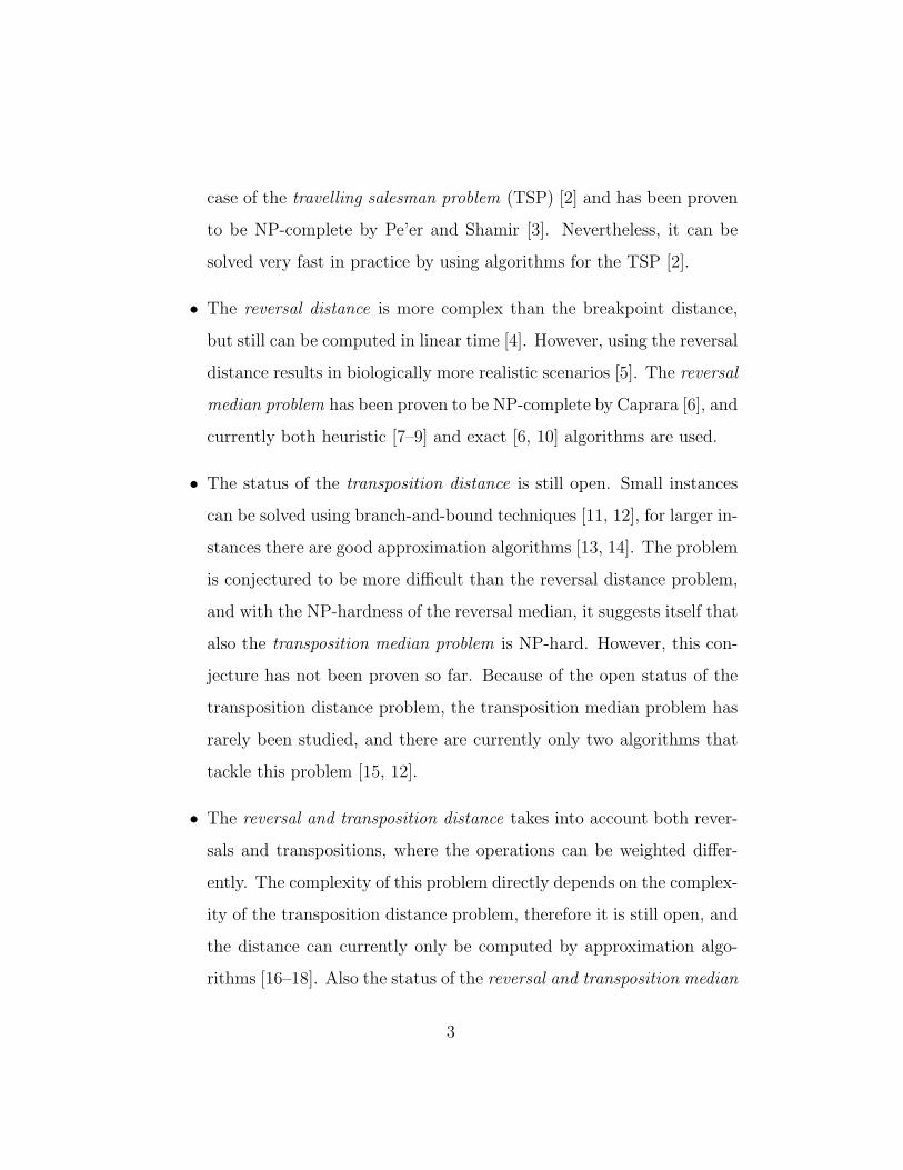
case of the travelling salesman problem (TSP) [2] and has been proven

to be NP-complete by Pe’er and Shamir [3]. Nevertheless, it can be

solved very fast in practice by using algorithms for the TSP [2].

• The reversal distance is more complex than the breakpoint distance,

but still can be computed in linear time [4]. However, using the reversal

distance results in biologically more realistic scenarios [5]. The reversal

median problem has been proven to be NP-complete by Caprara [6], and

currently both heuristic [7–9] and exact [6, 10] algorithms are used.

• The status of the transposition distance is still open. Small instances

can be solved using branch-and-bound techniques [11, 12], for larger in-

stances there are good approximation algorithms [13, 14]. The problem

is conjectured to be more difficult than the reversal distance problem,

and with the NP-hardness of the reversal median, it suggests itself that

also the transposition median problem is NP-hard. However, this con-

jecture has not been proven so far. Because of the open status of the

transposition distance problem, the transposition median problem has

rarely been studied, and there are currently only two algorithms that

tackle this problem [15, 12].

• The reversal and transposition distance takes into account both rever-

sals and transpositions, where the operations can be weighted differ-

ently. The complexity of this problem directly depends on the complex-

ity of the transposition distance problem, therefore it is still open, and

the distance can currently only be computed by approximation algo-

rithms [16–18]. Also the status of the reversal and transposition median

3

problem remains open, and there is currently only one algorithm that

tackles this problem [12].

• To overcome the problems of the reversal and transposition distance,

Yancopoulos et al. [19] introduced the DCJ distance. This distance can

be computed very fast, and also allows to focus on multichromosomal

genomes. Although the DCJ median problem is NP-complete [6, 20],

it has been studied intensively during the last years, resulting in sev-

eral exact and heuristic algorithms that are fast enough for practical

use [21–24].

In this paper, we will prove that the transposition median problem is NP-

complete. The proof is inspired by Caprara’s proof of the NP-completeness of

the reversal median problem. Caprara used a series of reductions, beginning

with the Eulerian cycle decomposition problem (ECD), which has been proven

to be NP-complete by Holyer [25]. As first step, he reduced ECD to the

alternating cycle decomposition problem (ACD) [26]. Then, he reduced ACD

to the cycle median problem (CMP) and finally CMP to the reversal median

problem [6]. Adapting these reductions to the transposition median problem

raises two problems. First, the transposition distance does not depend on

the overall number of cycles in the so-called multiple breakpoint graph, but

on the number of odd cycles, i.e. we have to prove the NP-completeness of

the odd cycle median problem (OCMP). Second, the last reduction requires

us to know whether a permutation is hurdle-free w.r.t. another permutation.

While this is easy to decide for the reversal distance, this is an open problem

for the transposition distance.

The paper is organized as follows. We give the basic definitions and results

4

from the literature in Section 2. In Section 3, we start a series of reductions,

beginning with a modified version of ECD. We will show that OCMP is NP-

complete, and use another reduction to prove the NP-completeness of the

transposition median problem. In Section 4, we discuss the consequences of

this proof for closely related distance measures.

2. Preliminaries

Let π = (π1 . . . πn) be a permutation of {1, . . . , n}. A transposition

t(i, j, k) (with i < j < k) cuts the segment πi . . . πj−1 out of π, and reinserts

it before the element πk, yielding the permutation t(i, j, k)π = (π1 . . . πi−1πj

. . . πk−1πi . . . πj−1πk . . . πn). The transposition distance d(π1, π2) is the min-

imum number of transpositions that is required to transform the permuta-

tion π1 into the permutation π2. The transposition median problem (short

TMP) is defined as follows. Given three permutations π1, π2, and π3, find

a permutation σ such that∑3

i=1 d(σ, πi) is minimized. In order to prove

the NP-hardness of TMP, it is more convenient to write it as a decision

problem. Let π1, π2, and π3 be permutations, and let k be an integer.

Then, (π1, π2, π3, k) ∈ TMP if and only if there is a permutation σ with∑3i=1 d(σ, πi) ≤ k. The proof consists of several polynomial reductions, be-

ginning at the well-known 3SAT problem. More precisely, we will prove that

3SAT ≤p MDECD ≤p OCMP ≤p TMP , where MDECD is the marked

directed Eulerian cycle decomposition problem and OCMP is the odd cycle

median problem. The problem MDECD is defined as follows. Let k be

an integer, and let G = (V,E) be a directed graph where k of its edges

are marked. Then, (G, k) ∈ MDECD if and only if G can be partitioned

5

into edge-disjoint cycles such that each marked edge is in a different cy-

cle. Note that the decomposition may contain cycles that do not contain

a marked edge. This problem is a slight modification of the Eulerian cycle

decomposition problem (short ECD), which has been proven to be NP-hard

by Holyer [25]. The problem OCMP requires the definition of the multiple

breakpoint graph, therefore a mathematical definition of OCMP will be given

after the introduction of this graph in Subsection 2.2.

2.1. Sorting by Transpositions revisited

Before we focus on TMP, we first have to examine the transposition dis-

tance between two permutations π1 and π2 more closely. A key tool for

this is the breakpoint graph, which has been introduced in [27] and can be

constructed as follows. First, write π1 on a straight line. Then, replace

each element π1i by the two nodes vπ1

i tand vπ1

i h, and add the node vb at the

beginning and ve at the end. Note that this gives us an ordering on the

nodes, i.e. we can compare two nodes by the < operator. Now, add red

edges {(vπ1i h, vπ1

i+1t) | 1 ≤ i < n} ∪ {(vb, vπ1

1t), (vπ1

n−1h, ve)}, and black edges

{(vπ2i h, vπ2

i+1t) | 1 ≤ i < n} ∪ {(vb, vπ2

1t), (vπ2

n−1h, ve)} (note that we changed

the coloring of the edges from black/gray in [27] to red/black, because this

corresponds to the colors we use in the multiple breakpoint graph). An exam-

ple of a breakpoint graph is given in Fig. 1. The breakpoint graph naturally

decomposes into cycles of edges with alternating colors. A cycle is called an

l-cycle if it contains l black edges. If l ≥ 3, the cycle is called a long cycle,

otherwise it is called a short cycle. An l-cycle is called an odd cycle if l is

odd, otherwise it is called an even cycle. Let codd(π1, π2) denote the number

of odd cycles in the breakpoint graph of π1 and π2. We say two black edges

6

vb v1t v3t v3h v2t v2h vev1h

Figure 1: The breakpoint graph for π1 = (1 3 2) and π2 = (1 2 3).

(u, v) and (x, y) (with u < v and x < y) intersect if u < x < v < y or

x < u < y < v. Two cycles intersect if they have intersecting black edges.

A transposition on π1 removes three red edges (u, v), (x, y), and (a, b) (with

u < v < x < y < a < b), and replaces them by the red edges (u, y), (a, v),

and (x, b). We say the transposition acts on these edges. A configuration is

a subgraph of a breakpoint graph. If a transposition just acts on edges of

a given configuration, cycles that are not in this configuration remain un-

changed. Thus, configurations are useful to examine the local effect of a

transposition.

Lemma 1. [28] For permutations π1 and π2, the following inequation holds.

n+ 1− codd(π1, π2)

2≤ d(π1, π2) ≤ 1.5

n+ 1− codd(π1, π2)

2

If for two permutations π1 and π2, the transposition distance equals the

lower bound, we say that π1 is hurdle-free w.r.t π2 and vice versa.

Lemma 2. Let π1 and π2 be two permutations. If there is a transposition

t(i, j, k) such that codd(t(i, j, k)π1, π2) − codd(π1, π2) = 2 and t(i, j, k)π1 is

hurdle-free w.r.t. π2, then π1 is hurdle-free w.r.t. π2.

7

Proof.

d(π1, π2) = d(t(i, j, k)π1, π2) + 1

=n+ 1− codd(t(i, j, k)π1, π2)

2+ 1

=n+ 1− codd(π1, π2)

2

Lemma 3. If the breakpoint graph of π1 and π2 contains only short cycles,

then π1 is hurdle-free w.r.t. π2.

Proof. We prove this lemma by induction on the number of 2-cycles in the

breakpoint graph. If it contains only 1-cycles, then d(π1, π2) = 0, and π1 is

clearly hurdle-free w.r.t. π2. Otherwise, according to [27], there are two con-

secutive transpositions that transform two 2-cycles into four 1-cycles (note

that the number of even cycles is always even, see [11]), i.e. both transposi-

tions increase the number of odd cycles by 2. As the resulting permutation

is hurdle-free by induction hypothesis, the proposition follows by applying

Lemma 2 twice.

Lemma 4. If a breakpoint graph contains red edges (u, v), (x, y), (a, b) (with

u < v, x < y, and a < b) and intersecting black edges (u, y), (x, b), then a

transposition acting on these red edges splits an l-cycle into an (l − 2)-cycle

and two 1-cycles with edges (u, y) and (x, b).

Proof. As the black edges are intersecting, the ordering of the nodes must be

u < v < x < y < a < b or a < b < u < v < x < y or x < y < a < b < u < v.

In all cases, the transposition creates red edges (u, y), (x, b), and (a, v). The

8

u v x y a b u by a v x

Figure 2: The effect of the transposition described in Lemma 4. The dashed line is a path

of alternating black and red edges. The operation splits the two 1-cycles with edges (u, y)

and (x, b) from an l-cycle.

black edges remain unchanged, thus the two 1-cycles with edges (u, y) and

(x, b) are split from the l-cycle. For an illustration, see Fig. 2

2.2. Multiple breakpoint graphs

The key tool to examine TMP is the multiple breakpoint graph (short

MB graph), due to [6]. Before defining the MB graph, we first need some

definitions. Given a set of nodes V = {vb, v1t, v1h, v2t, v2h, . . . , vnt, vnh, ve}, a

perfect matching M is a set of edges such that each node in V is endpoint of

exactly one edge in M . The perfect matching associated with a permutation

π is defined by

M(π) = {(vb, vπ1t), (vπnh, ve)} ∪ {(vπih, vπi+1t) | 1 ≤ i < n}

If a perfect matching M is associated with a permutation, i.e. M = M(σ)

for a permutation σ, then M is called a permutation matching. Given

permutations π1, . . . , πq, the MB graph G(π1, . . . , πq) = (V,E) is an edge

colored multigraph (i.e. it can contain parallel edges with common end-

points) with node set V = {vb, v1t, v1h, v2t, v2h, . . . , vnt, vnh, ve} and edge set

E = M(π1)∪ · · · ∪M(πq), where the edges of M(πi) have the color i. In the

9

vb ve

v2h

v1t

v1h

v2t

v3t

v3h

Figure 3: The MB graph for π1 = (1 2 3), π2 = (1 3 2), and π3 = (3 2 1). The graph

contains 2 odd red/green cycles, 2 odd green/blue cycles, and 2 even red/blue cycles.

following, let color 1 be red, let color 2 be green, and let color 3 be blue. For

an example, see Fig. 3. The edges of two perfect matchings M(πi),M(πj) de-

compose the MB graph into cycles, corresponding to the cycles in the break-

point graph of πi and πj. The odd cycle median problem (short OCMP) is

defined as follows. Let π1, π2, π3 be permutations of {1, . . . , n}, and let k be

an integer. Then, (π1, π2, π3, k) ∈ OCMP if and only if there is a permuta-

tion σ with∑3

i=1 codd(σ, πi) ≥ k . Solving an OCMP instance is equivalent

to finding a permutation matching M(σ) such that∑3

i=1 codd(σ, πi) is maxi-

mized. This sum is also called the solution value of M(σ). In the following,

let the edges of every permutation matching we examine be black.

We will now examine which conditions a graph has to fulfill to be a valid MB

graph.

Lemma 5. Let V t and V h be two disjoint node sets, and let G′ = (V t ∪

V h,M1 ∪M2 ∪ . . .M q) be an edge-colored graph, where each M i is a perfect

matching, each edge in M i has color i, and each edge connects a node in V t

with a node in V h. Furthermore, let H be a perfect matching such that each

edge in H connects a node in V t with a node in V h, and H ∪M i defines

10

a Hamiltonian cycle of V t ∪ V h (i.e. a cycle that visits every node in the

graph) for 1 ≤ i ≤ q. Then, there exist permutations π1, . . . , πq such that G′

is isomorphic to the MB graph G(π1, . . . , πq).

Proof. We will give a constructive proof on how to create the permutations

π1, . . . , πq such thatG′ is isomorphic to the MB graphG(π1, . . . , πq). For this,

set n = |V t|−1. Now, arbitrarily label the nodes in V t with v1t, v2t, . . . , vnt, vb.

Label the nodes in V h such that H = {(vit, vih) | 1 ≤ i ≤ n}∪ {(vb, ve)}. Let

vb, vj1t, vj1h, vj2t, . . . , vjnh, ve, vb be the Hamiltonian cycle defined by H ∪M j.

Then, set πj = (j1 . . . jn). It is clear to see that πj is a valid permutation,

and the perfect matching associated with πj is M j. Therefore, with the given

node labeling, G(π1, . . . , πq) = G′.

In the following, such a matching H is called a base matching of the

graph. For a closer examination whether a base matching exists, we need

another important notion, introduced in [6]. Given a perfect matching M

on a node set V and an edge e = (u, v), M/e is defined as follows. If

e ∈ M,M/e = M \ {e}. Otherwise, letting (a, u), (b, v) be the two edges in

M incident to u and v, M/e = M \ {(a, u), (b, v)} ∪ {e}.

Lemma 6. [6] Given two perfect matchings M,L of V and an edge e =

(u, v) ∈ M with e 6∈ L, M ∪ L defines a Hamiltonian cycle of V if and only

if (M/e) ∪ (L/e) defines a Hamiltonian cycle of V \ {u, v}.

Given an MB graph G = (V,M(π1)∪ · · · ∪M(πq)), the contraction of an

edge e = (u, v) yields the graph G/e = (V \{u, v},M(π1)/e∪· · ·∪M(πq)/e).

For an example, see Fig. 4.

11

vb ve

v2h

v1t

v1h

v2t

v3t

v3h

vb

v2h

v1t

v1h

v2t

v3t

Figure 4: The contraction of the edge (v3h, ve) in the left graph (dotted edge) yields the

right graph.

Lemma 7. Let V t and V h be two disjoint node sets, and let G = (V =

V t ∪ V h,M1 ∪M2) be an edge-colored graph, where M1 (M2) is a perfect

matching with red (green) edges, and each edge connects a node in V t with a

node in V h. If M1 ∪M2 define an even number of even cycles on V , then G

has a base matching H.

Proof. We prove this lemma by an induction on the size of V t. If |V t| = 1,

then the graph consists of just one parallel red and green edge, and there

trivially exists a base matching H satisfying the conditions of Lemma 5, i.e.

both H ∪M1 and H ∪M2 define a Hamiltonian cycle on V . For |V t| > 1,

we must distinguish two cases. If M1 ∪M2 defines at least two cycles on

V , then there are nodes u ∈ V t and v ∈ V h such that these nodes are in

different cycles. The contraction of e = (u, v) merges these two cycles, and

the resulting cycle is even if and only if exactly one of the merged cycles

was even. In other words, the contraction of e reduces |V t| by 1 and does

not change the parity of the number of even cycles. Due to the induction

hypothesis, G/e has a base matching H. According to Lemma 6, H ∪ {e}

is a base matching of G. The case where M1 ∪M2 defines just one cycle

12

can be proven similarly. This cycle must be odd, and has at least length 3.

Therefore, there are nodes u, v such that the edge e = (u, v) is neither in M1

nor in M2. The contraction of e splits the cycle, and again the parity of the

number of even cycles cannot be changed. With the same argumentation as

above, it follows that a base matching H of G/e can be extended to a base

matching H ∪ {e} of G.

3. The Complexity of OCMP and TMP

In this section, we will use a series of reductions to show that both OCMP

and TMP are NP-hard. The proof that both problems are in NP is trivial,

thus it directly follows that both problems are NP-complete. The starting

problem in our hardness proofs is MDECD, which is a small modification of

ECD.

Theorem 1. [25] ECD is NP-hard.

Lemma 8. MDECD is NP-hard.

Proof. By following the proof for ECD in [25] and simply directing the edges

in the graph construction, one can prove that partitioning a directed graph

into edge-disjoint cycles of length 3 is NP-hard (see also [29]). Furthermore,

the edges of the graph can be partitioned into 3 groups such that each cycle

of length 3 must contain one edge of each group. While Holyer used this fact

to extend his proof to cycles of arbitrary length, we mark all edges of one

group, i.e. each possible cycle of length 3 contains exactly one marked cycle.

This completes the proof for k = |E|/3.

13

In the following, we will assume that that for an MDECD instance, each

node has the same in- and out-degree.

3.1. Reduction from MDECD to OCMP

In order to prove the NP-hardness of OCMP, we first have to show

that MDECD is NP-hard even when the in- and out-degree of all nodes

is bounded by 2. Next, we provide a transformation from a directed graph

G with bounded degree to an MB graph G′(π1, π2, π3) such that (G, k) ∈

MDECD ⇔ (π1, π2, π3, f(G, k)) ∈ OCMP (where f(G, k) is a function

that can be evaluated in polynomial time).

A permutation network is a directed graph Yd where 2d of the nodes are

labelled by i1, . . . , id, o1, . . . , od (the input and output nodes). Furthermore,

for each permutation ρ ∈ Σd, there are edge-disjoint paths p1, . . . , pd in Yd

such that path pj goes from ij to oρ(j).

Lemma 9. [30] For each d, a permutation network Yd of size O(d log d) can

be constructed in polynomial time. Furthermore, for each node v in Yd, the

following proposition holds.

• degin(v) ≤ degout(v) ≤ 2 if v is an input node.

• degout(v) ≤ degin(v) ≤ 2 if v is an output node.

• degin(v) = degout(v) ≤ 2 if v is an inner node.

By adding edges from the output nodes to the input nodes, it is possible

to obtain a permutation network Y ′d where degout(i) − degin(i) = 1 for all

input nodes i, and degin(o)− degout(o) = 1 for all output nodes o.

Let G be a directed graph with k marked edges. We obtain the graph G by

14

a

b

c

d

e

f

g

h

Y ′4

Y4

a

b

c

d

e

f

g

h

Figure 5: Transformation of a node v with degree 8 into a Y ′4 .

replacing each node v in G with degree d > 4 by a Y ′d/2. The incoming edges

in v are arbitrarily connected to the input nodes of the corresponding Yd/2,

and the outgoing edges in v are connected to its output nodes (see Fig. 5).

Note that in G, all nodes v satisfy degin(v) = degout(v) ≤ 2.

Lemma 10. (G, k) ∈MDECD if and only if (G, k) ∈MDECD.

Proof. If (G, k) ∈ MDECD, we can map the cycles in G to cycles in G

by adding the corresponding paths through the permutation network for

each node in a cycle. As the paths through the permutation network are

edge-disjoint, the cycles in G also are edge-disjoint. Because all nodes v

satisfy degin(v) = degout(v), the remaining edges in the permutation network

can be partitioned into edge-disjoint cycles. Thus, G can be partitioned

into edge-disjoint cycles and each marked edge is in a different cycle, i.e.

(G, k) ∈ MDECD. On the other hand, if (G, k) ∈ MDECD, then we can

remove the paths in the permutation networks from each cycle to obtain a

cycle decomposition of G, i.e. (G, k) ∈MDECD.

The transformation from G to G can be computed in polynomial time,

15

i.e., the construction of G describes a polynomial reduction from MDECD

to MDECD with bounded node degrees.

Theorem 2. MDECD is NP-hard even when the degree of all nodes is

bounded by 4. Furthermore, the claim still holds for graphs where |V |+|E|−k

is odd.

Proof. The first proposition directly follows from Lemmas 9 and 10. Now,

assume that our transformation resulted in a graph G = (V,E) where |V |+

|E| − k is even. We further transform G into G = (V , E) as follows (see

also Fig. 6). Let v1 and v2 be two nodes of degree 2 that are not connected

by an edge (if no such nodes exist, they can be created by splitting a non-

marked edge without changing the parity of |V | + |E| − k). Create a new

node vx and set V = V ∪ {vx}, E = E ∪ {(v1, v2), (v2, vx), (vx, v1)}, where

(vx, v1) is a marked edge. As we added a cycle with one marked edge, it is

clear to see that if (G, k) ∈ MDECD, then (G, k + 1) ∈ MDECD . On

the other hand, each cycle decomposition of G can be modified such that the

added edges form one cycle. This leads to a cycle decomposition of G, i.e.

(G, k + 1) ∈ MDECD implies (G, k) ∈ MDECD. Together with the fact

that |V |+ |E| − (k + 1) is odd, the second proposition follows.

Now, let G = (V,E) be a directed graph with k marked edges, degin(v) =

degout(v) ≤ 2 ∀v ∈ V , and |V | + |E| − k odd. Let V2 be the nodes with

deg(v) = 2, and let V4 be the nodes with deg(v) = 4. Let E be an Eulerian

cycle in G (which clearly exists and can be computed in polynomial time).

We will now describe a polynomial transformation from G to an MB graph

G′ = (V ′, E ′) (for a graphical representation, see Fig. 7).

16

v2

v1

v2

vxv1

G G

Figure 6: Transformation of G = (V,E) into G = (V , E), such that |V |+ |E| − k is odd.

Marked edges are dashed.

1. For each node v ∈ V2, G′ contains a subgraph W2 with node set

{v−, v+}, and a parallel red and green edge (v−, v+). The node v−

is called the input node of the W2, and v+ is called the output node.

2. For each node v ∈ V4, G′ contains a subgraph W4 with node set

{v1−, v1+, . . . , v4−, v4+}, red edges {(v1−, v3+), (v2−, v2+), (v3−, v1+), (v4−, v4+)},

green edges {(v1−, v2+), (v2−, v1+), (v3−, v3+), (v4−, v4+)}, and blue edges

{(v3−, v4+), (v4−, v3+)}. The nodes v1− and v2− are called the input

nodes of the W4, and v1+ and v2+ are called the output nodes.

3. For each marked edge (v, w) ∈ E, there is a blue edge (v′, w′) in G′

which connects the corresponding subgraphs of v and w. v′ is always

an output node of the corresponding subgraph, and w′ is an input node

of the corresponding subgraph.

4. For each non-marked edge (v, w) ∈ E, G′ contains two nodes v−, v+,

a parallel red and green edge (v−, v+), and two blue edges (v′, v−) and

(v+, w′), where v′ is an output node of the subgraph corresponding to

v, and w′ is an input node of the subgraph corresponding to w.

5. The endpoints of a blue edge are always chosen such that each node is

17

v+

v4+

v− v4−

v1+

v1− v2−

v2+v′

u′

(b)(a) (c)

v3+

v3− v+

v−

Figure 7: Transformation steps from a Graph G to an MB graph G′. (a) a W2 (b) a W4

(c) transformation of a non-marked edge.

incident to exactly one blue edge. Furthermore, if v ∈ V4 and E contains

two consecutive edges (u, v), (v, w), the corresponding blue edges are

either of the form (u′, v1−), (v2+, w′) or (u′, v2−), (v1+, w

′). Thus, the

Eulerian cycle E is transformed into a cycle of alternating green and

blue edges that passes each V2 and V4. This cycle contains one green

edge for each V2, for each V4, and for each non-marked edge.

Lemma 11. G′ is an MB graph, and a base matching H can be calculated

in polynomial time.

Proof. The node set V ′ can be divided into V − and V + such that V − contains

all nodes v−, v1−, v2−, v3−, v4−, and V + contains all nodes v+, v1+, v2+, v3+, v4+.

Thus, all red, green, and blue edges connect a node in V − with a node in V +.

According to Lemma 5, it remains to show that there is a base matching H.

This base matching can be built iteratively as follows. For each W4 in G′, we

add the edges (v2−, v3+), (v3−, v2+), and (v4−, v1+) to H. Then, we contract

18

these edges. Let (u, v1−), (v, v2−), (w, v1+), (x, v2+) be the incoming/outgoing

blue edges of a W4. Then, after the contraction, we have the blue edges

(u, v1−), (x, v4+), (v, w) and a parallel red and green edge (v1−, v4+). If we

would now merge v1− and v4+, we would restore the Eulerian cycle E . There-

fore, we have now an Eulerian cycle of alternating blue and red/green edges.

This cycle contains one green edge for each V2, for each V4, and for each non-

marked edge. This is equivalent to the number of vertices plus the number

of non-marked edges in G. Because we assumed that in G, |V | + |E| − k

is odd, this cycle is also odd. Therefore, the preconditions of Lemma 7 are

fulfilled, and we can continue with the algorithm devised there.

Lemma 12. Let G′ be an MB graph with base matching H that has been

constructed as described above. Then, every perfect matching M containing

only edges parallel to red and green edges is a permutation matching.

Proof. If we divide V ′ into V − and V + as described above, every edge of M

connects a node in V − with a node in V +. For every W4 in the MBG, M must

be parallel either to all green edges or to all red edges. After contracting all

edges of H in each W4, the set of red and green edges and M are identical.

Because the red and green edges are permutation matchings, M must also

be a permutation matching.

We call a perfect matching canonical if, whenever there is a parallel red and

green edge, these edges are also parallel to an edge in M .

Lemma 13. Given a permutation matching M(σ) on G′, it is always possible

to find a canonical matching whose solution value is at least as good.

19

Proof. Let M be a perfect matching, and let v and w be two nodes that

are connected by a red and a green edge, but not by a black edge. Assume

that there are black edges (x, v) and (y, w). We replace these edges with the

black edges (x, y) and (u, v). This splits both a red/black and a green/black

cycle, but may merge two blue/black cycles. If the red/black cycle or the

green/black cycle was an even cycle, or we did not merge two odd blue/black

cycles, the number of odd cycles is not decreased. Otherwise, the number of

odd cycles is decreased by 2, and the red/black, green/black, and blue/black

cycle containing the black edge (x, y) are even cycles. Therefore, exchanging

the endpoints of (x, y) with those of another black edge cannot remove any

further odd cycles. However, such an exchange is possible such that the

red/black cycle is split into two odd cycles, i.e. this operation increases the

number of odd cycles by at least 2. Both operations together do not decrease

the overall number of odd cycles. These steps can be repeated until M is a

canonical matching.

Lemma 14. A canonical matching has at most k odd blue/black cycles.

Proof. By construction, G′ contains pairs of blue edges that are separated

by a parallel red and green edge. These pairs contain all blue edges, except

those that correspond to a marked edge in G. Thus, every odd blue/black

cycle must contain at least one blue edge corresponding to a marked edge

in G. As there are only k marked edges in G, there can be at most k odd

blue/black cycles if the black edges are a canonical matching.

Lemma 15. For every perfect matching, the sum of the number of red/black

and green/black odd cycles is ≤ 2|V2|+ 6|V4|+ 2|E| − 2k. The equality holds

if and only if all black edges are parallel to a red or green edge.

20

Proof. If e is a black edge in a red/black kr-cycle, then let the red score of e

be 1/kr if kr is odd, 0 otherwise. The green score is defined analogously for

green/black cycles. The score of a black edge is the sum of its red and green

score. Clearly, the number of red/black and green/black odd cycles is the sum

of the scores of all black edges. If a red edge, a green edge, and a black edge

are parallel, then the score of the black edge is 2, which maximizes this value.

This score can be achieved by at most |V2|+|V4|+|E|−k black edges, because

this is the number of parallel red and green edges. The second best possible

score is 4/3, and it is achieved if and only if a black edge is in a red/black 1-

cycle and a green/black 3-cycle or vice versa. If all edges in a perfect matching

are parallel to a red or green edge, the black edges in each W4 are parallel to

edges of the same color, forming four 1-cycles with this color and a 1-cycle

and a 3-cycle with the edges of the other color. Thus, the number of black

edges with score 2 is maximized, all other black edges have score 4/3, leading

to an overall score of 2 ·#W2 + 2 ·#W4 + 2 ·#non-marked edges + 4 ·#W4 =

2|V2|+6|V4|+2|E|−2k. If the matching contains a black edge that is neither

parallel to a red nor to a green edge, then the score of this edge is < 4/3,

and the sum of all scores can no longer be maximal.

Theorem 3. There is a permutation matching M(σ) with∑3

i=1 codd(σ, πi) =

2|V2|+ 6|V4|+ 2|E| − k if and only if (G, k) ∈MDECD.

Proof. According to Lemma 13, it is sufficient to consider canonical match-

ings. Together with Lemmas 14 and 15, it follows that the maximum number

of cycles is 2|V2| + 6|V4| + 2|E| − k, and this can only be achieved if each

black edge is parallel to a red or green edge. Then, all black edges in one W4

must be parallel to edges of the same color. Depending on whether they are

21

parallel to the red or the green edges, we get blue/black paths from v1− to v1+

and from v2− to v2+, or from v1− to v2+ and from v2− to v1+. Thus, there is

a one-to-one correspondence between black/blue cycles in G′ and cycles in G

(except for possible even black/blue cycles that are completely within a W4).

A black/blue cycle in G′ is odd if the corresponding cycle in G contains an

odd number of marked edges. Therefore, if there is a permutation matching

M(σ) with∑3

i=1 codd(σ, πi) = 2|V2|+ 6|V4|+ 2|E| − k, it defines k blue/black

odd cycles. These cycles describe the partitioning of G into k edge-disjoint

cycles such that each cycle contains a marked edge, i.e. (G, k) ∈ MDECD.

On the other hand, such a partitioning of G can be used to obtain a permu-

tation matching M(σ) with∑3

i=1 codd(σ, πi) = 2|V2|+ 6|V4|+ 2|E| − k.

Corollary 1. OCMP is NP-complete.

3.2. Reduction from OCMP to TMP

To prove the NP-hardness of TMP, we describe a transformation from

an MB graph G(π1, π2, π3) into an MB graph G(π1, π2, π3), such that every

permutation σ that minimizes∑3

i=1 d(σ, πi) also maximizes∑3

i=1 codd(σ, πi).

Let G(π1, π2, π3) = (V,M(π1) ∪M(π2) ∪M(π3)) be an arbitrary MB graph

with base matching H, and let M(σ) be a canonical matching that maximizes∑3i=1 codd(σ, π

i). First, we will modify the MB graph such that σ is hurdle-

free w.r.t. π1. Although we do not know M(σ), we can presume that some

edges of M(σ) are given due to the fact that it is a canonical matching. With

these edges, we already get some red/black cycles and paths. Thus, there

are red edges that are certainly not in a long red/black cycle. Let (u, v) be a

red edge that might be in a long red/black cycle, and let (x, u), (v, y) be the

22

a bx c v g h yd e f u

x u v y

Figure 8: Transformation of a subgraph of G containing a red edge that might belong to

a long red/black cycle.

adjacent edges of the base matching H. We transform the MB graph into

an MB graph G(π1, π2, π3) = (V , M1 ∪ M2 ∪ M3) with base matching H as

follows (for a graphical representation, see Fig. 8).

1. V = V ∪ {a, b, c, d, e, f, g, h}.

2. H = H \ {(x, u), (v, y)} ∪ {(x, a), (b, c), (d, e), (f, u), (v, g), (h, y)}

3. M1 = M(π1) ∪ {(a, b), (c, d), (e, f), (g, h)}

4. Add green and blue edges (a, f), (b, e), (c, h), and (d, g), i.e.

M2 = M(π2) ∪ {(a, f), (b, e), (c, h), (d, g)} and

M3 = M(π3) ∪ {(a, f), (b, e), (c, h), (d, g)}.

Lemma 16. If G(π1, π2, π3) is a valid MB graph, then G(π1, π2, π3) is also

a valid MB graph.

Proof. Let V t and V h be two disjoint node sets with V = V t ∪ V h such that

every edge in M(π1) ∪M(π2) ∪M(π3) ∪ H connects a node in V t with a

node in V h. W.l.o.g, assume that u ∈ V t. If we set V t = V t ∪ {a, c, e, g}

and V h = V h ∪ {b, d, f, h}, then every edge in M1 ∪ M2 ∪ M3 ∪ H connects

23

a node in V t with a node in V h. If we contract the red edges (a, b), (c, d),

(e, f), (g, h), we get the Hamiltonian cycle M(π1) ∪ H on V . According to

Lemma 6, M1 ∪ H defines a Hamiltonian cycle on V . The proof that also

M2 ∪ H and M3 ∪ H define Hamiltonian cycles on V is analogous, but with

contracting the edges (a, f), (b, e), (c, h), (d, g). Thus, all preconditions of

Lemma 5 are fulfilled, and G(π1, π2, π3) is a valid MB graph.

Lemma 17. There is a one-to-one correspondence between canonical match-

ings M(σ) of G(π1, π2, π3) with∑3

i=1 codd(σ, πi) = k and canonical matchings

M(σ) of G(π1, π2, π3) with∑3

i=1 codd(σ, πi) = k + 8.

Proof. M(σ) must contain the edges (a, f), (b, e), (c, h), and (d, g) because it

is canonical. These edges define 2 red/black 2-cycles, 4 green/black 1-cycles,

and 4 blue/black 1-cycles (overall 8 odd and 2 even cycles). If we remove these

cycles from G(π1, π2, π3), the remaining graph is equivalent to G, thus each

canonical matching M(σ) of G(π1, π2, π3) with∑3

i=1 codd(σ, πi) = k corre-

sponds to a canonical matching M(σ) of G(π1, π2, π3) with∑3

i=1 codd(σ, πi) =

k + 8.

Lemma 18. If σ is hurdle-free w.r.t. π2, then the corresponding permutation

σ is also hurdle-free w.r.t. π2.

Proof. If one compares the breakpoint graph of σ and π2 with the one of σ

and π2, one can see that the transformation just added 4 1-cycles without

changing the structure of any other cycle. Thus, for each sorting sequence

that sorts σ into π2, there is an equivalent sorting sequence from σ to π2.

Of course, this lemma also holds for π3. To make σ hurdle-free w.r.t. π1, we

repeat the transformation step for every red edge that might belong to a a

24

red/black l-cycle with l ≥ 3. Let the resulting graph be G(π1, π2, π3).

Lemma 19. Let M(σ) be a canonical matching of G(π1, π2, π3). Then, σ is

hurdle-free w.r.t. π1.

Proof. Due to the construction rules, the following condition holds for the

breakpoint graph of σ and π1. For each red edge e that belongs to a long cycle,

the adjacent black edges intersect with the black edges of a 2-cycle c. We call

c the companion of e. The black edges of c neither intersect with any other

black edges of a long cycles nor with black edges of another companion. The

configuration of an edge with its companion is illustrated in Fig. 9. We will

now describe a sequence of transpositions that sorts σ into π1 such that each

transposition increases the number of odd cycles by 2. We start the sorting

with an arbitrary red edge e of a long cycle. If the black edges adjacent to

e intersect, we apply the transposition described in Lemma 4. This might

destroy the companion of e, i.e. the intersection condition of the companion

is no longer fulfilled. However, all other red edges in a long cycle still have

a valid companion. Now, assume that the black edges adjacent to e do not

intersect. Let f and g be the red edges connected to e by a black edge.

Fig. 10 describes a sequence of 3 transpositions where each transposition

increases the number of odd cycles by 2. The sequence uses the companions

of f and g. Note that the sequence also works if the black edges adjacent

to f or g intersect. After the sequence, all edges in a long cycle expect e

still have a companion. Thus, we can repeat this step (always starting with

edge e) until e is in a short cycle, and then continue with another long cycle.

When no long cycle remains, the resulting permutation is hurdle-free due to

Lemma 3.

25

cc′

e

Figure 9: The configuration of the companion c of a red edge e. The black edges adjacent

to e may also intersect. By construction, c intersects with another 2-cycle c′. However, c′

is not a companion of a red edge.

We continue the transformation by performing equivalent steps for green

and blue edges. Let G(π1, π2, π3) be the resulting MB graph, and let σ be a

canonical matching on this graph. Clearly, σ is hurdle-free w.r.t. π1, π2, and

π3.

Theorem 4. Let π1, π2, π3 be permutations of size n, and let G(π1, π2, π3) be

their MB graph. Let G(π1, π2, π3) be the breakpoint graph obtained by trans-

forming G(π1, π2, π3), and let m be the number of performed steps during the

transformation. Then, (π1, π2, π3, k) ∈ OCMP if and only if (π1, π2, π3, 3(n+1)+4m−k2

) ∈

TMP .

Proof. As we have shown in Lemma 17, (π1, π2, π3, k) ∈ OCMP if and

only if (π1, π2, π3, k + 8m) ∈ OCMP . The size of the permutations π1,

π2, and π3 is n + 4m. Assume there is a permutation matching M(σ) with∑3i=1 codd(σ, π

i) ≥ k + 8m. W.l.o.g. M(σ) is a canonical matching, and due

to Lemma 19, we can assume that σ is hurdle-free w.r.t. π1, π2, and π3.

26

f g

ef g

e

Figure 10: A sequence of 3 transpositions that can be applied when the black edges

adjacent to e do not intersect. The 2-cycles belong to the companions of f and g. The

dashed line is a path of alternating black and red edges. The vertical black lines indicate

the red edges where the next transposition acts on. Note that the sequence also works if

the black edges adjacent to f or g intersect.

27

Thus,

3∑i=1

d(σ, πi) =3∑i=1

n+ 4m+ 1− codd(σ, πi)2

=3(n+ 1) + 12m−

∑3i=1 codd(σ, π

i)

2

≤ 3(n+ 1) + 4m− k2

.

On the other hand, let there be a permutation σ with∑3

i=1 d(σ, πi) ≤3(n+1)+4m−k

2. Then, we get (with Lemma 1)

3∑i=1

n+ 4m+ 1− codd(σ, πi)2

=3(n+ 1) + 12m−

∑3i=1 codd(σ, π

i)

2

≤3∑i=1

d(σ, πi)

≤ 3(n+ 1) + 4m− k2

,

and therefore3∑i=1

codd(σ, πi) ≥ k + 8m.

In other words, (π1, π2, π3, k+8m) ∈ OCMP if and only if (π1, π2, π3, 3(n+1)+4m−k2

) ∈

TMP .

Corollary 2. TMP is NP-complete.

4. Conclusion

In this paper, we have proven that TMP is NP-complete. As a direct con-

sequence, also the reversal and transposition median problem is NP-complete

if both operations are weighted equally. For a weight ratio of reversals :

28

transpositions = 1 : 2, the NP-completeness directly follows from [6]. For

all weight ratios in between, the complexity is still open. Another closely

related problem is the transposition median problem on the symmetric group

Sn (short TMS), which has been extensively studied by Eriksen [31, 32]

(note that in this problem, transpositions are defined different than in our

problem). Although this problem is closely related to the DCJ median prob-

lem, its NP-hardness could not be proven so far, mainly because one has to

deal with directed graphs [32]. As our proof extends some steps of Caprara’s

proof to directed graphs, we hope that it can also give us new insights about

TMS.

[1] P. Pevzner, G. Tesler, Human and mouse genomic sequences reveal ex-

tensive breakpoint reuse in mammalian evolution, Proceedings of the

National Academy of Sciences 100 (13) (2003) 7672–7677.

[2] D. Sankoff, M. Blanchette, Multiple genome rearrangement and break-

point phylogeny, Journal of Computational Biology 5 (3) (1998) 555–

570.

[3] I. Pe’er, R. Shamir, The median problems for breakpoints are NP-

complete, Tech. Rep. TR98-071, Electronic Colloquium on Computa-

tional Complexity (1998).

[4] D. Bader, B. Moret, M. Yan, A linear-time algorithm for computing

inversion distance between signed permutations with an experimental

study, Journal of Computational Biology 8 (2001) 483–491.

[5] B. Moret, A. Siepel, J. Tang, T. Liu, Inversion medians outperform

29

breakpoint medians in phylogeny reconstruction from gene-order data,

in: Proc. 2nd Workshop on Algorithms in Bioinformatics, Vol. 2452 of

Lecture Notes in Computer Science, Springer-Verlag, 2002, pp. 521–536.

[6] A. Caprara, The reversal median problem, INFORMS Journal on Com-

puting 15 (1) (2003) 93–113.

[7] B. Bourque, P. Pevzner, Genome-scale evolution: Reconstructing gene

orders in the ancestral species, Genome Research 12 (1) (2002) 26–36.

[8] W. Arndt, J. Tang, Improving inversion median computation using com-

muting reversals and cycle information, in: Proc. 5th Annual RECOMB

Satellite Workshop on Comparative Genomics, Vol. 4751 of Lecture

Notes in Computer Science, Springer-Verlag, 2007, pp. 30–44.

[9] K. Swenson, Y. To, J. Tang, B. Moret, Maximum independent sets of

commuting and noninterfering inversions, BMC Bioinformatics 10(Suppl

1) (2009) S6.

[10] A. Siepel, B. Moret, Finding an optimal inversion median: Experimental

results, in: Proc. 1st Workshop on Algorithms, Vol. 2149 of Lecture

Notes in Computer Science, Springer-Verlag, 2001, pp. 189–203.

[11] D. Christie, Genome rearrangement problems, Ph.D. thesis, University

of Glasgow (1998).

[12] M. Bader, On reversal and transposition medians, Proceedings of World

Academy of Science, Engineering and Technology 54 (2009) 667–675.

30

[13] T. Hartman, R. Shamir, A simpler and faster 1.5-approximation al-

gorithm for sorting by transpositions, Information and Computation

204 (2) (2006) 275–290.

[14] I. Elias, T. Hartman, A 1.375-approximation algorithm for sorting by

transpositions, IEEE/ACM Transactions on Computational Biology and

Bioinformatics 3 (4) (2006) 369–379.

[15] F. Yue, M. Zhang, J. Tang, A heuristic for phylogenetic reconstruction

using transposition, in: Proc. 7th IEEE Conference on Bioinformatics

and Bioengineering, 2007, pp. 802–808.

[16] T. Hartman, R. Sharan, A 1.5-approximation algorithm for sorting by

transpositions and transreversals, Journal of Computer and System Sci-

ences 70 (3) (2005) 300–320.

[17] N. Eriksen, (1 + ε)-approximation of sorting by reversals and transposi-

tions, Theoretical Computer Science 289 (1) (2002) 517–529.

[18] M. Bader, E. Ohlebusch, Sorting by weighted reversals, transpositions,

and inverted transpositions, Journal of Computational Biology 14 (5)

(2007) 615–636.

[19] S. Yancopoulos, O. Attie, R. Friedberg, Efficient sorting of genomic

permutations by translocation, inversion and block interchange, Bioin-

formatics 21 (16) (2005) 3340–3346.

[20] E. Tannier, C. Zheng, D. Sankoff, Multichromosomal genome median

and halving problems, in: Proc. 8th Workshop on Algorithms in Bioin-

31

formatics, Vol. 5251 of Lecture Notes in Computer Science, Springer-

Verlag, 2008, pp. 1–13.

[21] Z. Adam, D. Sankoff, The ABCs of MGR with DCJ, Evolutionary Bioin-

formatics 4 (2008) 69–74.

[22] A. Xu, A fast and exact algorithm for the median of three problem

- a graph decomposition approach, Journal of Computational Biology

16 (10) (2009) 1369–1381.

[23] A. Xu, DCJ median problems on linear multichromosomal genomes:

Graph representation and fast exact solutions, in: Proc. 7th Annual

RECOMB Satellite Workshop on Comparative Genomics, Vol. 5817 of

Lecture Notes in Bioinformatics, Springer-Verlag, 2009, pp. 70–83.

[24] M. Zhang, W. Arndt, J. Tang, An exact solver for the DCJ median

problem, in: Proc. 14th Pacific Symposium on Biocomputing, World

Scientific, 2009, pp. 138–149.

[25] I. Holyer, The NP-completeness of some edge-partition problems, SIAM

Journal on Computing 10 (4) (1981) 713–717.

[26] A. Caprara, Sorting permutations by reversals and Eulerian cycle de-

compositions, SIAM Journal on Discrete Mathematics 12 (1999) 91–110.

[27] V. Bafna, P. Pevzner, Genome rearrangements and sorting by reversals,

SIAM Journal on Computing 25 (2) (1996) 272–289.

[28] V. Bafna, P. Pevzner, Sorting by transpositions, SIAM Journal on Dis-

crete Mathematics 11 (2) (1998) 224–240.

32

[29] A. Amir, T. Hartman, O. Kapah, A. Levy, E. Porat, On the cost of inter-

change rearrangement in strings, in: Proc. 15th Annual European Sym-

posium on Algorithms, Lecture Notes in Computer Science, Springer-

Verlag, 2007, pp. 99–110.

[30] A. Waksman, A permutation network, Journal of the ACM 15 (1) (1968)

159–163.

[31] N. Eriksen, Reversal and transposition medians, Theoretical Computer

Science 374 (2007) 111–126.

[32] N. Eriksen, Median clouds and a fast transposition median solver,

unpublished results.

URL http://www.math.chalmers.se/∼ner/artiklar/EriksenFPSAC2009.pdf

33