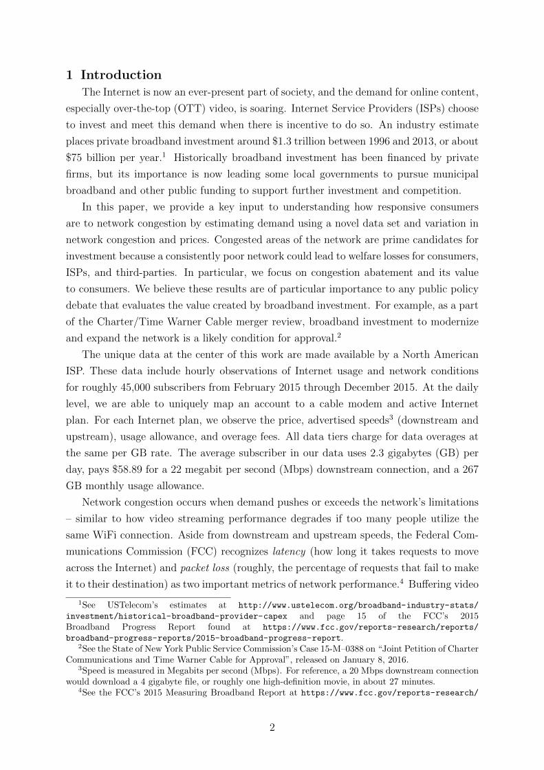
The Tragedy of the Last Mile: CongestionExternalities in Broadband Networks∗

Jacob B. Malone† Aviv Nevo‡ Jonathan W. Williams§

PRELIMINARY AND INCOMPLETE: April 2016

Abstract

We flexibly estimate demand for residential broadband accounting for congestionexternalities that arise among consumers due to limited network capacity and dy-namics in usage resulting from nonlinear pricing. To estimate demand, we build adynamic model of consumer choice and exploit exogenous variation in the timing ofnetwork upgrades to capacity. Our high frequency data permits insight into tem-poral patterns in usage across the day that are impacted by network congestion,and how usage responds to efforts to mitigate congestion. We show that usage ishighly responsive to reductions in congestion, and there is substantial heterogeneityin the response across consumers. Using the model estimates, we then calculate thewelfare loss to consumers associated with the existing externalities and compare itto the cost of eliminating them.

Keywords:

JEL Codes: L11, L13, L96.

∗We are grateful to the North American Internet Service Providers that provided the data used inthis paper. We thank participants in several seminars, Ron Reuss, Sanjay Patel, and ..... for insightfulcomments. Jim Metcalf and Craig Westwood provided expert IT support for this project. We gratefullyacknowledge support from CableLabs and NSF (grants SES-1324851 and SES-1324717).†Department of Economics, University of Georgia, jbmalone@uga.edu.‡Department of Economics, Northwestern University, nevo@northwestern.edu.§Department of Economics, University of North Carolina at Chapel Hill, jonwms@unc.edu.

1

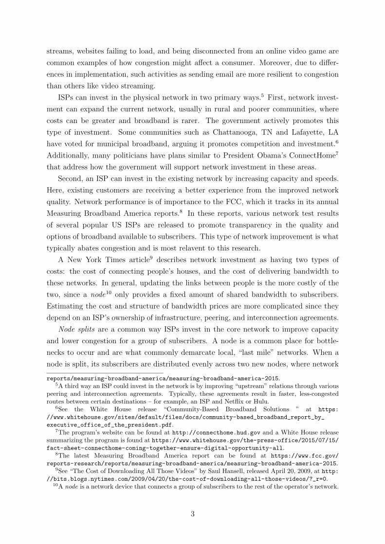
1 IntroductionThe Internet is now an ever-present part of society, and the demand for online content,

especially over-the-top (OTT) video, is soaring. Internet Service Providers (ISPs) choose

to invest and meet this demand when there is incentive to do so. An industry estimate

places private broadband investment around $1.3 trillion between 1996 and 2013, or about

$75 billion per year.1 Historically broadband investment has been financed by private

firms, but its importance is now leading some local governments to pursue municipal

broadband and other public funding to support further investment and competition.

In this paper, we provide a key input to understanding how responsive consumers

are to network congestion by estimating demand using a novel data set and variation in

network congestion and prices. Congested areas of the network are prime candidates for

investment because a consistently poor network could lead to welfare losses for consumers,

ISPs, and third-parties. In particular, we focus on congestion abatement and its value

to consumers. We believe these results are of particular importance to any public policy

debate that evaluates the value created by broadband investment. For example, as a part

of the Charter/Time Warner Cable merger review, broadband investment to modernize

and expand the network is a likely condition for approval.2

The unique data at the center of this work are made available by a North American

ISP. These data include hourly observations of Internet usage and network conditions

for roughly 45,000 subscribers from February 2015 through December 2015. At the daily

level, we are able to uniquely map an account to a cable modem and active Internet

plan. For each Internet plan, we observe the price, advertised speeds3 (downstream and

upstream), usage allowance, and overage fees. All data tiers charge for data overages at

the same per GB rate. The average subscriber in our data uses 2.3 gigabytes (GB) per

day, pays $58.89 for a 22 megabit per second (Mbps) downstream connection, and a 267

GB monthly usage allowance.

Network congestion occurs when demand pushes or exceeds the network’s limitations

– similar to how video streaming performance degrades if too many people utilize the

same WiFi connection. Aside from downstream and upstream speeds, the Federal Com-

munications Commission (FCC) recognizes latency (how long it takes requests to move

across the Internet) and packet loss (roughly, the percentage of requests that fail to make

it to their destination) as two important metrics of network performance.4 Buffering video

1See USTelecom’s estimates at http://www.ustelecom.org/broadband-industry-stats/

investment/historical-broadband-provider-capex and page 15 of the FCC’s 2015Broadband Progress Report found at https://www.fcc.gov/reports-research/reports/

broadband-progress-reports/2015-broadband-progress-report.2See the State of New York Public Service Commission’s Case 15-M–0388 on “Joint Petition of Charter

Communications and Time Warner Cable for Approval”, released on January 8, 2016.3Speed is measured in Megabits per second (Mbps). For reference, a 20 Mbps downstream connection

would download a 4 gigabyte file, or roughly one high-definition movie, in about 27 minutes.4See the FCC’s 2015 Measuring Broadband Report at https://www.fcc.gov/reports-research/

2

streams, websites failing to load, and being disconnected from an online video game are

common examples of how congestion might affect a consumer. Moreover, due to differ-

ences in implementation, such activities as sending email are more resilient to congestion

than others like video streaming.

ISPs can invest in the physical network in two primary ways.5 First, network invest-

ment can expand the current network, usually in rural and poorer communities, where

costs can be greater and broadband is rarer. The government actively promotes this

type of investment. Some communities such as Chattanooga, TN and Lafayette, LA

have voted for municipal broadband, arguing it promotes competition and investment.6

Additionally, many politicians have plans similar to President Obama’s ConnectHome7

that address how the government will support network investment in these areas.

Second, an ISP can invest in the existing network by increasing capacity and speeds.

Here, existing customers are receiving a better experience from the improved network

quality. Network performance is of importance to the FCC, which it tracks in its annual

Measuring Broadband America reports.8 In these reports, various network test results

of several popular US ISPs are released to promote transparency in the quality and

options of broadband available to subscribers. This type of network improvement is what

typically abates congestion and is most relavent to this research.

A New York Times article9 describes network investment as having two types of

costs: the cost of connecting people’s houses, and the cost of delivering bandwidth to

these networks. In general, updating the links between people is the more costly of the

two, since a node10 only provides a fixed amount of shared bandwidth to subscribers.

Estimating the cost and structure of bandwidth prices are more complicated since they

depend on an ISP’s ownership of infrastructure, peering, and interconnection agreements.

Node splits are a common way ISPs invest in the core network to improve capacity

and lower congestion for a group of subscribers. A node is a common place for bottle-

necks to occur and are what commonly demarcate local, “last mile” networks. When a

node is split, its subscribers are distributed evenly across two new nodes, where network

reports/measuring-broadband-america/measuring-broadband-america-2015.5A third way an ISP could invest in the network is by improving “upstream” relations through various

peering and interconnection agreements. Typically, these agreements result in faster, less-congestedroutes between certain destinations – for example, an ISP and Netflix or Hulu.

6See the White House release “Community-Based Broadband Solutions ” at https:

//www.whitehouse.gov/sites/default/files/docs/community-based_broadband_report_by_

executive_office_of_the_president.pdf.7The program’s website can be found at http://connecthome.hud.gov and a White House release

summarizing the program is found at https://www.whitehouse.gov/the-press-office/2015/07/15/fact-sheet-connecthome-coming-together-ensure-digital-opportunity-all.

8The latest Measuring Broadband America report can be found at https://www.fcc.gov/

reports-research/reports/measuring-broadband-america/measuring-broadband-america-2015.9See “The Cost of Downloading All Those Videos” by Saul Hansell, released April 20, 2009, at http:

//bits.blogs.nytimes.com/2009/04/20/the-cost-of-downloading-all-those-videos/?_r=0.10A node is a network device that connects a group of subscribers to the rest of the operator’s network.

3

conditions should be improved. Many operators target nodes to be split once average

utilization exceeds certain thresholds. We observe 5 node splits in our data and use these

events to compare before-and-after congestion and subscriber usage. After a split, av-

erage daily usage increases by 7% and packet loss, our measure of congestion, drops by

27%. This suggests there is value to consumers from a less congested network.

The value to consumers of less congestion only captures part of the rent created by the

investment: some goes back to the ISP and the rest goes to third-parties. In fact, since the

ISP is unable to fully capture these rents, private investment is marginally discouraged.

Moreover, recent Title II and net neutrality regulation by the FCC has created uncertainty

on the future of the industry, which could depress future investment. Tom Wheeler, the

current FCC chairman, declares Title II will have no effect on investment, while other

commissioners are doubtful.11

Our model of subscriber Internet consumption builds on the framework of Nevo et al.

(2016) with the notable difference being the inclusion of network congestion and its

impact on plan choice and consumption. Similarly, our estimation relies on variation in

prices and speeds across plans and (shadow) price variation across the billing cycle that

is created by usage-based pricing. We also utilize variation in a subscriber’s observed

packet loss to estimate the effect of congestion.

The price variation arising from usage-based pricing is a result of its three-part tariff

structure: a subscriber pays a fixed fee each month, and if the associated usage allowance

is exceeded, she is charged at a per GB rate thereafter. While overage fees are only

assessed if a subscriber exceeds the usage allowance, a forward-looking subscriber under-

stands today’s consumption marginally increases the likelihood of exceeding the usage

allowance before the end of the billing cycle – this is a function of how many days remain

in the billing cycle and what fraction of the usage allowance has been used previously in

the cycle. We incorporate these dynamics in our model similar to Nevo et al. (2016) by

allowing consumers to make daily consumption decisions across a billing cycle.

We also use variation in network congestion to identify a subscriber’s sensitivity to

poor network states. Our hourly data contain packet loss, or the percentage of total

packets requested that are either dropped or delayed, at the subscriber level, which we

use to proxy for network congestion. As mentioned previously, packet loss is one statistic

the FCC uses to benchmark network performance across ISPs.

There are four main advantages to using packet loss over other variables such as a

node’s utilization to measure congestion in our model. First, we observe packet loss at

a subscriber level, so it is not an aggregate network statistic. Second, we observe wide

cross-sectional variation in packet loss across subscribers. Third, packet loss is positively

11See Chairman Wheeler’s article “This is How We Will Ensure Net Neutrality” at http:

//www.wired.com/2015/02/fcc-chairman-wheeler-net-neutrality/, for example, and Commis-sionar Pai’s remarks on “Declining Broadband Investment” at https://www.fcc.gov/document/

comm-pai-remarks-declining-broadband-investment.

4

correlated with other common congestion variables. Fourth, our ISP invested in its

existing network throughout the year, so we are able to exploit time series variation in

our panel as well. Our ISP’s network would rate as the third worst in average subscriber

packet loss in the latest Measuring Broadband America. Coupled with the aforementioned

core network investments by the operator over 2015, this sample offers a wide range of

variation in network conditions, ideal for this analysis.

We estimate this finite horizon, dynamic choice model by solving the dynamic problem

once for a large number of types. The solution to these dynamic problems is then used

to estimate the distribution of types over our sample by minimizing the error between

observed and optimal behavior across types. In general, the estimated marginal and joint

distributions illustrate the strength of the flexibility built into our estimation approach.

Compared to Nevo et al. (2016)’s concentrated type distribution, ours is much more

uniform.

These demand estimates are used to measure the value to subscribers when network

congestion is eliminated entirely. This is the case where a subscriber’s provisioned speed

is always realized. We find the improved network conditions encourage some subscribers

to downgrade to cheaper plans, but the loss in revenue from this is entirely offset by

an increase in consumer surplus. Subscribers’ realized speeds increased by roughly 19%

with each additional Mbps of speed being valued at roughly $2.87. These results suggest

that when public policy focuses on network investment, congestion abatement should be

considered because of this positive value enjoyed by subscribers.

This paper is most closely related to a literature that studies the demand of residential

broadband. Recent examples are Nevo et al. (2016), Malone et al. (2016), and Malone

et al. (2014) that use similar high-frequency data to study subscriber behavior. However,

this literature dates back to the early 2000s with Varian (2002) and Edell and Varaiya

(2002), who run experiments where consumers face different prices for varying allowances

and speeds. Goolsbee and Klenow (2006) estimate the benefit to residential broadband;

Hitte and Tambe (2007) show Internet usage increases by roughly 22 hours per month

when broadband is introduced. Other related papers are Lambrecht et al. (2007), Dutz

et al. (2009), Rosston et al. (2013), and Greenstein and McDevitt (2011).

2 DataThe data for our analysis come from a representative sample of 46,667 North American

broadband subscribers. The metropolitan area where the subscribers are drawn from

have demographic characteristics that are similar to the entire US population, its average

income is within 10% of the national average and the demographic composition is similar

to the overall US population. Therefore, we expect the insights from our analysis to have

external validity in other North American markets. The data include hourly subscriber

usage and details of network conditions for February–December 2015.

5

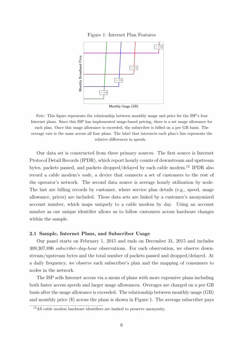
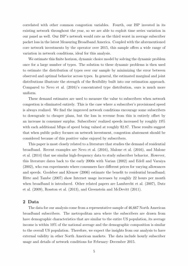
Figure 1: Internet Plan Features

Monthly Usage (GB)

MonthlyBroadband

Price

∼ 1.0

∼ 2.0

∼ 3.5

∼ 7.0

Note: This figure represents the relationship between monthly usage and price for the ISP’s four

Internet plans. Since this ISP has implemented usage-based pricing, there is a set usage allowance for

each plan. Once this usage allowance is exceeded, the subscriber is billed on a per GB basis. The

overage rate is the same across all four plans. The label that intersects each plan’s line represents the

relative differences in speeds.

Our data set is constructed from three primary sources. The first source is Internet

Protocol Detail Records (IPDR), which report hourly counts of downstream and upstream

bytes, packets passed, and packets dropped/delayed by each cable modem.12 IPDR also

record a cable modem’s node, a device that connects a set of customers to the rest of

the operator’s network. The second data source is average hourly utilization by node.

The last are billing records by customer, where service plan details (e.g., speed, usage

allowance, prices) are included. These data sets are linked by a customer’s anonymized

account number, which maps uniquely to a cable modem by day. Using an account

number as our unique identifier allows us to follow customers across hardware changes

within the sample.

2.1 Sample, Internet Plans, and Subscriber Usage

Our panel starts on February 1, 2015 and ends on December 31, 2015 and includes

309,307,896 subscriber -day-hour observations. For each observation, we observe down-

stream/upstream bytes and the total number of packets passed and dropped/delayed. At

a daily frequency, we observe each subscriber’s plan and the mapping of consumers to

nodes in the network.

The ISP sells Internet access via a menu of plans with more expensive plans including

both faster access speeds and larger usage allowances. Overages are charged on a per GB

basis after the usage allowance is exceeded. The relationship between monthly usage (GB)

and monthly price ($) across the plans is shown in Figure 1. The average subscriber pays

12All cable modem hardware identifiers are hashed to preserve anonymity.

6

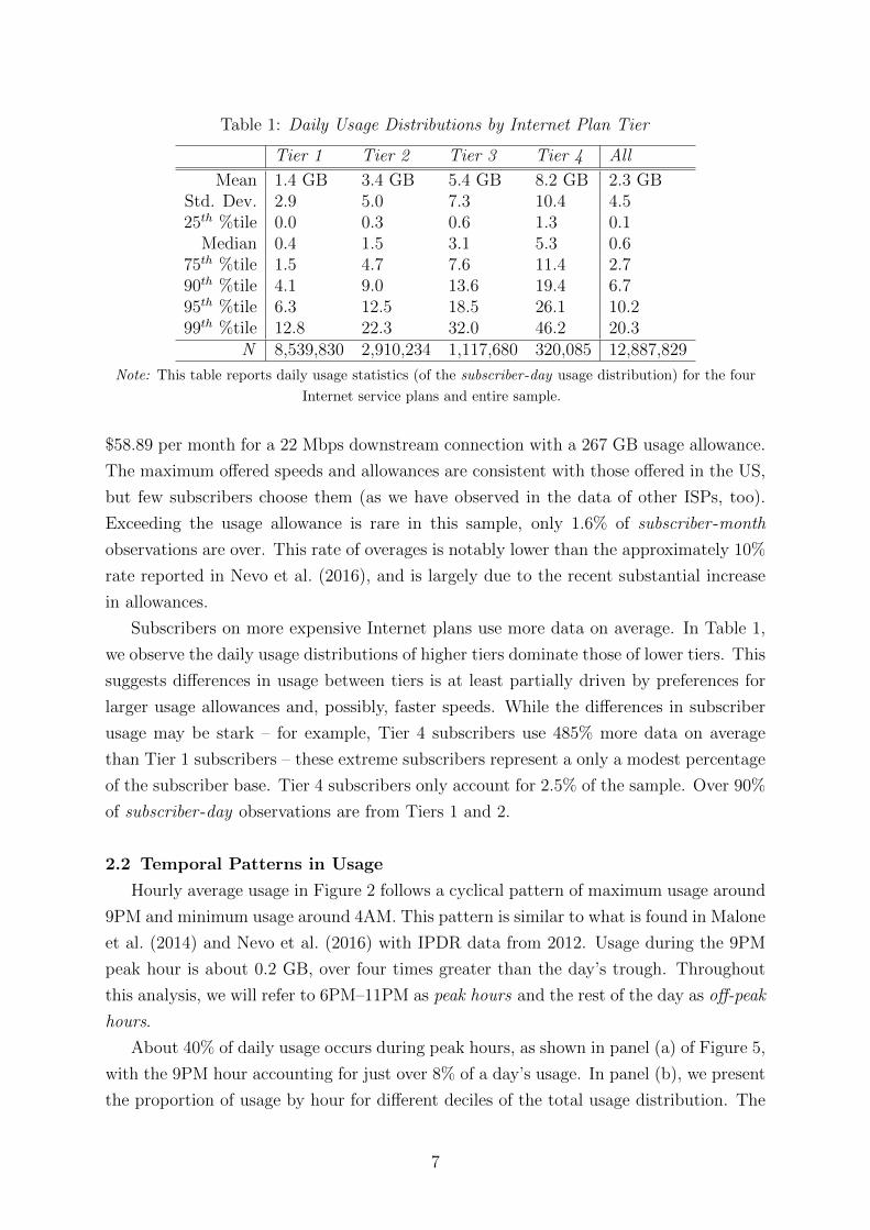
Table 1: Daily Usage Distributions by Internet Plan Tier

Tier 1 Tier 2 Tier 3 Tier 4 All

Mean 1.4 GB 3.4 GB 5.4 GB 8.2 GB 2.3 GBStd. Dev. 2.9 5.0 7.3 10.4 4.525th %tile 0.0 0.3 0.6 1.3 0.1

Median 0.4 1.5 3.1 5.3 0.675th %tile 1.5 4.7 7.6 11.4 2.790th %tile 4.1 9.0 13.6 19.4 6.795th %tile 6.3 12.5 18.5 26.1 10.299th %tile 12.8 22.3 32.0 46.2 20.3

N 8,539,830 2,910,234 1,117,680 320,085 12,887,829

Note: This table reports daily usage statistics (of the subscriber -day usage distribution) for the four

Internet service plans and entire sample.

$58.89 per month for a 22 Mbps downstream connection with a 267 GB usage allowance.

The maximum offered speeds and allowances are consistent with those offered in the US,

but few subscribers choose them (as we have observed in the data of other ISPs, too).

Exceeding the usage allowance is rare in this sample, only 1.6% of subscriber -month

observations are over. This rate of overages is notably lower than the approximately 10%

rate reported in Nevo et al. (2016), and is largely due to the recent substantial increase

in allowances.

Subscribers on more expensive Internet plans use more data on average. In Table 1,

we observe the daily usage distributions of higher tiers dominate those of lower tiers. This

suggests differences in usage between tiers is at least partially driven by preferences for

larger usage allowances and, possibly, faster speeds. While the differences in subscriber

usage may be stark – for example, Tier 4 subscribers use 485% more data on average

than Tier 1 subscribers – these extreme subscribers represent a only a modest percentage

of the subscriber base. Tier 4 subscribers only account for 2.5% of the sample. Over 90%

of subscriber -day observations are from Tiers 1 and 2.

2.2 Temporal Patterns in Usage

Hourly average usage in Figure 2 follows a cyclical pattern of maximum usage around

9PM and minimum usage around 4AM. This pattern is similar to what is found in Malone

et al. (2014) and Nevo et al. (2016) with IPDR data from 2012. Usage during the 9PM

peak hour is about 0.2 GB, over four times greater than the day’s trough. Throughout

this analysis, we will refer to 6PM–11PM as peak hours and the rest of the day as off-peak

hours.

About 40% of daily usage occurs during peak hours, as shown in panel (a) of Figure 5,

with the 9PM hour accounting for just over 8% of a day’s usage. In panel (b), we present

the proportion of usage by hour for different deciles of the total usage distribution. The

7

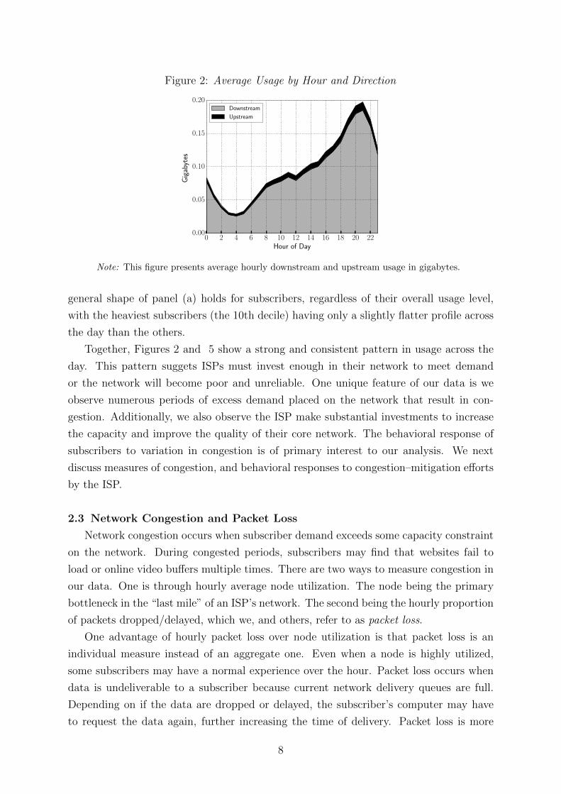
Figure 2: Average Usage by Hour and Direction

0 2 4 6 8 10 12 14 16 18 20 22Hour of Day

0.00

0.05

0.10

0.15

0.20

Gigabytes

Downstream

Upstream

Note: This figure presents average hourly downstream and upstream usage in gigabytes.

general shape of panel (a) holds for subscribers, regardless of their overall usage level,

with the heaviest subscribers (the 10th decile) having only a slightly flatter profile across

the day than the others.

Together, Figures 2 and 5 show a strong and consistent pattern in usage across the

day. This pattern suggets ISPs must invest enough in their network to meet demand

or the network will become poor and unreliable. One unique feature of our data is we

observe numerous periods of excess demand placed on the network that result in con-

gestion. Additionally, we also observe the ISP make substantial investments to increase

the capacity and improve the quality of their core network. The behavioral response of

subscribers to variation in congestion is of primary interest to our analysis. We next

discuss measures of congestion, and behavioral responses to congestion–mitigation efforts

by the ISP.

2.3 Network Congestion and Packet Loss

Network congestion occurs when subscriber demand exceeds some capacity constraint

on the network. During congested periods, subscribers may find that websites fail to

load or online video buffers multiple times. There are two ways to measure congestion in

our data. One is through hourly average node utilization. The node being the primary

bottleneck in the “last mile” of an ISP’s network. The second being the hourly proportion

of packets dropped/delayed, which we, and others, refer to as packet loss.

One advantage of hourly packet loss over node utilization is that packet loss is an

individual measure instead of an aggregate one. Even when a node is highly utilized,

some subscribers may have a normal experience over the hour. Packet loss occurs when

data is undeliverable to a subscriber because current network delivery queues are full.

Depending on if the data are dropped or delayed, the subscriber’s computer may have

to request the data again, further increasing the time of delivery. Packet loss is more

8

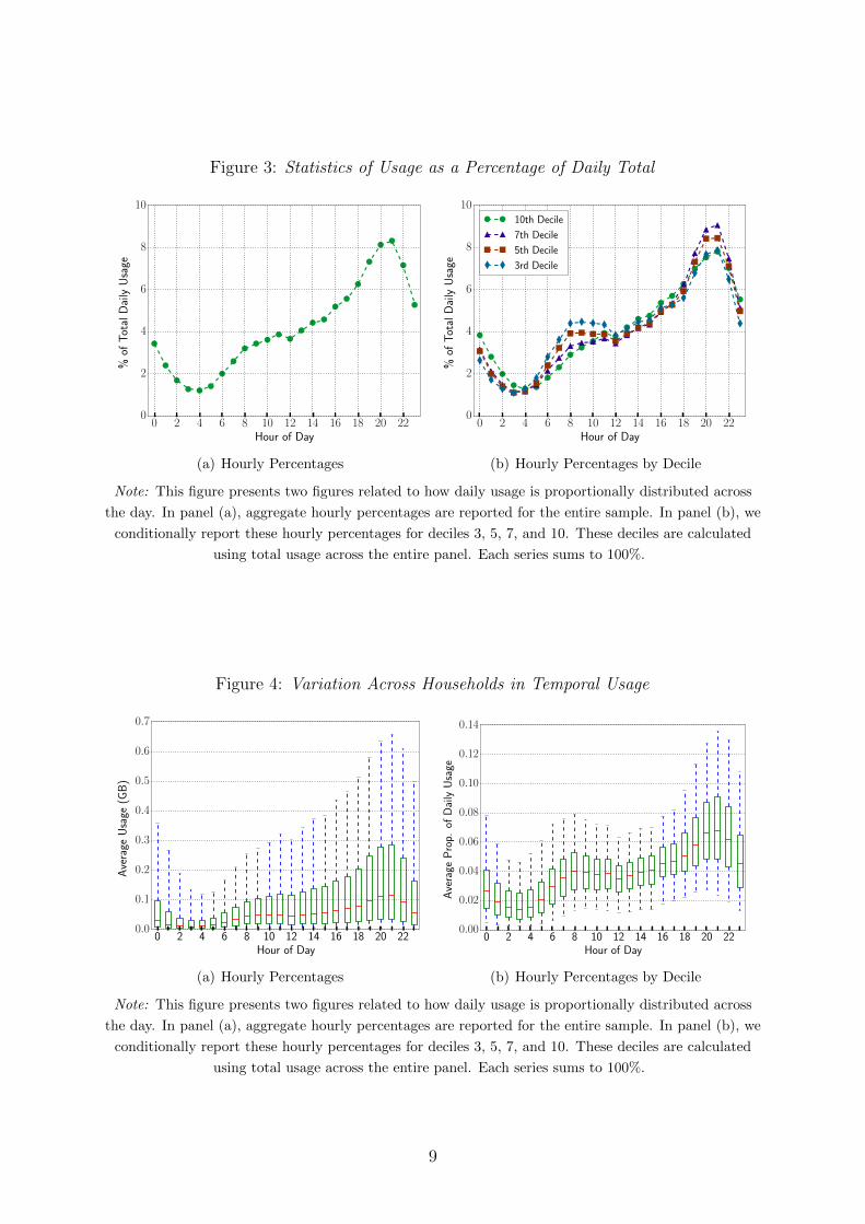
Figure 3: Statistics of Usage as a Percentage of Daily Total

0 2 4 6 8 10 12 14 16 18 20 22Hour of Day

0

2

4

6

8

10

%of

TotalDailyUsage

(a) Hourly Percentages

0 2 4 6 8 10 12 14 16 18 20 22Hour of Day

0

2

4

6

8

10

%of

TotalDailyUsage

10th Decile

7th Decile

5th Decile

3rd Decile

(b) Hourly Percentages by Decile

Note: This figure presents two figures related to how daily usage is proportionally distributed across

the day. In panel (a), aggregate hourly percentages are reported for the entire sample. In panel (b), we

conditionally report these hourly percentages for deciles 3, 5, 7, and 10. These deciles are calculated

using total usage across the entire panel. Each series sums to 100%.

Figure 4: Variation Across Households in Temporal Usage

0 2 4 6 8 10 12 14 16 18 20 22Hour of Day

0.0

0.1

0.2

0.3

0.4

0.5

0.6

0.7

Average

Usage

(GB)

(a) Hourly Percentages

0 2 4 6 8 10 12 14 16 18 20 22Hour of Day

0.00

0.02

0.04

0.06

0.08

0.10

0.12

0.14

Average

Prop.

ofDailyUsage

(b) Hourly Percentages by Decile

Note: This figure presents two figures related to how daily usage is proportionally distributed across

the day. In panel (a), aggregate hourly percentages are reported for the entire sample. In panel (b), we

conditionally report these hourly percentages for deciles 3, 5, 7, and 10. These deciles are calculated

using total usage across the entire panel. Each series sums to 100%.

9

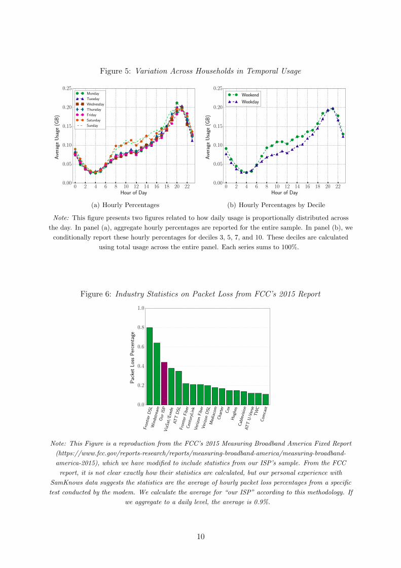
Figure 5: Variation Across Households in Temporal Usage

0 2 4 6 8 10 12 14 16 18 20 22Hour of Day

0.00

0.05

0.10

0.15

0.20

0.25

Average

Usage

(GB)

Monday

Tuesday

Wednesday

Thursday

Friday

Saturday

Sunday

(a) Hourly Percentages

0 2 4 6 8 10 12 14 16 18 20 22Hour of Day

0.00

0.05

0.10

0.15

0.20

0.25

Average

Usage

(GB)

Weekend

Weekday

(b) Hourly Percentages by Decile

Note: This figure presents two figures related to how daily usage is proportionally distributed across

the day. In panel (a), aggregate hourly percentages are reported for the entire sample. In panel (b), we

conditionally report these hourly percentages for deciles 3, 5, 7, and 10. These deciles are calculated

using total usage across the entire panel. Each series sums to 100%.

Figure 6: Industry Statistics on Packet Loss from FCC’s 2015 Report

FrontierDSL

Windstream

Our

ISP

ViaSat/E

xede

ATTDSL

Fronter

Fiber

CenturyLink

Verizon

Fiber

Verizon

DSL

Mediacom

Charter

Cox

Hughes

Cablevision

ATTU-Verse

TWC

Com

cast

0.0

0.2

0.4

0.6

0.8

1.0

PacketLossPercentage

Note: This Figure is a reproduction from the FCC’s 2015 Measuring Broadband America Fixed Report

(https://www.fcc.gov/reports-research/reports/measuring-broadband-america/measuring-broadband-

america-2015), which we have modified to include statistics from our ISP’s sample. From the FCC

report, it is not clear exactly how their statistics are calculated, but our personal experience with

SamKnows data suggests the statistics are the average of hourly packet loss percentages from a specific

test conducted by the modem. We calculate the average for “our ISP” according to this methodology. If

we aggregate to a daily level, the average is 0.9%.

10

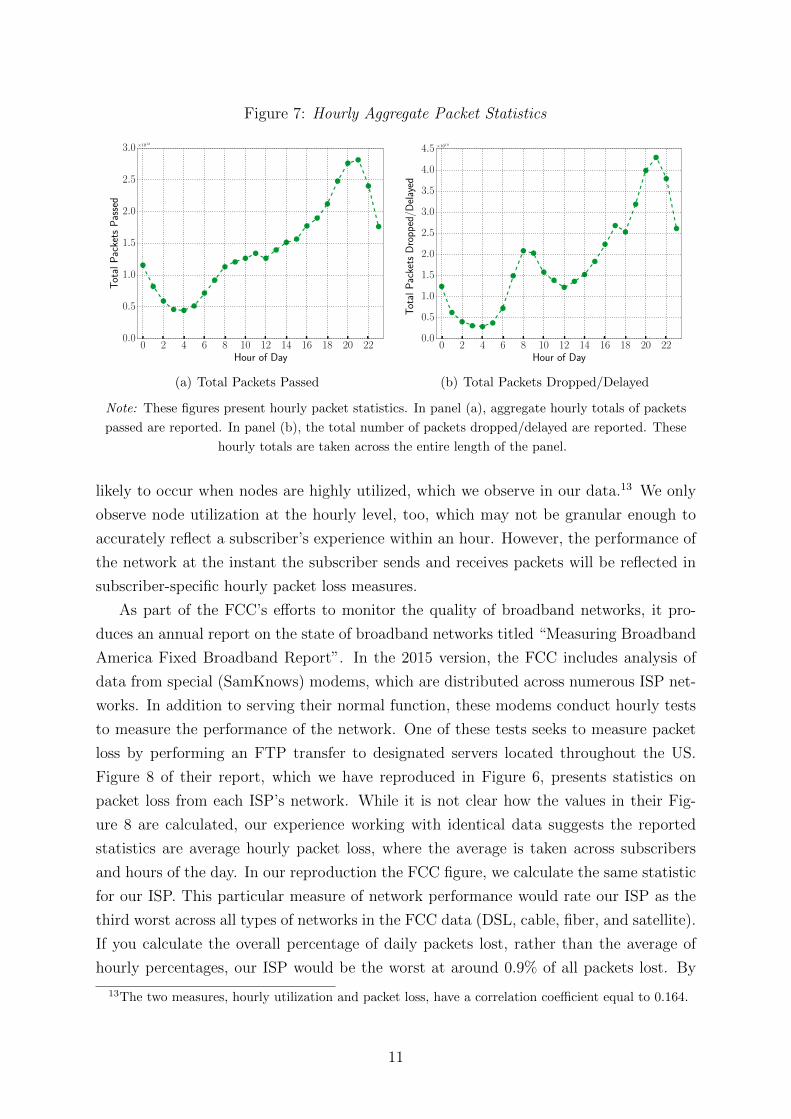
Figure 7: Hourly Aggregate Packet Statistics

0 2 4 6 8 10 12 14 16 18 20 22Hour of Day

0.0

0.5

1.0

1.5

2.0

2.5

3.0

TotalPackets

Passed

×1012

(a) Total Packets Passed

0 2 4 6 8 10 12 14 16 18 20 22Hour of Day

0.0

0.5

1.0

1.5

2.0

2.5

3.0

3.5

4.0

4.5

TotalPackets

Dropped/D

elayed

×1010

(b) Total Packets Dropped/Delayed

Note: These figures present hourly packet statistics. In panel (a), aggregate hourly totals of packets

passed are reported. In panel (b), the total number of packets dropped/delayed are reported. These

hourly totals are taken across the entire length of the panel.

likely to occur when nodes are highly utilized, which we observe in our data.13 We only

observe node utilization at the hourly level, too, which may not be granular enough to

accurately reflect a subscriber’s experience within an hour. However, the performance of

the network at the instant the subscriber sends and receives packets will be reflected in

subscriber-specific hourly packet loss measures.

As part of the FCC’s efforts to monitor the quality of broadband networks, it pro-

duces an annual report on the state of broadband networks titled “Measuring Broadband

America Fixed Broadband Report”. In the 2015 version, the FCC includes analysis of

data from special (SamKnows) modems, which are distributed across numerous ISP net-

works. In addition to serving their normal function, these modems conduct hourly tests

to measure the performance of the network. One of these tests seeks to measure packet

loss by performing an FTP transfer to designated servers located throughout the US.

Figure 8 of their report, which we have reproduced in Figure 6, presents statistics on

packet loss from each ISP’s network. While it is not clear how the values in their Fig-

ure 8 are calculated, our experience working with identical data suggests the reported

statistics are average hourly packet loss, where the average is taken across subscribers

and hours of the day. In our reproduction the FCC figure, we calculate the same statistic

for our ISP. This particular measure of network performance would rate our ISP as the

third worst across all types of networks in the FCC data (DSL, cable, fiber, and satellite).

If you calculate the overall percentage of daily packets lost, rather than the average of

hourly percentages, our ISP would be the worst at around 0.9% of all packets lost. By

13The two measures, hourly utilization and packet loss, have a correlation coefficient equal to 0.164.

11

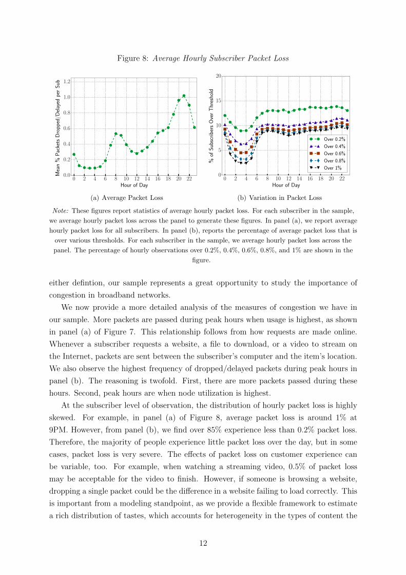
Figure 8: Average Hourly Subscriber Packet Loss

0 2 4 6 8 10 12 14 16 18 20 22Hour of Day

0.0

0.2

0.4

0.6

0.8

1.0

1.2

Mean%

Packets

Dropped/D

elayed

per

Sub

(a) Average Packet Loss

0 2 4 6 8 10 12 14 16 18 20 22Hour of Day

0

5

10

15

20

%of

SubscribersOverThreshold

Over 0.2%

Over 0.4%

Over 0.6%

Over 0.8%

Over 1%

(b) Variation in Packet Loss

Note: These figures report statistics of average hourly packet loss. For each subscriber in the sample,

we average hourly packet loss across the panel to generate these figures. In panel (a), we report average

hourly packet loss for all subscribers. In panel (b), reports the percentage of average packet loss that is

over various thresholds. For each subscriber in the sample, we average hourly packet loss across the

panel. The percentage of hourly observations over 0.2%, 0.4%, 0.6%, 0.8%, and 1% are shown in the

figure.

either defintion, our sample represents a great opportunity to study the importance of

congestion in broadband networks.

We now provide a more detailed analysis of the measures of congestion we have in

our sample. More packets are passed during peak hours when usage is highest, as shown

in panel (a) of Figure 7. This relationship follows from how requests are made online.

Whenever a subscriber requests a website, a file to download, or a video to stream on

the Internet, packets are sent between the subscriber’s computer and the item’s location.

We also observe the highest frequency of dropped/delayed packets during peak hours in

panel (b). The reasoning is twofold. First, there are more packets passed during these

hours. Second, peak hours are when node utilization is highest.

At the subscriber level of observation, the distribution of hourly packet loss is highly

skewed. For example, in panel (a) of Figure 8, average packet loss is around 1% at

9PM. However, from panel (b), we find over 85% experience less than 0.2% packet loss.

Therefore, the majority of people experience little packet loss over the day, but in some

cases, packet loss is very severe. The effects of packet loss on customer experience can

be variable, too. For example, when watching a streaming video, 0.5% of packet loss

may be acceptable for the video to finish. However, if someone is browsing a website,

dropping a single packet could be the difference in a website failing to load correctly. This

is important from a modeling standpoint, as we provide a flexible framework to estimate

a rich distribution of tastes, which accounts for heterogeneity in the types of content the

12

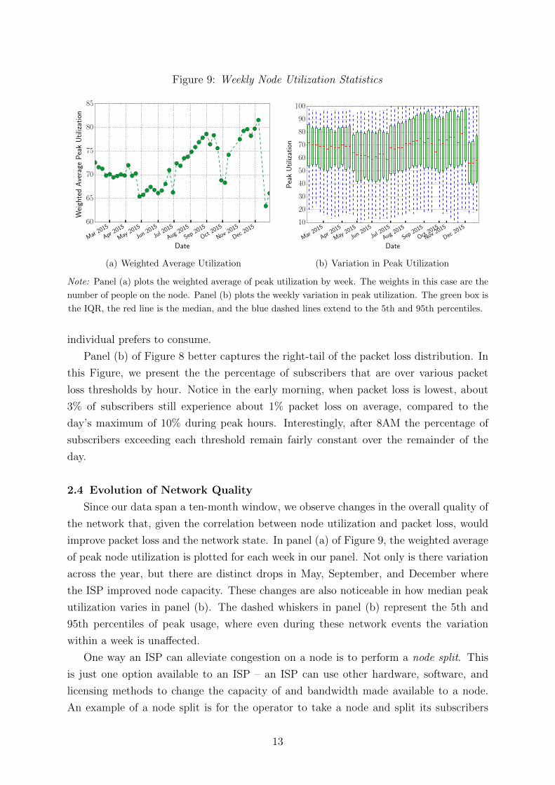
Figure 9: Weekly Node Utilization Statistics

Mar 2015

Apr 2015

May 2

015

Jun201

5

Jul201

5

Aug 2

015

Sep201

5

Oct 2

015

Nov 2

015

Dec 2

015

Date

60

65

70

75

80

85

WeightedAverage

PeakUtilization

(a) Weighted Average Utilization

Mar 2015

Apr 2015

May 2

015

Jun201

5

Jul201

5

Aug 2

015

Sep201

5

Oct 2

015

Nov 2

015

Dec 2

015

Date

10

20

30

40

50

60

70

80

90

100

PeakUtilization

(b) Variation in Peak Utilization

Note: Panel (a) plots the weighted average of peak utilization by week. The weights in this case are the

number of people on the node. Panel (b) plots the weekly variation in peak utilization. The green box is

the IQR, the red line is the median, and the blue dashed lines extend to the 5th and 95th percentiles.

individual prefers to consume.

Panel (b) of Figure 8 better captures the right-tail of the packet loss distribution. In

this Figure, we present the the percentage of subscribers that are over various packet

loss thresholds by hour. Notice in the early morning, when packet loss is lowest, about

3% of subscribers still experience about 1% packet loss on average, compared to the

day’s maximum of 10% during peak hours. Interestingly, after 8AM the percentage of

subscribers exceeding each threshold remain fairly constant over the remainder of the

day.

2.4 Evolution of Network Quality

Since our data span a ten-month window, we observe changes in the overall quality of

the network that, given the correlation between node utilization and packet loss, would

improve packet loss and the network state. In panel (a) of Figure 9, the weighted average

of peak node utilization is plotted for each week in our panel. Not only is there variation

across the year, but there are distinct drops in May, September, and December where

the ISP improved node capacity. These changes are also noticeable in how median peak

utilization varies in panel (b). The dashed whiskers in panel (b) represent the 5th and

95th percentiles of peak usage, where even during these network events the variation

within a week is unaffected.

One way an ISP can alleviate congestion on a node is to perform a node split. This

is just one option available to an ISP – an ISP can use other hardware, software, and

licensing methods to change the capacity of and bandwidth made available to a node.

An example of a node split is for the operator to take a node and split its subscribers

13

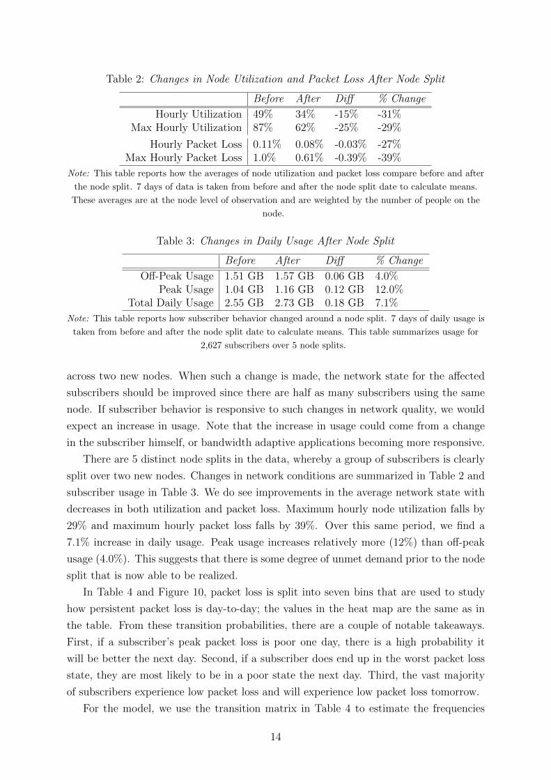
Table 2: Changes in Node Utilization and Packet Loss After Node Split

Before After Diff % Change

Hourly Utilization 49% 34% -15% -31%Max Hourly Utilization 87% 62% -25% -29%

Hourly Packet Loss 0.11% 0.08% -0.03% -27%Max Hourly Packet Loss 1.0% 0.61% -0.39% -39%

Note: This table reports how the averages of node utilization and packet loss compare before and after

the node split. 7 days of data is taken from before and after the node split date to calculate means.

These averages are at the node level of observation and are weighted by the number of people on the

node.

Table 3: Changes in Daily Usage After Node Split

Before After Diff % Change

Off-Peak Usage 1.51 GB 1.57 GB 0.06 GB 4.0%Peak Usage 1.04 GB 1.16 GB 0.12 GB 12.0%

Total Daily Usage 2.55 GB 2.73 GB 0.18 GB 7.1%

Note: This table reports how subscriber behavior changed around a node split. 7 days of daily usage is

taken from before and after the node split date to calculate means. This table summarizes usage for

2,627 subscribers over 5 node splits.

across two new nodes. When such a change is made, the network state for the affected

subscribers should be improved since there are half as many subscribers using the same

node. If subscriber behavior is responsive to such changes in network quality, we would

expect an increase in usage. Note that the increase in usage could come from a change

in the subscriber himself, or bandwidth adaptive applications becoming more responsive.

There are 5 distinct node splits in the data, whereby a group of subscribers is clearly

split over two new nodes. Changes in network conditions are summarized in Table 2 and

subscriber usage in Table 3. We do see improvements in the average network state with

decreases in both utilization and packet loss. Maximum hourly node utilization falls by

29% and maximum hourly packet loss falls by 39%. Over this same period, we find a

7.1% increase in daily usage. Peak usage increases relatively more (12%) than off-peak

usage (4.0%). This suggests that there is some degree of unmet demand prior to the node

split that is now able to be realized.

In Table 4 and Figure 10, packet loss is split into seven bins that are used to study

how persistent packet loss is day-to-day; the values in the heat map are the same as in

the table. From these transition probabilities, there are a couple of notable takeaways.

First, if a subscriber’s peak packet loss is poor one day, there is a high probability it

will be better the next day. Second, if a subscriber does end up in the worst packet loss

state, they are most likely to be in a poor state the next day. Third, the vast majority

of subscribers experience low packet loss and will experience low packet loss tomorrow.

For the model, we use the transition matrix in Table 4 to estimate the frequencies

14

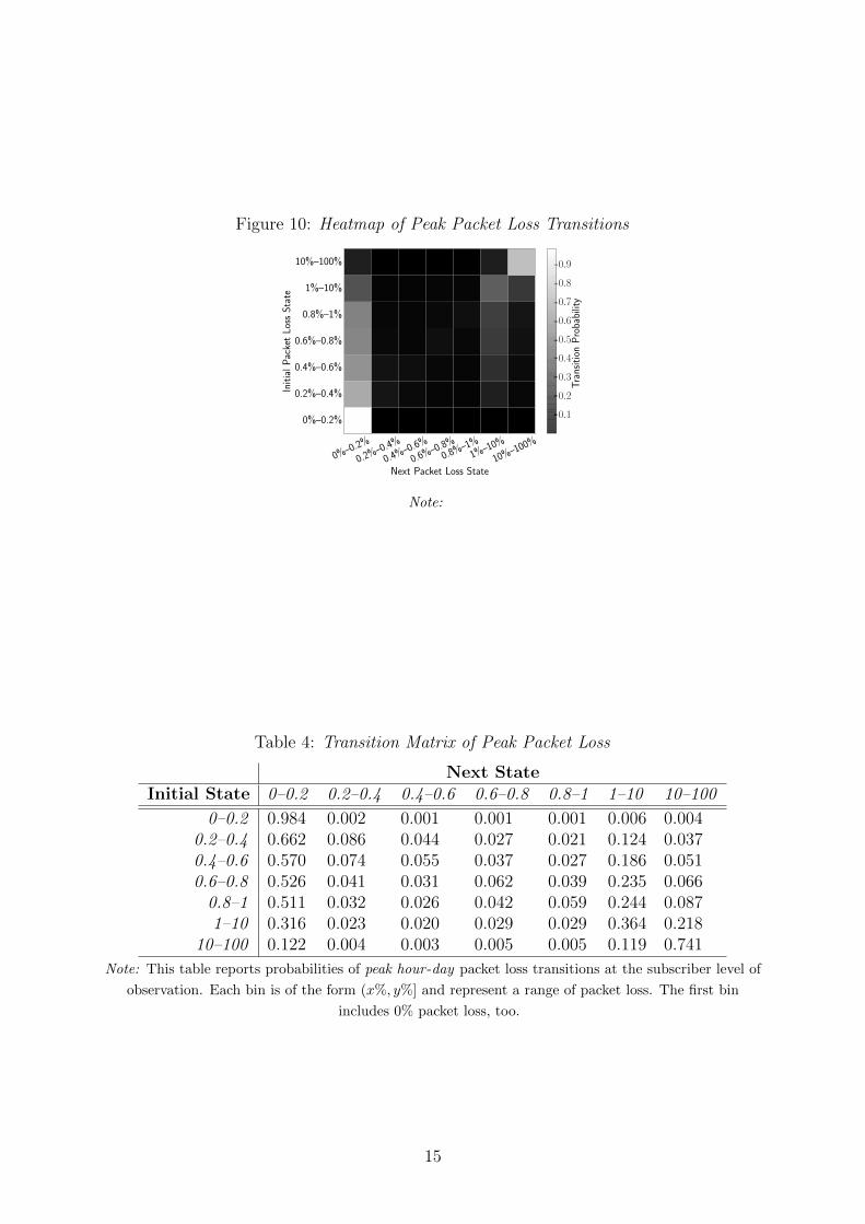
Figure 10: Heatmap of Peak Packet Loss Transitions

0%–0.

2%

0.2%–

0.4%

0.4%–

0.6%

0.6%–

0.8%0.8

%–1%1%

–10%

10%–10

0%

Next Packet Loss State

0%–0.2%

0.2%–0.4%

0.4%–0.6%

0.6%–0.8%

0.8%–1%

1%–10%

10%–100%

InitialPacketLossState

0.1

0.2

0.3

0.4

0.5

0.6

0.7

0.8

0.9

TransitionProbability

Note:

Table 4: Transition Matrix of Peak Packet Loss

Next StateInitial State 0–0.2 0.2–0.4 0.4–0.6 0.6–0.8 0.8–1 1–10 10–100

0–0.2 0.984 0.002 0.001 0.001 0.001 0.006 0.0040.2–0.4 0.662 0.086 0.044 0.027 0.021 0.124 0.0370.4–0.6 0.570 0.074 0.055 0.037 0.027 0.186 0.0510.6–0.8 0.526 0.041 0.031 0.062 0.039 0.235 0.066

0.8–1 0.511 0.032 0.026 0.042 0.059 0.244 0.0871–10 0.316 0.023 0.020 0.029 0.029 0.364 0.218

10–100 0.122 0.004 0.003 0.005 0.005 0.119 0.741

Note: This table reports probabilities of peak hour -day packet loss transitions at the subscriber level of

observation. Each bin is of the form (x%, y%] and represent a range of packet loss. The first bin

includes 0% packet loss, too.

15

of transition between packet loss, or network congestion, states. Below in the model

discussion, this will beGψ. This matrix will be used to solve the model. For the estimation

procedure, all we need are day-hour observations of daily consumption and the observed

peak packet loss state for each account in the sample.

3 ModelOur model builds on the model of Nevo et al. (2016). Like Nevo et al. (2016), we

assume a finite horizon, that a subscriber’s discount rate is β, and that a subscriber

makes a consumption decision each period on his optimally chosen plan. The primary

difference between the two models is we include network congestion and allow for it to

impact subscribers’ plan and consumption choices.

Given that our focus is on the role of congestion, we limit our sample to only sub-

scribers who never switched plans over the duration of the panel. This does not affect our

analysis for two reasons. First, service plans were upgraded shortly before our sample,

and, second, about 90% of subscribers made no changes during our period of observa-

tion. Allowing for plan switching introduces a dependency across billing cycles in the

dynamic problem, and by not modeling it the computational burden of solving the model

is reduced.14

3.1 Subscriber Utility From Content

Subscribers derive utility from consumption of content. Each day of a billing cycle,

t = 1....T , a subscriber chooses the amount of content to consume on their chosen service

plan, k = 1, ..., K. Plans are characterized by a provisioned speed content is delivered, sk,

by a usage allowance, Ck, by a fixed fee Fk that pays for all usage up to the allowance and

by an overage price, pk, per GB of usage in excess of the allowance. The menu of plans,

and the characteristics of each, are fixed.15 The provisioned speed is impacted by the

state of the network, ψ, which changes daily due to variation in congestion and frequent

network upgrades. We assume this evolution follows a first-order Markov process, Gψ.

Estimates of this process are presented in Table 4.

Utility from content is additively separable over all days in the billing cycle, and

across billing cycles.16 Let daily consumption of content be denoted by c. The utility for

14We explore the impact of relaxing this assumption in the Appendix by permitting customers toswitch plans once at the beginning of each billing cycle, and including the excluded customers in oursample. We find little impact on our results.

15Plans were changed months prior to our sample, but unchanged during our sample, and the ISP hadno plans to change them in the months after our sample ends.

16In this way, we assume content with a similar marginal utility is generated each day or constantlyrefreshed. This may not be the case for a subscriber who has not previously had access to the Internet.Below we will assume decreasing marginal utility within a time period, but additive across periods.

16

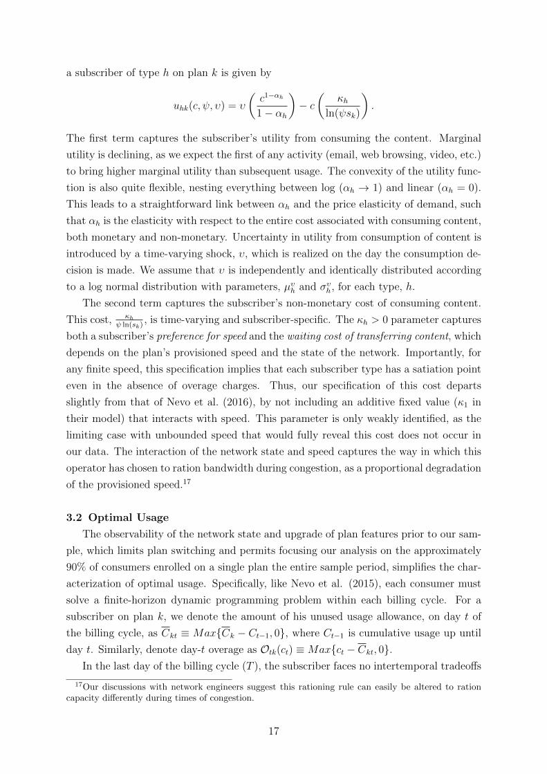
a subscriber of type h on plan k is given by

uhk(c, ψ, υ) = υ

(c1−αh

1− αh

)− c

(κh

ln(ψsk)

).

The first term captures the subscriber’s utility from consuming the content. Marginal

utility is declining, as we expect the first of any activity (email, web browsing, video, etc.)

to bring higher marginal utility than subsequent usage. The convexity of the utility func-

tion is also quite flexible, nesting everything between log (αh → 1) and linear (αh = 0).

This leads to a straightforward link between αh and the price elasticity of demand, such

that αh is the elasticity with respect to the entire cost associated with consuming content,

both monetary and non-monetary. Uncertainty in utility from consumption of content is

introduced by a time-varying shock, υ, which is realized on the day the consumption de-

cision is made. We assume that υ is independently and identically distributed according

to a log normal distribution with parameters, µυh and συh, for each type, h.

The second term captures the subscriber’s non-monetary cost of consuming content.

This cost, κhψ ln(sk)

, is time-varying and subscriber-specific. The κh > 0 parameter captures

both a subscriber’s preference for speed and the waiting cost of transferring content, which

depends on the plan’s provisioned speed and the state of the network. Importantly, for

any finite speed, this specification implies that each subscriber type has a satiation point

even in the absence of overage charges. Thus, our specification of this cost departs

slightly from that of Nevo et al. (2016), by not including an additive fixed value (κ1 in

their model) that interacts with speed. This parameter is only weakly identified, as the

limiting case with unbounded speed that would fully reveal this cost does not occur in

our data. The interaction of the network state and speed captures the way in which this

operator has chosen to ration bandwidth during congestion, as a proportional degradation

of the provisioned speed.17

3.2 Optimal Usage

The observability of the network state and upgrade of plan features prior to our sam-

ple, which limits plan switching and permits focusing our analysis on the approximately

90% of consumers enrolled on a single plan the entire sample period, simplifies the char-

acterization of optimal usage. Specifically, like Nevo et al. (2015), each consumer must

solve a finite-horizon dynamic programming problem within each billing cycle. For a

subscriber on plan k, we denote the amount of his unused usage allowance, on day t of

the billing cycle, as Ckt ≡ Max{Ck − Ct−1, 0}, where Ct−1 is cumulative usage up until

day t. Similarly, denote day-t overage as Otk(ct) ≡Max{ct − Ckt, 0}.In the last day of the billing cycle (T ), the subscriber faces no intertemporal tradeoffs

17Our discussions with network engineers suggest this rationing rule can easily be altered to rationcapacity differently during times of congestion.

17

and solves a static optimization problem, conditional on his cumulative usage CT−1 and

the realization of the preference shock, υT . Once υT is realized, subscribers who will

not incur overage charges (i.e., CkT is high) consume such that ∂uh(ct,yt,υt;k)∂ct

= 0. If∂uh(ct,yt,υt;k)

∂ctat ct = CkT is positive and less than pk, then consuming the remaining

allowance is optimal. For those subscribers above the allowance (i.e., CkT = 0) and a

high realization of υT , it is optimal to consume such that ∂uh(ct,yt,υt;k)∂ct

= pk. Denote

this optimal level of consumption in each scenario by c∗hkT (CT−1, υT ). Given this optimal

policy for consumption, utility in the terminal period is

VhkT (CT−1, ψT , υT ) =υT

((c∗hkT )1−αh

1− αh

)− c∗hkT

(κh

ln(ψtsk)

)− pkOtk(c∗hkT ).

For other days in the billing period, t < T , consumption increases cumulative con-

sumption and alters the state, so the optimal policy for a subscriber must incorporate

this. The optimal policy for any t < T can be expressed recursively such that for type h

on plan k

c∗hkt(Ct−1, ψt, υt) = argmaxct

{υt

(c1−αht

1−αh

)− ct

(κh

ln(ψtsk)

)− pkOtk(ct) + Eψ

[Vhk(t+1)(Ct−1 + ct, ψt+1)

]}.

Alternatively, defining the shadow price of consumption as

pk(ct, Ct−1, ψt) =

pk if Otk(ct) > 0

dEψ [Vhk(t+1)(Ct−1+ct,ψt+1)]

dctif Otk(ct) = 0 .

the optimal consumption choice in period t satisfies

c∗hkt =

(υt

κhln(ψtsk)

+ pk(c∗hkt, Ct−1, ψt)

) 1αh

. (1)

The relationship between αh and the price elasticity of usage is clear from Equation 1.

A type with parameter αh has a usage elasticity equal to − 1αh

with respect to the entire

marginal cost of content, κhln(ψtsk)

+ pk(ct, Ct−1, ψt).

The value function associated with the optimal usage policy is

Vhkt(Ct−1, ψt, υt) = υt

((c∗hkt)

1−αh

1−αh

)− c∗hkt

(κh

ln(ψtsk)

)− pkOt (c∗hkt) + Eψ

[Vhk(t+1)(Ct−1 + c∗hkt, ψt+1)

]

18

for each 3-tuple, (Ct−1, ψt, υt). Then for all t < T , the expected continuation value is

Eψ [Vhkt(Ct−1, ψt+1)] =

∫ψ

∫υ

Vhkt(Ct−1, ψt+1, υt)dGhυ(υt)

dGhψ(ψt+1|ψt),

and the mean of a subscriber’s usage at each observable state is

c∗hkt(Ct−1, ψt) =

∫υ

c∗hkt(Ct−1, ψt, υt)dGhυ(υt). (2)

The Markov process associated with the the solution to the dynamic program also im-

plies a distribution for the time spent in each state, (t, Ct−1, ψt), over a billing cycle,

Phk∗hm(Cm−1, ψm). This process along with expected consumption at each state form the

basis of our estimation algorithm.

3.3 Plan Choice

We assume subscribers select plans to maximize expected utility, before observing any

utility shocks, and remain on that plan during our sample. More precisely, we assume

that the subscriber selects one of the offered plans, k ∈ {1, ..., K}, or no plan, k = 0,

such that

k∗h = argmaxk∈{0,1,...,K}

{E [Vhk1(C1 = 0, ψ1)]− Fk} .

The optimal plan, k∗h, maximizes expected utility for the subscriber given the current

state of the network and optimal usage decisions, E [Vhk1(C1 = 0, ψ1)], net of the plan’s

fixed access fee, Fk. The outside option is normalized to have a utility of zero. Note, that

we assume that there is no error, so consumers choose the plan that is optimal. Similar

to Nevo et al. (2015), (admittedly weak) tests of optimal plan choice reveal that it is rare

to observe a subscriber whose usage decisions are such that switching to an alternative

plan would yield a lower total costs at no slower speeds. The weakness of this optimality

test is due to the positive correlation between speed and usage allowances of the offered

plans (see Figure 1). Our assumptions on plan choice are easily relaxed in theory, but

introduce a substantial additional computational burden. Given the infrequency of both

clear ex-post mistakes in choosing a plan and switching of plans, we believe this is a

reasonable assumption for our sample.

4 EstimationOur estimation approach is a panel-data modification of Fox et al. (2015), proposed

in Nevo et al. (2015), which we refer to as fixed-grid fixed-effect (FGFE) least squares.

The approach exploits the richness of panel data to build upon the fixed-grid random-

effects (FGRE) approach of Fox et al. (2015) used by Nevo et al. (2015). In contrast

19

to the FGRE approaches, our FGFE approach permits identification of each subscriber’s

type, rather than just the distribution of types, and also allows consideration of moments

from the model that are not non-linear in the type-specific population weights. This is

advantageous for identification of the model and consideration of richer counterfactual

exercises where knowledge of an individual’s type is useful rather than just the distribution

of types.

4.1 Econometric Objective Function

For each individual, i = 1....I, we have a time series of data, m = 1.....M , which

captures usage at a daily frequency on an optimally chosen plan.18 Thus, we have a

daily time series for usage, (ci1, ci2, ...., ciM), for individual i, as well as the accompanying

observable portion of the state, (tm, Cm−1, ψm) for each m = 1......M . From the solution to

the model, for each type h, we store two moments associated with usage on the optimally

chosen plan, c∗hk∗ht(Ct−1, ψt) and c∗2hk∗ht(Ct−1, ψt), expected usage and the expectation of the

square of usage at every observable state. Additionally, we calculate the probability of

observing a type in a particular state, Phk∗ht(Ct−1, ψt).

The goal of the estimation algorithm is to identify which of the H types’ behavior

from the model best match the behavior of each individual, i, over the panel of data.

We use a least-squares criteria to compare fit, such that the type h that best matches to

consumer i is given by

hi = min{h=1....H}

[M∑m=1

z′ihzih

],

where

zih =

cim − c∗hk∗hm(Cm−1, ψm)

c2im − c∗2hk∗hm(Cm−1, ψm)

1− Phk∗hm(Cm−1, ψm)

.

This process is repeated for each i. Aggregating across the chosen types for each consumer,

i, the population weights for each type, h, is then

θh =1

I

I∑i=1

1[hi = h

].

There are a numerous advantages of the FGFE approach in panel-data applications

18We drop the small fraction of subscribers, less than 2%, for which we do not observe a complete timeseries.

20

like ours. First, even compared to the constrained convex optimization problem in the

FGRE approach of Fox et al (2015), there can be computational advantages introduced by

only searching over a fixed grid of types. Second, importantly, the FGFE approach does

not require that the moments used in estimation be linear in the type-specific weights. In

the FGRE approaches, this linearity is necessary or the problem becomes a constrained

nonlinear optimization problem that is intractable with even a moderate number of types.

These richer moments can be particularly helpful in identification, as Nevo and Williams

(2016) show.

Another advantage of the FGFE approach is that it fully characterizes the discrete

distribution of types, but in contrast to FGFE demand models like Fox et al (2015) and

Nevo et al (2015), the mapping between an individual and a type is preserved (hi). The

panel data eliminates the need to aggregate across consumers to form moments, and this

permits an individual’s type to be inferred, rather than just the distribution of types in

the population. In many applications in Industrial Organization, inferring an individual’s

type rather than only the distribution of types is useful. From the firms’ perspective, this

may permit different forms of discrimination (third-degree rather than second degree) to

be implemented through targeted offerings. Knowledge of each individual’s type can also

permit a decomposition of the parameters via the minimum-distance procedure of Cham-

berlain (1982) when observable characteristics of the individual are available, as is done

in Nevo (2001). For example, one can regress the parameters describing an individual’s

type, (µυhi, συ

hi, αhi , κhi), on a vector of the individual’s observed characteristic to decom-

pose the parameter into observable and unobservable determinants of preferences. This

may be particularly useful in labor and health applications where a rich set of observable

characteristics are often available.

4.2 Identification

Identification of our model closely follows the discussion in Nevo et al. (2015). There

are a few important differences, each simplifying and improving identification. First, we

eliminate the κ1h parameter that led to a satiation point for usage even when speed was

unbounded. While we observe higher speeds than Nevo et al. (2015), this dimension to

the type space is not needed because the limiting case is clearly not in our data, and

given the additional computational complexity of our model, eliminating it permits us

to consider a denser grid over the other parameters. Second, like Nevo et al. (2015),

usage and plan choices are strong sources of identification. Plan choice can be thought

of as assigning each type to a plan and putting a uniform prior over the types on each

plan, while the usage moments can then distinguish between the types choosing a plan.

The flexibility of the FGFE approach is also important here, as we are able to consider

richer usage moments, because we are not restricted to moments that preserve linearity

in the type weights. This is how we’re able to consider the first and second conditional

21

moments of usage, in contrast to Nevo et al. (2015), which only uses the unconditional

first moment. Finally, we also have an additional source of variation in the price of usage

that can help identify a type. Like Nevo et al. (2015), usage-based pricing is particularly

helpful, as we observe a large number of marginal decisions by each consumer, weighing

the benefit of consuming more content against the increase in the probability of overages

(i.e., the shadow price of usage). This variation is helpful for pinning down the primary

determinant of an individual’s elasticity of demand, αhi . However, in addition to this

price variation introduced by the nonlinear pricing, we also have extensive variation in

the network state, which shifts the cost of consuming content. This is helpful in pinning

down an individual’s preference for speed, κhi , which would otherwise largely be identified

by plan choice alone.

5 ResultsWe present our estimation results in two parts. First, we report our estimates of

the types distributions. Next, we discuss the results of a counterfactual exercise that

measures the value to consumers of eliminating all congestion on the network.

5.1 Type Distribution Estimates

We estimate a weight greater than 0.01% for 164 types. That is, 164 different types

h were chosen for at least one subscriber (i), or 164 different hi were chosen among all

possible types. Conditional on being chosen, we find the weights are distributed rather

uniformly among the types. This is in contrast to Nevo et al. (2016), which finds a

concentrated distribution of types. Their most common type accounted for 28% of the

total mass, the top 5 types accounted for 65%, the top 10 for 78% and the top 20 for

90%. Nevo and Williams (2016) show this difference in the concentration of the types

tend to be largely due to the difference between the FGFE employed here and the FGRE

effects approach employed by Nevo et al. (2016).

Interestingly, the much larger number of types we estimate here is almost exclusively

due to the most expensive plan, which accounts for 110 of the 164 positive types. On

the most expensive plan, there is a wide variety of behavior that must be explained.

We observe many low usage subscribers, which when optimal plan choice is assumed,

can only be rationalized by a type with an intense preference for speed – think of an

individual that video conferences or occasionally downloads very large files, and wants

the applications used to perform seamlessly. Similarly, we have many individuals that

desire a large allowance, but have a less-intense preference for speed.

Figure 11 presents the marginal distributions for each of the parameters, (µh, σh, κh, αh).

Interestingly, the type distribution for each parameter is quite uniform, or non-normal,

across the support. This contrasts the lumpy distributions recovered by Nevo et al.

(2016). Therefore, the mean, median, and mode of the four parameters, which are re-

22

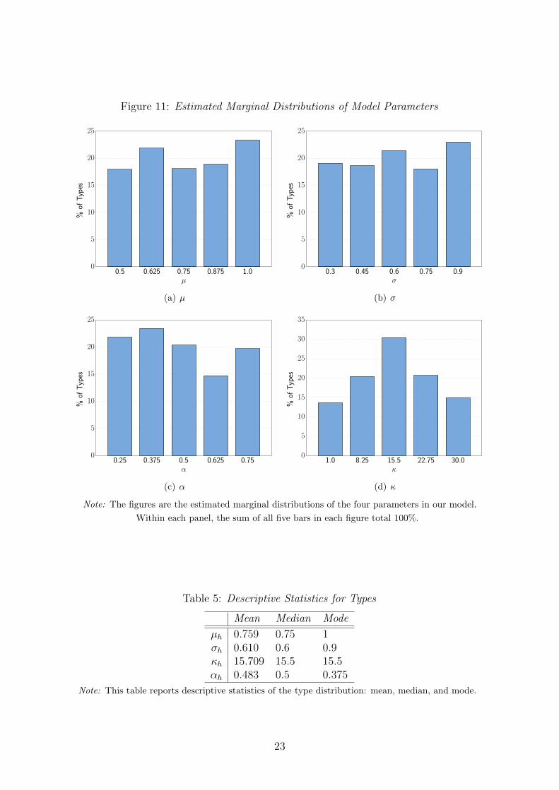
Figure 11: Estimated Marginal Distributions of Model Parameters

0.5 0.625 0.75 0.875 1.0µ

0

5

10

15

20

25

%of

Types

(a) µ

0.3 0.45 0.6 0.75 0.9σ

0

5

10

15

20

25

%of

Types

(b) σ

0.25 0.375 0.5 0.625 0.75α

0

5

10

15

20

25

%of

Types

(c) α

1.0 8.25 15.5 22.75 30.0κ

0

5

10

15

20

25

30

35

%of

Types

(d) κ

Note: The figures are the estimated marginal distributions of the four parameters in our model.

Within each panel, the sum of all five bars in each figure total 100%.

Table 5: Descriptive Statistics for Types

Mean Median Mode

µh 0.759 0.75 1σh 0.610 0.6 0.9κh 15.709 15.5 15.5αh 0.483 0.5 0.375

Note: This table reports descriptive statistics of the type distribution: mean, median, and mode.

23

ported in Table 5, are quite similar. For each of the parameters, the mean, median, and

mode are within 10% of one another.

The estimated joint distributions are much more irregular, neither uniform or nor-

mal. These joint distributions for each combination of the parameters, six in total, are

presented in Figure 12. Like Nevo et al. (2016), the joint distributions are multi-peaked

and vary considerably by the pair of parameters considered. This demonstrates the im-

portance of the flexibility of our estimation approach, which allows for free correlations

between each pair of parameters rather than the zero covariance often assumed in struc-

tural econometric applications. This flexibility is reflected in the fit of the model. For all

plans, the correlation between the empirical moments and the fitted moments is above

90%. The model also fits patterns in the data not explicitly used in estimation, similar

to those reported in Nevo et al. (2016).

5.2 Value of Eliminating Congestion

In this counterfactual exercise, we measure the value to subscribers from eliminating

network congestion, or the case where provisioned speeds are always realized to sub-

scribers. This exercise is import because it illustrates the value, or lack thereof, of many

types of core network improvements that go towards reducing congestion and better

meeting demand.

By eliminating congestion, we estimate an increase in consumer surplus of 14%, as

shown in Table 6. Daily usage increases from 2.2 GB/day to 2.5 GB/day, or about an

additional 9 GB over a 30-day billing cycle. We also observe many subscribers down-

grading plans as a result of the improved network state. Since the speeds of a cheaper

plan are now guaranteed, subscribers with a stronger preference for speed over usage may

be better served on the cheaper plan. This movement to cheaper plans lowers average

revenue for the ISP, but the increase in consumer surplus is large enough to offset this

drop: $4.24 drop in revenue and $8.90 increase in consumer surplus for a net difference of

$4.66. Since subscribers are receiving speeds roughly 19% faster, we estimate a subscriber

values each additional Mbps of realized speed at $2.87.

6 ConclusionWe estimate demand for residential broadband using a 10-month panel of hourly sub-

scriber usage and network conditions. The key feature of our model is the incorporation of

network congestion and allowing it to affect a subscriber’s daily consumption decision.19

There are three sources of variation we exploit in our data. First, we use (shadow) price

variation that results from the structure of usage-based pricing’s three-part tariff. Sec-

ond, we use cross-sectional variation in packet loss, our measure of network congestion,

19This differs from previous research such as Nevo et al. (2016).

24

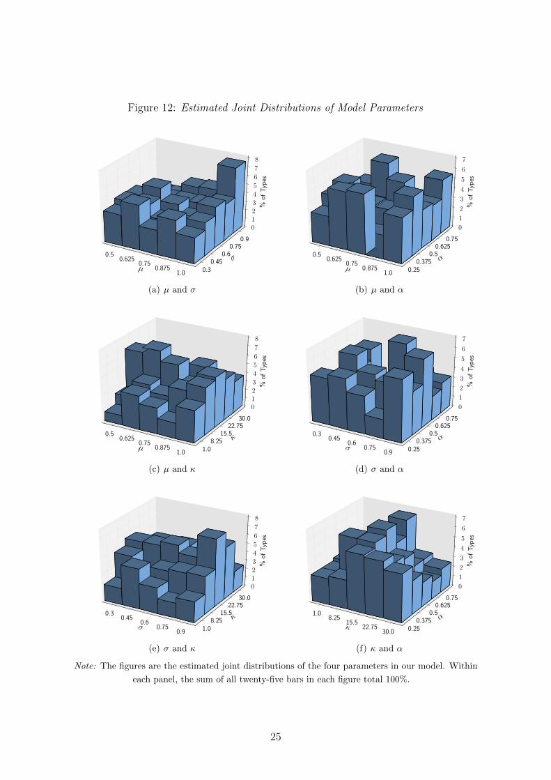
Figure 12: Estimated Joint Distributions of Model Parameters

µ

0.50.625

0.750.875

1.0

σ

0.30.45

0.60.75

0.9

%of

Types

01234

5

6

7

8

(a) µ and σ

µ

0.50.625

0.750.875

1.0

α0.25

0.3750.50.625

0.75

%of

Types

0

1

2

3

4

5

6

7

(b) µ and α

µ

0.50.625

0.750.875

1.0

κ

1.08.25

15.522.75

30.0

%of

Types

01234

5

6

7

8

(c) µ and κ

σ

0.30.45

0.60.75

0.9

α0.25

0.3750.50.625

0.75

%of

Types

0

1

2

3

4

5

6

7

(d) σ and α

σ

0.30.45

0.60.75

0.9

κ

1.08.25

15.522.75

30.0

%of

Types

01234

5

6

7

8

(e) σ and κ

κ

1.08.25

15.522.75

30.0

α0.25

0.3750.50.625

0.75

%of

Types

0

1

2

3

4

5

6

7

(f) κ and α

Note: The figures are the estimated joint distributions of the four parameters in our model. Within

each panel, the sum of all twenty-five bars in each figure total 100%.

25

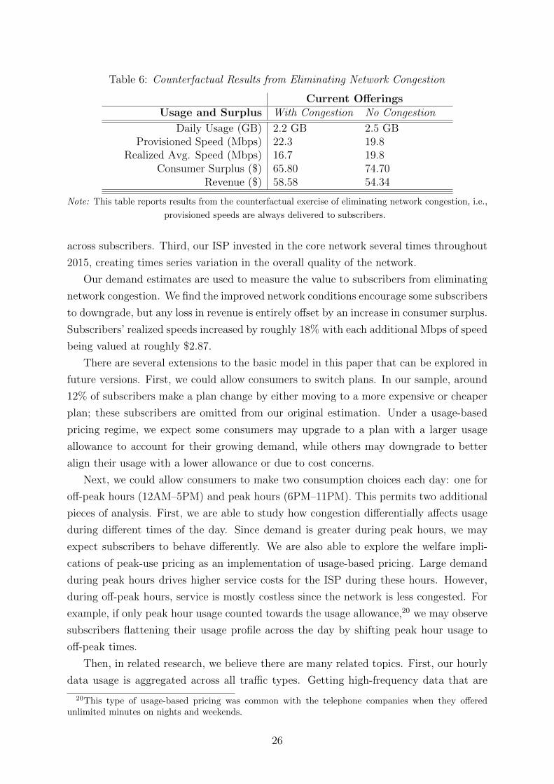
Table 6: Counterfactual Results from Eliminating Network Congestion

Current OfferingsUsage and Surplus With Congestion No Congestion

Daily Usage (GB) 2.2 GB 2.5 GBProvisioned Speed (Mbps) 22.3 19.8

Realized Avg. Speed (Mbps) 16.7 19.8Consumer Surplus ($) 65.80 74.70

Revenue ($) 58.58 54.34

Note: This table reports results from the counterfactual exercise of eliminating network congestion, i.e.,

provisioned speeds are always delivered to subscribers.

across subscribers. Third, our ISP invested in the core network several times throughout

2015, creating times series variation in the overall quality of the network.

Our demand estimates are used to measure the value to subscribers from eliminating

network congestion. We find the improved network conditions encourage some subscribers

to downgrade, but any loss in revenue is entirely offset by an increase in consumer surplus.

Subscribers’ realized speeds increased by roughly 18% with each additional Mbps of speed

being valued at roughly $2.87.

There are several extensions to the basic model in this paper that can be explored in

future versions. First, we could allow consumers to switch plans. In our sample, around

12% of subscribers make a plan change by either moving to a more expensive or cheaper

plan; these subscribers are omitted from our original estimation. Under a usage-based

pricing regime, we expect some consumers may upgrade to a plan with a larger usage

allowance to account for their growing demand, while others may downgrade to better

align their usage with a lower allowance or due to cost concerns.

Next, we could allow consumers to make two consumption choices each day: one for

off-peak hours (12AM–5PM) and peak hours (6PM–11PM). This permits two additional

pieces of analysis. First, we are able to study how congestion differentially affects usage

during different times of the day. Since demand is greater during peak hours, we may

expect subscribers to behave differently. We are also able to explore the welfare impli-

cations of peak-use pricing as an implementation of usage-based pricing. Large demand

during peak hours drives higher service costs for the ISP during these hours. However,

during off-peak hours, service is mostly costless since the network is less congested. For

example, if only peak hour usage counted towards the usage allowance,20 we may observe

subscribers flattening their usage profile across the day by shifting peak hour usage to

off-peak times.

Then, in related research, we believe there are many related topics. First, our hourly

data usage is aggregated across all traffic types. Getting high-frequency data that are

20This type of usage-based pricing was common with the telephone companies when they offeredunlimited minutes on nights and weekends.

26

disaggregated by application or traffic type would permit a more detailed analysis and

understanding of how congestion differentially affects each type. Moreover, moving to

a move granular level, say 5 to 15 minutes, would allow for a more exact understand-

ing of the correlation between usage and congestion. Second, residential broadband and

traditional linear television (TV) services are closely related and are often bundled to-

gether by ISPs. In future research, we hope to obtain linear TV data in conjunction with

disaggregated high-frequency Internet usage by type to more completely explore how sub-

scribers use broadband Internet. Specific relationships like the substitutability of linear

TV and over-the-top video (OTTV) and how linear TV usage and network congestion

are correlated could be explored with such a data set.

ReferencesDutz, Mark, Jonathan Orszag and Robert Willig (2009). “The Substantial Consumber

Benefits of Broadband Connectivity for US Households.” Internet Intervention Alliance

Working Paper.

Edell, Richard and Pravin Varaiya (2002). Providing Internet Access: What We Learn

from INDEX, volume Broadband: Should We Regulate High-Speed Internet Access?

Brookings Institution.

Goolsbee, Austan and Peter Klenow (2006). “Valuing Products by the Time Spent Using

Them: An Application to the Internet.” American Economic Review P&P, 96(2): 108–

113.

Greenstein, Shane and Ryan McDevitt (2011). “The Broadband Bonus: Estimating

Broadband Internet’s Economic Value.” Telecommunications Policy, 35(7): 617–632.

Hitte, Loran and Prasanna Tambe (2007). “Broadband Adoption and Content Consump-

tion.” Information Economics and Policy, 74(6): 1637–1673.

Lambrecht, Anja, Katja Seim and Bernd Skiera (2007). “Does Uncertainty Matter? Con-

sumer Behavior Under Three-Part Tariffs.” Marketing Science, 26(5): 698–710.

Malone, Jacob, Aviv Nevo and Jonathan Williams (2016). “A Snapshot of the Current

State of Residential Broadband Networks.” NET Institute Working Paper No. 15-06.

Malone, Jacob, John Turner and Jonathan Williams (2014). “Do Three-Part Tariffs Im-

prove Efficiency in Residential Broadband Networks?” Telecommunications Policy,

38(11): 1035–1045.

Nevo, Aviv, John Turner and Jonathan Williams (2016). “Usage-Based Pricing and De-

mand for Residential Broadband.” Econometrica, 84(2): 411–443.

27

Rosston, Gregory, Scott Savage and Bradley Wimmer (2013). “Effect of Network Un-

bundling on Retail Price: Evidence from the Telecommunications Act of 1996.” Journal

of Law and Economics, 56(2): 487–519.

Varian, Hal (2002). The Demand for Bandwidth: Evidence from the INDEX Experiment,

volume Broadband: Should We Regulate High-Speed Internet Access? Brookings In-

stitution.

28