THE TRADE-OFF BETWEEN CHILD QUANTITY AND CHILD QUALITY … · Objektif makalah ini ialah untuk mengkaji sama ada teori timbal ... to a decrease in the marginal cost of child quality

61

Malaysian Management Journal Vol. 14, 61–71 (2010)

THE TRADE-OFF BETWEEN CHILD QUANTITY AND CHILD QUALITY AND THE PUBLIC PROVISION OF EDUCATION:

A CASE STUDY IN RURAL TERENGGANU, MALAYSIA

NOR AZAM ABDUL RAZAK ROSLAN ABDUL HAKIM

RUSSAYANI ISMAILUUM College of BusinessUniversiti Utara Malaysia

Abstract

The objective of this paper is to examine whether the theory of the child quantity-quality (CQQ) trade-off developed by Becker and Lewis (1973) is borne out by the data from a developing country. In brief, the theory states that households behave differently with respect to their mixture of child quantity and child quality depending on their standards of living (i.e. low-income households tend to choose child quantity at the expense of child quality, and the converse is true for high-income households). If the government provides enough support for education, however, this trade-off might be undermined. Using a sample of 885 children from a survey of 2,500 households in rural areas in Terengganu in 2009, we conducted an empirical analysis on the relationship between child quantity and child quality. In the baseline estimation as well as in a series of robustness check, our key findings are that there is a positive yet insignificant impact of child quantity on child quality. Accordingly, we take these results as mild evidence against the CQQ trade-off which, in turn, can be attributed to the magnitude of the public provision of education in Malaysia.

Keywords: Child quantity, child quality, CQQ trade-off, public provision of education.

Abstrak

Objektif makalah ini ialah untuk mengkaji sama ada teori timbal balik antara kuantiti anak dengan kualiti anak (CQQ) yang diketengahkan oleh Becker dan Lewis (1973) disokong oleh data daripada sebuah negara membangun. Secara ringkasnya, teori ini menyatakan bahawa gelagat isi rumah adalah berbeza dari segi kombinasi kuantiti anak dan kualiti anak bergantung kepada taraf hidup mereka (isi rumah berpendapatan rendah lebih cenderung kepada anak yang ramai berbanding kualiti manakala isi rumah berpendapatan tinggi lebih gemar kepada anak yang berkualiti berbanding jumlah). Namun begitu, jika kerajaan memberikan sokongan yang mencukupi dalam bidang pendidikan, timbal balik ini mungkin menjadi lemah. Dengan menggunakan sampel 885 anak-anak daripada satu kajian terhadap 2,500 isi rumah di kawasan pedalaman di Terengganu pada tahun 2009, penyelidik menjalankan satu kajian empirik tentang hubungan antara kuantiti anak dan kualiti anak. Dalam penganggaran asas dan lanjutan, dapatan utama kajian ini ialah kuantiti anak mempunyai kesan positif tetapi tidak signifikan terhadap kualiti anak. Oleh itu, penyelidik menginterpretasikan dapatan kajian ini sebagai bukti yang agak lemah

http

://m

mj.u

um.e

du.m

y

62


Introduction

Human capital is vital in promoting economic growth and development of a country. This is because human capital, defined as knowledge and skills embodied in persons, enables workers to be more productive and innovative, both of which serve as basic ingredients of economic growth. Accordingly, it is imperative that a country’s development policy include human capital accumulation as one of its main agenda. In this respect, it appears that the decision of households with regard to fertility has an important consequence on the future stock of human capital of a nation. Specifically, if a household chooses to have many children, then the children tend to be relatively uneducated. Conversely, if a household chooses to have few children, then the children tend to be relatively educated. As a consequence, a society which is characterized by a disproportionately huge share of large families is expected to produce a greater stock of future human capital than a society characterized by a greater share of large families. What could have accounted for the discrepancy in the behaviour of these households?

In a pioneering work, Becker and Lewis (1973) hypothesize that the trade-off between child quantity and child quality is dictated by the level of household income. In particular, low-income households tend to have relatively many, yet uneducated children while high-income households tend to have relatively few, yet educated children. In order to explain why changes in household income generate the trade-off, Becker and Lewis (1973) offer three key propositions. First, the marginal cost of child quantity (i.e. the additional cost associated with raising one more child) is an increasing function of child quality.1 Second, the marginal cost of

terhadap penolakan teori timbal balik CQQ. Penolakan teori ini mungkin boleh dikaitkan dengan tahap sumbangan awam yang besar dalam bidang pendidikan.

Kata kunci: Kuantiti anak, kualiti anak, timbal balik CQQ, sumbangan awam pendidikan.

child quality (i.e. the additional cost associated with upgrading the existing children’s education) is an increasing function of child quantity.2 Third, provided that the demand for each child quantity and child quality is an increasing function of household income, the income elasticity of demand for child quality is much larger than the income elasticity of demand for child quantity.3,4 This means that households tend to respond more positively to child quality than child quantity as their incomes rise.

For simplicity, assume that the income elasticity of demand for child quality is positive while the income elasticity of demand for child quantity is zero. Then, an increase in household income is expected to raise child quality while leaving child quantity unchanged. The increase in child quality is then expected to raise the marginal cost of child quantity (since the marginal cost of child quantity is a positive function of child quality), which leads to a decrease in child quantity (since its marginal cost has risen), which leads to a decrease in the marginal cost of child quality (since the marginal cost of child quality is a positive function of child quality), which leads to a subsequent increase in child quality (since its marginal cost has fallen), and the process continues. The net effect of a rise in household income is to increase child quality and decrease child quantity; hence, the CQQ trade-off.

Following Becker and Lewis (1973), numerous empirical studies have been conducted to investigate whether child quantity exerts a negative impact on child quality. In most of these early studies, however, it was found that child quantity has a negative effect on child quality, thus lending support to the theory [see Blake (1989) for a survey of these studies]. In recent years, however, some influential studies such

http

://m

mj.u

um.e

du.m

y

63


as Black, Devereux and Salvanes (2005) and Angrist, Lavy and Schlosser (2010) have found that there is lack of evidence of the CQQ trade-off. The discrepancy between these findings, some argue, could be attributed to the problem of endogeneity. In particular, the older studies treat child quantity as an exogenous variable whereas the newer studies treat child quantity as an endogenous variable. [An important exception is an early study by Rosenzweig and Wolpin (1980).] From the theoretical point of view, child quantity is an endogenous variable since households choose both the quantity and quality of their children. As such, the results of these newer studies should be given more weight.

In another recent study, however, Li, Zhang and Zhu (2008) found that there is a trade-off even after tackling the problem of endogeneity. According to these scholars, the discrepancy between their results and those of Black, et al. (2005) and Angrist, et al. (2010) could be attributed to the extent of public provision of education. In the case of China, they argue, there is a poor provision of public education, thus parents have to bear the bulk of their children’s education costs. Consequently, the CQQ trade-off is dominant in the case of China. In light of this argument, this paper revisits the issue by specifically examining whether Li et al. (2008)’s argument holds in the case of Malaysia. Since education is highly subsidized in Malaysia, we expect little or no CQQ trade-off in the country.

Model Specification

Following the literature, we specify child quality (measured by child’s educational attainment) as a function of child quantity (or fertility) and a host of household characteristics as control variables. In view of its endogeneity, child quantity needs to be instrumented by an appropriate instrumental variable. A natural candidate for the instrument, as suggested by the empirical literature, is some exogenous variation in fertility (i.e. a variation in fertility that is exogenous to the choice of child quality but is correlated with the choice of child quantity). Hitherto, two frequently

used exogenous variations in fertility are the occurrence of twins (defined as a dummy variable which is equal to 1 if the nth birth is a twin and 0 otherwise) and gender sameness (defined as a dummy variable which is equal to 1 if the first nth children are of the same gender and 0 otherwise). The basis for their choice is two-fold. First, it is plausible to assume (and even confirm) that each of the candidate instruments is correlated with child quantity. Second, it is reasonable to argue that each of the candidate instruments is uncorrelated with child quality (except through child quantity) since it is unlikely that parents would underinvest in the education of their children simply because they are endowed with twin children or children of the same gender.

In the studies conducted by Black et al. (2005) and Li, et al. (2008), twins have been employed as the instrument. It is imperative therefore, that the present study employ the same variable. Since data on twins are not available in our data set, this study opts for gender sameness as the instrument for child quantity. This variable has been employed by Angrist and Evans (1988) and Conley and Glauber (2006), among others. Accordingly, our model can be specified as follows:

(1) (2)

where Educi is child i’s educational attainment (measured by the number of years of schooling), Kids is child quantity (i.e. the total number of children in a household), Sameness is a dummy variable for gender sameness (which is equal to 1 if the first two children are of the same gender and 0 otherwise), and x is a vector of control variables which include a child’s characteristics (i.e. gender, birth order, and age) and parents’ characteristics (i.e. parents’ age and parents’ education).

A priori, we expect the coefficient of Kids to be negative to reflect the adverse relationship between child quantity and child quality. In contrast, we expect the coefficient of Sameness to be positive to reflect parents’ preferences for children of mixed gender.

http

://m

mj.u

um.e

du.m

y

64


Data

The data in this study are obtained from an interview-based survey conducted on a sample of 2,500 rural households in Terengganu, Malaysia, in May 2009. Since the rural region of Terengganu is predominantly occupied by Malays, it is hardly surprising that all of the interviewed households are Malays. Since the unit of analysis is children (instead of households), we extracted the children data from these households. From the 2,500 households, the total number of children was 12,321 persons. This means that, on average, there are about five children per household.

One of the remarkable features of the empirical work on the CQQ trade-off is that the sample is subject to a number of restrictions. First, the sample needs to be restricted to school-aged children who are currently residing with their parents. This is usually accomplished by restricting the sample to children aged 5-17 or 6-17 [see Conley & Glauber (2006) and Li et al. (2008), respectively]. In the case of Malaysia, children begin schooling at the age of 7, and they are not so eager to leave their parents’ home once they graduate from high school. Hence, the children’s age-range can be expanded to, say, 7-20. Doing so reduces our sample size to

4,760 observations (i.e. a reduction of 7,561 observations).

Second, depending on the way the instrument for child quantity is defined, the sample needs to be restricted further. If gender sameness of the first two-born children is chosen as the instrument, then the sample needs to be restricted to households who have at least three children. Doing so decreases our sample size to 4,569 observations (i.e. a decline of 191 observations).

Third, given the instrument, too, the unit of analysis needs to be confined to the first two-born children. Doing so results in a huge drop in our sample size (i.e. by 3,374 observations), leaving us with 1,195 observations [see Black et al. (2005) and Conley & Glauber (2006) for the second and third sample restrictions].

Finally, the data for some of the variables of interest in this curtailed sample are either not available or suspicious. These missing and dubious values, in turn, shrink the sample size further by 310 observations. Hence, we end up with 885 observations. This figure corresponds to 430 households, all of whom are characterized by dual parents, 311 of whom (or 72%) are characterized by dual income earners, and 230 of whom (or 53%) are endowed with the first two-born children of the same gender.

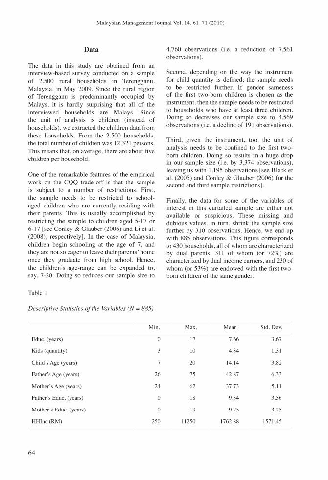
Table 1

Descriptive Statistics of the Variables (N = 885)

Min. Max. Mean Std. Dev.

Educ. (years) 0 17 7.66 3.67

Kids (quantity) 3 10 4.34 1.31

Child’s Age (years) 7 20 14.14 3.82

Father’s Age (years) 26 75 42.87 6.33

Mother’s Age (years) 24 62 37.73 5.11

Father’s Educ. (years) 0 18 9.34 3.56

Mother’s Educ. (years) 0 19 9.25 3.25

HHInc (RM) 250 11250 1762.88 1571.45

http

://m

mj.u

um.e

du.m

y

65


Given this substantially reduced sample size, the summary statistics of the key variables are as follows: Educ (i.e. children’s educational attainment) ranges from 0 to 17 years with the average of about 7.7 years, Kids (i.e. the number of children) ranges from 3 to 10 children with the average of about 4 children, age of the children ranges from 7 to 20 years with the average of about 14 years, 458 of the children (or 52%) are males, father’s age ranges from 26 to 75 years with the average of about 43 years, mother’s age ranges from 24 to 62 years with the average of about 38 years, father’s educational attainment ranges from 0 to 18 years with the average of about 9 years, and mother’s educational attainment ranges from 0 to 19 years with the average of about 9 years, and HHInc (i.e. household income) ranges from RM250 to RM11,250 with the average of about RM1,763 (see Table 1 for a more detailed summary of the tatistics of all of these variables).

Estimation Results

Given the necessary data for a sample of 885 children in Terengganu, Malaysia, we estimate Eq.(1) by the instrumental variable (IV) method, where Kids (i.e. child quantity) is instrumented by Sameness (i.e. gender sameness of the first two-born children), and Eq.(2) by the ordinary least squares (OLS) method. In other words, Eq.(2) serves as the first-stage regression and Eq.(1) the second-stage regression.

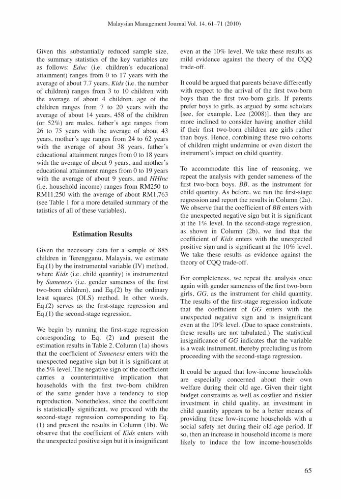
We begin by running the first-stage regression corresponding to Eq. (2) and present the estimation results in Table 2. Column (1a) shows that the coefficient of Sameness enters with the unexpected negative sign but it is significant at the 5% level. The negative sign of the coefficient carries a counterintuitive implication that households with the first two-born children of the same gender have a tendency to stop reproduction. Nonetheless, since the coefficient is statistically significant, we proceed with the second-stage regression corresponding to Eq. (1) and present the results in Column (1b). We observe that the coefficient of Kids enters with the unexpected positive sign but it is insignificant

even at the 10% level. We take these results as mild evidence against the theory of the CQQ trade-off.

It could be argued that parents behave differently with respect to the arrival of the first two-born boys than the first two-born girls. If parents prefer boys to girls, as argued by some scholars [see, for example, Lee (2008)], then they are more inclined to consider having another child if their first two-born children are girls rather than boys. Hence, combining these two cohorts of children might undermine or even distort the instrument’s impact on child quantity.

To accommodate this line of reasoning, we repeat the analysis with gender sameness of the first two-born boys, BB, as the instrument for child quantity. As before, we run the first-stage regression and report the results in Column (2a). We observe that the coefficient of BB enters with the unexpected negative sign but it is significant at the 1% level. In the second-stage regression, as shown in Column (2b), we find that the coefficient of Kids enters with the unexpected positive sign and is significant at the 10% level. We take these results as evidence against the theory of CQQ trade-off.

For completeness, we repeat the analysis once again with gender sameness of the first two-born girls, GG, as the instrument for child quantity. The results of the first-stage regression indicate that the coefficient of GG enters with the unexpected negative sign and is insignificant even at the 10% level. (Due to space constraints, these results are not tabulated.) The statistical insignificance of GG indicates that the variable is a weak instrument, thereby precluding us from proceeding with the second-stage regression.

It could be argued that low-income households are especially concerned about their own welfare during their old age. Given their tight budget constraints as well as costlier and riskier investment in child quality, an investment in child quantity appears to be a better means of providing these low-income households with a social safety net during their old-age period. If so, then an increase in household income is more likely to induce the low income-households

http

://m

mj.u

um.e

du.m

y

66


to have more children (instead of educated children). This implies that the trade-off between

Given this argument, a dummy variable representing low-income households needs to be introduced into our model. Recall from Table 1 that the average household income is

child quantity and child quality is unlikely to be applicable to low-income households.

Table 2

Baseline Estimation Results (N = 885)

(1a) (1b) (2a) (2b)

Dependent Variable Kids Educ. Kids Educ.

Constant 3.235***(9.25)

-8.600***(-3.90)

3.118***(8.99)

-10.358***(-5.10)

Kids - 0.553(0.81)

- 1.111*(1.80)

Sameness -0.163**(-2.07)

- - -

BB - - -0.301***(-2.77)

-

Child’s Gender -0.122(-1.54)

-0.032(-0.23)

0.037(0.38)

0.038(0.24)

Second Child 0.427***(5.18)

-0.233(-0.74)

0 .432***(5.25)

-0.472(-1.58)

Child’s Age 0.187***(13.39)

0.741***(5.74)

0.186***(13.33)

0.636***(5.40)

Father’s Age 0.009(1.00)

0.024*(1.65)

0.010(1.09)

0.019(1.13)

Mother’s Age -0.061***(-4.97)

0.046(1.01)

-0.061*(-4.95)

0.080*(1.85)

Father’s Educ. 0.026*(1.92)

0.036(1.40)

0.026*(1.96)

0.022(0.78)

Mother’s Educ. 0.006(0.43)

0.045**(2.15)

0.005(0.37)

0.042*(1.66)

Adj. R2 0.20 0.80 0.21 0.71

Note: Estimation is done by the IV method; columns (a) and (b) report the results from the first- and second-stage regressions, respectively. The figures in parentheses are t-values; ***, **, and * denote statistical significance at the 1%, 5%, and 10% levels, respectively.

about RM1,763 per month and the average quantity of children in each household is 4.34 persons, yielding the average household income per capita of about RM406 per month. Thus,

http

://m

mj.u

um.e

du.m

y

67


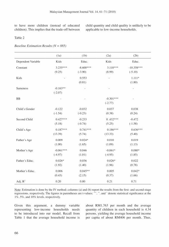
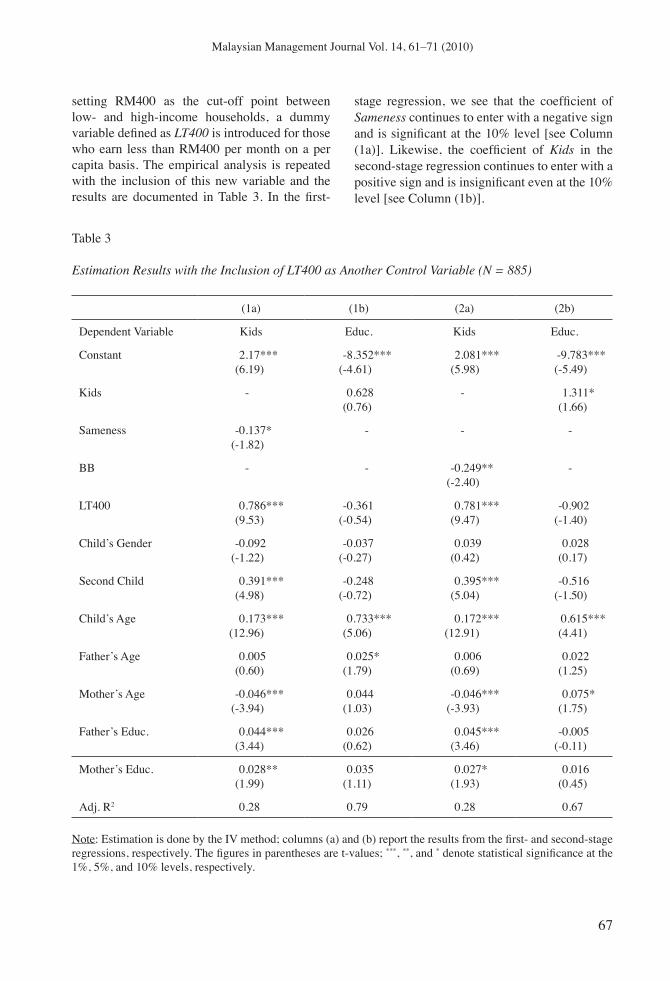
setting RM400 as the cut-off point between low- and high-income households, a dummy variable defined as LT400 is introduced for those who earn less than RM400 per month on a per capita basis. The empirical analysis is repeated with the inclusion of this new variable and the results are documented in Table 3. In the first-

stage regression, we see that the coefficient of Sameness continues to enter with a negative sign and is significant at the 10% level [see Column (1a)]. Likewise, the coefficient of Kids in the second-stage regression continues to enter with a positive sign and is insignificant even at the 10% level [see Column (1b)].

Table 3

Estimation Results with the Inclusion of LT400 as Another Control Variable (N = 885)

(1a) (1b) (2a) (2b)


Constant 2.17*** (6.19)

-8.352*** (-4.61)

2.081*** (5.98)

-9.783*** (-5.49)

Kids - 0.628 (0.76)

- 1.311* (1.66)

Sameness -0.137* (-1.82)

- - -

BB - - -0.249** (-2.40)

-

LT400 0.786*** (9.53)

-0.361 (-0.54)

0.781*** (9.47)

-0.902 (-1.40)

Child’s Gender -0.092 (-1.22)

-0.037 (-0.27)

0.039 (0.42)

0.028 (0.17)


-0.248 (-0.72)

0.395*** (5.04)

-0.516 (-1.50)

Child’s Age 0.173*** (12.96)

0.733*** (5.06)

0.172*** (12.91)

0.615*** (4.41)

Father’s Age 0.005 (0.60)

0.025* (1.79)

0.006 (0.69)

0.022 (1.25)

Mother’s Age -0.046*** (-3.94)

0.044 (1.03)

-0.046*** (-3.93)

0.075* (1.75)

Father’s Educ. 0.044*** (3.44)

0.026 (0.62)

0.045*** (3.46)

-0.005 (-0.11)

Mother’s Educ. 0.028** (1.99)

0.035 (1.11)

0.027* (1.93)

0.016 (0.45)

Adj. R2 0.28 0.79 0.28 0.67


http

://m

mj.u

um.e

du.m

y

68


As before, we repeat the analysis with BB as the instrument for child quantity in lieu of Sameness. As shown in Columns (2a) and (2b), the coefficients of interest (i.e. those of BB and Kids in the first- and second-stage regressions, respectively) enter with the same signs and significance levels as their counterparts in the baseline analysis. Finally, the analysis is repeated with GG as the instrument for child quantity. As before, we find that the coefficient of GG enters

with a negative sign and is insignificant. (Due to space constraints, these results are not tabulated.) Taken together, all of these results suggest that conditioning our analysis to low-income households does not affect the trade-off (or lack of it) between child quantity and child quality.

It could be argued that low-income households are not particularly concerned about the gender of the first two-born children. In order to provide

Table 4

Estimation Results with the Inclusion of LT400 as Another Instrument (N = 885)

(1a) (1b) (2a) (2b)


Constant 2.172*** (6.19)

-7.446*** (-11.61)

2.081*** (5.98)

-7.607*** (-11.87)

Kids - 0.187 (1.31)

- 0.238* (1.68)

Sameness -0.137* (-1.82)

- - -

BB - - -0.249** (-2.40)

-

LT400 0.786*** (9.53)

- 0.781*** (9.47)

-

Child’s Gender -0.092 (-1.22)

-0.078 (-0.74)

0.039 (0.42)

-0.072(-0.67)


-0.076 (-0.61)

0.395*** (5.04)

-0.098(-0.78)

Child’s Age 0.173*** (12.96)

0.809*** (24.99)

0.172*** (12.91)

0.800*** (24.78)

Father’s Age 0.005 (0.60)

0.027** (2.21)

0.006 (0.69)

0.027** (2.17)

Mother’s Age -0.046*** (-3.94)

0.023 (1.27)

-0.046*** (-3.93)

0.026 (1.43)

Father’s Educ. 0.044*** (3.44)

0.046** (2.53)

0.045*** (3.46)

0.045** (2.45)

Mother’s Educ. 0.028** (1.99)

0.048** (2.47)

0.027* (1.93)

0.047** (2.44)

Adj. R2 0.28 0.82 0.28 0.82


http

://m

mj.u

um.e

du.m

y

69


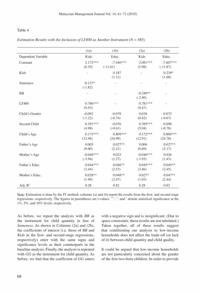
with a social safety net during their old age, these low-income households might continue to have more children regardless of the gender of the first two-born children. For non-poor households, however, the decision to have more children might depend upon the gender of the first two-born; i.e. they are more likely to add a third child if the first two-born are of the same gender. If so, then gender sameness is unlikely to be applicable to low-income households.

Given this conjecture, the dummy LT400 qualifies as an additional instrument for child quality. The empirical analysis is repeated with the inclusion of this additional dummy in the first-stage regression and the results are reported in Table 4. As shown in Column (1a), the coefficient of Sameness enters with a negative sign and is significant at the 10% level and the coefficient of LT400 enters with a positive sign and is significant at the 1% level. Since both coefficients are jointly significant at the 1% level, we proceed with the second-stage regression. As before, we observe that the coefficient of Kids enters with the unexpected positive sign and is insignificant [see Column (1b)].

Repeating the analysis with BB in place of Sameness, we see that the coefficient of BB enters with a negative sign and is significant at the 5% level and the coefficient of LT400 enters with a positive sign and is significant at the 1% level [see Column (2a)]. Again, since both coefficients are jointly significant at the 1% level, we proceed with the second-stage regression: now not only that the coefficient of Kids enters with the usual positive sign, it is also significant at the 10% level [see Column (2b)]. Finally, the analysis is repeated with GG in lieu of Sameness. As before, the coefficient of GG enters with the usual negative sign and is insignificant. However, the coefficient of LT400 enters with a positive sign and is significant at the 1% level. Since both coefficients are jointly significant at the 1% level, we proceed with the second-stage regression and find that the coefficient of Kids enters with a positive sign albeit insignificant. (Again, these results are not tabulated due to space constraints.) Here, the evidence is clear-

cut: regardless of which instrument is used, the results appear to be at odds with the CQQ trade-off theory. Overall, our empirical results indicate that there is a positive yet insignificant impact of child quantity on child quality, suggesting that there is mild evidence against the theory of CQQ trade-off.

Discussion

The premise of the CQQ trade-off (i.e. households behave differently with respect to their mixture of child quantity and child quality depending on their standards of living) carries a nuisance long-run implication. This is the case because if the premise holds, then we would expect to see a vicious cycle of child quantity-quality divide between low- and high-income households. To illustrate, consider the first generation of households. The poor households tend to produce relatively many yet uneducated children who will later become the second generation of poor households. In contrast, the rich households tend to produce relatively few yet educated children who will later become the second generation of rich households. Now consider the second generation of households. Compared to the first generation, the second generation of households tends to be more diverse in the sense that the poor tend to be disproportionately larger than the rich. The poor households tend to produce relatively many yet uneducated children who will later become the third generation of poor households. In contrast, the rich households tend to produce relatively few yet educated children who will later become the third generation of rich households. Needless to say, the third generation of households tends to be even more diverse in that the proportion of the poor outweighs that of the rich. For both poor and rich households, the cycle continues from one generation to the next, resulting in the ever-growing divergence in the household’s behaviour between low- and high-income households within a society.

If the vicious cycle of child quantity-quality divide persists over time, then the economic implication is extremely staggering; i.e. there is

http

://m

mj.u

um.e

du.m

y

70


an inherent tendency towards widening income inequality even for a society with a relatively balanced income distribution. Are we observing this phenomenon in the real world? Perhaps it is fair to say that this phenomenon is far from universal, and we would argue that this lack of universal phenomenon can be attributed to the public provision of education. If the government provides enough financial support for education, then poor households may not choose child quantity at the expense of child quality, thereby undermining the CQQ trade-off. To illustrate, note that human capital is accumulated through an investment in education from the primary level to the secondary and tertiary levels. Since educational investment is costly, and its cost increases with the level of education, the poor segment of the population is likely to be denied access to education, especially at the higher levels. In order to compensate this unfortunate segment of the society, the governments usually intervene by providing free and/or subsidized education to the poor. The degree of government intervention varies across countries, however. According to the Education for All Global Monitoring Report released by UNESCO (2011), the share of education in the total public expenditure in the world ranged from 7% to 27% in 2008, with the world average of 14% and that of Malaysia stood at 18%.

If the magnitude of the education share of the total public expenditure can be taken as an indicator of the extent to which the unfortunate segment of the population (i.e., the group of poor households) is being compensated, then it is possible to assess whether a given amount of the public provision of education is adequate. Consequently, testing the trade-off between child quantity and child quality can shed light on the issue of whether the public provision of education is adequate. If the test yields a result that lends support to the theory, then we conclude that there is inadequate public provision of education; otherwise, there is adequate public provision of education. In this paper, we obtain results that appear to be inconsistent with the theory. On the basis of these results, we conclude that there is adequate public provision of education in Malaysia.

Conclusion

In this paper, we revisit the issue of CQQ trade-off in the context of a rural area in a developing country, Malaysia. Using a sample of 885 children from rural areas in Terengganu, Malaysia, we conducted an empirical analysis of the relationship between child quantity and child quality based on the standard instrumental variable method. Our baseline findings indicate that the estimated coefficient of child quantity is positive but insignificant even at the 10% level. It appears that these results are broadly robust to the conditioning of our sample on low-income households, LT400, either as an additional control variable or as an additional instrument. Accordingly, we take all of these results as mild evidence against the CQQ trade-of theory. Our results appear to be consistent with those of Black et al. (2005), and Angrist, et al. (2010) but inconsistent with Li et al. (2008). Nevertheless, we agree with Li et al. (2008)’s argument that the trade-off between child quantity and child quality depends on the extent of public support for education. In the case of Malaysia, primary and secondary education is basically provided for free, and tertiary education is highly subsidized.

End Notes

1 To illustrate, consider two households, A and B, each of whom has the same number of children (say, 3) but A’s children are more educated. Then, adding another child is more costly for A. In other words, the marginal cost of child quantity is higher for A.2 To illustrate, consider two households, M and N, each of whom has children of the same level of education (say, 13 years of education) but M has more children than N. Then, adding another year of education is more costly for M. In other words, the marginal cost of child quality is higher for M.3 The income elasticity of demand for child quality (quantity) refers to the degree of responsiveness of the demand for child quality (quantity) with respect to a change in household income.

http

://m

mj.u

um.e

du.m

y

71


4 In a subsequent analysis, Becker and Tomes (1976) demonstrate that the third proposition can be interpreted as a result of the decomposition of child quality into two: endowed contribution to child quality (i.e. inherited ability) and household contribution to child quality (i.e. parental investment in child quality).

References

Angrist, J., & Evans, W. (1998). Children and their parent’s labor supply: Evidence from exogenous variation in family size. American Economic Review, 88, 450–477.

Angrist, J., Lavy, V., & Schlosser, V. (2010). Multiple experiments for the causal link between the quantity and quality of children. Journal of Labor Economics, 28, 773–823.

Becker, G., & Lewis, H. (1973). On the interaction between the quantity and quality of children. Journal of Political Economy, 81, S279–S288.

Becker, G., & Tomes, N. (1976). Child endowments and the quantity and quality of children. Journal of Political Economy, 84, S143–S162.

Black, S., Devereux, P., & Salvanes, K. (2005). The more the merrier? The effect of family size and birth order on children’s education. Quarterly Journal of Economics, 120, 669–700.

Blake, J. (1989). Family size and achievement. Berkeley and Los Angeles, CA: University of California Press.

Conley, D., & Glauber, R. (2006). Parental educational investment and children’s academic risk: Estimates of the impact of sibship size and birth order from exogenous variation in fertility. Journal of Human Resources, 41, 722–737.

Lee, J., (2008). Sibling size and investment in children’s education: An Asian instrument. Journal of Population Economics, 21, 855–875.

Li, H., Zhang, J., & Zhu, Y. (2008). The quantity-quality trade-off of children in a developing country: Identification using Chinese twins. Demography, 45, 223–243.

Rosenzweig, M., & Wolpin, K. (1980). Testing the quantity-quality fertility model: The use of twins as a natural experiment. Econometrica, 48, 227–240.

UNESCO. (2011). Education for All Global Monitoring Report. UNESCO.

http

://m

mj.u

um.e

du.m

y

Documents

THE TRADE-OFF BETWEEN CHILD QUANTITY AND CHILD QUALITY … · Objektif makalah ini ialah untuk mengkaji sama ada teori timbal ... to a decrease in the marginal cost of child quality