TECHNICAL REPORT CERC-84-7

THE TMA SHALLOW-WATER SPECTRUMDESCRIPTION AND APPLICATIONS

by

Steven A. Hughes

Coastal Engineering Research Center

DEPARTMENT OF THE ARMYWaterways Experiment Station, Corps of Engineers

IC PO Box 631, Vicksburg, Mississippi 39180-0631

H. too.

December 1984Final Report

Approved For Public Release; Distribution Unlimited

F-1-

Prepared for DEPARTMENT OF THE ARMY

US Army Corps of EngineersWashington, DC 20314-1000

Under Civil Works Research Work Unit 31592

06 6 O 0O

Destroy this report when no longer needed. Do not returnit to the originator.

The findings in this report are not to be construed as an officialDepartment of the Army position unless so designated

by other authorized documents.

The contents of this report are not to be used foradvertising, publication, or promotional purposes.Citation of trade names does not constitute anofficial endorsement or approval of the use of

such commercial products.J AL-OsSlon ForNTIS QRA&I

I TAB 0U. , i'j-)unce i

JuA ... cat. o

By-Distx' !)Ution/

Availability CodesAvail nnd/oz

Dist Special

UnclassifiedSECURITY CLASSIFICATION OF THIS PAGE (lWhen Date Entered)

REPORT DOCUMENTATION PAGE READ INSTRUCTIONSBEFORE COMPLETING FORM

I. REPORT NUMBER 2. GOVT ACC 3 ECPLNT'S CATALOG NUMBER

Technical Report CERC-84-7 zi

4. TITLE (and Subtitle) 3. TYPE OF REPORT & PERIOD COVERED

THE TMA SHALLOW-WATER SPECTRUM Final reportDESCRIPTION AND APPLICATIONS 6. PERFORMING ORG. REPORT NCMBER

7. AUTHOR(s) 8. CONTRACT OR GRANT NUMBER(&)

Steven A. Hughes

9. PERFORMING ORGANIZATION NAME AND ADDRESS 10. PROGRAM ELEMENT, PROJECT. TASK

US Army Engineer Waterways Experiment Station AREA A WORK UNIT NUMBERS

Coastal Engineering Research Center Civil Works Research Work

PO Box 631, Vicksburg, Mississippi 39180-0631 Unit 31592

1,. CONTROLLING OFFICE NAME AND ADDRESS 1,. REPORT DATEDEPARTMENT OF THE ARMY December 1984US Army Corps of Engineers 13. NUMBER OF PAGESWashington, DC 20314-1000 42

14. MONITORING AGENCY NAME & ADORESS(if diffeent from Controlling Office) 15. SECURITY CLASS. (4 this report)

Unclassified

IS&. OECL ASSI FIC ATION.'DOWNGRADINGSCHEDULE

IS. DISTRIBUTION STATEMENT (of this Report)

Approved for public release; distribution unlimited.

17. DISTRIBUTION STATEMENT (of the abetect entered In Block 20. if dillerent from Report)

1B. SUPPLEMENTARY NOTES

Available from National Technical Information Service, 5285 Port Royal Road,Springfield, Virginia 22161.

19. KEY WORDS (Continue on revered side it neceesary ad Identify by block number)

Parametric SpectrumSelf-similar WavesShallow-water wavesSimilarity

20. A9STRACT (Cmt ae a reverse eid Iffemeamn awd identy by block u mnbe

r)

Recent advances have been made in the specification of a shallow-waterself-similar spectral form. This spectral form, referred to as the ThA spec-trum, substitutes an expression for the shallow-water equilibrium range intothe JONSWAP equation for spectral energy density. The JONSWAP parameters areempirically defined through examination of over 2,800 wind sea spectra ob-tained at various depths and locations. This spectral form is intended to

(Continued)

D t mmOF I 6 S oSSOEr[ Unclassified

SECURITY CLASSIFICATION OF THIS PA E (rWhen Data Entered)

Iilirm~ I.O

UnclassifiedSECURITY CLASSIFICATION OF THIS PAGE(IIi Dia EAIR00,,

20. ABSTRACT (Continued).

_describe single-peaked wind seas which have reached a growth equilibrium in

finite depth water. The purposes of this report are to summarize the recent

advances, to discuss the range, of practical usage, and to provide engineering

examples using these new formulations.

UnclassifiedSECURITY CLASSIFICATION OF THIS PAGE(Inon Data ffnfered)

'i+ ,.-*' ? "+" .++. '' . ./

A+ [+.++ , ++ ' + + + + +.++ + +,,>-.

PREFACE

The developments described in this paper are primarily a result of

research conducted by an international group comprised of E. Bouws, Royal

Netherlands Meteorological Institute; H. Gunther and W. Rosenthal, University

of Hamburg and Max-Plank-Institut fur Meteorologie; and C. L. Vincent, Coastal

Engineering Research Center (CERC), US Army Engineer Waterways Experiment

Station (WES). Extensions of this basic work by C. L. Vincent and S. A.

Hughes are also included.

The research summarized in this report was authorized by the Office,

Chief of Engineers (OCE), US Army Corps of Engineers, under Civil Works Re-

search Work Unit 31592, "Wave Estimation for Design." Funds were provided

through the Coastal Engineering Research Area under the field management of

CERC and Mr. J. H. Lockhart, Jr., OCE Technical Monitor.

This report was written by Dr. Steven A. Hughes, Research Hydraulic

Engineer, under direct supervision of Dr. E. F. Thompson, Chief, Coastal

Oceanography Branch and under general supervision of Drs. J. R. Houston,

Chief, Research Division and R. W. Whalin, Chief, CERC.

1Commaoder and Director of WES during the publication of this report was

COL Robert C. Lee, CE. Technical Director was Mr. F. R. Brown.

,%-

°

CONTENTS

Page

PREFACE . . . . . . . . . . . . . . . . . . . . . . . . . . . . . . . . 1

PART I: INTRODUCTION ............ ........................ 3

PART II: SHALLOW-WATER DEVELOPMENTS ......... ................. 6

Equilibrium Range ............ ........................ 6Depth-Limited Significant Wave Height ....... .............. 8TKA Spectrum .......... ........................... 9Wave Growth Limitation ....... ..................... . 15

PART III: SURF ZONE SPECTRA ........... ..................... 19

Fit of TMA to Collected Spectra ..... ................. . 19Hypothesis for Energy Saturation ..... ................ . 20

PART IV: DISCUSSION ......... ......................... ... 27

Physical Implications of the TMA Spectral Form .......... . 27Assumptions and Limitations of the TMA Spectral Form ...... . 28

PART V: ENGINEERING APPLICATIONS ...... .................. . 30

Numerical Models ........ ........................ . 30Design Example 1 ........ ........................ . 30Design Example 2 ......... ........................ . 32Design Example 3 ......... ........................ . 34Design Example 4 ......... ........................ . 35

PART VI: SUMMARY .......... .......................... . 37

REFERENCES ............ .............................. .. 38

APPENDIX A: NOTATION ............ ......................... Al

4i%

% 2

." THE ThA SHALLOW-WATER SPECTRUM

DESCRIPTION AND APPLICATIONS

PART I: INTRODUCTION

1. Determination of realistic estimates for wave conditions in shallow

water has always been important in coastal engineering. Initially monochro-

matic wave theory was used exclusively, but it is .ow generally accepted that

an irregular wave approach is preferred. The purposes of this report are to

summarize recent advances in the specification of a shallow-water self-similar

spectral form, to discuss the range of practical usage, and to provide engi-

neering examples using the new formulations.

2. The first quantitative predictions of ocean waves evolved from ob-

servations of waves at a point in space and correlations between such parame-

ters as mean wave height, significant wave height, and mean wave period. In

the mid-1950's the spectral description of the sea state was forwarded. This

description allowed for more detail by distinguishing between the different

frequency bands. Phillips (1958) suggested that there should be a region of

the spectrum of wind-generated deepwater gravity waves in which the wave

energy density has an upper bound given by the following expression:

Em (f) = ag2 f -5(2n)-4 (1)mm

where f is frequency,* g is gravitational acceleration, and a was as-

-3sumed to be a universal constant, approximately 8 X 10 . This region of the

spectrum is called the equilibrium range. In scalar wave number space this

equilibrium range becomes

F(k) = - (2)

where P is a constant and k is the wave number equal to 2n/L when L is

the wave length. The limit, defined by Equation I or 2, was thought to be a

* For convenience, symbols and abbreviations are listed in the Notation

(Appendix A).

3

result of a limiting wave steepness at each frequency beyond which deepwater

wave breaking would occur. In other words, any additional energy input in the

spectrum at that frequency would result in waves breaking and a transfer of

wave energy from that frequency through the mechanisms of dissipation and

wave-wave interactions. This represents the equilibrium or steady-state wind

sea situation in deep water, and Equation 1 describes the portion of the spec-

* trum to the high frequency side of the single spectral peak.

3. A spectral shape for fully developed deepwater waves was advanced by

Pierson and Moskowitz (1964) containing Phillips' equilibrium range

* .. (Equation 1). It is expressed as

E mM mM -5/4(f/fM) -4(3Epm(f)=E E(f)e m(3)

where f is the frequency of the spectral peak. The additional exponentialm

term provides the low frequency forward face of the spectrum and a broad,

smooth peak region. Equation 3 is based on extensive field data. Estimation

of f for fully developed seas (i.e., no further wave growth could occur atm

that windspeed) was empirically determined in terms of 10-m-high windspeed U

as

f = 0.82 (4). %m 2nrU

Integration of Equation 3 provides the total energy E in the spectrum.

Longuet-Higgins (1952) has shown that 4 times the variance, or 4(E) 1/ 2 , pro-

vides a close estimate of significant wave height in deep water. Thus a

method exists for hindcasting and forecasting fully developed deepwater wave

heights and periods.

4. One drawback to the fully developed representation was that at

higher windspeeds the wind seldom held steady for the length of time necessary

for fully saturated seas to develop. In other cases the fetch over which the

wind acted wasn't long enough for fully developed conditions.

5. The data from the Joint North Sea Wave Program (JONSWAP) were used

by Hasselmann, et al. (1973) to extend the Pierson-Moskowitz spectral density

representation (Equation 3) to partially developed wave conditions by the ad-

dition of another factor:

4

W-~~~~ ~~ _- - .. nn~.~.------- .-p- .- 5/4(f/f ) 122 2i

(f) E (f)e m exp [-(f/fm-i) /2a J (5)

new factor

where

= 0.076 (X 2 (6)

U(

U 2 . (7)

-)

I A -0 .1 4 3y = 7.0 (U2X (Mitsuyasu 1981) (8)

U = windspeed

X = fetch distance

-' 0.07 for f > f

" '-a m

ab 009for f < fm

6. The effect of the new factor is to allow for narrower, more peaked

spectra which are typical of growing wind seas in deep water. Correlationswere used to arrive at the parametric relationships given by Equations 6-8.

Other self-similar spectral representations have been proposed for deep water

(Toba 1973 and Kruseman 1976), but the JONSWAP form is the most widely known.

a=,..L . .W...

F, E'

PART II: SHALLOW-WATER DEVELOPMENTS

Equilibrium Range

7. Kitaigorodskii et al. (1975) examined the possibility that an equi-

librium range existed also for the finite depth horizontal bottom case. They

noted that while both forms of the equilibrium range given for deep water

(Equations 1 and 2) are valid, only one of them could hold simultaneously for

deep and shallow water. Since wave breaking occurs in both deep and shallow

water, it is reasonable to believe that the similarity form must be consistent

-. between deep and shallow water. Field observations led Kitaigorodskii et al.

to conclude that the wave number expression (Equation 2) was the valid scaling

for both the deepwater and the shallow-water wind wave equilibrium ranges.

'.4" This has been confirmed by other investigators (Gadzhiyev and Kratsitsky 1978,

Vincent 1982).

8. Taking the shallow-water limit of the linear wave dispersion rela-

tion, i.e.,

lim (2irf)2 = gk tanh (kh) or 2nf = (gh) 1/2k (9)

where h is the water depth, it is seen that a k dependence is equivalent" ' -3to an f dependence in shallow water. Thus, in frequency notation, the

slope of the high frequency side of the nearly saturated wind wave spectrum

transforms from an f-5 to an f-3 during the shoaling process for the part

of the spectrum that can be described by linear wave theory.

9. Kitaigorodskii et al. (1975) developed a frequency dependent factor

@(2nf,h) to transform the f 5 deepwater range factor E (f) to its finitem

depth water equivalent, resulting in the following expression for the finite

*. water depth equilibrium range:

E (f,h) = E (f) • *(2nfh)m m

* ag2f 5 (27) -4 . (2nf,h) (10)

where4.

3 3k(wh)k 3 (w,h) 3

4)(27f,h) = k .) W (11)

1 3wand w 2nf.

6

- - - . , , , . - -- , ,., .. . - ., ... -.-..- . -. .. -. . -.. . . -.

An iterative expression arises for 4(2nf,h) when linear wave theory is used

in Equation 11. One form is given by

('/ -2w R(h

*)(2nf,h) = R(wh) 2 1+ 2~h (12).sinh 2whR(w)

with

Wh = 2'nf (13)

and R(wh) is obtained from the iterative solution of

R(wh) tanh[2R(wh)] w1 (14)

The function 4 approaches the value of one in deep water and a value of

s." zero as th- depth decreases, as shown in Figure 1. A simple approximation

for *(2nf,h) is given in Thompson and Vincent (1983) as

- ' wh for Wh <l

'*(2nf,h) = / (15)

1 21- w 2 for Wh > 1

This approximation deviates from Equation 12 by a maximum of 4 percent in the

vicinity of wh 1.0 with the error less than 1 percent outside the range

0.8 < wh < 1.3

.. , ..1.0.Z _1 1 . I l s1 1 1 1

0.5

0 0.5 1.0 15 2.0

Figure 1. Kitaigorodskii et al.'s * as a function of wh

(Bouws et al. 1985a)

F' ~ 7

Depth-Limited Significant Wave Height

10. Vincent (1982) pointed out that the estimate of the upper limit on

energy density in shallow water, as provided by Equation 10, could be inte-

grated to get total energy if a low-frequency cutoff value is known, i.e.,

E =f ag 2f5 (2n) -4*(2nf,h) df (16)fc

Wh < 1 and assuming that fc = 0.9f Equation 16 becomesc m'

)25-41 df - 2 f f-3 df (17)E~ ~ = gfS2) 4 -W h 2 (271)2

0.9f 0.9fm m

when Equation 15 is used to approximate *(2nf,h) Integrating Equation 17

and applying the limits yields

E ugh (18)4(2n)2 (0.9f) 2

Using the energy-based definition for significant wave height,

H = 4(E)1 1 2 (19)mo

Equation 18 provides an estimate of the depth-limited significant wave height

of

H = 1"--! (agh)1 /2T (20)Hmo it m

where T = 1/fm "m

11. Initially, a in Equation 20 was taken to be Phillips' constant

. equal to 0.0081, but more recent results have provided an expression for a

which varies according to depth, windspeed, and peak frequency f . Thism

will be covered shortly in more detail. Engineerine use of Equation 20 should

be limited to water depths between the surf zone out to depths where the

primary energy-containing frequencies are defined by Wh = 1

8

"5%

.,.. ++ e , j;.e ,, ,;t r+.. , + p .,, ? +.€ ,< ,.4,. . .. *..'. * ,. -.+.:. . *,,.* **..* ..** .. .

THA Spectrum

Self-similar spectral form

12. Bouws et al. (1985a) hypothesized that a first approximation for a

finite depth wind sea spectral shape would be obtained simply by substitution

of Kitaigorodskii et al.'s expression for the equilibrium range (given by

Equation 10) for the deepwater equilibrium range E m(f) in the JONSWAP Equa-

tion (given in Equation 5). They obtained the following:

-4 2 2

-- 5 -- 5 / 4 ( f / f ro) -4 e x p 1(f / f)1 ) / 2 aE ETMA(f,h) =ag 2 f-5(2n)' 4 4(2nf,h)e m (21)

with *(2nf,h) given by Equation 11.

13. Bouws et al. named their self-similar finite water depth spectral

shape the IAA spectrum by combining the first three letters of the three data

sets used for field verification (Texel, MARSEN, and ARSLOE), each of which is

explained below. Equation 21 has the four JONSWAP parameters, a , fm

and a plus the depth h . An example of the finite depth effect of the THA

spectral form is shown in Figure 2 in which all the parameters are held con-

stant except the depth. Figure 3 is the same presentation but plotted in wave

number space, which shows the k- 3 scaling from deep water to shallow water.

Field verification

14. Bouws et al. (1985a) used field data from three separate studies on

shallow-water wind wave growth to investigate the parameters used in the TMA

spectral representation. MARSEN (the Marine Remote Sensing Experiment at the

North Sea) and ARSLOE (the Atlantic Remote Sensing Land-Ocean Experiment) were

both comprehensive experiments in which ocean wave measurements were but a

part of the entire program. The experimental sites are both on the continental

shelf with depths up to 40 m; but the ARSLOE site was open to the Atlantic

Ocean, while the MARSEN site was located in the southern half of the North Sea.

The Texel data set is comprised of a series of measurements made near the Texel

lightship west of Rotterdam during a longlasting northwesterly storm in the

central and southern North Sea.

15. The combined data represent conditions with windspeeds rangingI. between 4 and 25 m/sec, bottom materials ranging from fine to coarse sands,bottom slopes ranging from 1:150 to nearly flat, and depths from about 5 m

9

60 - 60

50 50

H= 100mH - room

' 40 40

E=H 40MH 40M 4

I-

0.30 3 3 0z

W H 2n H 2nz H-0iL20 -U 20

10 -10 H- IOM

0 10L

0 0.10 0.20 0.30 0 0.1 0.2 0.3

FREQUENCY, f Hz WAVENUMBER. kim-')

Figure 2. A family of wind wave Figure 3. A family of wind wavespectra with identical JONSWAP spectra with identical JONSWAPparameters in frequency space parameters in wave number space

".- (TMA spectral form) (THA spectral form)

to 45 m. An extensive description of the data set is given in Bouws et al.

(1985a).

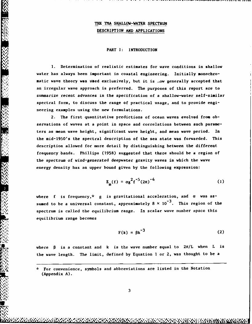
16. Bouws et al. (1985a) fitted the THA spectral form to over 2,800

wind sea spectra to test its viability and to determine if any parametric re-

lationships could be established linking the spectral parameters to the ex-

ternal wind field. In general the fit of the spectrum was of the same quality

as the fit of the JONSWAP spectrum to deepwater wind sea spectra. Examples of

the fit to field spectra are given in Figure 4.

THA parametric relationships

17. The relationships between the THA spectral parameters and various

dimensionless quantities such as dimensionless peak frequency and wave number

were examined by Bouws et al. (1985a). They determined that a and y could

be expressed by the following empirical expressions for all water depths:

a = 0.0078K 0 49 (22)

*y ¥ = 2.47K0 .3 9 (23)

10

100 610

80/10/25. 8.35

10 h m

1.0

0.1

0.01P0 0.10 0.20 0.30 0.40 0.50

100 -630

80/10125. 8.35h- 18m

10 -

1.0 -

0.1

0.010 0.10 0.20 0.30 0.40 0.50

100 710

80/10/25. 8.35h -25 m

10

1.0

0.1

!-I_

,a 0.010 0.10 0.20 0.30 0.40 0.50

.n,@I f,Hz

Figure 4. ThA spectra fit to field datafrom ARSLOE data set

.i

where

U2K = k (24)

g m

with

U = windspeed at 10 m elevation

g = acceleration of gravity

km = 2n/Lm = wave number for waves at peak frequency

L = wavelength associated with peak frequency f from linear wavem mtheory

Examination of the variation of o in the fitting of the spectra to the TMA

representation gave no statistical correlation, so it was suggested that the

mean values of

a = 0.07 f < f( m(0509 f > fm

are sufficient when using the TMA spectrum.

18. A certain amount of scatter was present in the plots from which the

parametric relationships were derived. Bouws et al. (1985b) demonstrated that

the scatter could be simulated by assuming that the error in determination of

windspeed was normally distributed with a standard deviation between 10 and

20 percent. They concluded that the methods used to determine windspeed could

easily contain errors on that order. The most remarkable consequences of the

TMA research were (a) showing that the effect of depth could be incorporated

solely through the dependence of K on depth, and (b) determining that there

was no apparent systematic dependence on bottom type.

19. The preceding equations provide a means of predicting the limiting

wind sea spectral shape in finite depth waters in terms of the windspeed and

the peak frequency. The procedure is to determine K from Equation 24, find

a and y (Equations 22 and 23, respectively), and then calculate ETA(f,h)

values using Equation 21. The 4b function is determined for each frequency

using either Equation 12 or (if a slightly less accurate answer can be toler-

ated) Equation 15. Significant wave height can be determined by numerically

integrating the resulting shallow-water spectrum and then applying the rela-

tionship for H given by Equation 19, but an easier approach is to usema

Vincent's depth-limited significant wave height expression given by

12

Equation 20, provided that wh < I for most of the energy containing

frequencies.

TMA internal parameterizations

20. Starting with Kitaigorodskii et al.'s (1975) basic equation for the

equilibrium range (Equation 2), Vincent (1985a) was able to derive an expres-

sion for a in terms of significant wave steepness e . This expression is

the following:

2 2a = 16n e (26)

where

& = significant wave steepness = E1/2/L (27)

E = total energy in the spectrum

L " = wavelength associated with f as defined in linear theory

This result is identical with that obtained by Huang et al. (1981) for a

JONSWAP spectrum in deep water. Field data support Vincent's formulation;

thus, Equation 26 holds for all water depths.

21. Equating Equation 26 and Equation 22 gives an expression for K in

terms of e which can then be put into Equation 23 to yield

y = 6614e 1.59 (28)

, ~ which should be valid for wind seas. The main advantage of this internal

parameterization is the ability to specify the equilibrium wind sea spectrum

associated with a given energy level.

22. It is an interesting exercise to show that Vincent's depth-limited

significant wave height equation (Equation 20) and the expression for a

(Equation 26) are the same. The energy E in Equation 27 can be given in

terms of H from the relationship of Equation 19. Substitution into Equa-mo

tion 26 yields

Hr 1/2 (29)mo nja Lm

40 and taking L = (gh)/ 2Tm in shallow water gives

H 0o (agh) 1/ 2 Tn (30)mo n m

13

The only difference between Equation 30 and Equation 20 is the 1.1 factor

which Vincent (1982) arrived at by assuming a cutoff frequency of 0.9 f ..Am

Equation 29 is a more general form of Equation 30, and it can be applied

throughout the shallow- and intermediate-water depth ranges when the appropri-

ate expression for L is used and a is found from Equation 22.~m23. To reiterate, significant wave heights H found using either

moEquation 29 or Equation 30 are the maximum values that can occur at that depth

for the given values of peak period and windspeed. In addition, Hmo calcu-lated for very shallow water can be substantially less than the significantd.

wave height If defined as the average of the highest 1/3 waves. H pro-s mo

vides an estimate of the energy contained in the wave spectrum, while H pro-5

vides a statistical estimation of the wave heights. This variation in shallow

water is due to the increasing nonlinearity in the waves. A full treatment of

this topic is provided in Thompson and Vincent (1985), and provision is made

for this effect in a later section of this report.24. Since Equation 29 reduces to Vincent's depth-limited result in

shallow water, it might be suspected that a similar exercise could be performed

for deep water. Replacing L in Equation 29 with the deepwater relationship,

L = (g/2n)T , replacing a with Equation 22, and nondimensionalizing re-mo m

sults in

/H 3o/2gmo = 0.0112 - (31)

when the exponent of K in Equation 22 is taken as 1/2. A similar result is

found if the deepwater fetch-limited equations for wave height and wave period

in the Shore Protection Manual (SPM) (1984) are combined, the only difference

being a coefficient of 0.0105 instead of 0.0112.

25. The expression for the fully developed wind sea significant wave

height in deep water can now be derived by replacing Tm in Equation 31 with

the fully developed wave period as defined in Equation 4. This results in

gHo=mo 0.238 (32)

U2

The only difference between Equation 32 and the expression for fully developed

deep water H given in the SPM (1984) is the value of 0.243 instead ofmo

0.238. This is remarkable because the SPM equation was arrived at by

14

consideration of the time necessary to reach full development of the JONSWAP

equations.

26. This exercise has illustrated that the internal and external

parameterizations for o can be applied for all water depths outside of the

surf zone. The ability to recover deepwater results is particularly interest-

ing since the parameterization of a as a function of f and windspeed wasm

done using data largely from shallow- and intermediate-water depths.

Wave Growth Limitation

Wave period limit

27. Vincent and Hughes (1985) examined the question of whether or not

finite depth wind waves reach a fully developed state where the peak spectral

frequency becomes fixed and no longer migrates toward lower frequencies,

regardless of the energy input. Evidence that such a cutoff frequency may

exist comes from the Lake Okeechobee and the Gulf of Mexico data used by

Bretschneider (1958) to develop shallow-water wave growth curves. Bret-2schneider plotted gT m/U versus gh/U and determined an empirical relation-

mmship for the cutoff frequency in shallow water. Vincent and Hughes pointed

out that the quenching of atmospheric input of energy, which occurs in deep

water when the celerity of the waves exceed the windspeed, did not appear to

occur in shallow water. This is because at a given depth all waves of fre-

quency less than f* have the same celerity, if f* is the highest frequency

where the shallow-water dispersion relation is a valid approximation. If the

deepwater growth mechanism is assumed, it would be possible to have windspeeds

in excess of the wave speed and still have wave growth.

28. Vincent and Hughes (1985) proposed that the cutoff frequency where

shallow-water wave growth would stop should be determined by a frequency where

the shallow-water dispersion relation held plus a further shift to slightly

lower frequencies due to resonant wave-wave interactions. This frequency is

defined as

whm= 2nf(- = 0.9 (33)

and it arises from Kitaigorodskii et al.'s (1975) observation that the tran-

-5 . . 3sition from a deepwater f equilibrium range to an f range for

15

S°"

shallow-water waves occurred when wh :- 1 The slight downward shift in

frequency is empirically represented by the 0.9 value.

29. Rearranging iquation 33, multiplying by g/U and noting Tm

1 1/fm , the following nondimensional expression results which may be compared

to Bretschneider's result:

,p..gT m =2 n(h12(4

U 0.9 U.2)

This comparison is made in Figure 5, and it demonstrates a reasonable fit to

the field data. The advantage of Equation 33 is that a value of windspeed is

not a factor in determining the fully developed cutoff frequency in shallow

water. In otoer words, it is assumed that once a fully developed condition

exists in shallow water, the peak frequency remains fixed regardless of any

increase in windspeed.

100

gT __ _ _ __ _ _ __ _ _ _

U .01

10 "|

10-3 102 101 100

gh

U 2

Figure 5. Relationship between dimensionless periodand depth (dashed line is Equation 34; solid line isBretschneider's (1958) empirical fit) (Vincent and

Hughes 1985)

Wave height limit

30. Bretschneider (1958) also presented nondimensional significant wave

height versus nondimensional depth for the shallow-water fully developed data.

Vincent and Hughes (1985) were able to show that Vincent's estimate for depth-

limited significant wave height (Equation 20) can be used to derive an expres-

sion for the fully developed case closely matching Bretschneider's empirical

formulation. They expressed k in Equation 24 asm

16

'V...

k 2 2t 27 0.9

m Lm (gh)1 /2T hm

where L is replaced by its shallow-water expression from linear theory and

T is found from Equation 33 for the fully developed case. Using this expres-msion for k , the value of af for the fully developed case is determined

from Equation 22 as

a = O.0074U/(gh) 1/2 (35)

where the 0.49 exponent of Equation 22 is taken as 1/2. Substituting Equa-

tion 35 for a and Equation 33 for T into Equation 20 yieldsU

H , 0.210U1/2 h

3 /4

-"HP = -(36)2 "1/4

g

where H is the significant wave height for the fully developed case. Non-

dimensionalizing by g/U 2 gives

gH 0.210 () (37)

U 0.210 )

Equation 37 is compared to Bretschneider's result in Figure 6.

31. The favorable fit of the equations for fully developed wave period

and wave height to the shallow-water field data of Bretschneider lend support

to the TMA shallow-water self-similar spectral form and to the parameteriza-

tions made for a . However, there are still many unanswered questions in-

volving the underlying physical processes which result in the TMA spectrum.

It must be noted that these shallow-water limitations are for full development

on a flat bottom, but they do provide a useful upper limit for some engineer-

ing purposes.

0

17

-I -"'.4....- : - - .X :: .- '.: > . :>, , , ,

gHs103

03 10-2 10 100

gh2

Figure 6. Relationship between dimensionless waveheight and depth (dashed line is Equation 37;solid line is Bretschneider's (1958) empirical fit

(Vincent and Hughes 1985)

18

%

.:-..-:*::tv c

PART III: SURF ZONE SPECTRA

32. In the formulation and parameterization of the TMA spectral form

by Bouws et al. (1985a) the data examined were restricted to those spectra re-

corded outside of the surf zone. They were uncertain of the appropriateness

of using linear wave theory in the surf zone to convert from wave number space

to frequency space via Kitaigorodskii et al.'s (1975) 0 function. Also,

outside the surf zone the balance of forces determining spectral evolution are

comprised of wind, breaking (largely at high frequencies), dissipation due to

a bottom boundary layer, and transfers of energy in the spectrum. Once the

surf zone is reached, major breaking occurs near the peak of the spectrum thus

introducing a separate concern. Vincent examined the fit of the TMA spectral

form to spectra collected well within the surf zone during the ARSLOE experi-

ment. (The surf zone spectra were not a part of the ARSLOE portion of the

data set used to determine the ThA parameters).*

Fit of TMA to Collected Spectra

. 33. The TMA form was fitted to the spectra only over the region up to

twice the spectral peak frequency 2f . Beyond this frequency forced har-m

monics begin to dominate the spectrum, while the TMA form is meant to represent

only free wave energy. Figure 7 is an example of the best fit obtained by

Vincent to a surf zone spectrum recorded in 1.7 m of water. A reasonable fit

is mace between the range of 0.5f to 2.Of , which is the principal energym m

containing region. At higher frequencies the TMA form underestimates the

energy content. Vincent (1985b) noted that the energy contained at these

higher frequencies increases as the depth decreases. This increased energy

represents the increasing nonlinearity of the long period wave components in

shallow water. Vincent suggested a modifying factor for the TMA spectral form,

but he lacked the necessary data to provide a generally applicable modification.

However, as a first approximation, the unmodified TMA spectrum can be used to

represent surf zone spectra if the spectral parameters can be estimated. Theresulting estimated significant wave height found using this approach was

within 10 percent of the actual values for the cases that Vincent examined.

Personal correspondence between Vincent and Hughes, January 1984.

19

" ,

.,V

.3 Cage 615 - 10/2S/80 - 0855 GIT

h- 1.7 m

a

0

i' -40

00.00 0.20 0.110 0.60 0.e0 1.o0,%,,.

f, Hz

Figure 7. Fit of TMA spectrum to surf zoneirregular wave spectrum

1.ote that the logarithmic scale for energy density used in Figure 7 makes it

appear that the difference in total energy between the TMA fit and the actual

spectrum is greater than it truly is.)

34. An unexpected result of this work was the reasonable fit of the

TMA spectral form to broad swell spectra in the surf zone obtained from both

the field and the laboratory. This is surprising for two reasons. First,

the broad swell is more indicative of a decaying than a growing sea state for

which the self-similar spectrum was proposed. Second, there is no reason to

expect that mechanically generated irregular waves in the laboratory should

follow the TMA form for wind waves since the primary forcing function (the

wind) is absent. This latter observation was found to be true for both char-

acteristic broad swell spectra outside the surf zone as well as for typical

wind sea spectra simulated in the laboratory. Figure 8 illustrates the fit-

ting of the TMA spectral form to laboratory data shoaled over a 1:30 slope.

Hypothesis for Energy Saturation

ZLocal saturation zone

35. Vincent (1985b), suggested a hypothesis for energy saturation of

irregular waves during shoaling by proposing a separation of the saturation

process during shoaling into two distinct types: the local and universal

20

L

-

--... ... .. " r ""w-.... - ' w' ' " * * '* I w• - r ."

-LANOSBOSV DATA

00 ,m

t.o

Ssea

sea

- 40 -5

'" zo. i

.099m .4;

0 O CO .SG AtO JE S34

Fro".acy. 0q

a. Spectrum typical of swell

50-LAORATORY DATA

O 00 TMA SP CTRUM FIT

40-

40 -0 to

30-

200

10-'492

0-0 A1) .40 A 86 IA

Frequency, hZ

b. Spectrum typical of wind seas

Figure 8. Fit of the TMA spectrum to laboratory data on1:30 slope (Vincent 1985b)

21F

saturation zones. As waves progress into finite depth waters, they first

enter a local saturation zone in the intermediate and shallow-water depths

where nonlinear wave-wave interactions shift energy away from the principal

energy containing frequencies to higher frequencies where it is dissipated by

deepwater breaking mechanisms. This is the region for which all the previous

TMA formulations and parameterizations for wind waves are valid. It appears

that broad swell spectra also can be fitted by the TMA form in this region,

but there is no external parameterization for a in this case.

Universal saturation zone

36. Eventually, if the water depth becomes sufficiently shallow, wave

breaking begins to occur at the peak of the spectrum, and dissipation dominates

the spectrum. Vincent (1985b) referred to this region as the universal satura-

tion zone. While there still may be some transfer of energy between frequen-

cies in this zone, the wave train is basically a series of nondispersive waves,

each breaking in sequence. The fact that the TMA spectral form could be fitted

to data gathered within the surf zone indicated to Vincent that the spectral

parameters could be obtained from the steepness equations (Equations 26 and 28)

if a saturated value for the energy could be obtained. Working on the hypothe-

sis that the largest wave at a given depth in the universal saturation zone is

controlled by the depth, Vincent (1985b) proposed

mo=Bh (38)

* where

h = water depth(39)

Rmax

BR Rso ms

and

R H /h for monochromatic wavesmax max

R =H/Hso 5 mo

where

H = average of the highest 1/3 wavesS

R = H /H 1.33ms max s

U

22

JO e•

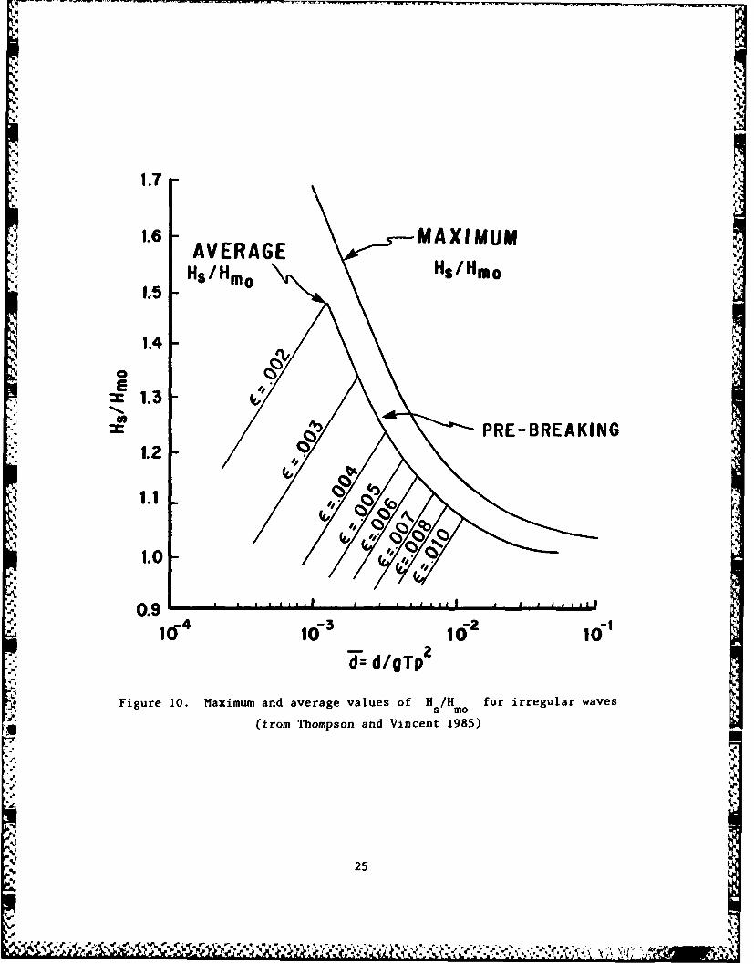
Values for Rmax can be obtained from Figure 9, which is reproduced from the

SPM (1984), and values for R can be found from the "average" line in Fig-

ure 10, which is reproduced from Thompson and Vincent (1985). For slopes

typical of most beaches, the coefficient B ranges between 0.55 and 0.65.

These values are consistent with the value of B = 0.6 suggested by Thornton

and Guza (1982), and unless the area of concern varies greatly from a "typical"

beach, the value of 0.6 for B is probably sufficient for engineering pur-

poses. The significant steepness is found from Equation 27 as

IH

(E1 2 -4 H Bh (40)I

Lm Lm 4(gh)1 2 Tm

when Equation 19 is used for H and the linear theory shallow-water wave-

length is substituted. The parameter o can now be found from Equation 26

hf2

of =- ( (41)

where

2nf(h\) (42)

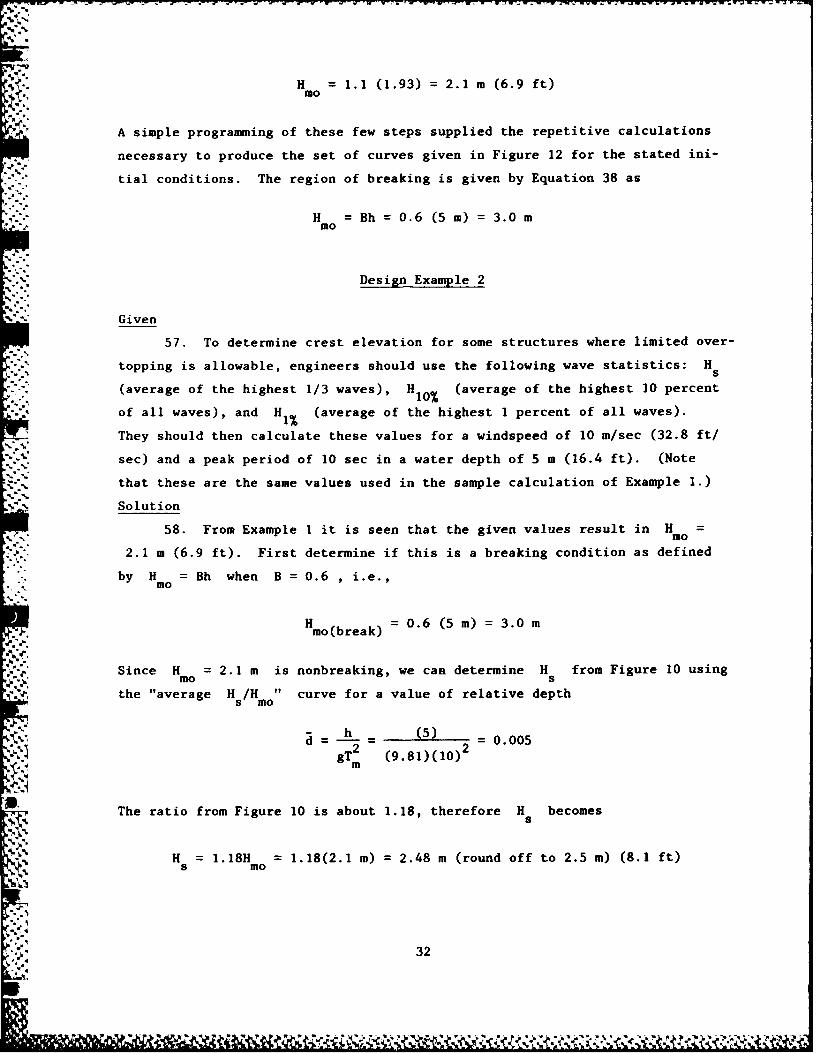
37. The ability of Equation 41 to'predict a in very shallow water .

shown in Figure 11 (from Vincent 1984). The figure shows reasonable agree-

ment for both laboratory and field data in the universal saturation zone.

Note that in the universal saturation zone H varies linearly with depthmo

(Equation 38), while in the local saturation zone Ho varies with the square

root of the depth (Equation 20). Also note that the equation for H in thema

local saturation zone (Equation 20) reduces to the expression for Hmo in the

universal saturation zone (Equation 38) when Equation 41 is substituted for

a This is not surprising since both equations are linked to the equation for

a in terms of e.

38. It is somewhat difficult to define a demarcation line between the

local saturation zone and the universal saturation zone. Ideally there should

be some limiting value of significant steepness beyond which wave breaking at

the spectral peak is assured.

23

'VH~4~.~~~ K~~ti4~li~c l

4 4

T r

-44-

II00

ti $

4-9.

--T

00

- - 0

24

.1.

-11

1.7

:.6 AVERAGE" Hs/Hm Hs/HM° i

1.4

.-' =' / RE- BREAKI NG

'.'-1.4

o m

PRE-BREKIN

1.25

0.9•( 1-3 1-2 1-1

Figured= d/gTp2

Fiue10. Mlaximum and average values of Hs/Ho for irregular waves

-u" (from Thompson and Vincent 1985)

..

,

'A.

",4: ,. " J "

' , r q . . • , -D- "." - - . % - ,. - .... '

II0.03 0ARSLOE F IE LD DATA

UHIGH STEEPNESS, LAB.£LOW STEEPNESS, LAB.

0.02U

w

CL

0.01 m

o I ° I

0 0.01 0.02 0.03

ALPHA OBSERVED

Figure 11. Alpha predicted versus alpha observed (from Vincent 1984)

w..2

-'..-.. 0.02 --

PART IV: DISCUSSION

39. Thus far the focus of this report has been on past developments in

the specification of self-similar spectral forms and their role in the develop-

ment of the new THA spectral form. By adding more and more terms to Phillips'

(1958) representation of the limiting energy density in the equilibrium range,

researchers progressively specified a self-similar spectral shape for deep

water (Pierson-Moskowitz), a fetch-limited deepwater spectrum (JONSWAP), a

shallow-water equilibrium range (Kitaigorodskii et al.), and finally a self-

similar equilibrium spectral form valid at all water depths (THA).

40. The self-similar parametric THA representation was shown to have

the ability to represent wind waves and broad swell, and it appears that both

the deepwater and shallow-water limits merge with previously obtained empirical

results. It was seen also that the THA form even fit very shallow surf zone

spectra up to twice the peak frequency.

Physical Implications of the THA Spectral Form

41. The fact that the self-similar TMA form can describe wind sea spec-

tra in deep, intermediate, or shallow water reinforces the conclusion of

Kitaigorodskii et al. (1975) that the basic scaling lies in k-space rather

than in frequency space. Also, the linear theory dispersion relation seems

adequate for converting from wave number space to frequency space via the 0

factor.

42. Both the JONSWAP and the THA spectral forms extended the k-3 scal-

ing for the equilibrium range across the entire spectrum. There is no physical

explanation as to why this scaling should be valid, but years of experience

using the JONSWAP form, coupled with the relative good fit of the TMA form to

shallow-water spectra, indicates that the scaling does hold outside the equi-

librium range.

43. Self-similarity in spectral form implies that there is a relative

balance between the wind energy input, energy transfers within the spectrum,

and energy dissipation. This balance is maintained and limited to produce a

consistent spectral shape. No analyses have been made into the very difficult

problem of the spectral balance between the various source/sink terms such as

nonlinear wave-wave interactions, wave dissipation, atmospheric input, bottom

27

%.'

friction, percolation, etc., for the TMA data set. However, it is tentativelyconcluded that the bottom friction effect in the dissipation of wave energy is

substantially less than originally thought. This conclusion is based on the

observation that the parametric relationships provide equally good spectral

approximations over a wide variety of depths and bottom materials. Thus it is

unlikely that bottom dissipation would be a dominant influence on spectral

shape. With the establishment of the TMA shape, study into the various source/

sink terms now can be restricted to combinations which will produce a self-

similar shape. Bottom friction for typical beaches is thought to be more im-

portant for swell than for wind seas.

44. Kitaigorodskii et al.'s (1975) equilibrium range was intended for

the case of a horizontal bottom, but the parameterization and applicition of

the TMA spectrum to data from gently sloping bottoms up to slopes of 1:100

indicate that the self-similar equilibrium form evolves rapidly enough to ade-

quately describe the spectral transformation over gentle slopes. Steep sloped

beaches might not permit the equilibrium condition to be reached; hence, the

TMA spectrum could well represent an unattainable limit on a steep slope.

45. Vincent (1985b) sums up the TMA spectral form as "...a quantitative

description of the wave transformation process with a useful parameterization

scheme." He adds that while many of the principal physical processes occurring

in wave shoaling have been identified, a deterministic description is still in

the future.

Assumptions and Limitations of the TMA Spectral Form

46. The primary underlying assumption invoked when applying the TMA

spectrum and the prognostic equations is that the wind sea is at a steady

state or equilibrium condition. This means that the wind has been steady long

enough (as yet undefined) for the waves to reach equilibrium and that the

bottom topography is a gentle slope with smoothly varying features and without

complexities which might cause rapid alteration of the wave train. Until

*. further data are examined, a slope steepness guideline of 1:100 is suggested

which arises from the limit of the TMA data set. While steeper slopes might

be able to maintain the TMA equilibrium condition, the worst that can happen

by using the THA approximation on a steep slope is a conservative estimate of

the maximum possible significant wave height for the given conditions. Note

28

-jb

that laboratory data on a 1:30 slope were adequately described using the TMA

representation.

47. The ThA spectrum as it is presently parameterized cannot be used

in fetch- or duration-limited shallow-water wave growth situations since it

is a final steady state form. Fetch- or duration-limited design in shallow

water needs to be conducted using numerical models (for complex regions) or

wave forecasting curves such as provided in ETL 1110-2-305 (Vincent and Lock-

hart 1984). Future developments will probably provide a THA fetch- and

duration-limited form paralleling the deepwater JONSWAP equations.

48. The THA spectral form is for a single-peaked spectrum containing

only minor low-frequency energy. In most instances large wave conditions will

result from either a local storm or swell resulting from a nearby storm. These

spectra will probably propagate toward shore as a single-peaked spectrum de-

-" scribable by the THA shape. The THA formulation does not handle multipeaked

spectra which, according to Thompson (1980), constitute over 60 percent of the

coastal wave conditions in the United States. However, most of the multi-

peaked cases are of low energy and of minor importance for engineering design.

The TMA shape may be used to describe the individual spectral peaks.

49. The shallow-water limits to wave growth derived as a cutoff fre-

quency and a limiting significant wave height fit the field data and provide

useful engineering guidance. The limits are strictly for full development

over a horizontal bottom or a gently sloping bottom.

50. The TMA prognostic equations require specifications of either

(a) U , h , and fm 1 or (b) =f(H , h , and f) Vincent (1984)

'" ~suggests that when wave conditions are steady and the combination of beach

slope and propagation distance are sufficiently small, then f may be pro-

jected from deep water into shallow water. In other words, the peak frequency

doesn't shift during shoaling. Field data from two 1980 storms at Duck, North

Carolina, indicated that f did not change more than 10 percent over a 36 kmm

distance in which the depth changed from 36 to 2 m. In cases where wind

- fields and bottom conditions are highly inhomogeneous and fm is expected to

shift, a fully time-dependent spectral model is needed to determine f inm

shallow water.

1'

29

2

PART V: ENGINEERING APPLICATIONS

51. The preceding formulations for a self-similar equilibrium spectrum

for all water depths can provide useful engineering design guidance because

the equilibrium spectrum puts constraints on the expected energy levels and

spectral shapes under given conditions. While it is impossible to list every

conceivable application of the THA spectrum, the following short examples il-

lustrate several engineering uses.

Numerical Models

52. Some of the current shallow-water wave growth and propagation

numerical models can simulate wave propagation over complex bathymetry during

unsteady wind conditions. These models typically contain many source/sink

terms, some of which can be quite site specific. In some applications it is

possible for the models to give exaggerated results because there is no effec-

tive upper limit to the wave growth. This can be corrected by constraining

the numerical simulation to an upper limit of growth on the high frequency

side of the spectral peak as defined by the ThA spectrum.

53. Oceanographers at CERC illustrated the usefulness of the TMA spec-

tral form as an upper limit when they modified an existing numerical wave

growth spectral model and ran several simulations, with and without the TMA

prescribed limit. Generally, it was found that this particular numerical

model yielded unrealistically high results for high windspeeds and for beach

slopes of 1:200. In other words, sufficient energy dissipation through bottom

friction and other sink terms did not occur. When the slope was very mild

(1:2,000), bottom friction attenuated the waves adequately. Incorporating the

TMA limiting spectral form into the numerical model has made it a better en-

gineering tool; however, this does not relieve the engineer from responsible

calibration and verification of the model.

Design Example 1

Given

54. For a smoothly varying bottom slope, construct a set of design

curves showing the depth-limited significant wave height H as a function

30

%

.-.

of peak spectral period T and windspeed U. The given water depth is 5 mm

(16 ft).

Solution

55. It is first necessary to choose the proper equation for H,0

(either Equation 29 or 30). This is done by determining the wave frequency

where Wh=,i.e.,

w= 2nf'(h/g) 1/2 = 1

or

.1/2

P (9.81/5)1 12/2n = 0.22 Hz

which is T' 4.5 sec. When the principal energy containing frequencies

have periods greater than 4.5 sec, Equation 30 can be used. We will assume

that f'= 1.5 f mor T m= 1.5 T' = 6.75 sec. Any calculations made form m

peak periods less than 6.75 sec should be done using Equation 29 with Lm

being determined using the intermediate depth linear dispersion relation.

The calculations are done as follows:

For U = 10 m/sec (32.8 ft/sec) and T = 10 sec, first find

L = (gh) /2T = [(9.81)(5)] 1 2 10 = 70 m (230 ft)S,-m m

Next find K from Equation 24.

U22n (10) 2(2n)K -- =0- .915°gL m (9.81)(70)

OC 56. Using Equation 22,

0.49 0.49fa = 0.0078 K = 0.0078 (0.915) = 0.00747

and the H associated with this T and U is by Equation 30mo m

To-Hmo = 1 (agh)1/2Tm = [(0.00747)(9.81)(5)]1/2 (10) = 1.93 m (6.3 ft)

To be slightly conservative (10 percent), use the 1.1 factor as given in

Vincent's original derivation (Equation 20) to finally arrive at

31

H = 1.1 (1.93) = 2.1 m (6.9 ft)mo

A simple programming of these few steps supplied the repetitive calculations

necessary to produce the set of curves given in Figure 12 for the stated ini-

tial conditions. The region of breaking is given by Equation 38 as

H = Bh = 0.6 (5 m) = 3.0 mmo

Design Example 2

Given

57. To determine crest elevation for some structures where limited over-

topping is allowable, engineers should use the following wave statistics: H s

(average of the highest 1/3 waves), H (average of the highest 10 percent10%

of all waves), and H (average of the highest 1 percent of all waves).

They should then calculate these values for a windspeed of 10 m/sec (32.8 ft/

sec) and a peak period of 10 sec in a water depth of 5 m (16.4 ft). (Note

that these are the same values used in the sample calculation of Example 1.)

Solution

58. From Example 1 it is seen that the given values result in H =( " mo

2.1 m (6.9 ft). First determine if this is a breaking condition as defined

by H = Bh when B = 0.6 , i.e.,mo

H = 0.6 (5 m) = 3.0 mii . mo (break)

Since H = 2.1 m is nonbreaking, we can determine H from Figure 10 usingmo5the "average H s/H MO" curve for a value of relative depth

= h 2 (5) = 0.005

gT (9.81)(10)2

The ratio from Figure 10 is about 1.18, therefore H becomes

H = 1.18H = 1.18(2.1 m) 2.48 m (round off to 2.5 m) (8.1 ft)s mo

32

44~

0

CI D 0 ,

'A E4C4.) 7a

CDC

0 U0

'4 01z 0Vb f -"'' '

C!33

The values for H and H are now found using the expressions given in10% 1%

the SPM (1984).

H = 1.27 H = 1.27(2.48) = 3.15 m (round off to 3.2 m) (10.3 ft)10% s

H = 1.67 H = 1.67(2.48) = 4.14 m (round off to 4.2 m) (13.6 ft)

Note that the above calculations imply that the Rayleigh distribution of wave

heights is valid under the given conditions, while the highest possible wave

at this depth by monochromatic theory is about 0.76 (5 m) = 3.8 m. Thus the

"* tail of the wave height distribution will be truncated by breaking.

Design Example 3

Given

59. Determine the conditions under which a project built in 7 m (23 ft)

of water would be subjected to breaking wave conditions (i.e., surf zone con-

ditions) caused by irregular waves with a peak period of 11 sec.

Solution

60. The H for the breaking limit (universal saturation) is found• .'w'.mo

from Equation 38 as

H = Bh = 0.6 (7 m) = 4.2 m (13.8 ft)mo

The spectral parameter a can be found from Equation 41 with w determined

from Equation 42, i.e.,='' gl2 _ (;811/2

w. ;Uhm 2nf =1/ 2n 7

m 11 =9 ---. /2 0.4825(BWh)12) 2_ 2

.o = h 2= [0.6)(0.4825)/22 = 0.021

61. Next, use Equation 22 to find what value of K will produce the

following value of or at the given depth and peak period:

"0.4o = 0.0078K 0 4 9

34

or

K = (a/0.0078) 1 / 0 . 4 9 = (0.021/0.0078)1/0.49 = 7.55

From Equation 24 with

2'"" _ 2 _ 2n 2k 2 2 2n 0.0689 rad/m

m (gh)l/2 Tm 9"81)(7)] 1/ 2 ( 1 1 )

we get

U = (Kg/k m )1/2 = [(7.55)(9.81)/0.689]=1/2 32.8 r/sec (107.6

This windspeed is the sustained wind necessary to develop the equilibrium

* - breaking condition at the site for the given peak period. It corresponds

to speeds on the order of 73 mph which is a full hurricane force wind.

Design Example 4

Given

62. A wind sea has a significant wave height H of 2 m and a peakmo

spectral period T of 8 sec in a water depth of 10 m. Determine the corre-m

sponding H in 4-m water depth, assuming no refraction or diffraction and)"-""mo

that the peak period remains constant.

Solution

63. From Equation 29,

H1 () /2 L, and H = 0 2

Let

in 10 m in 4 m

H1 =H H =Hmo 2 mo

L, L L =L1 m 2 m

Taking the ratio of these two relationsnips yields

.~ '.?35

-1 1- ,a-~

1H(H )/ (L)

64. The ratio al/a 2 can be. found using Equation 22 as

11L2/2i2 i2, I L

Substituting this relationship into the previous equation gives

H 3/4

which is good under the restrictive assumptions of no refraction and diffrac-_ * tion and that the wind is equal and constant at both sites.

65. Using linear wave theory to find the wavelength associated with the

peak spectral period (assumed to remain constant at 8 sec):

L1 = 70.9 m at h = 10 m

-. L2 = 48.0 m at h = 4 m

Thus

H 1 _709\/4

- = (09 1.342/

so that-- . H

H2 . 3 23 1.5 m H at a water depth h= 4 m1.34 1.34 mo

If the significant wave height had been shoaled using linear wave theory,

H1 /H2 would have been 0.7 and H at h = 4 m would have been 2.9 m.

36

AA

. .

PART VI: SUMMARY

4.-M

66. Recent work by Bouws et al. has led to a self-similar equilibrium

spectral form for all water depths. This form, called the THA spectrum, arises

from the substitution of Kitaigorodskii et al.'s finite depth equilibrium range

for the deepwater equilibrium range in the JONSWAP energy density equation.

Examination of over 2,800 field spectra in varying water depths and under di-

verse conditions resulted in a parameterization for the spectral variables in

terms of depth, peak frequency, and windspeed. The parameters a and y

were also expressed in terms of significant wave steepness. A simple expres-

sion for the energy-based significant wave height Hmo was derived from the

TMA spectral form making it possible to predict the depth-limited equilibrium

H in either intermediate or shallow water.mo

67. The TMA spectral representation recovers the deepwater fully devel-

oped results when the deepwater limits are applied, and it follows the fully

developed shallow-water empirical results when the suggested cutoff frequency

relationship for shallow water is applied.

68. Within the surf zone the TMA spectrum can be fit rather well up to

twice the peak frequency. Beyond that point highly nonlinear processes cause

a deviation from the TMA form. A distinction was made between local and uni-

versal saturation, and a method of estimating the spectral parameters within

the surf zone was presented.

69. The success of the TMA spectrum as a simple spectral model rein-

forces Kitaigorodskii et al.'s (1975) conclusion that the basic self-similarity

scaling is in k-space. Many of the principal physical processes which bring

about the TMA form have been identified but not quantified. Applications and

examples were presented to illustrate some uses of the TMA results under the

stated assumptions and limitations.

, .3

.0.-,[

"-.X

.dg',37

REFERENCES

Bouws, E., et al. 1985a. "Similarity of the Wind Wave Spectrum in FiniteDepth Water, Part I - Spectral Form," Journal of Geophysical Research, Vol 90,No. Cl, pp 975-986.

Bouws, E., et al. 1985b (in review). "Similarity of the Wind Wave Spectrum inFinite Depth Water, Part II - Quasi-Equilibrium Relations," Journal of Geophy-sical Research.

Bretschneider, C. L. 1958. "Revisions in Wave Forecasting: Deep and ShallowWater," Proceedings of the 6th Conference on Coastal Engineering, AmericanSociety of Civil Engineers, pp 30-67.

Gadzhiyev, Y. Z., and Kratsitsky, B. B. 1978. "The Equilibrium Range ofthe Frequency Spectra of Wind-Generated Waves in a Sea of Finite Depth,"Izrestiya, Atmospheric and Ocean Physics, USSR, Vol 14, No. 3, pp 238-242.

Hasselmann, K., et al. 1973. "Measurements of Wind Wave Growth and SwellDecay During the Joint Sea Wave Project (JONSWAP)," Report No. 12, DeuthshesHydrographisches Institut, Hamburg.Huang, N. E., et al. 1981. "A Unified Two-Parameter Wave Spectral Model for

a General Sea State," Journal of Fluid Mechanics, Vol 112, pp 203-224.

Kitaigorodskii, S. A., Krasitskii, V. P., and Zaslavskii, M. M. 1975. "On

Phillip's Theory of Equilibrium Range in the Spectra of Wind-Generated GravityWaves," Journal of Physical Oceanography, Vol 5, pp 410-420.

Kruseman, P. 1976. "Two Practical Methods of Forecasting Wave Componentswith Periods Between 10 and 25 Seconds Near Hoek van Holland," WetenschapelijkRapport 76-1, Koninklijk Nederlands Meteorologisch Instituut, The Netherlands.

Louguet-Higgins, M. S. 1952. "On the Statistical Distribution of the Heightsof Sea Waves," Journal of Marine Research, Vol XI, No. 3, pp 245-266.

Mitsuyasu, H. 1981. "Directional Spectra of Ocean Waves in Generation Area,"Proceedings of the Conference on Directional Wave Spectra Applications, Ameri-can Society of Civil Engineers, pp 87-101.Phillips, 0. M. 1958. "The Equilibrium Range in the Spectrum of Wind-

Generated Ocean Waves," Journal of Fluid Mechanics, Vol 4, pp 426-434.

Pierson, W. J. and Moskowitz, L. 1964. "A Proposed Spectral Form for FullyDeveloped Windseas Based on the Similarity Theory of S. A. Kitaigorodskii,"Journal of Geophysical Research, Vol 69, pp 5181-5190.

Shore Protection Manual. 1984. 4th ed., 2 vols, US Army Engineer WaterwaysExperiment Station, Coastal Engineering Research Center, US Government Print-ing Office, Washington, DC.

Thompson, E. F. 1980. "Energy Spectra in Shallow US Coastal Waters," Tech-nical Paper 80-2, US Army Engineer Waterways Experiment Station, Coastal Engi-neering Research Center, Vicksburg, Miss.

*Thompson, E. F. and Vincent, C. L. 1983. "Prediction of Wave Height inShallow Water," Proceedings of Coastal Structures '83, American Society ofCivil Engineers, pp 1000-1008.

38

* Thompson, E. F. and Vincent, C. L. 1985. "Significant Wave Height forShallow Water Design," Journal of the Waterway, Port, Coastal, and OceanDivision, American Society of Civil Engineers, Vol III, No. 5.

Thornton, E. B. and Guza, R. T. 1982. "Energy Saturation and Phase SpeedsMeasured on a Natural Beach," Journal of Geophysical Research, Vol 87, No. C12,pp 9499-9508.

Toba, Y. 1973. "Local Balance in the Air-Sea Boundary Processes: III - Onthe Spectrum of Wind Waves," Journal of the Oceanographic Society of Japan,Vol 29, pp 209-220.

Vincent, C. L. 1982. "Depth-Limited Significant Wave Height: A SpectralApproach," Technical Report 82-3, US Army Engineer Waterways Experiment Sta-tion, Coastal Engineering Research Center, Vicksburg, Miss.

• 1984. "Shoaling and Transmission of Wind Seas," 3rd Conferenceon Meteorology of the Coastal Zone, American Meteorological Society, pp 41-43,

_iami,_ Fa 1985a. "Equilibrium Range Coefficient of Wind Wave Spectra inWater of Finite Depth," submitted to Journal of Geophysical Research.

1985b (accepted for publication). "Energy Saturation ofIrregular Waves During Shoaling," American Society of Civil Engineers.

Vincent, C. L., and Hughes, S. A. 1985. "A Note on Wind Wave Growth in Shal-low Water," Journal of Waterway, Port, Coastal and Ocean Division, AmericanSociety of Civil Engineers, Vol III, No. 4.

Vincent, C. L. and Lockhart, J. H. 1984. "Determining Sheltered Water WaveCharacteristics," ETL 1110-2-305, Headquarters, Department of the Army, OfficeChief of Engineers, Washington, DC.

39

1l

V

*i- .~

a, a

APPENDIX A: NOTATION

-p

k'A

I"a.

a..

a.m.a.'

-A-.

Al

.5 -

-Js *-' --

B Parameter

d Relative depth

E Total spectral energy

E (f) Energy density for JONSWAP spectrum

E (f) Equilibrium energy density in frequency spacem

E (f,h) Finite depth equilibrium energy density in frequency space

E pm(f) Energy density for Pierson-Moskowitz spectrum

E TMA(f,h) Energy density for TMA spectrumf Frequency

f' Frequency

F* Highest freqeuncy where shallow-water dispersion relation holds

f Cut off frequency* c

F(k) Equilibrium energy density in wave number space

f Spectral peak frequencym

9 Gravitational constant

h Water depth

H H for fully developed wind sea over a flat bottomI: mo

H Maximum monochromatic wave heightmaxH Zero-moment wave heightmo

H Average height of the 1/3 highest wavesH

H1% Average of highest 1 percent of waves

10% Average of highest 10 percent of waves

k Wave number

k Wave number for waves at peak frequencym

L Wavelength

L Wavelength associated with frequency f by linear wave theorym U

L moDeepwater equivalent of Lmo m

R Relative maximum wave height for monochromatic wavesmaxR Ratio of H to Hms max sR Ratio of H to Hso s mo

Tv Period

T Spectral peak periodm

U 10-m-high windspeed

X Fetch distance

aSpectral parameter

A constant

A2

~ >*.OA

V Spectral parameter

e Significant wave steepness

K Dimensionless wave number

S3.14...

o Spectral parameter

o a Spectral parametera

a b Spectral parameter

*(2wf,h) Finite depth factor

Circular frequency

4h Depth dependent frequency

W hm '"h evaluated at fM

_4 mm

A33