ERSA 39th EUROPEAN CONGRESS 1999

THE TITTLE OF THE PAPER: ANALYSIS OF THE CONCENTRATION OF THE

STRUCTURAL FUNDS IN THE AUTONOMOUS COMMUNITIES IN SPAIN

THE AUTHORS NAMES: J. BARÓ LLINÀS, M.A. CABASÉS PIQUÉ, M.J. GÓMEZ

THE AFFILIATION OF THE AUTHORS: Professors Applied Economics Department

THE ADDRESS OF EACH AUTHOR

Dr. JOAN BARÓ LLINÀSDepartamento de Economía AplicadaFacultad de Derecho y EconomiaPlaza Victor Siurana, 1 25003 LLEIDATf. 973 70 20 31

Dra. Mª ANGELS CABASES PIQUEDepartamento de Economia AplicadaFacultad de Derecho y EconomiaPlaza Victor Siurana, 1 25003 LLEIDATf. 973 70 20 31

Mª JESÚS GÓMEZ ADILLÓNDepartamento de Economia AplicadaFacultad de Derecho y EconomiaPlaza Victor Siurana, 1 25003 LLEIDAM.Jesus.Gomez@econap.UdL.esTf. 973 70 20 31Fax 973 70 21 15

THE THEME TO WICH PAPER RELATES: THEORY AND METHODOLOGY OF

REGIONAL SCIENCE

ANALYSIS OF THE CONCENTRATION OF STRUCTURAL FUNDS

IN THE AUTONOMOUS COMMUNITIES IN SPAIN

ABSTRACT

In this paper we analyse the distribution in Spain, of the European Regional

Development Fund community structural help, considering its importance in volume. This

survey is carried out in each autonomous community and in two five-year periods, being the

first period 1989-1992 and the second one 1994-1999.

First of all we work out measures of concentration in order to point out the

difference in the concentration of the ERDF per capita, assigned by the European Union to

the Autonomous Communities in the two periods which are analysed.

The indicators propose are measures derive from the concentration graph, so that we

can observe the existence of greater or minor concentration depending on the degree of

convexity of the graph line, and obtaining distances of interest between the straight line of

equidistribution and the graph line which reflect the inequality in the distribution of the

ERDF per capita.

Secondly, a typological analysis of the Autonomous Communities is carried out, for

the two periods, taking into account the economic variables which affect the distribution of

the European Regional Fund and with the purpose of describing repercussions of the

implementation of the MAC.

INTRODUCTION

Since its incorporation into the EEC in 1986, Spain has benefited from European

Community Structural Fund aid. The Treaty of Rome, which constituted the EEC and was

signed in 1958, referred directly to the reduction of inequalities between the member states,

but only did so in a general way. During 1958 the ESF (European Social Fund) was created

and in 1962 the EAGGF- Guidance Section (European Agricultural Guidance and

Guarantee Fund) was created, and these intervened in European community regional policy,

in a modest and implicit way. It was not until seventeen years later, in 1975 that with the

creation of the ERDF (European Regional Development Fund) a boost was given to the

Community's regional policies.

The incorporation of the Spain and Portugal (1986), considerably increased the

discrepancies in income between the different regions of the European Community. Shortly

after this the Treaty underwent a major modification with the adoption of the Single

European Act (1987). The principle of Cohesion was established, reflected in Article 130 of

the new Treaty, which reinforces the European Community regional policy and its

instruments of implementation.

Article 130 announced the reform of the Structural Funds (ERDF, ESF and EAGGF-G)

which implied a new design of these funds and the doubling of their economic value.

The objectives of this reform of the structural funds are identified with problems, which in a

general way affect an entire region or administrative territory within the European Union.

The areas eligible for structural funds are indicated, with five different objectives:

Objective 1: To promote the development and adaptation of less advanced regions.

Objective 2: To reconvert those regions gravely affected by the industrial crisis.

Objective 3: To fight against long-term unemployment.

Objective 4: To facilitate professional occupation of young people.

Objective 5: Contains two objectives:

Objective 5a: To adapt the structures of production, transformation and

commercialisation in agriculture and forestry.

Objective 5b: To promote the development of rural areas.

In 1989, a new stage began, as the reform of the structural funds entered into force and the

European Community regional policy now had at its disposal instruments to redress

imbalances between the different regions of the European Union. The same year saw the

birth of the CSFs (Community Support Frameworks) applying to periods of several years,

and these were to designed coordinate actions and available resources. In 1993 the CSF for

1989-1993 ended and the 1994-1999 was negotiated.

In Spain, out of the total volume of aid proceeding from structural funds, the ERDF (with

Objectives 1, 2 and 5b) contributes more than 50% of the total aid. If we study the aid by

objectives, it is concentrated in areas eligible for Objective 1, an important part of the funds

being received for this objective (aid for less advanced regions).

This study analyses the distribution, in Spain, of the community structural aid from the

ERDF, given its importance in terms of volume, by autonomous region and during two five

year periods, the first running from 1989 and 1993, and the second period between 1994 and

1999.

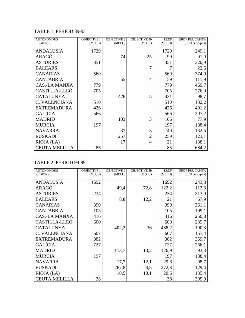
TABLE 1: PERIOD 89-93

AUTONOMOUSREGIONS

OBJECTIVE 1(MECU)

OBJECTIVE 2(MECU)

OBJECTIVE 5b(MECU)

ERDF(MECU)

ERDF PER CAPITA(ECU per capita)

ANDALUSIAARAGÓASTURIESBALEARSCANÀRIASCANTABRIACAS.-LA MANXACASTILLA-LLEÓCATALUNYAC. VALENCIANAEXTREMADURAGALÍCIAMADRIDMURCIANAVARRAEUSKADIRIOJA (LA)CEUTA MELILLA

1729

351

560

779705

510426566

197

85

74

55

426

103

3725717

25

7

4

5

3

324

172999

3517

56059

77970543151042656610619740

2592185

249,191,0

320,922,6

374,9111,9469,7276,998,7

132,2401,2207,277,9

188,4132,5123,1138,1684,2

TABLE 2. PERIOD 94-99

AUTONOMOUSREGIONS

OBJECTIVE 1(MECU)

OBJECTIVE 2(MECU)

OBJECTIVE 5b(MECU)

ERDF(MECU)

ERDF PER CAPITA(ECU per capita)

ANDALUSIAARAGÓASTURIESBALEARSCANÀRIASCANTABRIACAS.-LA MANXACASTILLA-LLEÓCATALUNYAC. VALENCIANAEXTREMADURAGALÍCIAMADRIDMURCIANAVARRAEUSKADIRIOJA (LA)CEUTA MELILLA

1692

234

390105416600

607382727

197

38

49,4

8,8

402,2

113,7

17,7267,810,5

72,8

12,2

36

13,2

12,14,5

10,1

1692122,2

23421

390105416600

438,2607382727

126,9197

29,8272,320,6

38

243,8112,3213,967,9

261,1199,1250,8235,7100,3157,4359,7266,193,3

188,498,7

129,4135,4305,9

Specifically, measures of concentration are calculated with the sole objective of underlining

the differences in ERDF concentration per capita, assigned by the European Union to the

Autonomous Regions during the two periods under study. A purely quantitative calculation

is performed of the differences, without entering into the analysis of the volume of projects

financed in the different Autonomous Regions.

The indicators presented are measures derived from the concentration curve, since the

Lorenz Diagram, with an initial graphic approach, allows us to visualise the existence of

greater or lesser concentration according to the degree of convexity of the curve.

From this representation distances of interest arise between the straight line of equal

distribution and the curve which reflect the inequality in the distribution of the ERDF funds

per capita, always taking into account only the population assigned for objectives 1, 2 and

5b. The surface area separating the straight line from the curve is a good measure of

concentration of the variable.

Taking into account the empirical observation of the data and the economic nature of the

ERDF variable per capita, different theoretical functions of concentration are estimated:

- Kakwani-Podder model (1973): q(p) = pα · e-β(1-p) with α ≥ 1 β >0

- Kakwani model (1980): q(p) = p - A· pα · (1-p)β with A, α and β >0

- Gupta model (1984): q(p) = p · Ap-1 with A >1

The three equations possess the usual properties of a concentration curve:

- Range between 0 and 1: p ∈ (0,1) → q(p) ∈ (0,1)

- Increasing monotony: q'(p) ≥ 0

- Convexity: q''(p) ≥ 0

In addition these are equations which are highly operative for the calculation of the different

indicators of concentration.

In the context of this study, identification in terms of random variable is applied to

p as the fraction of population up to a level x, and

q(p) as the fraction of ERDF funds accumulated up to level x

distributions being ordered in terms of per capita.

The models are estimated using the squared minimums after conversion method:

- Ln q(p) = α ln + β (p-1) + ε

- Ln (p-q(p)) = ln A + α ln p + β ln (1-p) + ε

- Ln q(p) -ln p = ln A * (p-1) + ε

These models have been chosen, firstly because they were created as concentration curves

that allow the calculation of measures of inequality in the distribution of funds, and secondly

because they are models which can be suitably adapted to the data presented.

CONCENTRATION MEASURES USED

From the estimations concentration measures have been calculated which are obtained from

the curves and which allow the quantitative calculation of the differences in, and

concentration of, the ERDF funds per capita during the two periods under consideration. So

they show a greater concentration when the value that they take is greater and therefore the

greater the inequality existing in the distribution of the ERDF funds per capita.

1.- g Index.

Gini's coefficient of concentration, which is well known, and corresponds to double the area

enclosed between the two lines of distribution, that is, double the average of all the distances

between population and ERDF accumulation, as shown by graph 1.

g = 2E(p-q(p)) = 1 - 2E (q(p))

The expression of the index in the models considered takes on the following form:

Calculation of the Gini (g) index.

Kakwani-Podder1 – 2e-

β ∑∞

= ++β

0i

i

!i)i1a(

Kakwani 2A B( α+1, β+1); with B(α+1, β+1) Beta Euler

Gupta

AlnA

2A2AlnA2AlnA2

2 −+−

2. - P Index

The P for Pietra coefficient is associated to the greater distance existing between the

population and ERDF accumulations, a distance which is observed in the ERDF volume

expected:

P= pµ - q(pµ)

It is known that the concentration curve has a unitary gradient at the point ((pì , q (pì )), the

moment in which the distances between the two lines is at its maximum (Graph 2).

max [Fξ(x)-qξ(x)] = pµ - q (pµ) → q'(p) = 1

The coefficient P is normally used as the lowest level in the Gini index, at the same time that

it responds to the double of the area of the greatest triangle that can be inscribed within the

figure, i.e., that it coincides with half of the average relative difference and which in any case

fulfils that P = DMR ≤ g

2

3.- d* Index

Picks up the lack of phasing between the accumulated population and ERDF both in the

mean (Ml) and in the median (ME). On the one hand, p(Ml)-0.5 measures the inequality

between two groups with equal ERDF and on the other, 0.5-q(p(ME)) measures the

inequality of the two groups with equal population, both correspond with the distances

which separate the line of equal distribution and the concentration curve from the

geometrical centre of the graph (Graph 3), its simple aggregation leads us to the index:

d* = p(Ml) - q(p(Me))

Its usage is not widely extended and it is rarely used in theoretical studies on concentration.

4.- d' Index

In the same way that we have considered central distances in the curve, it makes sense to

measure the inequality gap that exists in the first quartile (0.25-q(p(Q1)) and in the third

quartile (0.75-q(p(Q3)) (Graph 4.) The sum of these two distances gives sense to the d'

coefficient:

d'=1 - [q(p(Q1)) + q(p(Q3))]

This is not a very widely used indicator either, its advantage lies in the fact that it admits the

generalisation of any of the other quartiles, and in addition its calculation is immediate in any

concentration function.

Graph 1: g Index Graph 2: P Index

F

q

01

1

F

q

01

1

F(m)

q(m)

Graph 3: d* Index Graph 4: d’ Index

0,5

0,5

F

q

F(Ml)

q(Me)

01

1

0,75F

q

01

1

0,25

q(Q1)

q(Q3)

CONCENTRATION MODEL ESTIMATES

The three models offer adaptations of quality and an elevated degree of adherence for the

two periods considered. Below we present the results of the estimates of the three models in

tables 1, 2 and 3.

Table 1: Results of the Kakwani-Podder model estimation

Predictor Coef DesvEst razón-t1989-1993 Ln p 1,32011 0,04609 28,64

p-1 0,5071 0,1273 3,98

s = 0,1280 F = 3.110,36

1994-1999 Ln p 1,07240 0,01389 77,22p-1 0,68232 0,03832 17,81

s = 0,03935 F = 27.035,42

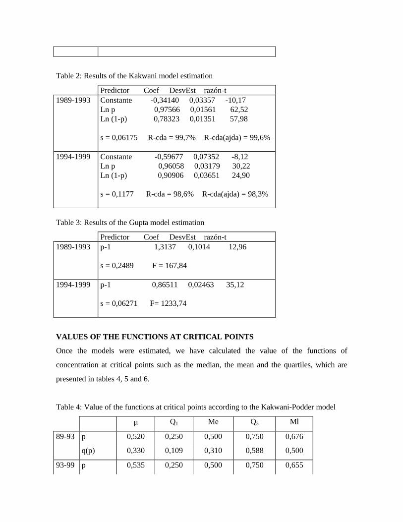
Table 2: Results of the Kakwani model estimation

Predictor Coef DesvEst razón-t1989-1993 Constante -0,34140 0,03357 -10,17

Ln p 0,97566 0,01561 62,52Ln (1-p) 0,78323 0,01351 57,98

s = 0,06175 R-cda = 99,7% R-cda(ajda) = 99,6%

1994-1999 Constante -0,59677 0,07352 -8,12Ln p 0,96058 0,03179 30,22Ln (1-p) 0,90906 0,03651 24,90

s = 0,1177 R-cda = 98,6% R-cda(ajda) = 98,3%

Table 3: Results of the Gupta model estimation

Predictor Coef DesvEst razón-t1989-1993 p-1 1,3137 0,1014 12,96

s = 0,2489 F = 167,84

1994-1999 p-1 0,86511 0,02463 35,12

s = 0,06271 F= 1233,74

VALUES OF THE FUNCTIONS AT CRITICAL POINTS

Once the models were estimated, we have calculated the value of the functions of

concentration at critical points such as the median, the mean and the quartiles, which are

presented in tables 4, 5 and 6.

Table 4: Value of the functions at critical points according to the Kakwani-Podder model

µ Q1 Me Q3 Ml

89-93 p 0,520 0,250 0,500 0,750 0,676

q(p) 0,330 0,109 0,310 0,588 0,500

93-99 p 0,535 0,250 0,500 0,750 0,655

q(p) 0,372 0,135 0,338 0,619 0,500

Table 5: Value of the functions at critical points according to the Kakwani model

µ Q1 Me Q3 Ml

89-93 p 0,555 0,250 0,500 0,750 0,697

q(p) 0,342 0,103 0,289 0,568 0,500

93-99 p 0,513 0,250 0,500 0,750 0,645

q(p) 0,363 0,138 0,349 0,631 0,500

Table 6: Value of the functions at critical points according to the Gupta model

µ Q1 Me Q3 Ml

89-93 p 0,570 0,250 0,500 0,750 0,725

q(p) 0,324 0,093 0,259 0,540 0,500

93-99 p 0,550 0,250 0,500 0,750 0,667

q(p) 0,372 0,130 0,324 0,604 0,500

The values obtained in the three functions of concentration for the critical points considered

are very close, and therefore they lead us to very similar conclusions.

Thus for example, if we consider the critical point of the median of the distribution, as a

value which differentiates the total of communities in two groups (in the first group the

volume of funds does not reach half of the total and in the second it exceeds half), practically

50% of the communities have received a volume of funds above the total median in the

second period. Continuing with this line, and taking the median as the dividing point of the

groups, we can establish relationships between the volume of ERDF funds in each group and

the volume of funds of all the communities. The values obtained for the three functions are

presented in tables 7, 8 and 9.

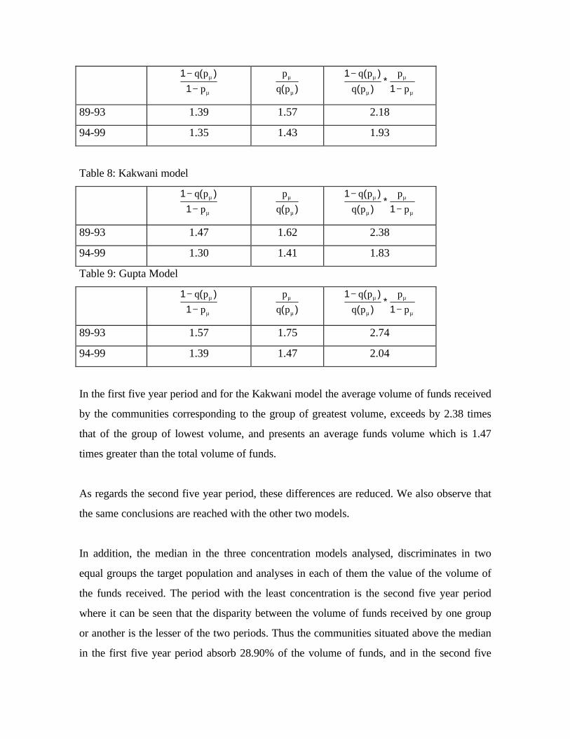
Table 7: Kakwani-Podder model

µ

µ

−

−

p

pq

1

)(1

)( µ

µ

pq

p

µ

µ

µ

µ

−

−

p

p

pq

pq

1*

)(

)(1

89-93 1.39 1.57 2.18

94-99 1.35 1.43 1.93

Table 8: Kakwani model

µ

µ

−

−

p

pq

1

)(1

)( µ

µ

pq

p

µ

µ

µ

µ

−

−

p

p

pq

pq

1*

)(

)(1

89-93 1.47 1.62 2.38

94-99 1.30 1.41 1.83

Table 9: Gupta Model

µ

µ

−

−

p

pq

1

)(1

)( µ

µ

pq

p

µ

µ

µ

µ

−

−

p

p

pq

pq

1*

)(

)(1

89-93 1.57 1.75 2.74

94-99 1.39 1.47 2.04

In the first five year period and for the Kakwani model the average volume of funds received

by the communities corresponding to the group of greatest volume, exceeds by 2.38 times

that of the group of lowest volume, and presents an average funds volume which is 1.47

times greater than the total volume of funds.

As regards the second five year period, these differences are reduced. We also observe that

the same conclusions are reached with the other two models.

In addition, the median in the three concentration models analysed, discriminates in two

equal groups the target population and analyses in each of them the value of the volume of

the funds received. The period with the least concentration is the second five year period

where it can be seen that the disparity between the volume of funds received by one group

or another is the lesser of the two periods. Thus the communities situated above the median

in the first five year period absorb 28.90% of the volume of funds, and in the second five

year period, they absorb 34.93%. The same conclusion is reached through any of the three

models analysed.

MEASURES OF CONCENTRATION

To follow we present the calculation of the different measures of concentration for the three

models considered.

Table 10. Concentration measures for the Kakwani-Podder model.

P d* d' g89-93 0,189 0,365 0,301 0,260

94-99 0,162 0,316 0,245 0,216

Table 11. Concentration measures for the Kakwani model

P d* d' g89-93 0,213 0,407 0,327 0,291

94-99 0,150 0,295 0,230 0,205

Table 12. Concentration measures for the Gupta model

P d* d' g89-93 0,246 0,472 0,366 0,324

94-99 0,177 0,342 0,265 0,235

It is possible to observe how the indices derived from the three curves indicate that the

tendency of the concentration is lesser in the second period from 94-99 than in the first

period 89-93. Taking into account that in the two five year periods and in the three

functions, the values are low, i.e., the inequality is not very great. The second period

presents lesser inequality in the distribution of the ERDF funds among the populations

eligible for the objectives.

CONCLUSIONS

In the concentration curves representation for the two periods under study, and for the three

models considered, according to figures 1, 2 and 3, we can see how the ERDF funds

concentration per capita has decreased in the second five year period with respect to the

first, as the measures previously described indicate. Thus, the curve for the 94-99 period is

much closer to the imaginary line of equal distribution, and therefore less inequality exists in

the distribution of the funds. We can conclude that with the application of the Community

Support Framework for this second five year period, the difference existing in the

assignation of funds to the Autonomous Regions of the State of Spain has reduced with

respect to the previous period.

This study corroborates the conclusions of the European Commission with representation in

Barcelona, according to which the reduction of ERDF per capita in the second five year

period is palpable in the Spanish Autonomous Regions, in which it has been managed to

reduce the inequality of the distribution of the ERDF funds per capita amongst the eligible

populations.

FIGURE 1: KAKWANI-PODDER MODEL CONCENTRATION CURVES

1,00,50,0

1,0

0,5

0,0

p

q(p)

- - - - 94-99

------ 89-93

FIGURE 2. KAKWANI MODEL CONCENTRATION CURVES

1,00,50,0

1,0

0,5

0,0

p

q(p) - - - - 94-99

------ 89-93

FIGURE 3. GUPTA MODEL CONCENTRATION CURVES

0,0 0,5 1,0

0,0

0,5

1,0

p

q(p)

- - - - 94-99

------ 89-93

I. Estimation of the concentration curves Kawanni-Podder model:q(p) 89-93 = p1,3201 · e-0,5071(1-p)

q(p) 94-99 = p1,0724 · e-0,6832(1-p)

p q(p) 89-93 q(p) 94-99 p q(p) 89-93 q(p) 94-99

2 0,01 0,00139 3 0,02 0,00348 4 0,03 0,00597 5 0,04 0,00877 6 0,05 0,01184 7 0,06 0,01514 8 0,07 0,01865 9 0,08 0,02235 10 0,09 0,02625 11 0,10 0,03032 12 0,11 0,03456 13 0,12 0,03896 14 0,13 0,04352 15 0,14 0,04824 16 0,15 0,05311 17 0,16 0,05812 18 0,17 0,06329 19 0,18 0,06859 20 0,19 0,07404 21 0,20 0,07963 22 0,21 0,08536 23 0,22 0,09123 24 0,23 0,09724 25 0,24 0,10338 26 0,25 0,10966 27 0,26 0,11607 28 0,27 0,12262 29 0,28 0,12931 30 0,29 0,13613 31 0,30 0,14308 32 0,31 0,15017 33 0,32 0,15739 34 0,33 0,16475 35 0,34 0,17225 36 0,35 0,17987 37 0,36 0,18764 38 0,37 0,19554 39 0,38 0,20358 40 0,39 0,21175 41 0,40 0,22006 42 0,41 0,22851 43 0,42 0,23709 44 0,43 0,24581 45 0,44 0,25468 46 0,45 0,26368 47 0,46 0,27282 48 0,47 0,28211 49 0,48 0,29153 50 0,49 0,30110 51 0,50 0,31081

0,00365 0,00772 0,01201 0,01646 0,02105 0,02577 0,03061 0,03557 0,04063 0,04580 0,05108 0,05646 0,06194 0,06753 0,07321 0,07899 0,08488 0,09086 0,09694 0,10312 0,10941 0,11579 0,12228 0,12886 0,13555 0,14234 0,14924 0,15623 0,16334 0,17054 0,17786 0,18528 0,19280 0,20044 0,20818 0,21604 0,22400 0,23208 0,24027 0,24857 0,25699 0,26552 0,27417 0,28294 0,29183 0,30083 0,30996 0,31921 0,32858 0,33807

52 0,51 0,32066 53 0,52 0,33066 54 0,53 0,34080 55 0,54 0,35109 56 0,55 0,36153 57 0,56 0,37212 58 0,57 0,38285 59 0,58 0,39373 60 0,59 0,40477 61 0,60 0,41595 62 0,61 0,42729 63 0,62 0,43878 64 0,63 0,45042 65 0,64 0,46222 66 0,65 0,47418 67 0,66 0,48629 68 0,67 0,49857 69 0,68 0,51100 70 0,69 0,52359 71 0,70 0,53634 72 0,71 0,54926 73 0,72 0,56234 74 0,73 0,57558 75 0,74 0,58899 76 0,75 0,60257 77 0,76 0,61632 78 0,77 0,63023 79 0,78 0,64432 80 0,79 0,65858 81 0,80 0,67301 82 0,81 0,68762 83 0,82 0,70240 84 0,83 0,71736 85 0,84 0,73249 86 0,85 0,74781 87 0,86 0,76331 88 0,87 0,77898 89 0,88 0,79485 90 0,89 0,81089 91 0,90 0,82713 92 0,91 0,84355 93 0,92 0,86016 94 0,93 0,87696 95 0,94 0,89395 96 0,95 0,91113 97 0,96 0,92851 98 0,97 0,94609 99 0,98 0,96386 100 0,99 0,98183 101 1,00 1,00000

0,34769 0,35744 0,36732 0,37732 0,38745 0,39772 0,40811 0,41864 0,42931 0,44011 0,45105 0,46212 0,47334 0,48470 0,49620 0,50784 0,51963 0,53157 0,54365 0,55588 0,56827 0,58081 0,59350 0,60634 0,61935 0,63251 0,64583 0,65931 0,67296 0,68677 0,70074 0,71488 0,72919 0,74368 0,75833 0,77316 0,78817 0,80335 0,81871 0,83425 0,84998 0,86588 0,88198 0,89826 0,91473 0,93140 0,94825 0,96530 0,98255 1,00000

II. Estimation of the concentration curves Kawanni model:q(p) 89-93 = p – 0,710774 · p0,97566 ·(1-p)0,78323

q(p) 94-99 = p – 0,550587 · p0,96058 ·(1-p)0,90906

p q(p) 89-93 q(p) 94-99 p q(p) 89-93 q(p) 94-99

2 0,01 0,00211 3 0,02 0,00461 4 0,03 0,00732 5 0,04 0,01022 6 0,05 0,01328 7 0,06 0,01649 8 0,07 0,01985 9 0,08 0,02336 10 0,09 0,02700 11 0,10 0,03078 12 0,11 0,03470 13 0,12 0,03875 14 0,13 0,04293 15 0,14 0,04724 16 0,15 0,05169 17 0,16 0,05627 18 0,17 0,06097 19 0,18 0,06581 20 0,19 0,07078 21 0,20 0,07587 22 0,21 0,08110 23 0,22 0,08645 24 0,23 0,09193 25 0,24 0,09754 26 0,25 0,10329 27 0,26 0,10916 28 0,27 0,11516 29 0,28 0,12129 30 0,29 0,12755 31 0,30 0,13394 32 0,31 0,14047 33 0,32 0,14712 34 0,33 0,15391 35 0,34 0,16083 36 0,35 0,16788 37 0,36 0,17506 38 0,37 0,18238 39 0,38 0,18983 40 0,39 0,19742 41 0,40 0,20514 42 0,41 0,21300 43 0,42 0,22100 44 0,43 0,22913 45 0,44 0,23740 46 0,45 0,24581 47 0,46 0,25436 48 0,47 0,26305 49 0,48 0,27189 50 0,49 0,28086 51 0,50 0,28998

0,00346 0,00739 0,01155 0,01591 0,02043 0,02511 0,02993 0,03489 0,03999 0,04522 0,05057 0,05605 0,06165 0,06738 0,07322 0,07919 0,08527 0,09147 0,09778 0,10421 0,11076 0,11742 0,12419 0,13108 0,13808 0,14519 0,15241 0,15975 0,16720 0,17476 0,18243 0,19022 0,19811 0,20612 0,21423 0,22246 0,23080 0,23925 0,24781 0,25648 0,26527 0,27416 0,28317 0,29229 0,30151 0,31086 0,32031 0,32987 0,33955 0,34934

52 0,51 0,29925 53 0,52 0,30866 54 0,53 0,31821 55 0,54 0,32792 56 0,55 0,33777 57 0,56 0,34778 58 0,57 0,35793 59 0,58 0,36824 60 0,59 0,37871 61 0,60 0,38933 62 0,61 0,40011 63 0,62 0,41105 64 0,63 0,42215 65 0,64 0,43341 66 0,65 0,44484 67 0,66 0,45643 68 0,67 0,46820 69 0,68 0,48014 70 0,69 0,49225 71 0,70 0,50454 72 0,71 0,51701 73 0,72 0,52966 74 0,73 0,54250 75 0,74 0,55553 76 0,75 0,56875 77 0,76 0,58217 78 0,77 0,59579 79 0,78 0,60962 80 0,79 0,62366 81 0,80 0,63792 82 0,81 0,65240 83 0,82 0,66712 84 0,83 0,68207 85 0,84 0,69728 86 0,85 0,71274 87 0,86 0,72846 88 0,87 0,74447 89 0,88 0,76078 90 0,89 0,77740 91 0,90 0,79435 92 0,91 0,81167 93 0,92 0,82937 94 0,93 0,84750 95 0,94 0,86612 96 0,95 0,88529 97 0,96 0,90511 98 0,97 0,92573 99 0,98 0,94745 100 0,99 0,97090 101 1,00 1,00000

0,35924 0,36925 0,37938 0,38962 0,39997 0,41044 0,42102 0,43172 0,44253 0,45345 0,46450 0,47566 0,48693 0,49832 0,50983 0,52146 0,53321 0,54508 0,55706 0,56917 0,58140 0,59375 0,60623 0,61883 0,63156 0,64441 0,65739 0,67050 0,68375 0,69712 0,71063 0,72427 0,73806 0,75198 0,76605 0,78026 0,79462 0,80914 0,82381 0,83865 0,85366 0,86885 0,88422 0,89980 0,91559 0,93162 0,94793 0,96459 0,98171 1,00000

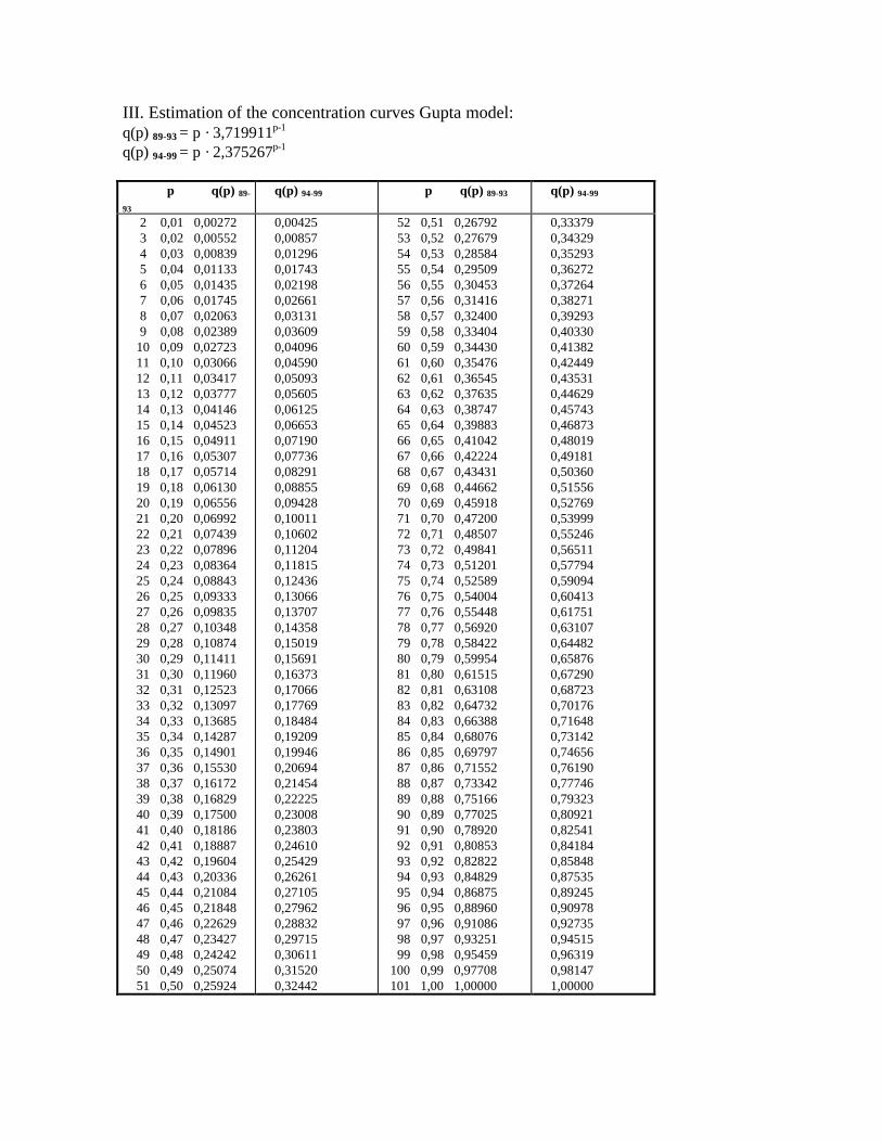
III. Estimation of the concentration curves Gupta model:q(p) 89-93 = p · 3,719911p-1

q(p) 94-99 = p · 2,375267p-1

p q(p) 89-

93

q(p) 94-99 p q(p) 89-93 q(p) 94-99

2 0,01 0,00272 3 0,02 0,00552 4 0,03 0,00839 5 0,04 0,01133 6 0,05 0,01435 7 0,06 0,01745 8 0,07 0,02063 9 0,08 0,02389 10 0,09 0,02723 11 0,10 0,03066 12 0,11 0,03417 13 0,12 0,03777 14 0,13 0,04146 15 0,14 0,04523 16 0,15 0,04911 17 0,16 0,05307 18 0,17 0,05714 19 0,18 0,06130 20 0,19 0,06556 21 0,20 0,06992 22 0,21 0,07439 23 0,22 0,07896 24 0,23 0,08364 25 0,24 0,08843 26 0,25 0,09333 27 0,26 0,09835 28 0,27 0,10348 29 0,28 0,10874 30 0,29 0,11411 31 0,30 0,11960 32 0,31 0,12523 33 0,32 0,13097 34 0,33 0,13685 35 0,34 0,14287 36 0,35 0,14901 37 0,36 0,15530 38 0,37 0,16172 39 0,38 0,16829 40 0,39 0,17500 41 0,40 0,18186 42 0,41 0,18887 43 0,42 0,19604 44 0,43 0,20336 45 0,44 0,21084 46 0,45 0,21848 47 0,46 0,22629 48 0,47 0,23427 49 0,48 0,24242 50 0,49 0,25074 51 0,50 0,25924

0,00425 0,00857 0,01296 0,01743 0,02198 0,02661 0,03131 0,03609 0,04096 0,04590 0,05093 0,05605 0,06125 0,06653 0,07190 0,07736 0,08291 0,08855 0,09428 0,10011 0,10602 0,11204 0,11815 0,12436 0,13066 0,13707 0,14358 0,15019 0,15691 0,16373 0,17066 0,17769 0,18484 0,19209 0,19946 0,20694 0,21454 0,22225 0,23008 0,23803 0,24610 0,25429 0,26261 0,27105 0,27962 0,28832 0,29715 0,30611 0,31520 0,32442

52 0,51 0,26792 53 0,52 0,27679 54 0,53 0,28584 55 0,54 0,29509 56 0,55 0,30453 57 0,56 0,31416 58 0,57 0,32400 59 0,58 0,33404 60 0,59 0,34430 61 0,60 0,35476 62 0,61 0,36545 63 0,62 0,37635 64 0,63 0,38747 65 0,64 0,39883 66 0,65 0,41042 67 0,66 0,42224 68 0,67 0,43431 69 0,68 0,44662 70 0,69 0,45918 71 0,70 0,47200 72 0,71 0,48507 73 0,72 0,49841 74 0,73 0,51201 75 0,74 0,52589 76 0,75 0,54004 77 0,76 0,55448 78 0,77 0,56920 79 0,78 0,58422 80 0,79 0,59954 81 0,80 0,61515 82 0,81 0,63108 83 0,82 0,64732 84 0,83 0,66388 85 0,84 0,68076 86 0,85 0,69797 87 0,86 0,71552 88 0,87 0,73342 89 0,88 0,75166 90 0,89 0,77025 91 0,90 0,78920 92 0,91 0,80853 93 0,92 0,82822 94 0,93 0,84829 95 0,94 0,86875 96 0,95 0,88960 97 0,96 0,91086 98 0,97 0,93251 99 0,98 0,95459 100 0,99 0,97708 101 1,00 1,00000

0,33379 0,34329 0,35293 0,36272 0,37264 0,38271 0,39293 0,40330 0,41382 0,42449 0,43531 0,44629 0,45743 0,46873 0,48019 0,49181 0,50360 0,51556 0,52769 0,53999 0,55246 0,56511 0,57794 0,59094 0,60413 0,61751 0,63107 0,64482 0,65876 0,67290 0,68723 0,70176 0,71648 0,73142 0,74656 0,76190 0,77746 0,79323 0,80921 0,82541 0,84184 0,85848 0,87535 0,89245 0,90978 0,92735 0,94515 0,96319 0,98147 1,00000

REFERENCES

ANUARIO ECONÓMICO COMARCAL, 1994. Institut d'Estadística de Catalunya.Generalitat de Catalunya, pp. 30-82.

ANUARIO ESTADÍSTICO DE CATALUNYA,1997. Institut d'Estadística de Catalunya.Generalitat de Catalunya, pp. 147-155.

BARÓ, J.,1988. Función e índice de concentración de algunas distribuciones truncadas.Comunicación II reunión ASEPELT-España. Valladolid.

BARÓ, J. ,1991. Aplicaciones del modelo de kakwani al análisis de la distribución de larenta. Document de Treball núm. 9101. Institut d'Estudis Laborals. Universtitat deBarcelona.

BARÓ, J. and MORATAL,V.,1984.Concentración y distribuciones truncadas. Qüestió,Vol.8 núm.3 pp. 127-132

BARÓ, J. and TORRELLES, E.,1989. Sobre las medidas de concentración. Document deTreball 8904. Institut d'Estudis Laborals. Universitat de Barcelona.

BARÓ, J.,1989. Descomposició del índice de Gini. Comunicación en III ReuniónASEPELT-España. Sevilla

CABASÉS PIQUÉ, M.A. (1993). "Models i índex de concentració. Aplicació al volumempresarial de Lleida". Tesis Doctoral.

COMISIÓN EUROPEA (1995). "Los Fondos Estructurales en 1994". Sexto informe anual.

GASTWIRTH, J.L.,1972. Estimation of the Lorenz Curve and Gini Index. Review ofEconomics and Statistics, Vol.LIV nú.3 pp. 306-316

GIORGI, G. and PALLINI,A. ,1986. Di talune soglie inferior e superiore del rapporto diconcentrazione". Metron, Vol XLIV, núm. 1-4

GUPTA, M.R. ,1984. Notes and comments. Functional Form for Estimation the LorenzCurve. Econometrica , 52, pp. 1313-1314.

KAKWANI, N.C. and PODDER, N., 1973.On the Estimation of Lorenz Curves fromGrouped observations. International Economic Review,14 pp. 278-292.

KAKWANI,N.C., 1980 a. On a class of Poverty Measures. Econometrica núm. 48.

KAKWANI, N.C.,1980 b. Income inequality and poverty. Oxford University Press.

PATRONAT CATALÀ PRO EUROPA (1997). " Els fons estructurals a Catalunya”.

Aplicació i perspectives de la política estrctural i de cohesió de la Unió Europea.