The Time Variation in Risk Appetite and Uncertainty

Geert Bekaert Eric C. Engstrom Nancy R. Xu∗

November 10, 2017

*PRELIMINARY*

Abstract

We develop new measures of time-varying risk aversion and economic uncertainty that

can be calculated from observable financial information at high frequencies. Our approach

has four important elements. First, we formulate a dynamic no-arbitrage asset pricing model

that consistently prices all assets under assumptions regarding the joint dynamics among

asset-specific cash flow dynamics, macroeconomic fundamentals and risk aversion. Second,

both the fundamentals and cash flow dynamics feature time-varying heteroskedasticity and

non-Gaussianity to accommodate dynamics observed in the data, which we document. This

allows us to distinguish time variation in economic uncertainty (the amount of risk) from

time variation in risk aversion (the price of risk). Third, despite featuring non-Gaussian

dynamics, the model retains closed-form solutions for asset prices. Fourth, our approach

exploits information on realized volatility and option prices for the two main risky asset

classes, equities and corporate bonds, to help identify and differentiate economic uncertainty

from risk aversion. We find that equity variance risk premiums are very informative about

risk aversion, whereas credit spreads and corporate bond volatility are highly correlated

with economic uncertainty. Model-implied risk premiums beat standard instrument sets

predicting excess returns on equity and corporate bonds. A financial proxy to our economic

uncertainty predicts output growth negatively and significantly, even in the presence of the

VIX.

∗Bekaert is with Columbia University and the NBER, Engstrom is with the Federal Reserve Board of Gover-

nors, Xu is with Columbia University. The views expressed in this document do not necessarily reflect those of

the Federal Reserve System, its Board of Governors, or staff. All errors are the sole responsibility of the authors.

Contact: Xu (nancy.xu@gsb.columbia.edu)

1 Introduction

It has become increasingly commonplace to assume that changes in risk appetites are an

important determinant of asset price dynamics. For instance, the behavioral finance literature

(see, e.g., Lemmon and Portnaiguina (2006) and Baker and Wurgler (2006) for a discussion)

has developed “sentiment indices,” and there are now a wide variety of “risk aversion” or

“sentiment” indicators available, created by financial institutions (see Coudert and Gex (2008)

for a survey). The “structural” dynamic asset pricing literature has meanwhile proposed time-

varying risk aversion as a potential explanation for salient asset price features (see Campbell

and Cochrane (1999) and a large number of related articles), whereas reduced-form asset pricing

models, aiming to simultaneously explaining stock return dynamics and option prices, have also

concluded that time-varying prices of risk are important drivers of stock return and option price

dynamics (see Bakshi and Wu, 2010; Bollerslev, Gibson, and Zhou, 2011; Broadie, Chernov,

and Johannes, 2007). Risk aversion has also featured prominently in recent monetary economics

papers that suggest a potential link between loose monetary policy and the risk appetite of

market participants, spurring a literature on what structural economic factors would drive risk

aversion changes (see, e.g., Rajan, 2006; Adrian and Shin, 2009; Bekaert, Hoerova, and Lo Duca,

2013). In international finance, Miranda-Agrippino and Rey (2015) and Rey (2015) suggest that

global risk aversion is a key transmission mechanism for US monetary policy to be exported to

countries worldwide and is a major source of asset return comovements across countries (see

also Xu, 2017). Finally, several papers on sovereign bonds (e.g. Bernoth and Erdogan, 2012)

have stressed the importance of global risk aversion in explaining their dynamics and contagion

across countries.

Our goal is to develop a measure of time-varying risk aversion that is relatively easy

to estimate and compute, so that it can be compared to other indices and tracked over time.

However, the measure should also correct for deficiencies plaguing many of the current measures.

First, it must control for macro-economic uncertainty; we want to separately identify both the

aversion to risk (the price of risk) and the amount of risk. To do so, we build on dynamic

asset pricing theory. Essentially, our risk aversion measure constitutes a second factor in the

pricing kernel that is not driven by macroeconomic fundamentals. The modeling framework

therefore is related, but not identical, to the habit models of Campbell and Cochrane (1999),

Menzly, Santos and Veronesi (2004) and Wachter (2006). As in Bekaert, Engstrom and Xing

(2009) and Bekaert, Engstrom and Grenadier (2010), we allow for a stochastic risk aversion

component that is not perfectly correlated with fundamentals. As an important byproduct,

we also derive a measure of economic uncertainty, which constitutes an alternative to recent

measures (e.g. Juardo, Ludvigson, and Ng, 2015). In the model, asset prices are linked to cash

flow dynamics and preferences in an internally consistent fashion. In contrast, a number of

articles develop time-varying risk aversion measures motivated by models that really assume

“constant” prices of risk and hence are inherently inconsistent (see, for example, Bollerslev,

Gibson, and Zhou, 2011), or fail to fully model the link between fundamentals and asset prices

(see e.g. Bekaert and Hoerova, 2016). Third, as is well-known, asset prices and returns display

1

dynamics with highly non-Gaussian distributions that are time varying. In fact, a number of

articles (see Bollerslev and Todorov, 2011; Liu, Pan, and Wang, 2004; Santa-Clara and Yan,

2010) suggest that compensation for rare events (“jumps”) accounts for a large fraction of

equity risk premiums. To accommodate these non-linearities in a tractable fashion, we use

the Bad Environment-Good Environment (BEGE, henceforth) framework developed in Bekaert

and Engstrom (2017). Shocks are modeled as the sum of two variables with de-meaned gamma

distributions, whose shape parameters vary through time. The model delivers conditional non-

Gaussian shocks, with changes in “good” or “bad” volatility also changing the conditional

distribution of the process. Finally, our data include macroeconomic fundamentals, asset prices,

and options prices. The dynamic asset pricing and options literatures indirectly reveal the

difficulty in interpreting many existing risk aversion indicators. Often they use information

such as the VIX or return risk premiums that are obviously driven by both the amount of risk

and risk aversion. Disentangling the two is not straightforward. Articles such as Drechsler and

Yaron (2008), Bollerslev et al. (2009) and Bekaert and Hoerova (2016) point towards the use

of the VIX in combination with the (conditional) expected variance as particularly informative

about risk preferences. Therefore, this paper is also related to the literature on extracting

information about risk and risk preferences from option prices (for a survey, see Gai and Vause,

2006).

The use of different asset classes in deriving a single measure of risk aversion imposes the

important assumption that different markets are priced in an integrated setting. This may not

(always) be the case. During the 2007-2009 global crisis, it was widely recognized that arbitrage

opportunities surfaced between asset classes and sometimes within an asset class (for instance,

between Treasury bonds of different maturities, see e.g. Hu, Pan, and Wang, 2013). There may

well be a link between risk aversion and the existence of arbitrage opportunities. That is, in

uncertain, risk averse times, there is insufficient risky capital available, which causes different

asset classes to be priced incorrectly (see, for example, Gilchrist, Yankov, and Zakrajsek, 2009).

While consistent pricing across risky asset classes is a maintained assumption in our benchmark

model, we can easily test for consistent pricing by examining risk aversion measures implied by

different asset classes. We provide an example by comparing risk aversions filtered from risky

assets only and from both risky assets and Treasury bonds.

The remainder of the paper is organized as follows. Sections 2 and 3 presents the model

and estimation strategy in detail. Section 4 briefly outlines the data we use. Section 5 extracts

risk aversion and uncertainty from asset prices and discusses the links between the risk aversion

estimates and various financial variables. We also examine the behavior of the indices around

the Bear Stearns and Lehman Brothers bankruptcies. In Section 6, we link our measures of

risk appetite and uncertainty to alternative indices including ones produced by practitioners.

In Section 7, we discuss the case of risk aversion involving Treasury bonds. Concluding remarks

are in Section 8.

2

2 Modeling Risk Appetite and Uncertainty

In this section, we first define our concept of risk aversion in general terms in Section 2.1.

We then build a dynamic model with stochastic risk aversion and macro-economic factors af-

fecting the cash flows processes of two main risky asset classes, corporate bonds and equity.

The state variables are described in Section 2.2 and the pricing kernel in Section 2.3.

2.1 General Strategy

An ideal measure of risk aversion would be model free and not confound time variation

in economic uncertainty with time variation in risk aversion. There are many attempts in the

literature to approximate this ideal, but invariably various modeling and statistical assumptions

are necessary to tie down risk aversion. For example, in the options literature, a number

of articles (Aıt-Sahalia and Lo, 2000; Engle and Rosenberg, 2002; Jackwerth, 2000; Bakshi,

Kapadia and Madan, 2003; Britten-Jones and Neuberger, 2000) appear at first glance to infer

risk aversion from equity options prices in a general fashion, but it is generally the case that the

utility function is assumed to be of a particular form and/or to depend only on stock prices.

Another strand of the literature relies on general properties of pricing kernels. Using a

strictly positive pricing kernel or stochastic discount factor, Mt+1, no-arbitrage conditions imply

that for all gross returns, R,

Et [Mt+1Rt+1] = 1 (1)

It is then straightforward to derive that any asset’s expected excess return can be written as

an asset specific risk exposure (“beta”, or βt) times a price of risk (or λt), which applies to all

assets (see also Coudert and Gex, 2008):

Et [Rt+1]−Rft = βtλt (2)

where Rft is the risk free rate, βt = −Covt(Rt+1,Mt+1)V art(Mt+1)

, and λt = V art(Mt+1)Et(Mt+1)

.

Unfortunately, this price of risk is not equal to time-varying risk aversion, and in particu-

lar may confound economic uncertainty with risk aversion. In a simple power utility framework,

it is easy to show that the price of risk is linked to both the coefficient of relative risk aversion

and the volatility of consumption growth, the latter being a reasonable measure of economic

uncertainty.

Our approach is to start from a fairly general utility function defined over both funda-

mentals and non-fundamentals. Our measure of risk aversion simply is then the coefficient of

relative risk aversion implied by the utility function. We specify a fairly general consumption

process accommodating time variation in economic uncertainty and use the utility framework

to price assets, given general processes for the cash flows of assets. Therefore, while certainly

not model free, our risk aversion process is consistent with a wide set of economic models that

respect no-arbitrage conditions. Moreover, we can use any risky asset for which we can model

cash flows to help identify risk aversion. The identification of the risk aversion process takes

3

into account that economic uncertainty varies through time and controls for non-Gaussianities

in cash flow processes.

Consider a period utility function in the HARA class:

U

(C

Q

)=

(CQ

)1−γ1− γ

(3)

where C is consumption and Q is a process that will be shown to drive time-variation in risk

aversion. Essentially, when Q is high, consumption delivers less utility and marginal utility

increases. For the general HARA class of utility functions,

Q =

(a

γ− b

C

)−1= f(C) (4)

where a and γ are positive parameters, and b is an exogenous benchmark parameter or process.

Note that γ (the curvature parameter) is not equal to risk aversion in this framework. In

principle, all parameters (a, γ, b) could have time subscripts, but we only allow time-variation

in b. Note that the Q process depends on consumption, but we do not allow b to depend on

consumption. This excludes internal habit models, for example.

The coefficient of relative risk aversion for this class of models is given by

RRA = −CU′′(C)

U ′(C)= aQ (5)

and is thus proportional to Q. Note that dQdC = −b

(aγC − b

)−2< 0; in good times when

consumption increases, risk aversion decreases.

For pricing assets, we need to derive the log pricing kernel which is the intertemporal

marginal rate of substitution in a dynamic economy. We assume an infinitely lived agent, facing

a constant discount factor of β, and the HARA period utility function given above. The pricing

kernel is then given by

mt+1 = ln(β) + ln

[U ′(Ct+1)

U ′(Ct)

]= ln(β)− γ∆ct+1 + γ∆qt+1 (6)

where we use t to indicate time, lower case letters to indicate logs of uppercase variables, and

∆ to indicate log changes.

To get more intuition for this framework, note that the Campbell and Cochrane (1999)

(CC henceforth) utility function is a special case. CC use an external habit model, with utility

being a power function over Ct −Ht, where Ht is the habit stock. Of course, we can also write

Ct −Ht =CtQt

(7)

with Qt = CtCt−Ht . So the CC utility function is a special case of our framework with a = γ and

b = H. As Ct gets closer to the habit stock, risk aversion increases. Qt is thus the inverse of

4

the surplus ratio in the CC article. CC also model qt exogenously but restrict the correlation

between qt and ∆ct to be perfect. The “moody investor” economy in Bekaert, Engstrom, and

Grenadier (2010) is also a special case. In that model, qt is also exogenously modeled, but

has its own shock; that is, there are preference shocks not correlated with fundamentals. In

our general quest to identify risk aversion, we surely must allow for such shocks to hit q as

well. The model in Brandt and Wang (2003) is also a special case but the risk aversion process

specifically depends on inflation in addition to consumption growth. In fact, DSGE models in

macro-economics routinely feature preference shocks (see e.g. Besley and Coate, 2003).

In sum, our approach specifies a stochastic process for q (risk aversion), which constitutes

a second factor in the pricing kernel that is not fully driven by fundamentals (consumption

growth).

2.2 Economic Environment: State Variables

2.2.1 Macroeconomic Factors

In canonical asset pricing models agents have utility over consumption, but it is well known

that consumption growth and asset returns show very little correlation. Moreover, consumption

data are only available at the quarterly frequency. Because the use of options data is key to

our identification strategy and these data are only available since 1986, it is important to use

macro-economic data that are available at the monthly frequency. We therefore chose to use

industrial production, which is available at the monthly frequency, as our main macroeconomic

factor. In the macro-economic literature, much attention has been devoted recently to the

measurement of “real” uncertainty (see e.g. Jurado, Ludvigson and Ng, 2015) and its effects on

the real economy (see e.g. Bloom, 2009). We add to this literature by using a novel econometric

framework to extract two macro risk factors from industrial production: “good” uncertainty,

denoted by pt, and “bad” uncertainty, denoted by nt.

Specifically, the change in log industrial production index, θt, has time-varying conditional

moments governed by two state variables: pt and nt. The conditional mean is modeled as a

persistent process to accommodate a time-varying long-run mean of output growth:

θt+1 = θ + ρθ(θt − θ) +mp(pt − p) +mn(nt − n) + uθt+1, (8)

where the growth shock is decomposed into two independent centered gamma shocks,

uθt+1 = σθpωp,t+1 − σθnωn,t+1. (9)

The shocks follow centered gamma distributions with time-varying shape parameters,

ωp,t+1 ∼ Γ (pt, 1) (10)

ωn,t+1 ∼ Γ (nt, 1) , (11)

where Γ (x, 1) denotes a centered gamma distribution with shape parameter x and a unit scale

5

parameter. The shape factors, pt and nt, follow autoregressive processes,

pt+1 = p+ ρp(pt − p) + σppωp,t+1 (12)

nt+1 = n+ ρn(nt − n) + σnnωn,t+1, (13)

where ρx denotes the autoregressive term of process xt+1, σxx the sensitivity to shock ωx,t+1, and

x the long-run mean. We denote the macroeconomic state variables as, Y mact =

[θt pt nt

]′,

and the set of unknown parameters are θ, ρθ,mp,mn, n, σθp, σθn, ρp, σpp, ρn, and σnn.

In this model, the conditional mean has an autoregressive component, but macro risks

can also affect expected growth. This can both accommodate cyclical effects (lower conditional

means in bad times), or the uncertainty effect described in Bloom (2009). The shocks reflect

the BEGE framework of Bekaert and Engstrom (2017), implying that the conditional higher

moments of output growth are linear functions of the bad and good uncertainties. For example,

the conditional variance and the conditional unscaled skewness are as follows,

Conditional Variance: Et

[(uθt+1

)2]= σ2θppt + σ2θnnt,

Conditional Unscaled Skewness: Et

[(uθt+1

)3]= 2σ3θppt − 2σ3θnnt.

This reveals the sense in which pt represents “good” and nt “bad” volatility: pt (nt) increases

(decreases) the skewness of industrial production growth.

The industrial production process is a key determinant of the consumption growth process,

but we model consumption growth jointly with the cash flow processes for equities imposing

the economic restriction that those processes are cointegrated.

2.2.2 Cash Flows and Cash Flow Uncertainty

To model the cash flows for equites and corporate bonds, we focus attention on two vari-

ables that exhibit strong cyclical movements, namely earnings (see e.g. Longstaff and Piazzesi,

2004) and corporate defaults (see e.g. Gilchrist and Zakrajsek, 2012).

Corporate Bond Loss Rate To model corporate bonds, we use data on default rates.

Suppose a portfolio of one-period nominal bonds has a promised payoff of exp (c) at (t+ 1), but

will in fact only pay an unknown fraction Ft+1 ≤ 1 of that amount. Let lt = ln (1/Ft) ≥ 0 be

the log loss function. Then the actual nominal payment will be exp (c− lt+1). We use default

data on corporate bonds to measure this loss rate and provide more detail on the pricing of

defaultable bonds in the pricing section (Section 2.3).

The log loss rate, lt, is defined as the logarithm of the current aggregate default rate

multiplied by the loss-given-default rate. The dynamic system of the corporate bond loss rate

is modeled as follows:

lt+1 = l0 + ρlllt + ρlppt + ρlnnt + σlpωp,t+1 + σlnωn,t+1 + ult+1 (14)

ult+1 = σllωl,t+1 (15)

6

ωl,t+1 ∼ Γ(vt, 1), (16)

where

vt+1 = v0 + ρvvvt + σvlωl,t+1. (17)

The conditional mean depends on an autoregressive term and the good and bad uncertainty

state variables pt and nt. The loss rate total disturbance is governed by three indepen-

dent heteroskedastic centered gamma shocks: the good and bad environment macro shocks

{ωp,t+1, ωn,t+1} and the (orthogonal) loss rate shock ωl,t+1. The loss rate shock follows a cen-

tered gamma distribution where the shape parameter vt varies through time.

This dynamic system allows macro-economic uncertainty to affect both the conditional

mean and conditional variance of the loss rate process. However, it also allows the loss rate

to have an autonomous autoregressive component in its conditional mean (making lt a state

variable) and accommodates heteroskedasticity not spanned by macro-economic uncertainty.

Therefore, vt can be viewed as “financial” cash flow uncertainty. Note that the shock to vt

is the same as the shock for the loss process itself. If σll and σvl are positive, as we would

expect, the loss rate and its volatility are positively correlated; that is, in bad times with a high

incidence of defaults, there is also more uncertainty about the loss rate, and because the gamma

distribution is positively skewed, the (unscaled) skewness of the process increases. We would

also expect the sensitivities to the good (bad) environment shocks, σlp (σln) to be negative

(positive): defaults should decrease (increase) in relatively good (bad) times.

The conditional variance of the loss rate is σ2lppt+σ2lnnt+σ

2llvt, and its conditional unscaled

skewness is 2(σ3lppt + σ3lnnt + σ3llvt

). The set of unknown parameters are l0, ρll, ρlp, ρln, σlp,

σln, σll, v0, ρvv, and σvl.

Log Earnings Growth Log earnings growth, gt, is defined as the change in log real earnings

of the aggregate stock market. It is modeled as follows:

gt+1 = g0 + ρgggt + ρ′gyYmact + σgpωp,t+1 + σgnωn,t+1 + σglωl,t+1 + ugt+1 (18)

ugt+1 = σggωg,t+1 (19)

ωg,t+1 ∼ N(0, 1). (20)

The conditional mean is governed by an autoregressive component and the three macro fac-

tors; the time variation in the conditional variance comes from the good and bad uncertainty

factors, and the loss rate uncertainty factor. The earnings shock is assumed to be Gaussian

and homoskedastic, which cannot be rejected by the data in our sample.1 A key implicit as-

sumption is that the conditional variance of earnings growth is spanned by macro-economic

1More specifically, we conduct the Kolmogorov-Smirnov test for Gaussianity and the Engle test for het-eroscedasticity using the residuals of log earnings growth ug (this section), log consumption-earnings ratio uκ

(later), and log dividend-earnings ratio uη (later). We fail to reject the null that the residuals series, aftercontrolling for heteroskedastic fundamental shocks, are Gaussian and homoskedastic.

7

uncertainty and the financial uncertainty present in default rates. The set of unknown param-

eters is {g0, ρgg,ρ′gy, σgp, σgn, σgl, σgg}.

Log Consumption-Earnings Ratio We model consumption as stochastically cointegrated

with earnings so that the consumption-earnings ratio becomes a relevant state variable. Define

κt ≡ ln(CtEt

)which is assumed to follow:

κt+1 = κ0 + ρκκκt + ρ′κyYmact + σκpωp,t+1 + σκnωn,t+1 + σκlωl,t+1 + uκt+1 (21)

uκt+1 = σκκωκ,t+1 (22)

ωκ,t+1 ∼ N(0, 1). (23)

Similarly to earnings growth, there is an autonomous conditional mean component but the

heteroskedasticity of κt is spanned by other state variables. The set of unknown parameters is

{κ0, ρκκ,ρ′κy, σκp, σκn, σκl, σκκ}.

Log Dividend Payout Ratio The log dividend payout ratio, ηt, is expressed as the log ratio

of dividends to earnings. Recent evidence in Kostakis, Magdalinos, and Stamatogiannis (2015)

shows that the monthly dividend payout ratio is stationary. We model ηt analogously to κt and

gt:

ηt+1 = η0 + ρηηηt + ρ′ηyYmact + σηpωp,t+1 + σηnωn,t+1 + σηlωl,t+1 + uηt+1 (24)

uηt+1 = σηηωη,t+1 (25)

ωη,t+1 ∼ N(0, 1). (26)

The set of unknown parameters is {η0, ρηη,ρ′ηy, σηp, σηn, σηl, σηη}.

2.2.3 Pricing Kernel State Variables

In the model we introduced above, the real pricing kernel depends on consumption growth

and changes in risk aversion. To price nominal cash flows (or to price default free nominal

bonds), we also need an inflation process. We discuss the modeling of these variables here.

Consumption Growth By definition, log real consumption growth, ∆ct+1 = ln(Ct+1

Ct

)=

gt+1 + ∆κt+1. Therefore, consumption growth is spanned by the previously defined state vari-

ables and shocks.

Risk Aversion The state variable capturing risk aversion, qt ≡ ln(

CtCt−Ht

)is, by definition,

nonnegative. We impose the following structure,

qt+1 = q0 + ρqqqt + ρqppt + ρqnnt + σqpωp,t+1 + σqnωn,t+1 + uqt+1 (27)

uqt+1 = σqqωq,t+1 (28)

8

ωq,t+1 ∼ Γ(qt, 1). (29)

The risk aversion disturbance is comprised of three parts, exposure to the good uncertainty

shock, exposure to the bad uncertainty shock, and an orthogonal preference shock. Thus,

given the distributional assumptions on these shocks, the model-implied conditional variance is

σ2qppt+σ2qnnt+σ

2qqqt, and the conditional unscaled skewness 2

(σ3qppt + σ3qnnt + σ3qqqt

). We model

the pure preference shock also with a demeaned gamma distributed shock, so that its variance

and (unscaled) skewness are proportional to its own level. Controlling for current business

conditions, when risk aversion is high, so is its conditional variability and unscaled skewness.

The higher moments of risk aversion are perfectly spanned by macroeconomic uncertainty on

the one hand and pure sentiment (qt) on the other hand. Note that our identifying assumption

is that qt itself does not affect the macro variables and uq,t+1 represents a pure preference

shock. The conditional mean is modeled as before: an autonomous autoregressive component

and dependence on pt and nt. The set of unknown parameters describing the risk aversion

process is {q0, ρqq, ρqp, ρqn, σqp, σqn, σqq}.

Inflation To price nominal cash flows and nominal bonds, we must specify an inflation process.

The conditional mean of inflation depends on an autoregressive term and the three macro factors

Y mact . The conditional variance and higher moments of inflation are proportional to the good

and bad uncertainty factors {pt, nt}. The inflation innovation uπt+1 is assumed to be Gaussian

and homoskedastic. There is no feedback from inflation to the macro variables:

πt+1 = π0 + ρπππt + ρ′πyYmact + σπpωp,t+1 + σπnωn,t+1 + uπt+1 (30)

uπt+1 = σππωπ,t+1 (31)

ωπ,t+1 ∼ N(0, 1). (32)

The set of unknown parameters is {π0, ρππ,ρ′πy, σπp, σπn, σππ}.

2.2.4 Matrix Representation

The dynamics of all state variables introduced above can be written compactly in matrix

notation. We define the macro factors Y mact =

[θt pt nt

]′and other state variables Y other

t =[πt lt gt κt ηt vt qt

]′. Among the ten state variables, the industrial production growth

θt, the inflation rate πt, the loss rate lt, earnings growth gt, the log consumption-earnings ratio

κt and the log divided payout ratio ηt are observable, while the other four state variables,

{pt, nt, vt, qt} are latent. There are eight independent centered gamma and Gaussian shocks in

this economy. The system can be formally described as follows (technical details are relegated

to the Appendix):

Yt+1 = µ+AYt + Σωt+1, (33)

where constant matrices, µ (10 × 1), A (10 × 10) and Σ (10 × 8), are implicitly defined,

Yt =[Y mac′t Y other′

t

]′(10 × 1) is a vector comprised of the state variable levels, and

9

ωt+1 =[ωp,t+1 ωn,t+1 ωπ,t+1 ωl,t+1 ωg,t+1 ωκ,t+1 ωη,t+1 ωq,t+1

]′(8 × 1) is a vector

comprised of all the independent shocks in the economy.

Note that, among the eight shocks, four shocks follow the gamma shock dynamics laws—

the good uncertainty shock (ωp,t+1), the bad uncertainty shock (ωn,t+1), the loss rate shock

(ωl,t+1), and the risk aversion shock (ωq,t+1). The remaining four shocks are standard ho-

moskedastic Gaussian shocks (i.e., N(0, 1)). Importantly, given our preference structure, the

state variables driving the time variation in the higher order moments of these shocks are the

only ones driving the time variation in asset risk premiums and their higher order moments.

Economically, we therefore rely on time variation in risk aversion—as in the classic Campbell-

Cochrane model and its variants (see e.g. Bekaert, Engstrom and Grenadier, 2010; Wachter,

2006)—and time variation in economic uncertainty—as in the Bansal-Yaron (2004) model—to

explain risk premiums. The model implications for conditional asset return variances turn out

to be critical in identifying the dynamics of risk aversion (see also Le and Singleton, 2013).

Our specific structure admits conditional non-Gaussianity yet generates affine pricing

solutions.2 The model is tractable because the moment generating functions of gamma and

Gaussian distributed variables can be derived in closed form, delivering exponentiated affine

functions of the state variables. In particular,

Et[exp(ν′Yt+1)

]= exp

[ν′S0 +

1

2ν′S1ΣotherS′1ν + fS(ν)Yt

], (34)

where S0 (10 × 1) is a vector of drifts; S1 (10 × 4) is a selection matrix of 0s and 1s which picks

out the Jensen’s inequality terms of the four Gaussian shocks; Σother (4 × 4) represents the

covariance of the Gaussian shocks. The matrix fS(ν) is a non-linear function of ν, involving the

feedback matrix, and the scale parameters of the gamma-distributed variables. See Appendix

A.1 for more details.

2.3 Asset Pricing

In this section, we present the model solutions. First, we formally define the real and

pricing kernel as a function of the previously defined state variables. Assuming complete mar-

kets, this kernel prices any cash flow pattern spanned by our state variable dynamics. Second,

asset prices of two risky assets—defaultable corporate bonds and equities—are derived. The

solution of the model shows that asset prices are (quasi) affine functions of the state variables,

which is crucial in developing the estimation procedure in this paper. In particular, we derive

approximate expressions for endogenous returns to use in estimating the model parameters, and

a risk appetite index.

We also show how to price nominal bonds, but they do not feature in our main estimation

procedure because they often function as flights-to-safety assets and it is conceivable that much

more intricate modeling is necessary not to break the implicit assumption of a unique pric-

2Previous research by Bekaert, Engstrom and Xing (2009) and Bekaert and Engstrom (2017) also combinestime variation in economic uncertainty with changes in risk aversion.

10

ing kernel (and one risk aversion process) pricing all risky assets. We test market integration

between risky assets and Treasury bonds formally in Section 7.

2.3.1 The pricing kernel

Taking the ratio of marginal utilities at time t + 1 and t, we obtain the intertempo-

ral marginal rate of substitution which constitutes the real pricing kernel denoted by Mt+1.

As Equation (6) indicates, it has the same form as the pricing kernel in the Campbell and

Cochrane model, however, the kernel state variables and kernel shocks are quite different. Un-

like the CC model, changes in the log surplus consumption ratio (the inverse of risk aversion)

are not perfectly correlated with the consumption growth shock, and consumption growth is

heteroskedastic. The real pricing kernel in our model follows an affine process as well:

mt+1 = m0 +m′2Yt +m′1Σωt+1, (35)

where m0, m1 (10×1), m2 (10×1) are constant scalar or matrices that are implicitly defined

using Equations (18)–(23) and (27)-(29). To price nominal assets, we define the nominal pricing

kernel, mt+1, which is a simple transformation of the log real pricing kernel, mt+1,

mt+1 = mt+1 − πt+1, (36)

= m0 + m′2Yt + m′1Σωt+1, (37)

where m0, m1 (10×1) and m2 (10×1) are implicitly defined. The nominal risk free rate, rf t,

is defined as − ln {Et [exp (mt+1)]} which can be expressed as an affine function of the state

vector.

2.3.2 Asset prices

In this section, we further discuss the pricing of the two risky assets—corporate bonds

and equities. The Appendix contains detailed proofs and derivations.

Defaultable Nominal Bonds Above, we assume that a one period nominal bond faces a

fractional (logarithmic) loss of lt. Given the structure assumed for lt and Equation (34), the

log price-coupon ratio of the one-period defaultable bond portfolio is

pc1t = ln {Et [exp (mt+1 − lt+1)]} (38)

= b10 + b1′1 Yt, (39)

where b10 and b1′1 are implicitly defined. Consider next a portfolio of multi-period zero-coupon

defaultable bonds with a promised terminal payment of C at period (t+N). As for the one-

period bond, the actual coupon payment will be less than or equal to the promised payment

with the actual coupon, and the ex-post nominal payoff is given by exp (c− lt+n). We ignore

the possibility of early default or prepayment. Then, the price-coupon ratio of a one-period

11

defaultable bond at period (t+N − 1), PC1t+N−1, is exp

(b10 + b1′1 Yt+N−1

). Given the Euler

equation and the law of iterated expectations, it then follows by induction that all farther

dated zero-coupon nominally defaultable corporate bond prices are similarly affine in the state

variables:

pcNt = ln{Et[Mt+1PC

N−1t+1 ]

},

= bN0 + bN ′1 Yt. (40)

The assumed zero-coupon structure of the payments before maturity implies that the unexpected

returns to this portfolio are exactly linearly spanned by the shocks to Yt.

Equities Equity is a claim to the dividend stream; let Pt denote the ex-dividend price of the

claim, then, the price-dividend ratio, PDt, is given by:

PDt = Et

[Mt+1

(Pt+1 +Dt+1)

Dt

](41)

=

∞∑n=1

Et

exp

n∑j=1

mt+j + ∆dt+j

︸ ︷︷ ︸

≡Fnt

, (42)

When n = 1, F 1t = Et[exp(mt+1 + ∆dt+1)] can be expressed as an exact exponential affine

function of the state vector. Recursively, the n-th summation term yields the following identity:

Fnt = Et

exp

n∑j=1

mt+j + ∆dt+j

(43)

= Et[exp(mt+1 + ∆dt+1)F

n−1t+1

]. (44)

Therefore, by induction, any summation term with n>1 can also be expressed as an exponential

affine function of the state vector. Therefore, the price-dividend ratio is the sum of an infinite

number of exponential affine functions of the state vector.

2.3.3 Asset Returns

Given that the log price-coupon ratio of a defaultable nominal corporate bond can be

expressed as an exact affine function of the state variables, it immediately implies that the log

nominal return (before maturity), rcbt+1 = pct+1 − pct, can be represented in closed-form. For

equities, the log nominal equity return is derived as follows, reqt+1 = ln(PDt+1+1PDt

Dt+1

DtΠt+1

).

It is therefore a non-linear but known function of the state variables. We approximate this

function by a linear function (See the Appendix for details). Note that this procedure is very

different from the very popular Campbell-Shiller (1988) model to approximate returns with

a linear expression. Because they approximate the return expression and then price future

12

cash flows with approximate expected returns, their procedure accumulates pricing errors. We

approximate a known quasi-affine pricing function in deriving a return expression.

To account for the approximation error, we allow for two asset-specific homoskedastic

shocks that are orthogonal to the state variable innovations. As a result, the log nominal asset

returns have the following dynamic factor expression,

rit+1 = ξi0 + ξi′1 Yt + ri′Σωt+1 + εit+1, (45)

where rit+1 is the log nominal asset return i from t to t + 1, ∀i = {eq, cb}; ξi1 (10 × 1) is the

loading vector on the state vector; ri (10 × 1) is the loading vector on the state variable shocks,

and εit+1 is a homoskedastic noise term with unconditional volatility σi.

Rather than exploiting the pricing restrictions on prices, we exploit the restrictions the

economy imposes on asset returns, physical variances and risk-neutral variances. Given Equa-

tion (45) and the pricing kernel, the model implies that one period expected log excess returns

are given by:

RP it ≡ Et(rit+1)− rf t =

{σp(r

i) + ln

[1− σp(m1 + ri)

1− σp(m1)

]}pt

+

{σn(ri) + ln

[1− σn(m1 + ri)

1− σn(m1)

]}nt

+

{σv(r

i) + ln

[1− σv(m1 + ri)

1− σv(m1)

]}vt

+

{σq(r

i) + ln

[1− σq(m1 + ri)

1− σq(m1)

]}qt

− m′1S1ΣotherS′1ri − 1

2

[ri′S1ΣotherS′1r

i + σ2i

]. (46)

As shown earlier, m1 and ri are vectors containing the sensitivities of the log nominal pricing

kernel and the log nominal asset returns to the state variable shocks, respectively. The symbols

σp(x), σn(x), σv(x) and σq(x) represent linear functions of state variables’ sensitivities to the

good uncertainty shock (ωp,t+1), the bad uncertainty shock (ωn,t+1), the loss rate shock (ωl,t+1)

and the risk aversion shock (ωq,t+1). For instance, because m1 =[0 0 0 −1 0 −γ −γ 0 0 γ

]′and Σ•8 =

[0 0 0 0 0 0 0 0 0 σqq

]′,3

σq(m1) = m1′Σ•8 = γσqq > 0, where γ > 0 follows from concave utility and σqq > 0 im-

plies positive skewness of risk aversion in Equation (27). It immediately implies that an asset

with a negative sensitivity to the risk aversion shock exhibits a higher risk premium when

risk aversion is high. That is, for such an asset, σq(ri) < 0; then, it can be easily shown

that σq(ri) + ln

[1−σq(m1+ri)1−σq(m1)

]≈ σq(r

i) − σq(ri)1−σq(m1)

> 0. Expected excess returns thus vary

through time and are affine in pt, nt, vt (macroeconomic and cash flow uncertainties) and qt

(market-specific risk aversion).

3Matrix Σ•j is the j-th column of the shock coefficient matrix in the state variable process, or Σ in Equa-tion (33).

13

The physical conditional return variance is obtained given the return loadings of Equa-

tion (45):

V ARit ≡ V ARt(rit+1) =(σp(r

i))2pt +

(σn(ri)

)2nt +

(σv(r

i))2vt +

(σq(r

i))2qt

+ ri′S1ΣotherS′1ri + σ2i , (47)

where S1 is defined in Section 2.2.4. See Appendix A.1 for more details. The expected variance

under the physical measure is time-varying and affine in pt, nt, vt and qt.

The one-period risk-neutral conditional return variance is:

V ARi,Qt ≡ V ARQt (rit+1) =

(σp(r

i)

1− σp(m1)

)2

pt +

(σn(ri)

1− σn(m1)

)2

nt +

(σv(r

i)

1− σv(m1)

)2

vt

+

(σq(r

i)

1− σq(m1)

)2

qt + ri′S1ΣotherS′1ri + σ2i . (48)

Note that the functions in Equation (48) are affine transformations from the ones in Equa-

tion (47), using the “σ(m)” functions. Under normal circumstances, we would expect that

the relative importance of “bad” uncertainty, the loss rate’s uncertainty and risk aversion in-

creases under the risk neutral measure relative to the importance of “good” uncertainty. In

Equation (48), this intuition can potentially be formally established as σn(m), σl(m), σq(m)

are positive and σp(m) is negative. For example, as derived above, σq(m1) = γσqq is strictly

positive.

3 The Identification and Estimation of Risk Aversion and Un-

certainty

In what follows, we describe our general estimation philosophy which is focused on re-

trieving a risk aversion process that can be traced at high frequencies, and then outline the

methodology in detail. The first step is the identification of macro-economic and cash flow un-

certainties; the second step is the actual estimation of the remainder of the model parameters

and the identification of risk aversion.

3.1 General Estimation Philosophy

While there are 10 state variables in the model, there are only four latent state variables

that drive risk premiums and conditional physical and risk neutral variances in the model as

described in Equations (46)–(48). Three of these state variables, good uncertainty, pt, bad

uncertainty, nt and cash flow uncertainty, vt, describe economic uncertainty. We want to ensure

that these variables are identified from macro-economic and cash flow information alone and are

not contaminated by asset prices. We therefore pre-estimate these variables. This constitutes

the first step in the estimation methodology.

14

Given the dynamics of these variables, there are a variety of ways that we can retrieve risk

aversion from the model and data on corporate bonds and equities. However, an important goal

of the paper is to make risk aversion observable, even at high frequencies. Under the null of the

model, asset prices, risk premiums and variances are an exact function of the state variables,

including risk aversion. It thus follows that (market-wide) risk aversion should be spanned by

a judiciously chosen set of asset prices and risk variables. Given our desire to generate a high

frequency risk aversion index, we select these instruments to be observable at high frequencies

and to reflect risk and return information for our two asset classes. In particular, we assume

qt = χ′zt, (49)

where zt is a vector of 6 observed asset prices and ones. The instruments include (1) term

spread (the difference between the 10-year and 3-month Treasury bond yield), (2) the credit

spread (the difference between Moody’s BAA yield and 10-year Treasury bond yield), (3) a

“detrended” dividend yield, (4) the realized equity return variance, (5) the risk-neutral equity

return variance, and (6) the realized corporate bond return variance.

The term spread may reflect information about the macro-economy (see e.g. Harvey,

1988) and was also included in the risk appetite index of Bekaert and Hoerova (2016). The

credit spread and dividend yield have direct price information from the corporate bond and

equity market respectively and thus reflect partially information about risk premiums. Ideally,

we would include information on both risk-neutral and physical variances for both equities and

corporate bonds, but we do not have data on the risk neutral corporate bond return variance. We

use the realized variance for both markets, rather than say an estimate of the physical conditional

variance, because realized variances are effectively observed, whereas conditional variances must

be estimated. Given a loading vector χ, the risk aversion process can be computed daily from

observable data.

So far, the methodology is reminiscent of the FAVAR literature (see Bernanke, Boivin, and

Eliasz, 2005) and Stock and Watson (2002), where unobserved macro-factors are identified using

large date sets of observable macro-data using a spanning assumption. However, in contrast

to the above literature and all “principle component” type analysis, we exploit the restrictions

the economy imposes on risk premiums, and physical and risk neutral variances to estimate the

loadings of the time-varying risk aversion process. That is, our risk aversion estimate is forced

to have the (dynamic) properties of risk aversion implied by the above model: it is an element

of the pricing kernel, which must, in turn, correctly price asset returns and be consistent with

observed measures of return volatility under both the physical and risk-neutral measures. To do

so, we adopt a GMM procedure detailed in Section 3.3. Imposing the model restrictions and no

arbitrage through a positive pricing kernel also differentiates the estimation from the approach

taken in Bekaert and Hoerova (2016).

15

3.2 Identifying Economic Uncertainty

Given that there is no feedback from risk aversion to the three uncertainty state variables,

we can pre-estimate the uncertainty factors without using financial asset prices.

First, we use the monthly log real growth rate of industrial production to measure θt. In

the system for θt, described in Equations (8)–(13), there are three state variables, which we

collect in Y mact ,

Y mact =

[θt pt nt

]′.4

We denote the filtered shocks,

ωmact =[ωp,t ωn,t

]′.

The system is estimated using Bates (2006)’s approximate MLE procedure (see the Appendix

for details).

Second, we must determine the latent cash flow uncertainty factor vt, which represents

the conditional variance of the log corporate bond default rate. Recall that we assume loss-

given-default is a constant, and thus the log corporate bond default rate is the log loss rate

plus a constant. The dynamics of the variables are described in Equations (14)–(17). Note that

conditional on the model parameters, the residuals of the vt process are observed and thus the

conditional variance can be estimated recursively as in a GARCH process. Thus, the estimation

here is exact maximum likelihood, using the correct de-centered gamma density function for

the ωl,t+1 shock. Denote the estimated loss rate shape parameter as vt, and the loss rate shock

as ωl,t+1.

3.3 Identifying Risk Aversion

To identify the risk aversion process and the parameters in the spanning condition (Equa-

tion (49) above), we exploit the restrictions the model imposes on return risk premiums (equities

and corporate bonds), physical variances (equities and corporate bonds) and risk neutral vari-

ances (for equities only). The estimation is a GMM system in which we use the same instruments

as the ones used to span risk aversion (zt). Apart from the χ parameters, we must also identify

the parameters in the kernel (β, the discount factor, and γ, the curvature parameter), and the

scale parameter of the preference shock, σqq. Note that the level of risk aversion is also driven

by the qt process, so that γ and β are not well identified. We impose γ = 2 and β = 0.999. The

GMM system thus has 8 unknown parameters,

Θ = [χ0, χtsprd, χcsprd, χDY 5yr, χrvareq, χqvareq, χrvarcb, σqq] ,

where the notation is obvious, and DY 5yr refers to the detrended dividend yield, described

later. Before the moment conditions can be evaluated, we must identify the state variables and

their shocks, the pricing kernel, and the return shocks. The estimation is therefore intricate

and we now describe the various steps in some detail. For each candidate Θ = [χ′, σqq] vector:

4In the remainder of the paper, a hat superscript is used to indicate estimated variables or matrices.

16

1. Identify the implied risk aversion series given the loading choices, qt = χ′zt. We impose a

lower boundary of 10−8 on qt during the estimation. This is consistent with the theoretical

assumption, as qt is motivated from a habit formation model (qt = ln (Qt) = ln(

CtCt−Ht

)>

0). It is also consistent with the distributional assumption for qt which is the positive shape

parameter of the ωq shock.5

2. Identify the state variable levels (Yt) and shocks (Σωt+1).

The parameters of the following state variable processes, {θt, pt, nt, lt, vt}, are pre-determined

according to Section 3.2. For the remaining cash flow state variables {πt, gt, κt, ηt}, we

estimate the parameters in each iteration using simple projections. To identify the risk

aversion-specific shock in the risk aversion process, we first project qt+1 on qt, pt, nt, ωp,t+1

and ωn,t+1 to obtain the residual term uqt+1, and then divide it by σqq to obtain the prefer-

ence shock ωq,t+1 (see Equations (27)–(29)). We later exploit the implied residual variance

and unscaled skewness calculated using the distributional properties of gamma shocks as

two moment conditions. Now, given the choice of χ, a full set of state variables lev-

els, Yt =[Y mac′t πt lt gt κt ηt vt qt

]′, and the eight independent shocks, ωt+1

including ωqt+1, can be identified.6

3. Identify the nominal pricing kernel.

Consumption growth in this model is (endogenously) implied by two state variables, real

log earnings growth and (changes in) the log consumption-earnings ratio. Given consump-

tion growth (i.e., gt + ∆κt), the risk aversion process qt, γ and β, the monthly nominal

kernel is obtained:

mt+1 = ln(β)− γ∆ct+1 + γ (qt+1 − qt)− πt+1.

Constant matrices related to the log nominal kernel—m0, m1, m2 (as in the affine repre-

sentation of the kernel; see Equation (37))—are implicitly identified.

4. Estimate the return loadings.

In this step, we obtain the loadings of nominal asset returns on the state variable shocks,

controlling for time-varying conditional means. Note that there are 8 state variables

{θt, pt, nt, πt, gt, κt, vt, qt} affecting the pricing kernel. The remaining state variables,

{lt, ηt}, correspond to cash flow state variables in the corporate bond and equity markets.

We estimate the loadings by simple projections, assuming the asset-specific approximation

shock is homoskedastic:

rit+1 = ξi0 + ξi′1 Yt + ri′Σωt+1 + εit+1, (50)

where rit+1 is the log nominal return for asset i, Σ and ωt+1 are identified previously,

5However, for the best model, the minimum q is 0.32 and the boundary is non-binding.6The parameters obtained from this substep are π0, ρππ, ρπθ, ρπp, ρπn, σπp, σπn, σπl, σππ, l0, ρll, ρlp, ρln,

σlp, σln, σll, g0, ρgg, ρgθ, ρgp, ρgn, σgp, σgn, σgl, σgg, κ0, ρκκ, ρκθ, ρκp, ρκn, σκp, σκn, σκl, σκκ, η0, ρηη, ρηθ, ρηp,ρηn, σηp, σηn, σηl, σηη, v0, ρvv, ρvl, q0, ρqq, ρqp, ρqn, σqp and σqn.

17

and εit+1 has mean 0 and variance σ2i . To obtain asset moments, ri′ is the crucial shock

loading vector, but we also need σi.

5. Obtain the model-implied endogenous moments.

We derive three moments for the asset returns: 1) the expected excess return implied by

the model (using the pricing kernel), RP i; 2) the physical (conditional expected) return

variance, V ARi, which only depends on the return definition in Equation (50) and 3)

the risk neutral conditional variance, V ARi,Q, which also uses the pricing kernel. The

expressions for these variables are derived in Equations (46)–(48) where pt, nt, vt,qt, ri,

Σother and σi have been estimated in previous steps.

6. Obtain the moment conditions ε(Θ; Ψt) . Given data on asset returns and options, we use

the derived moments to define 7 error terms that can be used to create GMM orthogonality

conditions. There are three types of errors we use in the system. First, neither risk

premiums nor physical conditional variances are observed in the data, but we use the

restriction that the observed returns/realized variances minus their expectations under

the null of the model ought to have a conditional mean of zero:

ε1(Θ; Ψt) =

(reqt+1 − rf t

)− RP

eq

t

RV AReqt+1 − V AReq

t(rcbt+1 − rf t

)− RP

cb

t

RV ARcbt+1 − V ARcb

t

, (51)

where rit+1 is the realized nominal return from t to t + 1, rft is the risk free rate, and

RV ARit+1 is the realized nominal variance from t to t+1 defined as the sum of the squares

of the log high-frequency returns from t to t + 1 (see the Data section for details). Here

Ψt denotes the information set at time t. The risk neutral variance can be measured from

options data (see Bakshi, Kapadia, and Madan, 2003), and so we use the error:

ε2(Θ; Ψt) =

[QV AReqt − V AR

eq,Q

t

], (52)

where QV AReqt is the ex-ante risk-neutral variances of reqt+1 calculated from the data. We

assume that ε2(Θ; Ψt) reflects model and measurement error, orthogonal to Ψt. Finally,

we also construct two moment conditions to identify σqq, exploiting the model dynamics

for uqt+1 (i.e., the shock to the risk aversion process as in Equation (27)):

ε3(Θ; Ψt) =

[(uqt+1)

2 − (σqq)2qt

(uqt+1)3 − 2(σqq)

3qt

](53)

Let ε1,2(Θ; Ψt) =[ε1(Θ; Ψt)

′ ε2(Θ; Ψt)]

. Under our assumptions these errors are mean

zero given the information set, Ψt. We can therefore use them to create the usual GMM

moment conditions. Given our previously defined set of instruments, zt (7 × 1, including

18

a vector of 1’s), we define the moment conditions as:

E [gt(Θ; Ψt, zt)] ≡ E

ε1,2(Θ; Ψt)︸ ︷︷ ︸

5×1

⊗ zt︸︷︷︸7×1

ε3(Θ; Ψt)︸ ︷︷ ︸2×1

= 0︸︷︷︸37×1

. (54)

Note that to keep the set of moment conditions manageable, we only use two moment

conditions for the identification of σqq. Denote gt(Θ; Ψt, zt) (37 × 1) as the vector of

errors at time t, and gT (Θ; Ψ, z) (37 × 1) the sample mean of gt(Θ; Ψt, zt) from t = 1 to

t = T . Then, the GMM objective function is,

J(Θ; Ψ, z) ≡ Tg′T (Θ; Ψ, z)WgT (Θ; Ψ, z),

where W is the weighting matrix. We use the standard GMM procedure, first using an

identity weighting matrix, yielding a first stage set of parameters Θ1. We then compute

the usual optimal weighting matrix as the inverse of the spectral density at frequency zero

of the orthogonality conditions, S1, using 5 Newey-West (1987) lags:

S1 =

j=5∑j=−5

5− |j|5

E[gt(Θ1; Ψt, zt)gt−j(Θ1; Ψt−1, zt−1)′]. (55)

Then, the inverse of S is shrunk towards the identity matrix with a shrinkage parameter

of 0.1 in obtaining the second-step weight matrix W2:

W2 = 0.9S−1

+ 0.1I37×37, (56)

where I37×37 is a identity matrix of dimension 37× 37. This gives rise to a second-round

Θ2 estimator. To ensure that poor first round estimates do not affect the estimation, we

conduct one more iteration, compute S2(Θ2), and produce a third-round GMM estimator,

Θ3. Lastly, the asymptotic distribution for the third-step GMM estimation parameter is,√T (Θ3 −Θ0) →

dN(0,Avar(Θ3)), where Avar(Θ3) = (G′T (Θ3)S−1

2 GT (Θ3))−1 and

where GT denotes the gradient of gT .

Because the estimation involves several steps and is quite non-linear in the parameters, we

increase the chance of finding the true global optimum by starting from 24,000 different starting

values for χ drawn randomly from a large set of possible starting values for each parameter. The

global optimum is defined as the parameter estimates generating the lowest minimum objective

function value.

19

4 Data

Because we combine macro and cash flow data to estimate the dynamics of the state

variables, with financial data in the GMM estimation, we use the longest data available for the

various estimations of the state variable dynamics. The estimation of the macroeconomic uncer-

tainty state variables uses the period from January 1947 to February 2015, and the estimation

of the loss rate uncertainty state variable uses data from January 1982 to February 2015. For

the GMM estimation, the sample spans the period from June 1986 to February 2015 (T=345

months). All estimations are conducted at the monthly frequency.

4.1 State variables

Our output variable—delivering three state variables (θt, pt and nt)—is the change in log

real industrial production where the monthly real industrial production index is obtained from

the Federal Reserve Bank at St. Louis. Inflation (π), is defined as the change in the log of the

consumer price index (CPI) obtained from the Bureau of Labor Statistics (BLS).

The fifth state variable, the log corporate bond loss rate (l), is defined as the log of the

default rate on all U.S. corporate bonds multiplied with the loss-given-default rate (LGD). As

commonly assumed in empirical research, LGD is a constant parameter, and is set to 1 (without

loss of generality). Specifically, the monthly default rate is obtained by first dividing the total

dollar amount of speculative-grade debt that is in default by the total par amount of speculative-

grade debt outstanding (source: Moody’s “Corporate Default and Recovery Rates”). Then, we

take the average of these monthly corporate bond default rates from the past six months.

The sixth state variable, real earnings growth (g), is defined as the change in log real earn-

ings per capita. Real earnings is the product of real earnings per share and the number of shares

outstanding during the same month. The seventh state variable, the log consumption-earnings

ratio (κ), uses real consumption and real earnings. Real monthly consumption is defined as

the sum of seasonally-adjusted real personal consumption expenditures on nondurable goods

and services; the consumption deflator is different from the CPI. The source for consumption

is the U.S. Bureau of Economic Analysis (BEA). The source for earnings is Shiller’s website.

To obtain per capita units, we divide real consumption and real earnings by the population

numbers provided by the BEA.

The eighth state variable, the log dividend payout ratio (η), uses the log ratio of real

dividends and real earnings. Therefore, given g and κ, consumption growth is implicitly de-

fined; given g and η, dividend growth is implicitly defined. Real dividend and earnings per

share are available from Shiller’s website. We use the 12-month trailing dividends and earn-

ings, i.e., E12t = Et−12 + ...Et−1 where Et denotes the monthly earnings. There are no true

monthly earnings data because almost all firms report earnings results only quarterly. Accord-

ing to Shiller’s website, the monthly dividend and earnings data provided are inferred from the

S&P four-quarter totals, which are available since 1926. Calculating 12-month trailing values

of earnings and dividends is common practice to control for the strong seasonality in the data.

20

Total market shares are obtained from CRSP.

4.2 Financial Variables

Daily equity returns are the continuously compounded value-weighted nominal market

returns with dividends from CRSP. The monthly return (req) is the sum of daily returns within

the same month. To create excess returns, we subtract the one-month Treasury bill rate, also

from CRSP. We use the square of the month-end VIX index (divided by 120000) as the one-

period risk-neutral conditional variance of equity returns (QV AReq) which is obtained from the

Chicago Board Options Exchange (CBOE) and is only available from the end of January 1990.

We use the VXO index prior to 1990, also from CBOE. We construct the monthly one-period

physical conditional variance of equity returns (PV AReq) in two steps. First, we calculate the

monthly realized variance as the sum of the squared daily equity returns within the same month;

then, we project the monthly realized variance onto the lagged risk-neutral variance and the

lagged realized variance to obtain the monthly PV AReq, as in Bekaert, Hoerova, and Lo Duca

(2013).

The daily corporate bond market return is the continuously compounded log change in

daily Dow Jones corporate bond total return index (source: Global Financial Data). The

monthly return (rcb) is the sum of daily returns within the same month. The conditional

variance under the physical measure (PV ARcb) is the projection of monthly realized variance

onto the lagged realized variance and the lagged credit spread (defined as the difference between

the month-end BAA yield and the 10-year zero-coupon Treasury yield).

We also obtain the 10-year log Treasury bond market return (rtb) from DataStream. We

calculate the monthly realized variance as the sum of the squared daily bond returns within the

same month; then, we project the monthly realized variance onto the lagged risk-neutral variance

and the lagged realized variance to obtain the monthly PV ARtb. The risk-neutral variance of

Treasury bond returns is obtained as follows. Prior to 2003, the monthly risk-neutral conditional

variance of Treasury bond returns (QV ARtb) is calculated using the Black-Scholes formula with

the 10-year Treasury bond option data with expiration as close as possible to 90 days. After

2003, we use the TYVIX series from CBOE, a 10-year U.S. Treasury Bond Volatility Index

which is calculated analogously to CBOE’s VIX. We find that the Black-Scholes risk-neutral

variance (our calculation) is 0.98 correlated with the TYVIX for the period after January 2003.

In attempting to span risk aversion, we use some observed financial variables. The term

spread is the difference between the 10-year Treasury yield and the 3-month Treasury yield,

where the yield data is obtained from the Federal Reserve Bank of St. Louis. The credit

spread is the difference between Moody’s BAA yield and the 10-year Treasury bond yield. The

detrended dividend yield is calculated as the difference between the raw dividend yield and an

moving average term that takes the 5 year average of monthly dividend yields, starting one year

before, or DY 5yrt = DYt −∑60

i=1DYt−12−i where DYt denotes the dividend yield level at time

t (the ratio of 12-month trailing dividends and the equity market price).

21

5 Estimation Results

In this section, we describe the estimation of the state variable processes, and the actual

risk aversion process.

5.1 State Variable Dynamics

5.1.1 Macro-economic factors

We estimate the model in Equations (8)–(13) over the full sample (January 1947 to

February 2015) using the approximate likelihood procedure of Bates (2006) (for more details,

see the Appendix). While we entertained a number of alternative model specifications, the

current model was best in terms of the standard BIC criterion. The parameter estimates are

reported in Table 1. Industrial production features slight positive auto-correlation and high

realizations of “bad” volatility decrease its conditional mean significantly. The pt process is

extremely persistent (almost a unit root) and quasi Gaussian, forcing us to fix its unconditional

mean at 500 (for such values, skewness and kurtosis are effectively zero). The nt process has

a much lower mean featuring an unconditional skewness coefficient of 0.50 ( 2√16.14

) and excess

kurtosis of 0.37 ( 616.14). It is also less persistent than the pt process.

We graph the conditional mean and the pt and nt process in Figure 1 together with

NBER recessions. The strong countercyclicality of the nt process and the procyclicality of the

conditional mean of “technology” or output growth are apparent from the graph. We also

confirmed it by running a regression of the three processes (conditional mean, pt, and nt) on

a constant and a NBER dummy. The NBER dummy obtains a highly statistically significant

positive (negative) coefficient for the nt (conditional mean) equation. The coefficient is in fact

positive in the pt equation as well, but not statistically significant. In fact, the nt regression

features an adjusted R2 of almost 45%.

In Figure 2, we plot the conditional variance of industrial production and its conditional

skewness. Clearly, macro-economic uncertainty is highly countercyclical, and thus exposure

to such uncertainty may render asset prices countercyclical as well. Interestingly, the scaled

skewness coefficient is procyclical. This arises from the fact that, while unscaled skewness is

countercyclical, the countercyclicality of the variance in the denominator dominates.

5.1.2 Cash flow dynamics

The key variable here is the corporate bond loss rate, of which the dynamics are described

by Equations (14)–(17). Estimation here is considerably simpler because the previous estimation

delivered filtered estimates of pt, nt, ωp,t and ωn,t. Therefore, we can essentially use a linear

projection to retrieve the estimates for Equation (14) and then use regular maximum likelihood

to estimate the conditional variance process specified in Equations (15)– (16). The results are

recorded in Table 2.

The loss rate process is persistent with the autocorrelation coefficient close to 0.88. The

pt-process does not significantly affect the loss rate process, neither through the conditional

22

mean or through shock exposures. However, the ωn,t shock has a statistically significant effect

on the loss rate process; moreover nt affects the loss rate’s conditional mean with a statistically

significant positive coefficient. The conditional variance is also persistent (with an autoregressive

coefficient of 0.91).

In Figure 3, we plot the conditional moments of the loss rate process, including the vt

process. Note that vt is only weakly countercyclical. In fact, a regression of vt on a constant

and a NBER dummy, yields a NBER coefficient of 0.202 (t Stat = 0.941). Not surprisingly, the

conditional mean of the loss rate is countercyclical, partly through its positive dependence on

the nt process. The conditional volatility also appears countercyclical, which is the combined

result of a weakly countercyclical vt process and a strongly countercyclical nt process (σln being

positive). The loss rate process is naturally positively skewed through the positively skewed

ul-shocks and its positive dependence on ωn. This is confirmed by Figure 3, showing the average

conditional skewness to be 0.63. However, the scaled skewness dips in recessions, because the

conditional variance is so strongly countercyclical. In Figure 4, we decompose the conditional

variance of the loss rate in its contributions coming from vt, pt and nt. The dominant source of

variation is vt but its relative importance drops in recessions when the relative importance of

nt increases, reaching almost 40% in the Great Recession. The pt process has a negligible effect

on the loss rate variance. Clearly, the loss rate variance has substantial independent variation

not spanned by macro-economic uncertainty.

With the loss rate process estimated, the dynamics of the other cash flow state variables

(earnings growth, the consumption earnings ratio and the payout ratio) follow straightforwardly.

We can simply use linear projections of the variables onto previously identified state variables

and shocks. The results are contained in Table 3. Earnings growth is less persistent than

the two ratio variables. All variables load positively on industrial production growth but the

coefficients are not statistically significant. The nt state variable has a positive effect on the

conditional mean of the consumption-earnings and dividend-earnings ratio, indicating that in

recessions these ratios are expected to be larger than in normal times. This makes economic

sense as consumption and dividends are likely smoothed over the cycle whereas earnings are

particularly cycle sensitive (see also Longstaff and Piazessi, 2004). The same intuition explains

why the ratio variables load positively on ωn shocks and earnings growth loads negatively on

this shock. The ωp and ωl shocks do not have a significant effect on these state variables.

The projections implicitly define the variable specific shocks, which are assumed (and

demonstrated, see Footnote 1) to be homoskedastic. Table 3 indicates that they still feature

substantial and significant variability. We do not impose any correlation structure on these

shocks, and Table 4 shows that they are quite correlated. Essentially, because earnings growth

is quite variable, the ratio variables are positively correlated with one another and negatively

correlated with earnings growth. When we do asset pricing with the model, this correlation

structure must be accounted for (see below). The correlations with the other state variable

shocks and between these state variable shocks (ωp, ωn, ωl) ought to be zero in theory and the

table shows that they are economically indeed close to zero.

23

5.2 Risk Aversion

Here we report results regarding the estimation process for risk aversion. Recall that we

assume risk aversion to be spanned by 6 financial instruments. In Table 5, we report some

properties of these financial instruments. First, all of them are highly persistent. This is the

main reason we use a stochastically detrended dividend yield series (AR(1)=0.982) rather than

the actual dividend yield series (AR(1)= 0.991), which shows a secular decline over part of the

sample that induces much autocorrelation. This decline is likely due to American tax policy and

therefore not likely informative about risk aversion (see e.g. Boudoukh et.al, 2007). Second,

the various instruments are positively correlated but the correlations never exceed 85% so that

we should not worry about multi-collinearity. Perhaps surprisingly, the term spread is also

positively correlated with the 5 other instruments, even though it is generally believed that

high term spreads indicate good times, whereas the yield and variance instruments would tend

to be high in bad times. Third, 4 of the instruments show significant positive skewness. This

is critical as we have assumed that the risk aversion dynamics are positively skewed through

its gamma distributed shock (see Equation (29)), and we need the linear spanning model to be

consistent with the assumed dynamics for risk aversion.

Table 6 reports the reduced form estimates in the spanning relation. The system estimates

8 parameters with 37 moment conditions. The test of the over-identifying restrictions fails to

reject but we investigate the fit of the model along various dimensions in more detail later.

The significant determinants of the risk aversion process are the dividend yield, realized equity

return and corporate bond return variances and the equity return risk neutral variance. The

positive coefficient on the risk neutral and the negative coefficient on the physical realized

equity return variances is consistent with the idea that the variance risk premium may be quite

informative about risk aversion in financial markets (see also Bekaert and Hoerova, 2016). The

implied risk aversion process shows a 0.40 correlation with the NBER indicator and is thus

highly counter-cyclical.

In Table 7, we estimate the dynamic properties of the risk aversion process according

to Equation (27). All the parameters are estimated by OLS, except for the σqq parameter,

which is delivered by the GMM estimation (see Section 3.3). The process shows moderate

persistence (an autocorrelation coefficient of 0.63) but the conditional mean surprisingly shows

a significant positive loading on pt, which accounts for 77% of the variation in the conditional

mean. Risk aversion shocks do not load significantly on the macro-economic uncertainty shocks

and therefore most of their variation is driven by the risk aversion specific shock. It appears

that economic models that impose a very tight link between aggregate fundamentals and risk

aversion, such as pure habit models (Campbell and Cochrane, 1999) are missing important

variation in actual risk aversion. In addition, risk aversion is much less persistent than the risk

aversion implied by these models; the autocorrelation coefficient of the surplus ratio process

in the CC model is 0.99 at the monthly level; the first-order autocorrelation coefficient of qt

derived in this paper is 0.63.

While the test of the over-identifying restrictions fails to reject, Table 8 examines in more

24

detail how well the estimated dynamic system fits critical asset price moments in the data.

The model over-estimates the equity premium but is still within one standard error of the data

moment.7 In contrast, the corporate bond risk premium is under-estimated by about 2 standard

errors relative to the data moment. The model implied variance moments are all quite close

to their empirical counterparts. Finally, the table also reports the model-implied variance and

unscaled skewness of the risk aversion innovation, σ2qqqt and 2σ3qqqt (respectively).

Of all the asset return moments examined here, the only observed one is the risk neutral

variance (the VIX index). Because we have filtered state variables, we can therefore compare

how well this process fits the actual observed risk neutral variance at each point in time. Figure 5

graphs the empirical and model implied risk neutral variance. While the model fails to match

the distinct spikes of the VIX in several crisis periods, the fit is remarkably good, with the

correlation between the two series being 87.26%.

6 Risk Aversion, Uncertainty and Asset Prices

In this section, we first characterize the link between risk aversion and macroeconomic

uncertainty, on the one hand and asset prices, on the other hand. We compare the time variation

in risk aversion and macroeconomic uncertainty and document how our measures correlate with

extant measures of uncertainty and risk aversion.

6.1 Risk Aversion, Macro-Economic Uncertainty and the First and Second

Moments of Asset Returns

Figure 6 graphs the risk aversion process, which in our model is:

raBEXt = γ exp(qt). (57)

The weak countercyclicality of the process is immediately apparent with risk aversion spiking in

all three recessions, but also showing distinct peaks in other periods. The highest risk aversion

of 11.58 is reached at the end of January in 2009, at the height of the Great Recession. But

the risk aversion process also peaks in the October 1987 crash, the August 1998 crisis (Russia

default and LTCM collapse), after the TMT bull market ended in August 2002 and in August

2011 (Euro area debt crisis).

How important is risk aversion for asset prices? In this article’s model, the priced state

variables for risk premiums and variances are those entering the conditional covariance between

asset returns and the pricing kernel and therefore are limited to the risk aversion qt, the macro-

economic uncertainty state variables, pt and nt and the loss rate variability vt. In Table 9, we

7Bootstrapped standard errors for the five asset price moments (equity risk premium, equity physical variance,equity risk-neutral variance, corporate bond risk premium, and corporate bond physical variance) use differentblock sizes to accommodate different serial auto-correlations, to ensure that the sampled blocks are approximatelyi.i.d.. In particular, Politis and Romano (1995) (and later discussed in Politis and White, 2004) suggest looking forthe smallest integer after which the correlogram appears negligible, where the significance of the autocorrelationestimates is tested using the Ljung-Box Q Test (Ljung and Box, 1978).

25

report the loadings of risk premiums and variances on the 4 state variables. To help interpret

these coefficients, we scaled the projection coefficients by the standard deviation of the state

variables so that they can be interpreted as the response to a one standard deviation move in

the state variable. For the equity premium, by far the most important state variable is qt which

has an effect more than 10 times larger than that of nt. The effects of pt and vt are trivially

small. The economic effect of a one standard deviation change in qt is large representing

54 basis points at the monthly level (almost as high as the average equity premium). For

the corporate bond premium, nt and qt are again the most important state variables, with

nt now generating the largest effect. A one standard deviation increase in nt increases the

corporate bond risk premium by 8 basis points at a monthly basis, about 1/3 of the average

monthly premium. The coefficients for variances are somewhat harder to interpret, but nt

and qt remain the most important state variables with the former (latter) more important for

corporate bond (equity) variances. Because the relationship between asset prices and state

variables is affine, we also compute a variance decomposition, coefficient × Cov(xt,Momt)V ar(Momt)

where

x ∈ {p, n, v, q} and Mom represents an asset price moment like the equity risk premium, or

corporate bond physical variance. These variance proportions add up to one. In the model,

95% of the equity risk premium’s variance is driven by risk aversion; only 29% of the corporate

bond risk premium is driven by risk aversion, while more than 70% is accounted for by “bad”

macro-economic uncertainty. Similarly, the physical equity variance is predominantly driven by

risk aversion (73%) while 99% of the corporate bond return’s physical variance is driven by bad

macroeconomic uncertainty. Nevertheless, macro-economic uncertainty also accounts for 27%

of the variance of the physical equity variance. It would be logical that the risk neutral variance

would load more on risk aversion and less on macroeconomic uncertainty than the physical

variance and this is indeed the case, with risk aversion accounting for 87% of the variance of

the risk neutral variance.

Bekaert, Hoerova and Lo Duca (2013) argue that the variance risk premium houses much

information about risk aversion. Is this true in our model? To answer this question, we compute

the model-implied variance risk premium as the difference between the risk neutral variance and

the physical variance. A projection on the 4 state variables reveals that 97.4% of the variance of

the variance risk premium is accounted for by risk aversion. Conversely, regressing risk aversion

on the variance premium, the coefficient is 149.83 with a t-stat of 112.41, and the R2 is 97.3%.

Through the lens of our model, the variance premium is clearly a good proxy for risk aversion.

Finally, because the state variables perfectly explain conditional first and second moments

of asset returns in the model, they should help predict realized returns and variances in the data.

We test this in Table 10. We regress realized monthly excess returns and variances in both the

equity and corporate bond markets on 1) the 4 state variables, or 2) the model-implied condi-

tional moment (either the conditional risk premium or the conditional variance). Not imposing

the model restrictions on how the state variables combine to the model implied conditional mo-

ment, only slightly decreases the adjusted R2, except for equity returns where the R2 decreases

from 5.6% to 0.1%. In this case, the coefficient on the model implied moment is about 0.67

26

and not significantly different from 1, but it is borderline significantly different from zero. For

corporate bond risk premiums, the coefficient is higher than 1, and not significantly different

from one. Not surprisingly, the R2s are higher for the realized equity and corporate bond vari-

ances hovering around 21–22%. The coefficients on the model-implied conditional moments are

too high mostly because we under-estimate the conditional variances. When investigating the

coefficients of individual state variables, risk aversion significantly predicts both returns and

both realized variances. Bad economic uncertainty predicts the realized variances and equity

returns, but not bond returns. The loss rate variance only significantly predicts bond return

variances. The last line reports correlations of the implied risk premiums (the fitted values)

with the NBER recession indicator, showing all of them to be significantly countercyclical.

Given the vast literature on return predictability, it is informative to contrast the predic-

tive power of our model implied premiums with the predictive power of the usual instruments

used in the literature. We do this exercise out of sample as the literature has shown huge biases

due to in sample over-fitting (Goyal and Welch, 2008). Our model premium candidates are

either derived from a projection of excess returns on the 4 state variables (Model 2) or the

actual model-implied risk premium (Model 1). We consider three empirical models, depending

on the instruments used: 1) dividend yield, 2) dividend yield, term spread and credit spread, 3)

physical uncertainty and variance risk premium estimate. These instruments are equity market

centric and for corporate bond returns, we replace the physical uncertainty by the physical

uncertainty derived from corporate bond returns. We then generate out-of-sample predictions

for the risk premiums according to the various empirical models by starting the sample after

five years of data and then running rolling samples to generate predictions from the five-year

point to one month before the end of the sample. For the model implied risk premiums, Model

1 uses whatever the model predicts the premium to be. For Model 2, the projections are also

conducted in a rolling fashion, but note that the construction of the state variables uses infor-

mation from the full sample. With those competing risk premium estimates in hand, we then

run simple horse races by estimating:

rt+1 − rft = a Mod(t, i) + (1− a) Emp Mod(t, j) + et+1, for i = 1, 2, j = 1, 2, 3. (58)

The results are reported in Table 11. For the model implied risk premiums (Model 1), the “a”

coefficients are quite close to 1.0. Only when confronted with the empirical model facing the

spread variables, is its coefficient significantly below 1.0 for the corporate bond risk premium.

Model 2 fares less well, with the coefficients only being above 0.5 for the equity return regressions

when the model is pitted against empirical models 2 and 3. We conclude that our model

seems to capture the predictable variation better than the fitted values extracted from standard

instruments used in the literature. While the model premium is not strictly out of sample, the

model imposes numerous restrictions relative to the empirical models.

27

6.2 An Uncertainty Index

An advantage of the risk aversion process we estimated is that because of its dependence

on financial instruments it can be computed at even a daily level. Unfortunately, our filtered

macro-economic uncertainty variables were extracted from industrial production which is only

available at the monthly level. Here we consider whether we can use the financial instruments

to approximate macro uncertainty. First, total macro-economic uncertainty, the conditional

variance of industrial production growth, is a function of both pt and nt, σ2θppt+σ

2θnnt where the

coefficient estimates of σp and σn are provided in Table 1. In Table 12, we show the coefficients

from a regression of uncertainty on the financial instruments used to span risk aversion. The R2

is almost 48% and uncertainty loads significantly on all instruments except for the realized equity

variance. Unlike the risk aversion process, uncertainty loads very strongly on credit spreads and

the physical corporate bond variance. The term spread also has a significant negative effect on

uncertainty (and no effect on risk aversion). This makes sense as flattening yield curves are

associated with future economic downturns. The table also reports regressions from the two

components in macro-economic uncertainty, bad and good uncertainty, onto the instruments.

Clearly, the variation in macro-economic uncertainty is dominated by the bad component and

the coefficients for the bad component projection coefficients are very similar to those of total

uncertainty. From this analysis, we create an uncertainty index which represents the part of

total uncertainty that is explained by the financial instruments:

uncBEXt = χunc′zt. (59)

In Figure 7, we graph the financial instrument proxies to uncertainty and risk aversion for

comparison. The correlation between actual uncertainty and risk aversion is 49%; when we use

the proxy the correlation increases to 68%. Obviously, most of the time crisis periods feature

both high uncertainty and high risk aversion. There are exceptions however. For example,

the October 1987 crash happened during a time of relatively low economic uncertainty. It also

appears that at the end of the 90s, macro-uncertainty seems to secularly increase, consistent

with the Great Moderation ending around that time (see also Baele et al., 2015).

Bloom (2009) has argued that uncertainty precedes bad economic outcomes. We regress

future real industrial production growth at various horizons on our uncertainty index—its fi-

nancial proxy and the actual one—and the risk aversion process. In addition, we use the VIX

as suggested in Bloom (2009). The results are in Table 13. We use Hodrick (1992) standard

errors to accommodate the overlap in the data. Panel A shows univariate results. All indices

predict growth with a negative sign at the one month, one quarter and one year horizons. Our

financial instrument uncertainty index generates the highest R2 by far. This suggests that it

is indeed macro uncertainty predicting output growth, with the VIX having much lower pre-

dictive power in univariate regressions. This result is confirmed in multivariate regressions. In

Panel B, we use our risk aversion index (raBEX), financial uncertainty index (uncBEX), and

the VIX simultaneously. The financial uncertainty index comes in statistically significant for all

28

horizons. Risk aversion (with a positive sign) and the VIX squared (with a negative sign) are

only significant at the annual horizon. Thus, our uncertainty index dominates the VIX index

in terms of its predictive power for real activity. Panel C shows that the financial uncertainty

proxy also dominates the actual economic uncertainty (unctrue), which is only significant at the

quarterly horizon.

6.3 Correlations with Extant Measures

In this section, we examine how correlated our risk aversion and uncertainty indices are

with existing measures. For risk aversion, we consider three categories: risk aversion indices

based on “fundamental” habit models, sentiment indices and commercially available risk aver-

sions indices. For uncertainty, we focus on the recent uncertainty index developed by Jurado,

Ludvigson and Ng (2015) and the Baker, Bloom and Davis (2016) political uncertainty measure.

Recall that in an external habit model such as Campbell and Cochrane (1999), the curva-

ture of the utility function is a negative affine function of the log “consumption surplus ratio,”

which in turns follows a heteroskedastic autoregressive process with shocks perfectly correlated

with consumption growth. We follow Wachter (2006) and create a “fundamental” risk aversion

process from consumption data and CC’s parameter estimates, which we denote by RACC . Ta-

ble 14 shows that it is only weakly correlated with our risk aversion measure but the correlation

is still significantly different from zero. Clearly, the asset pricing literature should start accept-

ing that risk aversion shows higher frequency movements inconsistent with the focus on low

frequency changes tightly linked to consumption growth as in the extant habit models. Work

by Bekaert, Engstrom and Grenadier (2010) and Martin (2017) also suggests the existence of

more variable risk aversion in financial markets.

The behavioral finance literature suggests that the sentiment of retail investors may drive

asset prices and cause non-fundamental price swings. As a well-known representative of this

work, we use the sentiment index from Baker and Wurgler (2006). The index is based on the

first principal component of six (standardized) sentiment proxies including: the closed-end fund

discount, the NYSE share turnover, the number and the average first-day returns of IPOs,

the share of equity issues in total equity and debt issues, and the dividend premium (the log-

difference of the average market-to-book ratios of payers and nonpayers). We denote their index

by SentBW . High values mean positive sentiment so we expect a negative correlation with our

risk aversion indicator, and indeed the correlation is significantly negative but still relatively

small at -0.16.

Because the Baker-Wurgler index relies on financial data, it may not directly reflect the

sentiment of retail investors. Lemmon and Portnaiguina (2006) and Qiu and Welch (2006)

therefore suggest using a consumer sentiment index such as the Michigan Consumer Sentiment

Index (MCSI). The correlation with this index is also negative, as expected, and larger in

absolute magnitude at -0.26; note that we obtain higher correlation with a pure consumer

sentiment index than SentBW derived from financial variables.

Finally, many financial services companies create their own risk appetite indices. As

29

a well-known example, we obtained data on the Credit Suisse First Boston Risk Appetite

Index (RAI). The indicator draws on the correlation between risk appetite and the relative

performance of safe assets (proxied by seven to ten-year government bonds) and risky assets

(equities and emerging market bonds). The underlying assumption is that an increasing risk

preference shifts the demand from less risky investments to assets associated with higher risks,

thus pushing their prices up relative to low-risk assets (and vice versa). The indicator is based on

the cross-sectional linear regression of excess returns of 64 international stock and bond indices

on their risk, approximated by historic volatility. The slope of the regression line represents

the risk appetite index. The index shows a -0.48 correlation with our index and is thus highly

correlated with our concept of risk aversion.

Our uncertainty measure only uses industrial production data. Jurado, Ludvigson and Ng

(2015) use the weighted sum of the conditional volatilities of 132 financial and macroeconomic

series, with the bulk of them being macroeconomic. They have three versions of the measure

depending on the forecasting horizon, but we focus on the one month horizon, which is most

consistent with our model (MUCJLN ). The correlation with our uncertainty index is highly

significant and substantial at 80%.

Macroeconomic uncertainty may be correlated with political uncertainty, which has re-

cently been proposed as a source of asset market risk premiums (Pastor and Veronesi, 2013).

Baker, Bloom and Davis (2016) create a policy uncertainty measure, based on newspaper cover-

age frequency, which we denote by UCBBD. The index shows a highly significant correlation of

0.34 with our uncertainty index. One advantage of UCBBD relative to the Jurado et al. (2015)

measure is that it can also be computed at daily frequency. However, our financial proxy to

uncertainty can also be computed at the daily frequency.

Monthly indices may hide important variation within the month in uncertainty and risk

aversion. To demonstrate this, Figure 8 shows how the indices behaved around two critical

events in the recent global financial crisis: the Bear Stearns collapse and bail out and the

Lehman Brothers bankruptcy. In general, Bear Stearns’ woes generated less effect on our

measures than did Lehman Brothers, as expected. To be more specific, Figure 8 plots 2-month

intervals of daily risk aversion indices (top plots) and daily financial uncertainty indices (bottom

plots) around the two events. By the end of February and March 2008, the qt index reached 0.57

and 0.44, respectively; the difference is small, considering the substantive time variation in the

full sample. However, our daily risk aversion index climbed to 1 on March 16th, the day of Bear

Stearns bailout. The uncertainty index also kept increasing until that day. Uncertainty and

risk aversion drop steeply afterwards. During August and September 2008, both risk aversion

and uncertainty gradually increase, with qt rising to above 1 on the day of Lehman Brothers’

bankruptcy—which is the same value reached during Bear Stearns’ collapse. However, as the

magnification of the Lehman Brothers bankruptcy became clear to financial market participants,

both risk aversion and uncertainty continues to rise, with qt rising to 3.88 on October 10th which

corresponds to the coordinated global action by central banks to lower interest rate.8

8On October 8th, the Federal Reserve and the central banks of the EU, Canada, UK, Sweden and Switzerlandcut their rates by half a point. China’s central bank cut its rate by .27 of a point. This was done to lower LIBOR,

30

7 The Curious Case of Treasury Bond Markets

We only used risky asset classes to create the risk appetite index. Under the null of

the model, the pricing kernel should price all asset returns. A very important asset class is

Treasury bond returns. Given a process for inflation, it is straightforward to price Treasury

bond returns with our model. It is also the case that for bonds returns we cannot only compute

physical return variances, but also have risk neutral variances (see Data section). Therefore,

we considered formally whether the different asset classes are “integrated,” meaning priced by

the same pricing kernel. Interestingly, the term structure literature has a long tradition with

“preferred habitat” theories, suggesting different clienteles and different pricing for different

parts of the term structure (see also Guibaud, Nosbusch and Vayanos, 2013). However, for our

purposes, the problem with considering Treasuries as determining general risk aversion is that

they are often viewed as the benchmark “safe” assets and are subject to occasional flights-to

safety (see Baele et al, 2017). This makes it ex-ante unlikely that a simple pricing model such

as ours can jointly price the three assets classes.

To formally test this, we conduct two exercises. First, we simply use our pricing kernel

derived from equity and corporate bond returns and test whether it can price bond returns and

bond variance swaps. To be specific, market integration is tested by evaluating the fit of 3 bond

return moments (risk premium, physical and risk-neutral variance) where the model-implied

moments are priced by our pricing kernel. According to the test results in Table 15, we reject

the market integration hypothesis because none of the Treasury bond market moments is within

the 95% confidence intervals of the empirical point estimates.

Second, we created an “integrated” risk aversion process using asset moments from both

risky (equity and corporate bond) and “safe” (Treasury bond) asset markets. To be more

specific, we include two more instruments from the Treasury bond market to span the integrated

risk aversion process: realized and risk-neutral Treasury bond return variances. In addition,

we filter this risk aversion index using moments from risky and safe assets; thus, three asset

moments are added to the GMM system: the risk premium, physical variance and risk-neutral

variance of Treasury bonds. The resulting risk aversion index is negatively correlated with

our risk aversion index (with a -0.157 correlation) and procyclical instead of countercyclical

(with a -0.267 correlation with the NBER indicator).9 We conclude that the current model is

inadequate to price Treasury bonds and their role in asset markets deserves more scrutiny.

8 Conclusion

We formulate a no arbitrage model where fundamentals such as industrial production,

consumption earnings ratios, corporate loss rates, etc. follow dynamic processes that admit

time-variation in both conditional variances and the shape of the shock distribution. The agent

thus lowering the cost of bank borrowing. Overnight bank lending rates dropped in response, indicating a potentialturning point in the crisis. (Source: Guardian, “Global rate cuts helps ease overnight interbank rates,” October8, 2008)

9Detailed estimation results and time series are available upon requests.

31

in the economy takes this time-varying uncertainty into account when pricing equity and cor-

porate bonds, but also faces preference shocks imperfectly correlated with fundamentals. The

state variables in the economy that drive risk premiums and higher order moments of asset

prices involve risk aversion, good and bad economic uncertainty and the conditional variance of

loss rates on corporate bonds. We use equity and corporate bond returns, physical equity and

corporate bond return variances and the risk neutral equity variance to estimate the model pa-

rameters and simultaneously derive a risk aversion spanning process . Risk aversion is a function

of 6 financial instruments, namely the term spread, credit spread, a detrended dividend yield,

realized and risk-neutral equity return variance, and realized corporate bond return variance.

We find that risk aversion loads significantly and positively on the risk neutral equity

variance and the realized corporate bond variance, and negatively on the realized equity re-

turn variance. Risk aversion is much less persistent than the risk aversion process implied by

standard habit models. It is the main driver of the equity premium and the equity return risk

neutral variance. It also accounts for 73% of the conditional variance of equity returns with

the remainder accounted for by bad macro uncertainty. These proportions are reversed for the

corporate bond risk premium and the corporate bond physical variance is almost entirely driven

by bad macro uncertainty. Hence, different asset markets reflect differential information about

risk appetite versus economic uncertainty. Our model-implied risk premiums beat standard

predictors of equity and corporate bond returns in an out-of-sample horse race.

While our risk aversion measure is correlated with some existing risk appetite and senti-

ment indices, the simplest approximation may be the variance risk premium in equity markets

which is 98.7% correlated with our risk appetite index.

Because the spanning instruments are financial data, we can track the risk aversion index

at higher frequencies. Similarly, we obtain a financial proxy to economic uncertainty (the con-

ditional variance of industrial production growth) which can be obtained at the daily frequency

as well. This measure is 80% correlated with the well-known Jurado, Ludvigson and Ng (2015)

measure, extracted from macro data. The financial proxy to economic uncertainty predicts

output growth negatively and significantly and is a much stronger predictor of output growth

than is the VIX. We plan to make both our risk aversion and uncertainty indices available on

our websites and update them regularly, which could potentially be useful for both academic

researchers and practitioners.

32

Appendices

A The state variables

A.1 Matrix representation of the state variables

In this section, we show the matrix representation of the system of ten state variables in this economy.The ten state variables, as introduced in Section 3, are as follows,

Yt = [θt, pt, nt, πt, lt, gt, κt, ηt, vt, qt]′ ,

where {pt, nt} denote the upside uncertainty factor and the downside uncertainty factor, as latent variablesextracted from the system of output growth (i.e., change in log real industrial production index); πt representsthe inflation rate; lt represents the log of corporate loss rate; gt represents the log change in real earnings; κtrepresents the log consumption-earnings ratio; ηt represents the log dividend payout ratio; vt represents the cashflow uncertainty factor, as the latent variable extracted from the system of corporate loss rate lt; qt representsthe latent risk aversion of the economy. The state variables have the following matrix representation:

Yt+1 = µ+AYt + Σωt+1, (A.1)

where ωt+1 = [ωp,t+1, ωn,t+1, ωπ,t+1, ωl,t+1, ωg,t+1, ωκ,t+1, ωη,t+1, ωq,t+1] (8 × 1) is a vector comprised of eightindependent shocks in the economy. Among the eight shocks, the conditional variance, skewness and higher-ordermoments of the following four centered gamma shocks—ωp,t+1, ωn,t+1, ωl,t+1, and ωq,t+1 —are assumed to beproportional to pt, nt, vt, and qt respectively. The underlying distributions for the rest four shocks are assumedto be Gaussian with unit standard deviation.

The constant matrices are defined implicitly,

µ =

(1− ρθ)θ −mpp−mnn ≡ θ0(1− ρp)p ≡ p0(1− ρn)n ≡ n0

π0

l0g0κ0

η0v0q0

, (A.2)

A =

ρθ mp mn 0 0 0 0 0 0 00 ρp 0 0 0 0 0 0 0 00 0 ρn 0 0 0 0 0 0 0ρπθ ρπp ρπn ρππ 0 0 0 0 0 00 ρlp ρln 0 ρll 0 0 0 0 0ρgθ ρgp ρgn 0 0 ρgg 0 0 0 0ρκθ ρκp ρκn 0 0 0 ρκκ 0 0 0ρηθ ρηp ρηn 0 0 0 0 ρηη 0 00 0 0 0 0 0 0 0 ρvv 00 ρqp ρqn 0 0 0 0 0 0 ρqq

, (A.3)

Σ =

σθp −σθn 0 0 0 0 0 0σpp 0 0 0 0 0 0 00 σnn 0 0 0 0 0 0σπp σπn σππ 0 0 0 0 0σlp σln 0 σll 0 0 0 0σgp σgn 0 σgl σgg 0 0 0σκp σκn 0 σκl 0 σκκ 0 0σηp σηn 0 σηl 0 0 σηη 00 0 0 σvl 0 0 0 0σqp σqn 0 0 0 0 0 σqq

. (A.4)

33

Given the moment generating functions (mgf) of gamma and Gaussian distributions, we show that themodel is affine, ∀ν ∈ IR10,

MY (ν) := Et[exp(ν′Yt+1)

]= exp(ν′µ+ ν′AYt)Et

[exp(ν′Σωt+1)

]= exp

[ν′S0 +

1

2ν′S1ΣotherS′1ν + fS(ν)Yt

], (A.5)

where S0 = µ (10 × 1),

S1 =

0 0 0 00 0 0 00 0 0 01 0 0 00 0 0 00 1 0 00 0 1 00 0 0 10 0 0 00 0 0 0

, (A.6)

Σother =

σ2ππ σπg σπκ σπησgπ σ2

gg σgκ σgησκπ σκg σ2

κκ σκησηπ σηg σηκ σ2

ηη

(cov-var matrix of {ωπ, ωg, ωκ, ωη}), (A.7)

fS(ν) = ν′A+

0−σp(ν)− ln (1− σp(ν))−σn(ν)− ln (1− σn(ν))

00000

−σv(ν)− ln (1− σv(ν))−σq(ν)− ln (1− σq(ν))

′

, (A.8)

σp(ν) = ν′Σ•1, (A.9)

σn(ν) = ν′Σ•2, (A.10)

σv(ν) = ν′Σ•4, (A.11)

σq(ν) = ν′Σ•8, (A.12)

where M•j denotes the j-th column of the matrix M .

A.2 Consumption growth

Consumption growth in this economy is endogenous defined and can be expressed in an affine function:

∆ct+1 = gt+1 + ∆κt+1 (A.13)

= c0 + c′2Yt + c′1Σωt+1, (A.14)

(A.15)

where c0 = g0 + κ0, c1 =[0 0 0 0 0 1 1 0 0 0

]′, and

c2 =

ρgθ + ρκθρgp + ρκpρgn + ρκn

00ρgg

ρκκ − 1000

. (A.16)

34

B Asset Pricing

In this section, we solve the model analytically. First, given consumption growth and changes in riskaversion, the log of real pricing kernel of the economy is derived as an affine function of the state variables. Next,we show that asset prices of claims on cash flows from three different asset markets can be expressed in (quasi)affine equations. The model is solved using the non-arbitrage condition. The goal of this section is to derive theanalytical solutions for the expected excess returns, the physical variance of asset returns and the risk-neutralvariance of asset returns in closed forms. The implied moments are crucial for the estimation procedure.

B.1 The real pricing kernel

The log real pricing kernel for this economy is given by,

mt+1 = ln(β)− γ∆ct+1 + γ∆qt+1 (B.1)

= m0 +m′2Yt +m′1Σωt+1, (B.2)

where m0 = ln(β) + γ(q0 − g0 − κ0), m1 =[0 0 0 0 0 −γ −γ 0 0 γ

]′, and

m2 =

γ(−ρgθ − ρκθ)γ(ρqp − ρgp − ρκp)γ(ρqn − ρgn − ρκn)

00

−γρgg−γ(ρκκ − 1)

00

γ(ρqq − 1)

. (B.3)

As a result, the moment generating function of the real pricing kernel is, ∀ν ∈ IR,

Et [exp(νmt+1)] = exp[νm0 + νm′2Yt

]· exp {[−νσp(m1)− ln (1− νσp(m1))] pt + [−νσn(m1)− ln (1− νσn(m1))]nt}· exp {[−νσv(m1)− ln (1− νσv(m1))] vt + [−νσq(m1)− ln (1− νσq(m1))] qt}

· exp

{1

2ν2[m′1S1ΣotherS′1m1

]}, (B.4)

where m0, m1, m2, S1, and Σother are constant matrices defined earlier, and

σp(m1) = m′1Σ•1, (B.5)

σn(m1) = m′1Σ•2, (B.6)

σv(m1) = m′1Σ•4, (B.7)

σq(m1) = m′1Σ•8. (B.8)

Accordingly, the model-implied short rate rft is,

rft = − ln {Et [exp(mt+1)]} (B.9)

= −m0 −m′2Yt (B.10)

+ [σp(m1) + ln (1− σp(m1))] pt + [σn(m1) + ln (1− σn(m1))]nt (B.11)

+ [σv(m1) + ln (1− σv(m1))] vt + [σq(m1) + ln (1− σq(m1))] qt (B.12)

− 1

2

[m′1S1ΣotherS′1m1

], (B.13)

= rf0 + rf ′2Yt. (B.14)

To price nominal assets, we define the nominal pricing kernel, mt+1, which is a simple transformation of the logreal pricing kernel, mt+1,

mt+1 = mt+1 − πt+1, (B.15)

= m0 + m′2Yt + m′1Σωt+1, (B.16)

35

where m0 = m0 − π0, m1 = m1 −[0 0 0 1 0 0 0 0 0 0

]′, and

m2 = m2 −

ρπθρπpρπnρππ000000

. (B.17)

The nominal risk free rate rf t is defined as − ln {Et [exp(mt+1)]}.

B.2 Valuation ratio

It is a crucial step in this paper to show that asset prices are (quasi) affine functions of the state variables.It is especially not obvious for equity price-dividend ratio, of which we provide proofs below. First, we rewritethe real dividend growth in a general matrix expression:

∆dt+1 = gt+1 + ∆ηt+1

= h0 + h′2Yt + h′1Σωt+1, (B.18)

where h0 = g0 + η0, h1 =[0 0 0 0 0 1 0 1 0 0

]′, and

h2 =

ρgθ + ρηθρgp + ρηpρgn + ρηn

00ρgg0

ρηη − 100

. (B.19)

The price-dividend ratio, PDt = Et[Mt+1

(Pt+1+Dt+1

Dt

)], can be rewritten as,

PDt =

∞∑n=1

Et

[exp

(n∑j=1

mt+j + ∆dt+j

)]. (B.20)

Let Fnt denote the n-th term in the summation:

Fnt = Et

[exp

(n∑j=1

mt+j + ∆dt+j

)], (B.21)

and Fnt Dt is the price of zero-coupon equity that matures in n periods.

To show that equity price is an approximate affine function of the state variables, we first prove thatFnt (∀n ≥ 1) is exactly affine using induction. First, when n = 1,

F 1t = Et [exp (mt+1 + ∆dt+1)]

= Et{

exp[(m0 + h0) + (m′2 + h′2)Yt + (m′1 + h′1)Σωt+1

]}= exp

[(m0 + h0) + (m′2 + h′2)Yt

]· exp {[−σp(m1 + h1)− ln (1− σp(m1 + h1))] pt + [−σn(m1 + h1)− ln (1− σn(m1 + h1))]nt}· exp {[−σv(m1 + h1)− ln (1− σv(m1 + h1))] vt + [−σq(m1 + h1)− ln (1− σq(m1 + h1))] qt}

· exp

{1

2

[(m′1 + h′1)S1ΣotherS′1(m1 + h1)

]}

36

= exp(e10 + e1′1 Yt

), (B.22)

where m0, m1, m2, h0, h1, h2, S1, and Σother are constant matrices defined earlier, and

σp(m1 + h1) = (m′1 + h′1)Σ•1, (B.23)

σn(m1 + h1) = (m′1 + h′1)Σ•2, (B.24)

σv(m1 + h1) = (m′1 + h′1)Σ•4, (B.25)

σq(m1 + h1) = (m′1 + h′1)Σ•8, (B.26)

and e10 = m0 + h0 + 12

[(m′1 + h′1)S1ΣotherS′1(m1 + h1)

], and

e11 = m2 + h2 +

0−σpm1 + h1)− ln (1− σp(m1 + h1))−σn(m1 + h1)− ln (1− σn(m1 + h1))

00000

−σv(m1 + h1)− ln (1− σv(m1 + h1))−σq(m1 + h1)− ln (1− σq(m1 + h1))

. (B.27)

Now, suppose that the (n− 1)-th term Fn−1t = exp

(en−10 + en−1′

1 Yt

), then

Fnt = Et

[exp

(n∑j=1

mt+j + ∆dt+j

)]

= Et

{Et+1

[exp(mt+1 + ∆dt+1) exp

(n−1∑j=1

mt+j+1 + ∆dt+j+1

)]}

= Et

exp(mt+1 + ∆dt+1)Et+1

[exp

(n−1∑j=1

mt+j+1 + ∆dt+j+1

)]︸ ︷︷ ︸

Fn−1t+1

= Et

[exp(mt+1 + ∆dt+1) exp

(en−10 + en−1′

1 Yt+1

)]= exp

(en0 + en′1 Yt

), (B.28)

where en0 and en′1 are defined implicitly.Hence, the price-dividend ratio is approximately affine:

PDt =

∞∑n=1

Et

[exp

(n∑j=1

mt+j + ∆dt+j

)]

=

∞∑n=1

Fnt

=

∞∑n=1

exp(en0 + en′1 Yt

). (B.29)

�

B.3 Log nominal equity return

We apply first-order Taylor approximations to the log nominal equity return, and obtain a linear system,

reqt+1 = ln

(Pt+1 +Dt+1

PtΠt+1

)

37

= ln

(PDt+1 + 1

PDt

)ln

(Dt+1

Dt

)ln (Πt+1)

= ∆dt+1 + πt+1 + ln

[1 +

∑∞n=1 exp (en0 + en′1 Yt+1)∑∞n=1 exp (en0 + en′1 Yt)

]≈ ∆dt+1 + πt+1 + const. +

∑∞n=1 exp

(en0 + en′1 Y

)en′1

1 +∑∞n=1 exp

(en0 + en′1 Y

)Yt+1 −∑∞n=1 exp

(en0 + en′1 Y

)en′1∑∞

n=1 exp(en0 + en′1 Y

) Yt

= ξeq0 + ξeq′1 Yt + req′Σωt+1, (B.30)

where reqt+1 is the log nominal return of asset i from t to t + 1, ξeq0 is constant, ξeq1 is a vector of state vectorcoefficients, and req is a vector of shock coefficients. Thus, this step involves linear approximation.

More generally, to acknowledge the errors that are potentially caused by the linear approximations (theTaylor approximation in log price-dividend ratio in the return equation), we write down the return innovationsfor asset i with an idiosyncratic shock:

rit+1 − Et(rit+1

)= ri′Σωt+1 + εit+1, (B.31)

where Et(rit+1

)is the expected return, ri (10 × 1) is the asset i return loadings on selected state variable

innovations (the choice of which depends on the asset classes), and εit+1 is the Gaussian noise uncorrelated withthe state variable shocks but may be cross-correlated (with other asset-specific shocks). The Gaussian shock εit+1

has an unconditional variance σ2i .

B.4 Model-implied moments

In this section, we derive three model-implied asset conditional moments— expected excess returns, phys-ical and risk-neutral conditional variances of nominal asset returns. The moments are crucial in creating themoment conditions during the third step of model estimation.

B.4.1 One-period expected excess return

We impose the no-arbitrage condition, 1 = Et[exp(mt+1 + rit+1)] (∀i ∈{equity, treasury bond, corporatebond}), and obtain the expected excess returns. Expand the law of one price (LOOP) equation:

1 = Et[exp(mt+1 + rit+1)]

= exp[Et(mt+1) + Et(r

it+1)

]· exp

{[−σp(m1 + ri)− ln

(1− σp(m1 + ri)

)]pt +

[−σn(m1 + ri)− ln

(1− σn(m1 + ri)

)]nt}

· exp{[−σv(m1 + ri)− ln

(1− σv(m1 + ri)

)]vt +

[−σq(m1 + ri)− ln

(1− σq(m1 + ri)

)]qt}

· exp

{1

2

[(m′1 + ri′)S1ΣotherS′1(m1 + ri) + σ2

i

]}, (B.32)

where m1, ri, σi, S1, and Σother are constant matrices defined earlier, and

σp(m1 + ri) = (m′1 + ri′)Σ•1,

σn(m1 + ri) = (m′1 + ri′)Σ•2,

σv(m1 + ri) = (m′1 + ri′)Σ•4,

σq(m1 + ri) = (m′1 + ri′)Σ•8. (B.33)

Given the nominal risk free rate derived earlier using real pricing kernel and inflation, the nominal excess returnis,

Et(rit+1)− rf t =

{σp(r

i) + ln

[1− σp(m1 + ri)

1− σp(m1)

]}pt

+

{σn(ri) + ln

[1− σn(m1 + ri)

1− σn(m1)

]}nt

+

{σv(ri) + ln

[1− σv(m1 + ri)

1− σv(m1)

]}vt

38

+

{σq(r

i) + ln

[1− σq(m1 + ri)

1− σq(m1)

]}qt

− m′1S1ΣotherS′1ri − 1

2

[ri′S1ΣotherS′1r

i + σ2i

](B.34)

where

σp(ri) = ri′Σ•1, (B.35)

σn(ri) = ri′Σ•2, (B.36)

σv(ri) = ri′Σ•4, (B.37)

σq(ri) = ri′Σ•8, (B.38)

σp(m1 + ri) = (m′1 + ri′)Σ•1, (B.39)

σn(m1 + ri) = (m′1 + ri′)Σ•2, (B.40)

σv(m1 + ri) = (m′1 + ri′)Σ•4, (B.41)

σq(m1 + ri) = (m′1 + ri′)Σ•8. (B.42)

B.4.2 One-period physical conditional return variance

The physical variance is easily obtained given the loadings:

V ARt(rit+1) =

(σp(r

i))2pt +

(σn(ri)

)2nt +

(σv(ri)

)2vt +

(σq(r

i))2qt

+ ri′S1ΣotherS′1ri + σ2

i . (B.43)

B.4.3 One-period risk-neutral conditional return variance

To obtain the risk-neutral variance of the asset returns, we use the moment generating function under therisk-neutral measure:

mgfQt (rit+1; ν) =Et[exp

(mt+1 + νrit+1

)]Et [exp (mt+1)]

= exp{Et(mt+1) + νEt(r

it+1)

}· exp

{[−σp(m1 + νri)− ln

(1− σp(m1 + νri)

)]pt}

· exp{[−σn(m1 + νri)− ln

(1− σn(m1 + νri)

)]nt}

· exp{[−σv(m1 + νri)− ln

(1− σv(m1 + νri)

)]vt}

· exp{[−σq(m1 + νri)− ln

(1− σq(m1 + νri)

)]qt}

· exp

{1

2

[(m′1 + νri′)S1ΣotherS′1(m1 + νri) + ν2σ2

i

]}/ exp {Et(mt+1)}/ exp {[−σp(m1)− ln (1− σp(m1))] pt + [−σn(m1)− ln (1− σn(m1))]nt}/ exp {[−σv(m1)− ln (1− σv(m1))] vt + [−σq(m1)− ln (1− σq(m1))] qt}

/ exp

{1

2

[m′1S1ΣotherS′1m1

]}= exp

{νEt(r

it+1)

}· exp

{[−σp(νri)− ln

(1− σp(m1 + νri)

1− σp(m1)

)]pt

}· exp

{[−σn(νri)− ln

(1− σn(m1 + νri)

1− σn(m1)

)]nt

}· exp

{[−σv(νri)− ln

(1− σv(m1 + νri)

1− σv(m1)

)]vt

}· exp

{[−σq(νri)− ln

(1− σq(m1 + νri)

1− σq(m1)

)]qt

}

39

· A(ν), (B.44)

where A(ν) = exp{

12

[(m′1 + νri′)S1ΣotherS′1(m1 + νri)− m′1S1ΣotherS′1m1 + ν2σ2

i

]}, and

σp(m′1 + νri′) = (m′1 + νri′)Σ•1, (B.45)

σn(m′1 + νri′) = (m′1 + νri′)Σ•2, (B.46)

σv(m′1 + νri′) = (m′1 + νri′)Σ•4, (B.47)

σq(m′1 + νri′) = (m′1 + νri′)Σ•8. (B.48)

The first-order moment is the first-order derivate at ν = 0:

EQt (rit+1) =∂mgfQt (rit+1; ν)

∂ν|ν=0

= Et(rit+1) +

σp(m1)σp(ri)

1− σp(m1)pt +

σn(m1)σn(ri)

1− σn(m1)nt +

σv(m1)σv(ri)

1− σv(m1)vt +

σq(m1)σq(ri)

1− σq(m1)qt

+ m′1S1ΣotherS′1ri. (B.49)

Note the similarity between Et(rit+1)−EQt (rit+1) from this equation and the equity premium derived before using

the no-arbitrage condition. The second-order moment is derived,

V ARQt (rit+1) = EQt

((rit+1)2

)−(EQt (rit+1)

)2=

∂2mgfQt (rit+1; ν)

∂ν2|ν=0 −

(∂mgfQt (rit+1; ν)

∂ν|ν=0

)2

=

(σp(r

i)

1− σp(m1)

)2

pt +

(σn(ri)

1− σn(m1)

)2

nt +

(σv(ri)

1− σv(m1)

)2

vt +

(σq(r

i)

1− σq(m1)

)2

qt

+ ri′S1ΣotherS′1ri + σ2

i . (B.50)

C Variables and parameters

Table C.1: Variables. (In order of first appearance)

Symbol

θt change in log real industrial production index or growthpt positive uncertainty factornt negative uncertainty factorωp,t “good environment” shockωn,t “bad environment” shockY mac

t technology factors consisting of {θt, pt, nt}ωmact technology shocks consisting of {ωp,t, ωn,t}πt change in log historical consumer price indexuπt independent state variable shock of πωπ,t inflation shocklt log corporate bond loss rate

ult independent state variable shock of lωl,t loss rate shockgt change in log earningsugt independent state variable shock of eωg,t earnings shockκt log consumption-earnings ratiouκt independent state variable shock of κωκ,t log consumption-earnings ratio shockηt log dividend payout ratiouηt independent state variable shock of ηωη,t log dividend payout ratio shockvt loss rate shock shape parameterqt risk aversionuqt independent state variable shock of q

40

ωq,t risk aversion shockYt a vector of 10 state variablesωt a vector of 8 independent shocks∆ct change in log consumptionmt log real pricing kernelmt log nominal pricing kernely1t nominal short ratePCt price-to-coupon ratio of one period defaultable bondPDt price-dividend ratiorit log asset return for assets iEt−1

(rit)

expected return for assets iuit asset-specific shock of assets iV ARit−1 model-implied one-period physical conditional return variance of assets i

V ARi,Qt−1 model-implied one-period risk-neutral conditional return variance of assets izt a vector of observable asset prices / instrumentsPV ARit empirical one-period physical conditional return variance of assets i for t+1QV ARit empirical one-period risk-neutral conditional return variance of assets i for t+1

Table C.2: Parameters.

Symbol

θ unconditional mean of growthmp sensitivity of output growth on lagged upside uncertaintymn sensitivity of output growth on lagged downside uncertaintyp unconditional mean of positive uncertainty factorn unconditional mean of negative uncertainty factorρp autocorrelation coefficient of positive uncertainty factorρn autocorrelation coefficient of negative uncertainty factorσθp scale parameter of growth to “good environment” shockσθn scale parameter of growth to “bad environment” shockσpp scale parameter of positive uncertainty factor to “good environment” shockσnn scale parameter of negative uncertainty factor to “bad environment” shockj0 * constant in Variable j processρjj * autocorrelation coefficient of Variable jρjyp * sensitivity coefficient of Variable j to positive uncertainty factorρjyn * sensitivity coefficient of Variable j to negative uncertainty factorρjyθ * sensitivity coefficient of Variable j to output growth factorρjy * [ρjp, ρjn, ρjx]σjp * scale parameter of Variable j to “good environment” shockσjn * scale parameter of Variable j to “bad environment” shock

σjj ** unconditional volatility of ujtσjj *** scale parameter of the state variable gamma shock ujtσvl scale parameter of the vt to the loss shockµ constant vector in the state variable system (10 × 1)A autocorrelation vector in the state variable system (10 × 10)Σ scale / volatility parameter matrix of the 8 shocks (10 × 8)c0 constant in the consumption growth processc1 sensitivity vector of consumption growth to state variable shocksc2 sensitivity vector of consumption growth to state variable levelsm0 constant in the real pricing kernel processm1 sensitivity vector of real pricing kernel to state variable shocksm2 sensitivity vector of real pricing kernel to state variable levelsri return loadings on state variable shocksσi unconditional volatility of uitχ risk aversion loadings on observed asset prices

* for all j ∈ {π, l, g, κ, η, v, q}:** for all j ∈ {π, g, κ, η}:

*** for all j ∈ {l, q}:

41

42

References

[1] Adrian, T., Shin, H. S., Adrian, T., and Shin, H. S. Money, liquidity and monetary policy. AmericanEconomic Review (2009).

[2] Aıt-Sahalia, Y., and Lo, A. W. Nonparametric risk management and implied risk aversion. Journal ofEconometrics 94, 1 (2000), 9–51.

[3] Baele, L., Bekaert, G., Cho, S., Inghelbrecht, K., and Moreno, A. Macroeconomic regimes. Journalof Monetary Economics 70 (2015), 51–71.

[4] Baele, L., Bekaert, G., Inghelbrecht, K., and Wei, M. Flights to safety. Working Paper (2017).

[5] Baker, M., and Wurgler, J. Investor sentiment and the cross-section of stock returns. The Journal ofFinance 61, 4 (2006), 1645–1680.

[6] Baker, S. R., Bloom, N., and Davis, S. J. Measuring economic policy uncertainty. The QuarterlyJournal of Economics 131, 4 (2016), 1593–1636.

[7] Bakshi, G., Kapadia, N., and Madan, D. Stock return characteristics, skew laws, and the differentialpricing of individual equity options. The Review of Financial Studies 16, 1 (2003), 101–143.

[8] Bakshi, G., and Wu, L. The behavior of risk and market prices of risk over the nasdaq bubble period.Management Science 56, 12 (2010), 2251–2264.

[9] Bekaert, G., and Engstrom, E. Asset return dynamics under habits and bad environment–good envi-ronment fundamentals. Journal of Political Economy 125, 3 (2017), 713–760.

[10] Bekaert, G., Engstrom, E., and Grenadier, S. R. Stock and bond returns with moody investors.Journal of Empirical Finance 17, 5 (2010), 867–894.

[11] Bekaert, G., Engstrom, E., and Xing, Y. Risk, uncertainty, and asset prices. Journal of FinancialEconomics 91, 1 (2009), 59–82.

[12] Bekaert, G., and Hoerova, M. What do asset prices have to say about risk appetite and uncertainty?Journal of Banking & Finance 67 (2016), 103–118.

[13] Bekaert, G., Hoerova, M., and Duca, M. L. Risk, uncertainty and monetary policy. Journal ofMonetary Economics 60, 7 (2013), 771–788.

[14] Bernanke, B. S., Boivin, J., and Eliasz, P. Measuring the effects of monetary policy: a factor-augmentedvector autoregressive (favar) approach. The Quarterly journal of economics 120, 1 (2005), 387–422.

[15] Bernoth, K., and Erdogan, B. Sovereign bond yield spreads: A time-varying coefficient approach.Journal of International Money and Finance 31, 3 (2012), 639–656.

[16] Besley, T., and Coate, S. Centralized versus decentralized provision of local public goods: a politicaleconomy approach. Journal of public economics 87, 12 (2003), 2611–2637.

[17] Bloom, N. The impact of uncertainty shocks. Econometrica 77, 3 (2009), 623–685.

[18] Bollerslev, T., Gibson, M., and Zhou, H. Dynamic estimation of volatility risk premia and investorrisk aversion from option-implied and realized volatilities. Journal of Econometrics 160, 1 (2011), 235–245.

[19] Bollerslev, T., Tauchen, G., and Zhou, H. Expected stock returns and variance risk premia. TheReview of Financial Studies 22, 11 (2009), 4463–4492.

[20] Bollerslev, T., and Todorov, V. Tails, fears, and risk premia. The Journal of Finance 66, 6 (2011),2165–2211.

[21] Boudoukh, J., Michaely, R., Richardson, M., and Roberts, M. R. On the importance of measuringpayout yield: Implications for empirical asset pricing. The Journal of Finance 62, 2 (2007), 877–915.

[22] Britten-Jones, M., and Neuberger, A. Option prices, implied price processes, and stochastic volatility.The Journal of Finance 55, 2 (2000), 839–866.

[23] Broadie, M., Chernov, M., and Johannes, M. Model specification and risk premia: Evidence fromfutures options. The Journal of Finance 62, 3 (2007), 1453–1490.

[24] Brunnermeier, M. K., Nagel, S., and Pedersen, L. H. Carry trades and currency crashes. NBERMacroeconomics Annual 23, 1 (2008), 313–348.

[25] Campbell, J. Y., and Cochrane, J. H. By force of habit: A consumption-based explanation of aggregatestock market behavior. Journal of Political Economy 107, 2 (1999), 205–251.

[26] Coudert, V., and Gex, M. Does risk aversion drive financial crises? testing the predictive power ofempirical indicators. Journal of Empirical Finance 15, 2 (2008), 167–184.

43

[27] Drechsler, I., and Yaron, A. What’s vol got to do with it. The Review of Financial Studies 24, 1 (2010),1–45.

[28] Epstein, L. G., and Zin, S. E. Substitution, risk aversion, and the temporal behavior of consumption andasset returns: A theoretical framework. Econometrica: Journal of the Econometric Society (1989), 937–969.

[29] Gai, P., and Vause, N. Measuring investors risk appetite. International Journal of Central Banking(2006).

[30] Gilchrist, S., and Zakrajsek, E. Credit spreads and business cycle fluctuations. The American EconomicReview 102, 4 (2012), 1692–1720.

[31] Guibaud, S., Nosbusch, Y., and Vayanos, D. Bond market clienteles, the yield curve, and the optimalmaturity structure of government debt. The Review of Financial Studies 26, 8 (2013), 1914–1961.

[32] Harvey, C. R. The real term structure and consumption growth. Journal of Financial Economics 22, 2(1988), 305–333.

[33] Hu, G. X., Pan, J., and Wang, J. Noise as information for illiquidity. The Journal of Finance 68, 6(2013), 2341–2382.

[34] Jackwerth, J. C. Recovering risk aversion from option prices and realized returns. The Review of FinancialStudies 13, 2 (2000), 433–451.

[35] Jurado, K., Ludvigson, S. C., and Ng, S. Measuring uncertainty. The American Economic Review 105,3 (2015), 1177–1216.

[36] Kostakis, A., Magdalinos, T., and Stamatogiannis, M. P. Robust econometric inference for stockreturn predictability. The Review of Financial Studies 28, 5 (2015), 1506–1553.

[37] Le, A., and Singleton, K. J. The structure of risks in equilibrium affine models of bond yields. Tech.rep., Working Paper, UNC, 2013.

[38] Lemmon, M., and Portniaguina, E. Consumer confidence and asset prices: Some empirical evidence.The Review of Financial Studies 19, 4 (2006), 1499–1529.

[39] Liu, J., Pan, J., and Wang, T. An equilibrium model of rare-event premia and its implication for optionsmirks. The Review of Financial Studies 18, 1 (2004), 131–164.

[40] Ljung, G. M., and Box, G. E. On a measure of lack of fit in time series models. Biometrika 65, 2 (1978),297–303.

[41] Longstaffa, F. A., and Piazzesib, M. Corporate earnings and the equity premium. Journal of FinancialEconomics 74 (2004), 401–421.

[42] Martin, I. What is the expected return on the market? The Quarterly Journal of Economics 132, 1 (2017),367–433.

[43] Menzly, L., Santos, T., and Veronesi, P. Understanding predictability. Journal of Political Economy112, 1 (2004), 1–47.

[44] Miranda-Agrippino, S., and Rey, H. World asset markets and the global financial cycle. Tech. rep.,2015.

[45] Pastor, L., and Veronesi, P. Political uncertainty and risk premia. Journal of Financial Economics 110,3 (2013), 520–545.

[46] Politis, D. N., and Romano, J. P. Bias-corrected nonparametric spectral estimation. Journal of timeseries analysis 16, 1 (1995), 67–103.

[47] Politis, D. N., and White, H. Automatic block-length selection for the dependent bootstrap. EconometricReviews 23, 1 (2004), 53–70.

[48] Qiu, L., and Welch, I. Investor sentiment measures. Tech. rep., 2006.

[49] Rajan, R. G. Has finance made the world riskier? European Financial Management 12, 4 (2006), 499–533.

[50] Rey, H. Dilemma not trilemma: the global financial cycle and monetary policy independence. Tech. rep.,2015.

[51] Rosenberg, J. V., and Engle, R. F. Empirical pricing kernels. Journal of Financial Economics 64, 3(2002), 341–372.

[52] Santa-Clara, P., and Yan, S. Crashes, volatility, and the equity premium: Lessons from s&p 500 options.The Review of Economics and Statistics 92, 2 (2010), 435–451.

[53] Stock, J. H., and Watson, M. W. Forecasting using principal components from a large number ofpredictors. Journal of the American statistical association 97, 460 (2002), 1167–1179.

44

[54] Wachter, J. A. A consumption-based model of the term structure of interest rates. Journal of FinancialEconomics 79, 2 (2006), 365–399.

[55] Welch, I., and Goyal, A. A comprehensive look at the empirical performance of equity premium predic-tion. Review of Financial Studies 21, 4 (2008), 1455–1508.

[56] Xu, N. R. Global risk aversion and international return comovements. Working Paper (2017).

45

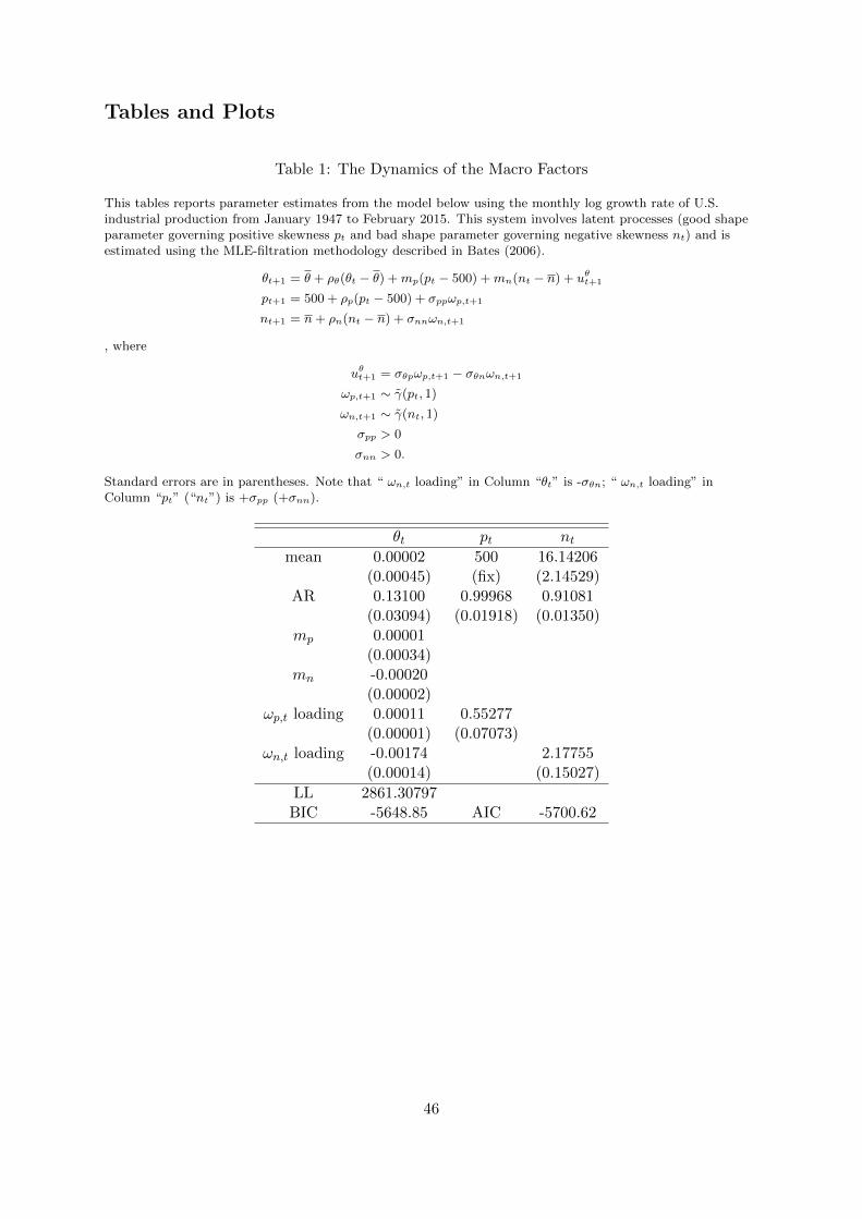
Tables and Plots

Table 1: The Dynamics of the Macro Factors

This tables reports parameter estimates from the model below using the monthly log growth rate of U.S.industrial production from January 1947 to February 2015. This system involves latent processes (good shapeparameter governing positive skewness pt and bad shape parameter governing negative skewness nt) and isestimated using the MLE-filtration methodology described in Bates (2006).

θt+1 = θ + ρθ(θt − θ) +mp(pt − 500) +mn(nt − n) + uθt+1

pt+1 = 500 + ρp(pt − 500) + σppωp,t+1

nt+1 = n+ ρn(nt − n) + σnnωn,t+1

, where

uθt+1 = σθpωp,t+1 − σθnωn,t+1

ωp,t+1 ∼ γ(pt, 1)

ωn,t+1 ∼ γ(nt, 1)

σpp > 0

σnn > 0.

Standard errors are in parentheses. Note that “ ωn,t loading” in Column “θt” is -σθn; “ ωn,t loading” inColumn “pt” (“nt”) is +σpp (+σnn).

θt pt ntmean 0.00002 500 16.14206

(0.00045) (fix) (2.14529)AR 0.13100 0.99968 0.91081

(0.03094) (0.01918) (0.01350)mp 0.00001

(0.00034)mn -0.00020

(0.00002)ωp,t loading 0.00011 0.55277

(0.00001) (0.07073)ωn,t loading -0.00174 2.17755

(0.00014) (0.15027)

LL 2861.30797BIC -5648.85 AIC -5700.62

46

Table 2: The Dynamics of the Corporate Loss Rate

This tables reports parameter estimates for the corporate loss rate model using monthly data from January1982 to February 2015. The mean equation of the loss rate is as follows,

lt+1 = l0 + ρlllt + ρlppt + ρlnnt + σlpωp,t+1 + σlnωn,t+1 + ult+1

ult+1 = σllωl,t+1

ωl,t+1 ∼ γ(vt, 1),

where the variance equation is,

vt+1 = v0 + ρvvvt + σvlωl,t+1.

Teh mean equation is estimated by projection, the variance equation by MLE. Standard errors are inparentheses.

Mean Equationl0 ρll ρlyp ρlyn σlp σln

-0.3463 0.8779 0.0001 0.0047 -0.0004 0.0177(0.0911) (0.0209) (0.0002) (0.0010) (0.0004) (0.0039)

Variance Equationσll v0 ρvv σvl

0.0599 0.8544 0.9051 0.1820(0.0008) (0.1867) (0.0205) (0.0203)

Table 3: Cash Flow Dynamics

Parameters of cash flow processes are shown in Equation (18) for the log earnings growth, Equation (21) for thelog consumption-earnings ratio, Equation (24) for the log dividend-earnings ratio, and Equation (30) for theinflation rate. Estimation is by simple linear projection. Bold (italic) coefficients have <5% (10%) p-values.Robust errors are shown in parentheses. The sample period is 1986/06 to 2015/02 (345 months).

earnings growth log CE log DE inflationgt+1 κt+1 ηt+1 πt+1

drift 0.0285 0.1101 -0.1005 0.0031(0.0273) (0.0453) (0.0337) (0.0014)

AR 0.6619 0.9400 0.9188 0.3973(0.0432) (0.0088) (0.0103) (0.0500)

θt 0.7932 0.8494 1.2237 -0.0718(0.6214) (0.8104) (0.8420) (0.0315)

pt -5.29E-05 4.42E-05 -2.55E-05 -2.07E-06(5.66E-05) (7.10E-05) (7.48E-05) (2.84E-06)

nt -0.0006 0.0049 0.0053 -7.04E-05(0.0004) (0.0005) (0.0006) (1.94E-05)

ωp,t+1 loading -8.63E-05 4.94E-05 5.34E-05 -4.83E-06(1.16E-04) (1.42E-04) (1.46E-04) (5.87E-06)

ωn,t+1 loading -0.0029 0.0061 0.0063 8.27E-05(0.0011) (0.0014) (0.0014) (5.60E-05)

ωl,t+1 loading 0.0010 -0.0014 -0.0014(0.0009) (0.0011) (0.0011)

Gaussian shock volatility 0.0465 0.0568 0.0582 0.0023(0.0018) (0.0021) (0.0022) (0.0001)

Adjusted R2 (conditional mean) 55.58% 98.19% 97.89% 20.58%

47

Table 4: Shock Correlations

ωp,t+1: good uncertainty shock Γ(pt, 1);

ωn,t+1: bad uncertainty shock Γ(nt, 1);

ωl,t+1: loss rate-specific shock Γ(vt, 1);ωg,t+1: log earnings growth-specific shock N(0,1);ωκ,t+1: log C/E-specific shock N(0,1);ωη,t+1: log D/E-specific shock N(0,1);

ωq,t+1: risk aversion-specific shock Γ(qt, 1).

Bold (italic) coefficients have <5% (10%) p-values.The sample period is 1986/06 to 2015/02 (345 months).

ωp ωn ωπ ωl ωg ωκ ωη ωqωp 1 -0.1129 0.0000 -0.0316 0.0000 0.0000 0.0000 0.0000ωn 1 0.0000 0.0246 0.0000 0.0000 0.0000 0.0000ωπ 1 0.0937 0.1083 -0.0215 -0.0604 0.0175ωl 1 0.0000 0.0000 0.0000 0.0788ωg 1 -0.6989 -0.6798 0.0684ωκ 1 0.9882 -0.0283ωη 1 -0.0265ωq 1

Table 5: Financial Instruments Spanning Risk Aversion

This table presents summary statistics of the 6 financial instruments that are used to span our risk aversionmeasure: “tsprd” is the difference between 10-year treasury yield and 3-month Treasury yield; “csprd” is thedifference between Moody’s BAA yield and the 10-year zero-coupon Treasury yield; “DY5yr” is the detrendeddividend yield where the moving average takes the 5 year average of monthly dividend yields, starting one yearbefore; “rvareq” and “rvarcb” are realized variances of log equity returns and log corporate bond returns,calculated from daily returns; “qvareq” is the risk-neutral conditional variance of log equity returns; for theearly years (before 1990), we use VXO and authors’ calculations. Bold (italic) coefficients have <5% (10%)p-values. Block bootstrapped errors are shown in parentheses. The sample period is from 1986/06 to 2015/02(345 months).

tsprd csprd DY5yr rvareq qvareq rvarcbCorrelation Matrix

tsprd 1 0.3524 0.2583 0.1266 0.1240 0.2949csprd 1 0.5063 0.4793 0.5999 0.5340

DY5yr 1 0.1675 0.1641 0.3101rvareq 1 0.8430 0.5942qvareq 1 0.5374rvarcb 1

Summary StatisticsMean 0.0179 0.0231 -0.0030 0.0029 0.0040 0.0002

Boot.SE (0.0006) (0.0004) (0.0003) (0.0003) (0.0002) (1.45E-05)S.D. 0.0116 0.0075 0.0061 0.0059 0.0037 0.0003

Boot.SE (0.0003) (0.0005) (0.0003) (0.0014) (0.0005) (3.86E-05)Skewness -0.2322 1.7891 0.0959 8.1198 3.7225 4.2227Boot.SE (0.0810) (0.2515) (0.1882) (1.5951) (0.5123) (0.6872)AR(1) 0.9669 0.9642 0.9822 0.4311 0.7461 0.5775

SE (0.0137) (0.0143) (0.0083) (0.0489) (0.0360) (0.0442)

48

Table 6: Reduced-Form Risk Aversion Parameters

This table presents the two-step GMM estimation results for risk aversion, , qt = χ′zt, estimated using equitymarket and corporate bond market asset prices. The utility function curvature γ is fixed at 2. The first-stepweight matrix is an identity matrix; the second-step weight matrix builds on the Newey-West spectral densityfunction with 5-month lags, and then is shrunk towards an identity matrix where the shrinkage parameter is0.1. The GMM system also consistently estimates σqq. Therefore, the system has 8 unknown parameters. Thep-value of Hansen’s overidentification test (J test) is calculated from the asymptotic χ2 distribution with thedegree of freedom being 29 (37-8). Bold (italic) coefficients have <5% (10%) p-values. Efficient standard errorsare shown in parentheses. The sample period is 1986/06 to 2015/02 (345 months).

qtEfficient GMM Estimators

constant 0.264(0.510)

χtsprd -0.442(4.507)

χcsprd -7.599(7.186)

χdy5yr 6.550(8.158)

χrvareq -43.232(1.879)

χqvareq 104.599(8.288)

χrvarcb 239.663(114.473)

Correlation with the NBER Indicatorρ(qt, NBERt) 0.397

(0.045)Model Specifications

Hansen’s J 27.919p-value 0.5222

49

Table 7: Structural Risk Aversion Parameters.

This table presents the model-implied risk aversion process parameters. “Projection”: coefficient estimates areobtained from simple projection. “GMM”: the scale parameter of the risk aversion innovation which isestimated in the GMM framework (Table 6). The second and third panels report the variance decompositionresults of the conditional mean and shock structure of qt+1, denotes with“VARC”. In the second panel,V ARC = βx

cov(y,x)var(y)

) where y = Et(qt+1). VARC in the third panel is calculated using the residual,

qt+1 − Et(qt+1). Bold (italic) coefficients have <5% (10%) p-values. Robust and efficient standard errors areshown in parentheses. The sample period is 1986/06 to 2015/02 (345 months).

qt+1 = q0 + ρqq qt + ρqppt + ρqnnt + σqpωp,t+1 + σqnωn,t+1 + uqt+1,

uqt+1 = σqqωq,t+1,

ωq,t+1 = Γ(qt, 1).

Structual Risk Aversion Parameters, qt+1

◦ Projection ◦ GMMConstant pt nt qt ωp,t+1 ωn,t+1 ωq,t+1

Est -0.1040 0.0006 0.0056 0.6293 0.0004 -0.0009 0.1211(SE) (0.0835) (0.0002) (0.0010) (0.0412) (0.0004) (0.0034) (0.0067)

Conditional Mean Variance Decomposition (60.70% of Total Variance)pt nt qt

VARC 77.15% 1.68% 21.17%

Shock Structure Variance Decomposition (39.30% of Total Variance)ωp,t+1 ωn,t+1 ωq,t+1

VARC 0.35% 0.30% 99.35%

Table 8: Fit of Moments.

This table evaluates the fit of conditional moments of equity and corporate bond returns. That is, Column“Model” reports the averages of the relevant model-implied conditional moments. The “Empirical Averages”represent the sample averages of the excess returns (for “Mom 1” and “Mom 4”), the sample average ofempirical conditional variances (for “Mom 2”, “Mom 3”, and “Mom 5”). In “Mom 6” and “Mom 7”, “RiskAversion Innovation” is uqt+1 in Equation (27). The variance and unscaled skewness rows compare the averagemodel-implied conditional moments with the unconditional moments. Bolded number(s) denote a distance ofless than 1.645 standard errors from the corresponding point estimate, and italicized number(s) a distance ofmore than 1.645 but less than 1.96 standard errors. Block bootstrapped standard errors are shown inparentheses; we allow the block size to vary for different moments, block sizes=[0 6 15 1 10] for Mom 1 to Mom5, respectively. Asymptotic standard errors (standard deviation divided by square root of the number ofobservations) are reported for Mom 6 and Mom 7. The sample period is 1986/06 to 2015/02 (345 months).

Moment Model Empirical Average Boot.SE/SEMom 1 Equity Risk Premium 0.00749 0.00530 (0.00246)Mom 2 Equity Physical Variance 0.00310 0.00286 (0.00051)Mom 3 Equity Risk-neutral Variance 0.00369 0.00397 (0.00049)Mom 4 Corporate Bond Risk Premium 0.00289 0.00388 (0.00050)Mom 5 Corporate Bond Physical Variance 0.00027 0.00024 (0.00003)Mom 6 Risk Aversion Innovation Variance 0.00823 0.00906 (0.00215)Mom 7 Risk Aversion Innovation Unscaled Skewness 0.00246 0.00246 (0.00134)

50

Table 9: Asset Prices and the State Variables.

The asset conditional moments are explained by {pt, nt, vt, qt}. The coefficients are scaled by the standarddeviation of the state variable in the same column, and then multiplied by 10000 for reporting purposes. VARCis coefficient*Cov(xt,Momt)

V ar(Momt)where x ∈ {p, n, v, q} and Mom is from Mom 1 to Mom 5. The variance

decomposition is reported in a bold italic font.

Model-implied coefficients of moments on state variables {pt, nt, vt, qt}Moment pt nt vt qt

Mom 1 Equity Risk Premium 0.1286 4.6231 0.0039 54.0505VARC 0.014% 4.449% 0.000% 95.537%

Mom 2 Equity Physical Variance 0.0651 2.5845 0.0006 5.5008VARC -0.031% 26.640% 0.000% 73.391%

Mom 3 Equity Risk-neutral Variance 0.0652 2.5454 0.0006 11.2064VARC 0.011% 12.646% 0.000% 87.343%

Mom 4 Corporate Bond Risk Premium 0.0752 7.6016 -0.0200 3.8662VARC -0.143% 71.227% -0.001% 28.918%

Mom 5 Corporate Bond Physical Variance 0.0009 0.3137 0.0007 0.0015VARC -0.090% 99.865% -0.001% 0.226%

Table 10: Predicting Realized Excess Returns and Variances.

This table reports the regression coefficients of realized excess returns and realized variances of equity andcorporate bond. The coefficients are scaled by the standard deviation of the state variable in the same row, andthen multiplied by 100 for reporting purposes. “Model-Implied Moments” are risk premiums (for realized excessreturns) and physical variances (for realized variances). Bold (italic) coefficients have <5% (10%) p-values. TheR2 is adjusted. Standard errors are shown in parentheses. The sample period is 1986/06 to 2015/02 (345months).

reqt+1 − rft RV AReqt+1 rcbt+1 − rft RV ARcbt+1

pt -0.1648 0.0190 -0.1098 -0.0003(0.2584) (0.0312) (0.0922) (0.0014)

nt -1.2623 0.1695 0.0044 0.0093(0.2928) (0.0354) (0.1045) (0.0016)

vt -0.3478 0.0410 -0.1089 -0.0029(0.2359) (0.0285) (0.0842) (0.0013)

qt 0.6562 0.1047 0.1262 0.0036(0.1866) (0.0226) (0.0666) (0.0010)

Model-Implied Moments 0.6671 3.8517 1.6610 3.8195(0.4018) (0.4017) (0.8376) (0.4250)

Corr w/ NBER 0.45 0.54 0.61 0.65R2 5.6% 0.1% 21.8% 21.0% 1.2% 0.8% 22.0% 18.9%

51

Table 11: Out-Of-Sample Exercise.

This table analyzes in-sample (see Section 3.3) and out-of-sample risk premium estimates of equity returns andcorporate bond returns. “Realized” indicates the realized excess returns. “Mod (1)” indicates the in-sample(full-sample) estimates of model-implied risk premiums, the dynamics of which are determined by{pt, nt, vt, qt}. “Mod (2)” indicates the out-of-sample estimates of model-implied risk premiums. Define a60-month rolling window from t− 60 to t− 1, then project one-period ahead excess returns on the 4 statevariables, use the coefficient estimates to obtain Et(rt+1 − rft), repeat. We also consider three out-of-sampleempirical models that use three instruments sets (subsets of zt), respectively: (1) dividend yield, (2) dividedyield + term spread + credit spread, (3) physical uncertainty plus variance risk premium estimate. The tablethen reports the optimal combination of Mod and Emp Mod estimate. Least Square standard errors are shownin parentheses. Bold (italic) coefficients have <5% (10%) p-values. R2 is adjusted. The (full) sample period is1986/06 to 2015/02 (345 months).

Least-Square Estimate of a inrt+1 − rft = a×Mod(t, i) + (1− a)× Emp Mod(t, j) + et+1

i = 1, 2; j = 1, 2, 3

◦ Equity: ◦ Corporate Bond:Mod (1) Mod (2) Mod (1) Mod (2)

Emp Mod (1) 0.8262 0.4843 1.0155 0.2553(0.1095) (0.0995) (0.1365) (0.1161)

Emp Mod (2) 0.9613 0.6618 0.8236 0.4748(0.0934) (0.0870) (0.0841) (0.0903)

Emp Mod (3) 0.8305 0.6216 0.9238 0.4719(0.0810) (0.0801) (0.1090) (0.0903)

Table 12: Uncertainty Index.

This table presents regression results of the filtered macroeconomic uncertainty (from industrial productiongrowth) on the set of instruments used to determine risk aversion. “Total” is the total industrial productiongrowth variance, which is a function of pt and nt, σ

2θppt + σ2

θnnt. “×103” in the header means that thecoefficients and their SEs reported are multiplied by 1000 for reporting convenience. Bold (italic) coefficientshave <5% (10%) p-values. Robust and efficient standard errors are shown in parentheses. The R2 is adjusted.The sample period is 1986/06 to 2015/02 (345 months).

(×103) (×103) (×103)Total VARC Upside VARC Downside VARC

constant -0.006 0.006 -0.012(0.005) (0.000) (0.005)

χtsprd -0.573 -2.38% -0.005 5.21% -0.568 -2.54%(0.112) (0.002) (0.113)

χcsprd 1.919 61.33% -0.006 4.05% 1.925 60.98%(0.246) (0.005) (0.247)

χDY 5yr 1.083 19.83% -0.063 84.69% 1.146 21.21%(0.234) (0.005) (0.235)

χrvareq -0.318 -4.81% -0.022 -0.41% -0.296 -4.39%(0.399) (0.008) (0.401)

χqvareq 1.243 14.28% 0.066 8.08% 1.177 13.24%(0.673) (0.014) (0.676)

χrvarcb 14.829 11.76% 0.158 -1.61% 14.671 11.49%(5.910) (0.124) (5.933)

R2 47.72% 44.35% 47.95%

52

Table 13: On the Predictive Power of Risk Aversion Index and Uncertainty Index on FutureOutput Growth.

This table reports the coefficient estimates of the following predictive regression,

θt+k = a+ b′xt + rest+k, (C.1)

where θt+k represents future industrial production growth during period t+ 1 and t+ k (∑kτ=1 θt+τ ) and xt

represents a vector of current predictors. We consider (1) our risk aversion index raBEX , (2) our uncertaintyindex uncBEX (financial proxy), (3) the risk-neutral conditional variance (the square of the month-end VIX(after 1990) / VXO (prior to 1990) index divided by 120000), QV AR, and (4) the true total macroeconomicuncertainty filtered from industrial production index unctrue. The coefficients are scaled by the standarddeviation of the predictor in the same column for reporting purposes. Hodrick (1992) standard errors arereported in parentheses, and adjusted R2s are in %. Bold (italic) coefficients have <5% (10%) p-values.

raBEX uncBEX QV AR unctrue

A. Univariate1m -0.002 -0.003 -0.002 -0.002

(0.001) (0.000) (0.001) (0.001)7.9% 19.2% 6.5% 12.9%

1q -0.005 -0.008 -0.005 -0.007(0.001) (0.001) (0.002) (0.001)13.9% 34.9% 15.3% 26.3%

4q -0.006 -0.016 -0.008 -0.010(0.003) (0.004) (0.003) (0.004)2.0% 15.2% 3.7% 6.2%

B. Multivariate (1) R2

1m 0.000 -0.003 0.001 19.4%(0.001) (0.001) (0.000)

1q 0.002 -0.008 -0.001 35.3%(0.001) (0.001) (0.001)

4q 0.013 -0.021 -0.005 18.4%(0.002) (0.005) (0.002)

C. Multivariate (2) R2

1m 0.000 -0.002 0.001 -0.001 19.1%(0.001) (0.000) (0.000) (0.001)

1q 0.002 -0.006 -0.001 -0.003 36.7%(0.001) (0.001) (0.001) (0.001)

4q 0.013 -0.022 -0.005 0.001 17.4%(0.002) (0.005) (0.002) (0.003)

53

Table 14: Alternative Risk Aversion and Uncertainty Measures.

This table report the correlation between our risk aversion and economic uncertainty indices and existingmeasures. For risk aversion (Panel A), we consider three categories. A.1) We follow Wachter (2006) to create afundamental risk aversion process from inflation-adjusted (real) quarterly consumption growth (

∑4 0j=0∆ct−j);A.2) we consider the well-known sentiment index by Baker and Wurgler (2006) from the behavior financeliterature, and the Michigan Consumer Sentiment Index (that directly measures the consumer sentiment); A.3)we also consider an industry index, the Credit Suisse First Boston Risk Appetite Index. For economicuncertainty (Panel B), we consider B.1) the macroeconomic uncertainty index created by Jurado, Ludvigson,and Ng (2015), and B.2) the Economic Policy Uncertainty Index created by Baker, Bloom, and Davis (2016).Correlations are calculated using overlapping samples at the monthly frequency. Standard errors are shown inparentheses. Bold correlation coefficients have <5% p-values.

A. Correlations with Extant Risk Aversion IndicesA.1) “Fundamental” Habit Model:Wachter (2006) / Campbell and Cochrane (1999) 0.1228A.2) Sentiment Index: (0.0536)Baker and Wurgler (2006) -0.1554

(0.0533)Michigan Consumer Sentiment Index -0.2603

(0.0521)A.3) Industry Index -0.4770Credit Suisse First Boston Risk Appetite Index (0.0475)

B. Correlations with Extant Uncertainty IndicesB.1) Macroeconomic Uncertainty:Jurado, Ludvigson, and Ng (2015) 0.8003

(0.0324)B.2) Political Uncertainty:Baker, Bloom, and Davis (2016) 0.3438

(0.0507)

Table 15: Market Integration Test.

This table tests market integration by evaluating the fit of Treasury bond return moments priced using thepricing kernel extracted from risky assets. Column “Model” reports the averages of the relevant model-impliedconditional moments. The “Empirical Averages” represent the sample averages of the excess returns (“Mom1”), the sample average of empirical conditional variances (“Mom 2”, “Mom 3”). Bolded number(s) denote adistance of less than 1.645 standard errors from the corresponding point estimate, and italicized number(s) adistance of more than 1.645 but less than 1.96 standard errors. Block bootstrapped standard errors are shownin parentheses; we allow the block size to vary for different moments, block sizes=[0 14 13] for Mom 1 to Mom3, respectively. The sample period is 1986/06 to 2015/02 (345 months).

Moment Model Empirical Average Boot.SEMom 1 Treasury Bond Risk Premium -0.00366 0.00285 (0.00117)Mom 2 Treasury Bond Physical Variance 0.00111 0.00035 (0.00004)Mom 3 Treasury Bond Risk-neutral Variance 0.00113 0.00043 (0.00003)

54

194701 195504 196308 197112 198004 198808 199612 200504 201308-0.04

-0.02

0

0.02

0.04

0.06conditional mean

194701 195504 196308 197112 198004 198808 199612 200504 2013080

500

1000

pt

194701 195504 196308 197112 198004 198808 199612 200504 2013080

20

40

60

80

nt

Figure 1: Filtered state variables extracted from industrial production growth. The shadedregions are NBER recession months from the NBER website.

55

194701 195504 196308 197112 198004 198808 199612 200504 2013080

0.005

0.01

0.015

conditional volatility

194701 195504 196308 197112 198004 198808 199612 200504 201308

-0.6

-0.4

-0.2

0conditional scaled skewness

Figure 2: Model-implied conditional moments for industrial production growth. The shadedregions are NBER recession months from the NBER website.

56

198202 198603 199005 199407 199809 200211 200701 201103 201502

-3

-2

-1

Model-implied conditional mean of the loss rate, Et[lt+1]

conditional mean

E(lt+1) = !2:2237

198202 198603 199005 199407 199809 200211 200701 201103 201502

0.15

0.2

0.25

Model-implied conditional volatility of the loss rate, V olt[lt+1]

conditional volatility

V ol(lt+1 ! E(lt+1)) = 0:1856

198202 198603 199005 199407 199809 200211 200701 201103 201502

0.4

0.5

0.6

0.7

0.8

Model-implied conditional skewness of the loss rate, Skewt[lt+1]

conditional skewness

Skew(lt+1 ! E(lt+1)) = 0:6269

198202 198603 199005 199407 199809 200211 200701 201103 201502

6

8

10

12

Model-implied loss rate shcok shape parameter, vt

Figure 3: Conditional moments of the loss rate. The shaded regions are NBER recession monthsfrom the NBER website.

57

198202 198603 199005 199407 199809 200211 200701 201103 2015020

0.1

0.2

0.3

0.4

0.5

0.6

0.7

0.8

0.9

1Loss rate conditional variance decomposition

pt

nt

vt

vt(emp) = 94:74%

Figure 4: Decomposition of the conditional variance of the loss rate. The shaded regions areNBER recession months from the NBER website. The green dashed line depicts the ratio of theunconditional variance of ult+1 to the unconditional variance of the total loss rate disturbance,or 1-R2 from the projection.

58

198606 199007 199409 199811 200301 200703 201105 2015020

0.005

0.01

0.015

0.02

0.025

0.03EmpiricalModel

Figure 5: Model-implied and empirical risk-neutral conditional variances of equity market re-turns. The shaded regions are NBER recession months from the NBER website.

198606 199007 199409 199811 200301 200703 201105 201502

3

4

5

6

7

8

9

10

11

12

Figure 6: The Time Variation in the Risk Aversion. Risk aversion is γ exp(qt). The shadedregions are the NBER recession months from the NBER website.

59

198606 199007 199409 199811 200301 200703 201105 201502

Ris

k A

vers

ion

Inde

x

0

2

4

6

8

10

12

Unc

erta

inty

Inde

x

#10-4

0

1

2

Figure 7: Risk aversion index (solid blue/left y-axis) and Uncertainty index (dashed red/righty-axis). According to Section 4, both the risk aversion index denoted as raBEX = γ exp(qt) andthe uncertainty index denoted as uncBEX are functions of a set of financial instruments. SeeEquations (49) and (59). Correlation between the two series is 67.94%. The shaded regions areNBER recession months from the NBER website.

60

Figure 8: qt and Uncertainty Index at Daily Frequency Around the Bear Stearns and LehmanBrothers Collapses in 2008. We calculate and plot our daily indices one month before and afterthe collapses.

61