Embed Size (px)
Citation preview
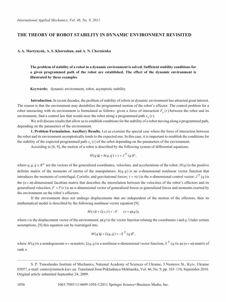
THE THEORY OF ROBOT STABILITY IN DYNAMIC ENVIRONMENT REVISITED
À.À. Martynyuk, A. S. Khoroshun, and A. N. Chernienko
The problem of stability of a robot in a dynamic environment is solved. Sufficient stability conditions for
a given programmed path of the robot are established. The effect of the dynamic environment is
illustrated by three examples
Keywords: dynamic environment, robot, asymptotic stability
Introduction. In recent decades, the problem of stability of robots in dynamic environment has attracted great interest.
The reason is that the environment may destabilize the programmed motion of the robot’s effector. The control problem for a
robot interacting with its environment is formulated as follows: given a force of interaction F tr
( ) between the robot and its
environment, find a control law that would steer the robot along a programmed path x tr
( ).
We will discuss results that allow us to establish conditions for the stability of a robot moving along a programmed path,
depending on the parameters of the environment.
1. Problem Formulation. Auxiliary Results. Let us examine the special case where the force of interaction between
the robot and its environment asymptotically tends to the expected one. In this case, it is important to establish the conditions for
the stability of the expected programmed path x tr
( ) of the robot depending on the parameters of the environment.
According to [6, 9], the motion of a robot is described by the following system of differential equations:
H q q h q q J q F( )�� ( , � ) ( )� � ��T
,
where q q, �, ��q Rn
� are the vectors of the generalized coordinates, velocities, and accelerations of the robot; H q( ) is the positive
definite matrix of the moments of inertia of the manipulators; h q q( , � ) is an n-dimensional nonlinear vector function that
introduces the moments of centrifugal, Coriolis, and gravitational forces; � �� ( )t is the n-dimensional control vector; J qT
( ) is
the (n m� )-dimensional Jacobian matrix that describes the interrelation between the velocities of the robot’s effectors and its
generalized velocities; F F t� ( ) is an n-dimensional vector of generalized forces or generalized forces and moments exerted by
the environment on the robot’s effectors.
If the environment does not undergo displacements that are independent of the motion of the effectors, then its
mathematical model is described by the following nonlinear vector equation [9]:
M s s L s s F( )�� ( , � )� � � ( ( ))s q� � ,
where s is the displacement vector of the environment; �( )q is the vector function relating the coordinates s and q. Under certain
assumptions, [9] this equation can be rearranged into
M q q L q q S q F( )�� ( , � ) ( )� � �T
,
where M q( ) is a nondegenerate n m� -matrix; L q q( , � ) is a nonlinear n-dimensional vector function; S qT
( ) is an (n m� )-matrix of
rank n.
International Applied Mechanics, Vol. 46, No. 9, 2011
1056 1063-7095/11/4609-1056 ©2011 Springer Science+Business Media, Inc.
S. P. Timoshenko Institute of Mechanics, National Academy of Sciences of Ukraine, 3 Nesterov St., Kyiv, Ukraine
03057, e-mail: [email protected]. Translated from Prikladnaya Mekhanika, Vol. 46, No. 9, pp. 103–110, September 2010.
Original article submitted September 24, 2009.
Thus, the set of systems of equations that describe the motion of the robot and the behavior of its environment represents
a mathematical model of a robot in an environment.
According to [4, 6, 10], this set of systems of differential equations can be reduced to one vector differential equation:
dx dt A t x t x t x t/ ( ) ( , ) ( , ) ( )� � �� , x t x( )0 0
� , (1)
where x t Rn
( )� is the state vector of the robot at time t R��
; A t( ) is a matrix and �( , )t x , ( , ) ( )t x t are vector functions. The
robot moving in its environment is analyzed for stability by simultaneously solving Eq. (1) and the equation
d dt Q t F t F t / ( ) ( ( ) ( ) ( ))� � �r
(2)
under certain assumptions on the functions describing the effect of the environment on the robot.
Following [6], we make the following assumptions:
(i) the vector function �( , )t x appearing in Eq. (1) is such that for each L � 0there exist D D L� ( )and T T L� ( )such that
| | ( , )| | | | | |� t x L x� for | | | |x D� and t T ;
(ii) the vector function that describes the effect of the environment on the robot, u t x( , ) � ( , ) ( )t x t , satisfies the
condition u t x( , ) � 0 as t � � uniformly in x for rather small | | | |x , this condition corresponding to a control such that which
F t F t( ) ( )�r
as t � ��;
(iii) the matrix function A t( ) can be represented in the form A t A B t( ) ( )� � , where A is a constant matrix with all its
eigenvalues satisfying the condition Re( ( ))� �i
A � � � 0, i � 1, � ,n, and the matrix function B t( ) is such that | | ( )| |B t � 0 as
t � �;
(iv) the matrix function A t( ) can be represented in the form A t A B t( ) ( )� � , where A is a constant matrix with all its
eigenvalues satisfying the condition Re( ( ))� �i
A � � � 0, i � 1,� ,n, and the matrix function B t( )is such that there exist c � 0such
that | | ( )| |B t c� for all t R��
.
Theorem 1. Let assumptions (i)–(iii) be valid for Eqs. (1) and (2). Then there exists t R0
��
such that any motion x t( ,
t x0 0
, ) of the robot described by system (1) tends to 0 as t � � for rather small | | ( )| |x t0
.
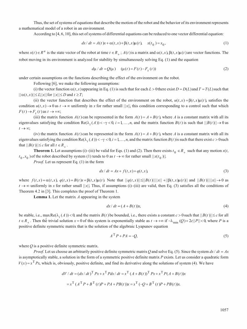
Proof. Let us represent Eq. (1) in the form
dx dt Ax f t x q t x/ ( , ) ( , )� � � , (3)
where f t x t x( , ) ( , )� � , q t x B t x t x t( , ) ( ) ( , ) ( )� � . Note that | | ( , )| | | | ( )| | | | | |q t x B t x� �| | ( , ) ( )| | t x t and | | ( )| | | | | |B t x � 0 as
t � � uniformly in x for rather small | | | |x . Thus, if assumptions (i)–(iii) are valid, then Eq. (3) satisfies all the conditions of
Theorem 4.2 in [3]. This completes the proof of Theorem 1.
Lemma 1. Let the matrix A appearing in the system
dx dt A B t x/ ( ( ))� � , (4)
be stable, i.e., max ( ( ))i
iARe � � 0, and the matrix B t( ) be bounded, i.e., there exists a constant c � 0 such that | | ( )| |B t c� for all
t R��
. Then the trivial solution x � 0 of this system is exponentially stable as t � �� if � � ��min
( ) | | | |Q c P2 0, where P is a
positive definite symmetric matrix that is the solution of the algebraic Lyapunov equation
A P PA QT
� � � , (5)
where Q is a positive definite symmetric matrix.
Proof. Let us choose an arbitrarily positive definite symmetric matrix Q and solve Eq. (5). Since the system dx dt Ax/ �
is asymptotically stable, a solution in the form of a symmetric positive definite matrix P exists. Let us consider a quadratic form
V x x Px( ) �T
, which is, obviously, positive definite, and find its derivative along the solutions of system (4). We have
dV dt dx dt Px x Pdx dt x A B t Px x P A B t/ ( / ) / ( ( )) ( ( )� � � � � �T T T T T
)x
� � � � � � � �x A P B t P PA PB t x x Q B t P PB t xT T T T T
( ( ) ( )) ( ( ) ( )) .
1057
Then dV dt Q c P x W x/ ( ( ) | | | | ) | | | | ( )min
� � � �� 22
for all t R��
and all x R� , where | | | | ( )/
x x x�T 1 2
is a Euclidean
vector norm, and | | | |P is a spectral matrix norm; W x( ) � x BxT
is a negative definite quadratic form; B Q c P I� � �( ( ) | | | | )min
� 2 ,
where I is a unit matrix. According to the theorem from [1, p. 252], the trivial solution x � 0of system (4) is exponentially stable
as t � ��. The lemma is proved.
Theorem 2. Let system (1) be such that assumptions (i), (ii), (iv) and the conditions � � ��min
( ) | | | |Q c P2 0 are valid,
where P is a positive definite symmetric matrix that is a solution of the algebraic Lyapunov equation A P PA QT
� � � , whereQ is
a positive definite symmetric matrix. Then the trivial solution x � 0of the system dx dt A t x t x/ ( ) ( , )� � � is stable under constant
perturbations.
Proof. According to Lemma 1, the trivial solution x � 0 of system (4) is exponentially stable, which is proved by a
Lyapunov functionV x x Px( ) �T
. It is obvious thatV x( )is a Lyapunov function proving that the trivial solution x � 0of the system
dx dt A t x t x/ ( ) ( , )� � � is asymptotically stable in some neighborhood of 0.
Since �V x( ) is obviously bounded in the neighborhood of zero,V x x Px( ) �T
satisfies Malkin’s stability theorem [2].
Theorem 2 is proved.
Remark. The inequality � � ��min
( ) | | | |Q c P2 0can be used to find c � 0such that the trivial solution x � 0of system (4) is
exponentially stable as t � �� and the trivial solution x � 0 of the system dx dt A t x t x/ ( ) ( , )� � � is stable under constant
perturbations.
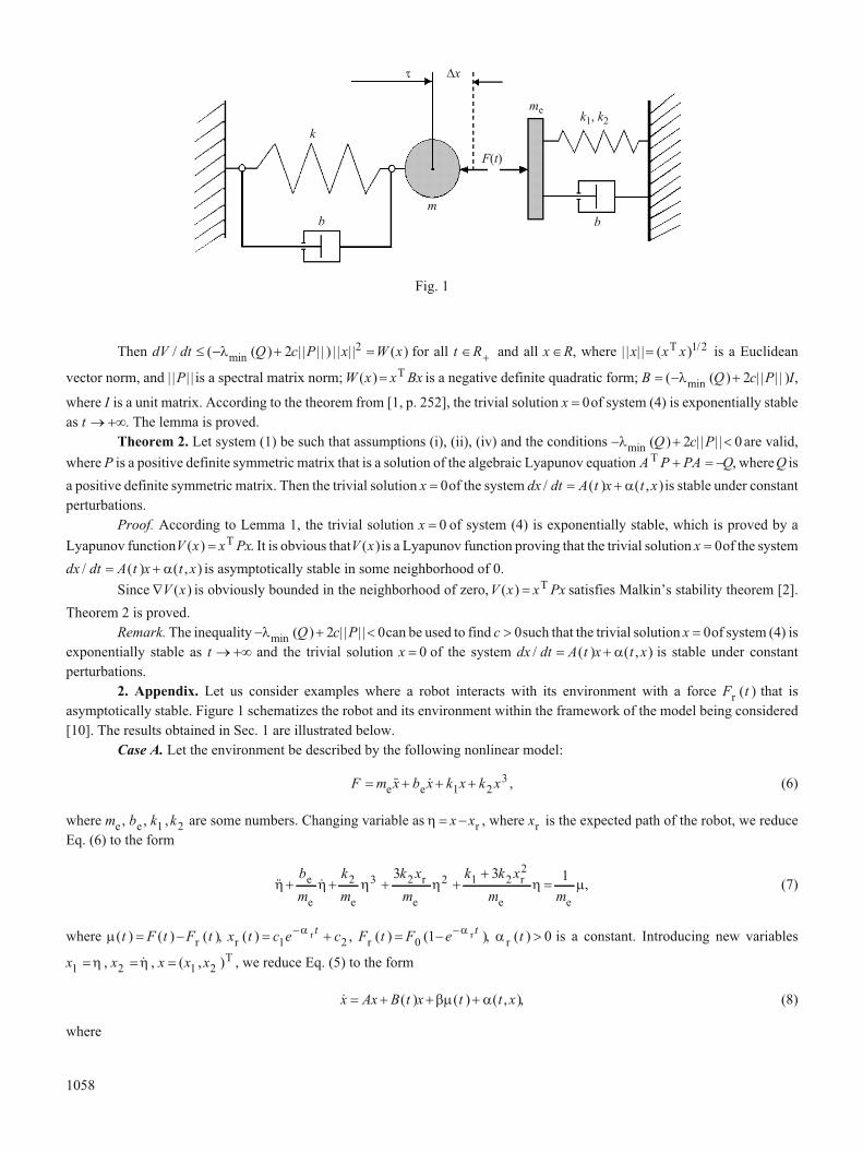
2. Appendix. Let us consider examples where a robot interacts with its environment with a force F tr
( ) that is
asymptotically stable. Figure 1 schematizes the robot and its environment within the framework of the model being considered
[10]. The results obtained in Sec. 1 are illustrated below.
Case À. Let the environment be described by the following nonlinear model:
F m x b x k x k x� � � �e e�� �
1 2
3, (6)
where me, b
e, k k
1 2, are some numbers. Changing variable as � � �x x
r, where x
ris the expected path of the robot, we reduce
Eq. (6) to the form
�� �� � � � � � � � �
�
�
b
m
k
m
k x
m
k k x
m m
e
e e
r
e
r
e e
2 3 2 2 1 2
23 3 1
, (7)
where ( ) ( ) ( )t F t F t� �r
, x t c e ct
rr( ) � �
�
1 2
�, F t F e
t
rr( ) ( )� �
�
01
�, �
r( )t � 0 is a constant. Introducing new variables
x1
� � , x2
� �� , x x x� ( , )1 2
T, we reduce Eq. (5) to the form
� ( ) ( ) ( , )x Ax B t x t t x� � � � � , (8)
where
1058
Fig. 1
b
�
k1, k2
me
F(t)
b
m
k
�x
A k k c
m
b
m
B t k c c e��
�
�
�
�
�
�
�
�
�
�
�
�
��
�
0 1
3
0 0
61 2 2
2
2 1 2
e
e
e
, ( )�
r r
e
t tk c e
m
�
�
�
�
�
�
�
�
�
�
�
�3
02 1
2 2�
,
��
�
�
�
�
�
�
�
��
� �
�
�
�
��
�
�
�
0
1
0
32
1
2 2
1
3
m
t xk x
mx
k
mx
e
r
e e
, ( , )��
,
k k m b1 2
, , ,e e
are positive constants. It is easy to verify that the matrix A is stable, i.e., max ( ( ))i
iARe � � 0. Since the interaction
force asymptotically tends to the expected one, we assume that | | ( )| | t � 0as t � � uniformly in x. Note also that | | ( )| |B t � 0
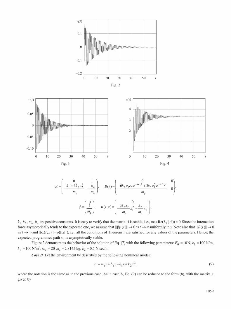
as t � � and | | ( , )| | (| | | | )� t x o x� , i.e., all the conditions of Theorem 1 are satisfied for any values of the parameters. Hence, the
expected programmed path xr
is asymptotically stable.
Figure 2 demonstrates the behavior of the solution of Eq. (7) with the following parameters: F0
10� N, k1
100� N/m,
k2
100� N/m3, �
r� 20, m
e� 2.8145 kg, b
e� 0.5 N�señ/m.
Case B. Let the environment be described by the following nonlinear model:
F m x b x k x k x� � � �e e�� �
1 2
3, (9)
where the notation is the same as in the previous case. As in case A, Eq. (9) can be reduced to the form (8), with the matrix A
given by
1059
Fig. 2
� �(t
–0.2
0
–0.1
0.1
0 10 20 30 40 50 t
Fig. 3 Fig. 4
� �(t
–0.10
0
0 10 20 30 40 50 t 0 10 20 30 40 50 t
–0.05
0.05
4
2
3
1
� �(t
A k k c
m
b
m
� �
�
�
�
�
�
�
�
�
�
�
�
0 1
31 2 2
2
e
e
e
.
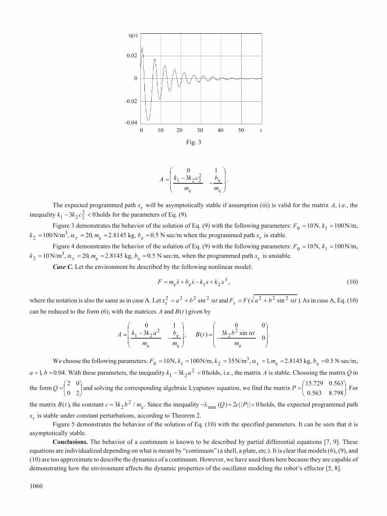
The expected programmed path xr
will be asymptotically stable if assumption (iii) is valid for the matrix A, i.e., the
inequality k k c1 2 2
23 0� � holds for the parameters of Eq. (9).
Figure 3 demonstrates the behavior of the solution of Eq. (9) with the following parameters: F0
10� N, k1
100� N/m,
k2
100� N/m3, �
r� 20, m
e� 2.8145 kg, b
e� 0.5 N�señ/m when the programmed path x
ris stable.
Figure 4 demonstrates the behavior of the solution of Eq. (9) with the following parameters: F0
10� N, k1
100� N/m,
k2
10� N/m3, �
r� 20, m
e� 2.8145 kg, b
e� 0.5 N�señ/m, when the programmed path x
ris unstable.
Case C. Let the environment be described by the following nonlinear model:
F m x b x k x k x� � � �e e�� �
1 2
3, (10)
where the notation is also the same as in case A. Let x a b tr
2 2 2 2� � sin � and F F a b t
r� �( sin )
2 2 2� . As in case A, Eq. (10)
can be reduced to the form (6), with the matrices A and B t( ) given by
A k k a
m
b
m
B t k b t
m
� �
�
�
�
�
�
�
�
�
�
�
�
��
0 1
3
0 0
31 2
2
2
2
e
e
e e
, ( ) sin �
0
�
�
�
�
�
�
�
�
�
�
.
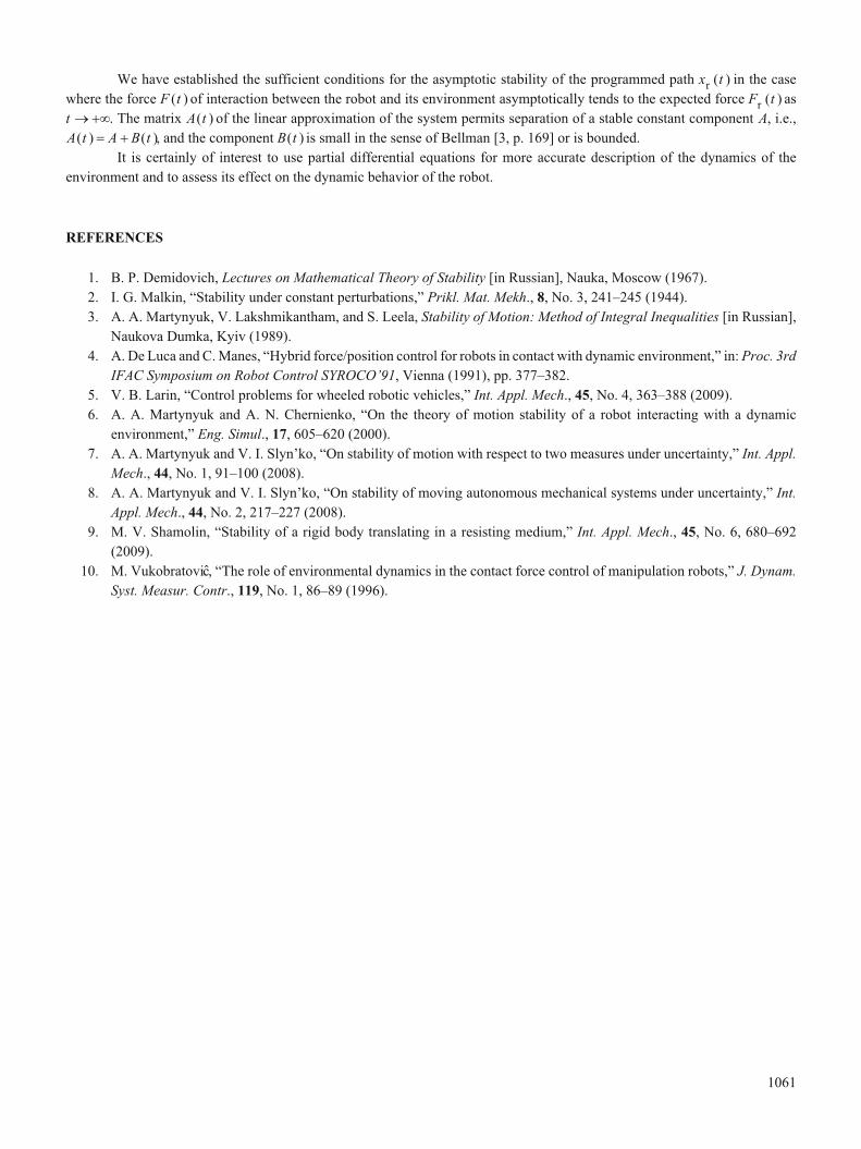
We choose the following parameters: F0
10� N, k1
100� N/m, k2
35� N/m3, �
r� 1, m
e�2.8145 kg, b
e�0.5 N�señ/m,
a � 1, b � 0.04. With these parameters, the inequality k k a1 2
23 0� � holds, i.e., the matrix A is stable. Choosing the matrix Q in
the form Q ��
�
�
�
�
�
2 0
0 2and solving the corresponding algebraic Lyapunov equation, we find the matrix P �
�
�
�
�
�
�
15 729 0 563
0 563 8 798
. .
. .. For
the matrix B t( ), the constant c k b m� 32
2/
e. Since the inequality � � ��
min( ) | | | |Q c P2 0 holds, the expected programmed path
xr
is stable under constant perturbations, according to Theorem 2.
Figure 5 demonstrates the behavior of the solution of Eq. (10) with the specified parameters. It can be seen that it is
asymptotically stable.
Conclusions. The behavior of a continuum is known to be described by partial differential equations [7, 9]. These
equations are individualized depending on what is meant by “continuum” (a shell, a plate, etc.). It is clear that models (6), (9), and
(10) are too approximate to describe the dynamics of a continuum. However, we have used them here because they are capable of
demonstrating how the environment affects the dynamic properties of the oscillator modeling the robot’s effector [5, 8].
1060
Fig. 3
� �(t
–0.04
0
–0.02
0.02
0 10 20 30 40 50 t
We have established the sufficient conditions for the asymptotic stability of the programmed path x tr
( ) in the case
where the force F t( ) of interaction between the robot and its environment asymptotically tends to the expected force F tr
( ) as
t � ��. The matrix A t( ) of the linear approximation of the system permits separation of a stable constant component A, i.e.,
A t A B t( ) ( )� � , and the component B t( ) is small in the sense of Bellman [3, p. 169] or is bounded.
It is certainly of interest to use partial differential equations for more accurate description of the dynamics of the
environment and to assess its effect on the dynamic behavior of the robot.
REFERENCES
1. B. P. Demidovich, Lectures on Mathematical Theory of Stability [in Russian], Nauka, Moscow (1967).
2. I. G. Malkin, “Stability under constant perturbations,” Prikl. Mat. Mekh., 8, No. 3, 241–245 (1944).
3. A. A. Martynyuk, V. Lakshmikantham, and S. Leela, Stability of Motion: Method of Integral Inequalities [in Russian],
Naukova Dumka, Kyiv (1989).
4. A. De Luca and C. Manes, “Hybrid force/position control for robots in contact with dynamic environment,” in: Proc. 3rd
IFAC Symposium on Robot Control SYROCO’91, Vienna (1991), pp. 377–382.
5. V. B. Larin, “Control problems for wheeled robotic vehicles,” Int. Appl. Mech., 45, No. 4, 363–388 (2009).
6. A. A. Martynyuk and A. N. Chernienko, “On the theory of motion stability of a robot interacting with a dynamic
environment,” Eng. Simul., 17, 605–620 (2000).
7. A. A. Martynyuk and V. I. Slyn’ko, “On stability of motion with respect to two measures under uncertainty,” Int. Appl.
Mech., 44, No. 1, 91–100 (2008).
8. A. A. Martynyuk and V. I. Slyn’ko, “On stability of moving autonomous mechanical systems under uncertainty,” Int.
Appl. Mech., 44, No. 2, 217–227 (2008).
9. M. V. Shamolin, “Stability of a rigid body translating in a resisting medium,” Int. Appl. Mech., 45, No. 6, 680–692
(2009).
10. M. Vukobratovi�c, “The role of environmental dynamics in the contact force control of manipulation robots,” J. Dynam.
Syst. Measur. Contr., 119, No. 1, 86–89 (1996).
1061