The Theory of Markets - · PDF file(holding other things constant) ... LOCATION of the Demand curve (way to the right or way to the left) ... causing the supply curve to shift up

Copyright © 2011 Pearson Addison-Wesley. All rights reserved.

Chapter 7 The Theory of Markets

Copyright © 20011Pearson Addison-Wesley. All rights reserved. 7-2

•  Demand (from Consumers) and Supply (from Producers) interact in the market place

•  Examples of markets: –  Supermarket: market for food and household items

•  Supermarkets supply goods, consumers demand goods

–  Stock market: market for previously issued stocks –  Labor market: classified ads, word of mouth, that make up

the supply and demand for labor •  Here, workers supply labor and firms demand labor

Demand, Supply and Markets

Copyright © 2011 Pearson Addison-Wesley. All rights reserved. 7-3

•  A market is not a 'place', –  It is an interaction between buyers (Demand) and

sellers (Supply) •  The interaction of supply and demand

determines the 'equilibrium' price and quantity of goods and resources

What is a market?


•  Assumptions behind consumer demand: •  Consumers are rational •  Consumers prefer more to less •  Consumers can rank goods according to how much they

are worth to them at various prices •  Consumers have a limited budget •  No 1 Consumer can influence the price (many buyers)

Demand: the desire to purchase a good or service


•  Then they could control it and the demand curve would not be fixed (it would vary with the large consumer’s actions) – Like Wal-Mart buying drugs for resale:

•  They tell pharmaceutical companies: give us a lower price or else we won't stock your product

•  Which then allows Wal-Mart to drive local pharmacies out of business

•  The supply and demand model is less effective in analyzing the Wal-Mart case

If 1 consumer could affect the price


LAW OF DEMAND: Price and Quantity Demanded are Inversely Related

A typical demand curve:

Quantity

Price

D

P1

P2

Q1 Q2

A

B

●

●


•  �P � �Qd, and �P � �Qd –  so the D curve must be downward-sloping

•  This occurs because a �P generates 2 effects: –  Substitution Effect: as a Price goes up, people buy less of

the expensive good and more of the (relatively) cheaper substitute

•  example: �P of Budweiser � buy more Miller –  Income Effect: as prices go up, consumers have less

purchasing power or income, and buy less in general •  People who buy Bud have less money to spend on Bud and other

goods because the price of Bud has increased.

Price (P) and Quantity Demanded (Qd) are inversely related:


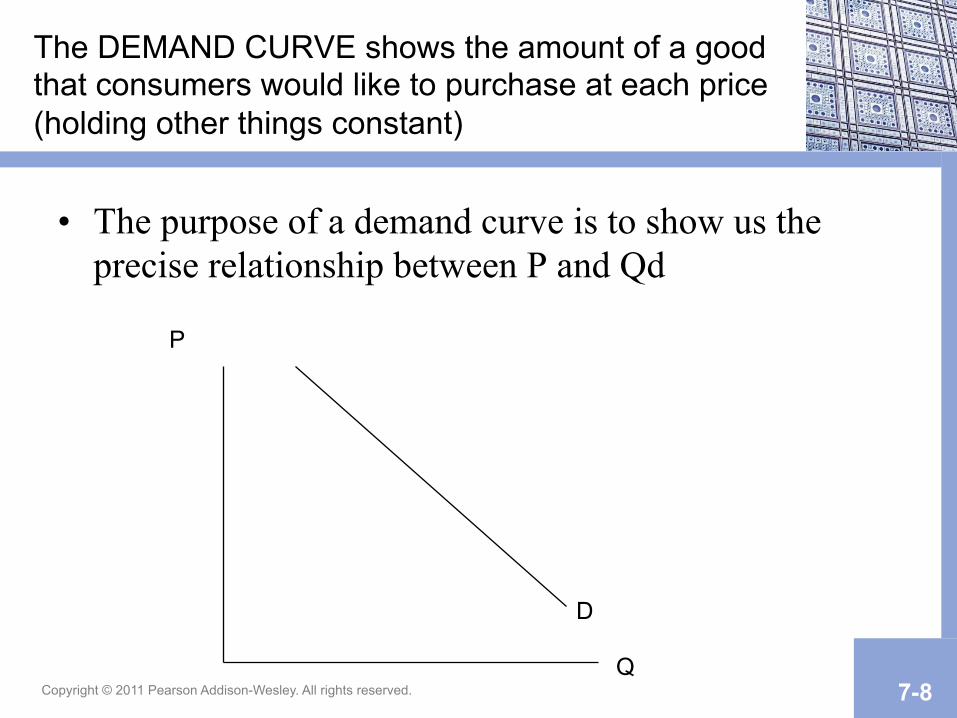
The DEMAND CURVE shows the amount of a good that consumers would like to purchase at each price (holding other things constant)

•  The purpose of a demand curve is to show us the precise relationship between P and Qd

D

P

Q


•  Other factors besides price affect the LOCATION of the Demand curve (way to the right or way to the left)

•  These factors are assumed constant for a particular demand curve.

•  When they change, you must draw an entirely new demand curve.

Determinants of Demand


Warning: you must carefully distinguish between a CHANGE IN DEMAND – a shift in the demand curve – as opposed to a movement along a demand curve, which is called a CHANGE IN QUANTITY DEMANDED

A Note of Caution


•  1. INCOME •  Normal Goods: �Income � �D

–  Example: more money � buy more beer, more CDs, etc.

•  Inferior Goods: �Income � �D –  Example: macaroni & cheese, cheap beer

Determinants of Demand: (Factors that shift the demand curve to a new location)


•  1. INCOME •  Normal Goods: �Income � �D

–  Example: more money � buy more beer, more CDs, etc.

•  Inferior Goods: �Income � �D –  Example: macaroni & cheese, cheap beer

Determinants of Demand:

P

Q

D1 D2

The effect of an increase in income on the demand for a normal good


2. TASTES & PREFERENCES: Fads & advertising influence the location and slope of the demand curve

P

Q

D D2

An effective advertising campaign can:

(1)  increase the demand for a product, shifting it to the right, and,

(2) make consumers more loyal and less likely to buy a substitute, which makes the demand curve steeper.


3. EXPECTATIONS OF FUTURE PRICES

•  If consumers expect a price increase in the future, they will buy now

•  If they expect a price decrease in the future, they will wait to purchase an item


4. PRICES OF RELATED GOODS

•  SUBSTITUTES: goods that can be used interchangeably

•  COMPLEMENTS: two goods consumed together


5. NUMBER OF CONSUMERS (Demanders)

•  More consumers means a greater demand for a product

•  Fewer consumers means the opposite


Practice Problem #1

•  Over the last 10 years, DVD players have gone from costing over $1000 to being as inexpensive as VCRs. Analyze the effects of the fall in the price of DVD players on the demand curve in the following markets: –  1. The DVD player market –  2. The VCR market –  3. The DVD disc market


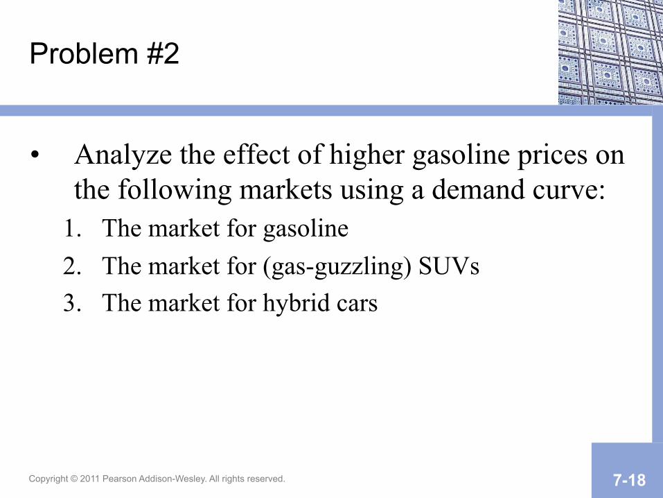
Problem #2

•  Analyze the effect of higher gasoline prices on the following markets using a demand curve:

1.  The market for gasoline 2.  The market for (gas-guzzling) SUVs 3.  The market for hybrid cars


Supply

•  Quantity Supplied: – The amount of a good or service that an economic

actor will offer for sale at a particular price


Assumptions behind the supply curve

1.  Capitalist system with privately owned firms 2. Firms maximize profits, in deciding a) what to

produce, b) how much to produce, c) how to produce

–  Occasionally some firms don't maximize profits: •  Many CEOs want to maximize their prestige, size of the

corporation, hence the use of stock options –  But most firms do maximize profits.


Supply Assumptions (Continued)

3.No 1 seller can influence the market (atomistic competition) – We'll look at non-competitive markets, where firms

can control prices, later 4. Capital &Technology are fixed in the SHORT

RUN – Short run: can't build new plants or develop new

technology – So firms cannot produce beyond their current

capacity.


1. Scarcity of resources: –  more production → more demand for resources, higher cost

of production (increasing opportunity cost) 2. Firms must be offered a higher price to induce them

to produce more than they are already producing •  LAW OF SUPPLY: Price and Quantity are directly

related: –  �P � �Quantity Supplied

Why the Supply Curve slopes upward


•  Each firm has its own supply curve •  We can also have supply curves for the entire

market for a product –  e.g., the supply of cars, the supply of beer, etc. – Market supply curve = � of individual supply

curves

Supply Curve: shows the amount firms will offer for sale at each P


Quantity

Price S

P1

P2

QS1 QS2

A typical Supply Curve:


A Change in Price causes a change in the Quantity Supplied

•  i.e., a change in prices causes a movement along the supply curve.

Quantity

Price S

P1

P2

QS1 QS2


Determinants of Supply: determine the location of S curve

•  (i.e., cause SHIFTS in S) •  1. Technology: better technology reduces costs,

shifts S down and to the right (firms can now produce more goods at a lower price)

•  Example: Computers get cheaper each year, WHY?


•  When the factors of production cost less, firms can produce more goods for the same price �S

•  Example: Lower health care costs from HMOs � lower costs of production for firms, �S

•  Example: Higher advertising expenditures would increase costs, decrease S (producers would charge a higher P for same Q).

–  Hopefully, the increase in D would offset the decrease in S.

2. Resource/Input Prices:


•  The more suppliers or competitors, the more the market supply and the lower the market price

•  In 1980s, Apple Macs cost $3000, including a $1500 profit on each computer!

•  Today, Mac makes about $150 profit per computer.

3. Number of Producers:


•  Dairy/Wheat Farmer: Wheat production depends on the Price of Milk

•  Question: How would a decrease in the price of milk affect the supply of milk and the supply of wheat, given that many forms supply both milk and wheat using the same land?

•  Another example: AT&T makes more money on their telecommunications business than it does on its personal computer business. What does it make sense for them to do? Explain using supply curves.

4. Prices of Other Goods a Firm Can Produce


•  Firms produce based on what they EXPECT to sell –  It can take up to 6 months or even a year to get a product to

market and sell it, so firms produce today what they expect to sell in the future.

–  If the future looks grim, firms cut back on production BEFORE the problems occur

-Which helps to make sure that the future is grim. –  Government forecasts are invariably rosier than the actual

situation. •  Negative forecasts can actually create a negative situation if they

affect BUSINESS CONFIDENCE

5. Expectations: about future sales, prices, the economy


Problem:

•  What will happen to the supply of oil and the supply of automobiles (car plants use energy generated by burning oil) when the price of oil increases?


EQUILIBRIUM: where QS = QD, which determines equilibrium P (Pe) and Q (Qe)

FIGURE 7.3 Market and Equilibrium Price

Pe

Qe


FIGURE 7.4 Surplus Eliminated by Price Decreases


Producers respond to a surplus by 1) lowering prices & 2) decreasing quantity supplied

•  Consumers will buy more as the price falls while firms produce less

•  Continues until Qs=Qd and we reach equilibrium


FIGURE 7.5 Shortage Eliminated by Price Increases


Suppliers will respond to a shortage in two ways

•  1) �P, and •  2) �QS. •  �P will

cause Qd to fall until we eventually reach equilibrium


Markets stay in Equilibrium unless something disturbs them:

•  Change in Demand •  Change in Supply •  Government regulations that affect S & D

– Price Floors and Price Ceilings – Excise Taxes and Per-Unit Subsidies


Supply and Demand examples

•  Effect of Federal Safety Legislation on the US Car Market – Federal Safety Legislation on air bags, side impact,

etc. → higher costs of production of about $1500 per car

– How would this affect the car market?


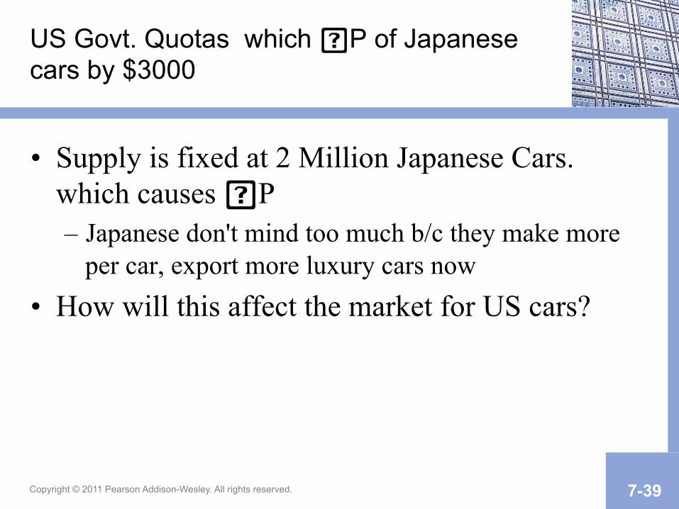
US Govt. Quotas which �P of Japanese cars by $3000

•  Supply is fixed at 2 Million Japanese Cars. which causes �P –  Japanese don't mind too much b/c they make more

per car, export more luxury cars now •  How will this affect the market for US cars?


Additional problems:

•  What effect would devaluing the dollar have on the US car market? – Each dollar buys less foreign currency (and less

foreign goods) than it used to •  What effect would Higher Gasoline Prices have

on the US car market, and the market for smaller, imported cars?


Another Problem

•  What will happen to the market for CDs when the price of DVD audio discs increases (DVD audio discs can be played in DVD players so the music can be heard in 5 speaker surround sound)?

Q (1000s)

S P

D

Compact Discs

90

$15

D2

Consumers will buy fewer DVD audio discs and more CDs.


Another Problem

•  An economic boom causes wages for workers to increase, so CD consumers have more money but CD producers have to pay more to workers. What will happen to the CD market?

Wages increase, which increases consumers’ incomes. But costs increase, causing the supply curve to shift up and to the left. The result is higher prices, but quantity remains about the same.

Q (1000s)

S P

D

Compact Discs

90

$15

D2

S’


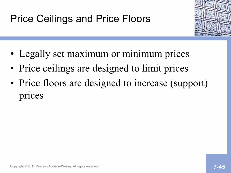
Price Ceilings and Price Floors

•  Legally set maximum or minimum prices •  Price ceilings are designed to limit prices •  Price floors are designed to increase (support)

prices


FIGURE 7.12 The Market for Gasoline with a Price Ceiling


Price Ceiling: Legally Set Maximum Price

•  Businesses cannot raise price above the ceiling – So the price ceiling must be set BELOW the

equilibrium price to be effective – With a Price Ceiling equal to or above equilibrium

price, businesses would just charge the market price (S=D)


Example: Rent Control in NYC after WWII: city govt. tries to make it affordable to live in the city, puts a maximum value on rent (a rent ceiling)

Q(MillionsofApts.)

Rent/monthS

D

1500

800

1 1.50.5

PCeiling

l

l l

Price Ceiling results in a shortage of apartments. (Qd=1.5, Qs=0.5) This results in NON-PRICE RATIONING (the invisible hand of the market tries to increase prices in other ways)


Non-Price Rationing with Rent Control

•  Long Waits for rent controlled apts. •  As rent decreases, Q of apts. decreases

–  Owners convert buildings into condos, offices –  FEWER people can find apts. in the city (the opposite of

the city council's intentions) •  Black market (side payments, such as the non-

refundable $10,000 key deposit). •  Poor maintenance and services (if people don't like

conditions, plenty of others would take the apts.) •  The 'invisible hand' of the market circumvents the

best intentions of the city council


Rent Controls in U.S. Cities Today

•  Soft rent controls – Guarantee landlords a "fair return" on their

properties and require that owners maintain their buildings.

– Allow landlords to pass along maintenance costs, improvement costs, making building upkeep quite lucrative.

– New buildings are exempt from rent controls (so there is no disincentive to building)


Price floor (support): legally set minimum price

•  Suppliers cannot charge below the price set by the govt.

•  Must be set ABOVE the mkt. price to be effective.


Example: Price floor on corn

S

D

Q (M of Tons)

P

2

2.50 P Floor

9 10 8

l

l

l

Corn Mkt. •  Govt. sets price at $2.50. •  This causes a surplus of 2 Million

tons of corn. •  The govt. MUST by this surplus,

otherwise the P floor will be ineffective (price will fall back to equilibrium).

•  This costs the govt. 2M * $2.50 = $5 Million to purchase surplus corn.

•  The govt. can then use the surplus for school lunches, foreign aid, military.

•  But the surplus corn does have storage & transport costs too.


Elasticity: measures how responsive Q is to changes in P

•  Related to the slope of the D or S curve •  Price Elasticity of Demand = ed

–  ed = (% Δ in quantity demanded) (% Δ in price)

–  ed =(ΔQ/Q1)/(ΔP/P1) •  There are five possible values for price elasticity

of demand –  Perfectly inelastic and inelastic (Q changes very little) –  Unit Elastic –  Perfectly Elastic and Elastic (Q changes a lot)


Computing ed

D

Q

P

A

B

4

3

10 12

l

l

ΔQ=2 ΔP=-1 Q1=10 P1=4 ed = (2/10)/(-1/4)=-4/5 Inelastic: percentage change in quantity was less than the percentage change in price


Perfectly Inelastic: |ed| = 0

•  % change in quantity must be 0 –  No matter how high the price goes,

people buy the same amount. –  The demand curve is vertical.

•  Example: Kidney dialysis, air & water (if scarce)

•  If S falls enough, Air will start to have a Price

•  The idea that we would have to pay for water once seemed absurd, but once the S of drinkable water declines, water has a Price

D

S

Q

P Air


Inelastic: 0 < |ed| < 1

•  % change in quantity demanded < % change in price. –  Large increase in price only lead s to a

small decrease in quantity demanded. –  Inelastic demand curves tend to be

steep •  Necessities like gas and food usually

have inelastic demand curves. •  Expensive new technology in health

care increased costs (S curve shifts up). –  Very few people decrease demand for

hospital care, although the duration of visits decreases.

•  Note: ↑P causes ↑Total Revenue for the firm because P↑ more than Q � –  Total Revenue = P * Q –  P2*Q2 > P1 * Q1

Q

P

D

S1

S2

P1

P2

Q1Q2

Hospital Visits


Unit Elastic: |ed| = 1

•  % change in quantity demanded = % change in price

•  In between steep and flat D curves •  Question: If the firm increases price by 10%,

what will happen to quantity demanded and total revenue (price times quantity)?


Elastic: |ed| > 1

•  % change in quantity demanded > % change in price.

–  A small change in price results in a large change in quantity demanded.

–  Elastic demand curves tend to be flat. –  Goods which have many substitutes, are

expensive, and are not necessities tend to have elastic demand curves.

•  When France wouldn't agree to cut agricultural subsidies, we threatened to put a 100% tariff on white wine. France backed down because this tariff would lead to a massive D (people would buy California wines instead)

•  NOTE: ↑P => � TR : P ↑ less than Q �

D

S

S+TariffP

Q

French White Wine


Perfectly Elastic: |ed| approaches infinity

•  % change in price must be 0 for ed to be infinite. The demand curve is horizontal.

•  For a farmer, they can sell their entire crop at the market price. –  If they produce twice as much

or half as much, they are too small to affect the market price.

–  For them, the D curve is a flat line at the market price.

D

Q

PS1

S2

1 Corn Farmer


Factors affecting the price elasticity of demand:

1.  Availability of Close Substitutes –  The more substitutes available, the more elastic the demand

curve for a product will be. –  Example: D for Budweiser is very elastic (many substitutes); –  but D for BEER is very inelastic

2.  Time Period n  In the short run, people have fewer options and will not change

their buying behavior very much. In the long run, changes in price have a larger impact on QD. •  Example: After ↑P of gas in the 1970s, initially, little �D

(inelastic) •  But over time, people bought smaller cars, used solar energy (more

elastic D)


Factors affecting the price elasticity of demand (cont.)

3.  Nature of Goods n  Necessities and vices tend to have inelastic

demand curves. 4.  Fraction of Income

n  Changes in the prices of big ticket items like houses and cars cause big changes in demand, while changes in the prices of inexpensive items (gum, salt) do not.


Price Elasticity of Supply es=(%ΔQs)/(%ΔP)

•  es is computed using the same formula as ed. •  The definitions for inelastic and elastic also

hold. The only real difference is that the price elasticity of supply is always greater than 0.


Factors affecting the price elasticity of supply:

•  Accessibility of Resources –  If resources are readily available then production can be

increased quickly when price increases. –  When resources are unavailable, it may take a significant

amount of time to increase the supply of a good, making the supply very inelastic in the short run.

–  Example: supply of doctors •  It takes over 8 years for a person with a college degree to become a

doctor •  So it will take at least that long for an increase in doctors' salaries to

result in an increase in the supply of doctors


Factors affecting the price elasticity of supply:

•  Time Period –  In the short run, firms have fewer options and may not be

able to increase production when prices increase. –  For example, if the price of corn increases in July, farmers

will be unable to increase the supply of corn until the next year.

•  Thus the supply of corn is very inelastic in the short run (1 year) but very elastic in the long run (2 or more years) because production can be increased easily next year.


Applications of S, D & Elasticity

•  ed for gasoline is –0.2, and OPEC reduces the supply of gasoline by 10%, from 10 million barrels per day to 9 million barrels per day. The price gas is $1.00 per gallon.

•  Solving the problem: –  10% decrease in Q will lead to a 50% increase in price –  %ΔQ/%ΔP= ed. 10%/(%ΔP)=-0.2 (%ΔP_=(.1/.2)=.5=50% –  So the price of gas increases by 50% to $1.50.

•  In the long run, we could expect more of a decline in D (more elastic D)


Baseball example

•  Major League Baseball Owners raised the price of baseball tickets by 10% a few years ago.

•  But instead of taking in more revenue, their total revenue from ticket sales (P*Q) actually DECLINED.

•  What does this tell us about the price elasticity of the demand for baseball tickets? Explain. –  ed = (%Q)/(%P)


FIGURE 7.BP.1 The Corn Market Responds to an Increase in Demand


FIGURE 7.BP.2 The Corn Market Responds to an Increase in Demand


TABLE 7.1 Demand Schedule for College Education


FIGURE 7.1 Demand Curve


TABLE 7.2 Supply Schedule for College Education


FIGURE 7.2 Supply Curve


TABLE 7.3 The Supply Schedule Combined with the Demand Schedule


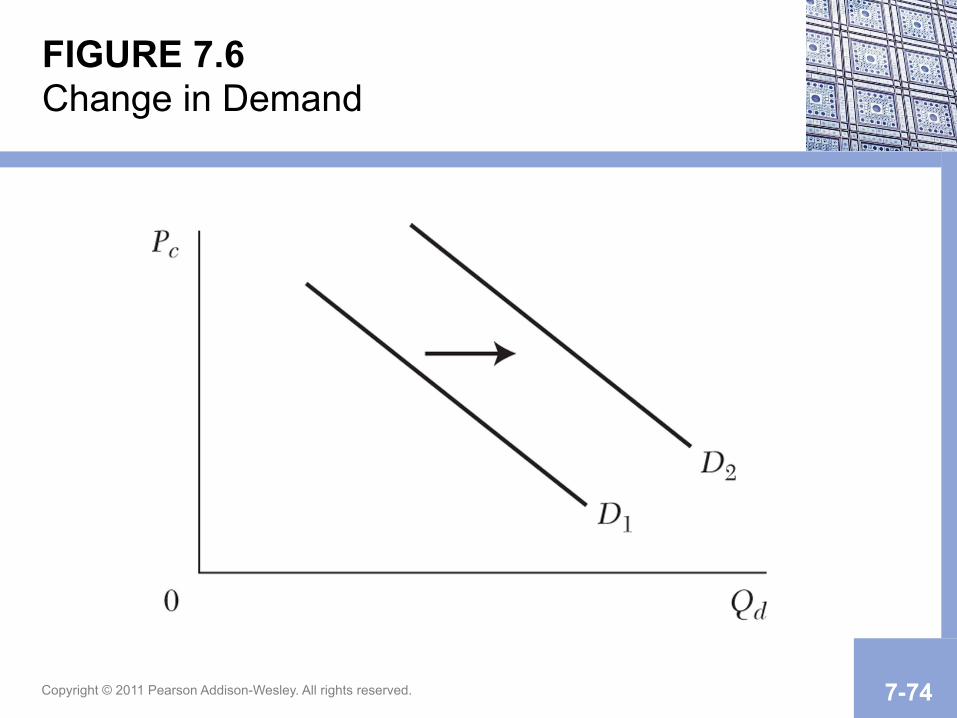
FIGURE 7.6 Change in Demand


FIGURE 7.7 Effect on Market of Change in Demand


FIGURE 7.8 Change in Supply


FIGURE 7.9 Effect on Market of Change of Supply


FIGURE 7.10 Effects of a Decrease in Demand


FIGURE 7.11 The U.S. Market for Gasoline


FIGURE 7.13 Elasticity Along a Demand Curve


TABLE 7.4 Elasticity (Ed) and Total Revenue (TR)


Documents

The Theory of Markets - · PDF file(holding other things constant) ... LOCATION of the Demand curve (way to the right or way to the left) ... causing the supply curve to shift up