The Theory of Life-Cycle Saving and Investing€¦ · 1 Introduction Life-cycle saving and investing are today a matter of intense concern to millions of people around the world

No. 07‐3

The Theory of Life‐Cycle Saving and Investing

Zvi Bodie, Jonathan Treussard, and Paul Willen

Abstract: How much should a family save for retirement and for the kids’ college education? How much insurance should they buy? How should they allocate their portfolio across different assets? What should a company choose as the default asset allocation for a mandatory retirement saving plan? We believe that the life‐cycle model developed by economists over the last fifty years provides guidance for making such decisions. The theory teaches us to view financial assets as vehicles for transferring resources across different times and outcomes over the life cycle, and that perspective allows households and planners to think about their decisions in a logical and rigorous way. This paper lays out and illustrates the basic analytical framework from the theory in nonmathematical terms, with the aim of providing guidance to financial service providers, consumers, and policymakers.

JEL Classifications: D14, D91 Zvi Bodie is the Norman and Adele Barron Professor of Management at Boston University; Jonathan Treussard is a Ph.D. candidate at Boston University; and Paul Willen is a Senior Economist and Policy Advisor at the Federal Reserve Bank of Boston. Their e‐mail addresses are [email protected], [email protected], and [email protected], respectively.

This paper, which may be revised, is available on the web site of the Federal Reserve Bank of Boston at http://www.bos.frb.org/economic/ppdp/index.htm.

The views expressed in this paper are solely those of the authors and do not reflect official positions of the Federal Reserve Bank of Boston or the Federal Reserve System.

The authors thank Phil Dybvig, Debbie Lucas, and participants at the 2006 Life‐Cycle Savings and Investment Conference hosted by Boston University and the Federal Reserve Bank of Boston for helpful comments and suggestions.

This version: May 2007

1 Introduction

Life-cycle saving and investing are today a matter of intense concern to millions of

people around the world. The most basic questions people face are:

1. How much of their income should they save for the future?

2. What risks should they insure against?

3. How should they invest what they save?

4. Should they buy or rent a house?

5. Should they get a fixed-rate mortgage or an adjustable-rate mortgage?

In this paper we argue that economic theory offers important insights and guidelines

to policymakers in government, to the financial service firms that produce life-cycle

financial products, to the advisors who make recommendations to their clients con-

cerning which products to buy, to educators who are trying to help the public make

informed choices, and ultimately to consumers who are trying to answer these ques-

tions.

The literature related to these decisions is vast and complex, and we will not

attempt to survey or summarize all of it in this paper. Instead, we lay out the

basic analytical framework using a few relatively uncomplicated models, and focus

on several key concepts. This analytical framework could serve as a valuable guide

to financial services firms in helping them to develop and explain products in terms

that are understandable to the layman.

The need for sensible financial planning advice has become particularly acute in

recent years. In the past, households relied on institutions such as pension plans spon-

sored by employers and/or labor unions, social insurance programs run by govern-

ments, and support from family or community to make financial planning decisions.

But over time institutional shifts have forced households to take greater responsibility

for their finances. Change is particularly noticeable in industrialized countries, such

as the United States, the United Kingdom, Australia, Western Europe, and Japan,

where the rapid aging of the population reflects both that people are living longer

and that they are having many fewer children. In these economies, people find they

can rely less on family and government support than in the past and must, instead,

turn to financial markets and related institutions by saving and investing for their

own retirement. Even in emerging markets, new demographic and economic realities

have prompted the beginning of widespread retirement system reforms, as seen in the

1

pension reform movements of Latin America, Eastern Europe, and, more recently,

Asia. In response to global population aging and financial deregulation, governments

and financial firms are seeking to create new institutions and services that will pro-

vide the desired protection against the financial consequences of old age, illness, and

disability and will insulate people against both inflation and asset-price fluctuations.

New opportunities are to be expected for older persons to continue employment, per-

haps on a part-time basis, and to convert their assets, particularly housing wealth,

into spendable income. For better or for worse, these developments mean that peo-

ple are being given more individual choice over their own asset accumulation and

drawdown processes. As new financial instruments transfer more responsibility and

choice to workers and retirees, the challenge is to frame risk-reward trade-offs and

cast financial decision-making in a format that ordinary people can understand and

implement.

Our framework is presented conceptually, avoiding mathematical equations. In

Section 2, we introduce the life-cycle model of consumption choice and portfolio se-

lection. We emphasize the central role of consumption in life-cycle planning. We

also highlight the use of financial assets as a means to transfer consumption from

points in an individual’s life cycle when consumption is of relatively low value to

points when consumption is relatively more valuable. Section 3 highlights five con-

cepts from the life-cycle model that are directly relevant to the practice of life-cycle

planning. These are (1) the notion of a lifetime budget constraint (Section 3.1), (2)

the relevance of contingent claims in life-cycle planning (Section 3.2), (3) the trade-off

imposed by varying costs of consumption over one’s lifetime (Section 3.3), (4) the role

of risky assets (Section 3.4), and (5) asset allocation over the life cycle (Section 3.5).

In Section 4, we recognize the complexity of life-cycle planning and the relevance of

financial frictions at the individual level, and, accordingly, we argue that it is the role

of specialized firms to engineer and deliver life-cycle products that meet the needs

of households. In Section 5, we illustrate the basic points of the paper by looking

at a real-world life-cycle financial planning decision: buying a house and getting a

mortgage. Section 6 concludes.

2

2 The theory of life-cycle portfolio and consump-

tion choice: An overview

The starting point for analysis of life-cycle portfolio choice is a model of the evolution

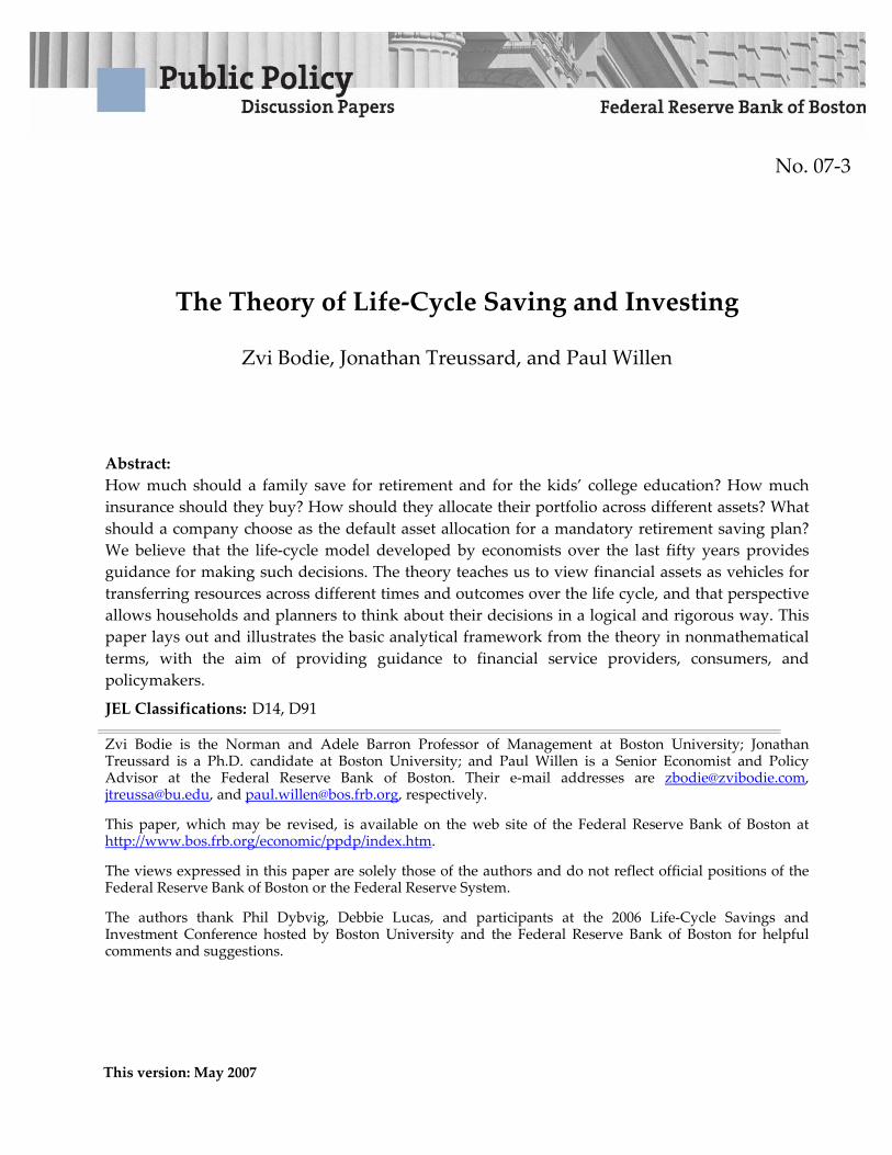
of an investor, which we can think of as an event tree.1 Figure 1 illustrates an

event tree for a fictional investor who lives for three periods: youth, prime earning

years, and retirement. In addition to aging, events occur that affect the investor. In

period 2 he earns either high or low income, and in period 3 he enjoys either good

or poor health. Figure 1 shows income and, in retirement, expenses associated with

the various outcomes. We assume that our investor earns no income in retirement

and faces no health expenses before retirement. A financial plan, in this context,

tells an investor how much to save or borrow and how to invest any savings, not just

today (in period 1) but in the future (period 2), and how much he should withdraw

in retirement (period 3). That plan may also depend on contingencies: along the

high-income path, our investor may want to save more; along a path of poor health,

our investor may want to withdraw less to prepare for high bills.

Let us suppose, for simplicity, that the only investment opportunity is to save or

borrow at 0 percent interest. The lines labeled “advice” in Figure 1 reflect a simple

proposed financial plan: save $10,000 a year when young, save $20,000 a year during

prime earning years, and withdraw $50,000 a year in retirement. It is easy to verify

that this plan works (for the age ranges shown in Figure 1): savings at retirement

equal $750,000, which, divided up over the remaining 15 years, allows withdrawals of

$50,000 a year.

How good is this proposal? Standard approaches to financial planning would focus

on whether the investor could afford to save enough or whether the $50,000 would

be enough to cover costs and desired consumption in retirement. What does the life-

cycle theory say about this proposal? We distill three principles from the life-cycle

approach:

Principle 1: Focus not on the financial plan itself but rather on the consumption

profile that it implies. In this example, we can easily calculate consumption (shown

in Figure 1), as it equals income less savings during working years, and withdrawals

less health expenses in retirement.2

Principle 2: View financial assets as vehicles for moving consumption from one

location in the life cycle to another. Suppose, for example, that our investor wanted to

1In finance, the event tree has become a workhorse tool; it is employed, most importantly, in the

Cox, Ross, and Rubinstein (1979) binomial model.2This insight goes back to Fisher (1930) and Modigliani and Brumberg (1954, 1979).

3

increase consumption in youth. By reducing saving in youth and leaving the amount

saved unchanged in prime earning years, our investor can transfer consumption from

retirement to youth. By reducing saving in youth and raising saving in middle age,

our investor can transfer consumption from prime earning years to youth.3

Principle 3: A dollar is more valuable to an investor in situations where con-

sumption is low than in situations where consumption is high. In Figure 1, for

example, the life-cycle model says that if we offer to give a dollar to our investor but

stipulate that he must choose when he wants it, our investor will want the money in

youth, when his consumption is lowest. The law of diminishing returns is at work

here: an additional dollar is much more valuable to a recent college graduate than to

a middle-aged executive.

So, what does the life-cycle model tell us about the advice in Figure 1? Looking

at the implied consumption over the life cycle, we notice huge variations. According

to our third principle above, a dollar is much more valuable when consumption is low

than when it is high. Thus, we can improve on this plan by trying to move consump-

tion from situations with high consumption to situations with low consumption. For

example:

• Consumption in youth ($20,000) is much lower (and thus more valuable) than

it is on average in prime earning years ($55,000), assuming that the high- and

low-income paths are equally likely. By saving less in youth and more in prime

earning years, our investor could transfer consumption from a low-value situa-

tion to a high-value situation and make himself better off.

• Consumption in situations HG and HB ($40,000 on average) is much lower (and

thus more valuable) than in situation H ($80,000), again assuming equally likely

outcomes. By saving more in situation H , our investor could transfer consump-

tion from low-value situations to high-value situations and make himself better

off.

• Consumption in situations LG and LB ($40,000 on average) is higher (and thus

less valuable) than in situation L ($30,000). By saving less in situation L, our

investor could transfer consumption from a low-value situation to a high-value

situation and make himself better off.

3Moving consumption over the life cycle is at the heart of life-cycle planning. As Irving Fisher put

it, the intent of life-cycle planning theory is to “modify [the income stream received by an individual]

by exchange so as to convert it into that particular form most wanted by [the individual]” (Fisher

1930, Chapter 6).

4

Now, suppose we introduce health insurance. Health insurers offer a contract that

says that for every dollar invested, the investor receives two dollars if his health is

poor in retirement. Suppose he borrows a dollar in prime earning years and invests in

health insurance: What happens? His consumption in prime earning years remains

the same, but in retirement it falls by one dollar when his health is good (because he

has to repay the loan), and increases by one dollar when his health is poor (because

he receives two dollars for having poor health less the loan repayment of one dollar).

Thus, health insurance transfers consumption resources from situations where one’s

health is good to situations where one’s health is poor. For example, in Figure 1

consumption is higher (and thus less valuable) in good health situations than in bad,

so our investor can make himself better off by buying insurance.

3 Five key concepts from the life-cycle model

3.1 Insight 1: The lifetime budget constraint

One of the great early insights in financial planning follows directly from Principle

2 above. This insight is that under certain conditions, household consumption over

the life cycle depends entirely on the present discounted value of lifetime income

and not on the evolution of income itself. More specifically, suppose two investors

each have some financial wealth and also expect some stream of labor income over

their remaining working lives.4 Calculate the discounted present value of their future

income, which we call “human wealth,” and add it to their savings and call the sum

“total wealth.” According to the life-cycle model, under certain conditions, if two

investors have the same total wealth, then their consumption decisions over the life

cycle will be the same, regardless of the shape of their actual income profiles.

To understand why we can ignore the profile of income across dates and random

outcomes, return to Principle 2 from Section 2, which says that we can use financial

assets to transfer consumption from one situation to another. A loan is a financial

asset that allows one to increase consumption today in exchange for reducing con-

sumption by the amount of the loan plus interest at a future date. What is the

maximum amount an investor can consume today? It is his current savings plus the

maximum amount he can borrow. What is the maximum amount he can borrow?

4The lifetime budget constraint is present in Fisher (1930), Modigliani and Brumberg (1954), and

Modigliani (1986). This concept of a lifetime budget constraint has been generalized and successfully

applied to life-cycle planning under uncertainty, starting most notably with Cox and Huang (1989)

and has been central to the development of finance theory over the past decade or so.

5

It is the present discounted value of his future labor income.5 Thus, total wealth,

as defined in the previous paragraph, measures the maximum amount an investor

can transfer to the present. Now that our investor has transferred everything to the

present, he can decide when to spend it, and, using the same technique, he can trans-

fer his wealth to the situations when he wants to consume. It is important to stress

that the idea of transferring all lifetime income to the present is purely a hypothetical

construct used as a way to measure lifetime resources with a single metric.

The importance of the lifetime budget constraint is that it shows that financial

wealth is only one part of an investor’s wealth. Total wealth equals financial wealth

plus human wealth. For most households, human wealth dwarfs financial wealth.

Table 1 shows the ratio of human wealth to income, measured using real-world data

for various subgroups of the population. To see the importance of human wealth,

consider a 35-year-old college graduate earning $100,000 and holding $400,000 in

financial wealth. Consider also an heir who has $3 million in financial wealth and

plans to remain out of the labor force his entire life. One might think that these two

investors have nothing in common, but according to a simple version of the life-cycle

model, they should, in fact, consume exactly the same amounts. Note that, according

to Table 1, the college graduate’s human wealth is equal to 25.9 times his current

income, or, in this case, $2.59 million; adding financial wealth of $400,000 to this

amount yields total wealth of $2.99 million, almost exactly the same as that of the

heir.

We can also incorporate future expenses into the lifetime budget constraint. For

example, suppose an investor knows that he will send two kids to college at given

dates in the future. If we know how much that education will cost, we can simply

subtract the present value of future education costs from current total wealth, just

as we added the net present value of future income.6

3.2 Insight 2: The importance of constructing “contingent

claims”

In Section 3.1 we argued that investors can use financial assets to transform their

income and expense streams into the equivalent of financial wealth, but we were not

specific as to how they could accomplish this. Now we focus on how investors can

actually effect these transformations. First, if future income and expenses are certain,

5Plus claims on future assets, although we abstract from these in the model and analysis presented

here.6See CollegeSure savings funds for an example of financial technology designed specifically to

address this need.

6

then investors can transform them into additions and subtractions from current wealth

by simply borrowing and/or saving the appropriate amounts. For example, if an

investor knows that he will earn $100,000 five years from now and if the interest rate

is fixed at 5 percent, he can raise his current liquid financial wealth by borrowing as

much as $78,350 and paying back the money (plus interest) from future earnings.

But in practice, things are not so easy. The main problem with calculating the

lifetime budget constraint is the existence of random outcomes. To see why random

outcomes are a problem, return to Figure 1. Following the logic above, our investor

can convert his future labor income into current financial wealth by borrowing. But

how much should he borrow? Along the “high-income” path, he earns $100,000 a

year. So, if we assume a zero interest rate, he could borrow $100,000 today and pay

it back at, say, age 45. But suppose he does not achieve the “high-income” outcome,

but instead earns “low income.” Then, at age 45, his income will not be sufficient

to pay off the loan. Another alternative would be to borrow $75,000, the average of

his two income draws, but he would still have insufficient funds in the low-income

scenario.

What if financial markets offered a security that pays one dollar only if our investor

draws the low-income outcome and another security that pays one dollar only if our

investor draws the high-income outcome? Then, our investor could convert his future

income along the low-income path into current income by shorting $50,000 dollars

of the low-income asset and, similarly, he could convert his income along the high-

income path using the high-income asset. We call these assets that pay off contingent

on some future event “contingent claims.”7

If contingent claims are so useful, one might ask why we don’t observe them. The

answer is that we do, although they rarely appear in the form described. In Section

2, we described health insurance, a contract that offers to pay an investor’s medical

bills in exchange for a payment today. Health insurance is not a contingent claim

per se, as it pays in both outcomes, but it is easy to construct a contingent claim

using the health insurance contract and the riskless bond. For example, if an investor

wants a claim contingent on the poor-health outcome, then he should borrow $5000

and buy health insurance. In the poor-health event, he will receive $1000, $15,000

less the loan repayment, and in the good-health event he will receive nothing, as the

health insurance payoff and the loan repayment will cancel each other out. Similarly,

one can construct a claim contingent on the good outcome.

Contingent claims help with another serious problem: inflation. Suppose our

7Or Arrow-Debreu securities, after the seminal work of Arrow (1953) and Debreu (1959). See

also Arrow (1971) and the recent work by Sharpe (2006).

7

investor knows for sure that he will earn $100,000, next year, but he is uncertain about

inflation. Say that inflation could either be 0 or 10 percent. Thus, our investor’s real

income next year actually does vary randomly: along one path, he receives $100,000 in

real spending power, and along the other, he receives $90,000. According to Principle

2 above, our investor will want to shift consumption from the low-inflation event to

the high-inflation event. If we create inflation-contingent claims, our investor will be

able to do just that. It is for this reason that economists have long advocated and

spearheaded the creation of inflation-indexed bonds, marketed as TIPS or Treasury

Inflation Protected Securities.8

We have now, we hope, convinced the reader of the value of contingent claims in

life-cycle financial planning. But before we go on, we should discuss the limits to the

use of contingent claims. First, contingent claims work well when both parties can

verify the event in question and neither party can affect or has better information

about the likelihood of the event’s occuring. For example, it is easy to verify the

price of General Motors stock, and, for the most part, investors who either have

better information or can affect the price are legally forbidden from trading, so we

see a large variety of claims that are contingent on the level of GM stock (futures,

options, etc.). But above, we proposed that an investor would buy claims contingent

on the level of his labor income. Since income is not always easy to verify (the investor

would have an incentive to hide some income and claim that he earned only $50,000

when he actually earned $100,000 so as to allow him to pay back only $50,000), and

since a worker has some control over how much he earns (again, our investor has

an incentive to earn less because he would then have to repay less), income-linked

contingent claims present practical problems.9 Second, creation of contingent claims

requires that we understand clearly the risks involved, and neither recordkeeping nor

econometric techniques have yet rendered measurement of these risks trivial.

3.3 Insight 3: The prices of securities matter!

In discussing contingent claims, we have shown how households can eliminate varia-

tion in consumption across different random events by transferring consumption from

outcomes with high consumption to outcomes with low consumption by buying and

8See, for instance, Fischer (1975) and Bodie (2003) on the role of inflation-protected bonds in

life-cycle plans.9These problems are related to moral hazard and the resulting borrowing constraint literature,

such as He and Pages (1993) and El Karoui and Jeanblanc-Picque (1998), who extend the study

of human capital in life-cycle planning to address the important real-world problems caused by the

limited ability of people to borrow against future income.

8

selling consumption in those different outcomes using contingent claims. But we have

said nothing thus far about the price of contingent claims.

To illustrate some of the issues with the pricing of contingent claims, we consider

an investor who faces two equally probable outcomes in the future: in outcome H

(the high-income outcome), he consumes $100,000, and in outcome L (the low-income

outcome), he consumes $50,000. Table 2 provides information for this example. To

analyze this problem we need two concepts from probability theory. First, we measure

the “expected” level of consumption, which we get by weighting different outcomes

by their respective probabilities and summing. The expected consumption of our

investor is $75,000. But many different consumption profiles yield the same expected

consumption (for example, $75,000 with certainty), and risk averse investors are not

indifferent between them. Our investor, if risk averse, would certainly prefer $75,000

with certainty. But we can go further and actually measure how much he prefers other

consumption profiles by measuring the “certainty equivalent consumption level,” the

level of certain consumption that would make him as happy as the random consump-

tion in question. For a reasonable level of risk aversion, we calculate that our investor

would be as happy with $70,710 with certainty as with $100,000 and $50,000 with

equal probability.10

Now, assume that a financial planner comes along to help him out. The financial

planner can offer the investor a set of contingent claims, one paying $1 in outcome

H and another paying $1 in outcome L. What strategy should he propose to the

investor? Starting with a baseline case where both contingent claims cost 50c, the

financial planner proposes to the investor that he short $25,000 of outcome-H income

by shorting the contingent claim and long $25,000 of outcome-L income by longing

the outcome-L contingent claim. The cost of the state-L contingent claim ($12,500)

is exactly offset by the gains from shorting the outcome-L contingent claim, meaning

that the portfolio costs nothing. What happens to consumption? The investor now

consumes $75,000 in both outcomes. Thus, this strategy shifts consumption from the

high outcome to the low outcome, just as we said financial assets were supposed to

do. And the certain equivalent level of consumption, trivially equal to the actual

level of consumption, $75,000, is much higher than the initial level. So the financial

planner provided good advice.

Now, we change the world by setting the prices of the contingent claims unequally,

at 40c for the H outcome and 60c for the L outcome. Suppose the planner provides

the same advice (called “Strategy 1” in the table). The plan still provides the same

10For a standard textbook treatment of this type of analysis, see Mas-Colell, Whinston, and Green

(1995).

9

certain level of consumption, but there is a slight problem: since the price of the

H-state consumption has fallen relative to the L-state, the revenue from the sale of

H-state consumption no longer offsets the cost of the added L-state consumption.

The investor needs to come up with $5000 now to execute the strategy. We assume

the investor does not have that money, and we confine ourselves to self-financing

strategies. The planner regroups and suggests Strategy 2, a self-financing strategy

that yields certain consumption of $70,000. By selling more of the cheap, state-H

claims and buying fewer of the expensive, state-L claims, our investor can achieve

certain consumption of $70,000 without adding any money. Has the planner earned his

money? No. Recall that certainty equivalent consumption for the initial consumption

profile exceeds $70,000.

So far, both strategies proposed by the planner have caused problems, one because

it required substantial additional funds and the other because it failed to provide

any benefit. Does this mean that financial planning cannot help this investor? No.

Strategy 3 offers a bundle of contingent claims that manages to raise the investor’s

certainty equivalent consumption without requiring additional investment. What is

unique about this plan among the ones we have considered so far is that it does not

provide a certain level of consumption.

Not all investors will respond to the asset prices the same way. Differences in risk

aversion, for example, play a big role. Risk aversion measures the willingness of an

investor to tolerate variation in consumption across random outcomes. Comparing

Strategies 2 and 3, we argued that our investor was willing to accept a substantial

increase in variation of consumption in exchange for a small increase in expected

consumption. But that follows only from the specific choice of risk aversion that we

made. A household with higher risk aversion might have opted for the sure consump-

tion. Another issue that has drawn significant attention from economists is “habits.”

Some have argued that households are particularly unwilling to tolerate reductions

in consumption. In this case, for example, suppose that our investor currently con-

sumed $70,000 a year and was unwilling to tolerate any reduction in consumption.

Then, for him, the only plausible option would be to accept the lower expected level

of consumption that accompanies the strategy of riskless consumption. To add to the

challenge of portfolio choice in this situation, we point out that the investor knows

that higher consumption may restrict his choices in the future, and thus he may

restrict consumption now so that he can take risky bets in the future.11

The above examples illustrate that the optimal plan depends on the prices of the

contingent claims. With either set of prices, it was possible to eliminate variability

11For a discussion of these issues, see Dybvig (1995).

10

from consumption. But in only one of the cases was this advisable. The difference

between the two scenarios is that, in the baseline, there was no risk premium and

thus no incentive for the investor to take on risk, whereas in the alternative, there

was a risk premium. To see the difference, calculate the returns on a riskless bond

that pays $1 in both outcomes and an equity-type security that pays $1 in state L,

and $2 in state H . In the baseline scenario, the price of this riskless bond would be

$1, making the return zero, while equity costs $1.50 and has an expected payoff of

$1.50, so it also has a return of zero. In the alternative scenario, the return on the

riskless bond is still zero, whereas the equity security has the same expected payoff of

$1.50 but now costs $1.40, meaning that it returns 7 percent more than the riskless

bond.

3.4 Insight 4: Risky assets in the life-cycle model

One of the most important insights of the life-cycle model concerns the benefits of

risky assets. In the life-cycle model, we view risky assets as a way to move money

across different outcomes at a given time, not as a way to transfer resources across

time. Let us illustrate this point with an example.

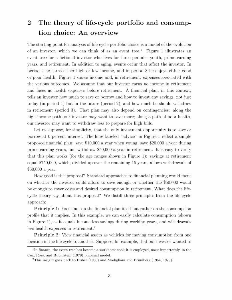
Consider the case of an investor who lives for two years, this year and a “next

year” in which there are two possible outcomes: “good times” and “bad times.” Our

investor can invest in a bond that pays 5 percent regardless of the outcome and a stock

that increases by 30 percent in good times and falls by 5 percent in bad times. Figure

2 illustrates this event tree. Standard investment advice would view the two assets as

different ways to save for the future, that is, to transfer money to the future. In the

life-cycle model, we divide the roles of these two assets. We do this by constructing

a portfolio composed of $100 of stock, financed by a $100 short position in the bond.

This portfolio costs nothing today, and, as Figure 2 shows, pays $25 in good times

and -$10 in bad times. In other words, one can use this portfolio to convert $10 in

bad times into $25 in good times (transaction 2 in the picture). To transfer money

across time, one uses the bond, which allows the investor to exchange, for example,

$100 today for $105 in both states in the future (transaction 1 in the picture).

Suppose our investor has decided to invest $100 and wants to decide whether to

invest the sum in stocks or in bonds. Our analysis shows that a $100 investment in

stock is a combination of a $100 investment in the bond and the portfolio described

above. In other words, the investor is exchanging $100 today for $105 in the future

and exchanging $10 in bad times for $25 in good times. According to our logic, we

view investing $100 in the bond as exchanging $100 today for $105 next year but

transferring nothing from bad times to good times. Thus, the difference between the

11

two investment options is not a difference about transferring resources across time—

both investments achieve that—but about transferring resources across outcomes.

The previous paragraph illustrates that the decision to invest in stocks revolves

around whether or not the investor is willing to give up $10 in bad times in exchange

for $25 in good times. If we imagine, for the purposes of discussion, that the two

outcomes are equally probable, then this seems to be an exceptionally good deal. But

we should recall that a goal of financial planning is to smooth consumption across

outcomes, so we need to know whether our investor wants to transfer income from bad

times to good times. In fact, one can imagine that our investor might want to transfer

income just the opposite way if, for example, “good times” meant employment and

“bad times” meant joblessness.

3.5 Insight 5: Asset allocation over the life cycle

One of the great early discoveries of the theory of life-cycle financial planning was an

understanding of the evolution of the optimal level of risk exposure as an investor ages.

Still-prevailing folk wisdom (and advice from some practitioners and even academics)

argues that investors should reduce the proportion of their portfolio in risky assets as

they age. This advice can be right or wrong, depending on the situation. We address

this by considering two different situations.

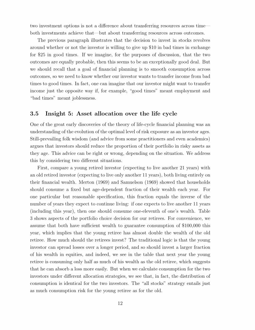
First, compare a young retired investor (expecting to live another 21 years) with

an old retired investor (expecting to live only another 11 years), both living entirely on

their financial wealth. Merton (1969) and Samuelson (1969) showed that households

should consume a fixed but age-dependent fraction of their wealth each year. For

one particular but reasonable specification, this fraction equals the inverse of the

number of years they expect to continue living: if one expects to live another 11 years

(including this year), then one should consume one-eleventh of one’s wealth. Table

3 shows aspects of the portfolio choice decision for our retirees. For convenience, we

assume that both have sufficient wealth to guarantee consumption of $100,000 this

year, which implies that the young retiree has almost double the wealth of the old

retiree. How much should the retirees invest? The traditional logic is that the young

investor can spread losses over a longer period, and so should invest a larger fraction

of his wealth in equities, and indeed, we see in the table that next year the young

retiree is consuming only half as much of his wealth as the old retiree, which suggests

that he can absorb a loss more easily. But when we calculate consumption for the two

investors under different allocation strategies, we see that, in fact, the distribution of

consumption is identical for the two investors. The “all stocks” strategy entails just

as much consumption risk for the young retiree as for the old.

12

The reason that the horizon is irrelevant here is precisely because of the nature

of consumption’s relationship with wealth. A 50 percent reduction in wealth leads to

a 50 percent reduction in consumption for both investors. It is true that the level of

wealth falls by more for the young retiree, but that level effect is exactly offset by his

consuming a smaller fraction of his wealth.

The above may suggest that the life-cycle theory has little advice to offer on asset

allocation other than to choose the right proportion at the outset. In fact, because

of the contribution of labor income, the proportion of financial wealth invested in

risky assets can vary dramatically over the life cycle. This issue was taken up by

Bodie, Merton, and Samuelson (1992), who considered life-cycle investors with risky

wages and a degree of choice with respect to the labor-leisure decision. The model’s

results indicate that the fraction of an individual’s financial wealth optimally invested

in equity should “normally” decline with age for two reasons. First, because human

capital is usually less risky than equity and the value of human capital usually declines

as a proportion of an individual’s total wealth as he ages, an individual may need to

invest a large share of his financial wealth in risky assets to achieve sufficient overall

risk exposures. Second, the flexibility that younger individuals have to alter their

labor supply allows them to invest more heavily in risky assets. The opposite result,

however, is also possible. For people with risky human capital, such as Samuelson’s

businessmen or stock analysts, the optimal path may be to start out early in life with

no stock market exposure in their investment portfolio and to increase that exposure

as they age.

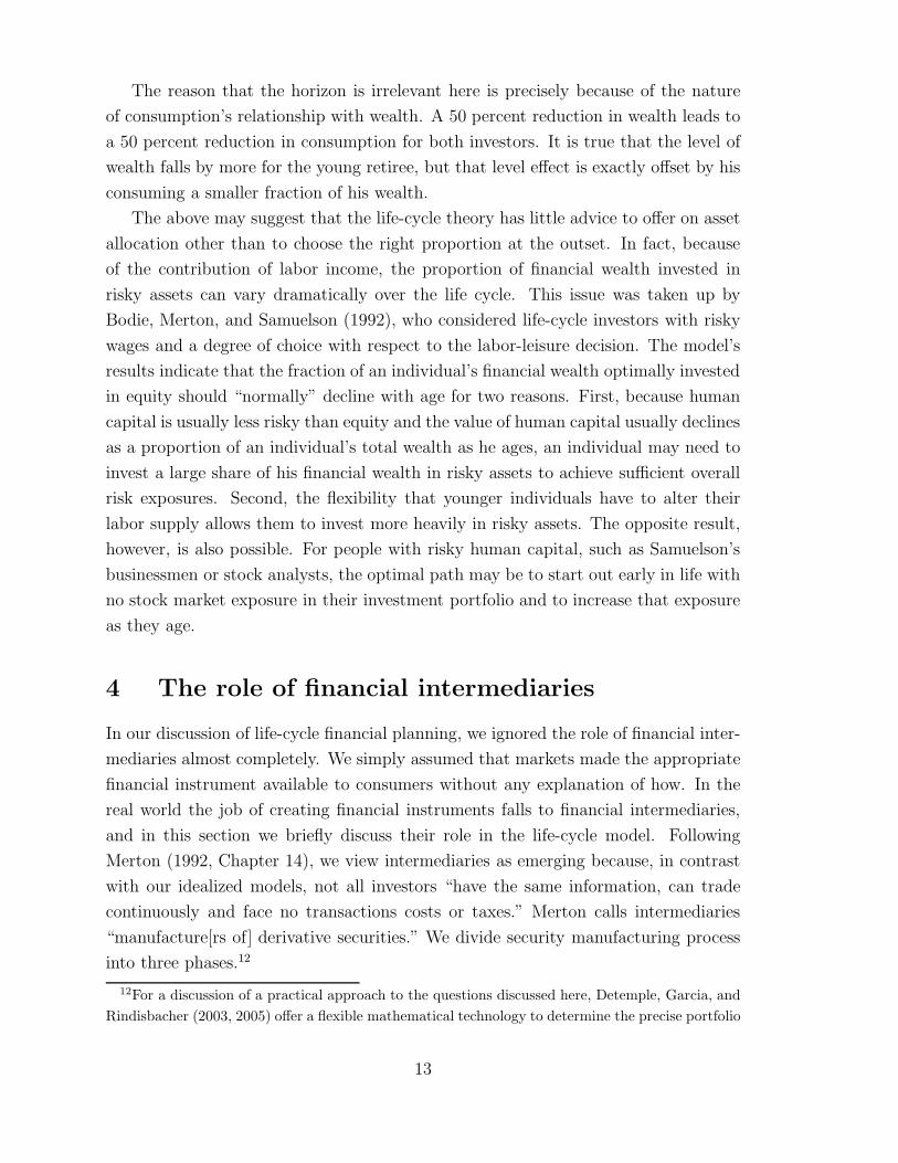
4 The role of financial intermediaries

In our discussion of life-cycle financial planning, we ignored the role of financial inter-

mediaries almost completely. We simply assumed that markets made the appropriate

financial instrument available to consumers without any explanation of how. In the

real world the job of creating financial instruments falls to financial intermediaries,

and in this section we briefly discuss their role in the life-cycle model. Following

Merton (1992, Chapter 14), we view intermediaries as emerging because, in contrast

with our idealized models, not all investors “have the same information, can trade

continuously and face no transactions costs or taxes.” Merton calls intermediaries

“manufacture[rs of] derivative securities.” We divide security manufacturing process

into three phases.12

12For a discussion of a practical approach to the questions discussed here, Detemple, Garcia, and

Rindisbacher (2003, 2005) offer a flexible mathematical technology to determine the precise portfolio

13

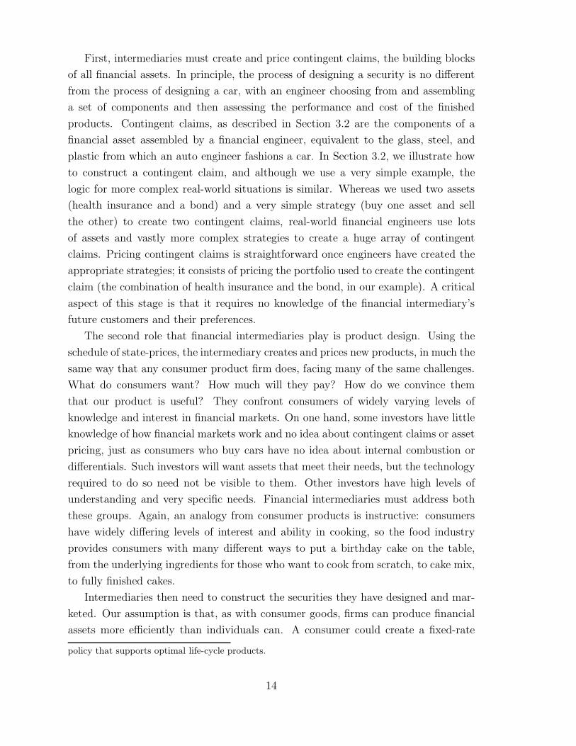
First, intermediaries must create and price contingent claims, the building blocks

of all financial assets. In principle, the process of designing a security is no different

from the process of designing a car, with an engineer choosing from and assembling

a set of components and then assessing the performance and cost of the finished

products. Contingent claims, as described in Section 3.2 are the components of a

financial asset assembled by a financial engineer, equivalent to the glass, steel, and

plastic from which an auto engineer fashions a car. In Section 3.2, we illustrate how

to construct a contingent claim, and although we use a very simple example, the

logic for more complex real-world situations is similar. Whereas we used two assets

(health insurance and a bond) and a very simple strategy (buy one asset and sell

the other) to create two contingent claims, real-world financial engineers use lots

of assets and vastly more complex strategies to create a huge array of contingent

claims. Pricing contingent claims is straightforward once engineers have created the

appropriate strategies; it consists of pricing the portfolio used to create the contingent

claim (the combination of health insurance and the bond, in our example). A critical

aspect of this stage is that it requires no knowledge of the financial intermediary’s

future customers and their preferences.

The second role that financial intermediaries play is product design. Using the

schedule of state-prices, the intermediary creates and prices new products, in much the

same way that any consumer product firm does, facing many of the same challenges.

What do consumers want? How much will they pay? How do we convince them

that our product is useful? They confront consumers of widely varying levels of

knowledge and interest in financial markets. On one hand, some investors have little

knowledge of how financial markets work and no idea about contingent claims or asset

pricing, just as consumers who buy cars have no idea about internal combustion or

differentials. Such investors will want assets that meet their needs, but the technology

required to do so need not be visible to them. Other investors have high levels of

understanding and very specific needs. Financial intermediaries must address both

these groups. Again, an analogy from consumer products is instructive: consumers

have widely differing levels of interest and ability in cooking, so the food industry

provides consumers with many different ways to put a birthday cake on the table,

from the underlying ingredients for those who want to cook from scratch, to cake mix,

to fully finished cakes.

Intermediaries then need to construct the securities they have designed and mar-

keted. Our assumption is that, as with consumer goods, firms can produce financial

assets more efficiently than individuals can. A consumer could create a fixed-rate

policy that supports optimal life-cycle products.

14

mortgage by borrowing on capital markets and hedging with a cocktail of deriva-

tives, but a financial intermediary can do the same thing at a dramatically lower

cost. Financial firms confront some different issues from consumer product firms.

Consumer product firms typically only offer only limited guarantees of the quality of

their product, but, for a financial firm, guarantees are central to the whole endeavor.

The purpose of many financial contracts, life insurance, for example, is to provide

peace of mind, so a risk that the intermediary may default on its obligations severely

reduces the value of the product.

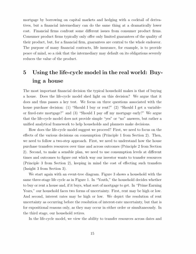
5 Using the life-cycle model in the real world: Buy-

ing a house

The most important financial decision the typical household makes is that of buying

a house. Does the life-cycle model shed light on this decision? We argue that it

does and thus passes a key test. We focus on three questions associated with the

house purchase decision: (1) “Should I buy or rent?” (2) “Should I get a variable-

or fixed-rate mortgage?” and (3) “Should I pay off my mortgage early?” We argue

that the life-cycle model does not provide simple “yes” or “no” answers, but rather a

unified analytical framework to help households and planners make decisions.

How does the life-cycle model suggest we proceed? First, we need to focus on the

effects of the various decisions on consumption (Principle 1 from Section 2). Then,

we need to follow a two-step approach. First, we need to understand how the house

purchase transfers resources over time and across outcomes (Principle 2 from Section

2). Second, to make a sensible plan, we need to use consumption levels at different

times and outcomes to figure out which way our investor wants to transfer resources

(Principle 3 from Section 2), keeping in mind the cost of effecting such transfers

(Insight 3 from Section 3).

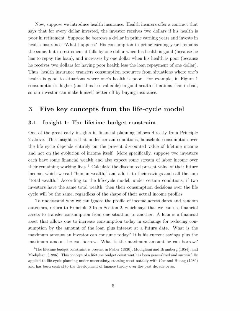
We start again with an event-tree diagram. Figure 3 shows a household with the

same three-stage life cycle as in Figure 1. In “Youth,” the household decides whether

to buy or rent a house and, if it buys, what sort of mortgage to get. In “Prime Earning

Years,” our household faces two forms of uncertainty. First, rent may be high or low.

And second, interest rates may be high or low. We depict the resolution of rent

uncertainty as occurring before the resolution of interest-rate uncertainty, but that is

for expositional reasons only, as they may occur in either order or simultaneously. In

the third stage, our household retires.

In the life-cycle model, we view the ability to transfer resources across dates and

15

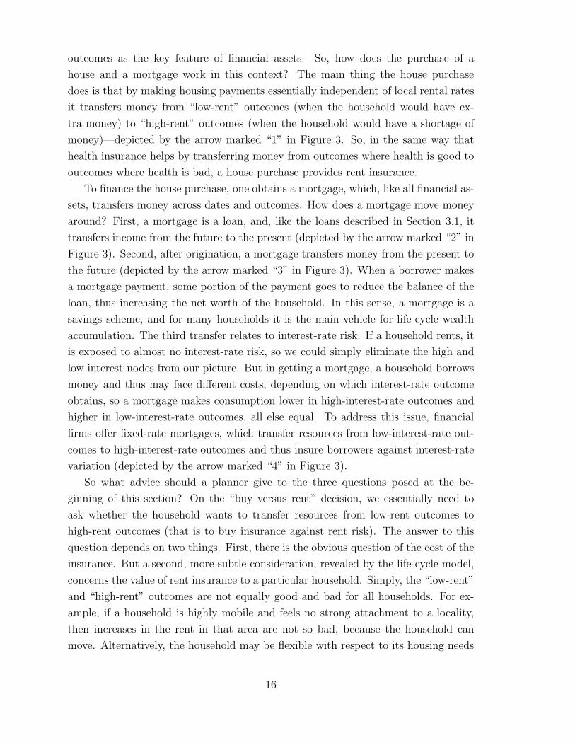
outcomes as the key feature of financial assets. So, how does the purchase of a

house and a mortgage work in this context? The main thing the house purchase

does is that by making housing payments essentially independent of local rental rates

it transfers money from “low-rent” outcomes (when the household would have ex-

tra money) to “high-rent” outcomes (when the household would have a shortage of

money)—depicted by the arrow marked “1” in Figure 3. So, in the same way that

health insurance helps by transferring money from outcomes where health is good to

outcomes where health is bad, a house purchase provides rent insurance.

To finance the house purchase, one obtains a mortgage, which, like all financial as-

sets, transfers money across dates and outcomes. How does a mortgage move money

around? First, a mortgage is a loan, and, like the loans described in Section 3.1, it

transfers income from the future to the present (depicted by the arrow marked “2” in

Figure 3). Second, after origination, a mortgage transfers money from the present to

the future (depicted by the arrow marked “3” in Figure 3). When a borrower makes

a mortgage payment, some portion of the payment goes to reduce the balance of the

loan, thus increasing the net worth of the household. In this sense, a mortgage is a

savings scheme, and for many households it is the main vehicle for life-cycle wealth

accumulation. The third transfer relates to interest-rate risk. If a household rents, it

is exposed to almost no interest-rate risk, so we could simply eliminate the high and

low interest nodes from our picture. But in getting a mortgage, a household borrows

money and thus may face different costs, depending on which interest-rate outcome

obtains, so a mortgage makes consumption lower in high-interest-rate outcomes and

higher in low-interest-rate outcomes, all else equal. To address this issue, financial

firms offer fixed-rate mortgages, which transfer resources from low-interest-rate out-

comes to high-interest-rate outcomes and thus insure borrowers against interest-rate

variation (depicted by the arrow marked “4” in Figure 3).

So what advice should a planner give to the three questions posed at the be-

ginning of this section? On the “buy versus rent” decision, we essentially need to

ask whether the household wants to transfer resources from low-rent outcomes to

high-rent outcomes (that is to buy insurance against rent risk). The answer to this

question depends on two things. First, there is the obvious question of the cost of the

insurance. But a second, more subtle consideration, revealed by the life-cycle model,

concerns the value of rent insurance to a particular household. Simply, the “low-rent”

and “high-rent” outcomes are not equally good and bad for all households. For ex-

ample, if a household is highly mobile and feels no strong attachment to a locality,

then increases in the rent in that area are not so bad, because the household can

move. Alternatively, the household may be flexible with respect to its housing needs

16

and be willing to move to a cheaper, nearby neighborhood or into a smaller house if

rent goes up.

The second question we posed concerned fixed- versus adjustable-rate mortgages.

A fixed-rate mortgage transfers resources from low- to high-interest-rate outcomes

and smooths interest rates, so the typical advisor would recommend a fixed-rate

mortgage. But the life-cycle model reminds us that we want to smooth consumption,

not interest rates, so the relevant question is whether we want to transfer resources

from low-interest-rate outcomes to high-interest-rate outcomes and the answer to that

question is, surprisingly, not obvious. High-interest-rate outcomes are often associated

with high inflation, and inflation is well known to be a borrower’s best friend as it

reduces the real value of the loan. Recall that while house values and wages generally

rise with inflation, mortgage balances are nominally fixed. This is not simply a

theoretical point: the high inflation of the late 1970s dramatically reduced the debt

burden of a generation of homeowners. By the same token, low inflation is bad news

for borrowers, so the low-interest-rate outcome could actually be very bad news for

borrowers. To sum up, if higher interest rates are associated with higher inflation,

transferring resources from low-interest-rate outcomes to high-interest-rate outcomes,

as a fixed rate mortgage does, is exactly the opposite of what the borrower wants to

do.13

Finally, we ask whether borrowers should try to pay off a mortgage. Arrow 3 in

Figure 3 points out that, through amortization, a mortgage functions as a savings

vehicle. Many people identify this as a key benefit of a mortgage, arguing that a rent

payment does not increase savings, whereas a mortgage payment does. What does

the life-cycle model tell us? The life-cycle model reminds us to focus on whether the

household actually wants to make the proposed resource transfer, that is, whether

moving money from today to retirement makes sense for a particular household. At

some point in life, it typically does, but early in the life cycle, it often does not:

household income and consumption are typically much lower than they will be in

retirement, meaning that saving will transfer resources from times when it is more

valuable to times when it is less — exactly the opposite of what households want to

do. One can see this in the data by observing that most young homeowners offset

their mortgage-related savings by borrowing, using other instruments like credit cards,

which typically charge much higher interest rates than the mortgage.

13Campbell and Cocco (2003) argued that because of the inflation benefits, adjustable-rate mort-

gages make sense for most households.

17

6 Conclusion

At the beginning of this paper, we posed a series of questions that the typical house-

hold faces in making lifetime financial plans. Now at the end, one must ask whether

we have answered any of them. The answer is no. Have we failed to deliver or are

we guilty of false advertising? We believe we aren’t. The purpose of life-cycle theory

is not to provide clear-cut answers but rather to provide a framework for individuals

and planners to figure out those answers. In fact, we view the failure to provide

simple answers as a virtue of the model: it allows planners to adjust their advice to

the enormous variations across households in income, future prospects, health, and

even tastes.

The theory described in this paper only scratches the surface of academic research

on the topic, which addresses many real-world problems that we ignored here. In par-

ticular, we made no mention of the many institutional issues that limit the portfolios

available to households. Home buyers, for example, face limits on how much they can

borrow as a function of both the value of the house they want to buy and their current

income. Investors face limits on short sales and on how much of their assets they can

use as collateral for loans. In addition, trading costs make frequent adjustment of

portfolio shares prohibitively expensive.

18

References

[1] Arrow, K. (1953), “The Role of Securities in the Optimal Allocation of Risk-

Bearing,” Econometrie; translated and reprinted in 1964, Review of Economic

Studies, 31, pp. 91–6.

[2] Arrow, K. (1971), “Insurance, Risk, and Resource Allocation,” Chapter 5 in

Essays in the Theory of Risk-Bearing, Markham Publishing Company, New York.

[3] Bodie, Z. (2003), “Thoughts on the Future: Life-Cycle Investing in Theory and

Practice,” Financial Analysts Journal, 59(1), pp. 24–29.

[4] Bodie, Z., Merton, R., and W. Samuelson (1992), “Labor Supply Flexibility and

Portfolio Choice in a Life-Cycle Model,” Journal of Economic Dynamics and

Control, 16, pp. 427–449.

[5] Campbell, J. and J. Cocco (2003), “Household Risk Management and Optimal

Mortgage Choice,” The Quarterly Journal of Economics, 118, pp. 1449–1494.

[6] Cox, J., S. Ross, and M. Rubinstein (1979), “Option Pricing: A Simplified Ap-

proach,” Journal of Financial Economics, 7, pp. 87–106.

[7] Cox, J. and C. Huang (1989), “Optimum Consumption and Portfolio Policies

When Asset Prices Follow a Diffusion Process,” Journal of Economic Theory,

49, pp. 33–83.

[8] Debreu, G. (1959), Theory of Value,Yale University Press, New Haven, CN.

[9] Detemple, J., R. Garcia, and M. Rindisbacher (2003), “A Monte Carlo Method

for Optimal Portfolios,” Journal of Finance, 58(1), pp. 401–446.

[10] Detemple, J., R. Garcia, and M. Rindisbacher (2005), “Intertemporal Asset Al-

location: A Comparison of Methods,” Journal of Banking and Finance, 29(11),

pp. 2821–2848.

[11] Dybvig, P. (1995), “Dusenberry’s Racheting of Consumption: Optimal Dynamic

Consumption and Investment Given Intolerance for any Decline in Standard of

Living,” Review of Economic Studies, 62(2), pp. 287–313.

[12] El Karoui, N. and M. Jeanblanc-Picque (1998), “Optimization of Consumption

with Labor Income,” Finance and Stochastics, 2, pp. 409–440.

19

[13] Fisher, I. (1930), The Theory of Interest, Kelley and Millman, New York,

reprinted in 1954.

[14] Fischer, S. (1975), “The Demand for Index Bonds,” Journal of Political Econ-

omy, 83(3), pp. 509–534.

[15] He, H. and H. Pages (1993), “Labor Income, Borrowing Constraints, and Equi-

librium Asset Prices,” Economic Theory, 3, pp. 663–696.

[16] Mas-Colell, A., M. Whinston, and J. Green (1995), Microeconomic Theory, Ox-

ford University Press, New York.

[17] Merton, R. (1969), “Lifetime Portfolio Selection under Uncertainty: The

Continuous-Time Case,” Review of Economics and Statistics, 51, pp. 247–257.

[18] Merton, R. (1992), Continous-Time Finance, Blackwell, Malden, MA.

[19] Modigliani, F. (1986), “Life Cycle, Individual Thrift, and the Wealth of Nations,”

American Economic Review, 76(3), pp. 297–313.

[20] Modigliani, F. and R. Brumberg (1954), “Utility Analysis and the Consumption

Function: An Interpretation of Cross-Section Data,” in K. Kurihara (ed.), Post

Keynesian Economics, Rutgers University Press, New Brunswick, NJ.

[21] Modigliani, F. and R. Brumberg (1979), “Utility Analysis and Aggregate Con-

sumption Functions: An Attempt at Integration,” in A. Abel (ed.), Collected

Papers of France Modigliani, Vol. 2, MIT Press, Cambridge, MA.

[22] Samuelson, P. (1969), “Lifetime Portfolio Selection by Dynamic Programming,”

Review of Economics and Statistics, 51, pp. 239–246.

[23] Sharpe, W. (2006), “Retirement Financial Planning: A State/Preference Ap-

proach,” Working paper.

20

Table 1: Human wealth measured as a fraction of current income. For example,

a 25-year-old college graduate has human wealth equal to 47.4 times his current

income. Source: Authors’ calculations based on data from the Panel Study of Income

Dynamics. Unless stated differently, the expected retirement age is 65.Initial Age

25 35 45 55 65

High School Graduates

Men 29.7 19.1 12.8 8.2 -

(= 718,530

24,199) (= 629,378

33,005) (= 439,494

34,301) (= 219,269

26,814) -

Women 27.9 16.6 11.9 8.6 -

(= 379,592

13,606) (= 317,191

19,159) (= 202,351

16,997) (= 101,256

11,784) -

College Graduates

Men 47.4 25.9 15.9 8.7 -

(= 1,483,412

31,297) (= 1,483,295

57,264) (= 1,212,542

76,385) (= 691,057

79,566) -

Women 32.9 20.1 13.3 7.0 -

(= 881,762

26,808) (= 792,354

39,424) (= 580,133

43,506) (= 266,430

38,064) -

Male College Graduates

Retire at 55 39.3 20.0 9.9 -

(= 1,231,486

31,297) (= 1,144,728

57,264) (= 757,535

76,385) - -

Retire at 75 51.0 28.6 18.6 12.2 7.0

(= 1,597,261

31,297) (= 1,636,299

57,264) (= 1,418,165

76,385) (= 967,398

79,566) (= 432,870

61,491)

Male, Advanced Degree Holders

51.0 28.1 16.7 9.2 -

(= 1,651,729

32,386) (= 1,709,956

60,773) (= 1,431,000

85,798) (= 866,733

94,627) -

21

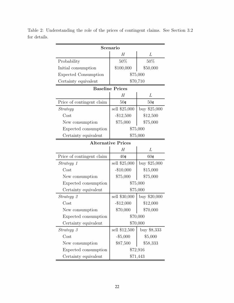
Table 2: Understanding the role of the prices of contingent claims. See Section 3.2

for details.

Scenario

H L

Probability 50% 50%

Initial consumption $100,000 $50,000

Expected Consumption $75,000

Certainty equivalent $70,710

Baseline Prices

H L

Price of contingent claim 50c 50c

Strategy sell $25,000 buy $25,000

Cost -$12,500 $12,500

New consumption $75,000 $75,000

Expected consumption $75,000


Alternative Prices

H L

Price of contingent claim 40c 60c

Strategy 1 sell $25,000 buy $25,000

Cost -$10,000 $15,000





Cost -$12,000 $12,000





Cost -$5,000 $5,000




22

Table 3: Understanding the role of age on portfolio choice in a life-cycle model. See

Section 3.5 for details.

Young Retiree Old Retiree

This year

# of years remaining in life 21 11

Consumption /wealth 1/21 1/11

Wealth $2.1m $1.1m

Consumption $100,000 $100,000

Investment $2m $1m

Next year

# of years remaining in life: 20 10

Consumption/wealth 1/20 1/10

L H L H

Bond Return 0% 0% 0% 0%

Stock Return -50% 100% -50% 100%

Strategy 1: All Bonds

Wealth $2m $2m $1m $1m

Consumption $100,000 $100,000 $100,000 $100,000

Strategy 2: All Stocks

Wealth $1m $4m $500,000 $2m

Consumption $50,000 $200,000 $50,000 $200,000

Strategy 3: 50/50

Wealth $1.5m $3m $750,000 $1.5m

Consumption $75,000 $150,000 $75,000 $150,000

23

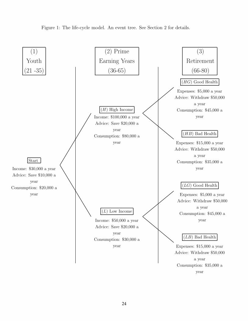
Figure 1: The life-cycle model. An event tree. See Section 2 for details.

(1)

Youth

(21 -35)

(2) Prime

Earning Years

(36-65)

(3)

Retirement

(66-80)

Start

Income: $30,000 a year

Advice: Save $10,000 a

year

Consumption: $20,000 a

year

(H) High Income



year


year

(L) Low Income



year


year

(HG) Good Health

Expenses: $5,000 a year

Advice: Withdraw $50,000

a year


year

(HB) Bad Health



a year


year

(LG) Good Health



a year


year

(LB) Bad Health



a year


year

24

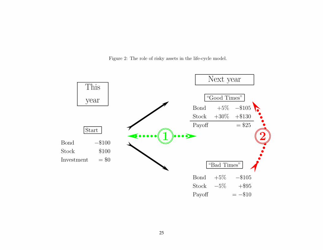
Figure 2: The role of risky assets in the life-cycle model.

This

year

Next year

Start

Bond −$100

Stock $100

Investment = $0

1 2

“Good Times”

Bond +5% −$105

Stock +30% +$130

Payoff = $25

“Bad Times”

Bond +5% −$105

Stock −5% +$95

Payoff = −$10

25

Figure 3: Analyzing the house purchase decision in a life-cycle model. See Section 5 for details.

(1)

Youth

(2) Prime

Earning Years

(3)

Retirement

Buy or rent a

house?

High Rent

Low Rent

High interest rates

Low interest rates

High interest rates

Low interest rates

Retirement12 3

4

4

26

Documents

The Theory of Life-Cycle Saving and Investing€¦ · 1 Introduction Life-cycle saving and investing are today a matter of intense concern to millions of people around the world