The Teradata Scalability Story - Spotlight Technology Teradata Scalability Story EB-3031 > 0509 > PAGE 2 OF 26 Executive Summary Scalability is a term that is widely used and often

The Teradata Scalability Story

By: Carrie Ballinger, Senior Technical Advisor, Teradata Development

Data Warehousing

http://www.teradata.com


EB-3031 > 0509 > PAGE 2 OF 26

Executive Summary

Scalability is a term that is widely used and often misunderstood. This

paper explains scalability as experienced within a data warehouse and

points to several unique characteristics of the Teradata Database that

allow linear scalability to be achieved.

Examples taken from seven different client benchmarks illustrate and

document the inherently scalable nature of the Teradata Database.

> Two different examples demonstrate scalability when the configuration

size is doubled.

> Two other examples illustrate the impact of increasing data volume,

the first by a factor of 3, the second by a factor of 4. In addition, the

second example considers scalability differences between high-priority

and lower-priority work.

> Another example focuses on scalability when the number of users, each

submitting hundreds of queries, increases from ten to 20, then to 30,

and finally to 40.

> In a more complex example, both hardware configuration and data

volume increase proportionally, from six nodes at 10TB, to 12 nodes

at 20TB.

> In the final example, a mixed-workload benchmark explores the impact

of doubling the hardware configuration, increasing query-submitting

users from 200 to 400, and growing the data volume from 1TB to

10TB, and finally, up to 20TB.

While scalability may be considered and observed in many different contexts,

including in the growing complexity of requests being presented to the

database, this paper limits its discussion of scalability to these three vari-

ables: Processing power, number of concurrent queries, and data volume.

Table of Contents

Executive Summary 2

Introduction 4

Scalability in the Data Warehouse 4

Teradata Database Characteristics that Support Linear Scalability 5

Examples of Scalability in Teradata Client Benchmarks 10

Conclusion 25



EB-3031 > 0509 > PAGE 3 OF 26

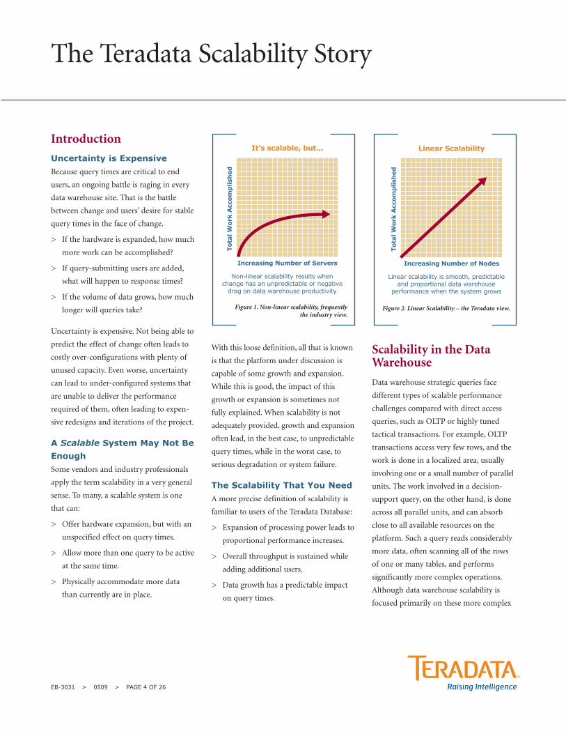
Figure 1. Non-linear scalability, frequently the industry view. 4

Figure 2. Linear Scalability – the Teradata view. 4

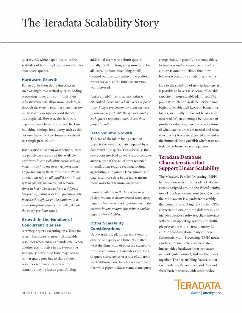
Figure 3. Many SMP nodes can be combined into a single system image. 6

Figure 4. Teradata Database's architecture. 7

Figure 5. Most aggregations are performed on each AMP locally, then across all AMPs. 7

Figure 6. BYNET merge processing eliminates the need to bring data to one node for a large final sort. 8

Figure 7. Test results when the number of nodes is doubled. 10

Figure 8. Sequential run vs. concurrent comparison, at two nodes and four nodes. 12

Figure 9. Query-per-hour rates at different concurrency levels. 14

Figure 10. Stand-alone query comparisons as data volume grows. 16

Figure 11. Average response times with data growth when different priorities are in place. 18

Figure 12. Impact on query throughput of adding background load jobs. 19

Figure 13. For small tables, data growth may not result in increased I/O demand. 21

Figure 14. Doubling the number of nodes and doubling the data volume. 22

Figure 15. A multi-dimension scalability test. 23

Table 1. Total response time (in seconds) for each of four tests, before and after the nodes were doubled. 11

Table 2. Total elapsed time (in seconds) for the 2-node tests vs. the 4-node tests. 12

Table 3. Total elapsed time (in seconds) for sequential executions vs. concurrent executions. 13

Table 4. Query rates are compared as concurrent users increase. 14

Table 5. Data volume growth by table. 16

Table 6. Query response time differences as data volume increases. 17

Table 7. Response times (in seconds) for different priority queries as data volume grows. 19

Table 8. Average response time comparisons (in seconds) afterdoubling nodes and doubling data volume. 20

Table 9. Average response time (in seconds) as nodes are doubled. 24

Table 10. Impact on average response time (in seconds) when number of users is doubled. 24

Table 11. Impact on total execution time (in seconds) as data volume increases. 25

Table 12: Average and total response times (in seconds) when both nodes and data volume double. 25

List of Figures and Tables



EB-3031 > 0509 > PAGE 4 OF 26

Introduction

Uncertainty is ExpensiveBecause query times are critical to end

users, an ongoing battle is raging in every

data warehouse site. That is the battle

between change and users’ desire for stable

query times in the face of change.

> If the hardware is expanded, how much

more work can be accomplished?

> If query-submitting users are added,

what will happen to response times?

> If the volume of data grows, how much

longer will queries take?

Uncertainty is expensive. Not being able to

predict the effect of change often leads to

costly over-configurations with plenty of

unused capacity. Even worse, uncertainty

can lead to under-configured systems that

are unable to deliver the performance

required of them, often leading to expen-

sive redesigns and iterations of the project.

A Scalable System May Not BeEnoughSome vendors and industry professionals

apply the term scalability in a very general

sense. To many, a scalable system is one

that can:

> Offer hardware expansion, but with an

unspecified effect on query times.

> Allow more than one query to be active

at the same time.

> Physically accommodate more data

than currently are in place.

With this loose definition, all that is known

is that the platform under discussion is

capable of some growth and expansion.

While this is good, the impact of this

growth or expansion is sometimes not

fully explained. When scalability is not

adequately provided, growth and expansion

often lead, in the best case, to unpredictable

query times, while in the worst case, to

serious degradation or system failure.

The Scalability That You NeedA more precise definition of scalability is

familiar to users of the Teradata Database:

> Expansion of processing power leads to

proportional performance increases.

> Overall throughput is sustained while

adding additional users.

> Data growth has a predictable impact

on query times.

Scalability in the DataWarehouse

Data warehouse strategic queries face

different types of scalable performance

challenges compared with direct access

queries, such as OLTP or highly tuned

tactical transactions. For example, OLTP

transactions access very few rows, and the

work is done in a localized area, usually

involving one or a small number of parallel

units. The work involved in a decision-

support query, on the other hand, is done

across all parallel units, and can absorb

close to all available resources on the

platform. Such a query reads considerably

more data, often scanning all of the rows

of one or many tables, and performs

significantly more complex operations.

Although data warehouse scalability is

focused primarily on these more complex

Tota

l Work

Acc

om

plis

hed

Increasing Number of Servers

Figure 1. Non-linear scalability, frequently the industry view.

Tota

l Work

Acc

om

plis

hed

Increasing Number of Nodes

Figure 2. Linear Scalability – the Teradata view.


queries, this white paper illustrates the

scalability of both simple and more complex

data access queries.

Hardware Growth For an application doing direct access,

such as single-row tactical queries, adding

processing nodes and communication

infrastructure will allow more work to get

through the system, resulting in an increase

in tactical queries-per-second that can

be completed. However, this hardware

expansion may have little or no effect on

individual timings for a query such as this

because the work it performs is localized

to a single parallel unit.

But because most data warehouse queries

are parallelized across all the available

hardware, linear scalability means adding

nodes can reduce the query response time

proportionally to the hardware growth for

queries that rely on all parallel units in the

system (double the nodes, cut response

times in half). Looked at from a different

perspective, adding nodes can proportionally

increase throughput on the platform in a

given timeframe (double the nodes, double

the query-per-hour rates).

Growth in the Number ofConcurrent QueriesA strategic query executing on a Teradata

system has access to nearly all available

resources when running standalone. When

another user is active in the system, the

first query’s execution time may increase,

as that query now has to share system

resources with another user whose

demands may be just as great. Adding

additional users who submit queries

usually results in longer response time for

all users, but how much longer will

depend on how fully utilized the platform

resources were at the time concurrency

was increased.

Linear scalability as users are added is

established if each individual query’s response

time changes proportionally to the increase

in concurrency (double the queries, double

each query’s response time), or less than

proportionally.

Data Volume Growth The size of the tables being acted on

impacts the level of activity required by a

data warehouse query. This is because the

operations involved in delivering a complex

answer, even if the set of rows returned

is small, often require reading, sorting,

aggregating, and joining large amounts of

data, and more data in the tables means

more work to determine an answer.

Linear scalability in the face of an increase

in data volume is demonstrated when query

response time increases proportionally to the

increase in data volume (the volume doubles,

response time doubles).

Other ScalabilityConsiderationsData warehouse platforms don’t tend to

execute one query at a time. No matter

what the dimension of observed scalability,

it will reveal more if it includes some level

of query concurrency or a mix of different

work. Although one benchmark example in

this white paper includes stand-alone query

comparisons, in general, a system’s ability

to function under a concurrent load is

a more favorable attribute than how it

behaves when only a single user is active.

Due to the speed-up of new technology, it

is possible to have a false sense of scalable

capacity on non-scalable platforms. The

point at which non-scalable performance

begins to exhibit itself keeps on being driven

higher, so initially it may not be as easily

observed. When entering a benchmark or

product evaluation, careful consideration

of what data volumes are needed and what

concurrency levels are expected now and in

the future will help establish whether or not

scalable performance is a requirement.

Teradata DatabaseCharacteristics thatSupport Linear Scalability

The Massively Parallel Processing (MPP)

hardware on which the Teradata Database

runs is designed around the shared nothing

model.1 Each processing unit (node) within

the MPP system is a hardware assembly

that contains several tightly coupled CPUs,

connected to one or more disk arrays, and

includes database software, client interface

software, an operating system, and multi-

ple processors with shared memory. In

an MPP configuration, many of these

Symmetric Multi-Processing (SMP) nodes

can be combined into a single-system

image with a hardware inter-processor

network (interconnect) linking the nodes

together. The key enabling feature is that

each node is self-contained and does not

share basic resources with other nodes.


EB-3031 > 0509 > PAGE 5 OF 26


These shared nothing nodes in an MPP

system are useful for growing systems

because when hardware components,

such as disk or memory, are shared

system-wide, there is an extra tax paid –

overhead to manage and coordinate the

competition for these components. This

overhead can place a limit on scalable

performance when growth occurs or stress

is placed on the system.

Because a shared nothing hardware

configuration can minimize or eliminate

the interference and overhead of resource

sharing, the balance of disk, interconnect

traffic, memory power, communication

bandwidth, and processor strength can

be maintained. And because the Teradata

Database is designed around a shared

nothing model as well, the software can

scale linearly with the hardware.

What is a Shared NothingDatabase? In a hardware configuration, it’s easy to

imagine what a shared nothing model

means: Modular blocks of processing

power are incrementally added, avoiding

overhead associated with sharing compo-

nents. Although less easy to visualize,

database software can be designed to

follow the same approach. The Teradata

Database, in particular, has been designed

to grow at all points and use a foundation

of self-contained, parallel processing units.

The Teradata Database relies on techniques

such as the ones discussed here to enable

a shared nothing model.

Teradata Database Parallelism

Parallelism is built deep into the Teradata

Database. Each parallel unit is a virtual

processor (VPROC) known as an Access

Module Processor (AMP). Anywhere

from six to 36 of these AMP VPROCs

are typically configured per node. They

eliminate dependency on specialized

physical processors, and more fully utilize

the power of the SMP node.

Rows are automatically assigned to AMPs

at the time they are inserted into the

database, based on the value of their

primary index column.2 Each AMP owns

and manages rows that are assigned to its

care, including manipulation of the data,

sorting, locking, journaling, indexing,

loading, and backup and recovery func-

tions. The Teradata Database’s shared

nothing units of parallelism set a foundation

for scalable data warehouse performance,

reducing the system-wide effort of deter-

mining how to divide up the work for

most basic functionality.

No Single Points of Control

Just as all hardware components in a shared

nothing configuration are able to grow,

all Teradata Database processing points,

interfaces, gateways, and communication

paths can increase without compromise

during growth. Additional AMPs can be

easily added to a configuration for greater

dispersal of data and decentralization of

control, with or without additional hard-

ware. The Teradata Database’s data diction-

ary rows are spread evenly across all AMPs

in the system, reducing contention for this

important resource.

In addition, each basic processing hardware

unit (node) in a Teradata system can have

one or more virtual processors known as

parsing engines (PE). These PEs support

and manage users and external connec-

tions to the system and perform query

optimization. Parsing engines can easily

increase as demand for those functions

grow, contrary to non-parallel architec-

tures where a single session-handling or


EB-3031 > 0509 > PAGE 6 OF 26

Figure 3. Many SMP nodes can be combined into a single system image.

Interconnect

SMP SMP SMP SMP

Teradata

MPP


optimization point can hold up work in a

busy system. Parsing engines perform a

function essential to maintaining scalabil-

ity: Balancing the workload across all

hardware nodes and ensuring unlimited

and even growth when communications

to the outside world need to expand.

Control over the Flow of Work from the

Bottom Up

Too much work can overwhelm the best of

databases. Some database systems control

the amount of work active in the system at

the top by using a coordinator or a single

control process. This coordinator not only

can become a bottleneck itself, but also

has a universal impact on all parts of the

system and can lead to a lag between the

freeing up of resources at the lower levels

and their immediate use.

The Teradata Database can operate near

the resource limits without exhausting any

of them by applying control over the flow

of work at the lowest possible level in the

system, the AMP. Each AMP monitors its

own utilization of critical resources, and if

any of these reach a threshold value, further

message delivery is throttled at that location,

allowing work already underway to be

completed. Each AMP has flow control

gates through which all work coming into

that AMP must pass. An AMP can close

its flow control gates temporarily when

demand for its services becomes excessive,

while other AMPs continue to accept new

work. With the control at the lowest level,

freed-up resources can be immediately put

to work, and only the currently overworked

part of the system grants itself temporary

relief, with the least possible impact on

other components.

Conservative Use of the Interconnect

Poor use of any component can lead to non-

linear scalability. The Teradata Database

relies on the Teradata BYNET® interconnect

for delivering messages, moving data,

collecting results, and coordinating work

among AMPs in the system. The BYNET is

a high-speed, multi-point, active, redundant

switching network that supports scalability

of more than 1,000 nodes in a single system.

Even though the BYNET bandwidth is

immense by most standards, care is taken

to keep the interconnect usage as low as

possible. AMP-based locking and journal-

ing keeps those activities local to one node


EB-3031 > 0509 > PAGE 7 OF 26

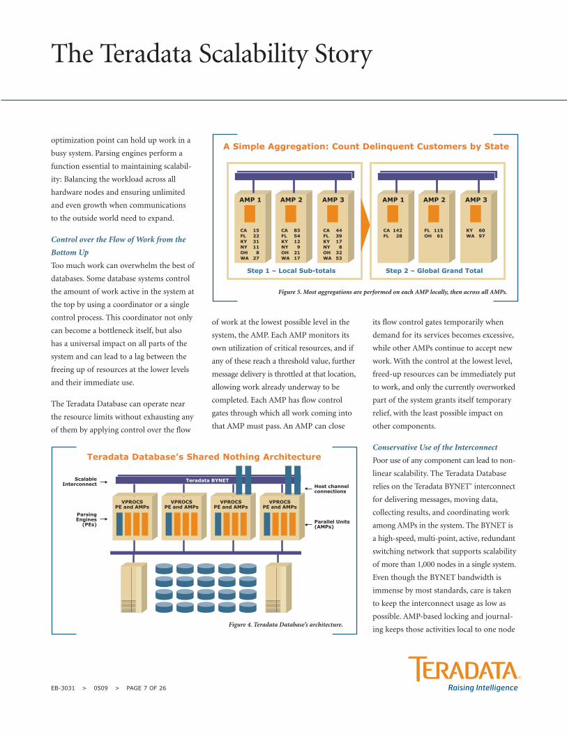
Teradata BYNET

VPROCSPE and AMPs

VPROCSPE and AMPs

VPROCSPE and AMPs

VPROCSPE and AMPs

Host channelconnections

Parallel Units(AMPs)

ScalableInterconnect

ParsingEngines

(PEs)

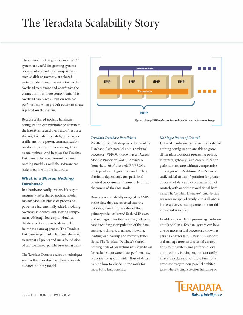
Figure 5. Most aggregations are performed on each AMP locally, then across all AMPs.

AMP 1

CA 15FL 22KY 31NY 11OH 8WA 27

AMP 2

Step 1 – Local Sub-totals


AMP 3


AMP 1

CA 142FL 28

AMP 2

Step 2 – Global Grand Total

FL 115OH 61

AMP 3

KY 60WA 97

Teradata Database’s Shared Nothing Architecture

Figure 4. Teradata Database’s architecture.

A Simple Aggregation: Count Delinquent Customers by State


without the need for outbound communi-

cations. Without the Teradata Database’s

concept of localized management, these

types of housekeeping tasks would, out of

necessity, involve an extra layer of system-

wide communication, messaging, and data

movement – overhead that impacts the

interconnect and CPU usage as well.

The optimizer tries to conserve BYNET

traffic when query plans are developed,

hence avoiding joins, whenever possible,

that redistribute large amounts of data

from one node to another. When it makes

sense, aggregations are performed on the

smallest possible set of sub-totals within the

local AMP before a grand total is performed.

When BYNET communication is required,

the Teradata system conserves this resource

by selecting, projecting, and at times, even

aggregating data from relational tables as

early in the query plan as possible. This

keeps temporary spool files that may need

to pass across the interconnect as small as

possible. Sophisticated buffering techniques

and column-based compression ensure

that data that must cross the network are

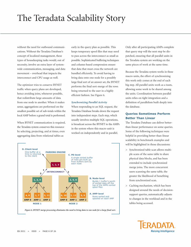
bundled efficiently. To avoid having to

bring data onto one node for a possibly

large final sort of an answer set, the BYNET

performs the final sort-merge of the rows

being returned to the user in a highly

efficient fashion. See Figure 6.

Synchronizing Parallel Activity

When responding to an SQL request, the

Teradata Database breaks down the request

into independent steps. Each step, which

usually involves multiple SQL operations,

is broadcast across the BYNET to the AMPs

in the system where this macro unit is

worked on independently and in parallel.

Only after all participating AMPs complete

that query step will the next step be dis-

patched, ensuring that all parallel units in

the Teradata system are working on the

same pieces of work at the same time.

Because the Teradata system works in these

macro units, the effort of synchronizing

this work only comes at the end of each

big step. All parallel units work as a team,

allowing some work to be shared among

the units. Coordination between parallel

units relies on tight integration and a

definition of parallelism built deeply into

the database.

Queries Sometimes PerformBetter Than Linear The Teradata Database can deliver better-

than-linear performance on some queries.

Some of the following techniques were

helpful in providing better-than-linear

scalability in benchmark examples and

will be highlighted in those discussions:

> Synchronized table scan allows multi-

ple scans of the same table to share

physical data blocks, and has been

extended to include synchronized

merge joins. The more concurrent

users scanning the same table, the

greater the likelihood of benefiting

from synchronized scan.

> Caching mechanism, which has been

designed around the needs of decision-

support queries, automatically adjusts

to changes in the workload and in the

tables being accessed.


EB-3031 > 0509 > PAGE 8 OF 26

Figure 6. BYNET merge processing eliminates the need to bring data to one node for a large final sort.

AMP 0

4 1

1

3

3

AMP 1 AMP 2

4, 8 1, 7

1, 3, 4

3, 11

AMP 0

6 2

2

5

AMP 1

NODE 1

INTERCONNECT

PARSING ENGINE

NODE 2

AMP 2

6, 10 2, 12

2, 5, 6

5, 9

1, 2, 3

A. AMP-levelRows sorted and spooled on each AMP

B. Node-levelBuilds 1 buffer’s worth of sorted data off the top of the AMPs sorted spool files

C. PE-levelA single sorted buffer of rows are built up from buffers sent by each node

D. Client-levelOne buffer at a time is returned to the client


> Workload management, Teradata Active

System Management in particular,

supports priority differentiation to

ensure fast response times for critical

work, even while increases in data

volume or growth in the number of

concurrent users are causing the

response times of other work in the

system to become proportionally longer.

> Having more hardware available for the

same volume of data (after a hardware

expansion) can contribute to more

efficient join choices. After an upgrade,

the data are spread across a larger

number of AMPs, resulting in each

AMP having fewer rows to process.

Memory, for things such as hash join,

can be exploited better when each

AMP has a smaller subset of a table’s

rows to work with.

> Partitioned Primary Indexing can

improve the performance of certain

queries that scan large tables by reducing

the rows to be processed to the subset

of the table’s rows that are of interest to

the query. For example, suppose you

have a query that summarizes informa-

tion about orders placed in December

2008, and the baseline data volume the

query runs against is 5TB. If the data

volume is doubled to 10TB, it is likely

that additional months of orders will

be added, but that the December 2008

timeframe will still contain the same

number of rows. So while the data in

the table have doubled, a query access-

ing only orders from December 2008

will have a similar level of work to do at

the higher volume, compared to a lower.

> Join indexes are a technique to pre-join,

pre-summarize, or simply redefine a

table as a materialized view. Join indexes

are transparent to the user and are

maintained at the time as the base

table. When used in a benchmark,

such structures can significantly reduce

the time for a complex query to execute.

If an aggregate join index has done all

the work ahead of time of performing

an aggregation, then even when the

data volume increases, a query that

uses such a join index may run at a

similar response time. The work

required by the larger aggregation will

be performed outside the measurement

window, at the time the join index is

created, at both the base data volume

and the increased data volume.

Why Data WarehouseScalability Measurements May Appear ImpreciseLinear scalability in the database can be

observed and measured. The primary

foundation of linear scalability is the

hardware and software underlying the

end-user queries. However, for scalability

to be observed and assessed, it’s necessary to

keep everything in the environment stable,

including the database design, the degree of

parallelism on each node, and the software

release, with only one variable (such as

volume) undergoing change at a time.

Even with test variables stabilized, two

secondary components can contribute

to and influence the outcome of linear

performance testing:

> Characteristics of the queries

> Demographics of the data on which

the queries are operating.

When looking at results from scalability

testing, the actual performance numbers

may appear better than expected at some

times and worse than expected at others.

This fluctuation is common whether or not

the platform is capable of supporting linear

scalability. This potential for variability in

scalability measurements comes from real-

world irregularities that lead to varying

query response times. These include:

> Irregular patterns of growth within the

data may cause joins at higher volumes

to produce disproportionately more

rows (or fewer rows) compared to a

lower volume point.

> Uneven distribution of data values in the

columns used for selection or joins may

cause different results from the same

query when input parameters change.

> Test data produced by brute force

extractions may result in very skewed

or erratic relationships between tables,

or those relationships may be completely

severed so the result of joining any

two tables may become unpredictable

with growth.

> Non-random use of input variables

in the test queries can result in over-

reliance on cached data and cached

dictionary structures.

> Use of queries that favor non-linear

operations, such as very large sorts,

can result in more work as data

volume grows.


EB-3031 > 0509 > PAGE 9 OF 26


> Different query plans can result from

changes in the data volume or hard-

ware, as the query optimizer is sensitive

to hardware power as well as table size.

A change in query plan may result in

a different level of database work

being performed.

Because there is always some variability

involved in scalability tests, 5 percent

above or below linear is usually considered

to be a tolerable level of deviation. Greater

levels of deviation may be acceptable when

factors such as those listed above can be

identified and their impact understood.

Examples of Scalability inTeradata CustomerBenchmarks

A data warehouse typically grows in multiple

dimensions. It’s common to experience an

increase in data volume, more queries, and

a changing mix and complexity of work

all at the same time. Only in benchmark

testing can dimensions be easily isolated

and observed. To quantify scalability, a

controlled environment is required with

changes being allowed to only one dimen-

sion at a time.

This section includes examples taken from

actual customer benchmarks. The first

examples are relatively simple and focus on

a single dimension of scalability. The later

examples are more complex and varied.

All of these examples illustrate how the

Teradata Database behaves when adding

nodes to an MPP system, when changing

concurrency levels, and when increasing

data volumes. These are all dimensions of

linear scalability frequently demonstrated

by the Teradata Database in customer

benchmarks.

Example 1: Scalability withConfiguration Growth In this example, the configuration grew

from eight nodes to 16 nodes. This bench-

mark, performed for a media company, was

executed on a Teradata Active Enterprise

Data Warehouse. The specific model was

a Teradata 5500 Platform executing as an

MPP system, using the Linux operating

system. There were 18 AMPs per node.

Forty tables were involved in the testing.

The first of four tests demonstrated near-

perfect linearity, while the remaining three

showed better than linear performance.

Expectation

When the number of nodes in the configuration is doubled, theresponse time for queries can beexpected to be reduced by half.

Performance was compared across four

different tests. The tests include these

activities:

> Test 1: Month-end close process that

involves multiple complex aggregations,

performed sequentially by one user.

> Test 2: Two users execute point-of-sale

queries with concurrent incremental

load jobs running in the background.


EB-3031 > 0509 > PAGE 10 OF 26

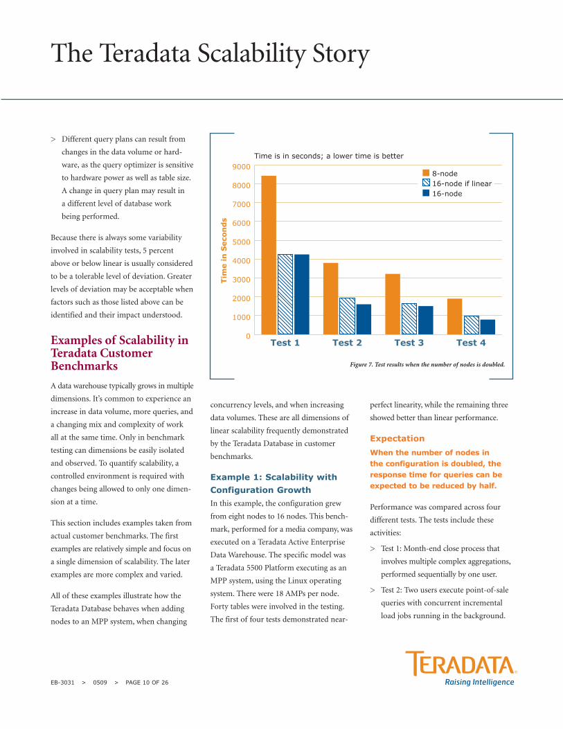
Figure 7. Test results when the number of nodes is doubled.

0

1000

2000

3000

4000

5000

6000

7000

8000

9000

Test 4Test 3Test 2Test 1

Tim

e in

Seco

nd

s

8-node16-node if linear16-node

Time is in seconds; a lower time is better


> Test 3: Same as Test 2, but without the

background load activity.

> Test 4: Single user performs marketing

aggregation query performed on a

cluster of key values.

The total response time in seconds for

each of these four tests on the 8-node

and on the 16-node platform are illus-

trated in Figure 7 with the actual timings

appearing in Table 1. For each of the four

tests, Figure 7 illustrates:

> Total execution time in seconds for the

test with 8 nodes.

> What the expected execution time is

with 16 nodes if scalability is linear.

> Actual total execution time for the test

with 16 nodes.

The data volume was the same in both

of the 8-node and the 16-node tests. Table

1 records the actual response times and

the percent of deviation from linear

scalability.

The same application ran against identical

data for the 8-node test, and then again for

the 16-node test. Different date ranges

were selected for each test. As shown in

Figure 7 and Table 1, Tests 2 and 4 ran

notably better than linear at 16 nodes, com-

pared to their performance at 8 nodes.

One explanation for this better-than-linear

performance is that both Test 2 and Test 4

favored hash joins. When hash joins are

used, it’s possible to achieve better-than-

linear performance when the nodes are

doubled. In this case, when the number

of nodes was doubled, the amount of

memory and the number of AMPs was

also doubled. But because the data volume

remained constant, each AMP had half

as much data to process on the larger

configuration compared to the smaller.

When each AMP has more memory

available for hash joins, the joins will

perform more efficiently by using a larger

number of hash partitions per AMP.

Test 1, on the other hand, was a single large

aggregation job that did not make use of

hash joins, and it demonstrates almost

perfect linear behavior when the nodes

are doubled (8,426 wall-clock seconds

compared to 4,225 wall-clock seconds).

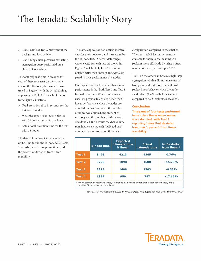
Conclusion

Three out of four tests performedbetter than linear when nodeswere doubled, with Test 1reporting times that deviated less than 1 percent from linearscalability.


EB-3031 > 0509 > PAGE 11 OF 26

8-node time

Expected 16-node time

if linearActual

16-node time% Deviation from linear*

Test 1 8426 4213 4245 0.76%

Test 2 3796 1898 1600 -15.70%

Test 3 3215 1608 1503 -6.53%

Test 4 1899 950 787 -17.16%

* When comparing response times, a negative % indicates better-than-linear performance, and a positive % means worse than linear.

Table 1. Total response time (in seconds) for each of four tests, before and after the nodes were doubled.


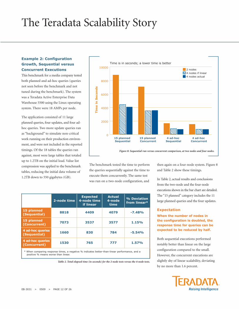
Example 2: ConfigurationGrowth, Sequential versusConcurrent Executions This benchmark for a media company tested

both planned and ad-hoc queries (queries

not seen before the benchmark and not

tuned during the benchmark). The system

was a Teradata Active Enterprise Data

Warehouse 5500 using the Linux operating


The application consisted of 11 large

planned queries, four updates, and four ad-

hoc queries. Two more update queries ran

as “background” to simulate non-critical

work running on their production environ-

ment, and were not included in the reported

timings. Of the 18 tables the queries ran

against, most were large tables that totaled

up to 1.2TB on the initial load. Value list

compression was applied to the benchmark

tables, reducing the initial data volume of

1.2TB down to 550 gigabytes (GB).

The benchmark tested the time to perform

the queries sequentially against the time to

execute them concurrently. The same test

was run on a two-node configuration, and

then again on a four-node system. Figure 8

and Table 2 show these timings.

In Table 2, actual results and conclusions

from the two-node and the four-node

executions shown in the bar chart are detailed.

The “15 planned” category includes the 11

large planned queries and the four updates.

Expectation

When the number of nodes in the configuration is doubled, theresponse time for queries can beexpected to be reduced by half.

Both sequential executions performed

notably better than linear on the large

configuration compared to the small.

However, the concurrent executions are

slightly shy of linear scalability, deviating

by no more than 1.6 percent.


EB-3031 > 0509 > PAGE 12 OF 26

Figure 8: Sequential run versus concurrent comparison, at two nodes and four nodes.

0

2000

4000

6000

8000

10000

4 ad-hoc Concurrent

4 ad-hoc Sequential

15 planned Concurrent

15 planned Sequential

Tim

e in

Seco

nd

s

2 nodes4 nodes if linear4 nodes actual


2-node time Expected

4-node timeif linear

Actual 4-node

time

% Deviationfrom linear*

15 planned(Sequential) 8818 4409 4079 -7.48%

15 planned(Concurrent) 7073 3537 3577 1.15%

4 ad-hoc queries(Sequential) 1660 830 784 -5.54%

4 ad-hoc queries(Concurrent) 1530 765 777 1.57%

* When comparing response times, a negative % indicates better-than-linear performance, and apositive % means worse than linear.

Table 2. Total elapsed time (in seconds) for the 2-node tests versus the 4-node tests.


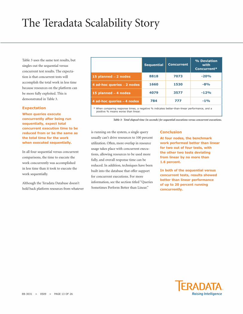
Table 3 uses the same test results, but

singles out the sequential versus

concurrent test results. The expecta-

tion is that concurrent tests will

accomplish the total work in less time

because resources on the platform can

be more fully exploited. This is

demonstrated in Table 3.

Expectation

When queries executeconcurrently after being runsequentially, expect totalconcurrent execution time to bereduced from or be the same asthe total time for the work when executed sequentially.

In all four sequential versus concurrent

comparisons, the time to execute the

work concurrently was accomplished

in less time than it took to execute the

work sequentially.

Although the Teradata Database doesn’t

hold back platform resources from whatever

is running on the system, a single query

usually can’t drive resources to 100 percent

utilization. Often, more overlap in resource

usage takes place with concurrent execu-

tions, allowing resources to be used more

fully, and overall response time can be

reduced. In addition, techniques have been

built into the database that offer support

for concurrent executions. For more

information, see the section titled “Queries

Sometimes Perform Better than Linear.”

Conclusion

At four nodes, the benchmark work performed better than linearfor two out of four tests, with the other two tests deviating from linear by no more than 1.6 percent.

In both of the sequential versusconcurrent tests, results showedbetter than linear performance of up to 20 percent running concurrently.


EB-3031 > 0509 > PAGE 13 OF 26

Sequential Concurrent% Deviation

withConcurrent*

15 planned — 2 nodes 8818 7073 -20%

4 ad-hoc queries — 2 nodes 1660 1530 -8%

15 planned — 4 nodes 4079 3577 -12%

4 ad-hoc queries — 4 nodes 784 777 -1%


Table 3: Total elapsed time (in seconds) for sequential executions versus concurrent executions.


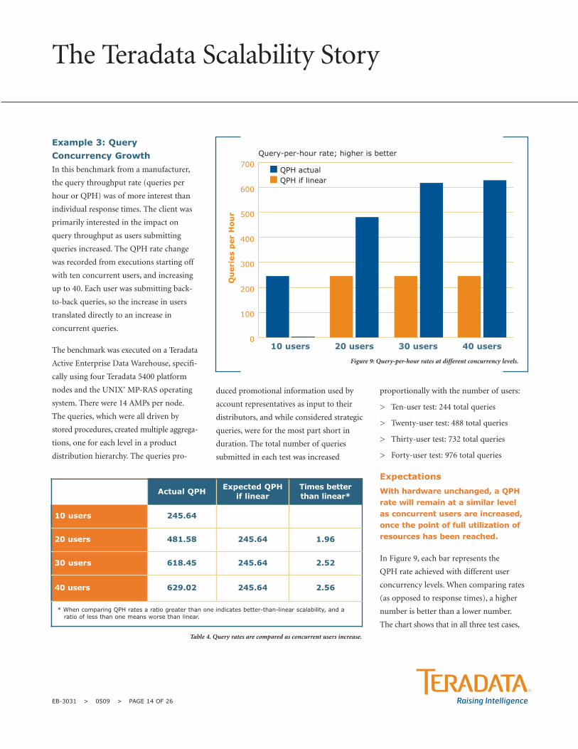
Example 3: QueryConcurrency Growth In this benchmark from a manufacturer,

the query throughput rate (queries per

hour or QPH) was of more interest than

individual response times. The client was

primarily interested in the impact on

query throughput as users submitting

queries increased. The QPH rate change

was recorded from executions starting off

with ten concurrent users, and increasing

up to 40. Each user was submitting back-

to-back queries, so the increase in users

translated directly to an increase in

concurrent queries.

The benchmark was executed on a Teradata

Active Enterprise Data Warehouse, specifi-

cally using four Teradata 5400 platform

nodes and the UNIX® MP-RAS operating


The queries, which were all driven by

stored procedures, created multiple aggrega-

tions, one for each level in a product

distribution hierarchy. The queries pro-

duced promotional information used by

account representatives as input to their

distributors, and while considered strategic

queries, were for the most part short in

duration. The total number of queries

submitted in each test was increased

proportionally with the number of users:

> Ten-user test: 244 total queries

> Twenty-user test: 488 total queries

> Thirty-user test: 732 total queries

> Forty-user test: 976 total queries

Expectations

With hardware unchanged, a QPHrate will remain at a similar levelas concurrent users are increased,once the point of full utilization ofresources has been reached.

In Figure 9, each bar represents the

QPH rate achieved with different user

concurrency levels. When comparing rates

(as opposed to response times), a higher

number is better than a lower number.

The chart shows that in all three test cases,


EB-3031 > 0509 > PAGE 14 OF 26

Figure 9: Query-per-hour rates at different concurrency levels.

0

100

200

300

400

500

600

700

40 users30 users20 users10 users

Qu

eri

es

per

Ho

ur

QPH actualQPH if linear

Query-per-hour rate; higher is better

Actual QPH Expected QPH if linear

Times better than linear*

10 users 245.64

20 users 481.58 245.64 1.96

30 users 618.45 245.64 2.52

40 users 629.02 245.64 2.56

* When comparing QPH rates a ratio greater than one indicates better-than-linear scalability, and a ratio of less than one means worse than linear.

Table 4. Query rates are compared as concurrent users increase.


when users were increased beyond the

baseline of ten, throughput increased

beyond expectation. That’s because it took

at least 30 of their concurrent queries to

begin to fully utilize the resources of the

system in this benchmark.

Table 4 presents the actual query rates that

were achieved across the four tests. The

column labeled Times better than linear

calculates the ratio of the query rate for

that user concurrency level compared to

the original ten-user query rate.

The query rate almost doubled going from

ten to 20 users, and was 2.5 times higher

going from ten to 30 users. This is because

platform resources were only moderately

used with ten users actively submitting

queries. As more users became active,

there were still available resources that

could be applied to the new work driving

the query completion rate higher. When

30 users were active, resources were more

fully utilized, as you can see by the very

minimal improvement of the QPH rate

with 40 users compared to the QPH rate

of 30 users (629.02/618.45 = 1.017 or 2

percent). Because one of the goals of this

benchmark was to get the query work done

as quickly as possible, concurrency was not

increased beyond 40, which was considered

the point at which peak throughput was

reached for this application.

Conclusion

Better-than-linear query through-put was demonstrated across alltests, as users submitting querieswere increased from ten up to 40.

Example 4: Data VolumeGrowth This benchmark example from a retailer

examines the impact of data volume

increases on query response times. In this

case, the ad-hoc MSI queries and customer

SQL queries were executed sequentially

at the base volume and then again at a

higher volume, referred to here as “Base * 3.”

This benchmark was executed on a Teradata

Active Enterprise Data Warehouse, specifi-

cally a four-node Teradata Active Enterprise

Data Warehouse 5500 using the Linux

operating system. There were 18 AMPs

per node.

As is usually the case in the real world, table

growth within this benchmark was uneven.

The queries were executed on actual

customer data, not fabricated data, so the

increase in the number of rows of each

table was slightly different. Queries that

perform full table scans will be more sensi-

tive to changes in the number of rows in the

table. Queries that perform indexed access

are likely to be less sensitive to such changes.

Expectation

When the data volume is increased,all-AMP queries can be expected to demonstrate a change inresponse time that is proportionalto the data volume increase.

The data growth details are shown in Table

5. Overall tables increased from a low of

two times more rows to a high of three

times more rows. Two of the larger tables

(the two fact tables) increased their row

counts by slightly more than three times.

Total volume went from 7.5 billion rows

to 23 billion rows, slightly more than three

times larger.

Notice that the large fact table (Inventory_

Fact) grew almost exactly three times, as

did the Order_Log_Hdr and Order_Log_

Dtl. Smaller dimension tables were

increased between two and three times.

Even though the two fact tables were more

than three times larger, the actual effort to

process data from the fact tables was about

double because the fact tables were defined

using partitioned primary index (PPI).

When a query that provides partitioning

information accesses a PPI table, table

scan activity can be reduced to a subset of

the table’s partitions. This shortens such a

query’s execution time and can blur linear

scalability assessments.

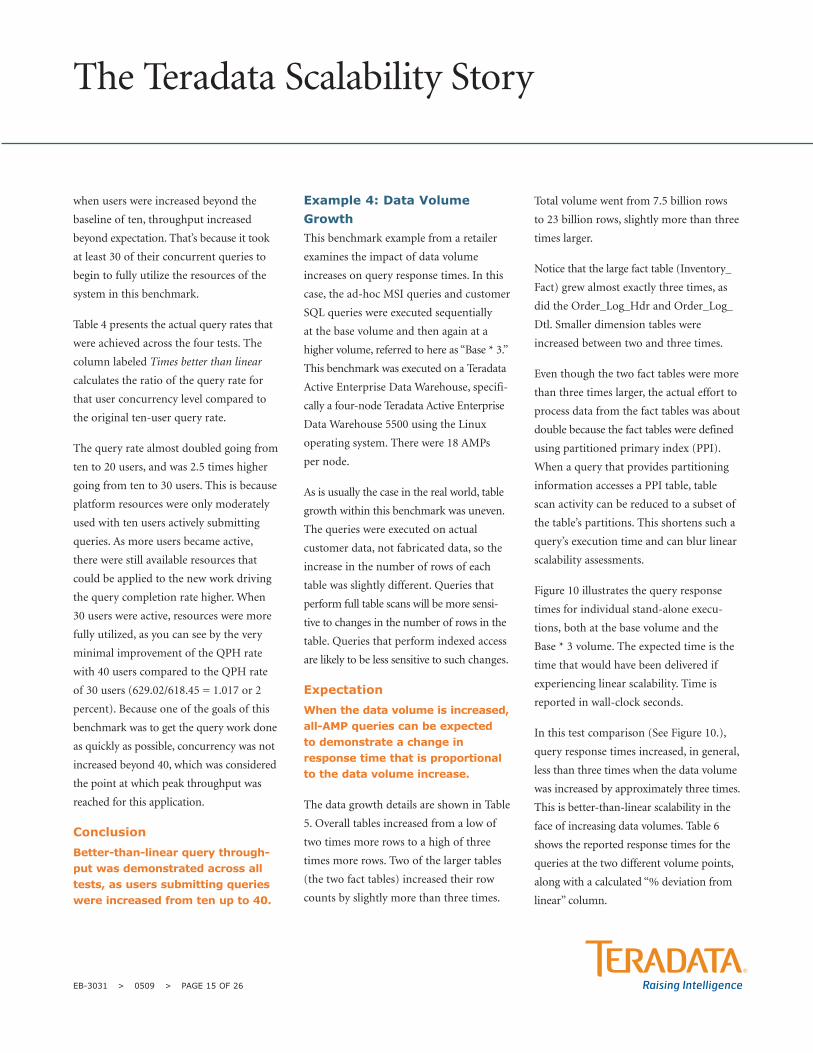
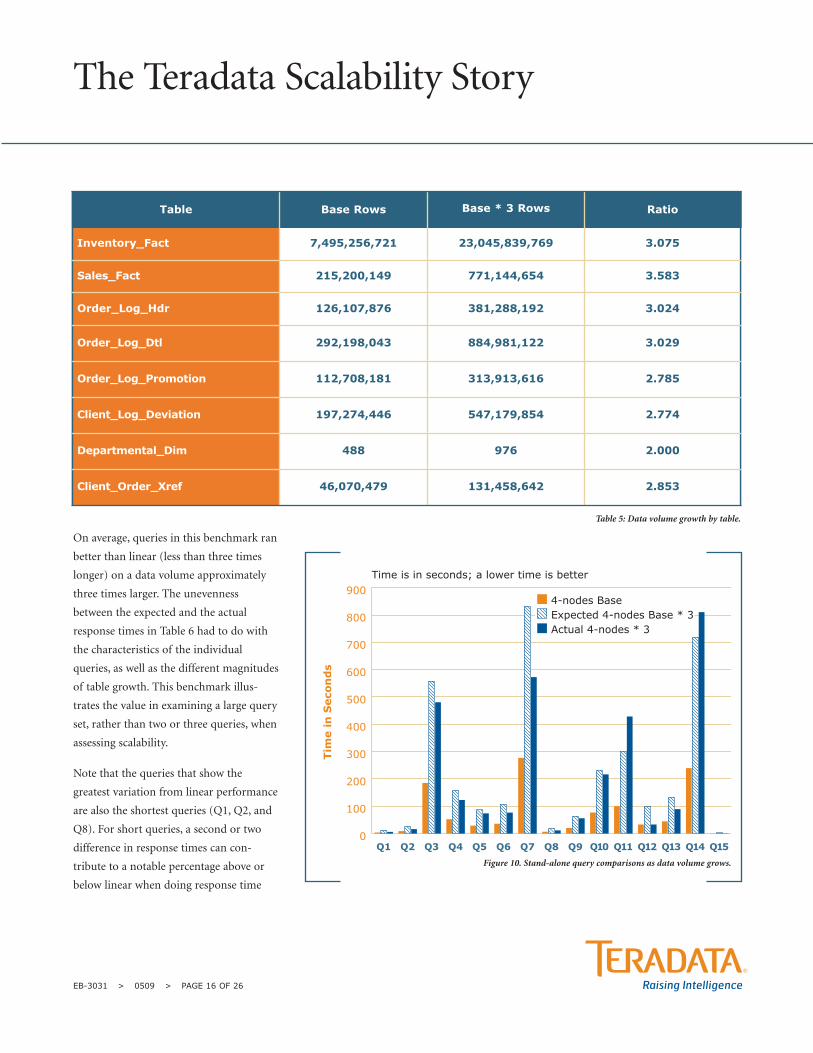
Figure 10 illustrates the query response

times for individual stand-alone execu-

tions, both at the base volume and the

Base * 3 volume. The expected time is the

time that would have been delivered if

experiencing linear scalability. Time is

reported in wall-clock seconds.

In this test comparison (See Figure 10.),

query response times increased, in general,

less than three times when the data volume

was increased by approximately three times.

This is better-than-linear scalability in the

face of increasing data volumes. Table 6

shows the reported response times for the

queries at the two different volume points,

along with a calculated “% deviation from

linear” column.


EB-3031 > 0509 > PAGE 15 OF 26


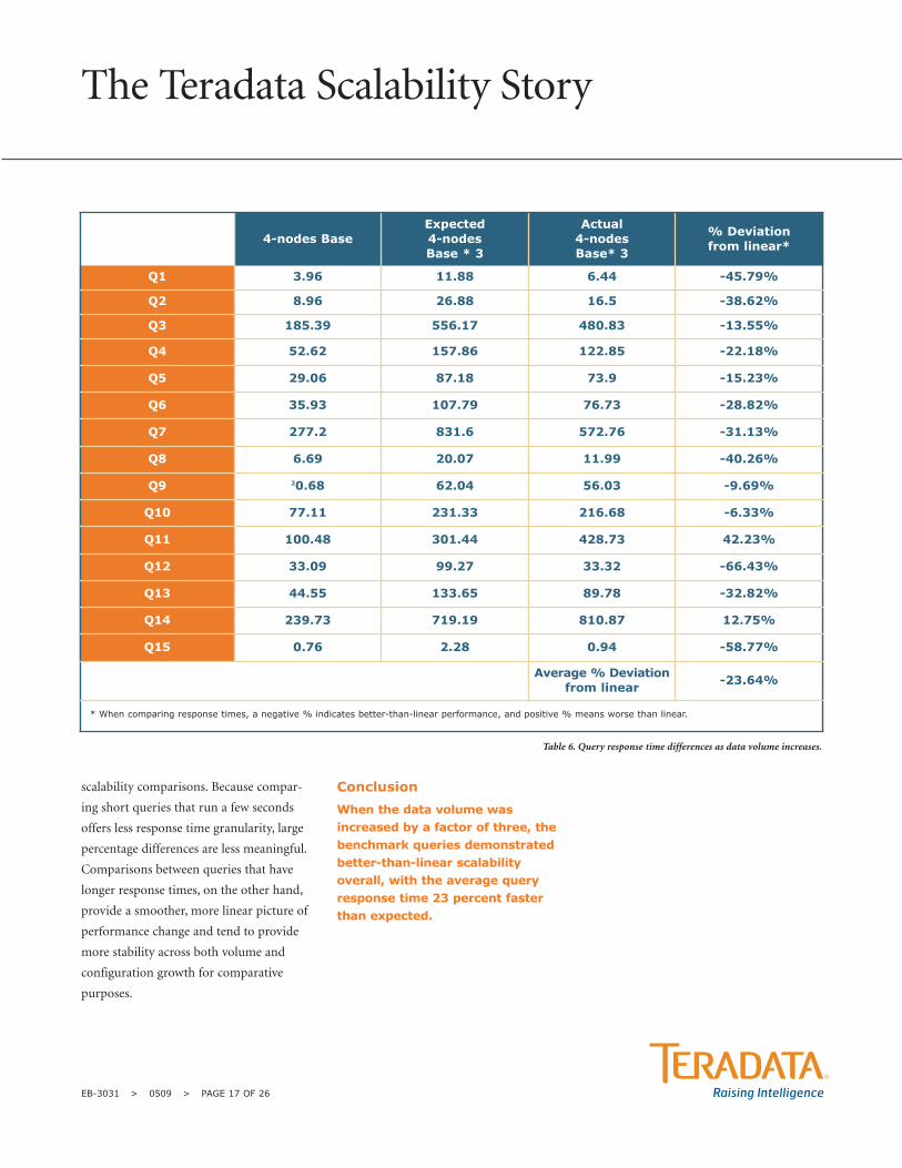
On average, queries in this benchmark ran

better than linear (less than three times

longer) on a data volume approximately

three times larger. The unevenness

between the expected and the actual

response times in Table 6 had to do with

the characteristics of the individual

queries, as well as the different magnitudes

of table growth. This benchmark illus-

trates the value in examining a large query

set, rather than two or three queries, when

assessing scalability.

Note that the queries that show the

greatest variation from linear performance

are also the shortest queries (Q1, Q2, and

Q8). For short queries, a second or two

difference in response times can con-

tribute to a notable percentage above or

below linear when doing response time


EB-3031 > 0509 > PAGE 16 OF 26

Table Base Rows Base * 3 Rows Ratio

Inventory_Fact 7,495,256,721 23,045,839,769 3.075

Sales_Fact 215,200,149 771,144,654 3.583

Order_Log_Hdr 126,107,876 381,288,192 3.024

Order_Log_Dtl 292,198,043 884,981,122 3.029

Order_Log_Promotion 112,708,181 313,913,616 2.785

Client_Log_Deviation 197,274,446 547,179,854 2.774

Departmental_Dim 488 976 2.000

Client_Order_Xref 46,070,479 131,458,642 2.853

Table 5: Data volume growth by table.

Figure 10. Stand-alone query comparisons as data volume grows.

0

100

200

300

400

500

600

700

800

900

Q15Q14Q13Q12Q11Q10Q9Q8Q7Q6Q5Q4Q3Q2Q1

Tim

e in

Seco

nd

s

4-nodes BaseExpected 4-nodes Base * 3Actual 4-nodes * 3



scalability comparisons. Because compar-

ing short queries that run a few seconds

offers less response time granularity, large

percentage differences are less meaningful.

Comparisons between queries that have

longer response times, on the other hand,

provide a smoother, more linear picture of

performance change and tend to provide

more stability across both volume and

configuration growth for comparative

purposes.

Conclusion

When the data volume wasincreased by a factor of three, thebenchmark queries demonstratedbetter-than-linear scalabilityoverall, with the average queryresponse time 23 percent fasterthan expected.


EB-3031 > 0509 > PAGE 17 OF 26

Table 6. Query response time differences as data volume increases.

4-nodes Base Expected 4-nodes Base * 3

Actual 4-nodes Base* 3

% Deviation from linear*

Q1 3.96 11.88 6.44 -45.79%

Q2 8.96 26.88 16.5 -38.62%

Q3 185.39 556.17 480.83 -13.55%

Q4 52.62 157.86 122.85 -22.18%

Q5 29.06 87.18 73.9 -15.23%

Q6 35.93 107.79 76.73 -28.82%

Q7 277.2 831.6 572.76 -31.13%

Q8 6.69 20.07 11.99 -40.26%

Q9 20.68 62.04 56.03 -9.69%

Q10 77.11 231.33 216.68 -6.33%

Q11 100.48 301.44 428.73 42.23%

Q12 33.09 99.27 33.32 -66.43%

Q13 44.55 133.65 89.78 -32.82%

Q14 239.73 719.19 810.87 12.75%

Q15 0.76 2.28 0.94 -58.77%

Average % Deviation from linear -23.64%

* When comparing response times, a negative % indicates better-than-linear performance, and positive % means worse than linear.


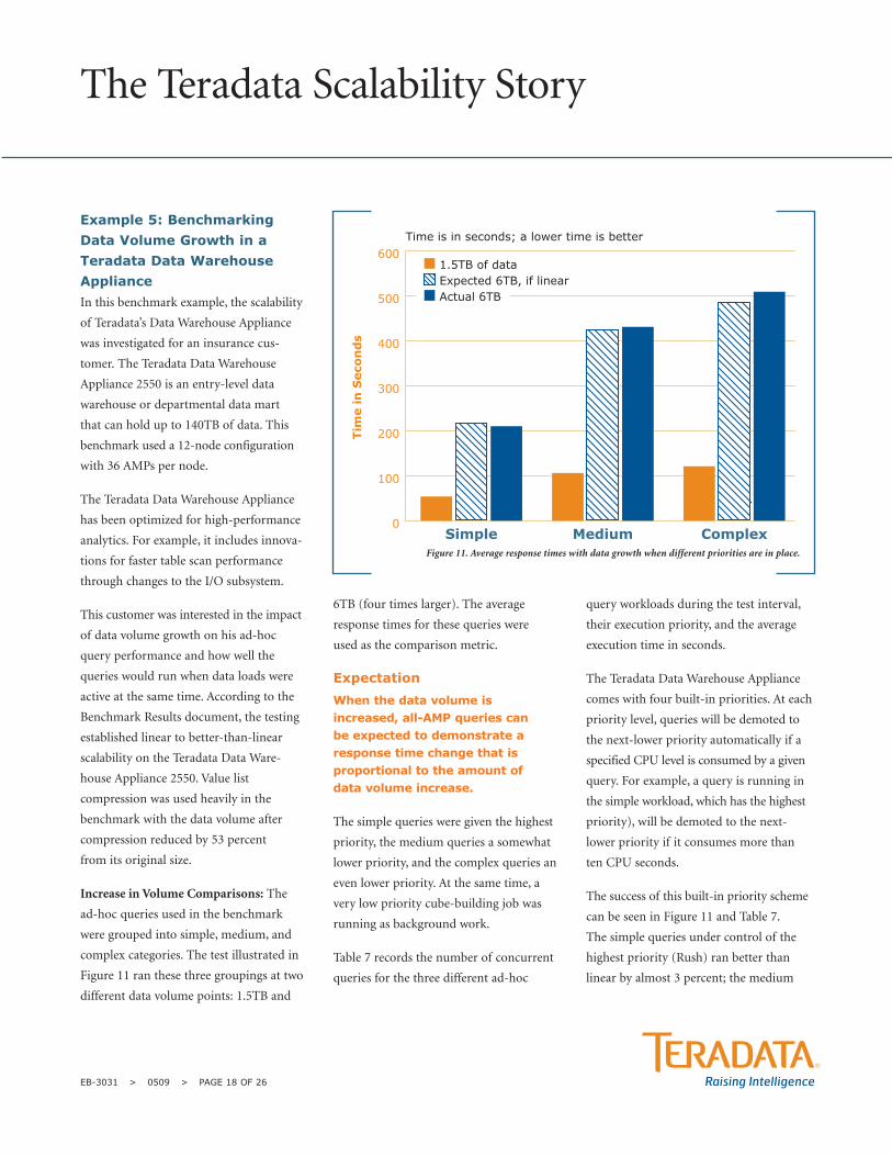
Example 5: BenchmarkingData Volume Growth in aTeradata Data WarehouseAppliance In this benchmark example, the scalability

of Teradata’s Data Warehouse Appliance

was investigated for an insurance cus-

tomer. The Teradata Data Warehouse

Appliance 2550 is an entry-level data

warehouse or departmental data mart

that can hold up to 140TB of data. This

benchmark used a 12-node configuration

with 36 AMPs per node.

The Teradata Data Warehouse Appliance

has been optimized for high-performance

analytics. For example, it includes innova-

tions for faster table scan performance

through changes to the I/O subsystem.

This customer was interested in the impact

of data volume growth on his ad-hoc

query performance and how well the

queries would run when data loads were

active at the same time. According to the

Benchmark Results document, the testing

established linear to better-than-linear

scalability on the Teradata Data Ware-

house Appliance 2550. Value list

compression was used heavily in the

benchmark with the data volume after

compression reduced by 53 percent

from its original size.

Increase in Volume Comparisons: The

ad-hoc queries used in the benchmark

were grouped into simple, medium, and

complex categories. The test illustrated in

Figure 11 ran these three groupings at two

different data volume points: 1.5TB and

6TB (four times larger). The average

response times for these queries were

used as the comparison metric.

Expectation

When the data volume isincreased, all-AMP queries can be expected to demonstrate aresponse time change that isproportional to the amount of data volume increase.

The simple queries were given the highest

priority, the medium queries a somewhat

lower priority, and the complex queries an

even lower priority. At the same time, a

very low priority cube-building job was

running as background work.

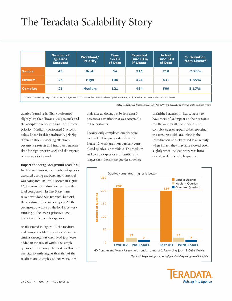
Table 7 records the number of concurrent

queries for the three different ad-hoc

query workloads during the test interval,

their execution priority, and the average

execution time in seconds.

The Teradata Data Warehouse Appliance

comes with four built-in priorities. At each

priority level, queries will be demoted to

the next-lower priority automatically if a

specified CPU level is consumed by a given

query. For example, a query is running in

the simple workload, which has the highest

priority), will be demoted to the next-

lower priority if it consumes more than

ten CPU seconds.

The success of this built-in priority scheme

can be seen in Figure 11 and Table 7.

The simple queries under control of the

highest priority (Rush) ran better than

linear by almost 3 percent; the medium


EB-3031 > 0509 > PAGE 18 OF 26

Figure 11. Average response times with data growth when different priorities are in place.

0

100

200

300

400

500

600

ComplexMediumSimple

Tim

e in

Seco

nd

s

1.5TB of dataExpected 6TB, if linearActual 6TB



queries (running in High) performed

slightly less than linear (1.65 percent); and

the complex queries running at the lowest

priority (Medium) performed 5 percent

below linear. In this benchmark, priority

differentiation is working effectively

because it protects and improves response

time for high-priority work and the expense

of lower-priority work.

Impact of Adding Background Load Jobs:

In this comparison, the number of queries

executed during the benchmark interval

was compared. In Test 2, shown in Figure

12, the mixed workload ran without the

load component. In Test 3, the same

mixed workload was repeated, but with

the addition of several load jobs. All the

background work and the load jobs were

running at the lowest priority (Low),

lower than the complex queries.

As illustrated in Figure 12, the medium

and complex ad-hoc queries sustained a

similar throughput when load jobs were

added to the mix of work. The simple

queries, whose completion rate in this test

was significantly higher than that of the

medium and complex ad-hoc work, saw

their rate go down, but by less than 5

percent, a deviation that was acceptable

to the customer.

Because only completed queries were

counted in the query rates shown in

Figure 12, work spent on partially com-

pleted queries is not visible. The medium

and complex queries ran significantly

longer than the simple queries allowing

unfinished queries in that category to

have more of an impact on their reported

results. As a result, the medium and

complex queries appear to be reporting

the same rate with and without the

introduction of background load activity,

when in fact, they may have slowed down

slightly when the load work was intro-

duced, as did the simple queries.


EB-3031 > 0509 > PAGE 19 OF 26

Table 7. Response times (in seconds) for different priority queries as data volume grows.

Number ofQueries

Executed

Workload/Priority

Time1.5TB

of Data

ExpectedTime 6TB, if Linear

ActualTime 6TBof Data

% Deviationfrom Linear*

Simple 49 Rush 54 216 210 -2.78%

Medium 25 High 106 424 431 1.65%

Complex 25 Medium 121 484 509 5.17%


Figure 12: Impact on query throughput of adding background load jobs.

0

50

100

150

200

250

Test #3 – With LoadsTest #2 – No Loads

Nu

mb

er

of

Qu

eri

es

Simple QueriesMedium QueriesComplex Queries

Queries completed; higher is better

40 Concurrent Query Users, with background of 2 Reporting jobs, 2 Cube Builds

207

177

177

197


The load jobs in this test were running at a

low priority – the same low priority as the

reporting jobs and cube builds that were also

going on at the same time. The reporting

jobs performed very large summarizations

for six different evaluation periods, scanning

all records from fact and dimension tables

and requiring spool space in excess of

1.3TB. The higher priority of the query

work helped to protect their throughput

rates even in the face of increased compe-

tition for platform resources.

Conclusion

The high priority ad-hoc queriesran better than linear by almost 3percent when data volume wasincreased by a factor of four, whilethe medium and lower priorityqueries deviated slightly fromlinear, by 2 percent and 5 percent,respectively.

Example 6: Increasing DataVolume and Node Hardware This benchmark from a client in the travel

business tested different volumes on

differently sized configurations on two

Teradata Active Enterprise Data Ware-

houses. Performance on a six-node Teradata

5550 Platform was compared to that on a

12-node Teradata 5550 Platform, both using

the Linux operating system. Both configura-

tions had 25 AMPs per node. The data

volume was varied from 10TB to 20TB.

The benchmark test was representative of

a typical active data warehouse with its

ongoing load activity, its mix of work that

included tactical queries, and its use of

workload management. Thirty different

long-running, complex analytic queries,

and five different moderate reporting

queries, as well as three different sets of

tactical queries, made up the test applica-

tion. At the same time as the execution

of these queries, incremental loads into

18 tables were taking place. More than

300 sessions were active during the test

interval of two hours.

The Merchant Tactical queries were exclu-

sively single-AMP queries. The Operational

Reporting, Quick Response, and Client

History tactical query sets were primarily

single-AMP, but supported some level of

all-AMP queries as well.

Expectation

When both the number of nodesand the volume of data increase tothe same degree, expect the queryresponse times for all-AMP queriesto be similar.

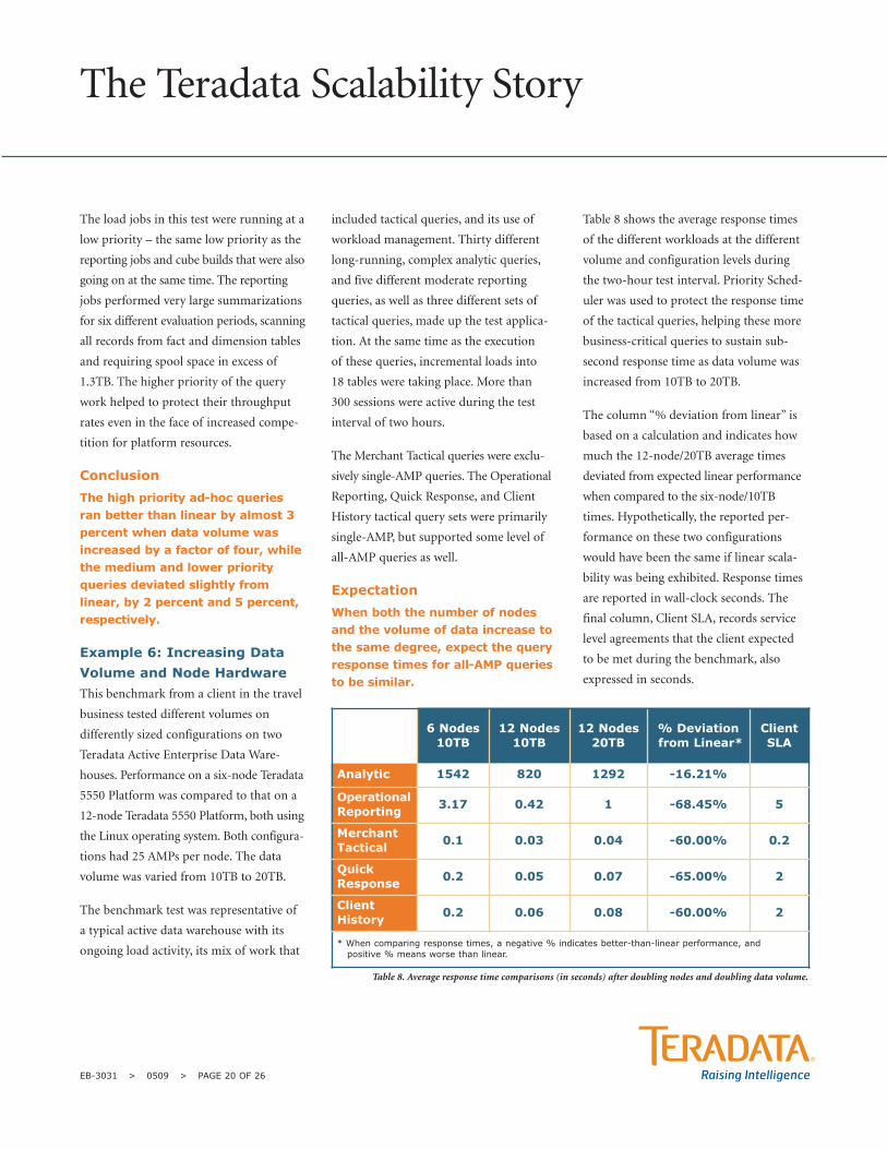
Table 8 shows the average response times

of the different workloads at the different

volume and configuration levels during

the two-hour test interval. Priority Sched-

uler was used to protect the response time

of the tactical queries, helping these more

business-critical queries to sustain sub-

second response time as data volume was

increased from 10TB to 20TB.

The column “% deviation from linear” is

based on a calculation and indicates how

much the 12-node/20TB average times

deviated from expected linear performance

when compared to the six-node/10TB

times. Hypothetically, the reported per-

formance on these two configurations

would have been the same if linear scala-

bility was being exhibited. Response times

are reported in wall-clock seconds. The

final column, Client SLA, records service

level agreements that the client expected

to be met during the benchmark, also

expressed in seconds.


EB-3031 > 0509 > PAGE 20 OF 26

Table 8. Average response time comparisons (in seconds) after doubling nodes and doubling data volume.

6 Nodes10TB

12 Nodes10TB

12 Nodes20TB


ClientSLA

Analytic 1542 820 1292 -16.21%

OperationalReporting 3.17 0.42 1 -68.45% 5

MerchantTactical 0.1 0.03 0.04 -60.00% 0.2

QuickResponse 0.2 0.05 0.07 -65.00% 2

ClientHistory 0.2 0.06 0.08 -60.00% 2



All workloads in this benchmark demon-

strated better-than-linear performance

when both the data volume and the number

of nodes doubled. However, among the

different workloads, the analytic queries

showed closer to linear behavior perform-

ing better than linear by only 16 percent.

Why Analytic Queries Performed Better

than Linear: At the 20TB volume point,

the analytic queries were able to perform

somewhat better than linear, because the

tables they accessed were defined with PPI.

Some of the analytic queries took advan-

tage of this partitioning. When, due to

partitioning, only a subset of a table’s rows

has to scanned, an increase in the total

rows in the table may have less impact on

a query’s response time.

Why Tactical Queries Performed Better

than Linear: As shown in Table 8, these

results exceeded the customer’s tactical

query service level agreements (SLA) by

as much as 20 times on all configurations.

As an example, the Client History’s SLA

of 2.0 seconds was more than satisfied by

an average response time in the benchmark

of 0.08 seconds on the 12-node/20TB

configuration. In addition to exceeding

response time expectations at all test levels,

the scalability between the different test

configurations proved better than expected.

There are two explanations for why the

tactical workload average times performed

better than linear to such a degree (60 to

65 percent):

1. Most of the queries in these three

tactical workloads were single-AMP,

direct access queries (Merchant Tactical

were exclusively single-AMP). Because

such queries are localized to a single

AMP and do not access data across all

AMPs, when the configuration grows

and more nodes are added (and second-

arily, more AMPs), a greater number of

such queries can execute at the same

time without any response time degra-

dation. This is possible because the

work is spread across a greater number

of AMPs and nodes, diluting any

competition for resources within the

workload. In addition, as data volume

increases, single-AMP queries are not

penalized because the effort to access

one or a few rows on a single AMP

remains the same, regardless of volume.

2. In this benchmark, tactical queries

were given a higher priority, which

protects their short response time and

high query rates as data volume grows

and as contention for resources

increases on the system due to other

queries having more work to do.

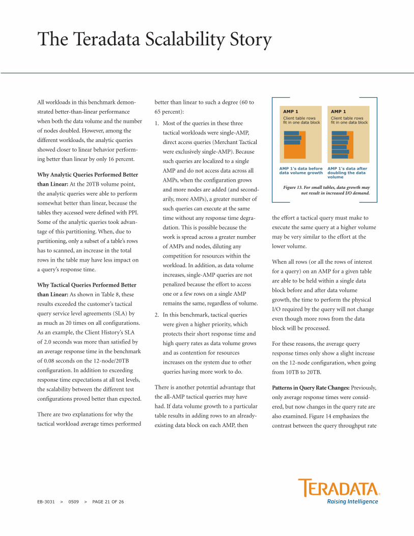
There is another potential advantage that

the all-AMP tactical queries may have

had. If data volume growth to a particular

table results in adding rows to an already-

existing data block on each AMP, then

the effort a tactical query must make to

execute the same query at a higher volume

may be very similar to the effort at the

lower volume.

When all rows (or all the rows of interest

for a query) on an AMP for a given table

are able to be held within a single data

block before and after data volume

growth, the time to perform the physical

I/O required by the query will not change

even though more rows from the data

block will be processed.

For these reasons, the average query

response times only show a slight increase

on the 12-node configuration, when going

from 10TB to 20TB.

Patterns in Query Rate Changes: Previously,

only average response times were consid-

ered, but now changes in the query rate are

also examined. Figure 14 emphasizes the

contrast between the query throughput rate


EB-3031 > 0509 > PAGE 21 OF 26

Figure 13. For small tables, data growth maynot result in increased I/O demand.

AMP 1Client table rowsfit in one data block

AMP 1’s data beforedata volume growth

AMP 1’s data afterdoubling the data volume

AMP 1Client table rowsfit in one data block


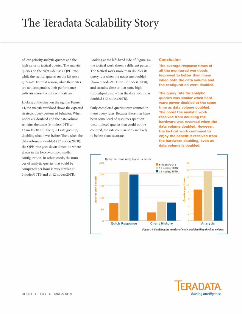
of low-priority analytic queries and the

high-priority tactical queries. The analytic

queries on the right side use a QPH rate,

while the tactical queries on the left use a

QPS rate. For that reason, while their rates

are not comparable, their performance

patterns across the different tests are.

Looking at the chart on the right in Figure

14, the analytic workload shows the expected

strategic query pattern of behavior. When

nodes are doubled and the data volume

remains the same (6 nodes/10TB to

12 nodes/10TB), the QPH rate goes up,

doubling what it was before. Then, when the

data volume is doubled (12 nodes/20TB),

the QPH rate goes down almost to where

it was in the lower-volume, smaller

configuration. In other words, the num-

ber of analytic queries that could be

completed per hour is very similar at

6 nodes/10TB and at 12 nodes/20TB.

Looking at the left-hand side of Figure 14,

the tactical work shows a different pattern.

The tactical work more than doubles its

query rate when the nodes are doubled

(from 6 nodes/10TB to 12 nodes/10TB),

and sustains close to that same high

throughput even when the data volume is

doubled (12 nodes/20TB).

Only completed queries were counted in

these query rates. Because there may have

been some level of resources spent on

uncompleted queries that could not be

counted, the rate comparisons are likely

to be less than accurate.

Conclusion

The average response times of all the monitored workloadsimproved to better than linearwhen both the data volume andthe configuration were doubled.

The query rate for analytic queries was similar when hard-ware power doubled at the sametime as data volume doubled. The boost the analytic workreceived from doubling thehardware was reversed when thedata volume doubled. However,the tactical work continued toenjoy the benefit it received fromthe hardware doubling, even asdata volume is doubled.


EB-3031 > 0509 > PAGE 22 OF 26

0

50

100

150

200

250

Client HistoryQuick Response

Qu

eri

es

per

Seco

nd

6 nodes/10TB12 nodes/10TB12 nodes/20TB

Query-per-time rate; higher is better

0

2

4

6

8

10

12

14

16

Analytic

Qu

eri

es

per

Ho

ur

Figure 14. Doubling the number of nodes and doubling the data volume.


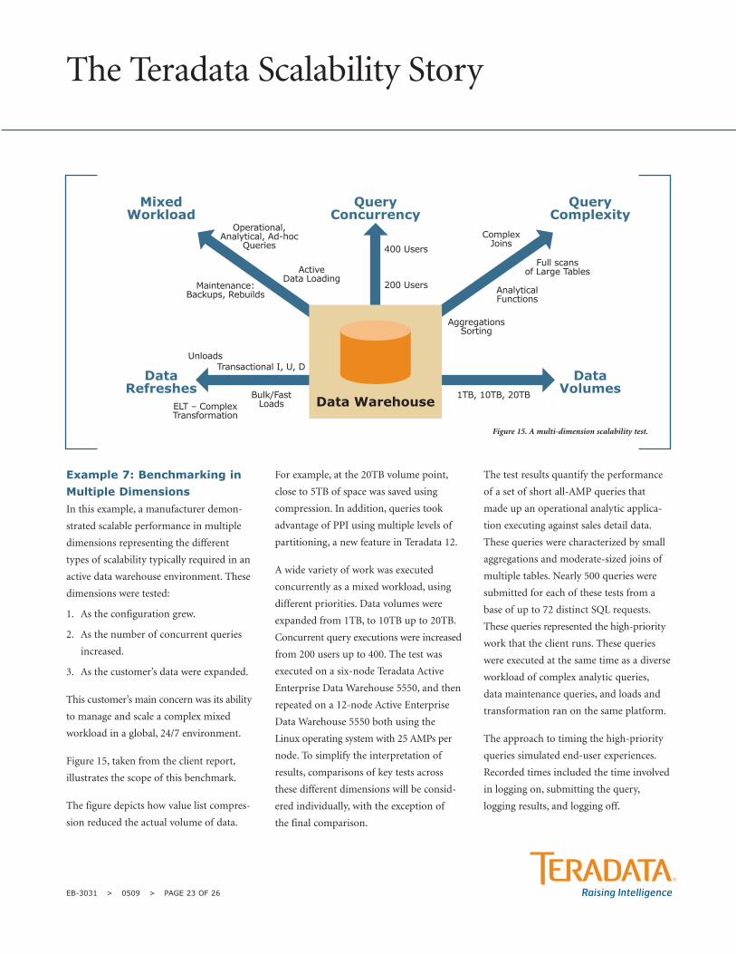
Example 7: Benchmarking inMultiple Dimensions In this example, a manufacturer demon-

strated scalable performance in multiple

dimensions representing the different

types of scalability typically required in an

active data warehouse environment. These

dimensions were tested:

1. As the configuration grew.

2. As the number of concurrent queries

increased.

3. As the customer’s data were expanded.

This customer’s main concern was its ability

to manage and scale a complex mixed

workload in a global, 24/7 environment.

Figure 15, taken from the client report,

illustrates the scope of this benchmark.

The figure depicts how value list compres-

sion reduced the actual volume of data.

For example, at the 20TB volume point,

close to 5TB of space was saved using

compression. In addition, queries took

advantage of PPI using multiple levels of

partitioning, a new feature in Teradata 12.

A wide variety of work was executed

concurrently as a mixed workload, using

different priorities. Data volumes were

expanded from 1TB, to 10TB up to 20TB.

Concurrent query executions were increased

from 200 users up to 400. The test was

executed on a six-node Teradata Active

Enterprise Data Warehouse 5550, and then

repeated on a 12-node Active Enterprise

Data Warehouse 5550 both using the

Linux operating system with 25 AMPs per

node. To simplify the interpretation of

results, comparisons of key tests across

these different dimensions will be consid-

ered individually, with the exception of

the final comparison.

The test results quantify the performance

of a set of short all-AMP queries that

made up an operational analytic applica-

tion executing against sales detail data.

These queries were characterized by small

aggregations and moderate-sized joins of

multiple tables. Nearly 500 queries were

submitted for each of these tests from a

base of up to 72 distinct SQL requests.

These queries represented the high-priority

work that the client runs. These queries

were executed at the same time as a diverse

workload of complex analytic queries,

data maintenance queries, and loads and

transformation ran on the same platform.

The approach to timing the high-priority

queries simulated end-user experiences.

Recorded times included the time involved

in logging on, submitting the query,

logging results, and logging off.


EB-3031 > 0509 > PAGE 23 OF 26

Figure 15. A multi-dimension scalability test.

DataVolumes

QueryComplexity

DataRefreshes

MixedWorkload

QueryConcurrency

Data Warehouse1TB, 10TB, 20TB

AggregationsSorting

AnalyticalFunctions

Full scansof Large Tables

ComplexJoins

400 Users

200 Users

Operational,Analytical, Ad-hoc

Queries

ActiveData Loading

Maintenance:Backups, Rebuilds

UnloadsTransactional I, U, D

Bulk/FastLoadsELT – Complex

Transformation


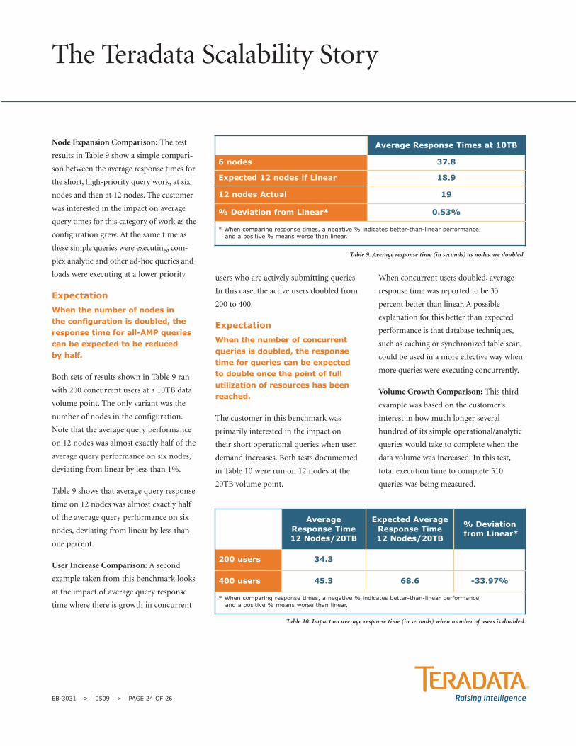
Node Expansion Comparison: The test

results in Table 9 show a simple compari-

son between the average response times for

the short, high-priority query work, at six

nodes and then at 12 nodes. The customer

was interested in the impact on average

query times for this category of work as the

configuration grew. At the same time as

these simple queries were executing, com-

plex analytic and other ad-hoc queries and

loads were executing at a lower priority.

Expectation

When the number of nodes in the configuration is doubled, theresponse time for all-AMP queriescan be expected to be reduced by half.

Both sets of results shown in Table 9 ran

with 200 concurrent users at a 10TB data

volume point. The only variant was the

number of nodes in the configuration.

Note that the average query performance

on 12 nodes was almost exactly half of the

average query performance on six nodes,

deviating from linear by less than 1%.

Table 9 shows that average query response

time on 12 nodes was almost exactly half

of the average query performance on six

nodes, deviating from linear by less than

one percent.

User Increase Comparison: A second

example taken from this benchmark looks

at the impact of average query response

time where there is growth in concurrent

users who are actively submitting queries.

In this case, the active users doubled from

200 to 400.

Expectation

When the number of concurrentqueries is doubled, the responsetime for queries can be expected to double once the point of fullutilization of resources has beenreached.

The customer in this benchmark was

primarily interested in the impact on

their short operational queries when user

demand increases. Both tests documented

in Table 10 were run on 12 nodes at the

20TB volume point.

When concurrent users doubled, average

response time was reported to be 33

percent better than linear. A possible

explanation for this better than expected

performance is that database techniques,

such as caching or synchronized table scan,

could be used in a more effective way when

more queries were executing concurrently.

Volume Growth Comparison: This third

example was based on the customer’s

interest in how much longer several

hundred of its simple operational/analytic

queries would take to complete when the

data volume was increased. In this test,

total execution time to complete 510

queries was being measured.

Average Response Times at 10TB

6 nodes 37.8

Expected 12 nodes if Linear 18.9

12 nodes Actual 19

% Deviation from Linear* 0.53%


Table 9. Average response time (in seconds) as nodes are doubled.


EB-3031 > 0509 > PAGE 24 OF 26

AverageResponse Time12 Nodes/20TB

Expected AverageResponse Time 12 Nodes/20TB


200 users 34.3

400 users 45.3 68.6 -33.97%


Table 10. Impact on average response time (in seconds) when number of users is doubled.


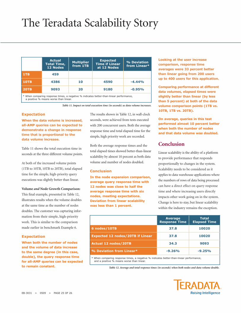
Expectation

When the data volume is increased,all-AMP queries can be expected todemonstrate a change in responsetime that is proportional to thedata volume increase.

Table 11 shows the total execution time in

seconds at the three different volume points.

At both of the increased volume points

(1TB to 10TB, 10TB to 20TB), total elapsed

time for the simple, high-priority query

executions was slightly better than linear.

Volume and Node Growth Comparison:

This final example, presented in Table 12,

illustrates results when the volume doubles

at the same time as the number of nodes

doubles. The customer was capturing infor-

mation from their simple, high-priority

work. This is similar to the comparison

made earlier in benchmark Example 6.

Expectation

When both the number of nodesand the volume of data increase to the same degree (in this case,double), the query response timefor all-AMP queries can be expectedto remain constant.

The results shown in Table 12, in wall-clock

seconds, were achieved from tests executed

with 200 concurrent users. Both the average

response time and total elapsed time for the

simple, high priority work are recorded.

Both the average response times and the

total elapsed times showed better-than-linear

scalability by almost 10 percent as both data

volume and number of nodes doubled.

Conclusion

In the node expansion comparison,average query response time with12 nodes was close to half theaverage response time with sixnodes, meeting expectations.Deviation from linear scalabilitywas less than 1 percent.

Looking at the user increasecomparison, response timeaverages were 33 percent betterthan linear going from 200 users up to 400 users for this application.

Comparing performance at differentdata volumes, elapsed times wereslightly better than linear (by lessthan 5 percent) at both of the datavolume comparison points (1TB vs.10TB, 1TB vs. 20TB).

On average, queries in this testperformed almost 10 percent betterwhen both the number of nodesand that data volume was doubled.

Conclusion

Linear scalability is the ability of a platform

to provide performance that responds

proportionally to changes in the system.

Scalability needs to be considered as it

applies to data warehouse applications where

the numbers of rows of data being processed

can have a direct effect on query response

time and where increasing users directly

impacts other work going on in the system.

Change is here to stay, but linear scalability

within the industry remains the exception.


EB-3031 > 0509 > PAGE 25 OF 26

Actual Total Time,12 Nodes

Multiplierfrom 1TB

ExpectedTime if Linear at 12 Nodes


1TB 459

10TB 4386 10 4590 -4.44%

20TB 9093 20 9180 -0.95%

* When comparing response times, a negative % indicates better-than-linear performance, a positive % means worse than linear.

Table 11. Impact on total execution time (in seconds) as data volume increases.

AverageResponse Time

TotalElapsed Time

6 nodes/10TB 37.8 10020

Expected 12 nodes/20TB if Linear 37.8 10020

Actual 12 nodes/20TB 34.3 9093

% Deviation from Linear* -9.26% -9.25%


Table 12. Average and total response times (in seconds) when both nodes and data volume double.


Illustrating the existence of linear scalability

can be a challenge. None of the bench-

mark examples included in this paper, for

example, provide perfect showcases of

linear scalability across all tests. Some

results were better than linear, many results

were very close to linear, and other results

deviated slightly from linear.

> While the majority of the tests showing

scalability with configuration growth in

Example 1 and Example 2 demonstrated

better-than-linear performance, there

were three comparisons where devia-

tions from linear were reported in the

0.5 to 1.6 percent range.

> Benchmarks examining performance

with data volume growth reported

linear scalability and above across two

different benchmark examples. Average

query response time change in Exam-

ple 4 was more than 20 percent better

than linear. In Example 5, high-priority

queries performed better than linear by

almost 3 percent, while queries in the

lower two priorities deviated from

linear in the 2 to 5.5 percent range,

an expected difference when using

contrasting priorities.

> Better-than-linear performance was

observed when users were increased

from ten to 40 in Example 3, and when

sequential tests were compared against

concurrent tests in Example 2.

> When both hardware growth and data

volume growth increased proportion-

ally in Example 6, better-than-scalable

performance (in the 16 to 68 percent

range) was observed.

> The majority of tests in the three-

dimension scalability comparisons in

Example 7 showed better-than-linear

performance, exceptions varied from

linear by only one half of 1 percent.

Taken in their entirety, these results

make a compelling case for the Teradata

Database’s scalability story.

The Teradata Database system is unique in

its ability to deliver linear scalability as the

number of users increases, as volume

grows, and as the MPP system expands, as

evidenced by examining customer bench-

mark results. This makes non-disruptive

growth possible, enables quicker turn-

around on new user requests, builds

confidence in the quality of the informa-

tion being provided, and offers relief from

the fear of too much data. Linear scalability

is the promise of a successful tomorrow. Ask

for it, look for it, and accept nothing less.

About the Author

Carrie Ballinger, a Senior Technical

Advisor at Teradata Corporation, supports

Global Sales Support initiatives. Carrie,

who works in the El Segundo, California,

office, has specialized in Teradata Database

performance, workload management, and

benchmarking since joining the company

in 1988.

Carrie would like to thank the Customer

Benchmarking Team in San Diego for

their work on these benchmarks and for

contributing the examples that tell the

Teradata Database scalability story.

Endnotes1. With a shared nothing architecture,

each processing unit is independent

and self-sufficient, and there is no

single point of contention across the

system.

2. See Introduction to Teradata Warehouse,

published by Teradata Corporation, for

additional detail about VPROCs, data

placement, and the fundamentals of

parallelism in the Teradata Database.


EB-3031 > 0509 > PAGE 26 OF 26

Teradata.com

BYNET, Teradata, and the Teradata logo are registered trademarks of Teradata Corporation and/or its affiliates in the U.S. and worldwide. Business Objects is atrademark of Business Objects SA. UNIX is a registered trademark of The Open Group. Teradata continually improves products as new technologies and compo-nents become available. Teradata, therefore, reserves the right to change specifications without prior notice. All features, functions, and operations describedherein may not be marketed in all parts of the world. Consult your Teradata representative or Teradata.com for more information.

Copyright © 2003-2009 by Teradata Corporation All Rights Reserved. Produced in U.S.A.

Doc: 541 – 0007911 – A02. This document, which includes the information contained herein, is the exclusive property of Teradata Corporation. Any person ishereby authorized to view, copy, print, and distribute this document subject to the following conditions. This document may be used for non-commercial, informa-tional purposes only and is provided on an “AS-IS” basis. Any copy of this document or portion thereof must include this copyright notice and all other restrictivelegends appearing in this document. Note that any product, process or technology described in this document may be the subject of other intellectual propertyrights reserved by Teradata and are not licensed hereunder. No license rights will be implied. Use, duplication, or disclosure by the United States government issubject to the restrictions set forth in DFARS 252.227-7013(c)(1)(ii) and FAR 52.227-19.



Documents

The Teradata Scalability Story - Spotlight Technology Teradata Scalability Story EB-3031 > 0509 > PAGE 2 OF 26 Executive Summary Scalability is a term that is widely used and often