The Taxation of Superstars∗

Florian ScheuerStanford University

Iván WerningMIT

July 2015

How are optimal taxes affected by the presence of superstar phenomena at the top of the

earnings distribution? To answer this question, we extend the Mirrlees model to incorpo-

rate an assignment problem in the labor market that generates superstar effects. Perhaps

surprisingly, rather than providing a rationale for higher taxes, we show that superstar

effects provide a force for lower marginal taxes, conditional on the observed distribution

of earnings. Superstar effects make the earnings schedule convex, which increases the

responsiveness of individual earnings to tax changes. We show that various common

elasticity measures are not sufficient statistics and must be adjusted upwards in optimal

tax formulas. Finally, we study a comparative static that does not keep the observed

earnings distribution fixed: when superstar technologies are introduced, inequality in-

creases but we obtain a neutrality result, finding tax rates at the top unaltered.

1 Introduction

Top earners make extraordinary figures, with differences in pay that, as one moves up thescale, eclipse any apparent differences in skill. One way economists have sought to ex-plain this phenomenon is by appealing to superstar effects—to use the term coined by Rosen(1981) in the seminal contribution on the topic. According to this theory, better workers endup at better jobs, with greater complementary resources at their disposal, and this magni-fies workers’ innate skill differences. In principle, due to superstar effects, someone barely5% more productive, at any given task, may earn 10 times more. This raises the obviousquestion: should superstars pay superstar taxes?

The goal of this paper is to provide an answer to this question by studying optimal non-linear taxation of earnings in the presence of superstar effects. Following Mirrlees (1971), a

∗In memory of Sherwin Rosen. We thank numerous superstar economists for useful discussions and com-ments.

1

vast theoretical and applied literature has provided insights into the forces that should shapetax schedules. Particular attention has been given to taxes at the top. Given this focus, theabsence of superstar effects in the analyses is, potentially, an important omission. Our firstcontribution is to incorporate superstar effects into the standard optimal taxation model.

With earnings in disproportion to inherent skills, it may appear intuitive that superstareffects tilt the calculus balancing efficiency and equality, exacerbating inequality, and leadingto higher tax rates. Perhaps surprisingly, our results are precisely the opposite. Dependingon how one poses the exercise, we find that the superstar effects are either neutral or providea force for lower taxes.

It is useful to break up the broader question regarding the taxation of superstars by pos-ing two distinct and sharper questions, as follows:

Question I. Given a tax schedule and an observed distribution of earnings, how do theconditions for the efficiency of this tax schedule depend on whether or not the economyfeatures superstar effects?

Question II. Given a distribution of skills and preferences, how are optimal tax rates af-fected by the introduction of superstar effects that may affect the distribution of earn-ings?

Question I holds the observed distribution of earnings fixed. The motivation for doing sois straightforward, since at any moment it is a datum to those evaluating the taxation ofearnings, whether or not superstar effects are present. Indeed, the distribution of earningshas been recognized as a key input into optimal tax formulas in standard analyses withoutsuperstars (Saez, 2001). If anything, what is not directly observable is the extent to which,in the background, superstar effects shape the observed distribution of earnings. Hence,it is imperative to consider hypothetical scenarios that turn superstar effects on and off, soto speak, while holding fixed the distribution of earnings. Doing so establishes whethersuperstar effects matter per se, in addition to their impact on the distribution of earnings.For these reasons, Question I is our favored perspective for thinking about the taxation ofsuperstars, since it directly informs current policy choices, which already condition on theearnings distribution, by isolating the impact of superstar effects.

In contrast, Question II is based on a comparative static, one that envisions a changein technology holding other primitives fixed. As a result, the distribution of earnings isno longer held fixed: skill differences are potentiated and inequality typically rises whensuperstar effects emerge (after all, this is what the superstars literature is all about). It isnatural to explore such a comparative static exercise and it is of obvious theoretical appeal,but perhaps less relevant for current policy choices, which condition on the observed earn-ings distribution. The comparative static becomes policy relevant, however, if one wishes

2

to anticipate future changes in technology driven by superstar phenomena. Indeed, manycurrent discussions of inequality and technological change are cast in terms of a trend oradjustment process that is still ongoing, as in the literature on the growing importance of in-formation technology and automation. For such hypothetical extrapolations, a comparativestatic result is precisely what is required.

We obtain three main results. Our first two results are geared towards Question I, thatis, taking the distribution of earnings as given we ask whether superstar effects matter. Ourfirst result is a neutrality result of sorts.

Result 1. The conditions for the efficiency of a tax schedule are unchanged relative to thestandard Mirrlees model when expressed in terms of two sufficient statistics: the distri-bution of earnings and the earnings elasticities with respect to individual tax changes.

According to this first result, superstar effects do not directly affect whether taxes are opti-mal or suboptimal, as long as we condition on the observed distribution of earnings and onthe elasticities of earnings with respect to individual tax changes, at each point in this dis-tribution. These are the same two sufficient statistics that emerge in the standard Mirrleessetting, where superstar effects are absent. In fact, not only are the same sufficient statis-tics involved, but the conditions for efficient taxes and the formulas for optimal taxes areidentical.

How should one interpret this result? Conceptually, according to this neutrality result,superstars do not inherently create a force for higher or lower tax rates—once we conditionon the correct sufficient statistics optimal tax formulas are unchanged. In particular, it doesnot matter if superstars contribute towards inequality, as long as we take this greater in-equality into account, by conditioning on the observed distribution of earnings. Similarly,it does not matter if superstars affect the elasticity of earnings, as long as we condition onthe appropriate values for these elasticities. In this sense, the standard Mirrlees model’sconditions for optimal taxes and insights carry over and are robust to the introduction ofsuperstars.

We view this neutrality result as an important conceptual benchmark that stresses that, atleast in theory, with just the right information nothing needs to be changed. As our secondresult stresses, in practice, however, things are more challenging. In particular, unless oneobtains the elasticity of earnings off of superstar workers, using individual tax changes thatdo not give rise to general equilibrium effects—a situation that seems rather unlikely—thenone must recognize that the required earnings elasticities are affected by the presence ofsuperstar effects.

Result 2. Superstar effects increase earnings elasticities, given underlying preferences orcommon measures of elasticities, which omit superstar effects; this therefore provides

3

a force for lower taxes, for a given distribution of earnings.

According to this result, typical elasticities must be adjusted upwards and we provide for-mulas for undertaking such adjustments. As usual, higher elasticities provide a force forlower tax rates. In particular, the top tax rate should be lower.1

Why is it that superstar effects push individual earnings elasticities up? There are severalforces at work. Indeed, the required adjustments depend on the type of elasticity one hasin hand to start with. We discuss three possible elasticity concepts and the forces leading toadjustments in each case.

The most basic force has to do with the Le Chatelier principle. In assignment models,workers sort into jobs and the equilibrium earnings schedule reflects the earnings acrossthese different jobs. The availability of different job options tends to make the earningsschedule convex. This, in turn, increases the behavioral response to any tax change. Intu-itively, a worker induced to provide greater effort by way of lower taxes anticipates beingmatched with a better job, with better pay, and this further amplifies the incentive for ef-fort.2 Thus, earnings elasticities that do not correctly capture this reallocation, which wecall “fixed-assignment” elasticities, are too low. In practice, this is especially likely whenelasticities are measured off of temporary and unexpected tax changes.

Matters are only made worse if one starts with earnings elasticities for non-superstarworkers, for whom earnings are proportional to effort. Empirically, this may correspond toworkers that are not near the top of the distribution. This then identifies what we call “ef-fort” elasticities. Suppose we are willing to extrapolate such effort elasticities to workers insuperstar positions. However, before doing so, we must take into account that for superstarworkers earnings are a convex function of effort that goes through the origin, so that anypercentage change in effort induces a greater percentage change in earnings. As a result,we must also adjust the the earnings elasticity upwards, relative to the effort elasticity. Al-though this additional mechanical bias is not due to larger behavioral responses, it is stillrelevant when extrapolating earnings elasticities from effort elasticities.

Finally, an important consideration is that we require elasticities with respect to individ-ual tax changes. In contrast, often one starts with evidence from economy-wide tax changes,or “macro” elasticities. Economy-wide changes in tax rates induce general equilibrium ef-fects. We show that for progressive tax schedules these general equilibrium effects alsocreate a further bias, relative to elasticities based on a fixed assignment. In our benchmark

1Of course, this does not imply that taxes should be low in absolute terms, or lower than current levels. Itestablishes a robust downward force on optimal taxes, coming from superstar effects, compared to a standardeconomy with no superstars.

2We adopt a broad notion of effort here, one that is certainly not limited to hours of work for superstar earn-ers who have “made it,” but also incorporates their entire lifetime choices, such as human capital accumulationor anything else it took them to obtain their job.

4

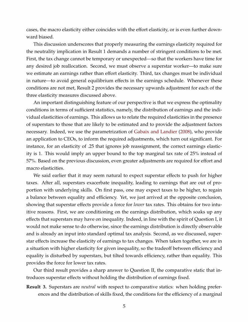
cases, the macro elasticity either coincides with the effort elasticity, or is even further down-ward biased.

This discussion underscores that properly measuring the earnings elasticity required forthe neutrality implication in Result 1 demands a number of stringent conditions to be met.First, the tax change cannot be temporary or unexpected—so that the workers have time forany desired job reallocation. Second, we must observe a superstar worker—to make surewe estimate an earnings rather than effort elasticity. Third, tax changes must be individualin nature—to avoid general equilibrium effects in the earnings schedule. Whenever theseconditions are not met, Result 2 provides the necessary upwards adjustment for each of thethree elasticity measures discussed above.

An important distinguishing feature of our perspective is that we express the optimalityconditions in terms of sufficient statistics, namely, the distribution of earnings and the indi-vidual elasticities of earnings. This allows us to relate the required elasticities in the presenceof superstars to those that are likely to be estimated and to provide the adjustment factorsnecessary. Indeed, we use the parametrization of Gabaix and Landier (2008), who providean application to CEOs, to inform the required adjustments, which turn out significant. Forinstance, for an elasticity of .25 that ignores job reassignment, the correct earnings elastic-ity is 1. This would imply an upper bound to the top marginal tax rate of 25% instead of57%. Based on the previous discussion, even greater adjustments are required for effort andmacro elasticities.

We said earlier that it may seem natural to expect superstar effects to push for highertaxes. After all, superstars exacerbate inequality, leading to earnings that are out of pro-portion with underlying skills. On first pass, one may expect taxes to be higher, to regaina balance between equality and efficiency. Yet, we just arrived at the opposite conclusion,showing that superstar effects provide a force for lower tax rates. This obtains for two intu-itive reasons. First, we are conditioning on the earnings distribution, which soaks up anyeffects that superstars may have on inequality. Indeed, in line with the spirit of Question I, itwould not make sense to do otherwise, since the earnings distribution is directly observableand is already an input into standard optimal tax analysis. Second, as we discussed, super-star effects increase the elasticity of earnings to tax changes. When taken together, we are ina situation with higher elasticity for given inequality, so the tradeoff between efficiency andequality is disturbed by superstars, but tilted towards efficiency, rather than equality. Thisprovides the force for lower tax rates.

Our third result provides a sharp answer to Question II, the comparative static that in-troduces superstar effects without holding the distribution of earnings fixed.

Result 3. Superstars are neutral with respect to comparative statics: when holding prefer-ences and the distribution of skills fixed, the conditions for the efficiency of a marginal

5

tax rate schedule do not depend on whether superstar effects are present.

This provides a very different neutrality result. Instead of holding the earnings distributionfixed, it considers a change in technology, such as the introduction of superstar effects, whichgenerally increases inequality. This result is based on the fact that the conditions for Paretoefficiency can be expressed in terms of the primitive distribution of skills and the elasticityof effort, determined by preferences only and invariant to the presence of superstar effects,unlike the elasticity of earnings.

This suggests that when superstars are introduced optimal tax rates remain unchanged.Indeed, this is the case in natural benchmark cases. The only caveat is that when performinga comparative static of this sort the allocation will generally change, even if taxes do not,and effort elasticities may depend on where they are evaluated. Likewise, for any givensocial welfare function, marginal social welfare weights may also be affected by where theyare evaluated. Nevertheless, when preferences have constant elasticity and when marginalsocial welfare weights are left unchanged, then one can conclude that marginal tax rates areunchanged. In particular, this is the case at the top of the distribution, when one applies azero weight at the top, e.g. utilitarian or Rawlsian social welfare functions.

How does this last neutrality result relate to our two previous results? Result 1 showsthat the distribution of earnings affects efficient tax schedules. Typically, the higher inequal-ity that comes with the introduction of superstar effects will justify higher tax rates. On theother hand, Result 2 shows that superstar effects increase the elasticity of earnings. Accord-ing to Result 3, these two opposing effects on optimal taxes precisely cancel out.

Related Literature. We build on the positive literature on assignment models that areable to generate superstar effects, surveyed in Sattinger (1993) and more recently Edmansand Gabaix (2015) and Garicano and Rossi-Hansberg (2015). This literature has been inter-ested in how these models can explain observed patterns of occupational choice and incomeinequality. Our contribution is to add a normative perspective, characterizing optimal re-distribution and taxation in a broad class of models used in the literature. Our baselinemodel is a general one-on-one assignment model between workers and jobs that captures,for example, Terviö (2008) and Gabaix and Landier (2008). Indeed, we inform our elas-ticity adjustments using the empirical results of Gabaix and Landier (2008), and provide afully specified parametric example that is able to match their evidence. We later extend theanalysis to other settings, such as the one-to-many span-of-control models developed by Lu-cas (1978) and Rosen (1982), as well as the knowledge-based hierarchy models in Garicano(2000) and Garicano and Rossi-Hansberg (2015).

Our paper incorporates a richer labor market into the canonical Mirrlees model. Thestandard Mirrlees model proceeds with the most basic of labor markets, where exogenous

6

wage differences simply reflect exogenous skill differences. In contrast, labor economistshave developed much richer general equilibrium models of the labor market. Much researchhas enriched the standard Mirrlees model in various of these directions, for example, byconsidering labor indivisibilities, human capital accumulation, uncertainty, or sorting acrossdifferent occupations, as in the Roy model, to name just a few.

Recent contributions focus on models with worker sorting across jobs and their generalequilibrium effects. In particular, Rothschild and Scheuer (2013) and Ales et al. (2014) showhow endogenous sectoral wages and assignments affect optimal income tax schedules. Inthese models, relative wages enter incentive constraints. The planner sets taxes with aneye towards influencing these relative wages so as to relax these constraints, generalizingthe insight from the two-type model by Stiglitz (1982). The same effect is featured in themodels by Scheuer (2014) and Ales et al. (2015), which focus on occupational choice betweenworkers and managers and the role of endogenous firm size. The latter paper also workswith a version of the span-of-control model of Lucas (1978) and Rosen (1982), as we do in oneof our extensions, although, as we point out, our adaptation is different in crucial aspects.

While the present paper is part of this greater agenda extending the standard optimal taxmodel to incorporate important features of real-world labor markets, it is also quite distinct.Crucially, we focus on superstar effects, which none of the above papers have considered. In-deed, in all these papers each individual faces a linear earnings schedule—whereas a convexschedule is often taken to be the defining characteristic of superstar phenomena. To isolatethe effect of superstars, we purposefully abstract from Stiglitz effects, the central focus ofthe above literature over the standard Mirrlees model. Moreover, although our model incor-porates a richer labor market and features an equilibrium-determined wage schedule, ourresults are not driven by general equilibrium effects from tax changes, as is the case withStiglitz effects. Indeed, Results 1 and 2 call for “partial equilibrium” earnings elasticitieswith respect to individual tax changes.

We also abstract from externalities and other sources of inefficiencies, such as unproduc-tive rent-seeking or positive spillovers from innovation. For example, some top incomesmay be the result of contest-like tournaments with winner-takes-all compensation (Roth-schild and Scheuer, 2014a). Likewise, some CEOs may capture the board, due to poor cor-porate governance, and set their own pay at excessive levels, effectively stealing from stock-holders (Piketty et al., 2014). On the other hand, some top earners, such as innovators, maybe unable to capture their entire marginal product. As this literature shows, such inefficien-cies call for Pigouvian adjustments to taxes, but these issues are, once again, conceptuallydistinct from superstar effects, which are our focus.

Perhaps equally importantly, we also take a fundamentally different approach in deriv-ing our results. The literature so far has characterized the effects of richer labor markets on

7

taxes by computing optimal taxes and comparing them to standard Mirrleesian ones. Thisinvolves fixing primitives, such as preference parameters and the skill distribution, and cal-ibrating technological parameters using data, e.g. occupational patterns or the firm sizedistribution. Instead, we take a “sufficient statistics” perspective, writing taxes directly interms of observable distributions and elasticities. We relate the relevant elasticities in thepresence of superstars to those that are likely to be estimated in standard settings. We canthen show how these elasticities are affected by the presence of superstar effects. The effectsof superstars on taxes work exclusively through the sufficient statistics.

This approach is inspired by Saez (2001), who expressed optimal tax formulas in termsof the income distribution and elasticities, and Werning (2007), who developed tests for thePareto efficiency of any given tax schedule in place as a function of these statistics. This test-ing approach is particularly useful to derive Results 1 and 2, because it allows us to hold theobserved earnings distribution fixed when characterizing the effects of superstars. In con-trast, computing optimal taxes for given redistributive motives requires taking into accountthat the equilibrium income distribution changes when varying taxes and technology, as wedo when deriving Result 3.

In parallel and independent work, Ales and Sleet (2015) pursue a more structural, quan-titative approach to optimal taxation in a similar assignment model. Their focus is on howthe social weight placed on profits affects the optimal top marginal tax rate. In some cases,they also observe a downward force on this tax rate, even though through a different chan-nel, adjusting the Pareto tail of the inferred skill distribution rather than earnings elasticities.Their goal of quantifying this force is an important complement to our qualitative analyticalresults.

The paper is organized as follows. Section 2 introduces our baseline model and Section3 sets up the planning problem for Pareto efficient taxes. Sections 4, 5 and 6 are devoted toResults 1, 2 and 3, respectively. Section 7 discusses extensions of our baseline model andSection 8 concludes. All proofs are relegated to an appendix.

2 Superstars in an Assignment Model

We first lay out our baseline model, based on a one-to-one assignment setting similar toTerviö (2008). Assignment models capture the essence of the superstar phenomena intro-duced by Rosen (1981).3 In Section 7, we discuss other settings, including first- and second-generation span-of-control models. All our results go through in these more general settings.

3Rosen (1981) considered a setting where agents choose the scale of their production subject to given costs.This model is close in spirit to the span-of-control models that we consider later.

8

2.1 Setup and Equilibrium

Our model blends the canonical Mirrlees model with an assignment model, by introducingan effort decision in the latter.

Preferences. There is a continuum of measure one of workers with different ability typesθ. The utility function for type θ is

U(c, y, θ),

where c is consumption and y denotes the effective units of labor supplied to the market,or ’effort’ for short. The latter is best interpreted as a catch-all for what a worker brings tothe table, including what a worker does while on the job, e.g. the hours and intensity oftheir work effort, as well as what they do before they even reach the job market to makethemselves more productive, e.g. their human capital investment. We assume standardconditions on the utility function, including differentiability with Uc > 0, Uy < 0 and thethe single-crossing property, which requires that the marginal rate of substitution

MRS(c, y, θ) ≡ −Uy(c, y, θ)

Uc(c, y, θ)

is decreasing in θ, so that more able agents (higher θ) find it less costly to provide y. Thecanonical case studied by Mirrlees (1971) assumes U(c, y, θ) = u(c, 1− y/θ) for some utilityfunction u over consumption and leisure.

Ability is distributed according to the cumulative distribution function F(θ) with densityf (θ) and support Θ.

Technology. There is a unit measure of firms indexed by x, distributed according to thecumulative distribution function G(x).4 There is a single final consumption good. Produc-tion of this final good takes place through one-to-one matching between individuals andfirms. If an individual that provides y units of effort is matched with a firm of type x, thenthe output of this match equals

A(x, y),

where the function A is non-negative, increasing, twice differentiable and strictly supermod-ular: Axy(x, y) > 0.

An allocation specifies c(θ), y(θ) and a measure-preserving assignment rule, mapping

4Without loss of generality, one may normalize the distribution of x to be uniform on [0, 1], so that x can beinterpreted as the quantiles of the distribution of some underlying firm characteristic.

9

worker θ to firm x = σ(θ).5 The resource constraint is then

ˆc(θ)dF(θ) ≤

ˆA(σ(θ), y(θ))dF(θ) + E, (1)

where E ∈ R is an endowment net of government consumption.Following Terviö (2008) and Gabaix and Landier (2008), an important benchmark is when

A is linear in y, so that A(x, y) = a(x)y. Indeed, when A can be expressed as a productA(x, y) = a(x)γ(y) one can always renormalize y so that γ(y) = y. Our examples fall intothis class.

Labor Markets. Individuals are paid according to a schedule W(y) that is endogenouslydetermined in equilibrium, but is taken as given by both individuals and firms.

Individuals choose effort y to maximize utility, taking as given the earnings schedule anda nonlinear tax schedule T(w) set by the government. They solve

maxc,y

U(c, y, θ) s.t. c = W(y)− T(W(y)). (2)

with solution c(θ), y(θ), which by single-crossing are nondecreasing functions of θ.Firm x maximizes profits, solving

maxy{A(x, y)−W(y)}. (3)

Denote the solution by Y(x), which is monotone by the supermodularity of A. The necessaryfirst-order condition is

Ay(x, y) = W ′(y). (4)

Because firms are in fixed supply, they will earn economic profits. We assume equal own-ership of firms across individuals. Alternatively, we may assume that firm profits accrue tothe government, either because the government owns all firms directly or because it fullytaxes their profits, as in Diamond and Mirrlees (1971). These standard assumptions allow usto sidestep distributional effects from firm ownership, which are not at the heart of the issueof superstar workers.6

5A measure-preserving transformation σ is such that µF(σ−1(X)) = µG(X) for any subset of firms X, where

σ−1(X) denotes the set of workers θ with σ(θ) ∈ X, and µF, µG are the measures induced by the cumulativedistributions F and G, respectively.

6Profits are possible because we have assumed a fixed distribution of firms. If instead we modeled endoge-nous entry of firms, this would dissipate ex ante or average profits, negating their distributional effects. Suchan extension would take us away from the standard existing assignment models and is beyond the scope ofthe present paper.

10

Positive Assortative Matching. As we have noted, on the worker side y and θ are posi-tively related, due to the single-crossing assumption. On the firm side x and y are positivelyrelated, due to supermodularity of A. Together, these two facts imply that there is also apositive relation between x and θ, given by an increasing assignment function σ(θ). Weincorporate this fact in the definition of an equilibrium below.

Equilibrium Definition. An equilibrium consists of a tax schedule T(w), an earnings sched-ule W(y), firms’ demands Y(x), workers’ consumption and effort c(θ), y(θ), and an increas-ing assignment function σ(θ) mapping workers to firms satisfying: (i) Y(x) solves (3) givenW(y); (ii) c(θ), y(θ) solve (2) given W(y) and T(w); (iii) goods market clearing: the resourceconstraint (1) holds with equality; and (iv) labor market clearing:

F(θ) = G(σ(θ)),

y(θ) = Y(σ(θ)).

The last condition (iv) ensures that the match between worker θ and firm x = σ(θ) isconsistent with their respective supply and demand choices, y(θ) = Y(σ(θ)), and that themeasure of firms demanding Y(x) or less, which equals G(x), coincides with the measure ofworkers supplying y(θ) or less, which equals F(θ). Equivalently, we can write the equalityof supply and demand for each skill level in differential form as f (θ) = g(σ(θ))σ′(θ). Thisis a common way of writing the market-clearing condition in hedonic markets.

By Walras’ law, the resource constraint implies that the government budget constraint

ˆT(W(y(θ)))dF(θ) + E + Π = 0

holds, where Π ≡´(A(x, Y(x))−W(Y(x)))dG(x) are aggregate profits.

2.2 Superstar Effects

Denoting by Γ(y) the inverse of y(θ), (4) becomes

W ′(y) = Ay(σ(Γ(y)), y). (5)

For a given effort schedule y(θ), this condition pins down the earnings schedule W(y) upto a constant.7 This well-known marginal condition, which obtains in a wide set of assign-

7In our model, with an equal number of firms and workers, this constant may not be uniquely determined.With more firms than workers, only the top firms are active and earn positive profits. The lowest active firmmakes zero profits, pinning down the constant. If A(0, 0) = 0, this implies W(0) = 0.

11

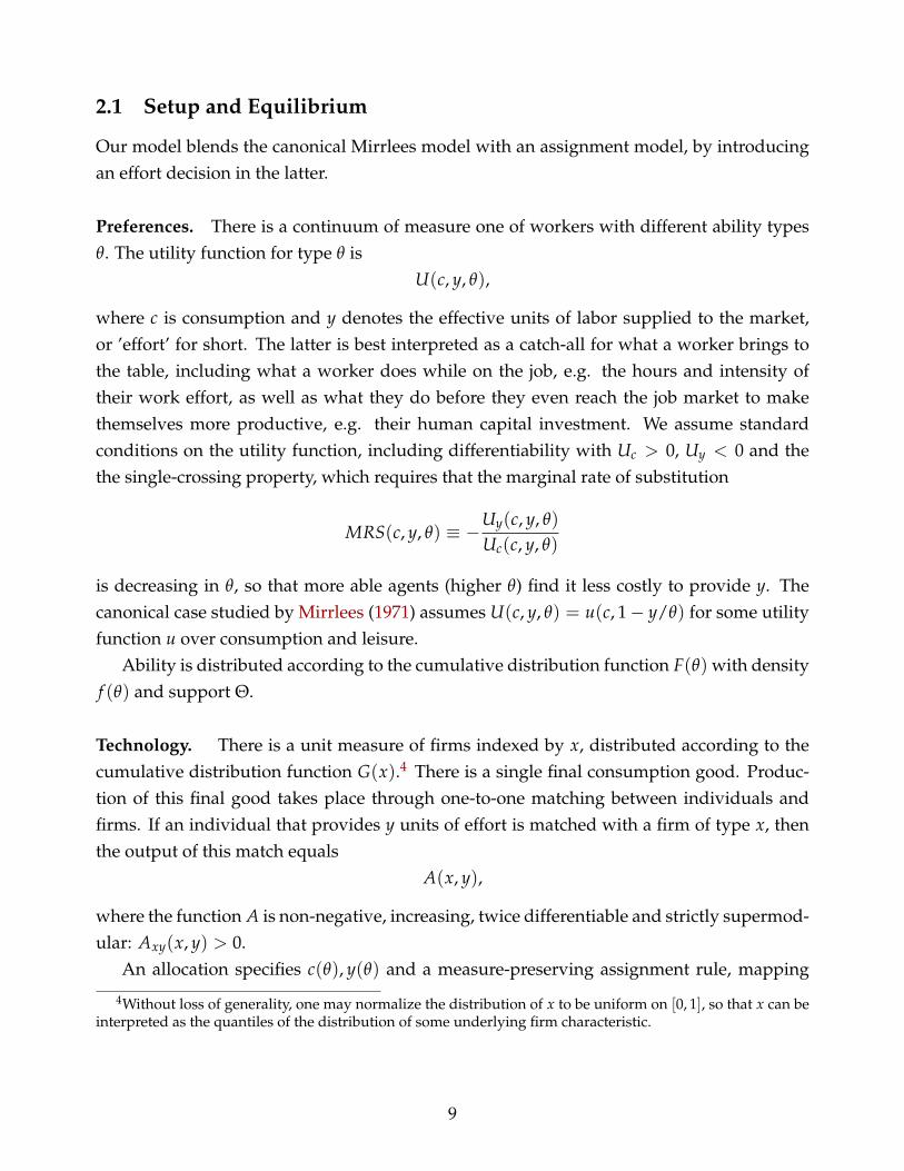
W(y)

U2

U3

U1

y

c

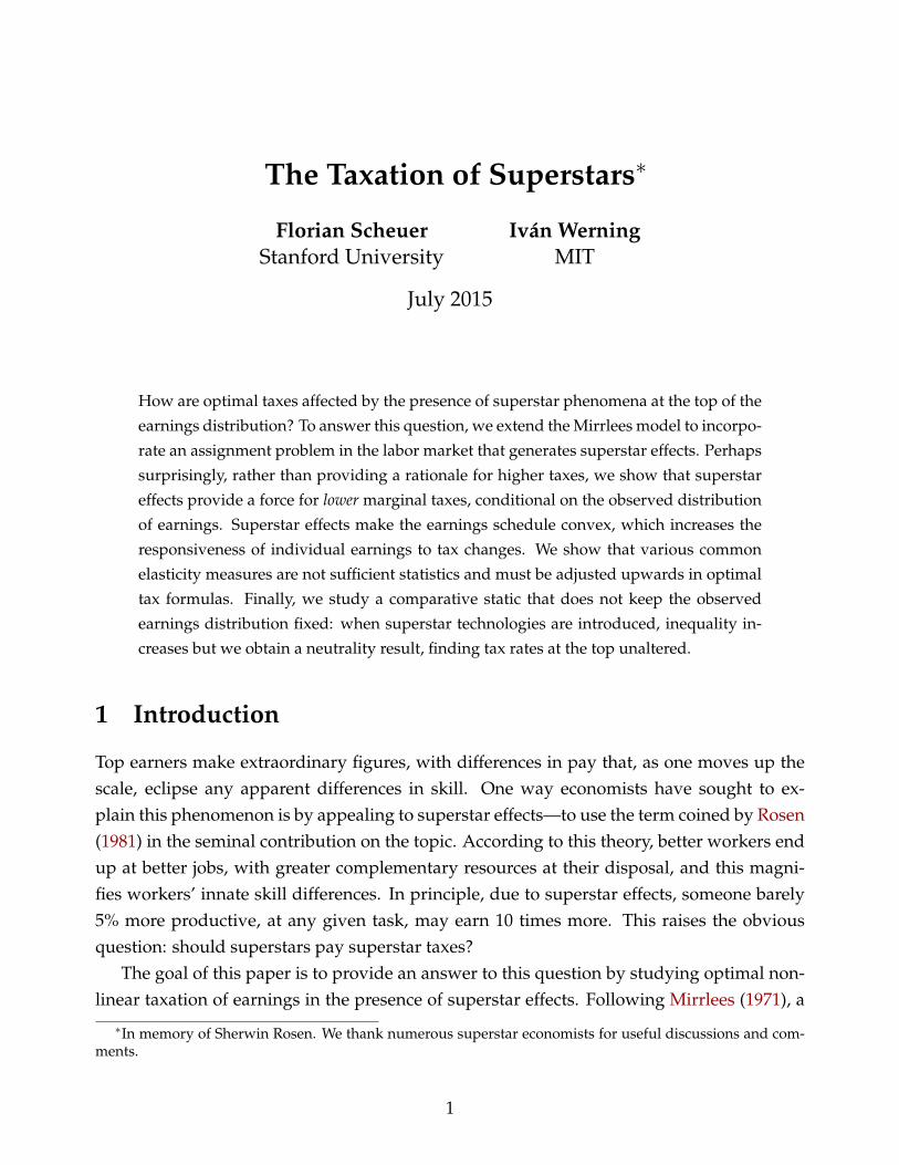
Figure 1: Convex equilibrium earnings schedule.

ment models, is fundamental to the superstar effects on the earnings schedule. To see this,differentiate to obtain

W ′′(y) = Ayθ(σ(Γ(y)), y) · σ′(Γ(y)) · Γ′(y) + Ayy(σ(Γ(y)), y). (6)

By supermodularity, the first term is positive, providing a force for the earnings schedule tobe convex in effort. When A is linear in y, then A(θ, y) = a(x)y for some increasing functiona and so W ′(y) = a(σ(Γ(y))) is increasing in y. In this case, output is linear in y at thefirm level, but earnings are convex, W ′′(y) > 0, as individuals with higher y get matched tohigher-x firms, which is reflected in the earnings schedule. This is illustrated in Figure 1.

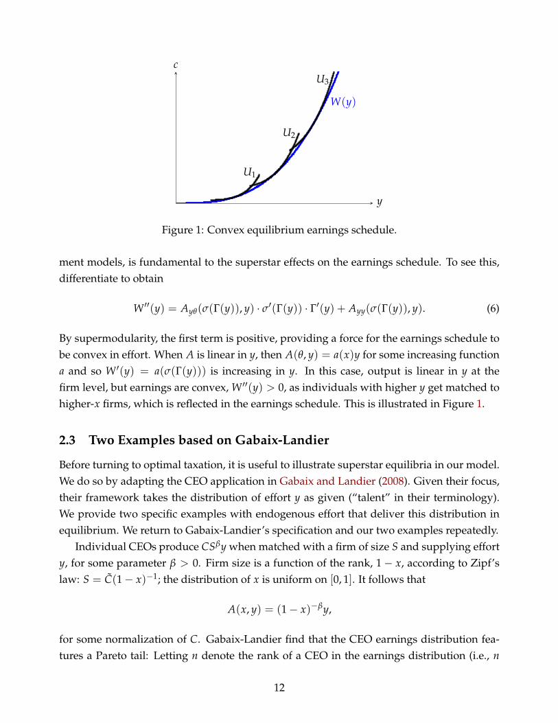
2.3 Two Examples based on Gabaix-Landier

Before turning to optimal taxation, it is useful to illustrate superstar equilibria in our model.We do so by adapting the CEO application in Gabaix and Landier (2008). Given their focus,their framework takes the distribution of effort y as given (“talent” in their terminology).We provide two specific examples with endogenous effort that deliver this distribution inequilibrium. We return to Gabaix-Landier’s specification and our two examples repeatedly.

Individual CEOs produce CSβy when matched with a firm of size S and supplying efforty, for some parameter β > 0. Firm size is a function of the rank, 1− x, according to Zipf’slaw: S = C(1− x)−1; the distribution of x is uniform on [0, 1]. It follows that

A(x, y) = (1− x)−βy,

for some normalization of C. Gabaix-Landier find that the CEO earnings distribution fea-tures a Pareto tail: Letting n denote the rank of a CEO in the earnings distribution (i.e., n

12

equals 1 minus the cdf), we have near the top8

w(n) = κn−1/ρ, (7)

where ρ is the Pareto parameter.We can restate problem (3) for firm x as maximizing (1− x)−βy(n)− w(n), implying

y′(n) = nβw′(n) = −κ

ρnβ− 1

ρ−1,

where we used that in equilibrium n = 1− x. For some constant of integration b,

y(n) = b− κ

βρ− 1nβ− 1

ρ . (8)

When βρ > 1, effort is bounded above by b.9 Otherwise, effort is unbounded above. Com-bining equations (7) with (8) gives the increasing and convex earnings schedule

W(y) =

κ (b− y)−1

βρ−1 if βρ > 1

κ (y− b)1

1−βρ if βρ < 1(9)

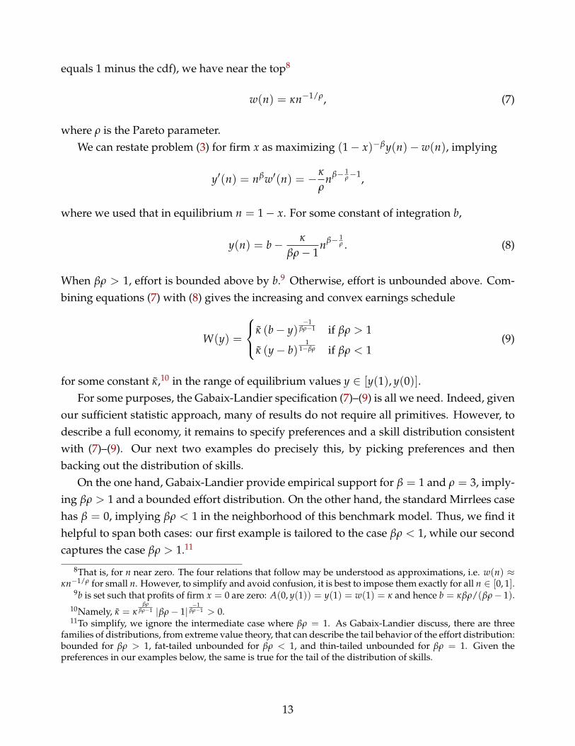
for some constant κ,10 in the range of equilibrium values y ∈ [y(1), y(0)].For some purposes, the Gabaix-Landier specification (7)–(9) is all we need. Indeed, given

our sufficient statistic approach, many of results do not require all primitives. However, todescribe a full economy, it remains to specify preferences and a skill distribution consistentwith (7)–(9). Our next two examples do precisely this, by picking preferences and thenbacking out the distribution of skills.

On the one hand, Gabaix-Landier provide empirical support for β = 1 and ρ = 3, imply-ing βρ > 1 and a bounded effort distribution. On the other hand, the standard Mirrlees casehas β = 0, implying βρ < 1 in the neighborhood of this benchmark model. Thus, we find ithelpful to span both cases: our first example is tailored to the case βρ < 1, while our secondcaptures the case βρ > 1.11

8That is, for n near zero. The four relations that follow may be understood as approximations, i.e. w(n) ≈κn−1/ρ for small n. However, to simplify and avoid confusion, it is best to impose them exactly for all n ∈ [0, 1].

9b is set such that profits of firm x = 0 are zero: A(0, y(1)) = y(1) = w(1) = κ and hence b = κβρ/(βρ− 1).10Namely, κ = κ

βρβρ−1 |βρ− 1|

−1βρ−1 > 0.

11To simplify, we ignore the intermediate case where βρ = 1. As Gabaix-Landier discuss, there are threefamilies of distributions, from extreme value theory, that can describe the tail behavior of the effort distribution:bounded for βρ > 1, fat-tailed unbounded for βρ < 1, and thin-tailed unbounded for βρ = 1. Given thepreferences in our examples below, the same is true for the tail of the distribution of skills.

13

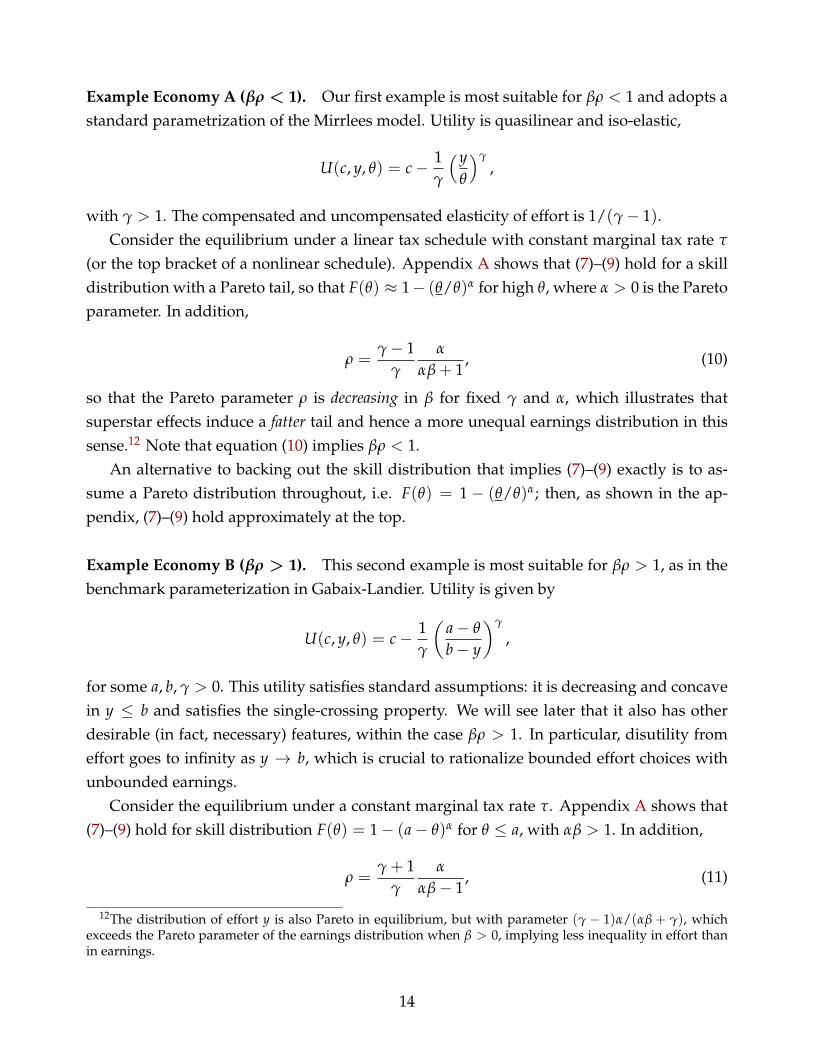
Example Economy A (βρ < 1). Our first example is most suitable for βρ < 1 and adopts astandard parametrization of the Mirrlees model. Utility is quasilinear and iso-elastic,

U(c, y, θ) = c− 1γ

(yθ

)γ,

with γ > 1. The compensated and uncompensated elasticity of effort is 1/(γ− 1).Consider the equilibrium under a linear tax schedule with constant marginal tax rate τ

(or the top bracket of a nonlinear schedule). Appendix A shows that (7)–(9) hold for a skilldistribution with a Pareto tail, so that F(θ) ≈ 1− (θ/θ)α for high θ, where α > 0 is the Paretoparameter. In addition,

ρ =γ− 1

γ

α

αβ + 1, (10)

so that the Pareto parameter ρ is decreasing in β for fixed γ and α, which illustrates thatsuperstar effects induce a fatter tail and hence a more unequal earnings distribution in thissense.12 Note that equation (10) implies βρ < 1.

An alternative to backing out the skill distribution that implies (7)–(9) exactly is to as-sume a Pareto distribution throughout, i.e. F(θ) = 1− (θ/θ)α; then, as shown in the ap-pendix, (7)–(9) hold approximately at the top.

Example Economy B (βρ > 1). This second example is most suitable for βρ > 1, as in thebenchmark parameterization in Gabaix-Landier. Utility is given by

U(c, y, θ) = c− 1γ

(a− θ

b− y

)γ

,

for some a, b, γ > 0. This utility satisfies standard assumptions: it is decreasing and concavein y ≤ b and satisfies the single-crossing property. We will see later that it also has otherdesirable (in fact, necessary) features, within the case βρ > 1. In particular, disutility fromeffort goes to infinity as y → b, which is crucial to rationalize bounded effort choices withunbounded earnings.

Consider the equilibrium under a constant marginal tax rate τ. Appendix A shows that(7)–(9) hold for skill distribution F(θ) = 1− (a− θ)α for θ ≤ a, with αβ > 1. In addition,

ρ =γ + 1

γ

α

αβ− 1, (11)

12The distribution of effort y is also Pareto in equilibrium, but with parameter (γ − 1)α/(αβ + γ), whichexceeds the Pareto parameter of the earnings distribution when β > 0, implying less inequality in effort thanin earnings.

14

which is decreasing in β, so that earnings inequality is again increasing in β. Note that (11)implies βρ > 1. In particular, we can always find α and γ so that ρ = 3 and β = 1, consistentwith Gabaix-Landier’s favored parameterization.

3 Efficient Taxes and Planning Problem

We now turn to the normative study of optimal or efficient taxes T. We first develop aplanning problem that can be used to characterize efficient taxes. Our results in later sectionsexploit the optimality conditions of this planning problem.

3.1 Planning Problem

We first establish a connection between incentive compatible allocations and allocations thatare part of an equilibrium with some taxes T. This implementation result allows us to for-mulate a planning problem in terms of allocations directly.

Incentive Compatibility and Tax Implementation. For any allocation (c(θ), y(θ)), definethe utility assignment

V(θ) = U(c(θ), y(θ), θ). (12)

An allocation is incentive compatible when

V(θ) = maxθ′

U(c(θ′), y(θ′), θ) ∀θ. (13)

The following lemma relates equilibria with taxes and incentive compatible allocations.

Lemma 1. An allocation (c(θ), y(θ), σ(θ)) is part of an equilibrium for some tax schedule T(w) ifand only if it is resource feasible (1), incentive compatible (12)–(13) and σ(θ) = G−1(F(θ)).

The proof is contained in Appendix B.1. The key to the ’only if’ part is that, although theearnings schedule is determined by the labor market and the government cannot observe ortax effort y directly, it can, for any monotone earnings schedule W(y), create incentives usingthe tax schedule to tailor consumption W(y) − T(W(y)) at will, subject only to incentivecompatibility.

By single-crossing, the global incentive constraints (12) and (13) are equivalent to thelocal constraints

V′(θ) = Uθ(c(θ), y(θ), θ) ∀θ (14)

and the requirementy(θ) is non-decreasing. (15)

15

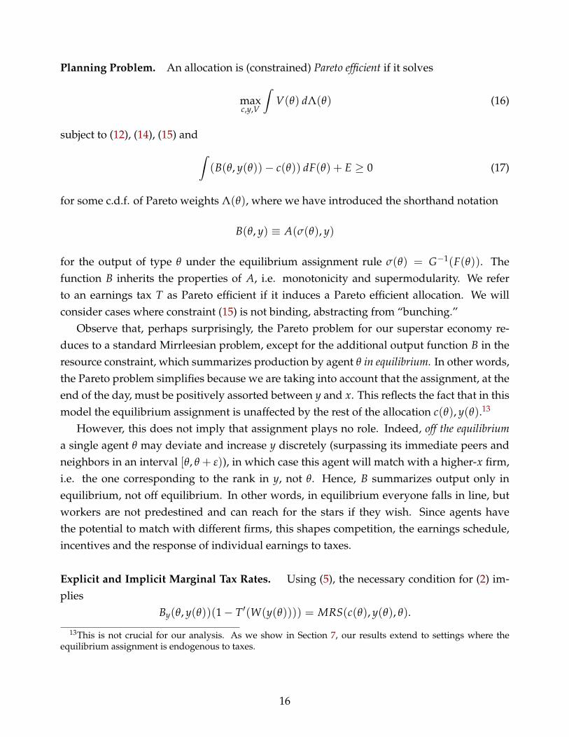
Planning Problem. An allocation is (constrained) Pareto efficient if it solves

maxc,y,V

ˆV(θ) dΛ(θ) (16)

subject to (12), (14), (15) and

ˆ(B(θ, y(θ))− c(θ)) dF(θ) + E ≥ 0 (17)

for some c.d.f. of Pareto weights Λ(θ), where we have introduced the shorthand notation

B(θ, y) ≡ A(σ(θ), y)

for the output of type θ under the equilibrium assignment rule σ(θ) = G−1(F(θ)). Thefunction B inherits the properties of A, i.e. monotonicity and supermodularity. We referto an earnings tax T as Pareto efficient if it induces a Pareto efficient allocation. We willconsider cases where constraint (15) is not binding, abstracting from “bunching.”

Observe that, perhaps surprisingly, the Pareto problem for our superstar economy re-duces to a standard Mirrleesian problem, except for the additional output function B in theresource constraint, which summarizes production by agent θ in equilibrium. In other words,the Pareto problem simplifies because we are taking into account that the assignment, at theend of the day, must be positively assorted between y and x. This reflects the fact that in thismodel the equilibrium assignment is unaffected by the rest of the allocation c(θ), y(θ).13

However, this does not imply that assignment plays no role. Indeed, off the equilibriuma single agent θ may deviate and increase y discretely (surpassing its immediate peers andneighbors in an interval [θ, θ + ε)), in which case this agent will match with a higher-x firm,i.e. the one corresponding to the rank in y, not θ. Hence, B summarizes output only inequilibrium, not off equilibrium. In other words, in equilibrium everyone falls in line, butworkers are not predestined and can reach for the stars if they wish. Since agents havethe potential to match with different firms, this shapes competition, the earnings schedule,incentives and the response of individual earnings to taxes.

Explicit and Implicit Marginal Tax Rates. Using (5), the necessary condition for (2) im-plies

By(θ, y(θ))(1− T′(W(y(θ)))) = MRS(c(θ), y(θ), θ).

13This is not crucial for our analysis. As we show in Section 7, our results extend to settings where theequilibrium assignment is endogenous to taxes.

16

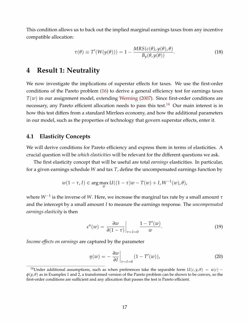
This condition allows us to back out the implied marginal earnings taxes from any incentivecompatible allocation:

τ(θ) ≡ T′(W(y(θ))) = 1− MRS(c(θ), y(θ), θ)

By(θ, y(θ)). (18)

4 Result 1: Neutrality

We now investigate the implications of superstar effects for taxes. We use the first-orderconditions of the Pareto problem (16) to derive a general efficiency test for earnings taxesT(w) in our assignment model, extending Werning (2007). Since first-order conditions arenecessary, any Pareto efficient allocation needs to pass this test.14 Our main interest is inhow this test differs from a standard Mirrlees economy, and how the additional parametersin our model, such as the properties of technology that govern superstar effects, enter it.

4.1 Elasticity Concepts

We will derive conditions for Pareto efficiency and express them in terms of elasticities. Acrucial question will be which elasticities will be relevant for the different questions we ask.

The first elasticity concept that will be useful are total earnings elasticities. In particular,for a given earnings schedule W and tax T, define the uncompensated earnings function by

w(1− τ, I) ∈ arg maxw

U((1− τ)w− T(w) + I, W−1(w), θ),

where W−1 is the inverse of W. Here, we increase the marginal tax rate by a small amount τ

and the intercept by a small amount I to measure the earnings response. The uncompensatedearnings elasticity is then

εu(w) =∂w

∂(1− τ)

∣∣∣∣τ=I=0

1− T′(w)

w. (19)

Income effects on earnings are captured by the parameter

η(w) = − ∂w∂I

∣∣∣∣τ=I=0

(1− T′(w)), (20)

14Under additional assumptions, such as when preferences take the separable form U(c, y, θ) = u(c) −φ(y, θ) as in Examples 1 and 2, a transformed version of the Pareto problem can be shown to be convex, so thefirst-order conditions are sufficient and any allocation that passes the test is Pareto efficient.

17

and the compensated earnings elasticity leaves utility constant with

εc(w) = εu(w) + η(w), (21)

by the Slutsky equation.Three observations are in order. First, these are elasticities for earnings, so they take into

account the shape of the equilibrium earnings schedule W(y).15 Second, these elasticitiesare micro, partial equilibrium elasticities that hold the earnings schedule W(y) fixed. Atthe macro level, of course, general equilibrium effects imply that the earnings schedule isendogenous to the tax schedule. Third, these elasticities measure earnings responses undera given (nonlinear) tax schedule T in place. We will return to a detailed discussion of theseelasticities in Section 5 and contrast them with other elasticity concepts.

4.2 An Efficiency Test

We denote the equilibrium earnings distribution under a given tax schedule by H(w) withcorresponding density h(w). This allows us to state our first result.

Proposition 1. Any Pareto efficient earnings tax T(w) satisfies

T′(w)

1− T′(w)εc(w)

ρ(w)−d log

(T′(w)

1−T′(w)εc(w)

)d log w

− η(w)

εc(w)

≤ 1 (22)

at all equilibrium earnings levels w, where

ρ(w) ≡ −(

1 +d log h(w)

d log w

)is the local Pareto parameter of the earnings distribution.

Proposition 1, proved in Appendix B.2, reveals three, perhaps surprising, insights. First,for a given tax schedule T, the observed distribution of earnings h as well as the earningselasticities εc and εu (which imply η = εc − εu) are sufficient to evaluate the efficiency test.Conditional on these sufficient statistics, no further knowledge about the structural param-eters of the economy and the superstar technology are required. Among these sufficientstatistics, the distribution of earnings is directly observable; in principle, the elasticity ofearnings may be estimated, although, as we argue below, identifying it is challenging.

15This is in contrast to pure effort elasticities. Our earnings elasticities are therefore more closely related tothe empirical literature on taxable income elasticities than, for instance, traditional labor supply elasticities asmeasured by hours. Keane (2011), Chetty (2012), Keane and Rogerson (2012) and Saez et al. (2012) providerecent surveys. See Section 5 for more details.

18

Second, condition (22) is the same as in a standard Mirrlees model with linear production(see Werning, 2007). Of course, as is common with sufficient statistics, the earnings distribu-tion and elasticities are endogenous in general, and we will later show how they are affectedby superstar effects. Nonetheless, once we have measures for them from the equilibriumunder a given tax schedule, the formula is completely independent of whether there aresuperstars or not. In this sense, superstars are neutral conditional on the sufficient statistics.

Third, the relevant elasticities turn out to be precisely the earnings elasticities defined inthe previous subsection, taking the equilibrium earnings schedule W(y) and the tax T asgiven. Indeed, this is the key channel through which superstar effects enter the test formula.Therefore, a crucial question that we address in the next section is how superstar effectsaffect these earnings elasticities and how they may compare with the elasticities typicallyestimated in the empirical literature.

Intuition. Condition (22) provides an upper bound for Pareto efficient marginal tax ratesat w. The intuition can be grasped by imagining a reduction in taxes locally around a givenearnings level w, and checking whether the induced behavioral responses lead to an increasein tax revenue; if they do, there is a local Laffer effect, and the original tax schedule cannothave been Pareto efficient. As in Werning (2007), this can be done by comparing the (posi-tive) effect on revenue of those who initially earn less than w and thus increase their earningsto benefit from the tax reduction at w, and the (negative) effect of those initially above w whoreduce their earnings.

If the earnings density falls quickly at w (the local Pareto parameter is positive and large)the first effect is likely to outweigh the second, and we are more likely to reject Pareto ef-ficiency based on (22). Similarly to a high earnings elasticity (in front of the brackets), thispushes for a lower upper bound on the marginal tax at w. On the other hand, if the tax sched-ule is very progressive (T′ increases quickly) or the earnings elasticity increases quickly atw, then the second term in brackets is negative and large in absolute value, and we losemore revenue from the second group than we gain from the first. Hence, a local Laffer effectbecomes less likely, allowing for higher taxes. The same is true if income effects are large (soη is positive and large) for the reasons emphasized in Saez (2001).

Rawlsian Optimum. In fact, there is a tight connection between the efficiency test and theoptimal tax schedule under a Rawlsian criterion, which effectively only puts positive Paretoweight on the lowest θ-type in (16). The optimum then sets the tax rate at the maximal levelconsistent with (22). This leads to the following corollary.

19

Corollary 1. The optimal Rawlsian tax schedule satisfies

T′(w)

1− T′(w)=

1εc(w)wh(w)

ˆ ∞

wexp

[ˆ s

w

η(t)εc(t)

dtt

]dH(s) ∀w.

This corresponds to the integral version of (22) evaluated as an equality everywhere.

The role of earnings elasticities and the earnings distribution. We illustrate the useful-ness of Proposition 1 in the simpler case when there are no income effects on earnings, so εc

and εu coincide, and the tax schedule is locally linear at w, with marginal tax rate τ. Hence,(22) reduces to

τ

1− τε(w)

[ρ(w)− d log ε(w)

d log w

]≤ 1. (23)

The upper bound on τ now only depends on the shape of the equilibrium earnings distribu-tion h(w) (as captured by the local Pareto parameter ρ(w)) and the earnings elasticity ε(w)

(and its change) at w. The same holds, by Corollary 1, for the optimal Rawlsian tax schedule,which now reduces to

T′(w)

1− T′(w)=

(ε(w)

wh(w)

1− H(w)

)−1

∀w, (24)

the inverse of the earnings elasticity times a measure of the tail thickness of the earningsdistribution.16

This motivates two questions that we will investigate in the following. First, supposewe have a tax T in place and observe the empirical earnings distribution in the resultingequilibrium. Given this earnings distribution, does the presence of superstar effects makeit more or less likely that the efficiency test (23) is passed, i.e., does it push for lower orhigher taxes? We see that this crucially depends on how superstars affect earnings elastic-ities, which we will explore in detail in the next Section 5. Second, for given fundamentals(in particular a given skill distribution and preferences), how do superstar effects changethe set of Pareto efficient taxes? For instance, how do superstars affect revenue-maximizingmarginal tax rates through their effect, in view of (24), on both the earnings distribution andearnings elasticities? We turn to this comparative static exercise in Section 6.

16In the special case where H is a Pareto distribution with parameter ρ, this measure equals the Paretoparameter: wh(w)

1−H(w)= −

(1 + d log h(w)

d log w

)= ρ. This also is true at the top for any distribution: if either measures,

wh(w)1−H(w)

or ρ(w) = −(

1 + d log h(w)d log w

), converge as w→ ∞ then they must coincide.

20

5 Result 2: Superstars and Earnings Elasticities

In the previous section, we showed that the test for the efficiency of a given tax schedule onlydepends on the (directly observable) earnings distribution as well as the earnings elasticitiesof superstars under this tax. In this section, we explain how to apply the test in practice ifavailable estimates of earnings elasticities in fact do not appropriately account for superstarphenomena. A closely related question we also address is how the efficiency test wouldchange if we believed that the observed earnings distribution was generated by a standardeconomy without superstars.

5.1 Estimated versus Required Elasticities

To apply the efficiency test, we need the correct earnings elasticities for superstars, as definedin Section 4.1. Suppose, however, that the empirical estimates of earnings elasticities wehave access to do not properly capture superstar effects. This could be for the followingreasons:

1. The estimates measure fixed-assignment elasticities, where individuals are unable toswitch matches in response to tax changes, but only vary their effort at their currentmatch. This is likely to be the case if the estimates are based on temporary and/orunexpected tax changes.

2. The elasticities are estimated based on samples of non-superstar individuals. For ex-ample, the estimates could come from individuals lower in the earnings distribution,where superstar effects simply are not present. Or even if they are based on samplesof high-income individuals, they could be from settings where superstar phenomenaonly play a limited role.

3. The estimates are macro elasticities, which measure earnings responses to tax changesincluding the general equilibrium effects on the entire earnings schedule W(y). Forinstance, this is the case whenever identification comes from large tax reforms withaggregate effects. These elasticities are not the required ones, because they account forchanges in the equilibrium earnings schedule in response to tax changes, instead ofholding W(y) fixed when measuring earnings responses.

In the next 3 subsections, we address these scenarios and show in each case how the esti-mated elasticities need to be adjusted in order to use them for the efficiency test.

21

5.2 Fixed-Assignment Elasticities

Consider the equilibrium under a given earnings tax T in place, with equilibrium earn-ings schedule W(y) and effort allocation y(θ). Pick an individual in this equilibrium withobserved earnings w0. We can back out this individual’s effort y0 = W−1(w0) and typeθ0 = Γ(y0). We can always write earnings as follows:

w0 = B(θ0, y0)− π(θ0),

i.e. as the difference between output and profits at the firm type θ0 is matched with.

Fixed-Assignment Earnings Schedules. To formalize the idea that the empirically es-timated elasticity of earnings at w0 captures behavioral responses under fixed assignmentonly, suppose that it is based on the following “non-superstar” earnings schedule

W0(y) = B(θ0, y)− π(θ0). (25)

W0 is the schedule that results from letting the individual with earnings w0 stay at the firmshe is assigned to in the superstar equilibrium. In fact, by (5),

W ′0(y0) = By(θ0, y0) = W ′(y0),

so W0(y) both coincides with and is tangent to the original superstar earnings schedule W(y)at w0, but otherwise follows the shape of the output function B(θ0, y) of the firm that type θ0

is matched with in equilibrium. Hence, this is precisely the relationship between effort andearnings that this individual would perceive when confined to staying with the same firm.

In the case where A is linear in y (and hence B(θ, y) = b(θ)y for some increasing functionb), the interpretation is particularly simple: then W0(y) is linear, and given by the line that istangent to W(y) at w0:

W0(y) = w0 + b(θ0)(y− y0) = w0 + W ′(y0)(y− y0).

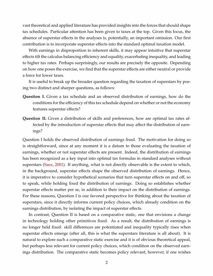
In this sense, W0 neatly captures the absence of superstar effects, as it ignores the convexity ofthe true earnings schedule W and instead describes a standard, linear relationship betweenearnings and effort, as illustrated in Figure 2.

Adjusting Fixed-Assignment Elasticities. Denote the resulting earnings elasticities andincome effect by εu(w0), η(w0) and εc(w0), defined as in (19)–(21) when replacing W byW0. The following result shows how they differ from the elasticity terms required for the

22

W(y)

W0(y)

y0

w0

y

c

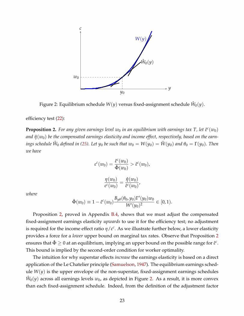
Figure 2: Equilibrium schedule W(y) versus fixed-assignment schedule W0(y).

efficiency test (22):

Proposition 2. For any given earnings level w0 in an equilibrium with earnings tax T, let εc(w0)

and η(w0) be the compensated earnings elasticity and income effect, respectively, based on the earn-ings schedule W0 defined in (25). Let y0 be such that w0 = W(y0) = W(y0) and θ0 = Γ(y0). Thenwe have

εc(w0) =εc(w0)

Φ(w0)> εc(w0),

η(w0)

εc(w0)=

η(w0)

εc(w0),

where

Φ(w0) ≡ 1− εc(w0)Byθ(θ0, y0)Γ′(y0)w0

W ′(y0)2 ∈ [0, 1).

Proposition 2, proved in Appendix B.4, shows that we must adjust the compensatedfixed-assignment earnings elasticity upwards to use it for the efficiency test; no adjustmentis required for the income effect ratio η/εc. As we illustrate further below, a lower elasticityprovides a force for a lower upper bound on marginal tax rates. Observe that Proposition 2ensures that Φ ≥ 0 at an equilibrium, implying an upper bound on the possible range for εc.This bound is implied by the second-order condition for worker optimality.

The intuition for why superstar effects increase the earnings elasticity is based on a directapplication of the Le Chatelier principle (Samuelson, 1947). The equilibrium earnings sched-ule W(y) is the upper envelope of the non-superstar, fixed-assignment earnings schedulesW0(y) across all earnings levels w0, as depicted in Figure 2. As a result, it is more convexthan each fixed-assignment schedule. Indeed, from the definition of the adjustment factor

23

U

W(y)

y

c

U

W(y)

y

c

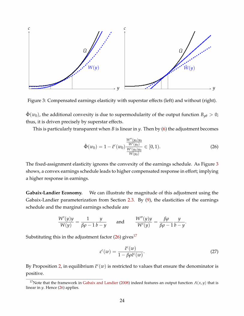
Figure 3: Compensated earnings elasticity with superstar effects (left) and without (right).

Φ(w0), the additional convexity is due to supermodularity of the output function Byθ > 0;thus, it is driven precisely by superstar effects.

This is particularly transparent when B is linear in y. Then by (6) the adjustment becomes

Φ(w0) = 1− εc(w0)

W ′′(y0)y0W ′(y0)

W ′(y0)y0W(y0)

∈ [0, 1). (26)

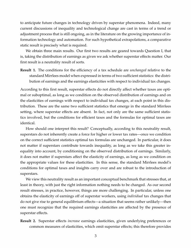
The fixed-assignment elasticity ignores the convexity of the earnings schedule. As Figure 3shows, a convex earnings schedule leads to higher compensated response in effort; implyinga higher response in earnings.

Gabaix-Landier Economy. We can illustrate the magnitude of this adjustment using theGabaix-Landier parameterization from Section 2.3. By (9), the elasticities of the earningsschedule and the marginal earnings schedule are

W ′(y)yW(y)

=1

βρ− 1y

b− yand

W ′′(y)yW ′(y)

=βρ

βρ− 1y

b− y.

Substituting this in the adjustment factor (26) gives17

εc(w) =εc(w)

1− βρεc(w). (27)

By Proposition 2, in equilibrium εc(w) is restricted to values that ensure the denominator ispositive.

17Note that the framework in Gabaix and Landier (2008) indeed features an output function A(x, y) that islinear in y. Hence (26) applies.

24

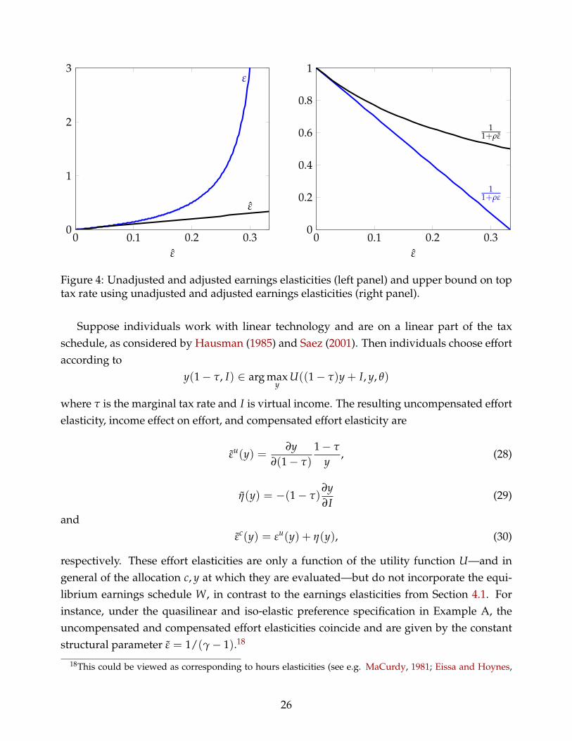
As an illustration, recall that Gabaix-Landier’s preferred parameterization has β = 1 andρ = 3; this requires εc ≤ 1

βρ = 13 to be consistent with an equilibrium. Equation (27) provides

potentially drastic upward adjustments in fixed-assignment elasticities. For instance, if εc =

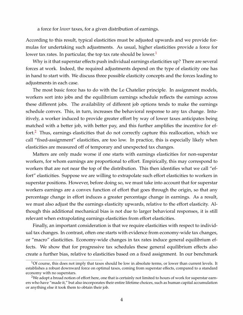
1/4, then the correct earnings elasticity is in fact εc = 1. The left panel of Figure 4 displaysεc as a function of εc ∈ [0, 1/3). The adjustment becomes infinite as εc → 1/3.

Tax Implications of Superstar Earnings Elasticities. In general, the test condition inProposition 1 not only depends on the level of the earnings elasticity, but also on how itchanges along the earnings distribution, as captured by the term d log εc(w)/d log w in (22).We therefore obtain particularly clean results in the important case where both marginal taxrates and elasticities are locally constant, such as in the top bracket of earnings:

Corollary 2. Suppose that, as w→ ∞, T′(w), ρ(w), εc(w) and η(w) all converge asymptotically tothe constants τ, ρ, εc and η, respectively. Suppose the same holds for the fixed-assignment elasticitiesεc(w)→ εc, η(w)→ η. Then (22) implies

τ

1− τ≤ 1

εc (ρ− η/εc)≤ 1

εc (ρ− η/εc).

Using the non-superstar elasticities delivers a less stringent upper bound to top marginaltax rates. Conversely, realizing that the earnings distribution is in fact the result of superstareffects pushes for a more stringent, lower upper bound to the top marginal tax rate. Alter-natively, this provides a comparison of the predictions for optimal taxation of a superstareconomy relative to a standard Mirrlees economy.

For the case of no income effects and using the Gabaix-Landier parameterization, theupper bound to the top marginal tax rate can be written as

τ ≤ 11 + ρε

=1

1 + ρ ε1−βρε

.

For instance, based on the Gabaix-Landier numbers β = 1 and ρ = 3, if ε = 1/4, thenτ ≤ 25%. Erroneously using the unadjusted ε instead of ε, one would have concluded thatτ ≤ 57%. The right panel in Figure 4 compares the correct upper bound to the unadjustedone as a function of the elasticity ε ∈ [0, 1/3).

5.3 Effort Elasticities

We now turn to the second scenario, where the estimated elasticities are effort elasticities,estimated in a Mirrleesian setting without superstar effects, where earnings simply equaleffort. The question is whether we can extrapolate these standard elasticities to superstars.

25

0 0.1 0.2 0.30

1

2

3ε

ε

ε

0 0.1 0.2 0.30

0.2

0.4

0.6

0.8

1

11+ρε

11+ρε

ε

Figure 4: Unadjusted and adjusted earnings elasticities (left panel) and upper bound on toptax rate using unadjusted and adjusted earnings elasticities (right panel).

Suppose individuals work with linear technology and are on a linear part of the taxschedule, as considered by Hausman (1985) and Saez (2001). Then individuals choose effortaccording to

y(1− τ, I) ∈ arg maxy

U((1− τ)y + I, y, θ)

where τ is the marginal tax rate and I is virtual income. The resulting uncompensated effortelasticity, income effect on effort, and compensated effort elasticity are

εu(y) =∂y

∂(1− τ)

1− τ

y, (28)

η(y) = −(1− τ)∂y∂I

(29)

andεc(y) = εu(y) + η(y), (30)

respectively. These effort elasticities are only a function of the utility function U—and ingeneral of the allocation c, y at which they are evaluated—but do not incorporate the equi-librium earnings schedule W, in contrast to the earnings elasticities from Section 4.1. Forinstance, under the quasilinear and iso-elastic preference specification in Example A, theuncompensated and compensated effort elasticities coincide and are given by the constantstructural parameter ε = 1/(γ− 1).18

18This could be viewed as corresponding to hours elasticities (see e.g. MaCurdy, 1981; Eissa and Hoynes,

26

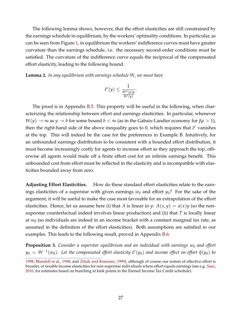
The following lemma shows, however, that the effort elasticities are still constrained bythe earnings schedule in equilibrium, by the workers’ optimality conditions. In particular, ascan be seen from Figure 1, in equilibrium the workers’ indifference curves must have greatercurvature than the earnings schedule, i.e. the necessary second-order conditions must besatisfied. The curvature of the indifference curve equals the reciprocal of the compensatedeffort elasticity, leading to the following bound.

Lemma 2. In any equilibrium with earnings schedule W, we must have

εc(y) ≤ 1W ′′(y)yW ′(y)

.

The proof is in Appendix B.5. This property will be useful in the following, when char-acterizing the relationship between effort and earnings elasticities. In particular, wheneverW(y)→ ∞ as y→ b for some bound b < ∞ (as in the Gabaix-Landier economy for βρ > 1),then the right-hand side of the above inequality goes to 0, which requires that εc vanishesat the top. This will indeed be the case for the preferences in Example B. Intuitively, foran unbounded earnings distribution to be consistent with a bounded effort distribution, itmust become increasingly costly for agents to increase effort as they approach the top, oth-erwise all agents would trade off a finite effort cost for an infinite earnings benefit. Thisunbounded cost from effort must be reflected in the elasticity and is incompatible with elas-ticities bounded away from zero.

Adjusting Effort Elasticities. How do these standard effort elasticities relate to the earn-ings elasticities of a superstar with given earnings w0 and effort y0? For the sake of theargument, it will be useful to make the case most favorable for an extrapolation of the effortelasticities. Hence, let us assume here (i) that A is linear in y: A(x, y) = a(x)y (so the non-superstar counterfactual indeed involves linear production) and (ii) that T is locally linearat w0 (so individuals are indeed in an income bracket with a constant marginal tax rate, asassumed in the definition of the effort elasticities). Both assumptions are satisfied in ourexamples. This leads to the following result, proved in Appendix B.6:

Proposition 3. Consider a superstar equilibrium and an individual with earnings w0 and efforty0 = W−1(w0). Let the compensated effort elasticity εc(y0) and income effect on effort η(y0) be

1998; Blundell et al., 1998; and Ziliak and Kniesner, 1999), although of course our notion of effective effort isbroader, or taxable income elasticities for non-superstar individuals where effort equals earnings (see e.g. Saez,2010, for estimates based on bunching at kink points in the Earned Income Tax Credit schedule).

27

defined as in (30) and (29), respectively. Under conditions (i) and (ii), we have

εc(w0) =εc(y0)

Φ(y0)> εc(y0) (31)

η(w0)

εc(w0)=

η(y0)

εc(y0)

1W ′(y0)y0

W(y0)

<η(y0)

εc(y0), (32)

where

Φ(y0) =1

W ′(y0)y0W(y0)

− εc(y0)

W ′′(y0)y0W ′(y0)

W ′(y0)y0W(y0)

∈ [0, 1). (33)

Because the superstar earnings schedule W(y) is convex in effort rather than linear, theLe Chatelier principle again requires an upward adjustment of the compensated elasticity,as in Proposition 2. However, there is now an additional correction, which results fromthe fact that we must translate the elasticity of y into an elasticity of W(y). This explainsthe mechanical term W ′(y)y/w (i.e. the elasticity of the earnings schedule) in (32) and (33).Since W is a convex function that goes through the origin, its elasticity is bigger than one,which implies a further upward adjustment of the compensated elasticity, and a reduction ofthe income effect. In view of Proposition 1 and Corollary 2, both of these new adjustmentspush for lower taxes for a given earnings distribution.

Gabaix-Landier Economy. The required adjustments (31) and (33) simplify under theGabaix-Landier specification. In particular, using the effort distribution (8) and the earningsschedule (9) we obtain, at any point in the distribution,

εc =εc

(βρ− 1) b−y0y0− βρεc

=εc

βρ−1

βρn1ρ−β−1

− βρεc. (34)

The first expression is written in terms of effort, the second in terms of rank (and we omittedthe dependence of εc and εc on y or n to simplify notation); both will be useful. Note thatfor the bottom (n = 1) the effort elasticity adjustment is the same as the fixed-assignmentelasticity adjustment from the preceding section, given by (27); this reflects the fact thatW ′(y)yW(y) = 1 for the lowest worker. The adjustment is larger, for a given εc, for lower n as we

move up the distribution towards the top; this is because W ′(y)yW(y) increases with y.

If βρ < 1, then at the top, as n→ 0,

εc =εc

1− βρ− βρεc > εc, (35)

28

0 0.1 0.2 0.30

1

2

3

n = 1n = 50%n = 10%

ε(n)

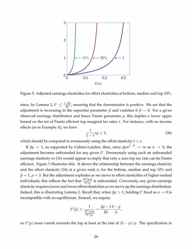
Figure 5: Adjusted earnings elasticities for effort elasticities at bottom, median and top 10%.

since, by Lemma 2, εc ≤ 1−βρβρ , ensuring that the denominator is positive. We see that the

adjustment is increasing in the superstar parameter β and vanishes if β = 0. For a givenobserved earnings distribution and hence Pareto parameter ρ, this implies a lower upperbound on the set of Pareto efficient top marginal tax rates τ. For instance, with no incomeeffects (as in Example A), we have

τ

1− τερ ≤ 1, (36)

which should be compared to erroneously using the effort elasticity ε < ε.

If βρ > 1, as supported by Gabaix-Landier, then, since βρn1ρ−β → ∞ as n → 0, the

adjustment becomes unbounded for any given εc. Erroneously using such an unboundedearnings elasticity in (36) would appear to imply that only a zero top tax rate can be Paretoefficient. Figure 5 illustrates this. It shows the relationship between the earnings elasticityand the effort elasticity (34) at a given rank n, for the bottom, median and top 10% andβ = 1, ρ = 3. But the adjustment explodes as we move to effort elasticities of higher-rankedindividuals; this reflects the fact that W ′(y)y

W(y) is unbounded. Conversely, any given earningselasticity requires lower and lower effort elasticities as we move up the earnings distribution.Indeed, this is illustrating Lemma 2. Recall that, when βρ > 1, holding εc fixed as n → 0 isincompatible with an equilibrium. Instead, we require

εc(y) ≤ 1W ′′(y)yW ′(y)

=βρ− 1

βρ

b− yy

,

so εc(y) must vanish towards the top at least at the rate of (b − y)/y. The specification in

29

Example B features precisely that property and

ε(y) =1

γ + 1b− y

y.

Naively using this effort elasticity in the efficiency test (36), we would erroneously con-clude that the upper bound to the set of Pareto efficient top marginal tax rates is 100%. How-ever, substituting in (34) reveals that the earnings elasticity is in fact constant and equals19

ε =1

γ(βρ− 1)− 1> 0. (37)

The efficiency test for the top marginal tax rate and a given observed earnings distributionbecomes

τ

1− τ

ρ

γ(βρ− 1)− 1≤ 1, (38)

implying a well-defined upper bound on τ strictly less than 1.20

5.4 Macro Elasticities

The earnings elasticities required for Proposition 1 measure partial equilibrium behavioral re-sponses, in the sense that they hold the equilibrium earnings schedule fixed when varyingtaxes. The third scenario is therefore one where the estimated elasticities are macro elastic-ities, which capture the general equilibrium effects of tax changes. This would be the casewhen elasticities are estimated using large tax reforms with aggregate effects or using cross-country comparisons.21 These estimates will capture the fact that the entire equilibriumearnings schedule W(y) shifts in response to the reform, leading to an additional earningsresponse even if an individual were to keep her effort y unchanged.

To fix ideas, consider again a superstar equilibrium for a given tax schedule T, with earn-ings schedule W(y), and pick some earnings level w0 with associated effort y0 = W−1(w0)

and type θ0 = Γ(y0). Suppose we increase marginal tax rates by τ for everyone. We askwhat is the macro elasticity of earnings at w0, incorporating all equilibrium responses, andhow it compares to the correct, partial equilibrium elasticities from Section 4.1.

19γ(βρ− 1) ≥ 1 by Lemma 2.20Using the Gabaix-Landier parameters β = 1 and ρ = 3, this is purely a function of the preference parameter

γ. Depending on γ, any upper bound on the top tax rate in (0, 1) can be justified, and we can always adjustthe underlying skill distribution to make it consistent with the numbers in Gabaix-Landier.

21The former approach includes studies based on time series of aggregate income shares in affected taxbrackets (e.g. Feenberg and Poterba, 1993; Slemrod, 1996; and Saez, 2004) or studies based on panel data (e.g.Feldstein, 1995; Auten and Carroll, 1999; Gruber and Saez, 2002; and Kopczuk, 2005). For the latter approach,see e.g. Prescott (2004) and Davis and Henrekson (2005).

30

Macro Earnings Schedules. We begin with two key observations: First, for any valueof τ, the equilibrium assignment will be the same; i.e., type θ0 will stay matched with thesame firm. The macro elasticity will therefore be akin to the fixed-assignment elasticity fromSection 5.2, where earnings follow the equilibrium output function B(θ0|y). However, thedifference is that the macro elasticity will also incorporate the shift in the earnings schedule,so even when individual θ0 sticks to effort y0, her earnings will not remain at w0. This shiftis due to the shift in profits π(θ0|τ) of the firm that θ0 is matched with in response to thechange in τ.

As a result, the macro earnings response at w0 is determined according to the macroearnings schedule

W0(y|τ) = B(θ0, y)− π(θ0|τ). (39)

To keep the underlying general equilibrium effects tractable, we make two simplifyingassumptions for the purpose of this subsection: (i) We again assume A (and hence B) tobe linear in y; and (ii) we abstract from income effects, so preferences are quasilinear inconsumption. Then individual θ0 chooses her earnings as follows:

w0(τ) ∈ arg maxw

(1− τ)w− T(w)− φ(W−10 (w|τ), θ0) (40)

for some disutility of effort function φ(y, θ) that is increasing and convex in y and super-modular in (y, θ) (to ensure single-crossing). The compensated and uncompensated macroearnings elasticities then coincide and are defined as

ε(w0) =dw0

d(1− τ)

∣∣∣∣τ=0

1− T′(w0)

w0. (41)

Adjusting Macro Elasticities. With these definitions, we have the following result (seeAppendix B.7 for a proof):

Proposition 4. 1. Consider a superstar equilibrium and an individual with earnings w0 andeffort y0 = W−1(w0). Let the macro earnings elasticity ε(w0) be as defined in (41), the fixed-assignment elasticity ε(w0) as in Section 5.2, and the effort elasticity ε(y0) as in (28). Underconditions (i) and (ii), we have

ε(w0) =ε(w0)

Φ(w0)(42)

where

Φ(w0) = 1 +χ(w0)

ε(y0)

1W ′(y0)y0

W(y0)

and χ(w0) =∂W0(y0|τ)∂(1− τ)

∣∣∣∣τ=0

1− T′(w0)

w0. (43)

31

2. If the tax schedule is weakly progressive (T′′(w) ≥ 0 ∀w), then χ(w0) ≤ 0, so the macroelasticity is always smaller than the fixed-assignment elasticity.

As the first part of the Proposition shows, the macro elasticity is closely related to thefixed-assignment elasticity, with an adjustment χ that captures precisely the shift in theequilibrium earnings schedule due to general equilibrium effects. The second part showsthat this adjustment lowers the macro elasticity under a progressive tax schedule. Recall thatProposition 2 showed that the fixed-assignment elasticity is smaller than the correct earn-ings elasticity. A fortiori, any estimate based on the macro elasticity will also underestimatethe correct earnings elasticity when there are superstar effects.

Intuition. When we increase 1 − τ, everyone increases effort in the absence of incomeeffects. Due to complementarities at the firm level, this leads to an increase in profits foreach firm, and hence a reduction in earnings holding effort fixed. The assumption of aprogressive tax schedule guarantees that this downward shift of the earnings schedule leadsto a further increase in effort, and hence profits, because marginal tax rates decrease as wemove down the earnings distribution. The general equilibrium effects therefore eventuallyimply an additional negative effect on earnings, reducing the macro earnings elasticity.

Examples. Proposition 4 can be nicely illustrated using our examples. For the isoelas-tic preferences in Example A with a Pareto skill distribution, Appendix A shows that the

equilibrium earnings schedule is W(y) = ky1

1−βρ + w0 with k = C(1− τ)− βρ

(γ−1)(1−βρ) . Thisimmediately implies that, at the top, the general equilibrium correction in (43) converges to

χ = − βρ

(γ− 1)(1− βρ),

which is negative as predicted by the second part of Proposition 4. We also know that theeffort elasticity is ε = 1/(γ− 1) and the earnings elasticity is ε = 1/(γ(1− βρ)− 1) at thetop by (35). Finally, by (27), the fixed-assignment elasticity at the top is

ε =1

1/ε + βρ=

1(γ− 1)(1− βρ)

< ε.

Taking this together allows us to derive the macro elasticity at the top using (42) and (43):

ε = ε(

1 +χ

ε(1− βρ)

)=

1γ− 1

.

32

The macro elasticity at the top coincides with the effort elasticity. We can therefore summa-rize the relationships between the four elasticity concepts in this case as follows:

ε = ε < ε < ε.

In all three scenarios, the estimated elasticity is smaller than the required superstar earningselasticity ε, with the macro and effort elasticities ε and ε being even smaller than the fixed-assignment elasticity ε.

Similar results can be shown to apply for Example B. Indeed, at the top one finds thatε < ε = 0 < ε < ε.

5.5 Replicating the Superstar Equilibrium without Superstars

We finally address the second question we raised at the beginning of this section: Howwould we have tested for Pareto efficiency if we had believed that the observed earningsdistribution came from a standard economy without superstars, holding fixed the tax Tin place? Clearly, posing this question assumes a positive answer to the following: Arethere economies that replicate the same outcome as in the superstar economy, but withoutsuperstar effects? We shall show this is indeed the case. This amounts to a recalibrationexercise: We pick preferences U(c, w, θ) and a skill distribution F(θ) for a standard Mirrleeseconomy with linear technology where earnings equal effort, w = y, such that, under theearnings tax T, we get the same earnings distribution H(w) as in the superstar economy.We already know that the test formula in Proposition 1 equally applies to this recalibratednon-superstar economy, so the only remaining question is which elasticity corresponds tothe required earnings elasticities for the recalibrated economy.

Recalibrating Preferences. We show first that one can construct U such that the correctelasticities coincide precisely with the fixed-assignment elasticities εu(w), η(w) and εc(w) fromSection (5.2), for example. Fix an earnings tax T and the resulting superstar equilibrium,with effort y(θ), earnings w(θ) = W(y(θ)), output B(θ, y(θ)) and profits

π(θ) ≡ B(θ, y(θ))− w(θ).

Denote by B−1(θ, .) the inverse function of B(θ, .) with respect to its second argument andlet

∆(θ, w) ≡ B−1(θ, w + π(θ)).

33

Using this, define the new utility function

U(c, w, θ) ≡ U(c, ∆(θ, w), θ).

Intuitively, U incorporates the firm level production function B into preferences, holdingagain fixed the equilibrium matching and accounting for the fact that individuals do notearn the entire output because there are profits in the superstar equilibrium. Consider astandard Mirrlees model with linear technology (so output, effort and earnings are all thesame), preferences U, and endowment E + Π with

Π =

ˆπ(θ)dF(θ).

Leave the skill distribution F unchanged. Then we have the following Corollary to Proposi-tion 2 (see Appendix B.8 for a proof):

Corollary 3. In the non-superstar economy with preferences U and earnings tax T, each type θ

chooses the same earnings and consumption as in the superstar economy with preferences U and taxT. The test for Pareto efficiency of T is given by (22) when replacing εc(w) and η(w) by εc(w) andη(w).

In other words, if we believed that the observed earnings distribution was generated bya standard economy with no superstars, we would evaluate the efficiency of the existing taxschedule T based on the same condition as in the superstar economy, but using the lowercompensated earnings elasticity εc(w).

Recalibrating the Skill Distribution. An alternative is to vary the underlying skill distri-bution in the non-superstar economy to match the empirical distribution of earnings in thesuperstar economy, instead of recalibrating preferences. We use Example A to show that thisleads to similar results.

In Example A, both the skill and the equilibrium earnings distribution are (approxi-mately) Pareto, the former with parameter α and the latter with parameter ρ given by (10).Now construct a standard economy with linear production and the same preferences (de-scribed by parameter γ), but with another skill distribution (in fact, a Pareto distributionwith parameter α), such that, under the same tax τ, we replicate the same earnings distri-bution as in the superstar economy. In the standard economy, the Pareto parameter of theearnings distribution will be

ρ =γ− 1

γα,

34

so we need to set α such that ρ = ρ:

α =α

αβ + 1< α.

This is intuitive: To generate the same earnings distribution, the underlying skill inequalityin the non-superstar economy must be higher than in the superstar economy. However,since earnings and effort coincide in the standard economy, the earnings elasticity is simply1/(γ − 1) and hence less than the earnings elasticity in the superstar economy, as we sawin Section 5.3. In other words, accounting for superstars again requires the use of a higherearnings elasticity than in the non-superstars counterfactual, holding fixed the observedearnings distribution.

6 Result 3: Comparative Statics

So far, we have been concerned with how of superstars affect the set of Pareto efficient taxesconditional on a given, observed earnings distribution. In this section, we explore the com-parative static effects of introducing superstar technology holding other fundamentals fixed.These primitives include the parameters of the utility function U and the skill distributionF(θ). In other words, we ask whether, for a given skill distribution and preferences, the in-troduction of superstar effects leads to higher or lower taxes. We also show which statistics,such as elasticities or the parameters of the superstar technology, determine these effects.

6.1 An Efficiency Test in Terms of Primitives

As in Section 3, we begin with a test that any Pareto efficient tax schedule has to satisfy, nowhowever expressed in terms of fundamentals.

Proposition 5. Any Pareto efficient earnings tax T is such that

τ(θ)

1− τ(θ)ξ(θ)

p(θ)−d log

(τ(θ)

1−τ(θ)ξ(θ)

)d log θ

− η(θ)

εc(θ)

y′(θ)θy(θ)

≤ 1 (44)

for all θ, where

p(θ) = −(

1 +d log f (θ)

d log θ

)is the local Pareto parameter of the skill distribution and

ξ(θ) ≡(−∂ log MRS(c(θ), y(θ), θ)

∂ log θ

)−1

≥ 0

35

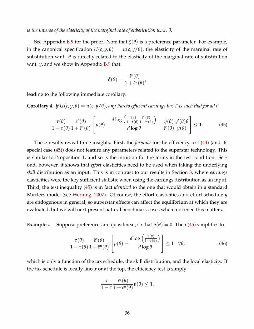
is the inverse of the elasticity of the marginal rate of substitution w.r.t. θ.

See Appendix B.9 for the proof. Note that ξ(θ) is a preference parameter. For example,in the canonical specification U(c, y, θ) = u(c, y/θ), the elasticity of the marginal rate ofsubstitution w.r.t. θ is directly related to the elasticity of the marginal rate of substitutionw.r.t. y, and we show in Appendix B.9 that

ξ(θ) =εc(θ)

1 + εu(θ),

leading to the following immediate corollary:

Corollary 4. If U(c, y, θ) = u(c, y/θ), any Pareto efficient earnings tax T is such that for all θ

τ(θ)

1− τ(θ)

εc(θ)

1 + εu(θ)

p(θ)−d log

(τ(θ)

1−τ(θ)εc(θ)

1+εu(θ)

)d log θ

− η(θ)

εc(θ)

y′(θ)θy(θ)

≤ 1. (45)

These results reveal three insights. First, the formula for the efficiency test (44) (and itsspecial case (45)) does not feature any parameters related to the superstar technology. Thisis similar to Proposition 1, and so is the intuition for the terms in the test condition. Sec-ond, however, it shows that effort elasticities need to be used when taking the underlyingskill distribution as an input. This is in contrast to our results in Section 3, where earningselasticities were the key sufficient statistic when using the earnings distribution as an input.Third, the test inequality (45) is in fact identical to the one that would obtain in a standardMirrlees model (see Werning, 2007). Of course, the effort elasticities and effort schedule yare endogenous in general, so superstar effects can affect the equilibrium at which they areevaluated, but we will next present natural benchmark cases where not even this matters.

Examples. Suppose preferences are quasilinear, so that η(θ) = 0. Then (45) simplifies to

τ(θ)

1− τ(θ)

εc(θ)

1 + εu(θ)

p(θ)−d log

(τ(θ)

1−τ(θ)

)d log θ

≤ 1 ∀θ, (46)

which is only a function of the tax schedule, the skill distribution, and the local elasticity. Ifthe tax schedule is locally linear or at the top, the efficiency test is simply

τ

1− τ

εc(θ)

1 + εu(θ)p(θ) ≤ 1.

36

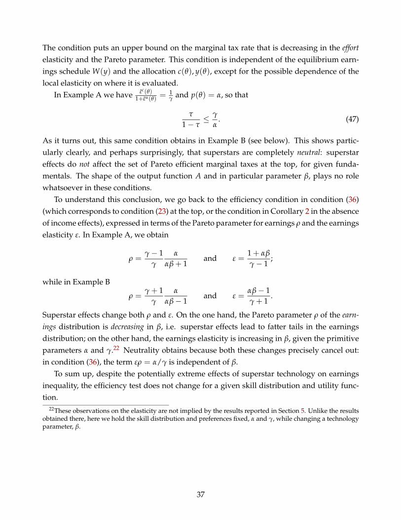
The condition puts an upper bound on the marginal tax rate that is decreasing in the effortelasticity and the Pareto parameter. This condition is independent of the equilibrium earn-ings schedule W(y) and the allocation c(θ), y(θ), except for the possible dependence of thelocal elasticity on where it is evaluated.

In Example A we have εc(θ)1+εu(θ)

= 1γ and p(θ) = α, so that

τ

1− τ≤ γ

α. (47)

As it turns out, this same condition obtains in Example B (see below). This shows partic-ularly clearly, and perhaps surprisingly, that superstars are completely neutral: superstareffects do not affect the set of Pareto efficient marginal taxes at the top, for given funda-mentals. The shape of the output function A and in particular parameter β, plays no rolewhatsoever in these conditions.

To understand this conclusion, we go back to the efficiency condition in condition (36)(which corresponds to condition (23) at the top, or the condition in Corollary 2 in the absenceof income effects), expressed in terms of the Pareto parameter for earnings ρ and the earningselasticity ε. In Example A, we obtain

ρ =γ− 1

γ

α

αβ + 1and ε =

1 + αβ

γ− 1;

while in Example B

ρ =γ + 1

γ

α

αβ− 1and ε =

αβ− 1γ + 1

.

Superstar effects change both ρ and ε. On the one hand, the Pareto parameter ρ of the earn-ings distribution is decreasing in β, i.e. superstar effects lead to fatter tails in the earningsdistribution; on the other hand, the earnings elasticity is increasing in β, given the primitiveparameters α and γ.22 Neutrality obtains because both these changes precisely cancel out:in condition (36), the term ερ = α/γ is independent of β.

To sum up, despite the potentially extreme effects of superstar technology on earningsinequality, the efficiency test does not change for a given skill distribution and utility func-tion.

22These observations on the elasticity are not implied by the results reported in Section 5. Unlike the resultsobtained there, here we hold the skill distribution and preferences fixed, α and γ, while changing a technologyparameter, β.

37

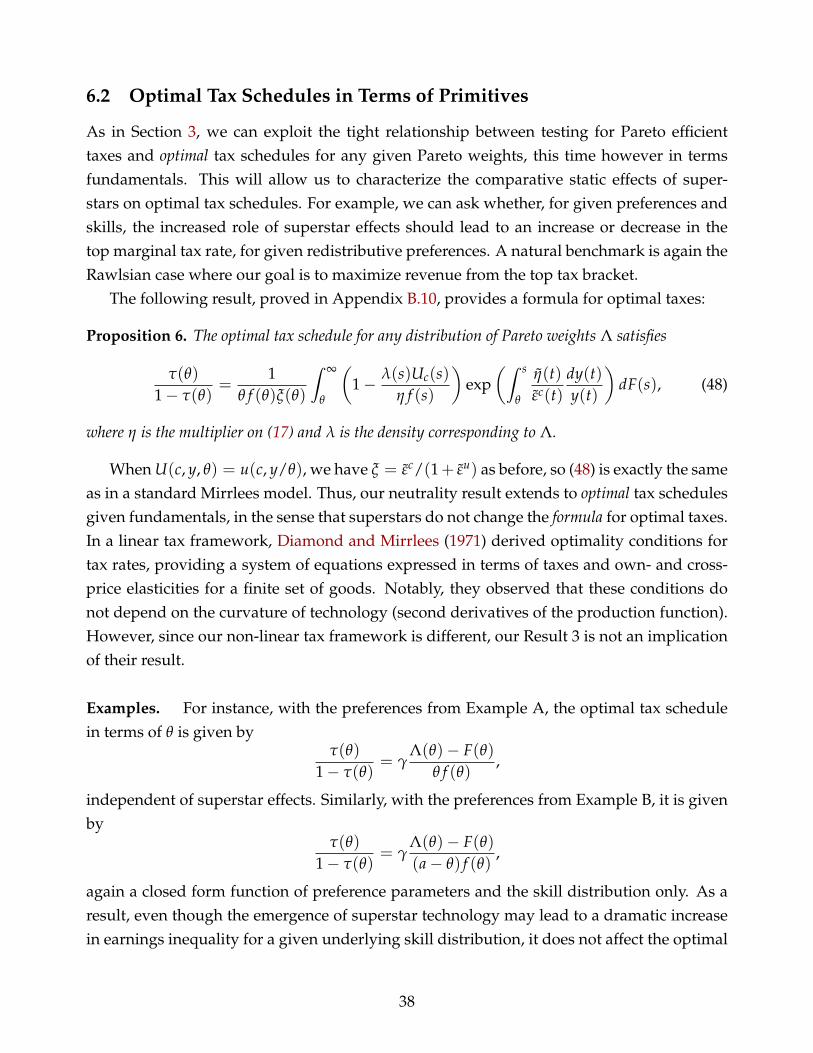
6.2 Optimal Tax Schedules in Terms of Primitives

As in Section 3, we can exploit the tight relationship between testing for Pareto efficienttaxes and optimal tax schedules for any given Pareto weights, this time however in termsfundamentals. This will allow us to characterize the comparative static effects of super-stars on optimal tax schedules. For example, we can ask whether, for given preferences andskills, the increased role of superstar effects should lead to an increase or decrease in thetop marginal tax rate, for given redistributive preferences. A natural benchmark is again theRawlsian case where our goal is to maximize revenue from the top tax bracket.

The following result, proved in Appendix B.10, provides a formula for optimal taxes:

Proposition 6. The optimal tax schedule for any distribution of Pareto weights Λ satisfies

τ(θ)

1− τ(θ)=

1θ f (θ)ξ(θ)

ˆ ∞

θ

(1− λ(s)Uc(s)

η f (s)

)exp

(ˆ s

θ

η(t)εc(t)

dy(t)y(t)

)dF(s), (48)

where η is the multiplier on (17) and λ is the density corresponding to Λ.

When U(c, y, θ) = u(c, y/θ), we have ξ = εc/(1+ εu) as before, so (48) is exactly the sameas in a standard Mirrlees model. Thus, our neutrality result extends to optimal tax schedulesgiven fundamentals, in the sense that superstars do not change the formula for optimal taxes.In a linear tax framework, Diamond and Mirrlees (1971) derived optimality conditions fortax rates, providing a system of equations expressed in terms of taxes and own- and cross-price elasticities for a finite set of goods. Notably, they observed that these conditions donot depend on the curvature of technology (second derivatives of the production function).However, since our non-linear tax framework is different, our Result 3 is not an implicationof their result.

Examples. For instance, with the preferences from Example A, the optimal tax schedulein terms of θ is given by

τ(θ)

1− τ(θ)= γ

Λ(θ)− F(θ)θ f (θ)

,

independent of superstar effects. Similarly, with the preferences from Example B, it is givenby

τ(θ)

1− τ(θ)= γ

Λ(θ)− F(θ)(a− θ) f (θ)

,

again a closed form function of preference parameters and the skill distribution only. As aresult, even though the emergence of superstar technology may lead to a dramatic increasein earnings inequality for a given underlying skill distribution, it does not affect the optimal

38

taxes for any given Pareto weights.23

In the Rawlsian case where positive social welfare weight is put only on the lowest skilltype, we have Λ(θ) = 1 for all θ, so formula (48) simplifies accordingly. With the preferencesand skill distributions assumed in Examples A and B, for instance, the optimal Rawlsianmarginal tax rates are therefore constant and given by

τ

1− τ=

γ

α,

so they are simply the highest Pareto efficient taxes, as given by the upper bound (47).24

Hence, the revenue-maximizing top marginal tax rate is also unaffected by superstar effects.

7 Extensions

In this section, we demonstrate that our results are not specific to the simple one-to-onematching model considered so far. They extend to alternative and more general settingswith superstar effects, including the first- and second-generation span-of-control models weturn to next.

7.1 Span-of-Control with Identical Workers

Managers and Workers. We begin with the canonical span-of-control model going backto Lucas (1978) and Rosen (1982), adding an intensive effort margin for managers. There isa unit mass of managers with skill θ ∼ F who provide effective effort y as before. Ratherthan being matched with an exogenous set of firms, managers own the firms and hire ahomogeneous labor input to produce output. There is a unit mass of identical workers whoeach supply one unit of labor inelastically at zero cost. A manager who exerts y units ofeffective effort and who hires L units of labor produces output according to

A(L, y),

23These results imply that a given individual of type θ faces the same optimal marginal tax rate, no matterwhether technology features superstar effects or not. This is the standard way of reporting the predictions ofoptimal nonlinear taxes in the literature. Since the distribution of θ is fixed and since earnings are monotone inθ, it is equivalent to reporting marginal taxes as a function of the quantiles of the earnings distribution, a usefulnormalization (i.e. it answers “what is the tax on the top x%?”). In general, this does not mean that the taxschedule when written in terms of earnings, T(w), is unchanged. The reason, of course, is that the distributionof earnings changes when superstar effects emerge.

24More generally, formula (48) for the Rawlsian case is the integral version of (44) when it holds as an equalityeverywhere.

39

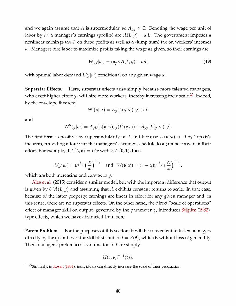
and we again assume that A is supermodular, so ALy > 0. Denoting the wage per unit oflabor by ω, a manager’s earnings (profits) are A(L, y) − ωL. The government imposes anonlinear earnings tax T on these profits as well as a (lump-sum) tax on workers’ incomesω. Managers hire labor to maximize profits taking the wage as given, so their earnings are

W(y|ω) = maxL

A(L, y)−ωL (49)

with optimal labor demand L(y|ω) conditional on any given wage ω.

Superstar Effects. Here, superstar effects arise simply because more talented managers,who exert higher effort y, will hire more workers, thereby increasing their scale.25 Indeed,by the envelope theorem,

W ′(y|ω) = Ay(L(y|ω), y) > 0

andW ′′(y|ω) = AyL(L(y|ω), y)L′(y|ω) + Ayy(L(y|ω), y).

The first term is positive by supermodularity of A and because L′(y|ω) > 0 by Topkis’stheorem, providing a force for the managers’ earnings schedule to again be convex in theireffort. For example, if A(L, y) = Lαy with α ∈ (0, 1), then

L(y|ω) = y1

1−α

( α

ω

) 11−α and W(y|ω) = (1− α)y

11−α

( α

ω

) α1−α ,

which are both increasing and convex in y.Ales et al. (2015) consider a similar model, but with the important difference that output

is given by θγ A(L, y) and assuming that A exhibits constant returns to scale. In that case,because of the latter property, earnings are linear in effort for any given manager and, inthis sense, there are no superstar effects. On the other hand, the direct “scale of operations”effect of manager skill on output, governed by the parameter γ, introduces Stiglitz (1982)-type effects, which we have abstracted from here.

Pareto Problem. For the purposes of this section, it will be convenient to index managersdirectly by the quantiles of the skill distribution t = F(θ), which is without loss of generality.Then managers’ preferences as a function of t are simply

U(c, y, F−1(t)).

25Similarly, in Rosen (1981), individuals can directly increase the scale of their production.

40

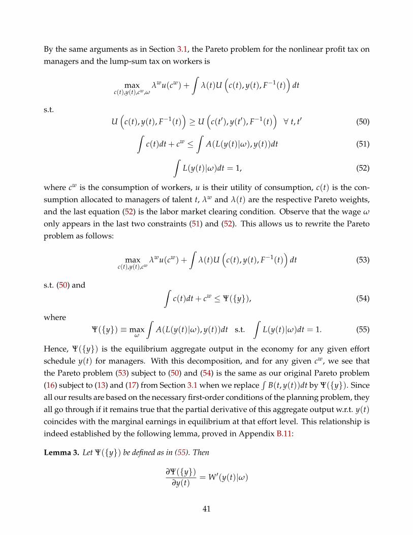
By the same arguments as in Section 3.1, the Pareto problem for the nonlinear profit tax onmanagers and the lump-sum tax on workers is

maxc(t),y(t),cw,ω

λwu(cw) +

ˆλ(t)U

(c(t), y(t), F−1(t)

)dt

s.t.U(

c(t), y(t), F−1(t))≥ U

(c(t′), y(t′), F−1(t)

)∀ t, t′ (50)

ˆc(t)dt + cw ≤

ˆA(L(y(t)|ω), y(t))dt (51)

ˆL(y(t)|ω)dt = 1, (52)

where cw is the consumption of workers, u is their utility of consumption, c(t) is the con-sumption allocated to managers of talent t, λw and λ(t) are the respective Pareto weights,and the last equation (52) is the labor market clearing condition. Observe that the wage ω

only appears in the last two constraints (51) and (52). This allows us to rewrite the Paretoproblem as follows:

maxc(t),y(t),cw

λwu(cw) +

ˆλ(t)U

(c(t), y(t), F−1(t)

)dt (53)

s.t. (50) and ˆc(t)dt + cw ≤ Ψ({y}), (54)

whereΨ({y}) ≡ max

ω

ˆA(L(y(t)|ω), y(t))dt s.t.

ˆL(y(t)|ω)dt = 1. (55)

Hence, Ψ({y}) is the equilibrium aggregate output in the economy for any given effortschedule y(t) for managers. With this decomposition, and for any given cw, we see thatthe Pareto problem (53) subject to (50) and (54) is the same as our original Pareto problem(16) subject to (13) and (17) from Section 3.1 when we replace

´B(t, y(t))dt by Ψ({y}). Since

all our results are based on the necessary first-order conditions of the planning problem, theyall go through if it remains true that the partial derivative of this aggregate output w.r.t. y(t)coincides with the marginal earnings in equilibrium at that effort level. This relationship isindeed established by the following lemma, proved in Appendix B.11:

Lemma 3. Let Ψ({y}) be defined as in (55). Then

∂Ψ({y})∂y(t)

= W ′(y(t)|ω)

41

for any ω and t.

Because of Lemma 3, all of our results in Propositions 1 to 6 immediately extend to theearnings tax for managers in this model.

7.2 Span-of-Control with Heterogeneous Workers

In this section, we demonstrate how our results extend to modern, richer models of orga-nizational hierarchies, including those developed by Garicano and Rossi-Hansberg (2004,2006) and, most recently, Fuchs et al. (2015).26 Here, higher-skilled managers not only lever-age their talent by hiring more workers, they are also matched with teams of higher-skilledworkers, generating yet an additional source of superstar effects. Moreover, these modelsallow for an endogenous sorting of individuals into hierarchical layers.

Knowledge-based Hierarchies. As in Garicano and Rossi-Hansberg (2004) and Fuchset al. (2015), we consider the simplest possible setting in which hierarchies consist of twolayers, managers and workers (or producers).27 In fact, we closely follow the setup in Fuchset al. (2015) where individuals use time and knowledge to solve problems, with the onlyaddition that we incorporate an intensive effort margin to generate a role for taxes.

There is free entry of risk-neutral firms. Each firm hires one manager and n workers,where n may be non-integer. There is also a continuum of heterogeneous individuals ofunit mass indexed by their talent t who are each endowed with one unit of time and canbecome either managers or workers. As in the preceding subsection, we associate t withthe quantiles of the skill distribution F, so t ∼ U(0, 1). Individuals provide effective efforty and have preferences U(c, y, F−1(t)). For the purposes of this subsection, w.l.o.g. we alsonormalize effective effort such that y ∈ [0, 1].

Workers and Managers. Each worker is faced with a problem of random difficulty x ∼U(0, 1), distributed independently across problems. She manages to solve the problem onher own if her effective effort exceeds the problem’s difficulty level. Formally, if her effectiveeffort is yp, she can solve the problem whenever x < yp, thus with probability yp. If she fails,she can seek help from a manager. It costs a manager h units of her time to help a workerwith an unsolved problem. Hence, if a manager is matched with workers who provide effort

26See also Garicano and Rossi-Hansberg (2015) for a recent survey of this literature.27Extending our results to larger numbers of layers, such as in Garicano and Rossi-Hansberg (2006), is

straightforward.

42

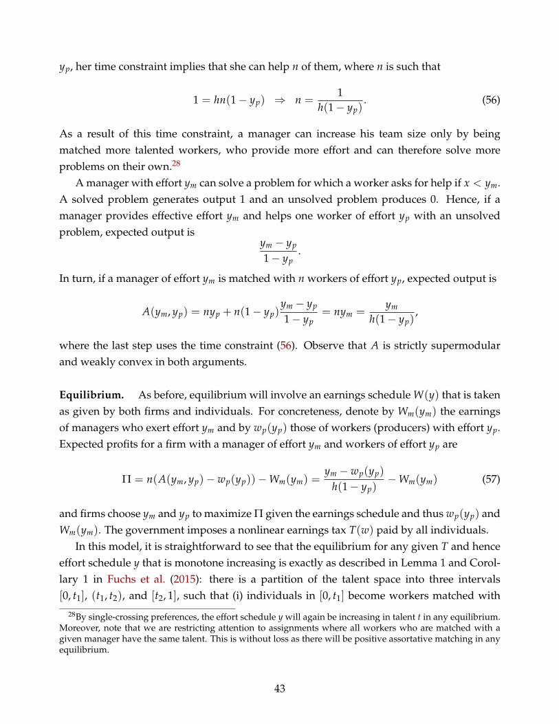
yp, her time constraint implies that she can help n of them, where n is such that

1 = hn(1− yp) ⇒ n =1

h(1− yp). (56)

As a result of this time constraint, a manager can increase his team size only by beingmatched more talented workers, who provide more effort and can therefore solve moreproblems on their own.28

A manager with effort ym can solve a problem for which a worker asks for help if x < ym.A solved problem generates output 1 and an unsolved problem produces 0. Hence, if amanager provides effective effort ym and helps one worker of effort yp with an unsolvedproblem, expected output is

ym − yp

1− yp.

In turn, if a manager of effort ym is matched with n workers of effort yp, expected output is

A(ym, yp) = nyp + n(1− yp)ym − yp

1− yp= nym =

ym

h(1− yp),

where the last step uses the time constraint (56). Observe that A is strictly supermodularand weakly convex in both arguments.

Equilibrium. As before, equilibrium will involve an earnings schedule W(y) that is takenas given by both firms and individuals. For concreteness, denote by Wm(ym) the earningsof managers who exert effort ym and by wp(yp) those of workers (producers) with effort yp.Expected profits for a firm with a manager of effort ym and workers of effort yp are

Π = n(A(ym, yp)− wp(yp))−Wm(ym) =ym − wp(yp)

h(1− yp)−Wm(ym) (57)

and firms choose ym and yp to maximize Π given the earnings schedule and thus wp(yp) andWm(ym). The government imposes a nonlinear earnings tax T(w) paid by all individuals.

In this model, it is straightforward to see that the equilibrium for any given T and henceeffort schedule y that is monotone increasing is exactly as described in Lemma 1 and Corol-lary 1 in Fuchs et al. (2015): there is a partition of the talent space into three intervals[0, t1], (t1, t2), and [t2, 1], such that (i) individuals in [0, t1] become workers matched with

28By single-crossing preferences, the effort schedule y will again be increasing in talent t in any equilibrium.Moreover, note that we are restricting attention to assignments where all workers who are matched with agiven manager have the same talent. This is without loss as there will be positive assortative matching in anyequilibrium.

43

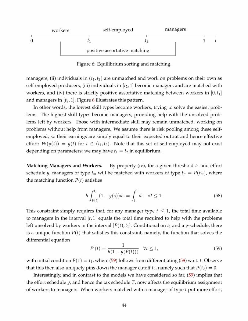
0 t1 t2 1 t

workers self-employed managers

positive assortative matching

Figure 6: Equilibrium sorting and matching.

managers, (ii) individuals in (t1, t2) are unmatched and work on problems on their own asself-employed producers, (iii) individuals in [t2, 1] become managers and are matched withworkers, and (iv) there is strictly positive assortative matching between workers in [0, t1]

and managers in [t2, 1]. Figure 6 illustrates this pattern.In other words, the lowest skill types become workers, trying to solve the easiest prob-

lems. The highest skill types become managers, providing help with the unsolved prob-lems left by workers. Those with intermediate skill may remain unmatched, working onproblems without help from managers. We assume there is risk pooling among these self-employed, so their earnings are simply equal to their expected output and hence effectiveeffort: W(y(t)) = y(t) for t ∈ (t1, t2). Note that this set of self-employed may not existdepending on parameters: we may have t1 = t2 in equilibrium.

Matching Managers and Workers. By property (iv), for a given threshold t1 and effortschedule y, managers of type tm will be matched with workers of type tp = P(tm), wherethe matching function P(t) satisfies

hˆ t1

P(t)(1− y(s))ds =

ˆ 1

tds ∀t ≤ 1. (58)

This constraint simply requires that, for any manager type t ≤ 1, the total time availableto managers in the interval [t, 1] equals the total time required to help with the problemsleft unsolved by workers in the interval [P(t), t1]. Conditional on t1 and a y-schedule, thereis a unique function P(t) that satisfies this constraint, namely, the function that solves thedifferential equation

P′(t) =1

h(1− y(P(t)))∀t ≤ 1, (59)

with initial condition P(1) = t1, where (59) follows from differentiating (58) w.r.t. t. Observethat this then also uniquely pins down the manager cutoff t2, namely such that P(t2) = 0.

Interestingly, and in contrast to the models we have considered so far, (59) implies thatthe effort schedule y, and hence the tax schedule T, now affects the equilibrium assignmentof workers to managers. When workers matched with a manager of type t put more effort,

44

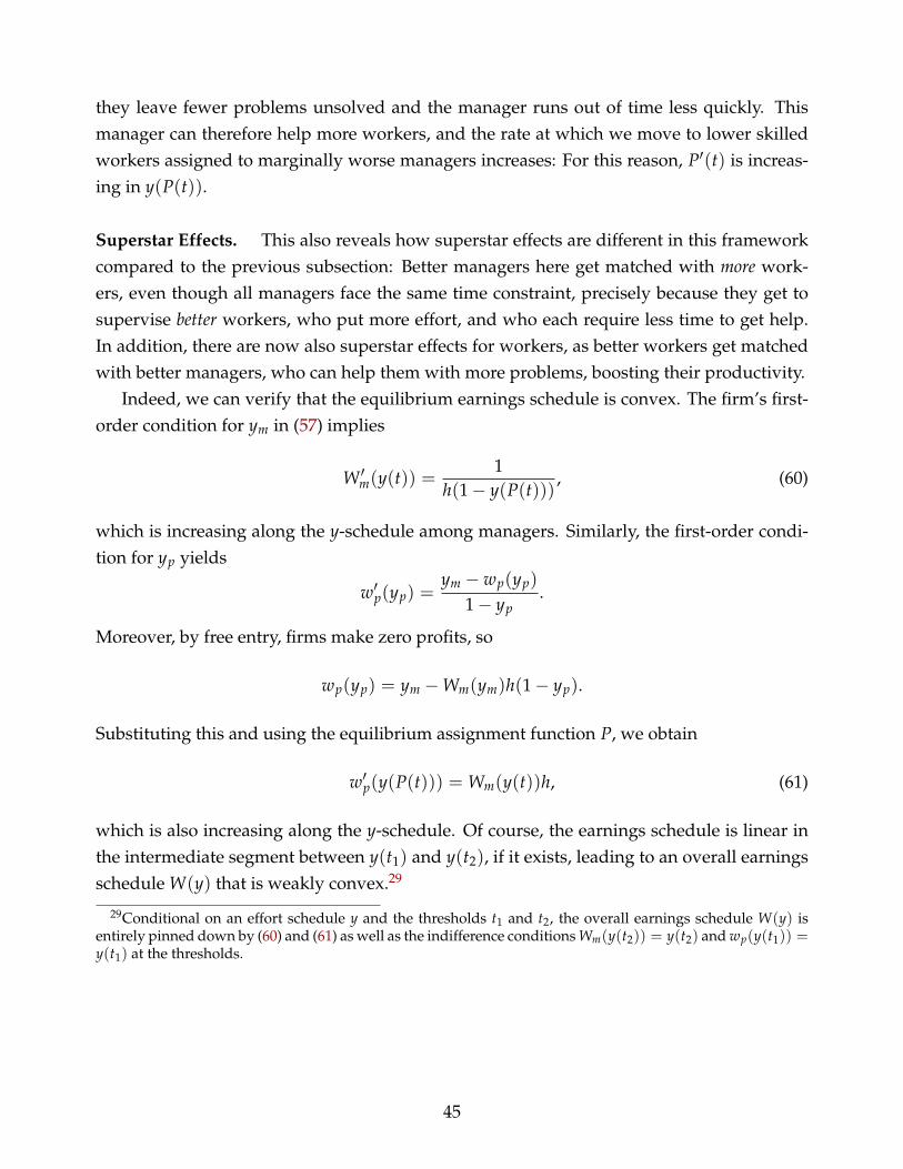
they leave fewer problems unsolved and the manager runs out of time less quickly. Thismanager can therefore help more workers, and the rate at which we move to lower skilledworkers assigned to marginally worse managers increases: For this reason, P′(t) is increas-ing in y(P(t)).

Superstar Effects. This also reveals how superstar effects are different in this frameworkcompared to the previous subsection: Better managers here get matched with more work-ers, even though all managers face the same time constraint, precisely because they get tosupervise better workers, who put more effort, and who each require less time to get help.In addition, there are now also superstar effects for workers, as better workers get matchedwith better managers, who can help them with more problems, boosting their productivity.

Indeed, we can verify that the equilibrium earnings schedule is convex. The firm’s first-order condition for ym in (57) implies

W ′m(y(t)) =1

h(1− y(P(t))), (60)

which is increasing along the y-schedule among managers. Similarly, the first-order condi-tion for yp yields

w′p(yp) =ym − wp(yp)

1− yp.

Moreover, by free entry, firms make zero profits, so

wp(yp) = ym −Wm(ym)h(1− yp).

Substituting this and using the equilibrium assignment function P, we obtain

w′p(y(P(t))) = Wm(y(t))h, (61)

which is also increasing along the y-schedule. Of course, the earnings schedule is linear inthe intermediate segment between y(t1) and y(t2), if it exists, leading to an overall earningsschedule W(y) that is weakly convex.29

29Conditional on an effort schedule y and the thresholds t1 and t2, the overall earnings schedule W(y) isentirely pinned down by (60) and (61) as well as the indifference conditions Wm(y(t2)) = y(t2) and wp(y(t1)) =y(t1) at the thresholds.

45

Pareto Problem. By the same arguments as in Section 3.1, we are now ready to write downthe Pareto problem for the earnings tax T:

maxc,y,P,t1,t2

ˆ 1

0λ(t)U(c(t), y(t), F−1(t))dt

s.t. ˆ 1

0c(t)dt ≤

ˆ 1

t2

y(t)h(1− y(P(t)))

dt +ˆ t2

t1

y(t)dt, (62)

(50), (59) and P(1) = t1, P(t2) = 0. The first integral on the right-hand side of (62) is totaloutput produced by matched agents (integrating over managers), and the second is totaloutput produced by the self-employed.

A key observation is again that P, t1 and t2 only enter constraints (59) and (62), whichallows us to decompose the Pareto problem as follows:

maxc,y

ˆ 1

0λ(t)U(c(t), y(t), F−1(t))dt (63)

s.t. (50) and ˆ 1

0c(t)dt ≤ Ψ({y}), (64)

where

Ψ({y}) = maxP,t1,t2

ˆ 1

t2

y(t)h(1− y(P(t)))

dt +ˆ t2

t1

y(t)dt (65)

s.t. (59) and P(1) = t1, P(t2) = 0. Hence, similar to the previous subsection, Ψ({y}) is ag-gregate output in the economy under the equilibrium assignment for any given (monotone)effort schedule y.30 The Pareto problem (63) s.t. (50) and (64) is therefore again identical toour original Pareto problem (16) subject to (13) and (17) from Section 3.1 when we replace´

B(t, y(t))dt by Ψ({y}). Since all our results are based on the necessary first-order condi-tions of the planning problem, they all go through if it remains true that the partial derivativeof this aggregate output w.r.t. y(t) coincides with the marginal earnings in equilibrium atthat effort level. The following lemma again establishes precisely this relationship:

Lemma 4. Let Ψ({y}) be defined as in (65). Then

∂Ψ({y})∂y(t)

= W ′(y(t))

for all t.

30By single-crossing and (50), any incentive compatible effort schedule y must be monotone, so we willevaluate Ψ only for monotone schedules.

46

The proof is in Appendix B.12. Despite the additional complexities of this model, inparticular the richer effects of taxes on equilibrium matching, this implies again that ourresults extend to the earnings tax for both workers and managers in this model.

7.3 A General Production Function Approach

Both of our previous extensions concluded by showing that, in equilibrium, there existsan aggregate production function Ψ({y}) that maximizes total output, given effort choices{y}, as well as the property that marginal earnings W ′(y(t)) equal the derivative of Ψ withrespect to y(t). This suggests starting at the end of this line of reasoning, in a more generaland abstract manner.

To pursue this, we now simply postulate that there exists an aggregate production func-tion

Φ(M),

where M denotes a positive measure over the set of possible effort levels Y. Typically, Φ(M)

will be defined by maximizing output over all feasible allocations, given the distribution ofeffort M. We also assume that the equilibrium measure M maximizes aggregate profits

Φ(M)−ˆ

W(y)dM.

This may be taken as a defining property of competitive equilibria.Starting with a distribution of types t ∈ [0, 1], an allocation y : [0, 1] → Y induces a

particular measure My. DefineΨ({y}) ≡ Φ(My).

It then follows that in equilibrium {y}maximizes

Ψ({y})−ˆ

W(y(t))dt.

A necessary condition is that

W ′(y(t)) =∂Ψ({y})

∂y(t), (66)

the desired marginal condition.31 Our results then follow directly for this more generalformulation.

31More formally, by ∂∂y Ψ({y}) we mean the following. The Fréchet derivative of Ψ at some {y} in direction

h is a linear function∂Ψ({y}, h) =

ˆδ(t)dh(t).

47

It is worth pointing out that this formulation allows for arbitrary effects of taxes on theequilibrium assignment. This is because taxes can distort the effort schedule y(t), which inturn affects matching. However, the marginal condition (66) implies a form of efficiency con-ditional on a given effort schedule, as (private) marginal earnings coincide with the (social)marginal product. In other words, taxes distort the assignment through their effect on ef-fort, but not conditional on effort. Distortions conditional on effort could arise, for instance,when part of the matching surplus is untaxed, as in Jaffe and Kominers (2014). These issuesare not inherently related to superstar effects. They would emerge, more broadly, in any Roymodel with untaxed activities, such as household production or an informal sector.

8 Conclusion

This paper extends the Mirrlees optimal taxation model by enriching the labor market toincorporate an assignment problem between workers and firms. As first shown by Rosen(1981), assignment models of this sort are capable of producing superstar phenomena, whereinnate skill differences are greatly magnified in terms of earnings. Despite the potential todramatically increase inequality, our results show that these superstar effects do not providea basis for higher taxation. Indeed, depending on the interpretation, they are either neutralor provide a force for lower taxes.

It is worth clarifying that this force for lower taxes does not, by itself, imply that taxesat the top of the earnings distribution should be low or lower than current tax rates. Otherforces or considerations, unrelated to superstars, may be at play at the top shaping the opti-mal level of taxes. Here we mention a few.

Stiglitz effects. As mentioned in the introduction, an active current literature explores howgeneral equilibrium effects affect the optimal policy when tax instruments are limited. Thisliterature revisits Stiglitz (1982) but using richer Roy models where relative wages acrossdifferent sectors enter incentive constraints and tax policy seeks to manipulate wages to relaxthese constraints, typically implying lower taxes at the top. Since these “Stiglitz effects” areseparate from superstar effects, we have abstracted from them in this paper.

Inefficiencies and uncertainty. It has been argued that some top earners earn excessive in-comes not just because of superstar effects, but because their pay exceeds their marginalproduct. This could be due to rent-seeking (Rothschild and Scheuer, 2014a), inefficient bar-gaining (Piketty et al., 2014) or other inefficiencies (Rothschild and Scheuer, 2014b; Lock-

for some δ : [0, 1]→ R. We define∂

∂y(t)Ψ({y}) = δ(t).

48

wood et al., 2014) at the top of the income distribution. On the other hand, pay can be belowmarginal product, for instance for innovators that only appropriate a fraction of the value oftheir innovations, as in endogenous growth models. Finally, some top incomes may be dueto luck. Inefficiencies and uncertainty of this kind provide Pigouvian and insurance motivesfor taxes. However, these issues arise even in standard Mirrlees models without superstareffects. To isolate the role of superstars, we have, therefore, ignored them here.

Low effort elasticities. One may argue that superstars at the top of the earnings distributionhave very low labor supply elasticities at the margin, because their pay and effort are sohigh or because they are intrinsically motivated. Of course, this argument for higher taxesat the top is completely unrelated to the presence of superstar effects and is also presentin a standard Mirrleesian model. Whatever the effort elasticity of top earners, our secondresult shows that this elasticity needs to be adjusted upwards when accounting for superstareffects. For instance, our Example B features an effort elasticity that converges to zero at thetop, yet the correct earnings elasticity is a positive constant.

References

Ales, Laurence and Christopher Sleet, “Taxing Top Incomes,” Working Paper, 2015. 1

, Andres Bellofatto, and Jessie Wang, “Taxing Atlas: Using Firm Data to Derive OptimalIncome Tax Rates,” Working Paper, 2015. 1, 7.1

Ales, Laurence, Musab Kurnaz, and Christopher Sleet, “Tasks, Talents, and Taxes,” Ameri-can Economic Review, 2014, forthcoming. 1

Auten, Gerald and Robert Carroll, “The Effect of Income Taxes on Household Income,”Review of Economics and Statistics, 1999, 81, 681–693. 21

Blundell, Richard, Alan Duncan, and Costas Meghir, “Estimating Labor Supply ResponsesUsing Tax Reforms,” Econometrica, 1998, 66, 827–862. 18

Chetty, Raj, “Bounds on Elasticities with Optimization Frictions: A Synthesis of Micro andMacro Evidence on Labor Supply,” Econometrica, 2012, 80 (969-1018). 15

Davis, Steven and Magnus Henrekson, “Tax Effects on Work Activity, Industry Mix andShadow Economy Size: Evidence From Rich-Country Comparisons,” in Salvador et al.,ed., Labour Supply and Incentives to Work in Europe, Edward Elgar Press, 2005. 21

Diamond, Peter and James Mirrlees, “Optimal Taxation and Public Production: I–Production Efficiency,” American Economic Review, March 1971, 61 (1), 8–27. 2.1, 6.2

49

Edmans, Alex and Xavier Gabaix, “Executive Compensation: A Modern Primer,” WorkingPaper, 2015. 1

Eissa, Nada and Hilary Hoynes, “The Earned Income Tax Credit and the Labor Supply ofMarried Couples,” NBER Working Paper 6856, 1998. 18

Feenberg, Daniel and James Poterba, “Income Inequality and the Incomes of Very High-Income Taxpayers: Evidence from Tax Returns,” in James Poterba, ed., Tax Policy and theEconomy, Vol. 7, MIT Press, 1993, pp. 145–177. 21

Feldstein, Martin, “The Effect of Marginal Tax Rates on Taxable Income: A Panel Study ofthe 1986 Tax Reform Act,” Journal of Political Economy, 1995, 103, 551–572. 21

Fuchs, William, Luis Garicano, and Luis Rayo, “Optimal Contracting and the Organizationof Knowledge,” Review of Economic Studies, 2015, forthcoming. 7.2, 7.2, 7.2

Gabaix, Xavier and Augustin Landier, “Why Has CEO Pay Increased So Much?,” QuarterlyJournal of Economics, 2008, 123, 49–100. 1, 1, 2.1, 2.3, 17

Garicano, Luis, “Hierarchies and the Organization of Knowledge in Production,” Journal ofPolitical Economy, October 2000, 108 (5), 874–904. 1

and Esteban Rossi-Hansberg, “Inequality and the Organization of Knowledge,” Ameri-can Economic Review, 2004, 94, 197–202. 7.2, 7.2

and , “Organization and Inequality in a Knowledge Economy,” Quarterly Journal ofEconomics, 2006, 121, 1383–1435. 7.2, 27

and , “Knowledge-Based Hierarchies: Using Organizations to Understand the Econ-omy,” Annual Review of Economics, 2015, 7, 1–30. 1, 26

Gruber, Jon and Emmanuel Saez, “The Elasticity Of Taxable Income: Evidence And Impli-cations,” Journal of Public Economics, 2002, 84, 1–32. 21

Hausman, Jerry, “Taxes and Labor Supply,” in Alan Auerbach and Martin Feldstein, eds.,Handbook of Public Economics, Vol. 1, Elsevier, 1985, chapter 4, pp. 213–263. 5.3

Jaffe, Sonia and Scott Kominers, “Taxation in Matching Markets,” Working Paper, 2014. 7.3

Keane, Michael, “Labor Supply and Taxes: A Survey,” Journal of Economic Literature, 2011,49, 961–1075. 15

and Richard Rogerson, “Micro and Macro Labor Supply Elasticities: A Reassessment ofConventional Wisdom,” Journal of Economic Literature, 2012, 50, 464–76. 15

50

Kopczuk, Wojciech, “Tax Bases, Tax Rates and the Elasticity of Reported Income,” Journal ofPublic Economics, 2005, 89, 2093–2119. 21

Lockwood, Ben, Charles Nathanson, and Glen Weyl, “Taxation and the Allocation of Tal-ent,” Working Paper, 2014. 8

Lucas, Robert, “On the Size Distribution of Business Firms,” Bell Journal of Economics, 1978,9, 508–523. 1, 7.1

MaCurdy, Thomas, “An Empirical Model of Labor Supply in a Life-Cycle Setting,” Journalof Political Economy, 1981, 89, 1059–1085. 18

Mirrlees, James, “An Exploration in the Theory of Optimum Income Taxation,” Review ofEconomic Studies, 1971, 38 (2), 175–208. 1, 2.1

Piketty, Thomas, Emmanuel Saez, and Stefanie Stantcheva, “Optimal Taxation of Top La-bor Incomes: A Tale of Three Elasticities,” American Economic Journal: Economic Policy,2014, 6, 230–271. 1, 8

Prescott, Edward, “Why Do Americans Work so Much More Than Europeans?,” FederalReserve Bank of Minneapolis Quarterly Review, 2004, 28, 2–13. 21

Rosen, Sherwin, “The Economics of Superstars,” American Economic Review, 1981, 71, 845–858. 1, 2, 3, 25, 8

, “Authority, Control, and the Distribution of Earnings,” Bell Journal of Economics, 1982, 13,311–323. 1, 7.1

Rothschild, Casey and Florian Scheuer, “Redistributive Taxation in the Roy Model,” Quar-terly Journal of Economics, 2013, 128, 623–668. 1

and , “Optimal Taxation with Rent-Seeking,” Working Paper, 2014. 1, 8

and , “A Theory of Income Taxation under Multidimensional Skill Heterogeneity,”Working Paper, 2014. 8

Saez, Emmanuel, “Using Elasticities to Derive Optimal Income Tax Rates,” Review of Eco-nomic Studies, 2001, 68 (1), 205–29. 1, 1, 4.2, 5.3

, “Reported Incomes and Marginal Tax Rates, 1960-2000,” in James Poterba, ed., Tax Policyand the Economy, Vol. 18, MIT Press, 2004, pp. 117–174. 21

, “Do Taxpayers Bunch at Kink Points?,” American Economic Journal: Economic Policy, 2010,2, 180–212. 18

51

, Joel Slemrod, and Seth Giertz, “The Elasticity of Taxable Income with Respect toMarginal Tax Rates: A Critical Review,” Journal of Economic Perspectives, 2012, 50, 3–50.15

Samuelson, Paul, The Foundations of Economic Analysis, Cambridge, MA: Harvard UniversityPress, 1947. 5.2

Sattinger, Michael, “Assignment Models of the Distribution of Earnings,” Journal of Eco-nomic Literature, 1993, 91, 831–880. 1

Scheuer, Florian, “Entrepreneurial Taxation with Endogenous Entry,” American EconomicJournal: Economic Policy, 2014, 6, 126–163. 1

Slemrod, Joel, “High-Income Families and the Tax Changes of the 1980s: The Anatomy ofBehavioral Response,” in Martin Feldstein and James Poterba, eds., The Empirical Founda-tions of Household Taxation, University of Chicago Press, 1996, pp. 169–189. 21

Stiglitz, Joseph, “Self-Selection and Pareto Efficient Taxation,” Journal of Public Economics,1982, 17, 213–240. 1, 7.1, 8

Terviö, Marko, “The difference that CEOs make: An assignment model approach,” TheAmerican Economic Review, 2008, pp. 642–668. 1, 2, 2.1

Werning, Iván, “Pareto Efficient Income Taxation,” Mimeo, MIT, 2007. 1, 4, 4.2, 4.2, 6.1

Ziliak, James and Thomas Kniesner, “Estimating Life Cycle Labor Supply Tax Effects,”Journal of Political Economy, 1999, 107, 326–359. 18

A Appendix: Derivations for Examples A and B

A.1 Example A

Exact Earnings Schedule and Approximate Pareto Skill Distribution. We begin with Example Ain Section 2.3 and construct the skill distribution F(θ) as claimed in the text. Taking W(y) as given by(9), individuals solve

maxy

(1− τ)W(y)− 1γ

(yθ

)γ.

The first-order condition is

(1− τ)κ

1− βρ

(κβρ

1− βρ+ y) 1

1−βρ−1

= yγ−1θ−γ

52

and the second-order condition for a maximum is satisfied if γ(1− βρ) > 1. Substituting y(n) from(8) for y yields

θ(1− τ)1γ

(κ

1− βρ

) 1γ(

κ

1− βρnβ− 1

ρ

) βρ1−βρ

1γ

=

(κ

1− βρnβ− 1

ρ − κβρ

1− βρ

) γ−1γ

,

which simplifies after substituting κ to

θ(1− τ)1γ n−

βγ =

(κ

1− βρ

) γ−1γ (

nβ− 1ρ − βρ

) γ−1γ

or equivalently

θ = (1− τ)−1γ

(κ

1− βρ

) γ−1γ(

nβ

γ−1

(n−

1−βρρ − βρ

)) γ−1γ

.

This implicitly defines n = 1− F(θ) given θ and hence F(θ). Rewriting this as

θ = (1− τ)−1γ

(κ

1− βρ

) γ−1γ(

n−γ(1−βρ)−1(γ−1)ρ − βρn

βγ−1

) γ−1γ

reveals that, if γ(1− βρ) > 1, then for sufficiently small for n ≈ 0 (i.e., at the top of the skill distribu-tion)

θ ≈ (1− τ)−1γ

(κ

1− βρ

) γ−1γ

n−γ(1−βρ)−1

γρ .

Hence,n = 1− F(θ) ≈ (θ/θ)α

for some θ, withα =

γρ

γ(1− βρ)− 1.

In other words, θ has a Pareto tail with parameter α > 0. Conversely, solving for ρ yields (10) and,since α > 0, we indeed must have γ(1− βρ) > 1.

Exact Pareto Skill Distribution and Approximate Earnings Schedule. We next derive the equi-librium earnings schedule for Example A when F(θ) = 1− (θ/θ)α, that is, F is a Pareto distributionfor all θ ≥ θ. We do so by guessing and verifying a schedule of the form W(y) = kyδ + w0 for someparameters k, δ, w0. Taking τ and W(y) as given, individuals solve

maxy

(1− τ)kyδ − 1γ

(yθ

)γ.

The first-order condition yields the y-schedule

y(θ) = θγ

γ−δ (δk(1− τ))1

γ−δ (67)

as well as its inverseΓ(y) = y

γ−δγ (δk(1− τ))−

1γ .

53

Note that we require δ < γ, which we will verify below. We know from the assignment condition (5)that W ′(y) = By(Γ(y), y), so using B(θ, y) = θ−αβθαβy, this becomes

δky = yαβ γ−δγ (δk(1− τ))−

αβγ θ−αβ.

Matching coefficients requires

δk = (δk(1− τ))−αβγ θ−αβ

andδ− 1 = αβ

γ− δ

γ.

Solving this yields

δ = γαβ + 1αβ + γ

as claimed in the text andk =

1γ

αβ + γ

αβ + 1(1− τ)−

αβγ+αβ θ

− αβγγ+αβ .

Observe that we indeed have δ < γ because γ > 1 by assumption. Using these expressions for δ andk in (67) yields the equilibrium effort schedule y(θ). Finally, w0 is determined such that profits of thelowest firm x = 0 are zero, so B(θ, y(θ)) = y(θ) = W(y(θ)) = ky(θ)δ + w0.

Using n = 1− F and (67), we can write

y(n) = Cn−αβ+γ

α(γ−1) = Cnβ− 1ρ

for some constant C, where the second step used (10). Hence, (8) holds approximately for smallenough n. Again using (10), we have δ = 1/(1− βρ), so

W(y) = ky1

1−βρ + w0.

For large enough y, this approximates (9). This finally implies that (7) also holds approximately.

A.2 Example B

We guess and verify an earnings schedule of the form W(y) = k(b− y)−δ for some constants k, δ > 0.Taking τ and W(y) as given, individuals solve

maxy

(1− τ)k(b− y)−δ − 1γ

(a− θ

b− y

)γ

with first-order condition(b− y)δ−γ

(1− τ)δk= (a− θ)−γ. (68)

From the equilibrium condition (5) and B(θ, y) = (a− θ)−αβy, we have

W ′(y) = By(Γ(y), y) = (a− Γ(y))−αβ,

sokδ(b− y)−δ−1 = [(1− τ)δk]−

αβγ (b− y)

(δ−γ)αβγ .

54

Matching coefficients requires

kδ = [(1− τ)δk]−αβγ

andδ + 1 = (γ− δ)

αβ

γ,

which we can solve for δ:δ = γ

αβ− 1αβ + γ

and similarly for k:

k = (1− τ)−αβ

γ+αβγ + αβ

γ(αβ− 1).

Note that, since we assumed αβ > 1, we have δ, k > 0. Using this in (68), effort is given by

y(θ) = b− (1− τ)−1

γ+1 (a− θ)γ+αβγ+1 = b− (1− τ)−

1γ+1 n

γ+αβα(γ+1) = b− (1− τ)−

1γ+1 nβ− 1

ρ ,

where the last step used (11). Hence, we match (8) for some appropriate κ. The same is true for (9)and hence (7).

B Appendix: Omitted Proofs

B.1 Proof of Lemma 1

Take any allocation satisfying conditions (1), (12) and (13). Take any W(y) solving (5) and define Tby

T(W(y(θ))) = c(θ)−W(y(θ)),

for all observed equilibrium earnings levels {W(y(θ)) : θ ∈ Θ} (set T sufficiently high otherwise, forall off-equilibrium earning levels).

Conversely, any equilibrium implies a resource-feasible incentive-compatible allocation (c(θ), y(θ))with σ(θ) = G−1(F(θ)). In particular, given T and the equilibrium earnings schedule W, y(θ) mustsolve

maxy

U(W(y)− T(W(y)), y, θ).

and imply the allocation c(θ) = W(y(θ))− T(W(y(θ))). Thus,

U(c(θ), y(θ), θ) = maxy

U(W(y)− T(W(y)), y, θ) ≥

U(W(y(θ′))− T(W(y(θ′))), y(θ′), θ) = U(c(θ′), y(θ′), θ),

which establishes incentive compatibility, (12) and (13).

B.2 Proof of Proposition 1

Pareto problem. The Pareto problem (16) s.t. (12), (14) and (17) can be rewritten as

maxc,V

ˆV(θ)dΛ(θ)

55

s.t.V ′(θ) = Uθ(e(V(θ), y(θ), θ), y(θ), θ) ∀θ

and ˆ(B(θ, y(θ))− e(V(θ), y(θ), θ))dF(θ) ≥ 0,

where e(V, y, θ) is the inverse function of U(c, y, θ) w.r.t. its first argument. The corresponding La-grangian is, after integrating by parts

L =

ˆV(θ)dΛ(θ) + η

ˆ[B(θ, y(θ))− e(V(θ), y(θ), θ)] dF(θ)

−ˆ

µ′(θ)V(θ)dθ −ˆ

µ(θ)Uθ(e(V(θ), y(θ), θ), y(θ), θ)dθ,

where µ(θ) are the multipliers on the incentive constraints and η is the multiplier on the resourceconstraint.

First-order conditions. The first-order condition for V is (dropping arguments and using eV =1/Uc)

−µ′Uc − µUθc = η f −Ucλ ≤ η f

for any non-negative Pareto weights g. Define µ ≡ Ucµ/η, so

µ′ =Ucµ′

η+

µ

η

[Ucθ + Uccc′ + Ucyy′

].

Substituting this yields

−µ′ + µUccc′ + Ucyy′

Uc≤ f .

Note that

Uccc′ + Ucyy′

Uc=

Uccc′y′ + Ucy

Ucy′

=−UccUy + UcyUc

U2c

y′ = − ∂

∂c

[−

Uy

Uc

]y′ = −MRScy′

since c′/y′ = −Uy/Uc = MRS by the local incentive constraints. Hence, the first-order condition forV implies

− µ′ − µMRScy′ ≤ f . (69)

The first-order condition for y is (using ey = MRS)

η(By −MRS) f = µ(Uθc MRS + Uθy)

orBy −MRS

MRSf =

µ

Uc

Uθc MRS + Uθy

MRS.

By (18), this becomesτ

1− τf =

µ

Uc

Uθc MRS + Uθy

MRS.

56

Also,

−UθcUy

Uc+ Uθy = Uc

UyθUc −UcθUy

U2c

= −Uc∂

∂θ

[−

Uy

Uc

]= −Uc

∂MRS∂θ

,

so the first-order condition for y finally becomes

τ

1− τf = −µ

∂ log MRS∂θ

. (70)

Elasticities. To rewrite these first-order conditions for Pareto efficiency in terms of elasticities, wecompute the earnings elasticities defined in Section 4.1. Recall that the earnings function w(1− τ, I)is defined by

maxw

U((1− τ)w− T(w) + I, W−1(w), θ)

with first-order condition

MRS((1− τ)w− T(w) + I, W−1(w), θ) = (1− τ − T′(w))W ′(W−1(w)).

This implies (dropping arguments)

∂w∂(1− τ)

∣∣∣∣τ=I=0

=W ′ −MRScw

MRSc(1− T′) + MRSy1

W ′ − (1− T′)W ′′W ′ + T′′W ′

and hence the (uncompensated) earnings elasticity is

εu =∂w

∂(1− τ)

∣∣∣∣τ=I=0

1− T′

w=

W ′/w−MRSc

MRSc +MRSyMRS −

W ′′W ′ +

T′′1−T′W

′. (71)

Moreover,∂w∂I

∣∣∣∣τ=I=0

=−MRSc

MRSc(1− T′) + MRSy1

W ′ − (1− T′)W ′′W ′ + T′′W ′

,

so

η ≡ −(1− T′)∂w∂I

∣∣∣∣τ=I=0

=MRSc

MRSc +MRSyMRS −

W ′′W ′ +

T′′1−T′W

′

and

εc = εu + η =W ′/w

MRSc +MRSyMRS −

W ′′W ′ +

T′′1−T′W

′. (72)

As a result, for later use,εc − εu

εc =η

εc = MRScw

W ′(73)

and1

wεc =1

W ′

(MRSc +

MRSy

MRS− W ′′

W ′

)+

T′′

1− T′. (74)

Identification. To relate the first-order conditions to the equilibrium earnings distribution, notethat, for an equilibrium earnings schedule w(θ) = W(y(θ)), the earnings distribution H satisfies

57

H(w(θ)) ≡ F(θ) and thereforef (θ) = h(w(θ))w′(θ).

The individuals’ problem for a given earnings tax T(w) is

maxw

U(w− T(w), W−1(w), θ)

with first-order condition

MRS(w− T(w), W−1(w), θ) = (1− T′(w))W ′(W−1(w)).

Differentiating this w.r.t. w yields(MRSc(1− T′) + MRSy

1W ′

)w′ + MRSθ =

(−T′′W ′ + (1− T′)

W ′′

W ′

)w′,

sow′(θ) =

−MRSθ

MRSc(1− T′) + MRSyW ′ + T′′W ′ − (1− T′)W ′′

W ′

or, dividing both numerator and denominator by MRS = (1− T′)W ′,

w′(θ) =−∂ log MRS/∂θ

1W ′

(MRSc +

MRSyMRS −

W ′′W ′

)+ T′′

1−T′

= −∂ log MRS∂θ

wεc(w) (75)

by (74). Next, define ˆµ(w) ≡ µ(w−1(w)) where w−1(w) is the inverse of w(θ), so

µ′(θ) = ˆµ′(w(θ))w′(θ).

Using this and w′(θ) = W ′(y(θ))y′(θ) in (69) yields

− ˆµ′(w(θ))w′(θ)− ˆµ(w(θ))∂MRS(θ)

∂cw′(θ)

W ′(y(θ))≤ h(w(θ))w′(θ)

or

− ˆµ′(w)− ˆµ(w)∂MRS(w)

∂c1

W ′(W−1(w))≤ h(w). (76)

Similarly, we can rewrite (70) using (75) as

µ =τ

1−τ hw′

− ∂ log MRS∂θ

=τ

1− τhwεc(w)

and soˆµ(w) =

T′(w)

1− T′(w)εc(w)wh(w). (77)

Test Inequality. Taking logs of (77) yields

log ˆµ(w) = log(

T′(w)

1− T′(w)εc(w)

)+ log h(w) + log w

58

and differentiating w.r.t. log w:

ˆµ′(w)wˆµ(w)

=d log ˆµ(w)

d log w=

d log(

T′(w)1−T′(w)

εc(w))

d log w+

d log h(w)

d log w+ 1. (78)

Returning to (76), multiply through by w/ ˆµ(w)

−ˆµ′(w)w

ˆµ(w)− ∂MRS

∂cw

W ′≤ h(w)

wˆµ(w)

.

Substitute (77) on the RHS and (78) on the LHS, and use (73) for the income effect, to get

−d log

(T′(w)

1−T′(w)εc(w)

)d log w

− d log h(w)

d log w− 1− η(w)

εc(w)≤ wh(w)

T′(w)1−T′(w)

h(w)εc(w)w,

which simplifies to

T′(w)

1− T′(w)εc(w)

−d log(

T′(w)1−T′(w)

εc(w))

d log w− d log h(w)

d log w− 1− η(w)

εc(w)

≤ 1

as claimed in Proposition 1.

B.3 Proof of Corollary 1

The Rawlsian optimal tax schedule obtains as a special case where λ(θ) = 0 for all types except forthe lowest, and hence where (76) holds with equality. Integrating this ODE yields

ˆµ(w) =

ˆ ∞

wexp

[ˆ s

w

∂MRS(t)∂c

1W ′(W−1(t))

dt]

h(s)ds =ˆ ∞

wexp

[ˆ s

w

η(t)εc(t)

dtt

]dH(s)

where the second equality follows from (73). Substituting this in (77) delivers the result.

B.4 Proof of Proposition 2

We obtain the fixed-assignment elasticities as a special case of (71) and (72) replacing W by W0 andevaluating at w0, y0. Using W ′0(y0) = W ′(y0), this yields

εu =W ′/w0 −MRSc

MRSc +MRSyMRS + T′′

1−T′W′ − W ′′0

W ′

,

η =MRSc

MRSc +MRSyMRS + T′′

1−T′W′ − W ′′0

W ′

and

εc = εu + η =W ′/w0

MRSc +MRSyMRS + T′′

1−T′W′ − W ′′0

W ′

. (79)

59

This immediately implies η/εc = MRScw0/W ′ = η/εc and hence the second part of the proposition.For the first, use the fact that, by (6),

W ′′(y0) = Byθ(θ0, y0)Γ′(y0) + Byy(θ0, y0) = Byθ(θ0, y0)Γ′(y0) + W ′′0 (y0).

Hence, we can write

εc =W ′/w0

MRSc +MRSyMRS + T′′

1−T′W′ − W ′′0

W ′ −ByθΓ′

W ′

=

(1εc −

ByθΓ′w0

W ′2

)−1

=εc

Φ

as claimed in the proposition.Finally, note that the workers’ first-order condition can be written as(

W ′(1− T′)−MRS)

Uc = 0,

so the necessary second-order condition for a maximum is

W ′′(1− T′)−W ′2T′′ −MRScW ′(1− T′)−MRSy ≤ 0

or equivalently

MRSc +MRSy

MRS+

T′′

1− T′W ′ − W ′′

W ′≤ 0.

This impliesW ′/w0

εc ≥ W ′′ − W ′′0W ′

=ByθΓ′

W ′

and hence

εc ByθΓ′w0

W ′2≤ 1 ⇔ Φ ≥ 0.

B.5 Proof of Lemma 2

The individual’s problem ismax

yU((1− τ)W(y), y, θ).

The necessary first-order condition is

(1− τ)Uc(c, y, θ)W ′(y) + Uy(c, y, θ) = 0

or equivalently ((1− τ)W ′(y)−MRS(W(y), y, θ)

)Uc(W(y), y, θ) = 0.

The necessary second-order condition is (after using the first-order condition to cancel terms anddropping arguments)

(1− τ)W ′′ −(

MRScW ′ + MRSy)≤ 0

orW ′′yW ′≤ MRScy +

yMRSy

MRS=

1εc ,

where the last step uses (80).

60

B.6 Proof of Proposition 3

The effort elasticities can be obtained as a special case from (71), (72) and (73) as a special case forW(y) = y and T′(w) = τ. Then we have

εc =1/y

MRSc +MRSyMRS

(80)

andη

εc = MRScy. (81)

Comparing the former with (72) and following the same steps as in the proof of Proposition 2 yields(31) and (33). Comparing the latter with (73) yields (32). The inequalities follow, first, from W ′′ > 0since W is convex by (6) when A is linear in y. Second, W ′y/w < 1 again by convexity of W(y) andW(0) = 0 because 0 ≤W(0) ≤ A(x, 0) = 0. Finally, Φ > 0 follows from Lemma 2.

B.7 Proof of Proposition 4

Under the assumption that B(θ, y) = b(θ)y, we have

W−10 (w|τ) = (w + π(θ0|τ))/b(θ0)

so the first-order condition corresponding to (40) is

(1− τ − T′(w))b(θ0) = φy

(w + π(θ0|τ)

b(θ0), θ

),

which yields (using b = W ′ and φy = MRS)

dw0

d(1− τ)

∣∣∣∣τ=0

=W ′ − MRSy

W ′∂π(θ0|τ)∂(1−τ)

∣∣∣τ=0

MRSyW ′ + T′′W ′

and hence

ε(w0) =dw0

d(1− τ)

∣∣∣∣τ=0

1− T′(w0)

w0=

W ′/w0MRSyMRS + T′′

1−T′W′

(1− w0

W ′yMRSyyMRS

∂π(θ0|τ)∂(1− τ)

∣∣∣∣τ=0

1− T′

w0

).

The first result follows from observing that (i) the term in front of the brackets equals ε when utilityis quasilinear in c and B is linear in y (by comparison with (79)), (ii)

MRSyyMRS

=1ε

by (80), and (iii)∂π(θ0|τ)∂(1− τ)

∣∣∣∣τ=0

= − ∂W0(y0|τ)∂(1− τ)

∣∣∣∣τ=0

by (39).For the second part, write the problem of an individual of type θ as

y(θ|τ) ∈ arg maxy

(1− τ)b(θ)y− T(b(θ)y− π(θ|τ))− e(y, θ). (82)

61

By Topkis’s theorem, we know that (i) y is increasing in 1− τ for each θ when holding π fixed, andthat (ii) y is increasing in π for each θ holding τ fixed when T′′ ≥ 0.

Next, from the firms’ problem (3) and by the envelope theorem,

π′(θ|τ) = b′(θ)y(θ|τ) ∀θ

and, since profits are zero for the lowest firm,

π(θ|τ) =ˆ θ

θb′(s)y(s|τ)ds. (83)

Hence, π is increasing in 1− τ for each θ if y(θ|τ) is increasing in 1− τ for each θ. Therefore, the fixedpoint of (82) and (83), i.e., the schedules y(θ|τ) and π(θ|τ) that satisfy (82) and (83) simultaneouslyfor any given τ, involves a profit schedule such that

∂π(θ|τ)∂(1− τ)

∣∣∣∣τ=0

> 0

if T′′ ≥ 0. This implies χ < 0 in the proposition.

B.8 Proof of Corollary 3

In the recalibrated non-superstar economy, individuals solve

maxw

U(w− T(w), w, θ) = U(w− T(w), ∆(θ, w), θ)

with first-order condition

(1− T′(w))Uc(w− T(w), ∆(θ, w), θ) +Uy(w− T(w), ∆(θ, w), θ)

By(θ, ∆(θ, w))= 0.

To see that the original w(θ) satisfies this for each θ, substitute

(1− T′(w(θ)))W ′(y(θ))Uc(w(θ)− T(w(θ)), y(θ), θ) + Uy(w(θ)− T(w(θ)), y(θ), θ) = 0,

and observe that this is the first-order condition in the original superstar economy since By(θ, ∆(θ, w(θ))) =By(θ, y(θ)) = W ′(y(θ)). Note that each θ will also have the same y(θ) = ∆(θ, w(θ)) as before.

We now compute the earnings elasticities corresponding to U in the non-superstar economy. Theuncompensated earnings function is

w(1− τ, I) ∈ arg maxw

U((1− τ)w− T(w) + I, w, θ) = U((1− τ)w− T(w) + I, ∆(θ, w), θ)

with first-order condition

(1− τ − T′(w))By(θ, ∆(θ, w)) = MRS((1− τ)w− T(w) + I, ∆(θ, w), θ).

Hence, the uncompensated earnings elasticity is

By/w−MRSc

MRSc +MRSyMRS + T′′

1−T′ By −ByyBy

= εc

62

since By = W ′0 and Byy = W ′′0 when evaluated at θ such that w(θ) = w0. The equality of the incomeeffect and compensated earnings elasticity can be shown analogously.

We also note that U satisfies single-crossing locally at the original allocation. The marginal rate ofsubstitution associated with U is

ˆMRS(c, w, θ) =MRS(c, ∆(θ, w), θ)

By(θ, ∆(θ, w))

and we require this to be decreasing in θ for single-crossing. Differentiating, we require

MRSθ + MRSy∆θ

By− MRS

B2y

(Byθ + Byy∆θ

)< 0.

We know MRSθ < 0 by single-crossing of the original utility function U, and Byθ > 0. The remainingterms are (

MRSy

MRS−

Byy

By

)∆θ .

By definition of ∆(θ, w),B(θ, ∆(θ, w)) = w + π(θ) ∀w, θ.

Differentiating w.r.t. θ,Bθ + By∆θ = π′

and hence

∆θ(θ, w) =π′(θ)− Bθ(θ, ∆(θ, w))

By(θ, ∆(θ, w)).

By the envelope theorem, π′(θ) = Bθ(θ, y(θ)) = Bθ(θ, ∆(θ, w(θ))). This implies that ∆θ = 0 whenevaluated at w(θ). Hence, the remaining terms vanish at the original allocation.

B.9 Proof of Proposition 5

Recall the first-order conditions for V and y from Appendix B.2, given by (69) and (70), and rewritethem as

− µMRScy′ = −µη

εcy′

y= f − gUc/η + µ′ ≤ f + µ′ (84)

and

µ =τ

1− τθ f(−MRSθθ

MRS

)−1

=τ

1− τθ f ξ, (85)

where we used η/εc = MRScy and the definition of ξ. Take logs of (85) and differentiate w.r.t. log θ

µ′θ

µ=

d log(

τ1−τ

)d log θ

+ 1 +d log fd log θ

+d log ξ

d log θ.

Multiplying (84), dropping the Pareto weights, by θ/µ yields

− µ′θ

µ− η

εcy′θy≤ θ f

µ=

1τ

1−τ ξ

63

or finallyτ

1− τξ

[−

d log(

τ1−τ

)d log θ

− 1− d log fd log θ

− d log ξ

d log θ− η

εcy′θy

]≤ 1.

If preferences are such that U(c, y, θ) = u(c, y/θ), then, defining l = y/θ,

MRS(c, y, θ) = − ul(c, y/θ)

θuc(c, y/θ)

and it can be shown with some algebra that

−MRSθθ

MRS= 1 + y

MRSy

MRS.

Using (80) and (81), this implies

ξ =εc

1 + εu

as claimed in the text.

B.10 Proof of Proposition 6

For general Pareto weights Λ, (84) is the differential equation

−µη

εcy′

y= f − λUc/η + µ′,

which we can solve for µ:

µ(θ) =

ˆ ∞

θ

(1− λ(s)Uc(s)

η f (s)

)exp

(ˆ s

θ

η(t)εc(t)

dy(t)y(t)

)dF(s).

Substituting this in (85) yields the result.

B.11 Proof of Lemma 3

The first-order condition corresponding to (55) isˆ

AL(L(y(t)|ω), y(t))∂L(y(t)|ω)

∂ωdt− η

ˆ∂L(y(t)|ω)

∂ωdt = 0,

where η is the multiplier on the labor market clearing constraint (52). The first-order condition corre-sponding to (49) is

AL(L(y(t)|ω), y(t)) = ω ∀t.

Hence η = w. Next,

∂Ψ({y}) = Ay(L(y(t)|ω), y(t)) + AL(L(y(t)|ω), y(t))L′(y(t)|ω)− ηL′(y(t)|ω)

= Ay(L(y(t)|ω), y(t)) = W ′(y(t)|ω).

64

B.12 Proof of Lemma 4

Recall the definition of Ψ

Ψ({y}) = maxP,t1,t2

ˆ 1

t2

y(t)h(1− y(P(t)))

dt +ˆ t2

t1

y(t)dt

s.t.P′(t) =

1h(1− y(P(t)))

∀t ∈ [t2, 1]

and P(1) = t1, P(t2) = 0. The corresponding Lagrangian is, after integrating by parts

L =

ˆ 1

t2

y(t)h(1− y(P(t)))

dt +ˆ t2

t1

y(t)dt−ˆ 1

t2

µ′(t)P(t)dt−ˆ 1

t2

µ(t)h(1− y(P(t)))

dt.

For any t ∈ (t2, 1), we therefore immediately have

∂Ψ({y})∂y(t)

=1

h(1− y(P(t))).

Together with (60), this implies∂Ψ({y})

∂y(t)= W ′m(y(t))

for the managers as desired.As for workers, let M(t) denote the inverse of P(t), with

M′(t) = h(1− y(t)) ∀t ∈ [0, t1] (86)

and M(t1) = 1, M(0) = t2. Using this, it is convenient to rewrite the output from matched agents byintegrating over workers rather than managers:

ˆ 1

t2

y(t)h(1− y(P(t)))

dt =

ˆ P(1)

P(t2)

y(M(t))h(1− y(t))

h(1− y(t))dt

=

ˆ t1

0y(M(t))dt.

Hence, we can rewrite Ψ as

Ψ({y}) = maxM,t1,t2

ˆ t1

0y(M(t))dt +

ˆ t2

t1

y(t)dt

s.t. (86) and and M(t1) = 1, M(0) = t2. The corresponding Lagrangian is

L =

ˆ t1

0y(M(t))dt +

ˆ t2

t1

y(t)dt + µ(t1)M(t1)− µ(0)M(0)−ˆ t1

0µ′(t)M(t)dt

−ˆ t1

0µ(t)h(1− y(t))dt + ξ1(M(t1)− 1) + ξ2(M(0)− t2).

The first-order condition for M(t), t ∈ (0, t1), is µ′(t) = y′(M(t)), the first-order condition for M(0)

65

is µ(0) = ξ2, and the first-order condition for t2 is y(t2) = ξ2. Hence, µ(0) = y(t2) and

µ(t) =ˆ t

0y′(M(s))ds + y(t2).

For any t ∈ (0, t1) we therefore have

∂Ψ({y})∂y(t)

= hµ(t) = hˆ t

0y′(M(s))ds + hy(t2).

In addition, we have Wm(y(t2)) = y(t2), which pins down Wm entirely:

Wm(y(t)) =ˆ t

t2

W ′m(y(s))y′(s)ds + y(t2) =

ˆ t

t2

y′(s)h(1− y(P(s)))

ds + y(t2)

or

Wm(y(M(t))) =ˆ t

0

y′(M(s))h(1− y(s))

h(1− y(s))ds + y(t2) =

ˆ t

0y′(M(s))ds + y(t2).

Hence,∂Ψ({y})

∂y(t)= hWm(y(M(t))).

Together with (61), this shows that∂Ψ({y})

∂y(t)= w′p(y(t))

for workers as desired.Finally, as for the self-employed, trivially

∂Ψ({y})∂y(t)

= 1 = W ′(y(t)).

66