Embed Size (px)
Citation preview
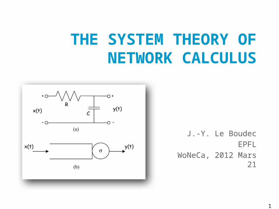
THE SYSTEM THEORY OF NETWORK CALCULUS
J.-Y. Le BoudecEPFL
WoNeCa, 2012 Mars 21
1

Contents
1. Network Calculus’s System Theory and Two Simple Examples
2. More Examples
3. Time versus Space
2

The Shaper
shaper: forces output to be constrained by greedy shaper storesdata in a buffer only if neededexamples:
constant bit rate link (s(t)=ct)ATM shaper; fluid leaky bucket controller
Pb: find input/output relation
3
sfresh traffic
R R*
shaped traffics-smooth

A Min-Plus Model of Shaper
Shaper Equations: (1)
(2) and are functions is sub-additive is min-plus convolution
4
sfresh traffic
R x
shaped traffics-smooth
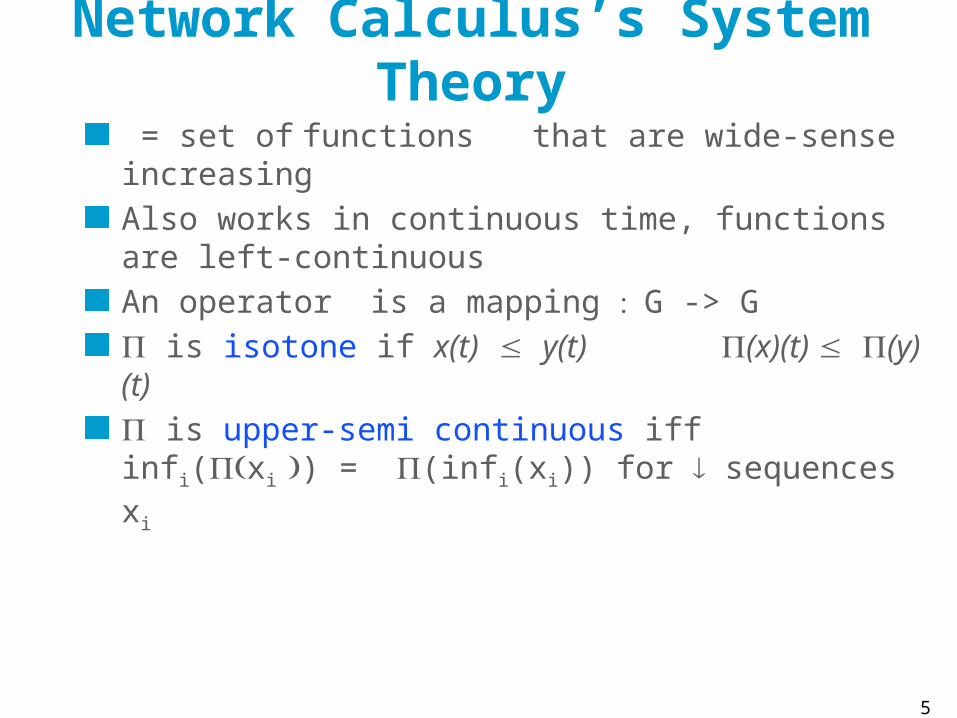
Network Calculus’s System Theory = set of functions that are wide-sense increasingAlso works in continuous time, functions are left-continuous An operator is a mapping : G -> G is isotone if x(t) y(t) (x)(t) (y)(t) is upper-semi continuous iff infi((xi )) = (infi(xi)) for sequences xi
5

Min-Plus Linear Operators is min-plus linear if
for any constant K, (x + K) = (x) + K (x y) = (x) (y)
is upper-semi continuous.
Representation Theorem: is min-plus linear <=> there is a unique H: R x R -> R+ , in and in , such that (x)(t)=infs[H(t,s)+x(s)]
min-plus linear => isotone and upper semi-continuousExample: convolution operator
Example: is given:
6

Min-Plus Residuation TheoremTheorem: ([L., Thiran 2001] thm 4.3.1., derived from Baccelli
et al., ) Assume that is isotone and upper-semi-continuous. The problem
x(t) b(t) (x)(t)where is the unknown function
has one maximum solution in , given by x*(t) = (b)(t)
(Definition of closure) (x) = inf {x, (x), (x), (x),...}
in other words: x0 = b ; xi = (xi-1) and x* = inf {x0, x1, ..., xi, ...}
7

Application to Shaper
There is a maximum solution obtained by iterating
because Thus The greedy shaper output is R*= R , the subadditive closure of is
8
(1) x x (2) x R
(1) x x (2) x R
sfresh traffic
R R*
shaped traffics-smooth

Variable Capacity Node
node has a time varying capacity µ(t)
Define M(t) =0
t m(s) ds.
the output satisfies R*(t) R(t)R*(t) -R*(s) M(t) -M(s) for all s t
and is “as large as possible”
9
fresh traffic m(t)
R R*

Variable Capacity Node
Operator : s.t.
We have the problem and the sub-additive closure of is There is a maximum solution,
10
fresh traffic m(t)
R R*
R*(t) R(t)R*(t) -R*(s) M(t) -M(s)
for all s t
MORE EXAMPLES2.
11

A System with Loss [Chuang and Cheng 2000]
node with service curve b(t) and buffer of size X when buffer is full incoming data is discarded modelled by a virtual controller (not buffered)fluid model or fixed sized packetsPb: find loss ratio
12
fresh trafficR(t)
buffer X
Loss L(t)
bR’(t) R*(t)

A System with Loss
Assume is smooth; if then no lossIf , what can we say ?
13
fresh trafficR(t)
buffer X
Loss L(t)
bR’(t) R*(t)
(t)
𝜷 (𝒕)𝑣 (𝛼 , 𝛽)
𝑡
𝑋
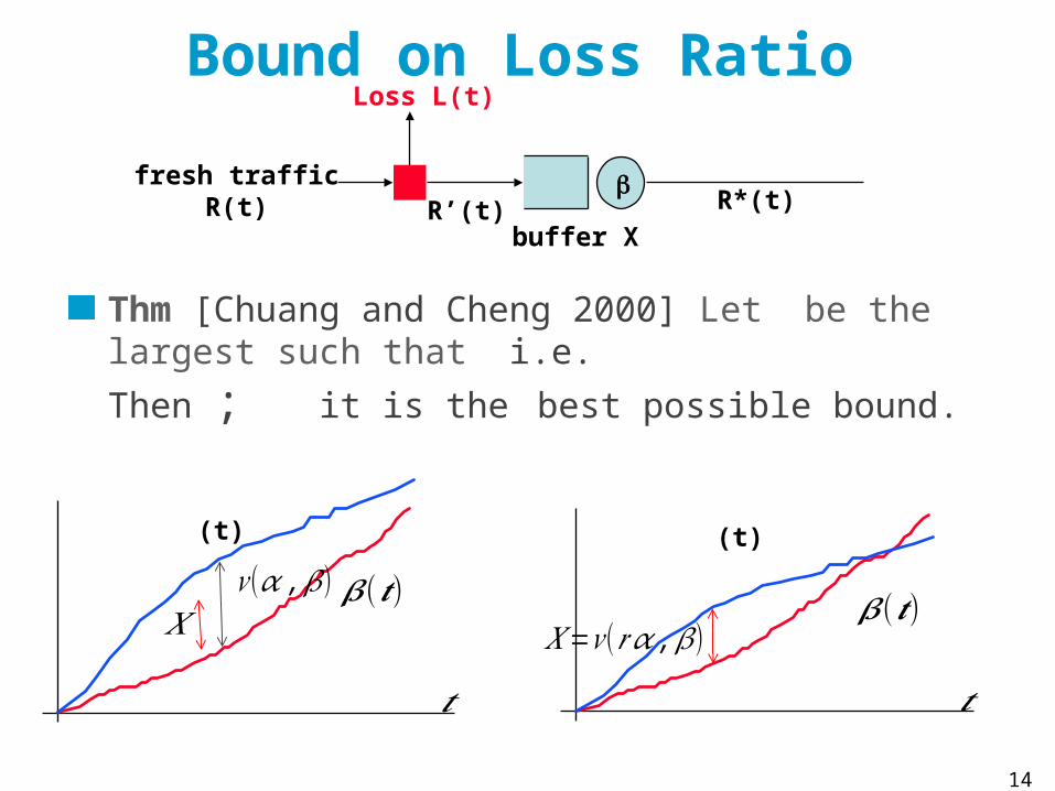
Bound on Loss Ratio
Thm [Chuang and Cheng 2000] Let be the largest such that i.e.
Then ; it is the best possible bound.
14
fresh trafficR(t)
buffer X
Loss L(t)
bR’(t) R*(t)
(t)
𝜷 (𝒕)𝑣 (𝛼 , 𝛽)
𝑡
𝑋
(t)
𝜷 (𝒕)𝑋=𝑣 (𝑟 𝛼 , 𝛽)
𝑡
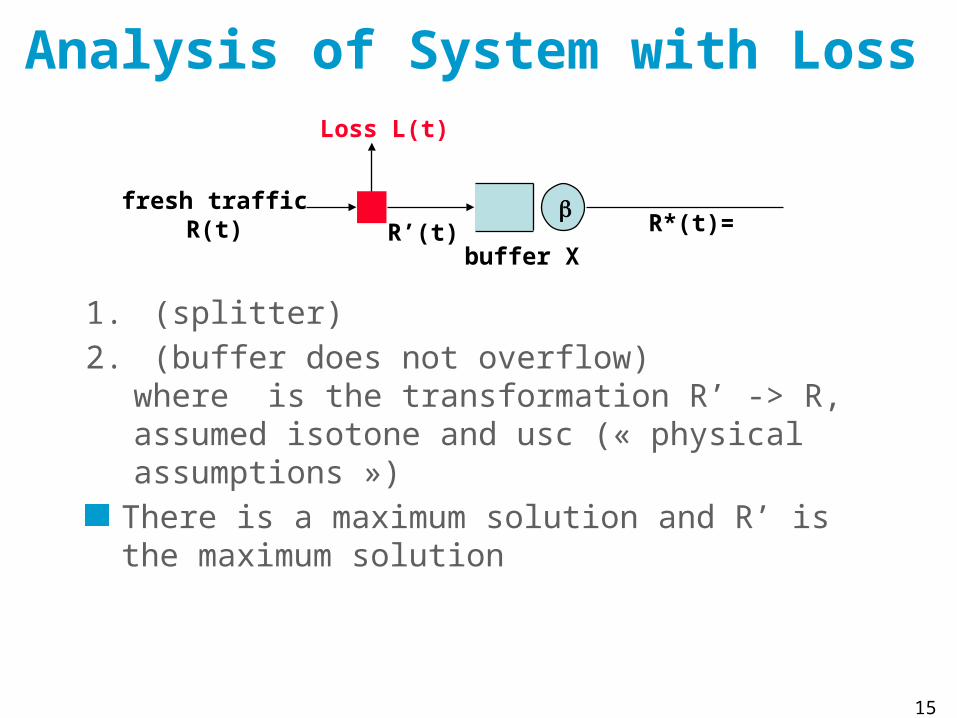
Analysis of System with Loss
1. (splitter)2. (buffer does not overflow)
where is the transformation R’ -> R, assumed isotone and usc (« physical assumptions »)
There is a maximum solution and R’ is the maximum solution
15
fresh trafficR(t)
buffer X
Loss L(t)
bR’(t) R*(t)=

Analysis of System with Loss
Let with given by thm.Eqn 1 is satisfied is smooth, thus required buffer and Eqn 2 is satisfiedThus and
16
fresh trafficR(t)
buffer X
Loss L(t)
bR’(t) R*(t)=

Optimal Smoothing [L.,Verscheure 2000]
Network + end-client offer a service curve b to flow R’(t)Smoother delivers a flow R’(t) conforming to an arrival curve s.Video stream is stored in the client buffer, read after a playback delay D.Pb: which smoothing strategy minimizes D?
17
R(t-D)R’(t) R*(t)
NetworkSmoother
ß(t)s
Video display
B
Video server
R(t)
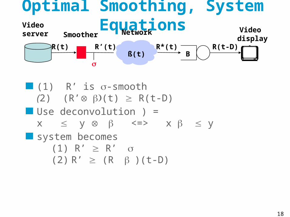
Optimal Smoothing, System Equations
(1) R’ is s-smooth(2) (R’(t) R(t-D)Use deconvolution ) = x y <=> x ysystem becomes
(1) R’ R’ s (2) R’ (R )(t-D)
18
R(t-D)R’(t) R*(t)
NetworkSmoother
ß(t)s
Video display
B
Video server
R(t)

Optimal Smoothing, System Equations
This is a max-plus linear problem, it has a minimum solution given by the iterations: (R ( ))(t-D) because
Thus
19
R(t-D)R’(t) R*(t)
NetworkSmoother
ß(t)s
Video display
B
Video server
R(t)
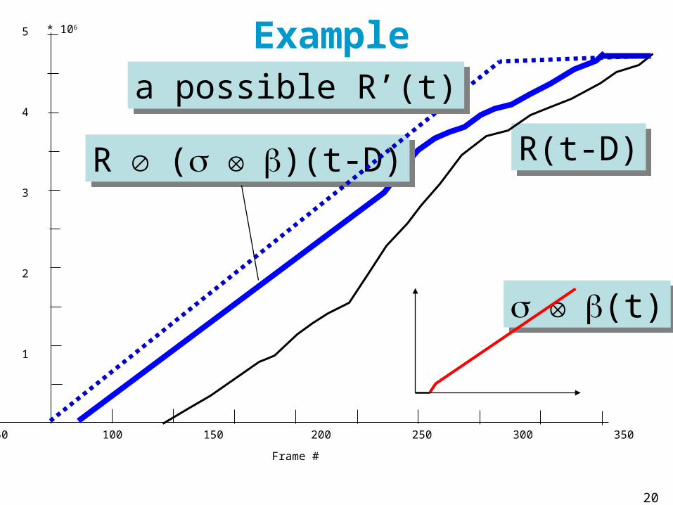
Example
20
R(t-D)R(t-D)
-50 0 50 100 150 200 250 300 350 400 450
Frame #
5
4
3
2
1
* 106
R ( s b)(t-D)R ( s b)(t-D)
s b(t) s b(t)
a possible R’(t)a possible R’(t)
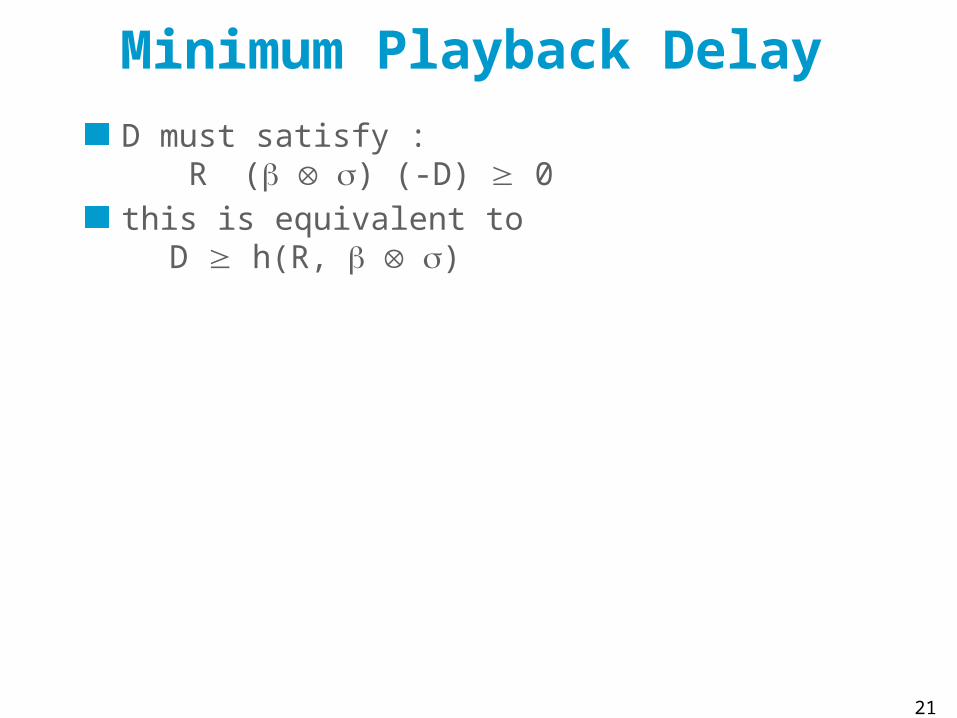
Minimum Playback DelayD must satisfy :
R ( s) (-D) 0this is equivalent to
D h(R, s)
21

22
100 200 300 400
2000
4000
6000
8000
10000 R(t)
100 200 300 40010203040506070
( )(s b t)D = 435 ms
100 200 300 400
2000
4000
6000
8000
10000
100 200 300 40010203040506070
( )(s b t)
D = 102 ms

The Perfect Battery
Battery may be charged ()or discharged ()Load is givenProblem is to determine a power schedule , subject to and within battery constraints
23

System Equations for the Perfect Battery
1. no underflow2. no overflow3. power constraint
where are cumulative functions such as
24

System Equations
25
Relax (eq 1):
There is a maximum solution,
is causalThe problem is feasible iff satisfies (eq 1), i.e.
1. no underflow2. no overflow
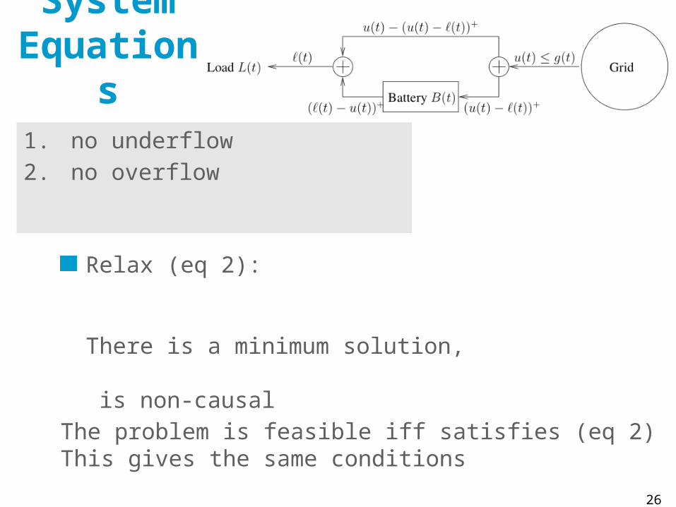
System Equations
26
Relax (eq 2):
There is a minimum solution,
is non-causalThe problem is feasible iff satisfies (eq 2)This gives the same conditions
1. no underflow2. no overflow

TIME VERSUS SPACE3.
27

The Residuation Theorem is a Space Method
The maximum solution to the problem
is given by iterates over the entire trajectory
When time is discrete there may be another way to compute by time recursion
28

The Shaper, Time Method
Time is discrete Define by:
is solution For any other solution , [induction] is the maximal solution, i.e. Note the difference in representation:
29
(1) x x (2) x R
(1) x x (2) x R
sfresh traffic
R R*
shaped traffics-smooth
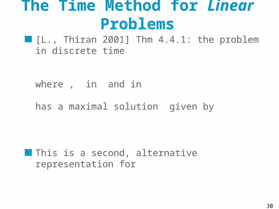
The Time Method for Linear Problems[L., Thiran 2001] Thm 4.4.1: the problem in discrete time
where , in and in
has a maximal solution given by
This is a second, alternative representation for
30

Perfect Battery
31
There is a maximum solution,
It can be computed by the time method:
The minimum schedule is anti-causal and can be computed with time reversal

ConclusionMin-plus and max-plus system theory contains a central result : residuation theorem ( = fixed point theorem)Establishes existence of maximum (resp. minimum) solutionsand provides a representation
Space and Time methods give different representations
32

Thank You…
33